One-Way ANOVA

Multiple Comparisons

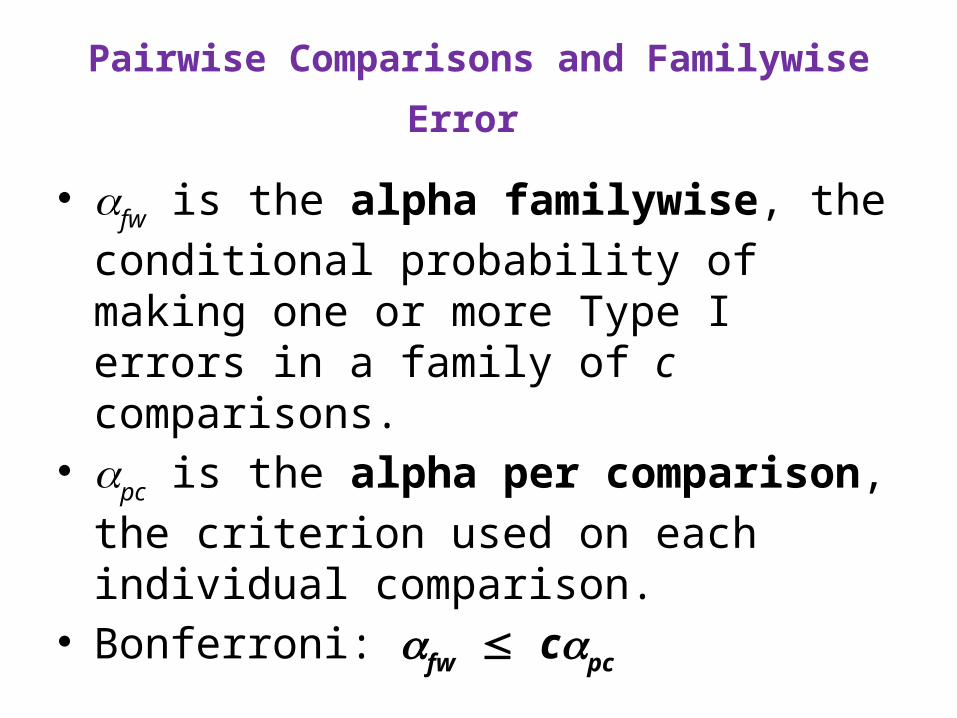
Pairwise Comparisons and Familywise Error

• fw is the alpha familywise, the conditional

probability of making one or more Type I errors in a family of c comparisons.

• pc is the alpha per comparison, the

criterion used on each individual comparison.

• Bonferroni: fw cpc

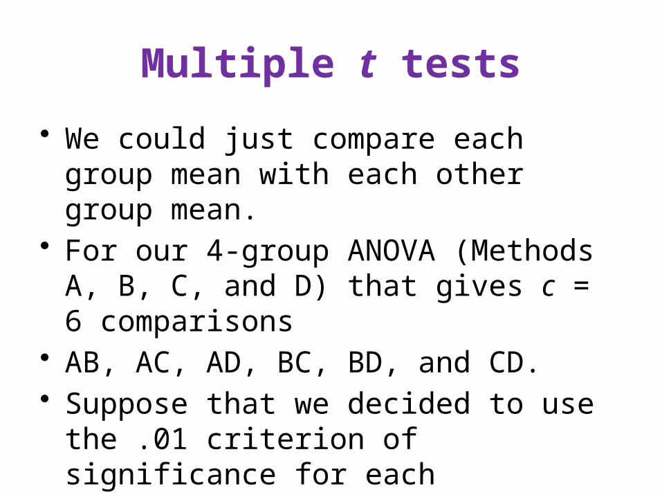
Multiple t tests

• We could just compare each group mean with each other group mean.

• For our 4-group ANOVA (Methods A, B, C, and D) that gives c = 6 comparisons

• AB, AC, AD, BC, BD, and CD.• Suppose that we decided to use the .01

criterion of significance for each comparison.

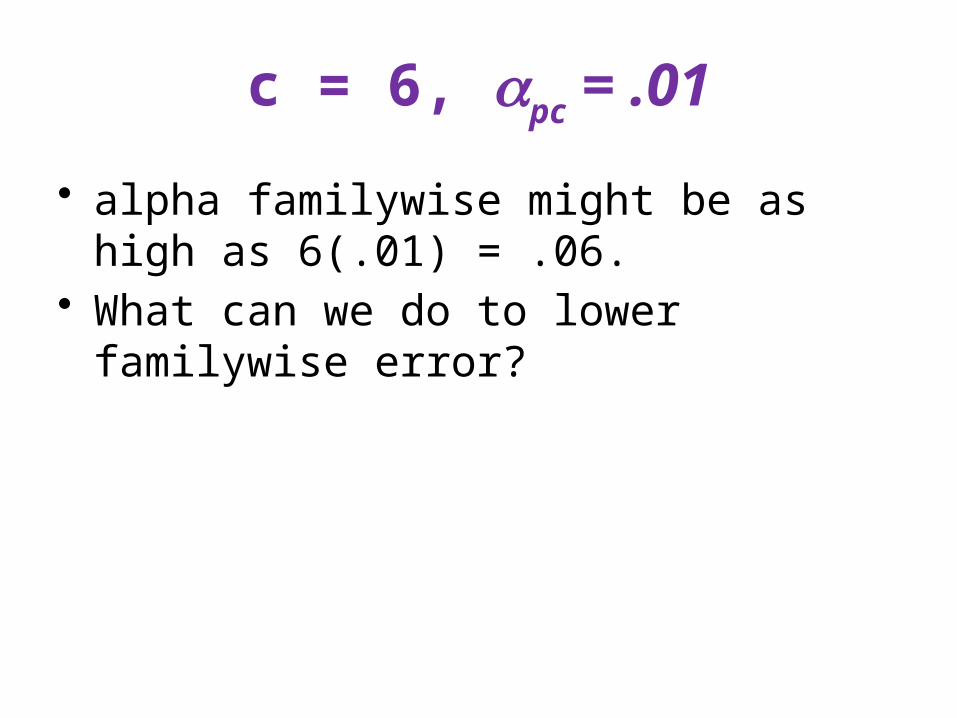
c = 6, pc = .01

• alpha familywise might be as high as 6(.01) = .06.

• What can we do to lower familywise error?

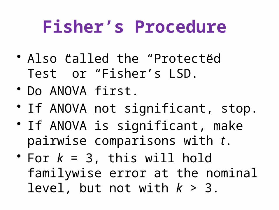
Fisher’s Procedure

• Also called the “Protected Test” or “Fisher’s LSD.”

• Do ANOVA first.• If ANOVA not significant, stop.• If ANOVA is significant, make pairwise

comparisons with t.• For k = 3, this will hold familywise error at

the nominal level, but not with k > 3.

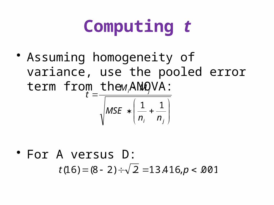
Computing t

• Assuming homogeneity of variance, use the pooled error term from the ANOVA:

• For A versus D:

ji

ji

nnMSE

MMt

11

001. ,416.132.)28()16( pt

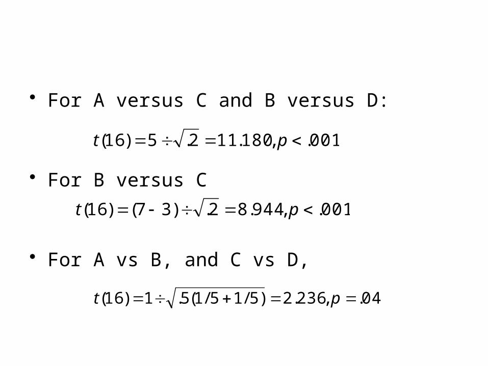
• For A versus C and B versus D:

• For B versus C

• For A vs B, and C vs D,

001. ,944.82.)37()16( pt

001. ,180.112.5)16( pt

04. ,236.2)5/15/1(5.1)16( pt

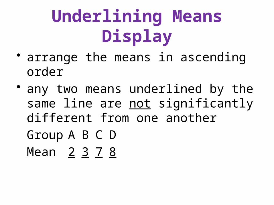
Underlining Means Display

• arrange the means in ascending order• any two means underlined by the same

line are not significantly different from one another

Group A B C D

Mean 2 3 7 8

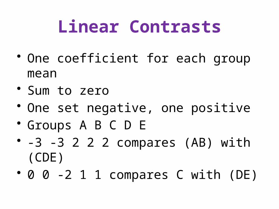
Linear Contrasts

• One coefficient for each group mean• Sum to zero• One set negative, one positive• Groups A B C D E• -3 -3 2 2 2 compares (AB) with (CDE)• 0 0 -2 1 1 compares C with (DE)

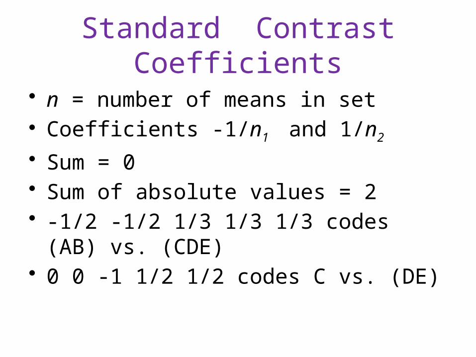
Standard Contrast Coefficients

• n = number of means in set• Coefficients -1/n1 and 1/n2

• Sum = 0• Sum of absolute values = 2• -1/2 -1/2 1/3 1/3 1/3 codes (AB) vs. (CDE)• 0 0 -1 1/2 1/2 codes C vs. (DE)

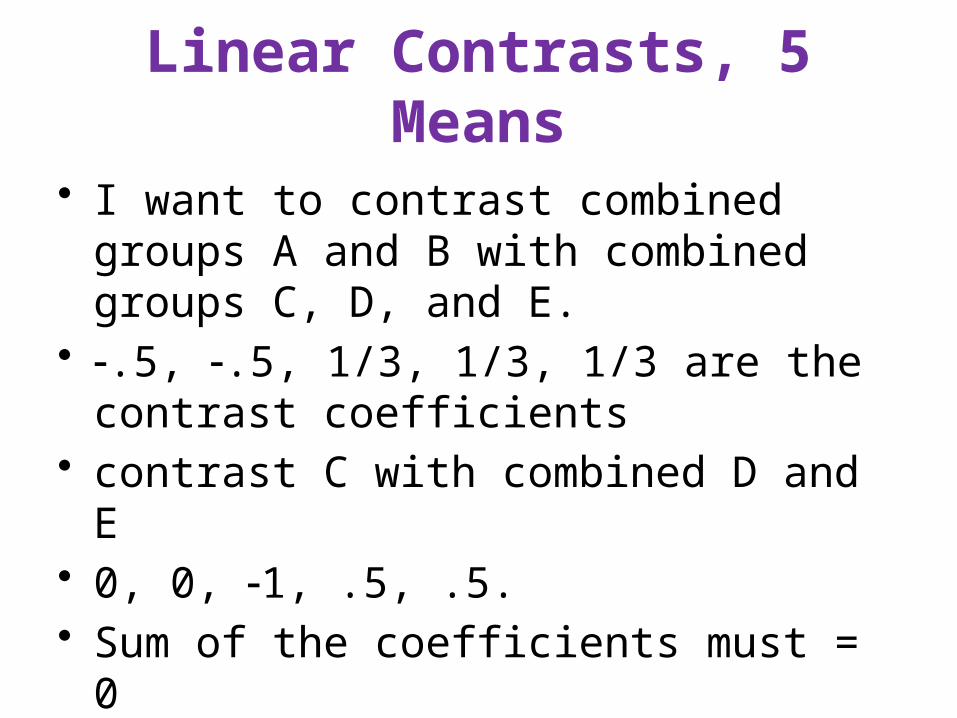
Linear Contrasts, 5 Means

• I want to contrast combined groups A and B with combined groups C, D, and E.

• .5, .5, 1/3, 1/3, 1/3 are the contrast coefficients

• contrast C with combined D and E• 0, 0, 1, .5, .5.• Sum of the coefficients must = 0• One set is positive, the other negative

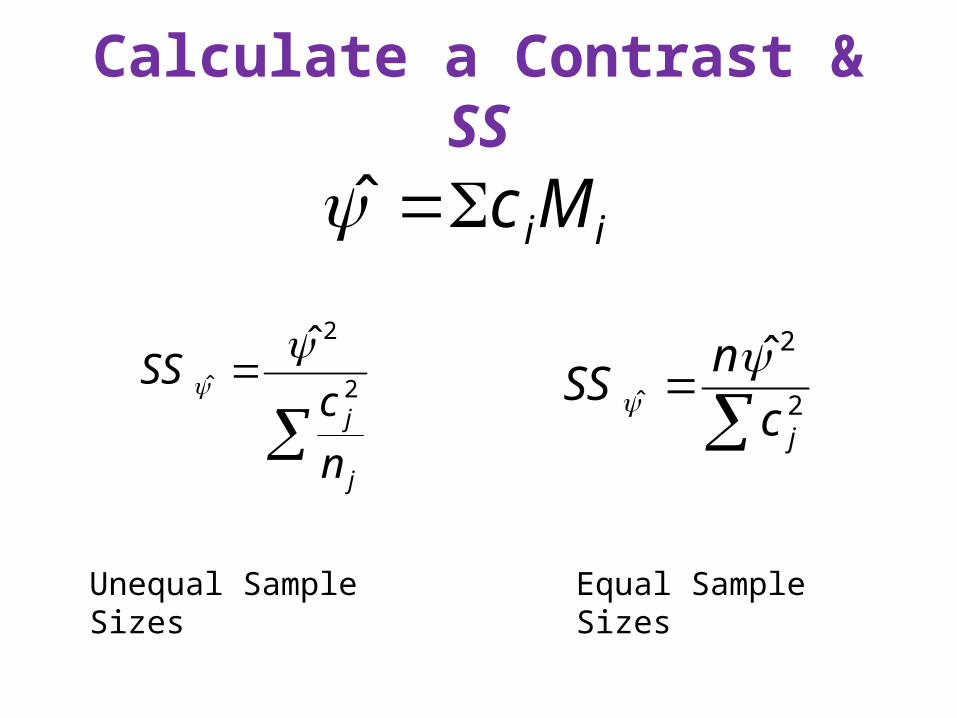
Calculate a Contrast & SS

iiMc

j

j

n

cSS

2

2

ˆ

2

2

ˆ

ˆ

jcn

SS

Unequal Sample Sizes Equal Sample Sizes

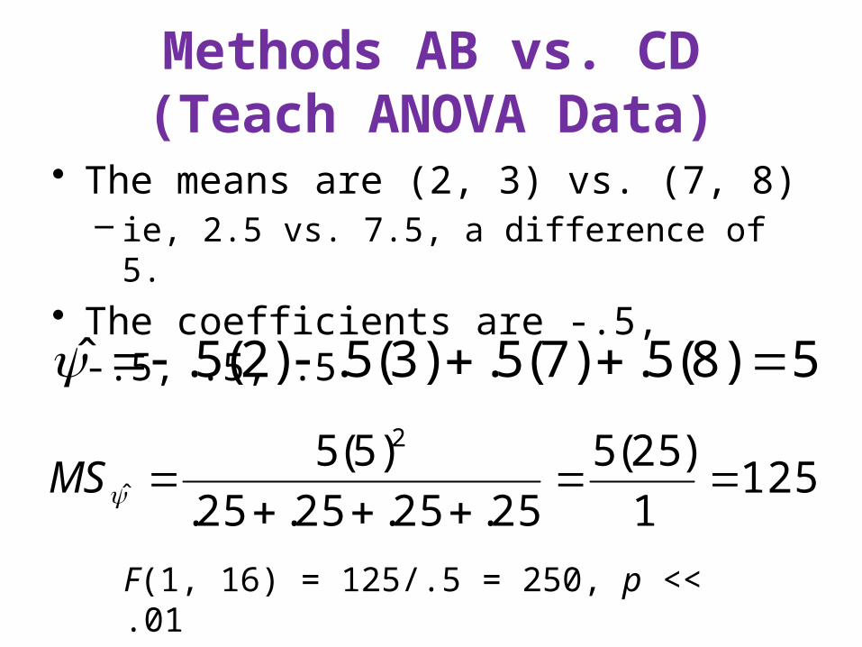
Methods AB vs. CD (Teach ANOVA Data)

• The means are (2, 3) vs. (7, 8)– ie, 2.5 vs. 7.5, a difference of 5.

• The coefficients are -.5, -.5, .5, .5

5)8(5.)7(5.)3(5.)2(5.ˆ

1251

)25(525.25.25.25.

)5(5 2

ˆ

MS

F(1, 16) = 125/.5 = 250, p << .01

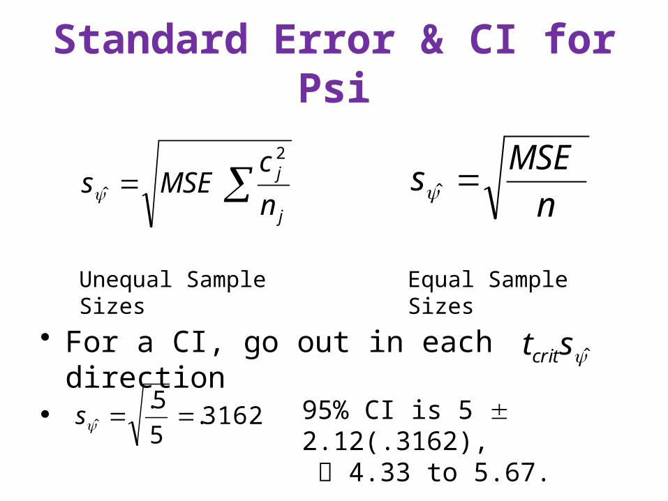
Standard Error & CI for Psi

• For a CI, go out in each direction•

j

j

n

cMSEs

2

nMSE

s

Unequal Sample Sizes Equal Sample Sizes

stcrit

3162.5

5.ˆ s 95% CI is 5 2.12(.3162),

4.33 to 5.67.

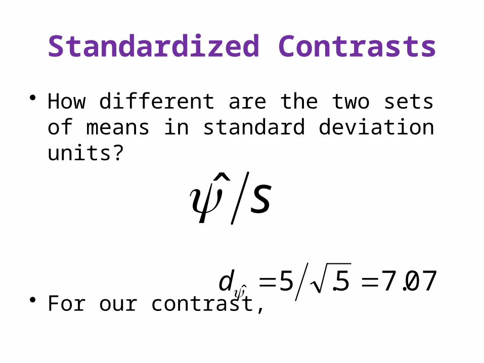
Standardized Contrasts

• How different are the two sets of means in standard deviation units?

• For our contrast,

s07.75.5ˆ d

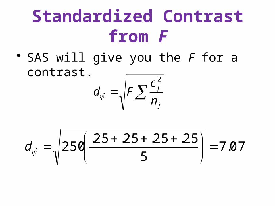
Standardized Contrast from F

• SAS will give you the F for a contrast.

j

j

n

cFd

2

07.75

25.25.25.25.250ˆ

d

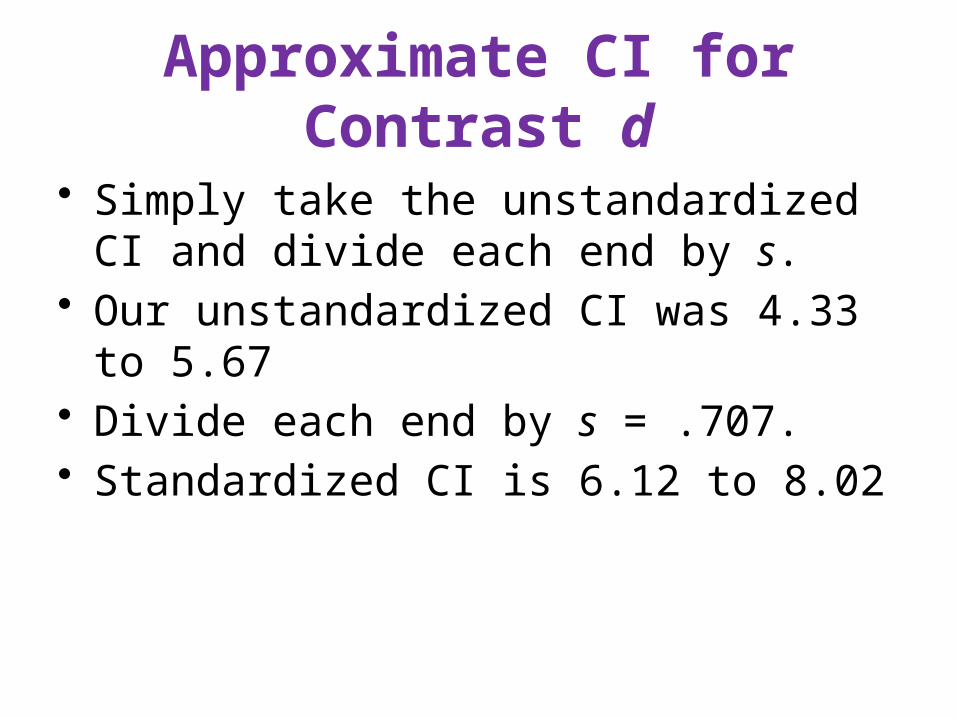
Approximate CI for Contrast d

• Simply take the unstandardized CI and divide each end by s.

• Our unstandardized CI was 4.33 to 5.67• Divide each end by s = .707.• Standardized CI is 6.12 to 8.02

Exact CI for Contrast d

• Conf_Interval-Contrast.sas • The CI extends from 4.48 to 9.64 • Notice that this is considerably wider than

the approximate CI

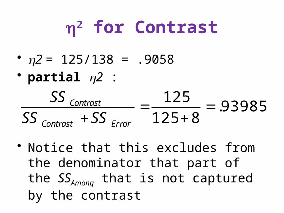
2 for Contrast

• 2 = 125/138 = .9058 • partial 2 :

• Notice that this excludes from the denominator that part of the SSAmong that is not captured by the contrast

93985.8125

125

ErrorContrast

Contrast

SSSSSS

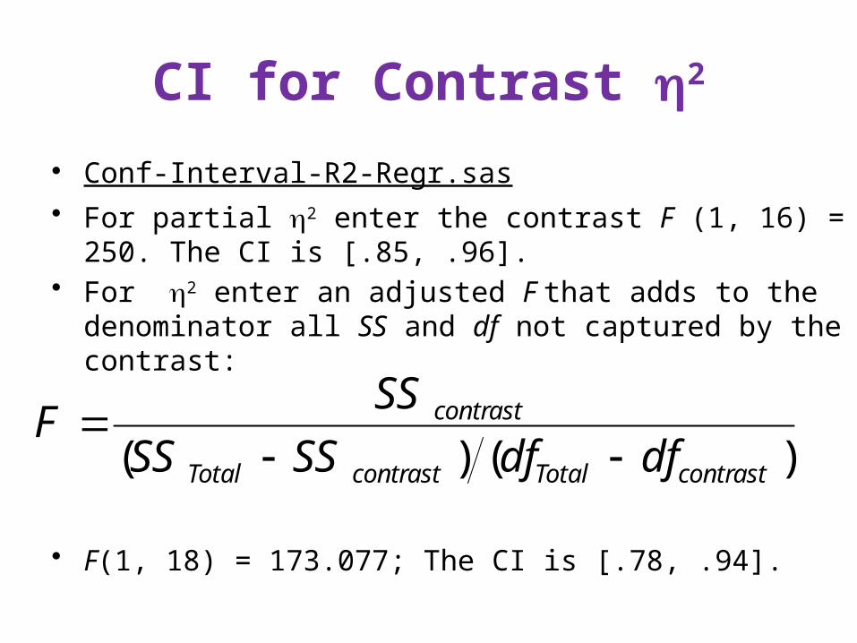
CI for Contrast 2

• Conf-Interval-R2-Regr.sas • For partial 2 enter the contrast F (1, 16) = 250. The CI is

[.85, .96].• For 2 enter an adjusted F that adds to the denominator all

SS and df not captured by the contrast:

• F(1, 18) = 173.077; The CI is [.78, .94].

)()( contrastTotalcontrastTotal

contrast

dfdfSSSS

SSF

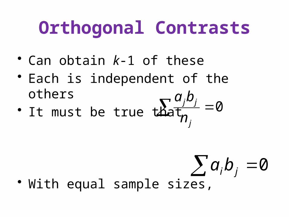
Orthogonal Contrasts

• Can obtain k-1 of these• Each is independent of the others• It must be true that

• With equal sample sizes,

0j

jj

n

ba

0 ji ba

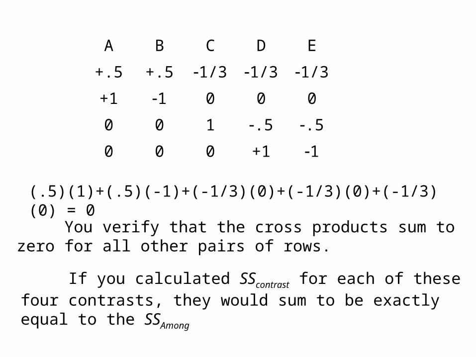
A B C D E

+.5 +.5 1/3 1/3 1/3

+1 1 0 0 0

0 0 1 .5 .50 0 0 +1 1

(.5)(1)+(.5)(-1)+(-1/3)(0)+(-1/3)(0)+(-1/3)(0) = 0

You verify that the cross products sum to zero for all other pairs of rows.

If you calculated SScontrast for each of these four contrasts, they would sum to be exactly equal to the SSAmong

Procedures Designed to Cap FW

• We have already discussed Fisher’s Procedure, which does require that the ANOVA be significant.

• None of the other procedures require that the ANOVA be significant.

• They were designed to replace the ANOVA, not be done after an ANOVA.

A Common Delusion

• Many mistakenly believe that all procedures require a significant ANOVA.

• This is like being so paranoid about getting an STD that you abstain from sex and wear a condom.

• If you have done the one, you do not also need to do the other.

Studentized Range Procedures

• These are often used when one wishes to compare each group mean with each other group mean.

• I prefer to make only comparisons that address a research question.

• The test statistic is q.• See the handout for an example using the

Student Newman Keuls procedure.

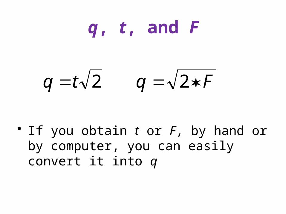
q, t, and F

• If you obtain t or F, by hand or by computer, you can easily convert it into q

2tq Fq 2

Tukey’s (a) Honestly Significant Difference Test

• If part of the null is true and part false, the SNK can allow to exceed its nominal level.

• Tukey’s HSD is more conservative, and does not allow to exceed its nominal level.

Tukey’s (b) Wholly Significant Difference Test

• SNK too liberal, HSD too conservative, OK let us compromise.

• For the WSD the critical value of q is the simple mean of what it would be for the SNK and what it would be for the HSD.

Ryan-Einot-Gabriel-Welsch Test

• Holds familywise error at the stated level.• Has more power than other techniques

which also adequately control familywise error.

• SAS and SPSS will do it for you.• It is much too difficult to do by hand.

Which Test Should I Use?

• If k = 3, use Fisher’s Procedure• If k > 3, use REGWQ• Remember, ANOVA does not have to be

significant to use REGWQ or any of the procedures covered here other than Fisher’s procedure.

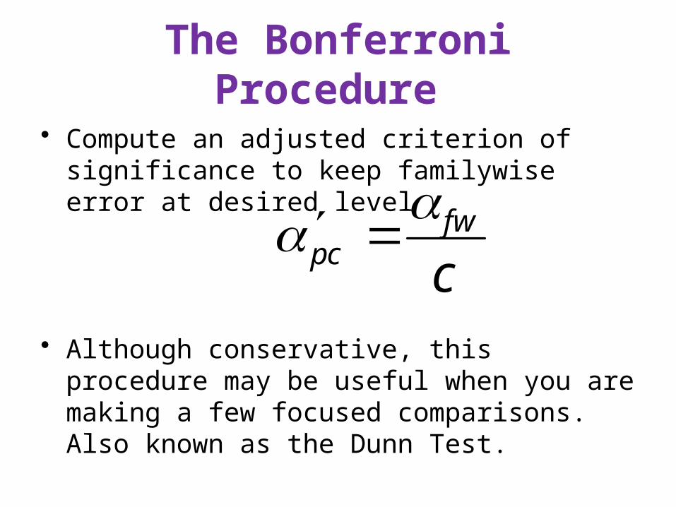
The Bonferroni Procedure

• Compute an adjusted criterion of significance to keep familywise error at desired level

• Although conservative, this procedure may be useful when you are making a few focused comparisons. Also known as the Dunn Test.

cfw

pc

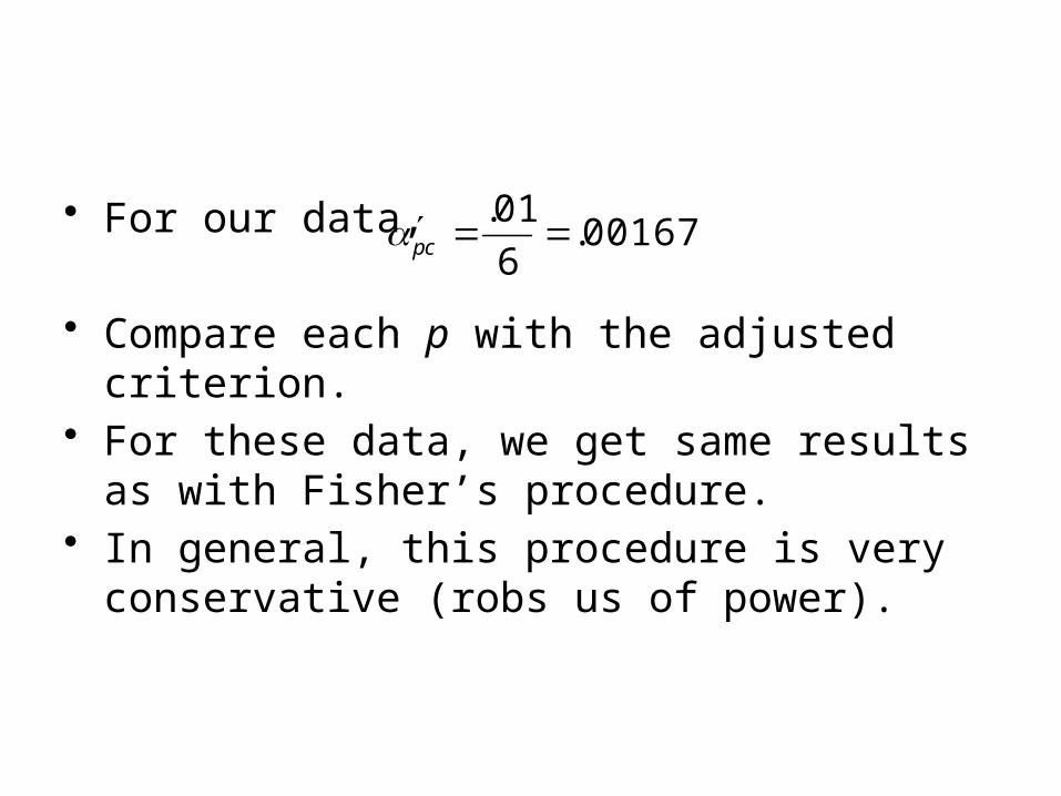
• For our data,

• Compare each p with the adjusted criterion.• For these data, we get same results as with

Fisher’s procedure.• In general, this procedure is very conservative

(robs us of power).

00167.6

01. pc

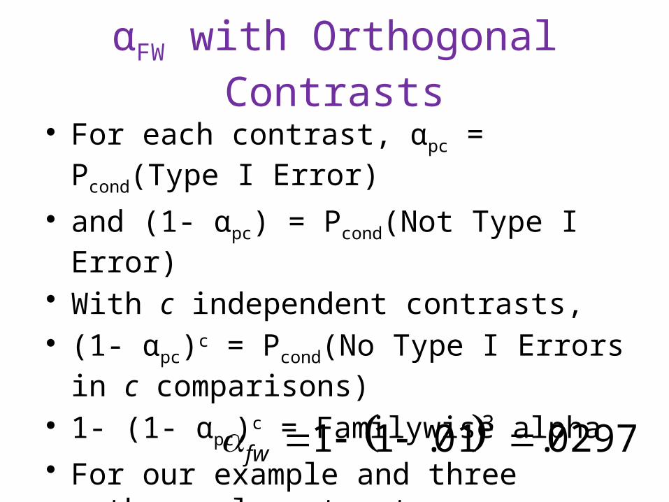
αFW with Orthogonal Contrasts

• For each contrast, αpc = Pcond(Type I Error)

• and (1- αpc) = Pcond(Not Type I Error)

• With c independent contrasts,• (1- αpc)c = Pcond(No Type I Errors in c

comparisons)• 1- (1- αpc)c = Familywise alpha

• For our example and three orthogonal contrasts, 0297.01.11 3 fw

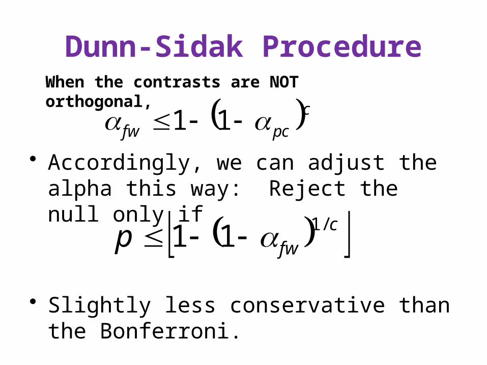
Dunn-Sidak Procedure

• Accordingly, we can adjust the alpha this way: Reject the null only if

• Slightly less conservative than the Bonferroni.

cpcfw 11

cfwp /111

When the contrasts are NOT orthogonal,

Scheffé Test

• Assumes you make every possible contrast, not just each mean with each other.

• Very conservative.• adjusted critical F equals (the critical value

for the treatment effect from the omnibus ANOVA) times (the treatment degrees of freedom from the omnibus ANOVA).

Dunnett’s Test

• Used only when you are comparing each treatment group with a single control group.

• Compute t as with the Bonferroni or LSD test.

• Then use a special table of critical values.

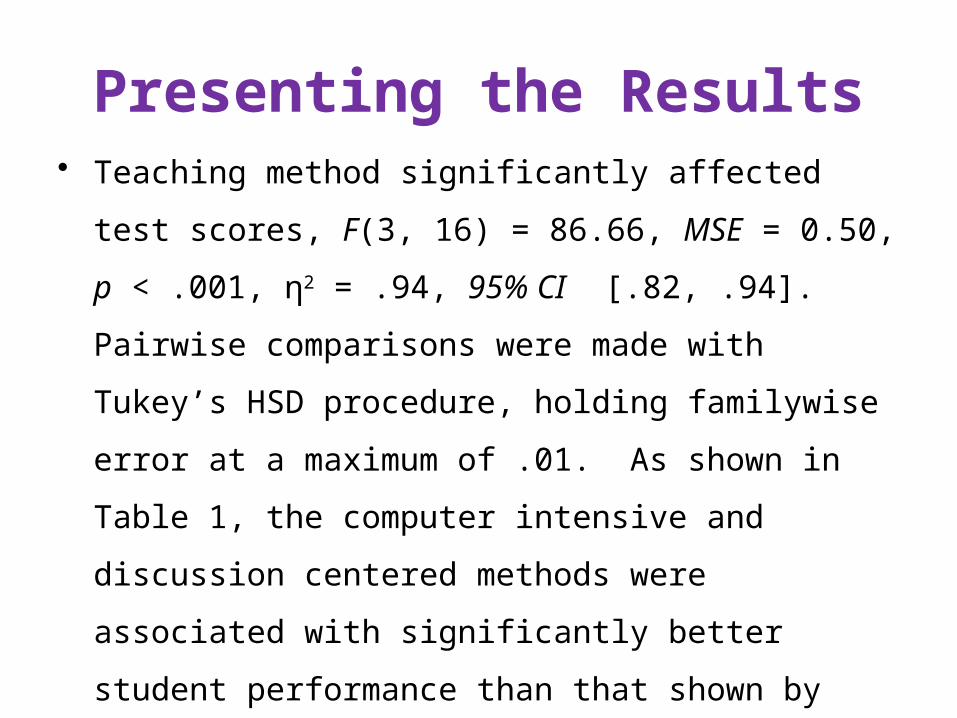
Presenting the Results• Teaching method significantly affected test scores, F(3,

16) = 86.66, MSE = 0.50, p < .001, η2 = .94, 95% CI

[.82, .94]. Pairwise comparisons were made with

Tukey’s HSD procedure, holding familywise error at a

maximum of .01. As shown in Table 1, the computer

intensive and discussion centered methods were

associated with significantly better student performance

than that shown by students taught with the actuarial and

book only methods. All other comparisons fell short of

statistical significance.

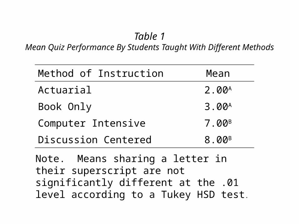
Method of Instruction Mean

Actuarial 2.00A

Book Only 3.00A

Computer Intensive 7.00B

Discussion Centered 8.00B

Note. Means sharing a letter in their superscript are not significantly different at the .01 level according to a Tukey HSD test.

Table 1Mean Quiz Performance By Students Taught With Different Methods

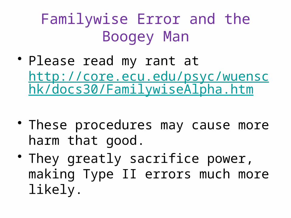
Familywise Error and the Boogey Man

• Please read my rant at http://core.ecu.edu/psyc/wuenschk/docs30/FamilywiseAlpha.htm

• These procedures may cause more harm that good.

• They greatly sacrifice power, making Type II errors much more likely.