Online Appendix for “How Do Electricity Shortages A … Appendix for “How Do Electricity Shortages A↵ect Industry? Evidence from India ... Anuradha Bhatta,

Online Appendix for “How Do Electricity Shortages A↵ectIndustry? Evidence from India”

By Hunt Allcott, Allan Collard-Wexler, and Stephen D.O’Connell

.

2005 World Bank Enterprise Survey: Barriers to Growth

⇤ Allcott: New York University, NBER, and Poverty Action Lab. NYU Economics Department, 19W. 4th St., New York, NY 10012. Email: [email protected]. Collard-Wexler: Duke University andNBER. 230 Social Sciences Building, Durham, NC 27708. Email: [email protected]. O’Connell:City University of New York - Graduate Center. Department of Economics Room 5313, 365 5th Av-enue, New York, NY 10016. Email: [email protected]. We thank Maureen Cropper, JanDe Loecker, Michael Greenstone, Peter Klenow, Kabir Malik, Rohini Pande, Nick Ryan, JagadeeshSivadasan, Anant Sudarshan, and seminar participants at Brown, Drexel, Duke, the Federal Trade Com-mission, Harvard, the 2013 NBER Summer Institute, the 2014 NBER Winter IO/EEE meetings, Soci-ety for Economic Dynamics, Stanford, KU Leuven, Toulouse, Universidad de los Andes, University ofChicago, University of Cologne, and the World Bank for helpful comments. We are particularly gratefulto Nick Bloom, Troy Smith, and Shaleen Chavda for insight into the textile industry. We thank DeepakChoudhary, Anuradha Bhatta, Sherry Wu, and Mark Thomas for helpful research assistance and theStern Center for Global Economy and Business for financial support. We have benefited from helpfulconversations with Jayant Deo of India Energy Exchange, Gajendra Haldea of the Planning Commission,Partha Mukhopadhyay of the Centre for Policy Research, and Kirit Parikh of IGIDR. We also thank A.S. Bakshi and Hemant Jain of the Central Electricity Authority for help in collecting archival data. Ofcourse, all analyses are the responsibility of the authors, and no other parties are accountable for ourconclusions. The authors declare that they have no relevant or material financial interests that relate tothe research described in this paper.

1

2 THE AMERICAN ECONOMIC REVIEW

Table A1—: Biggest Obstacle for Growth

Problem PercentElectricity 33High Taxes 16Corruption 10Tax Administration 8Cost of and Access to Financing 6Labor Regulations and Business Licensing 5Skills and Education of Available Workers 4Access to Land 3Customs and Trade Regulations 2Other 12

Notes: These data are from the 2005 World Bank Enterprise Survey in India. The table presentsresponses to the question, “Which of the elements of the business environment included in the list, ifany, currently represents the biggest obstacle faced by this establishment?”

VOL. NO. ONLINE APPENDIX FOR “HOW DO ELECTRICITY SHORTAGES AFFECT INDUSTRY?”3

Power Sector Data Appendix

This appendix provides additional details on the power sector data in SectionI.I.B.Appendix Table A1 presents the state allocations from jointly-owned power

plants.Appendix Table A2 presents summary statistics for the reservoir and hydro

plant microdata. Panel A presents the reservoir microdata; 31 reservoirs everappear. A reservoir scheme may include multiple hydro plants, so generation andgeneration capacity are for all plants within the reservoir scheme. All reservoirdata are missing for the year 2000, so inflows are imputed using rainfall at grid-points within the reservoir watershed. For each reservoir, we then run a regressionof generation on inflows; the fitted values are then divided by generation capacityand transformed into a predicted capacity factor.Panel B of Appendix Table A2 presents the hydro plant microdata; 181 plants

ever appear, of which 18 percent (32 plants) are known to be run-of-river plants.All plant-level data are missing for the year 1992, and generation data are occa-sionally missing in other years. Just less than six percent of generation observa-tions are imputed using rainfall at gridpoints within the plant’s watershed.Appendix Table A3 presents summary statistics on electricity supply for the

ten largest states.Figures A1, A2, A3 present maps of shortage severity, hydro power plants and

weather stations, and four example hydro plant watersheds, respectively.


Table A1—: State Allocations from Jointly-Owned Hydro Plants

Share TotalPower Station State (Percent) Capacity (MW)Bhakra Nangal Complex Haryana 33.91 1479.5

Punjab 50.87Rajasthan 15.22

Dehar Haryana 32 990Punjab 48Rajasthan 20

Pong Haryana 16.6 396Punjab 24.9Rajasthan 58.5

Gandhi Sagar Madhya Pradesh 50 115Rajasthan 50

Jawahar Sagar Madhya Pradesh 50 99Rajasthan 50

Rana Pratap Sagar Madhya Pradesh 50 172Rajasthan 50

Machkund Andhra Pradesh 70 114.75Orissa 30

Tungabhadra/Hampi Andhra Pradesh 80 72Karnataka 20

Pench Madhya Pradesh 66.67 160Maharashtra 33.33

Sardar Sarovar Gujarat 16 1450Madhya Pradesh 57Maharashtra 27

Rajghat Madhya Pradesh 50 45Uttar Pradesh 50

Ranjit Sagar Punjab 75.4 600Jammu & Kashmir 20Himachal Pradesh 4.6

Source: Central Electricity Authority, General Review 2012.


Table A2—: Reservoir and Hydro Plant Microdata Summary Statistics

Panel A: Reservoir MicrodataMean Std. Dev. Min. Max. Obs.

Reservoir Years Observed 12.4 7.0 4 19 31Reservoir Inflows (billion cubic meters) 9.0 11.1 0.14 77.4 362Reservoir-Level Generation (GWh) 1926 1669 27 8016 367Reservoir-Level Generation Capacity (MW) 676 547 75 1956 383Capacity Factor Predicted by Inflows 0.36 0.14 0.09 0.75 383

Panel B: Hydro Plant Generation MicrodataMean Std. Dev. Min. Max. Obs.

Plant Years Observed 14.0 6.1 1 19 181Run-of-River Plant 0.19 0.4 0.00 1.0 177Generation (GWh) 654 1042 0 13211 2395Capacity (MW) 207 304 0 1956 2505Capacity Factor 0.37 0.19 0 1.57 2387

Notes: Reservoir Years Observed is at the reservoir level; all other variables in Panel A are at thereservoir-by-year level. Plant Years Observed and run-of-river categorization are at the plant level; allother variables in Panel B are at the plant-by-year level.

Table A3—: Electricity Statistics for the Ten Largest States

1992-2010 Shortages 2010 1992-2010Capacity Generation

State Mean Min. Max. (gigawatts) Share HydroAndhra Pradesh 0.08 0.01 0.22 10.8 0.21Gujarat 0.08 0.03 0.16 11.4 0.03Karnataka 0.12 0.01 0.27 9.1 0.47Madhya Pradesh 0.12 0.05 0.20 4.9 0.14Maharashtra 0.10 0.02 0.21 16.1 0.11Punjab 0.05 0.01 0.14 5.1 0.40Rajasthan 0.03 0.00 0.07 5.7 0.18Tamil Nadu 0.06 0.00 0.14 11.6 0.13Uttar Pradesh 0.15 0.10 0.22 5.5 0.11West Bengal 0.02 0.00 0.06 7.4 0.03

Notes: Shortage data are estimated by the Central Electricity Authority. 2010 Generation Capacity isreported in the CEA General Review 2012, and Generation Share Hydro is is the ratio of hydroelectricityto total generation, both of which are reported in the General Review.


Figure A1. : Map of Average Shortages by State

Notes: This figure presents each state’s average Shortage assessed by the Central Electricity Authorityover 1992-2010, with darker color illustrating higher Shortage.


Figure A2. : Hydro Power Plants, Rainfall Gridpoints, and WeatherStations

! !

! ! !

! ! ! ! !

! ! ! ! !

! ! ! ! ! ! !

! ! ! ! ! ! ! !

! ! ! ! ! ! ! !

! ! ! ! ! ! ! ! ! !

! ! ! ! ! ! ! ! ! ! !

! ! ! ! ! ! ! ! ! ! !

! ! ! ! ! ! ! ! ! ! ! !

! ! ! ! ! ! ! ! ! ! !

! ! ! ! ! ! ! ! ! ! !

! ! ! ! ! ! ! ! ! ! ! !

! ! ! ! ! ! ! ! ! ! ! !

! ! ! ! ! ! ! ! ! ! ! ! ! !

! ! ! ! ! ! ! ! ! ! ! ! ! ! !

! ! ! ! ! ! ! ! ! ! ! ! ! ! ! ! ! !

! ! ! ! ! ! ! ! ! ! ! ! ! ! ! ! ! ! !

! ! ! ! ! ! ! ! ! ! ! ! ! ! ! ! ! ! ! ! !

! ! ! ! ! ! ! ! ! ! ! ! ! ! ! ! ! ! ! ! ! !

! ! ! ! ! ! ! ! ! ! ! ! ! ! ! ! ! ! ! ! ! ! !

! ! ! ! ! ! ! ! ! ! ! ! ! ! ! ! ! ! ! ! ! ! ! !

! ! ! ! ! ! ! ! ! ! ! ! ! ! ! ! ! ! ! ! ! ! ! ! ! !

! ! ! ! ! ! ! ! ! ! ! ! ! ! ! ! ! ! ! ! ! ! ! ! ! ! ! !

! ! ! ! ! ! ! ! ! ! ! ! ! ! ! ! ! ! ! ! ! ! ! ! ! ! ! ! !

! ! ! ! ! ! ! ! ! ! ! ! ! ! ! ! ! ! ! ! ! ! ! ! ! ! ! ! ! ! ! ! !

! ! ! ! ! ! ! ! ! ! ! ! ! ! ! ! ! ! ! ! ! ! ! ! ! ! ! ! ! ! ! ! ! ! ! ! ! !

! ! ! ! ! ! ! ! ! ! ! ! ! ! ! ! ! ! ! ! ! ! ! ! ! ! ! ! ! ! ! ! ! ! ! ! ! ! ! ! !

! ! ! ! ! ! ! ! ! ! ! ! ! ! ! ! ! ! ! ! ! ! ! ! ! ! ! ! ! ! ! ! ! ! ! ! ! !

! ! ! ! ! ! ! ! ! ! ! ! ! ! ! ! ! ! ! ! ! ! ! ! ! ! ! ! ! ! ! ! ! ! ! ! ! ! ! ! ! ! !

! ! ! ! ! ! ! ! ! ! ! ! ! ! ! ! ! ! ! ! ! ! ! ! ! ! ! ! ! ! ! ! ! ! ! ! ! ! ! ! ! ! ! ! ! !

! ! ! ! ! ! ! ! ! ! ! ! ! ! ! ! ! ! ! ! ! ! ! ! ! ! ! ! ! ! ! ! ! ! ! ! ! ! ! ! ! !

! ! ! ! ! ! ! ! ! ! ! ! ! ! ! ! ! ! ! ! ! ! ! ! ! ! ! ! ! ! ! ! ! ! ! ! ! !

! ! ! ! ! ! ! ! ! ! ! ! ! ! ! ! ! ! ! ! ! ! ! ! ! ! ! ! ! ! ! ! ! ! ! ! ! ! ! ! ! ! ! ! !

! ! ! ! ! ! ! ! ! ! ! ! ! ! ! ! ! ! ! ! ! ! ! ! ! ! ! ! ! ! ! ! ! ! ! ! ! ! ! ! ! ! ! ! ! !

! ! ! ! ! ! ! ! ! ! ! ! ! ! ! ! ! ! ! ! ! ! ! ! ! ! ! ! ! ! ! ! ! ! ! ! ! ! ! ! ! ! ! ! ! ! ! ! !

! ! ! ! ! ! ! ! ! ! ! ! ! ! ! ! ! ! ! ! ! ! ! ! ! ! ! ! ! ! ! ! ! ! ! ! ! ! ! ! ! ! ! ! ! !

! ! ! ! ! ! ! ! ! ! ! ! ! ! ! ! ! ! ! ! ! ! ! ! ! ! ! ! ! ! ! ! ! ! ! ! ! ! ! !

! ! ! ! ! ! ! ! ! ! ! ! ! ! ! ! ! ! ! ! ! ! ! ! ! ! ! ! ! ! ! ! ! ! ! ! !

! ! ! ! ! ! ! ! ! ! ! ! ! ! ! ! ! ! ! ! ! ! ! ! ! ! ! !

! ! ! ! ! ! ! ! ! ! ! ! ! ! ! ! ! ! ! ! !

! ! ! ! ! ! ! ! ! ! ! ! ! ! ! ! !

! ! ! ! ! ! ! ! ! ! ! ! ! !

! ! ! ! ! ! ! ! ! ! ! ! ! !

! ! ! ! ! ! ! ! ! ! !

! ! ! ! ! ! ! ! !

! ! ! ! ! ! ! !

! ! ! ! ! !

! ! ! ! ! ! ! ! ! !

! ! ! ! ! ! ! ! ! !

! ! ! ! ! ! ! ! ! !

! ! ! ! ! ! ! ! ! !

! ! ! !

!

!

!!

!

!

!

!

!

!

!

!

!

!!

!

!!!

!

!

!

!

!

!

!

!

!

!

!!

!!

!

!!

!

!

!

!

!!!

!!

!

!

!!!

! !

!!

!

!

!

!

!

!

!

!

!!!

!

!

!

!

!

!

!

!

!

!

!!

!! !

!

!

!!!!

!

!

!!!

!!!

!

!

!

!!

!

!

!!

!

!

!

!

!

!

!

!!

!

!

!

!

!

!

!

!

!

!

!

!

!

!

!!! !

!

!!

!

!

!!

!!!

!

!

!

!

!!!

!

!

!

!

!

!

!!!

!

!

!

!!

!

!

!

!

!

!

!

!

!

!

!

!!

!

!

!!!!

!!

!

! !

!

!!

!

# ####

####

# #### #####

# #### ###

## ##

## ####

#### ## ##

## ##### # ### #

######

##### #### ##

### ### ## # #

## # ## # # ### ### #

# # # ## ### # ## ## # ##

###### ## # ## # ## #

###

####

##

# ##

##

#

Legend# GSOD and GHCN weather stations, 1992-2010! Hydroelectric power plants! Univ. Delaware 1/2-degree rainfall gridpoints

Notes: This figure plots the 1/2 degree gridpoints in the University of Delaware rainfall data, theweather stations whose measurements underlie the gridded data, and the locations of all hydroelectricpower stations in India.


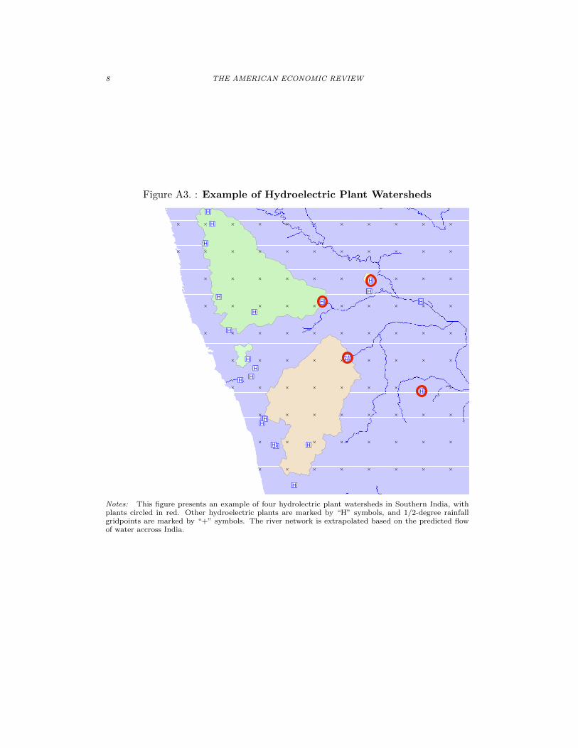
Figure A3. : Example of Hydroelectric Plant Watersheds

D D D

D D D D D D

D D D D D

D D D D D D D

D D D D D D

D D D D D D D

D D D D D D D D D

D D D D D D D D D

D D D D D D D D D D

D D D D D D D D D D D

D D D D D D D D D D D

D D D D D D D D D D D D



D D D D D D D D D D D D D

D D D D D D D D D D D D D D

D D D D D D D D D D D D D D D D

D D D D D D D D D D D D D D D D D D D D D

D D D D D D D D D D D D D D D D D D D D D D D D D D

D D D D D D D D D D D D D D D D D D D D D D D D D D D

D D D D D D D D D D D D D D D D D D D D D D D D D D D D D

D D D D D D D D D D D D D D D D D D D D D D D D D D D D D D

D D D D D D D D D D D D D D D D D D D D D D D D D D D D D D D D

D D D D D D D D D D D D D D D D D D D D D D D D D D D D D D D D D

D D D D D D D D D D D D D D D D D D D D D D D D D D D D D D D D D D D D

D D D D D D D D D D D D D D D D D D D D D D D D D D D D D D D D D D D D D D

D D D D D D D D D D D D D D D D D D D D D D D D D D D D D D D D D D D D D D D D D

D D D D D D D D D D D D D D D D D D D D D D D D D D D D D D D D D D D D D D D D D D D D D D

D D D D D D D D D D D D D D D D D D D D D D D D D D D D D D D D D D D D D D D D D D D D D D D D D D D D

D D D D D D D D D D D D D D D D D D D D D D D D D D D D D D D D D D D D D D D D D D D D D D D D D D D D D D D D D

D D D D D D D D D D D D D D D D D D D D D D D D D D D D D D D D D D D D D D D D D D D D D D D D D D D D D D

D D D D D D D D D D D D D D D D D D D D D D D D D D D D D D D D D D D D D D D D D D D D D D D D D D D D D D D D D D D D

D D D D D D D D D D D D D D D D D D D D D D D D D D D D D D D D D D D D D D D D D D D D D D D D D D D D D D D D D D D

D D D D D D D D D D D D D D D D D D D D D D D D D D D D D D D D D D D D D D D D D D D D D D D D D D D D D D D D D D D D D D



























"u

"u

"u

"u

"u

"u

"u

"u

"u

"u

"u

"u

"u

"u

"u

"u

"u

"u

"u

"u

"u

"u

"u

"u

"u"u

"u"u "u

"u

"u

"u

"u

"u

"u

"u

"u

"u

"u

Notes: This figure presents an example of four hydrolectric plant watersheds in Southern India, withplants circled in red. Other hydroelectric plants are marked by “H” symbols, and 1/2-degree rainfallgridpoints are marked by “+” symbols. The river network is extrapolated based on the predicted flowof water accross India.


Annual Survey of Industries Data Appendix

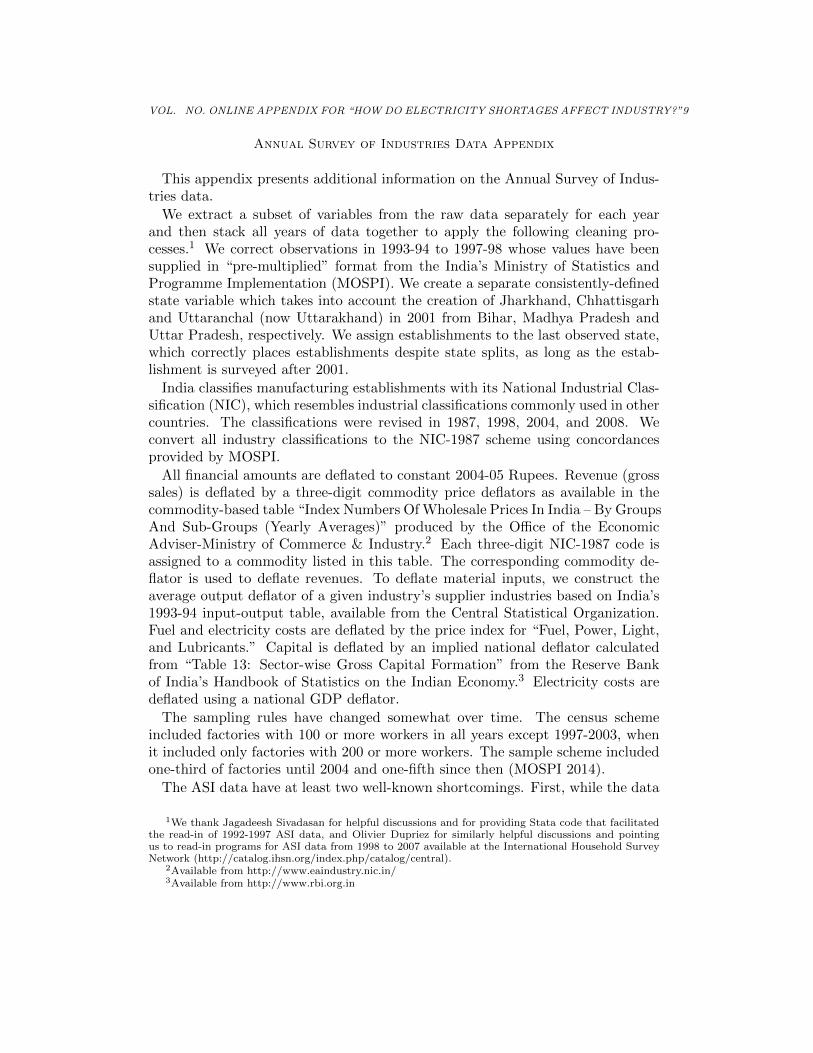
This appendix presents additional information on the Annual Survey of Indus-tries data.We extract a subset of variables from the raw data separately for each year

and then stack all years of data together to apply the following cleaning pro-cesses.1 We correct observations in 1993-94 to 1997-98 whose values have beensupplied in “pre-multiplied” format from the India’s Ministry of Statistics andProgramme Implementation (MOSPI). We create a separate consistently-definedstate variable which takes into account the creation of Jharkhand, Chhattisgarhand Uttaranchal (now Uttarakhand) in 2001 from Bihar, Madhya Pradesh andUttar Pradesh, respectively. We assign establishments to the last observed state,which correctly places establishments despite state splits, as long as the estab-lishment is surveyed after 2001.India classifies manufacturing establishments with its National Industrial Clas-

sification (NIC), which resembles industrial classifications commonly used in othercountries. The classifications were revised in 1987, 1998, 2004, and 2008. Weconvert all industry classifications to the NIC-1987 scheme using concordancesprovided by MOSPI.All financial amounts are deflated to constant 2004-05 Rupees. Revenue (gross

sales) is deflated by a three-digit commodity price deflators as available in thecommodity-based table “Index Numbers Of Wholesale Prices In India – By GroupsAnd Sub-Groups (Yearly Averages)” produced by the O�ce of the EconomicAdviser-Ministry of Commerce & Industry.2 Each three-digit NIC-1987 code isassigned to a commodity listed in this table. The corresponding commodity de-flator is used to deflate revenues. To deflate material inputs, we construct theaverage output deflator of a given industry’s supplier industries based on India’s1993-94 input-output table, available from the Central Statistical Organization.Fuel and electricity costs are deflated by the price index for “Fuel, Power, Light,and Lubricants.” Capital is deflated by an implied national deflator calculatedfrom “Table 13: Sector-wise Gross Capital Formation” from the Reserve Bankof India’s Handbook of Statistics on the Indian Economy.3 Electricity costs aredeflated using a national GDP deflator.The sampling rules have changed somewhat over time. The census scheme

included factories with 100 or more workers in all years except 1997-2003, whenit included only factories with 200 or more workers. The sample scheme includedone-third of factories until 2004 and one-fifth since then (MOSPI 2014).The ASI data have at least two well-known shortcomings. First, while the data

1We thank Jagadeesh Sivadasan for helpful discussions and for providing Stata code that facilitatedthe read-in of 1992-1997 ASI data, and Olivier Dupriez for similarly helpful discussions and pointingus to read-in programs for ASI data from 1998 to 2007 available at the International Household SurveyNetwork (http://catalog.ihsn.org/index.php/catalog/central).

2Available from http://www.eaindustry.nic.in/3Available from http://www.rbi.org.in


are representative of small registered factories and a 100 percent sample of largeregistered factories, not all factories are actually registered under the FactoriesAct. Nagaraj (2002) shows that only 48 percent and 43 percent of the numberof manufacturing establishments in the 1980 and 1990 economic censes appearin the ASI data for those years. Although it is not clear how our results mightdi↵er for unregistered plants, the plants that are observed in the ASI are still asignificant share of plants in India. Second, value added may be under-reported,perhaps associated with tax evasion, by using accounting loopholes to overstateinput costs or under-state revenues (Nagaraj 2002). As long as changes in thisunder-reporting are not correlated with electricity shortages, this will not a↵ectour results.

C1. Determination of Base Sample

Appendix Table A1 details how the sample in Panel B of Table 1 is determinedfrom the original set of observations in the ASI. The 1992-2010 ASI dataset beginswith 949,992 plant-year observations. Plants may still appear in the data evenif they are closed or did not provide a survey response. We drop 172,697 plantsreported as closed or non-responsive. We drop a trivial number of observationsmissing state identifiers and observations in Sikkim, which has only been includedin the ASI sampling frame in the most recent years. We drop 45,664 observationsreporting non-manufacturing NIC codes. We remove a small number of obser-vations (primarily in the early years of our sample) which are exact duplicatesin all fields, assuming these are erroneous multiple entries made from the samequestionnaire form. Due to the importance of revenue and productivity results,we remove the 102,036 observations with missing revenues. We also drop the9,095 observations with two or more input revenue share flags, from the flaggingprocess described below.With this intermediate sample, we use median regression to estimate revenue

productivity (TFPR) under a full Cobb-Douglas model in capital, labor, materi-als, and energy and assuming constant returns to scale. This full Cobb-Douglasrevenue productivity term is used only for the final sample restriction, whichis to drop 4,521 plant-years which have log-TFPR greater than 3.5 in absolutevalue from the sample median. Such outlying TFPR values strongly suggestmisreported inputs or revenues. The final sample includes 615,721 plant-year ob-servations, of which 362,151 are from the sample scheme and 253,570 are fromthe census scheme.

C2. Variable-Specific Sample Restrictions

After the final sample is determined, there may still be observations which havecorrect data for most variables but misreported data for some individual variable.When analyzing specific variables (such as self-generation share, energy revenueshare, or output in Table 6), we therefore additionally restrict the sample usingthe following criteria:


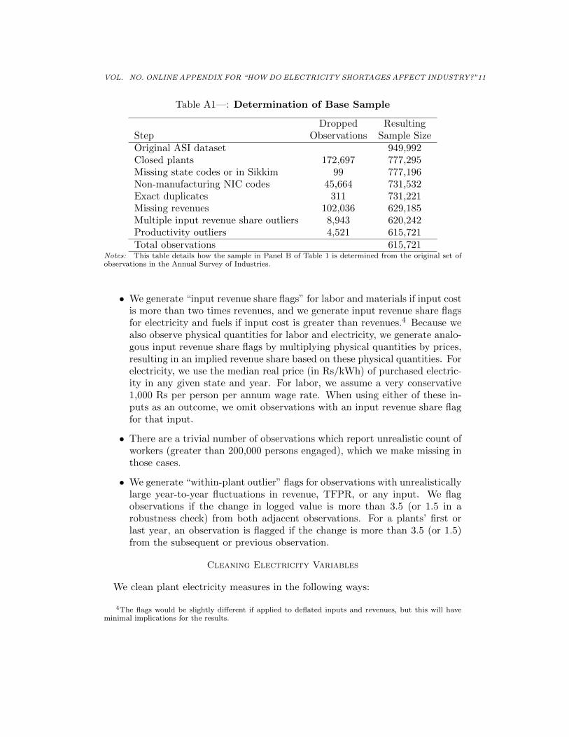
Table A1—: Determination of Base Sample

Dropped ResultingStep Observations Sample SizeOriginal ASI dataset 949,992Closed plants 172,697 777,295Missing state codes or in Sikkim 99 777,196Non-manufacturing NIC codes 45,664 731,532Exact duplicates 311 731,221Missing revenues 102,036 629,185Multiple input revenue share outliers 8,943 620,242Productivity outliers 4,521 615,721Total observations 615,721

Notes: This table details how the sample in Panel B of Table 1 is determined from the original set ofobservations in the Annual Survey of Industries.

• We generate “input revenue share flags” for labor and materials if input costis more than two times revenues, and we generate input revenue share flagsfor electricity and fuels if input cost is greater than revenues.4 Because wealso observe physical quantities for labor and electricity, we generate analo-gous input revenue share flags by multiplying physical quantities by prices,resulting in an implied revenue share based on these physical quantities. Forelectricity, we use the median real price (in Rs/kWh) of purchased electric-ity in any given state and year. For labor, we assume a very conservative1,000 Rs per person per annum wage rate. When using either of these in-puts as an outcome, we omit observations with an input revenue share flagfor that input.

• There are a trivial number of observations which report unrealistic count ofworkers (greater than 200,000 persons engaged), which we make missing inthose cases.

• We generate “within-plant outlier” flags for observations with unrealisticallylarge year-to-year fluctuations in revenue, TFPR, or any input. We flagobservations if the change in logged value is more than 3.5 (or 1.5 in arobustness check) from both adjacent observations. For a plants’ first orlast year, an observation is flagged if the change is more than 3.5 (or 1.5)from the subsequent or previous observation.

Cleaning Electricity Variables

We clean plant electricity measures in the following ways:

4The flags would be slightly di↵erent if applied to deflated inputs and revenues, but this will haveminimal implications for the results.


• We make electricity consumption missing for all observations (other thanbrick kilns) that report zero electricity consumption.

• Wemake all electricity variables missing if the plant reports consuming morethan 110 percent or less than 90 percent of the total amount of electricitythey report purchasing and generating.

• We make missing the values of electricity purchased and sold if the impliedprice per kilowatt-hour is less than 2 percent or more than 5,000 percentof the median grid electricity price calculated across plants in the samestate and year. We also make missing the reported quantities of electricitypurchased and sold if the respective price flag is triggered.

Production Function and Productivity Estimation

We recover production function coe�cients given by Equations (12), (13), and(15) for each of the 143 three-digit industries in the dataset. (To ensure su�cientsample size in each three-digit industry, we adjust industry definitions slightlyto ensure each three-digit industry has at least 100 plant-year observations.) Weuse separate median regression for each two-digit industry, allowing for a lineartime trend and separate intercepts for each underlying three-digit industry. Aftercalculating production function coe�cients, we compute TFPR using Equation(11).For our main TFPR estimates, we define materials to be the plant’s original

reported materials plus fuels not used for self-generation. This latter variable is:Total Fuel Cost - (7 Rs/kWh)⇥(kWh Self-Generated), where 7 Rs/kWh is themedian price reported in the 2005 World Bank Enterprise Survey. This allows usto account for the plant’s full input costs when calculating production functionparameters and TFPR. (In regressions where we use materials as the outcomevariable, we use the original reported materials without adding any fuel costs.)We use several alternative methods for calculating production function coef-

ficients and TFPR for robustness checks, seen in Appendix Table A10. In theorder of that table, these are:

• Including or excluding all fuel costs from the materials variable

• Removing the linear time trend when estimating production coe�cients,which amounts to taking the unconditional median revenue share by indus-try

• Relaxing the assumption that factor shares are constant by plant size, allow-ing all production function coe�cients to vary by plant median ln(Revenue).To implement, we add ln(Revenue) as a term in the median regressions for↵L, ↵M , and ↵E and then segment plants into five size classes when esti-mating ↵K in GMM.


• Backing out the capital coe�cient ↵K under an assumption of constantreturns to scale

• Assuming production is Leontief in electricity and calculating the capitalcoe�cient under an assumption of constant returns to scale. (This is theapproach in our original working paper.)

None of these changes a↵ects the estimated coe�cient by more than about halfof the standard error.


Empirical Strategy Appendix

This appendix presents a table and figures that support the empirical strategysection.

Table A1—: Serial Correlation Tests for the Hydro Instrument

(1) (2)

1st Lag Z 0.107 0.111(0.081) (0.088)

2nd Lag Z 0.008(0.075)

3rd Lag Z -0.130(0.066)**

4th Lag Z -0.104(0.083)

5th Lag Z -0.025(0.068)

Number of Obs. 540 420F-Stat 1.72 1.90R-Squared 0.01 0.07

Notes: This table presents regressions of the hydro instrument Zst on its lags. Robust standard errors.*,**, ***: Statistically di↵erent from zero with 90, 95, and 99 percent confidence, respectively.


Figure A1. : Shortages and Hydro Generation in Karnataka

0.2

.4.6

.8

1990 1995 2000 2005 2010year

Shortage Hydro Generation/Total Consumption

Notes: Shortage data are estimated by the Central Electricity Authority. Hydro Generation/TotalElectricity Consumption is a simplified version of the hydro availability instrument. The figure gives asimple graphical example of the first stage of our IV estimator.


Figure A2. : Rainfall and Hydro Share of Electricity by State

Andaman and Nicobar Islands

Andhra Pradesh

Assam

Bihar

Chandigarh

CG

Delhi

GA

GujaratHaryana

Himachal Pradesh

Jammu and Kashmir

Karnataka

Kerala

Madhya PradeshMH

Manipur

Meghalaya

Nagaland

Orissa

Punjab

Rajasthan

Tamil Nadu

Tripura

UP

UK

West Bengal

01

23

419

92-2

010

Mea

n Ra

infa

ll (m

eter

s)

0 .5 11992-2010 Mean of Hydro Generation/Total Consumption

Notes: This figure plots sample average annual rainfall against the mean ratio of hydroelectricitygeneration to total electricity consumption. The figure emphasizes that there is substantial variation inhydro generation conditional on rainfall.


Figure A3. : Hydro Share of Predicted Consumption Over Time in FiveLarge States

0.2

.4.6

Hyd

ro G

ener

atio

n/Pr

edic

ted

Con

sum

ptio

n

1990 1995 2000 2005 2010

Andhra Pradesh GujaratKarnataka Uttar PradeshWest Bengal India Average

Notes: This figure presents the ratio of hydro generation to predicted consumption over 1992-2010 forfive large states. Di↵erent states have di↵erent slopes, illustrating the importance of including state-specific time trends as control variables.


Figure A4. : ln(Energy Available) Over Time in Five Large States

9.5

1010

.511

11.5

ln(E

nerg

y Av

aila

ble)

1990 1995 2000 2005 2010

Andhra Pradesh GujaratKarnataka Uttar PradeshWest Bengal

Notes: This figure presents the natural log of Energy Available over 1992-2010 for five large states.Di↵erent states have di↵erent slopes, illustrating the importance of including state-specific time trendsas control variables.


Robustness Checks for Tables 6 and 7

This appendix presents robustness checks for Tables 6 and 7. We first presentestimates from the di↵erence estimator. We then present a series of robustnesschecks for the fixed e↵ects estimator, including alternative weather controls, al-ternative instruments, and alternative constructions of TFPR.

E1. Estimates with Di↵erence Estimator

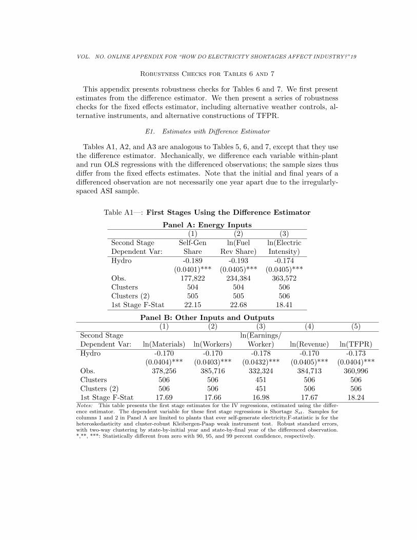
Tables A1, A2, and A3 are analogous to Tables 5, 6, and 7, except that they usethe di↵erence estimator. Mechanically, we di↵erence each variable within-plantand run OLS regressions with the di↵erenced observations; the sample sizes thusdi↵er from the fixed e↵ects estimates. Note that the initial and final years of adi↵erenced observation are not necessarily one year apart due to the irregularly-spaced ASI sample.

Table A1—: First Stages Using the Di↵erence Estimator

Panel A: Energy Inputs(1) (2) (3)

Second Stage Self-Gen ln(Fuel ln(ElectricDependent Var: Share Rev Share) Intensity)Hydro -0.189 -0.193 -0.174

(0.0401)*** (0.0405)*** (0.0405)***Obs. 177,822 234,384 363,572Clusters 504 504 506Clusters (2) 505 505 5061st Stage F-Stat 22.15 22.68 18.41

Panel B: Other Inputs and Outputs(1) (2) (3) (4) (5)

Second Stage ln(Earnings/Dependent Var: ln(Materials) ln(Workers) Worker) ln(Revenue) ln(TFPR)Hydro -0.170 -0.170 -0.178 -0.170 -0.173

(0.0404)*** (0.0403)*** (0.0432)*** (0.0405)*** (0.0404)***Obs. 378,256 385,716 332,324 384,713 360,996Clusters 506 506 451 506 506Clusters (2) 506 506 451 506 5061st Stage F-Stat 17.69 17.66 16.98 17.67 18.24

Notes: This table presents the first stage estimates for the IV regressions, estimated using the di↵er-ence estimator. The dependent variable for these first stage regressions is Shortage Sst. Samples forcolumns 1 and 2 in Panel A are limited to plants that ever self-generate electricity.F-statistic is for theheteroskedasticity and cluster-robust Kleibergen-Paap weak instrument test. Robust standard errors,with two-way clustering by state-by-initial year and state-by-final year of the di↵erenced observation.*,**, ***: Statistically di↵erent from zero with 90, 95, and 99 percent confidence, respectively.


Table A2—: E↵ects of Shortages on Energy Inputs Using the Di↵erenceEstimator

(1) (2) (4)Self-Gen ln(Fuel ln(Electric

Dependent Var: Share Rev Share) Intensity)Panel A: OLS

Shortage 0.274 0.874 -0.595(0.0383)*** (0.202)*** (0.132)***

Panel B: IVShortage 0.349 2.419 0.339

(0.135)*** (0.713)*** (0.724)Obs. 177,822 234,384 363,572Clusters 504 504 506Clusters (2) 505 505 5061st Stage F-Stat 22.15 22.68 18.41

Notes: This table presents estimates of Equation (21) using the di↵erence estimator. Panel B instru-ments for Shortage using hydro availability. Samples for columns 1 and 2 are limited to plants that everself-generate electricity. F-statistic is for the heteroskedasticity and cluster-robust Kleibergen-Paap weakinstrument test. Robust standard errors, with two-way clustering by state-by-initial year and state-by-final year of the di↵erenced observation. *,**, ***: Statistically di↵erent from zero with 90, 95, and 99percent confidence, respectively.

Table A3—: E↵ects of Shortages on Materials, Labor, Revenue, andTFPR Using the Di↵erence Estimator

(1) (2) (3) (4) (5)ln(Earnings/

Dependent Var: ln(Materials) ln(Workers) Worker) ln(Revenue) ln(TFPR)Panel A: OLS

Shortage 0.0203 0.0254 0.201 0.158 0.0724(0.0841) (0.0526) (0.0508)*** (0.0762)** (0.0394)*

Panel B: IVShortage -0.959 -0.397 -0.243 -0.828 -0.106

(0.460)** (0.315) (0.224) (0.491)* (0.238)Obs. 378,256 385,716 332,324 384,713 360,996Clusters 506 506 451 506 506Clusters (2) 506 506 451 506 5061st Stage F-Stat 17.69 17.66 16.98 17.67 18.24

Notes: This table presents estimates of Equation (21) using the di↵erence estimator. Panel B instru-ments for Shortage using hydro availability. F-statistic is for the heteroskedasticity and cluster-robustKleibergen-Paap weak instrument test. Robust standard errors, with two-way clustering by state-by-initial year and state-by-final year of the di↵erenced observation. *,**, ***: Statistically di↵erent fromzero with 90, 95, and 99 percent confidence, respectively.


E2. Robustness Checks

This section presents robustness checks for Tables 6 and 7. Tables are organizedseparately for each of the main outcomes for ease of comparison. Column 1excludes industry-by-year e↵ects µjt. Column 2 uses a tolerance of 1.5 natural logsin the outlier flagging process described in Online Appendix C.C2, while column 3does not exclude any flagged outliers. Columns 4 and 5 use ln(Energy Available)and Peak Shortage, respectively, instead of Shortage. Column 6 clusters standarderrors by state.We make two explanatory comments. First, the first stage F-statistics for

ln(Energy Available) in column 4 are smaller than when using Shortage as the en-dogenous variable in the main estimates, which is unsurprising: unlike Shortage,ln(Energy Available) grows monotonically within states over the sample, and thestate-specific linear time trends st do not control very well for di↵erent states’actual growth rates. Second, the first stage F-statistics increase in two specifica-tions when clustering by state in column 6, and this may be a small sample biasfrom having only 30 state-level clusters.


Table A4—: Robustness Checks: Energy Inputs

(1) (2) (3) (4) (5) (6)No Ind.- Tighter No Use Use Clusterby-Year Outlier Outlier ln(Energy Peak by

Change from Base Spec: E↵ects µjt Flags Flags Available) Shortage StateSelf-Generation Share

Shortage 0.455 0.394 0.450 0.433 0.404 0.442(0.156)*** (0.141)*** (0.158)*** (0.163)*** (0.169)** (0.129)***

Number of Obs. 240,743 223,128 293,866 240,743 240,743 240,743First Stage F-Stat 15.08 16.97 17.02 9.285 9.705 35.12

ln(Fuel Revenue Share)Shortage 3.675 2.700 3.022 3.133 3.107 3.294

(1.158)*** (1.001)*** (1.298)** (1.215)*** (1.274)** (0.961)***Number of Obs. 291,759 268,663 300,697 291,759 291,759 291,759First Stage F-Stat 14.79 16.49 16.56 9.829 8.773 37.85

ln(Electric Intensity)Shortage -0.177 -0.0320 0.0247 0.0764 0.0726 0.0926

(0.735) (0.708) (0.753) (0.616) (0.591) (0.694)Number of Obs. 479,616 453,482 483,843 479,616 479,616 479,616First Stage F-Stat 13.89 14.86 14.99 13.71 11.38 13.41

Notes: This table presents alternative estimates for Table 6, instrumenting for Shortage using hydroavailability. Samples for the first two panels are limited to plants that ever self-generate electricity. F-statistic is for the heteroskedasticity and cluster-robust Kleibergen-Paap weak instrument test. Robuststandard errors, with two-way clustering by plant and state-year. *,**, ***: Statistically di↵erent fromzero with 90, 95, and 99 percent confidence, respectively.


Table A5—: Robustness Checks: Materials, Labor, Revenue, and TFPR

(1) (2) (3) (4) (5) (6)No Ind.- Tighter No Use Use Clusterby-Year Outlier Outlier ln(Energy Peak by

Change from Base Spec: E↵ects µjt Flags Flags Available) Shortage Stateln(Materials)

Shortage -1.048 -1.017 -1.237 -0.917 -0.915 -1.137(0.548)* (0.472)** (0.595)** (0.392)** (0.433)** (0.561)**

Number of Obs. 495,043 478,152 498,464 495,043 495,043 495,043First Stage F-Stat 13.20 14.20 14.22 13.91 10.29 12.52

ln(Workers)Shortage -0.230 -0.253 -0.248 -0.195 -0.196 -0.243


ln(Earnings/Worker)Shortage -0.321 -0.384 -0.367 -0.234 -0.260 -0.267

(0.239) (0.220)* (0.244) (0.180) (0.241) (0.243)Number of Obs. 456,443 440,524 461,131 456,443 456,443 456,443First Stage F-Stat 13.45 14.76 14.45 12.49 7.354 9.508

ln(Revenue)Shortage -1.050 -0.993 -1.255 -0.877 -0.880 -1.091

(0.555)* (0.494)** (0.638)** (0.385)** (0.458)* (0.646)*Number of Obs. 501,130 484,753 503,664 501,130 501,130 501,130First Stage F-Stat 13.13 14.02 14.19 14.04 10.22 12.45

ln(TFPR)Shortage -0.0733 -0.246 -0.408 -0.247 -0.242 -0.304


Notes: This table presents alternative estimates for Table 7, instrumenting for Shortage using hydroavailability. F-statistic is for the heteroskedasticity and cluster-robust Kleibergen-Paap weak instrumenttest. Robust standard errors, with two-way clustering by plant and state-year. *,**, ***: Statisticallydi↵erent from zero with 90, 95, and 99 percent confidence, respectively.


E3. Alternative Weather Controls

This section presents estimates of Tables 6 and 7 with alternative weathercontrols. Column 1 controls linearly for rainfall instead of including rainfall bins.Columns 2 and 3 use 100mm and 50 mm rainfall bins, respectively, instead of60mm bins. Column 4 uses rainfall data from the National Climate Centre insteadof the University of Delaware.

Table A6—: Alternative Weather Controls: Energy Inputs

(1) (2) (3) (4)100mm 50mm NCC

Linear Rainfall Rainfall RainfallChange from Base Spec: Rainfall Bins Bins Data

Self-Generation ShareShortage 0.412 0.458 0.442 0.406

(0.175)** (0.155)*** (0.153)*** (0.150)***Rainfall 0.00130

(0.00892)First Stage F-Stat 16.12 19.05 17.00 21.63

ln(Fuel Revenue Share)Shortage 2.797 3.049 3.294 1.901

(1.052)*** (0.934)*** (1.032)*** (0.826)**Rainfall 0.185

(0.0663)***First Stage F-Stat 15.41 18.20 16.53 20.98

ln(Electric Intensity)Shortage -0.0294 0.0583 0.0926 0.0894

(0.775) (0.696) (0.755) (0.665)Rainfall -0.0264


Notes: This table presents alternative estimates for Table 6, instrumenting for Shortage using hydroavailability. Samples for the first two panels are limited to plants that ever self-generate electricity. F-statistic is for the heteroskedasticity and cluster-robust Kleibergen-Paap weak instrument test. Robuststandard errors, with two-way clustering by plant and state-year. *,**, ***: Statistically di↵erent fromzero with 90, 95, and 99 percent confidence, respectively.


Table A7—: Alternative Weather Controls: Materials, Labor, Revenue,and TFPR

(1) (2) (3) (4)100mm 50mm NCC

Linear Rainfall Rainfall RainfallChange from Base Spec: Rainfall Bins Bins Data

ln(Materials)Shortage -0.969 -1.014 -1.137 -0.915

(0.481)** (0.431)** (0.511)** (0.426)**Rainfall -0.0118


ln(Workers)Shortage -0.219 -0.228 -0.243 -0.249

(0.337) (0.301) (0.339) (0.297)Rainfall 0.00649


ln(Earnings/Worker)Shortage -0.181 -0.214 -0.267 -0.189

(0.206) (0.191) (0.218) (0.190)Rainfall 0.00188


ln(Revenue)Shortage -0.913 -0.988 -1.091 -0.792

(0.504)* (0.456)** (0.536)** (0.433)*Rainfall -0.0262


ln(TFPR)Shortage -0.299 -0.294 -0.304 -0.235

(0.254) (0.232) (0.259) (0.221)Rainfall -0.0142


Notes: This table presents alternative estimates for Table 7, instrumenting for Shortage using hydroavailability. F-statistic is for the heteroskedasticity and cluster-robust Kleibergen-Paap weak instrumenttest. Robust standard errors, with two-way clustering by plant and state-year. *,**, ***: Statisticallydi↵erent from zero with 90, 95, and 99 percent confidence, respectively.


E4. Alternative Instruments

This section presents estimates of Tables 6 and 7 with alternative instruments.Column 1 replicates the base estimates except using actual hydro generationinstead of generation predicted from reservoirs and run-of-river plants. Columns2 and 3 add Nst, the predicted generation from plants that came online in theprevious year, as an additional supply shifter to increase power. Because Indianstates are still not large compared to generation from a single plant, new plantsgenerate lumpy reductions in shortages the year they come online. Power plantshave a long and potentially unpredictable time-to-build, so we assume that theyear that a plant comes online is exogenous conditional on state trends. Theinstrument in columns 2 and 3 is:

(E1) Zst =Hst +Nst

Q̃st.

To get Nst, we simply multiply the capacity added in the previous year bythe national average thermal plant capacity factor in year t. Column 2 uses Hst

from reservoirs and run-of-river plants (as in the base estimates), while column 3instead uses actual hydro generation (as in column 1).The results below show that adding Nst provides a moderate increase in preci-

sion but does not otherwise change the results. We used this in an earlier workingpaper version, although it does not appear in the body of the published versiondue to concerns about the exogeneity of Nst.


Table A8—: Alternative Instruments: Energy Inputs

(1) (2) (3)Base With New Supply

Actual Predicted with ActualHydro Run-of-River Hydro

Instrument: Generation and Reservoirs GenerationSelf-Generation Share

Shortage 0.794 0.463 0.788(0.176)*** (0.142)*** (0.167)***

Number of Obs. 240,743 240,743 240,743First Stage F-Stat 17.61 19.74 19.44

ln(Fuel Revenue Share)Shortage 3.597 3.318 3.596

(1.049)*** (0.955)*** (1.003)***Number of Obs. 291,759 291,759 291,759First Stage F-Stat 17.76 19.36 19.72

ln(Electric Intensity)Shortage -1.392 0.173 -1.217

(0.718)* (0.698) (0.673)*Number of Obs. 479,616 479,616 479,616First Stage F-Stat 14.24 17.73 16.18

Notes: This table presents estimates of Table 6 with alternative instruments. Samples for the first twopanels are limited to plants that ever self-generate electricity. F-statistic is for the heteroskedasticity andcluster-robust Kleibergen-Paap weak instrument test. Robust standard errors, with two-way clusteringby plant and state-year. *,**, ***: Statistically di↵erent from zero with 90, 95, and 99 percent confidence,respectively.


Table A9—: Alternative Instruments: Materials, Labor, Revenue, andTFPR

(1) (2) (3)Base With New Supply

Actual Predicted with ActualHydro Run-of-River Hydro

Instrument: Generation and Reservoirs Generationln(Materials)

Shortage -1.370 -1.216 -1.415(0.607)** (0.473)** (0.576)**

Number of Obs. 495,043 495,043 495,043First Stage F-Stat 13.88 17.05 15.89

ln(Workers)Shortage -0.232 -0.302 -0.280

(0.356) (0.313) (0.341)Number of Obs. 502,724 502,724 502,724First Stage F-Stat 13.82 16.99 15.82

ln(Earnings/Worker)Shortage -0.542 -0.225 -0.487

(0.270)** (0.199) (0.247)**Number of Obs. 456,443 456,443 456,443First Stage F-Stat 13.25 17.09 15.07

ln(Revenue)Shortage -1.019 -1.182 -1.097

(0.586)* (0.498)** (0.560)*Number of Obs. 501,130 501,130 501,130First Stage F-Stat 13.84 16.95 15.83

ln(TFPR)Shortage 0.158 -0.297 0.128

(0.274) (0.236) (0.257)Number of Obs. 479,313 479,313 479,313First Stage F-Stat 14.21 17.75 16.22

Notes: This table presents estimates of Table 6 with alternative instruments. F-statistic is for theheteroskedasticity and cluster-robust Kleibergen-Paap weak instrument test. Robust standard errors,with two-way clustering by plant and state-year. *,**, ***: Statistically di↵erent from zero with 90, 95,and 99 percent confidence, respectively.


E5. Alternative TFPR Measures

Table A10 presents estimates of Equation (21), using alternative measures ofTFPR described in Appendix C.C2.

Table A10—: Robustness Check: Estimates with Alternative TFPRMeasures

(1) (2) (3) (4) (5) (6)Include Include No Time ↵ Varies LeontiefAll Fuels No Fuels Trend by Size CRS CRS

Shortage -0.285 -0.150 -0.097 -0.112 -0.110 -0.211(0.240) (0.248) (0.211) (0.212) (0.221) (0.266)

Number of Obs. 479,609 479,484 480,100 494,210 479,755 477,720Number of Clusters 112,405 112,330 112,472 115,015 112,397 112,014Number of Clusters (2) 536 536 536 536 536 536

First Stage F-Stat 14.87 14.88 14.84 14.32 14.85 14.89Notes: F-statistic is for the heteroskedasticity and cluster-robust Kleibergen-Paap weak instrumenttest. Robust standard errors, with two-way clustering by plant and state-year. *,**, ***: Statisticallydi↵erent from zero with 90, 95, and 99 percent confidence, respectively.


E6. Heterogeneous E↵ects of Shortages

Table A11 presents estimates of heterogeneous e↵ects of shortages for plantswith generators and for plants in industries with above-median electric intensity.Denote Mi as a 3-by-1 vector of these two moderators and a constant. Theestimating equation is identical to Equation 21 except with Mi interacted withall right-hand-side variables other than µjt.Table A11 presents the estimated interactions with the Shortage variable. As

expected, column 2 shows that self-generators increase fuel use more when short-ages worsen, while non-generators do not. However, we do not have the power todetect heterogeneous e↵ects on revenues or TFPR. As a benchmark, in the WorldBank Enterprise Survey, generators and non-generators report 7.3 and 8.4 per-cent losses from power cuts, respectively - a ratio of 8.4/7.3⇡1.15. Our revenueestimates are statistically indistinguishable from this benchmark ratio.These empirical results are not interpretable as the average causal e↵ects of gen-

erator ownership, because endogenous generator adoption decisions could implythat the plants without generators have unobservably smaller losses. For exam-ple, plants without generators might have unobservably better electricity supply,reducing their losses from not adopting generators and also reducing the e↵ectsof an increase in shortages.

Table A11—: Heterogeneous E↵ects of Shortages

(1) (2) (3) (4)Self-Gen ln(Fuel

Dependent Variable: Share Rev Share) ln(Revenue) ln(TFPR)

Shortage -0.027 -0.867 -0.478 -0.201(0.065) (1.748) (0.695) (0.445)

Shortage x Elec Intensive 0.022 0.189 -0.936 0.130(0.131) (2.181) (1.212) (0.551)

Shortage x Self-Generator 0.470 4.050 -0.384 -0.413(0.155)*** (1.956)** (0.716) (0.386)

Number of Obs. 428,969 477,005 501,130 479,313Number of Clusters 102,995 109,715 116,231 112,371Number of Clusters (2) 536 536 536 536

Notes: Robust standard errors, with two-way clustering by plant and state-year. *,**, ***: Statisticallydi↵erent from zero with 90, 95, and 99 percent confidence, respectively.


Simulation Appendix

This appendix presents full detail on the simulations, as well as additionalrobustness checks using di↵erent assumed production functions.

F1. Simulation Inputs

Table A1 presents the sources of the parameters used in the simulations.

Table A1—: Simulation Inputs

Parameter Source Level↵K , ↵L, ↵M , ↵E Production function estimates from ASI Industry Level� Shortage Sst from CEA or other assumed value State-YearGenerator ownership Inferred from non-zero electricity generation in ASI PlantK Capital stock in ASI Plant-Year⌦ Estimated revenue productivity Plant-YearpM , pL, p Normalized to 1 ConstantpE,G=4.5 Rs/kWh Median grid electricity price from WBES ConstantpE,S=7 Rs/kWh Median self-generated electricity cost from WBES Constant

Notes: WBES refers to the 2005 World Bank Enterprise Survey.

F2. Exogenous Generators: Cobb-Douglas

This section presents full details on how the simulations in Section VI de-termine optimal input and output bundles conditional on exogenous generatorownership. Here we present the Cobb-Douglas model in Section III; subsequentsections present alternative models (Leontief and Constant Elasticity of Substi-tution).The procedure takes production function parameters {↵E ,↵L,↵M ,↵K} and

exogenous state variables capital Kit, productivity ⌦it, and shortages �it. Theoptimal input choices of labor and materials are solved using profit maximizationconditions, and L⇤, M⇤G, M⇤S , E⇤G, E⇤S , and R⇤ are determined (where thesuperscripts S and G refer to shortage and non-shortage – grid – respectively) .This procedure is repeated for each plant i observed in the ASI data.

1) Plants without generators

The optimal input bundles can be found analytically, using the first-orderconditions. Non-generators shut down during outages, so MS = ES = 0.The first-order condition for materials during non-outage periods, @⇡it⌧

@Mit⌧=

0, yields

(F1) ↵M⌦K↵K [MG]↵M�1L↵L [EG]↵E = pM .


Analogously, the FOC for electricity, @⇡it⌧@Eit⌧

= 0, yields

(F2) ↵E⌦K↵K [MG]↵ML↵L [EG]↵E�1 = pE,G.

Finally, the FOC for labor, @⇡it@Lit

= 0 yields

(F3) ↵L(1� �)⌦K↵K [MG]↵ML↵L�1[EG]↵E = pL.

Rearranging these three equations, we obtain:

M⇤G =

"⌦K↵K

✓↵M

pM

◆1�↵L�↵E✓(1� �)↵L

pL

◆↵L✓

↵E

pE,G

◆↵E# 1

1�↵L�↵M�↵E

L⇤ = (1� �)pM↵L

pL↵MM⇤G

E⇤G =pM↵E

pE↵MM⇤G

(F4)

Annual revenue is thus:

R = (1� �)⌦K↵K [M⇤G]↵M [L⇤]↵L [E⇤G]↵E

Notice that if there are no shortages; � = 0, the same equations can alsobe used to determine optimal input bundles for all plants (assuming thatpE,G < pE,S).

2) Plants with generators

There are five first-order conditions, @⇡it⌧

@MSit⌧

= 0, @⇡it⌧

@MGit⌧

= 0, @⇡it⌧

@ESit⌧

= 0,@⇡it⌧

@EGit⌧

= 0, and @⇡it@Lit

= 0. These yield

↵M⌦K↵K [MG]↵M�1L↵L [EG]↵E = pM

↵M⌦K↵K [MS ]↵M�1L↵L [ES ]↵E = pM

↵M⌦K↵K [MS ]↵ML↵L [ES ]↵E�1 = pE,S

↵M⌦K↵K [MG]↵ML↵L [EG]↵E�1 = pE,G

↵L(1� �)⌦K↵K [MG]↵ML↵L�1[EG]↵E

+↵L�p⌦K↵K [MS ]↵ML↵L�1[ES ]↵E = pL

(F5)

The set of equations in system (F5) are solved numerically in MATLABusing the fsolve routine. Rather than solving for L⇤, E⇤G, E⇤,S , M⇤G, and


M⇤S in levels, we solve in logarithms, since these values can di↵er by severalorders of magnitude for di↵erent plants in the data. The starting values forL⇤, E⇤G, E⇤S , M⇤G, andM⇤S are given by the analytic values from equation(F4), the no-shortage values.

Annual revenue is:

R =(1� �)⌦K↵K [M⇤G]↵M [L⇤]↵L [E⇤G]↵E

+ �⌦K↵K [M⇤S ]↵M [L⇤]↵L [E⇤S ]↵E

F3. Exogenous Generators: Leontief in Electricity

Our original working paper used production functions that were Leontief inelectricity and a Cobb-Douglas aggregate of capital, labor, and materials. Forcomparison, we include this below.Denoting physical productivity as A, the physical production function is:

(F6) Q = min{AK↵KL↵LM↵M ,1

�E}

The Leontief production function dictates that electricity is used in constantproportion 1

� with output. Electricity intensity � varies across industries. HavingA inside the Cobb-Douglas aggregator ensures that electricity is used in fixedproportion to output instead of to the bundle of other inputs.Since we will observe total revenues rather than physical quantities produced,

we need to relate revenues to our production function in equation (F6). Weassume that plants sell into a perfectly competitive output market with price p,and denote ⌦ ⌘ pA.Firms have the following daily profit function ⇧it⌧ :

⇧it⌧ =pmin{AitK↵Kit L↵L

it M↵Mit⌧ ,

1

�Eit⌧}

� pLLit � pMMit⌧ � pEEit⌧ ,(F7)

where pL pM are the prices of labor and materials, respectively. Capital is ex-cluded, as it is sunk before the plant makes any production decisions.Given the Leontief-in-electricity structure of production, cost minimization im-

plies that for any desired level of output Q, the firm produces at a “corner” ofthe isoquant where:

(F8) AitK↵Kit L↵L

it M↵Mit⌧ =

1

�Eit⌧ ,

Given this, one can rewrite the profit function, substituting in ⌦it and the


optimized value of electricity:

⇧it⌧ = (1� �pE

p)⌦itAitK

↵Kit L↵L

it M↵Mit⌧ � pLLit � pMMit⌧(F9)

Let � ⌘ �pE,G

p = pE,GEit⌧pQit⌧

= pE,GEitRit

, the electricity revenue share if a firm only

uses electricity purchased from the grid. Notice that if (1� �) < 0, then the firmwill choose not to produce.There are three cases that can occur, depending on electricity intensity and the

relative price of electricity:

1) If p > �pE,S , the plant always produces, regardless of power outages.

2) If �pE,S > p > �pE,G, the plant does not produce during power outages,but does produce otherwise.

3) If p < �pE,G, the plant never produces.

We ignore case (3): if plants never produce, they never appear in the data. Plantswithout generators e↵ectively have pE,S = 1, so case (1) cannot arise. Of theplants with generators, those with higher � will be in case (2). In other words,higher-electricity intensity plants will be more likely to shut down during gridpower outages.5

The first-order condition with respect to materials yields:

(F10) ↵M (1� �)Rit⌧

Mit⌧� pM = 0.

The marginal revenue product of materials is:

(F11) MRPM =

(↵M (1� �) Rit⌧

Mit⌧if grid power

T ↵M (1� �) Rit⌧Mit⌧

if power outage

When setting labor, the firm begins with its yearly profit function, which issimply the weighted average of Equation (F9) over grid power and outage periods.If a plant is in case (1), meaning that it self-generates during power outages, thenthe first-order condition is given by:

(F12) MRPL = ↵L(1� �)

(1� �)

RGit

Lit+ �T RS

it

Lit

�= pL,

where RSit and RG

it indicate revenues during outage and grid power periods, re-spectively.

5While a firm would not invest in a generator if it expected to be in case (2), unexpected changes inp, pE,S , or pE,G could cause firms with generators to not use them.


We now solve for profit-maximizing inputs and output. Define �G ⌘ �pE,G

p and

�S ⌘ �pE,S

p .

1) If in Case 3:

The plant never produces. Thus L⇤ = M⇤G = M⇤S = E⇤G = E⇤S = R⇤ =0.

2) If in Case 2 (including non-generators with �G < 1):

The plant operates when there is grid power, but not during an outage.The optimal input bundles can be found analytically, using the first-orderconditions. Clearly, M⇤S = 0. The FOC for materials during grid powerperiods, @⇡it⌧

@Mit⌧= 0, yields

(F13) ↵M (1� �G)⌦K↵K [MG]↵M�1L↵L = pM .

The FOC for labor, @⇡it@Lit

= 0 yields

(F14) ↵L(1� �G)(1� �)⌦K↵K [MG]↵ML↵L�1 = pL.

Rearranging these first-order equation, we obtain

M⇤G =

"(1� �)⌦K↵K

✓↵M

pM

◆1�↵L✓(1� �)↵L

pL

◆↵L# 1

1�↵L�↵M

L⇤ = (1� �)pM↵L

pL↵MM⇤G

.(F15)

Given labor and material choices, it is straightforward to compute revenue:

R = ⌦K↵K [M⇤G]↵M [L⇤]↵L .

Electricity consumption is:E⇤G = �SR

Notice that if there are no shortages; � = 0, the same equations can also beused to get optimal input bundles and revenue for all plants.

3) If in Case 1 (plants with generators only):

The plant always operates, running its generator during outages. There arethree first-order conditions, @⇡it⌧

@MSit⌧

= 0, @⇡it⌧

@MGit⌧

= 0, and @⇡it@Lit

= 0.


↵M (1� �G)p⌦K↵K [MG]↵M�1L↵L = pM

↵M (1� �S)p⌦K↵K [MS ]↵M�1L↵L = pM

↵L(1� �G)(1� �)p⌦K↵K [MG]↵ML↵L�1

+↵L�(1� �S)p⌦K↵K [MS ]↵ML↵L�1 = pL

(F16)

The system of equations in (F16) is solved numerically in MATLAB usingthe fsolve routine.

Finally, electricity usage is

E⇤G = (1� �)�G⌦K↵K [M⇤G]↵M [L⇤]↵L

E⇤S = ��S⌦K↵K [M⇤G]↵M [L⇤]↵L .

Annual revenue is:

R =(1� �)⌦K↵K [M⇤G]↵M [L⇤]↵L

+ �⌦K↵K [M⇤S ]↵M [L⇤]↵L

F4. Exogenous Generators: Constant Elasticity of Substitution

One issue with the production functions that we have considered is that thereis no direct intertemporal substitution in production. Suppose instead that weconsider a CES aggregator with constant elasticity of substitution � between daysgiven by:

Rit =

ˆ⌧(Rit⌧ )

�d⌧

� 1�

Notice that this is a CES type aggregator, so there is symmetric substitutionacross all days of the year. If � = 1, we have the process considered in the paper.If � < 1, outputs are interday complements, and if � > 1, then there is inter-daysubstitution.

Given that in the daily production function, only materials and electricity canbe varied, we can think of the daily production function as being written as:

Rit = ⌦itK↵Kit L↵L

it

ˆ⌧Eit⌧

�↵EMit⌧�↵Md⌧

� 1�

Notice that the daily returns to scale in the production function will be givenby �(↵M + ↵E), an issue we return to below.


First-Order Conditions for Non-Generators

For firms that do not have generators, revenue is:

Rit =

ˆ⌧(Rit⌧ )

�d⌧

� 1�

= [(1� �)M�↵Mit⌧ E�↵E

it⌧ L�↵Lit K�↵K

it ]1�

= (1� �)1�M↵M

it⌧ L↵Lit E↵E

it⌧ K↵Kit

= (1� �)1�

✓Mit

(1� �)

◆↵M✓

Eit

(1� �)

◆↵E

L↵Lit K↵K

it

= (1� �)1��↵M�↵EM↵M

it E↵Eit L↵L

it K↵Kit

(F17)

where we have assumed that the same input choice will be optimal across daysto go from the first to the second line of this equation. Notice that shortages cancause anything between a zero and infinite decrease in revenues by changing �,holding inputs fixed. Thus, our predictions are not robust to a range of �. More-over, the only di↵erence between this setup and the setup without intertemporal

substitution is that the plant’s revenue decreases by (1 � �)1��↵M�↵E instead of

(1� �)1�↵M�↵E .

First-Order Conditions for Generators

The profit function is:

(F18) ⇧it = Rit � pMˆ⌧Mit⌧d⌧ � pE

ˆ⌧Eit⌧d⌧ � pL

ˆ⌧Lit⌧d⌧

For plants with generators, the materials first-order condition, @⇧it@Mit⌧

= 0, yields

(F19)1

�R

1��11�

it �↵MR�

it⌧

Mit⌧= pM .

The electricity FOC is similar:

(F20)1

�R

1��11�

it ↵ER�

it⌧

Eit⌧= pE .


The labor FOC, @⇧it@Lit

= 0, yields:

(F21)1

�R

1��11�

it �↵L

"(1� �)

�RG

it

��

Lit⌧+ �

�RS

it

��

LSit⌧

#= pL,

where RGit = ⌦L↵L(MG)↵M (EG)↵EK↵K and RS

it = ⌦L↵L(MS)↵M (ES)↵EK↵K .The set of the equations (F19,F20,F21) are solved numerically in MATLAB usingthe fsolve routine. Rather than solving for L⇤, E⇤G, E⇤,S , M⇤G, and M⇤S inlevels, we solve in logarithms.

F5. Comparing Predictions from Cobb-Douglas, Leontief, and CES Models

Table A2 presents the simulated e↵ects of the 2005 assessed Shortage levelsSs2005 relative to zero shortage. Indeed, Table A2 replicates Panel A of Table9. Column 1 shows the Cobb-Douglas production function used in the body ofthe paper. Column 2 presents the Leontief model, while columns 3 and 4 presentresults of the CES model with � = 0.9 and � = 0.5, respectively.6 The predic-tions from the Cobb-Douglas and Leontief model are virtually identical, despitethe di↵erent functional forms and di↵erent approaches to production function es-timation. In the CES model, simulated losses are almost identical for plants withgenerators, but much larger for non-generators.

Table A2—: Predictions from Di↵erent Production Function Models

Cobb-Douglas Leontief CES � = 0.9 CES � = 0.5(1) (2) (3) (3)

Revenue Loss: Average 5.6% 5.7% 7.5% 18%Revenue Loss: Non-Generators 10.0% 9.8% 13% 32%Revenue Loss: Generators 0.4% 0.6% 0.4% 0.4%

TFPR Loss: Average 1.5% 1.3% 1.9% 5.8%TFPR Loss: Non-Generators 2.6% 2.4% 3.5% 10.6%TFPR Loss: Generators 0.0% 0.0% 0.0% 0.0%

Notes: This table presents the e↵ects of the 2005 assessed Shortage levels relative to zero Shortage.Cobb-Douglas, Leontief, and CES, refer to the production functions used for estimation and prediction,and are described in text.

6Using a higher value of � such as � = 1.5 yields the implication that a firm will have increasingreturns at the daily level, since the returns to scale in the daily production function are �(↵M + ↵E),so �(↵M + ↵E) > 1 means that it is optimal to produce all output on a single day of the year. For theCES simulation, we use production function coe�cients ↵E , ↵L, ↵M , ↵K , and ⌦, estimated from theCobb-Douglas model. However, for non-generators, the CES ↵ coe�cients can be estimated using thesame equations as in the Cobb-Douglas model, and recall that there is little di↵erence in the estimatesfor generators and non-generators.


F6. Endogenous Generators

For the model with endogenous generators, the equations given in Online Ap-pendix F.F2 above are used to obtain the optimal input bundle, conditional onthe presence of a generator at the plant. In this model, however, we also endoge-nously solve for generator adoption.Plant i purchases a generator if and only if ⇧G

it � CGit > ⇧NG , where ⇧G and

⇧NG are profitability with and without generators, respectively, and CGit is the

annualized generator cost.Profits ⇧G and ⇧NG are both

(F22) ⇧it = Rit�pLL⇤�pM��M⇤G + (1� �)M⇤S��pE,SE⇤S�(1��)pE,GE⇤G,

where optimal inputs are according to the equations in Online Appendix F.F2above.

Estimating Generator Costs

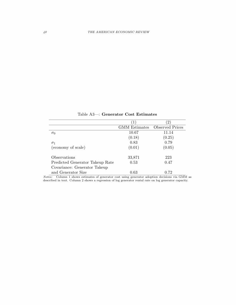
We parametrize the generator cost as lnCGit = �0 + �1 ln(cit), where �1 is the

economy of scale parameter, and cit is the generator capacity in kilowatts. Weestimate �0 and �1 using GMM, matching the mean generator adoption rate andthe covariance between generator adoption and log generator capacity. We usethe identity matrix as a weighting matrix, since the two moments that we matchare of comparable scales. Column 1 of Table A3 presents GMM estimates of thegenerator cost function.For comparison, we collected generator purchase price data from the United

States. To compare to the estimated CG , we must first convert the purchaseprices into yearly rental prices. First, we convert generators rated in KVA intoKW using a 0.8 conversion ratio. Second, we convert US dollars into Rupees usinga 50 to 1 exchange rate. Finally, we convert the purchase price of a generatorinto an annual rental price assuming a 30 percent discount rate, a ten percentdepreciation rate, and a ten-year generator lifespan.7 This gives a 1.6:1 ratiobetween generator costs and rental rates. Column 2 presents a regression of thenatural logs of these observed prices on natural log of capacity.The estimates of �1 are close to 0.8 in both columns of Table A3. The estimates

of �0 are also comparable (10.67 vs. 11.14), although the point estimate in column1 is smaller. This gives us some confidence that the estimated generator costsare approximately reasonable and that generator costs can explain the fact thatmany manufacturing plants in the ASI do not have generators.

7This 30 percent discount rate is high by U.S. standards, but as Banerjee and Duflo (2014) discuss,Indian firms pay far higher interest rates - on the order of 30 to 60 percent, if they have access to capitalat all.


Table A3—: Generator Cost Estimates

(1) (2)GMM Estimates Observed Prices

�0 10.67 11.14(0.18) (0.25)

�1 0.83 0.79(economy of scale) (0.01) (0.05)

Observations 33,871 223Predicted Generator Takeup Rate 0.53 0.47Covariance: Generator Takeupand Generator Size 0.63 0.72

Notes: Column 1 shows estimates of generator cost using generator adoption decisions via GMM asdescribed in text. Column 2 shows a regression of log generator rental rate on log generator capacity.


F7. Additional Simulation Figures and Tables

Figure A1. : Predicted Average Revenue Loss by Simulation Year

0

2

4

6

8

10

Perc

ent R

even

ue L

oss

1990 1995 2000 2005 2010year

Notes: In the body of the paper, we simulate e↵ects of moving from � = 0 to � = Ss2005 for all plantsin the data in 2005. This figure presents revenue e↵ects from the same simulations for each year of the1992-2010 sample, i.e. taking the sample of plants in year t and changing � from � = 0 to � = Sst.


Figure A2. : Generator Adoption Under Varying Shortage Levels

0

.2

.4

.6

.8

1

Gen

erat

or U

ptak

e

0 .05 .1 .15 .2Shortage

Notes: These figures show the simulated generator adoption rate when the � on the x-axis is assigned toall plants in the 2005 ASI, using the generator adoption model in Section VI.VI.A. Note that generatortakeup exceeds 90 percent at a seven percent �, which may seem puzzling given that the generator costestimates are based on a 44 percent takeup rate in the ASI at a 7.2 percent mean shortage. The reasonis that the distribution of Ss2005 across plants is right skewed; the median of Ss2005 across plants is only3.5 percent.


Table A4—: E↵ect of Shortages: Semi-elasticities from Model and IVEstimates

(1) (2) (3)p-Value

IV for ColumnsSimulation Estimate (1) vs. (2)

Self-Generation Share Increase 0.29% 0.44% (0.33)Materials Reduction 0.91% 1.14% (0.66)Labor Reduction 0.91% 0.24% (0.05)Revenue Loss 0.91% 1.09% (0.74)TFPR Loss 0.19% 0.30% (0.66)

Notes: This table parallels columns 1 and 2 of Panel A of Table 9, except that it presents semi-elasticities, i.e. the e↵ect of a one percentage point increase in shortages on percent changes in thedependent variable.


Table A5—: Counterfactuals Under Varying Shortage Levels

(1) (2) (3) (4) (5)Shortage Percent (�): 3% 5% 7% 10% 20%Exogenous GeneratorsRevenue Loss: Average 2.5% 4.2% 5.8% 8.3% 16%Revenue Loss: Generators 0.2% 0.3% 0.5% 0.6% 1.3%Revenue Loss: Non-Generators 4.5% 7.4% 10% 15% 28%

TFPR Loss: Average 0.5% 0.9% 1.3% 1.9% 3.9%

Input Cost Increase: Generators 0.2% 0.3% 0.4% 0.5% 1.0%

Variable Profit Loss: Average 2.5% 4.2% 5.8% 8.2% 16%Generator Cost (Percent of Profits) 3.0% 3.0% 3.0% 3.1% 3.2%Total Profit Loss: Average 5.5% 7.2% 8.8% 12% 19%

Endogenous GeneratorsGenerator Take-up 66% 85% 91% 94% 98%

Revenue Loss: Average 1.7% 1.4% 1.3% 1.3% 1.7%Revenue Loss: Generators 0.2% 0.3% 0.4% 0.6% 1.2%Revenue Loss: Non-Generators 4.2% 7.1% 10% 15% 29%

TFPR Loss: Average 0.4% 0.2% 0.2% 0.2% 0.1%

Input Cost Increase: Generators 0.1% 0.2% 0.3% 0.5% 1.0%

Variable Profit Loss: Average 1.7% 1.4% 1.2% 1.2% 1.5%Generator Cost (Percent of Profits) 1.6% 2.7% 3.4% 3.8% 4.6%Total Profit Loss: Average 3.3% 4.1% 4.6% 5.1% 6.1%

Notes: This table presents predictions of the simulation model described in the text. The simulationswith “exogenous” generators hold fixed the generator adoption decision observed in the ASI, whilethe simulations with “endogenous” generators use the model’s prediction of which plants will purchasegenerators at the di↵erent shortage levels. Input Cost Increase is reported as a share of revenues. In thistable, the electricity shortage is uniform across all plants in all states.


*

REFERENCES

Banerjee, Abhijit and Esther Duflo (2014). “Do Firms Want to Borrow More?Testing Credit Constraints Using a Directed Lending Program.” Review of Eco-nomic Studies, Vol. 81, pp. 572–607.

MOSPI (Ministry of Statistics and Programme Implemen-tation (2014). “Annual Survey of Industries.” Available at:http://mospi.nic.in/Mospi New/upload/asi/ASI main.htm?status=1&menu id=88.Accessed 17 December 2014.

Documents

Online Appendix for “How Do Electricity Shortages A … Appendix for “How Do Electricity Shortages A↵ect Industry? Evidence from India ... Anuradha Bhatta,