Online Prediction under Model Uncertainty ViaDynamic Model Averaging: Application to a Cold

Rolling Mill ∗

Adrian E. RafteryUniversity of Washington

Seattle, USA

Miroslav KarnyAcademy of Sciences

Czech Republic

Pavel EttlerCOMPUREG Plzen, s.r.o.

Plzen, Czech Republic

May 14, 2008; Revised July 3, 2009

Abstract

We consider the problem of online prediction when it is uncertain what the bestprediction model to use is. We develop a method called Dynamic Model Averaging(DMA) in which a state space model for the parameters of each model is combinedwith a Markov chain model for the correct model. This allows the “correct” modelto vary over time. The state space and Markov chain models are both specified interms of forgetting, leading to a highly parsimonious representation. As a special case,when the model and parameters do not change, DMA is a recursive implementation ofstandard Bayesian model averaging, which we call recursive model averaging (RMA).The method is applied to the problem of predicting the output strip thickness fora cold rolling mill, where the output is measured with a time delay. We found thatwhen only a small number of physically motivated models were considered and one wasclearly best, the method quickly converged to the best model, and the cost of modeluncertainty was small; indeed DMA performed slightly better than the best physical

∗Adrian E. Raftery is Blumstein-Jordan Professor of Statistics and Sociology, Box 354322, Universityof Washington, Seattle, WA 98195-4322; email: raftery@u.washington.edu. Miroslav Karny is Head De-partment of Adaptive Systems, Institute of Information Theory and Automation (UTIA), Czech Academyof Sciences, Prague, Czech Republic; email: school@utia.cas.cz. Pavel Ettler is with COMPUREG Plzen,s.r.o., 30634 Plzen, Czech Republic; email: ettler@compureg.cz. Raftery’s research was supported by Na-tional Science Foundation Grant No. ATM 0724721, the Joint Ensemble Forecasting System (JEFS) undersubcontract No. S06-47225 from the University Corporation for Atmospheric Research (UCAR), and theDoD Multidisciplinary Research Initiative (MURI) administered by the Office of Naval Research undergrant N00014-01-10745. Karny’s was supported by grant number 1ET 100 750 401 from the Academy ofSciences of the Czech Republic, “Bayesian adaptive distributed decision making,” and by grant number1M0572 from the Czech Ministry of Education, Youth and Sports (MSMT), “Research Center DAR.” Theauthors are grateful to Josef Andrysek for helpful research assistance, and to the editor, the associate editorand two anonymous referees for very helpful comments that improved the manuscript. Part of this researchwas carried out while Raftery was visiting UTIA.

i

model. When model uncertainty and the number of models considered were large, ourmethod ensured that the penalty for model uncertainty was small. At the beginning ofthe process, when control is most difficult, we found that DMA over a large model spaceled to better predictions than the single best performing physically motivated model.We also applied the method to several simulated examples, and found that it recoveredboth constant and time-varying regression parameters and model specifications quitewell.

1 Introduction

We consider the problem of online prediction when it is uncertain what the best prediction

model to use is. Online prediction is often done for control purposes and typically uses a

physically-based model of the system. Often, however, there are several possible models and

it is not clear which is the best one to use.

To address this problem, we develop a new method called Dynamic Model Averaging

(DMA) that incorporates model uncertainty in a dynamic way. This combines a state space

model for the parameters of each of the candidate models of the system with a Markov

chain model for the best model. Both the state space and Markov chain models are esti-

mated recursively, allowing which model is best to change over time. Both the state space

and Markov chain models are specified using versions of forgetting, which allows a highly

parsimonious representation. The predictive distribution of future system outputs is a mix-

ture distribution with one component for each physical model considered, and so the best

prediction is a weighted average of the best predictions from the different models.

The physical theory underlying the prediction or control problem is often somewhat

weak, and may be limited essentially to knowing what the inputs are that could potentially

influence the output of a system. In that case we consider a model space consisting of all

possible combinations of inputs that are not excluded by physical considerations.

The DMA methodology combines various existing ideas, notably Bayesian model av-

eraging, hidden Markov models, and forgetting in state space modeling. Bayesian model

averaging (BMA) (Leamer 1978; Raftery 1988; Hoeting et al. 1999; Clyde and George 2004)

is an established methodology for statistical inference from static datasets in the presence

of model uncertainty, and has been particularly well developed for linear regression when

there is uncertainty about which variables to include (Raftery, Madigan, and Hoeting 1997;

Fernandez, Ley, and Steel 2001; Eicher, Papageorgiou, and Raftery 2009). BMA usually ad-

dresses the problem of uncertainty about variable selection in regression by averaging over all

possible combinations of regressors that are not excluded by physical considerations. BMA

is restricted to static problems, however. An extension to dynamic updating problems was

proposed by Raftery et al. (2005) in the context of probabilistic weather forecasting, using

a sliding window estimation period consisting of a specified previous number of days. DMA

is a recursive updating method rather than a windowing one.

1

The idea of the hidden Markov model is that there is an underlying unobserved discrete-

valued process whose value affects the system state and which evolves according to a Markov

chain. The idea seems first to have been proposed independently by Ackerson and Fu (1970)

for the case where the noise in a Kalman filter is a Gaussian mixture, and by Harrison and

Stevens (1971) for modeling time series that can have outliers and jumps in level and trend.

The latter has been extended to the dynamic linear model (Harrison and Stevens 1976;

West and Harrison 1989) and the multiprocess Kalman filter (Smith and West 1983). The

basic idea has since been widely used, often under different names, in different disciplines

including speech recognition (Rabiner 1989) and genomics (Eddy 1998, 2004). In economics,

the Markov switching model of Hamilton (1989) is widely used for time series in which the

autoregressive parameters switch between different regimes. Markov switching models are

also widely used for tracking moving or manoeuvering objects, particularly in aerospace en-

gineering (Li and Jilkov 2005). An important unifying framework is the conditional dynamic

linear model (CDLM) of Chen and Liu (2000), which includes several earlier proposals as

special cases,

To specify DMA, we postulate the existence of a hidden Markov chain on the model

space. This differs from many other hidden Markov applications because the definition of

the state itself, and not just its value, depends on the current value of the chain. As a result,

our method is not a special case of the CDLM, although it is related to it.

One of the difficulties with hidden Markov models is the need to make inference about the

full sequence of hidden values of the chain, and the resulting computational explosion. Vari-

ous approximations have been proposed, including finite-memory approximations (Ackerson

and Fu 1970; West and Harrison 1989), the interacting multiple model (IMM) algorithm of

Blom and Bar-Shalom (1988), which is popular in tracking applications (Mazor et al. 1998),

the particle filter (Gordon, Salmond, and Smith 1993), also known as sequential importance

sampling, and the ensemble Kalman filter (Evensen 1994). The fact that in our case the

state vector has a different definition for each candidate model allows us to use a very simple

approximation in which each model is updated individually at each time point. We show that

this is equivalent to an age-weighted version of BMA, which makes it intuitively appealing

in its own right.

As a special case, when the model and parameters do not change, DMA is a recursive im-

plementation of standard Bayesian model averaging, which we call recursive model averaging

(RMA).

In many previous hidden Markov applications there is considerable information about

the evolution of the state. In the rolling mill application that motivated our work, there is

considerable physical knowledge about the rolling mill itself, but little physical knowledge

about how the regression model and its parameters (which define the system state in our

setup) are likely to evolve. All that can be assumed is that the parameters are likely to

2

evolve gradually in time, and that the model is likely to change infrequently. As a result,

rather than specify the state space model fully, which is demanding and for which adequate

information is not available, we specify the evolution of the parameters and the model by

exponential forgetting (Fagin 1964; Jazwinsky 1970; Kulhavy and Zarrop 1993).

We illustrate the methodology by applying it to the prediction of the outgoing strip

thickness of a cold rolling mill, ultimately for the purpose of either human or automatic

control. The system input and three adjustable control parameters are measured, and the

system output is measured with a time delay. While there is considerable understanding of

the physics of the rolling mill, three plausible models have been proposed, of which two are

physically motivated. We first implemented DMA for these three models, one of which turned

out to be clearly best. DMA converged rapidly to the best model, and the performance of

DMA was almost the same as that of the best model — DMA allowed us to avoid paying a

penalty for being uncertain about model structure.

We then extended the set of models to allow for the possibility of each of the inputs

having an effect or not, yielding a much bigger model space with 17 models. In this case we

found that DMA performed better than the best physical model in the initial, most unstable

period when control is most difficult, and comparably over the rest of the period, when

prediction errors were generally stable. Thus, even in this case with a larger model space,

DMA allowed us to avoid paying a penalty for model uncertainty, and indeed allowed us to

use the model uncertainty to increase the stability of the predictions in the early unstable

period.

To assess how well the method recovered time-varying and constant regression parameter

values and model specifications, we also applied it to four simulated examples closely modeled

on the rolling mill problem.

The rest of the paper is organized as follows. In Section 2 we describe the rolling mill

problem that motivated our research. In Section 3 we describe the dynamic model averaging

methodology, and in Section 4 we show the results of single-model and DMA prediction for

the rolling mill. In Section 5 we give the results of applying our method to four simulated

examples. In Section 6 we discuss limitations, possible extensions and alternatives to the

proposed methodology.

2 The Rolling Mill Problem

The problem that motivated our methodology is that of predicting the output of a reversing

cold rolling mill. A cold rolling mill is a machine used for reducing the thickness of metal

strips; a schematic drawing is shown in Figure 1. Metal is passed through a gap and subjected

to the rolling force. The strip thickness is measured by diamond-tipped contact meters on

both sides of the rolling mill, providing measurements of the input and output thickness. A

3

Thickness meter

Rolling force

Thickness meter

Direction of rolling

Roll position

Figure 1: Schematic drawing of a reversing cold rolling mill.

target thickness is defined, and this needs to be achieved with high accuracy depending on

the nominal thickness. In our case a typical tolerance was ± 10 microns. We are dealing here

with a reversing rolling mill which reduces the strip thickness in several passes, alternating

the rolling direction.

The output that we want to predict is the output strip thickness which is, under normal

conditions, securely controlled using automatic gauge control (Ettler and Jirovsky 1991).

This control method can be improved manually by actions of the operators, potentially

supported by a decision-support system (Quinn et al. 2003; Ettler, Karny, and Guy 2005).

Reliable thickness prediction can improve control, particularly under adverse conditions

that the automatic gauge control system is not designed to handle. These can arise at the

beginning of a pass of the material through the rolling mill, when the thickness meters often

do not operate for a period because there is a danger that they may be damaged. Adverse

conditions can also arise for welded strips and for strip parts with uneven surfaces.

Important variables that can be adjusted to achieve the target are the size of the rolling

gap governed by the roll positioning system, the rolling force, the input and output rolling

speeds and – possibly – strip tensions. Rolling forces can be of the order of 106 N, and rolling

speeds of the order of 0.1–8 m/s. The rolling gap cannot be reliably measured, but the roll

position is available instead, measured against the mill frame. This position differs from the

gap mainly because of frame elongation during rolling.

Modern rolling mill control systems allow every sample processed to be archived. Data

collection is triggered by the strip movement. In our case, data samples are recorded every

4 cm, so that the sampling period varies according to the strip speed. For instance, if the

speed is 1 m/s, the sampling period is 40 milliseconds. This imposes constraints on the

complexities of online data processing, which must be completed well within the sampling

4

L

D

Figure 2: Measurement Time Delay. A measurement is made every time the material movesby a length ∆, equal to one sample. The output thickness currently at the gap is notmeasured until the material has moved a distance L beyond the gap. The measurement timedelay is d ≈ L/∆ samples, where d is a natural number.

period. These constraints are a key element of the problem, and imply that the methods

used must be computationally efficient.

Our goal is to predict the output thickness for the piece of the strip just leaving the rolling

gap. We wish to do this online, either to provide guidance to human operators controlling

the system in real time in situations that preclude the use of automatic gauge control, or as

an additional input to the control system. This is essentially a regression problem. However,

an important complicating aspect of the data collection system is the time delay problem,

illustrated in Figure 2.

Current values of the regressors are available for the piece of the strip in the rolling

gap. However, the system output — the output strip thickness — is measured only with

a delay d, which in our case was d = 24 samples. The task thus consists of predicting the

output thickness, given the input thickness and other measured data at the gap. But data

for estimating the regression relationship are available only with a delay d.

The data that we analyze come from a strip of length about 750 m that yielded 19058

samples. The roll position was controlled by automatic gauge control with feedback. The

data from the first 1000 samples are shown in Figure 3. Figure 3(a) shows the deviations

of the input and output thicknesses from their nominal values, which are 1398 and 1180

microns, respectively. (The input was about 200 microns thicker than the desired output,

allowing a margin for the rolling mill to do its work of thinning the material.) Initially the

output was too thick, and gradually converged to a relatively stable situation after about 600

samples. Figure 3(b) shows the roll position, Figure 3(c) the ratio of the input to the output

rolling speeds, and Figure 3(d) the rolling force. The gradual adjustment of the controlled

variable by the feedback controller can be seen. The two outliers in the rolling speed ratio

at samples 42 and 43 provide a challenge to the system.

5

0 200 400 600 800 1000

-40

-20

020

4060

Sample

Inpu

t and

out

put t

hick

ness

: Dev

iatio

ns fr

om ta

rget

Input thicknessOutput thickness

0 200 400 600 800 1000

100

150

200

250

Sample

Rol

l pos

ition

(m

icro

ns)

(a) Input and output thickness (b) Roll positiondeviations from target

0 200 400 600 800 1000

0.65

0.70

0.75

0.80

0.85

0.90

0.95

Sample

Rat

io o

f rol

ling

spee

ds

0 200 400 600 800 1000

2.1

2.2

2.3

2.4

2.5

Sample

Rol

ling

forc

e (M

N)

(c) Ratio of rolling speeds (d) Rolling force

Figure 3: Data from the rolling mill: first 1000 samples. (a) Input and output thicknessdeviations from their nominal values (in microns); (b) Roll position (in microns); (c) Ratioof input to output rolling speeds; (d) Rolling force at the gap (in MN).

6

3 Dynamic Model Averaging (DMA)

We first consider the situation where a single, physically-based regression-type model is

available for prediction. We will review a standard state-space model with forgetting for

adaptive estimation of the regression parameters and prediction with time delay. This is

essentially standard Kalman filtering, but we review it here to fix ideas and notation. We will

then address the situation where there is uncertainty about the model structure and several

plausible models are available. For concreteness, we will use the rolling mill terminology.

3.1 The One-Model Case

Let yt be the deviation of the output thickness of sample t from its target value, and let xt =

(xtj : j = 1, . . . , ν) be the corresponding vector of inputs. Typically xt1 = 1, corresponding

to the regression intercept, and xt will also include the input thickness and other inputs and

possibly also a past value of the output; the latter would lead to an ARX model (Ljung

1987).

The observation equation is then

yt = xTt θt + εt, (1)

where a superscript T denotes matrix transpose, θt is a vector of regression parameters

and the innovations εt are distributed as εtiid∼ N(0, V ), where N(µ, σ2) denotes the normal

distribution with mean µ and variance σ2. The regression parameters θt are allowed to evolve

according to the state equation

θt = θt−1 + δt, (2)

where the state innovations δt are distributed as δtind∼ N(0,Wt).

Inference is done recursively using Kalman filter updating. Suppose that θt−1|Y t−1 ∼N(θt−1,Σt−1), where Y t−1 = {y1, . . . , yt−1}. Then

θt|Y t−1 ∼ N(θt−1, Rt), (3)

where

Rt = Σt−1 +Wt. (4)

Equation (3) is called the prediction equation.

Specifying the ν× ν matrix Wt completely is demanding, and often little information for

doing so is available. Instead we follow Fagin (1964) and Jazwinsky (1970) and specify it

using a form of forgetting. This consists of replacing (4) by

Rt = λ−1Σt−1, (5)

where λ is called the forgetting factor and is typically slightly below 1. The resulting model

is a properly defined state space model, with Wt = aΣt−1, where a = (λ−1 − 1). As pointed

7

out, for example, by Hannan, McDougall, and Poskitt (1989), estimation in this model is

essentially age-weighted estimation where data i time points old has weight λi, and the

effective amount of data used for estimation, or the effective window size, is h = 1/(1− λ).

This suggests that forgetting may be roughly comparable to windowing (Jazwinsky 1970),

in which the last h available samples are used for estimation and are equally weighted. A

windowing method like this was used in the multimodel context by Raftery et al. (2005).

Inference is completed by the updating equation,

θt|Y t ∼ N(θt,Σt). (6)

In (6),

θt = θt−1 +RtxTt (V + xTt Rtxt)

T et, (7)

where et = yt − xTt θt−1 is the one-step-ahead prediction error, and

Σt = Rt −Rtxt(V + xTt Rtxt)−1xTt Rt. (8)

The inference process is repeated recursively as the measurements on a new sample become

available. It is initialized by specifying θ0 and Σ0; we will discuss their values for the rolling

mill problem in Section 4.

The information available for predicting yt is d samples old because of the time-delay

problem, and so we use

yt = xTt θt−d−1. (9)

The observations innovations variance V needs to be specified by the user. Here we

estimate it by a recursive method of moments estimator, using the fact that the one-step-

ahead predictive distribution of yt is given by

yt|Y t−1 ∼ N(xTt θt−1, V + xTt Rtxt). (10)

It follows that

V ∗t =1

t

t∑r=1

[(yt − xtθt−1)2 − xTt Rtxt]

is a consistent estimator of V in the sense that V ∗t −→ V as t −→ ∞ in probability under

the model defined by (1) and (2). It is not guaranteed, however, that V ∗t > 0. This leads us

to define the recursive moment estimator

Vt =

{At if At > 0;

Vt−1 otherwise,

where

At =

(t− 1

t

)Vt−1 +

1

t(e2t − xTt Rtxt).

8

3.2 The Multi-Model Case

We now consider the case where multiple models, M1, . . . ,MK are considered and there is

uncertainty about which one is best. We assume that each model can be expressed in the

form of equations (1) and (2), where the state and predictor vectors for each model are

different. They can be of different dimensions and need not overlap. The quantities specific

to model Mk are denoted by a superscript (k). We let Lt = k if the process is governed by

model Mk at time t. We rewrite (1) and (2) for the multimodel case as follows:

yt|Lt = k ∼ N(x(k)Tt θ

(k)t , V (k)), (11)

θ(k)t |Lt = k ∼ N(θ

(k)t−1,W

(k)t ). (12)

We assume that the model governing the system changes infrequently, and that its evolu-

tion is determined by a K ×K transition matrix Q = (qk`), where qk` = P [Lt = `|Lt−1 = k].

The transition matrix Q has to be specified by the user, which can be onerous when the

number of models is large. Instead we again avoid this problem by specifying the transition

matrix implicitly using forgetting.

Estimation of θ(k)t in general involves a mixture of Kt terms, one for each possible value

of Lt = {L1, . . . , Lt}, as described by Ackerson and Fu (1970) and Chen and Liu (2000),

for example. This number of terms rapidly becomes enormous, making direct evaluation

infeasible, and many different approximations have been described in the literature. Here

we are interested in prediction of the system output, yt, given Y t−1, and this depends on θ(k)t

only conditionally on Lt = k. This leads to a simple approximation that works well in this

case, consisting of simply updating θ(k)t conditionally on Lt = k for each sample.

In this multimodel setup, the underlying state consists of the pair, (θt, Lt), where θt =

(θ(1)t , . . . , θ

(K)t ). The quantity θ

(k)t is defined only when Lt = k, and so the probability

distribution of (θt, Lt) can be written

p(θt, Lt) =K∑k=1

p(θ

(k)t |Lt = k

)p(Lt = k). (13)

The distribution in (13) is what we will update as new data become available.

Estimation thus proceeds analogously to the one-model case, consisting of a prediction

step and an updating step. Suppose that we know the conditional distribution of the state

at time (t− 1) given the data up to that time, namely

p(θt−1, Lt−1|Y t−1) =K∑k=1

p(θ

(k)t−1|Lt−1 = k, Y t−1

)p(Lt−1 = k|Y t−1), (14)

where the conditional distribution of θ(k)t−1 is approximated by a normal distribution, so that

θ(k)t−1|Lt−1 = k, Y t−1 ∼ N(θ

(k)t−1,Σ

(k)t−1). (15)

9

The prediction step then involves two parts: prediction of the model indicator, Lt, via

the model prediction equation, and conditional prediction of the parameter, θ(k)t , given that

Lt = k, via the parameter prediction equation. We first consider prediction of the model

indicator, Lt. Let πt−1|t−1,` = P [Lt−1 = `|Y t−1]. Then the model prediction equation is

πt|t−1,k ≡ P [Lt = k|Y t−1]

=K∑`=1

πt−1|t−1,` qk`. (16)

To avoid having to explicitly specify the transition matrix, with its K2 elements, we replace

(16) by

πt|t−1,k =παt−1|t−1,k + c∑K`=1 π

αt−1|t−1,` + c

. (17)

In (17), α is a forgetting factor, which will typically be slightly less than 1, and c is a small

positive number, introduced to avoid a model probability being brought to machine zero by

aberrant observations; we set this to c = .001/K. Equation (17) increases the uncertainty by

flattening the distribution of Lt. This is a slight generalization of the multiparameter power

steady model introduced independently by Peterka (1981) and Smith (1981), generalizing

the one-dimensional steady model of Smith (1979). Although the resulting model does not

specify the transition matrix of the Markov chain explicitly, Smith and Miller (1986) argued

that this is not a defect of the model, since the data provide information about πt−1|t−1,k and

πt|t−1,k, but no additional information about Q. Exponential forgetting has been used for

updating discrete probabilities in a different two-hypothesis context by Karny and Andrysek

(2009).

With forgetting, the parameter prediction equation is

θ(k)t |Lt = k, Y t−1 ∼ N(θ

(kt−1, R

(k)t ), (18)

where R(k)t = λ−1Σ

(k)t−1.

We now consider the updating step, which again has two parts, model updating and

parameter updating. The model updating equation is

πt|t,k = ωtk/

K∑`=1

ωt`, (19)

where

ωt` = πt|t−1,` f`(yt|Y t−1). (20)

In (20), f`(yt|Y t−1) is the density of a N(x(`)Tt θ

(`)t−1, V

(`)+x(`)Tt R

(`)t x

(`)t ) distribution, evaluated

at yt.

The parameter updating equation is

θ(k)|Lt = k, Y t ∼ N(θ(k)t ,Σ

(k)t ), (21)

10

where θ(k)t is given by (7) and Σ

(k)t is given by (8), in each case with the superscript (k) added

to all quantities. This process is then iterated as each new sample becomes available. It is

initialized by setting π0|0,` = 1/K for ` = 1, . . . , K, and assigning values to θ(k)0 and Σ

(k)0 .

The model-averaged one-step-ahead prediction of the system output, yt, is then

yDMAt =

K∑k=1

πt|t−1,k y(k)t

=K∑k=1

πt|t−1,k x(k)Tt θ

(k)t−1. (22)

Thus the multimodel prediction of yt is a weighted average of the model-specific predictions

y(k)t , where the weights are equal to the posterior predictive model probabilities for sample t,

πt|t−1,k. For the rolling mill problem with delayed prediction, we take the predicted value of

yt to be

yDMAt =

K∑k=1

πt−d|t−d−1,k y(k)t

=K∑k=1

πt−d|t−d−1,k x(k)Tt θ

(k)t−d−1. (23)

One could also project the model probabilities into the future and allow for model transitions

during the delay period by replacing πt−d|t−d−1,k in (23) by παd

t−d|t−d−1,k, but we do not do

this here.

We call the method dynamic model averaging (DMA), by analogy with Bayesian model

averaging for the static linear regression model (Raftery, Madigan, and Hoeting 1997).

3.3 Connection to Static Bayesian Model Averaging

Standard Bayesian model averaging (BMA) addresses the static situation where the correct

model Mk and its parameter θ(k) are taken to be fixed but unknown. In that situation, the

BMA predictive distribution of yn+d given Y n is

p(yn+d|Y n) =K∑k=1

p(yn+d|Y n,Mk)p(Mk|Y n).

where p(Mk|Y n) is the posterior model probability of Mk. If, as here, all models have equal

prior probabilities, this is given by

p(Mk|Y n) =p(Y n|Mk)∑K`=1 p(Y

n|M`),

where p(Y n|Mk) =∫p(Y n|θ(k),Mk)p(θ

(k)|Mk)dθ(k) is the integrated likelihood, obtained by

integrating the product of the likelihood, p(Y n|θ(k),Mk), and the prior, p(θ(k)|Mk), over the

11

parameter space. See Hoeting et al. (1999) and Clyde and George (2004) for reviews of

BMA.

Dawid (1984) pointed out that the integrated likelihood can also be written as follows:

p(Y n|Mk) =n∏t=1

p(yt|Y t−1,Mk), (24)

with Y 0 defined as the null set. The posterior model probabilities in BMA can be expressed

using Bayes factors for pairwise comparisons. The Bayes factor for Mk against M` is defined

as the ratio of integrated likelihoods, Bk` = p(Y n|Mk)/p(Yn|M`) (Kass and Raftery 1995).

It follows from (24) that the log Bayes factor can be decomposed as

logBk` =n∑t=1

logBk`,t, (25)

where Bk`,t = p(yt|Y t−1,Mk)/p(yt|Y t−1,M`) is the sample-specific Bayes factor for sample t.

In the dynamic setup considered in the rest of the paper, it follows from (17), (19) and

(20) that when c = 0 in (17),

log

(πn|n,kπn|n,`

)=

n∑t=1

αn−t logBk`,t, (26)

where Bk`,t is defined as in (25). Thus our setup leads to the ratio of posterior model

probabilities at time n being equal to an exponentially age-weighted sum of sample-specific

Bayes factors, which is intuitively appealing.

When α = λ = 1 there is no forgetting and we recover the solution for the static situation

as a special case of DMA, as (25) and (26) are then equivalent. In this case, the method is

recursive but not dynamic, and could be called recursive model averaging (RMA). This may

have computational advantages over the standard computational methods for BMA. To our

knowledge this also is new in the literature.

4 Results for the Rolling Mill

For the rolling mill problem, the four candidate predictor variables of the deviation of the

output thickness from its target value for sample t, yt, are:

ut: the deviation of the input thickness from its nominal value for sample t,

vt: the roll position (in microns),

wt: the ratio of the output rolling speed to the input rolling speed, and

zt: the rolling force applied to sample t.

In previous work, three models have been used, the first two of which are physically

motivated (Ettler, Karny, and Nedoma 2007). The third model was based on exploratory

empirical work. All three have the regression form (1).

12

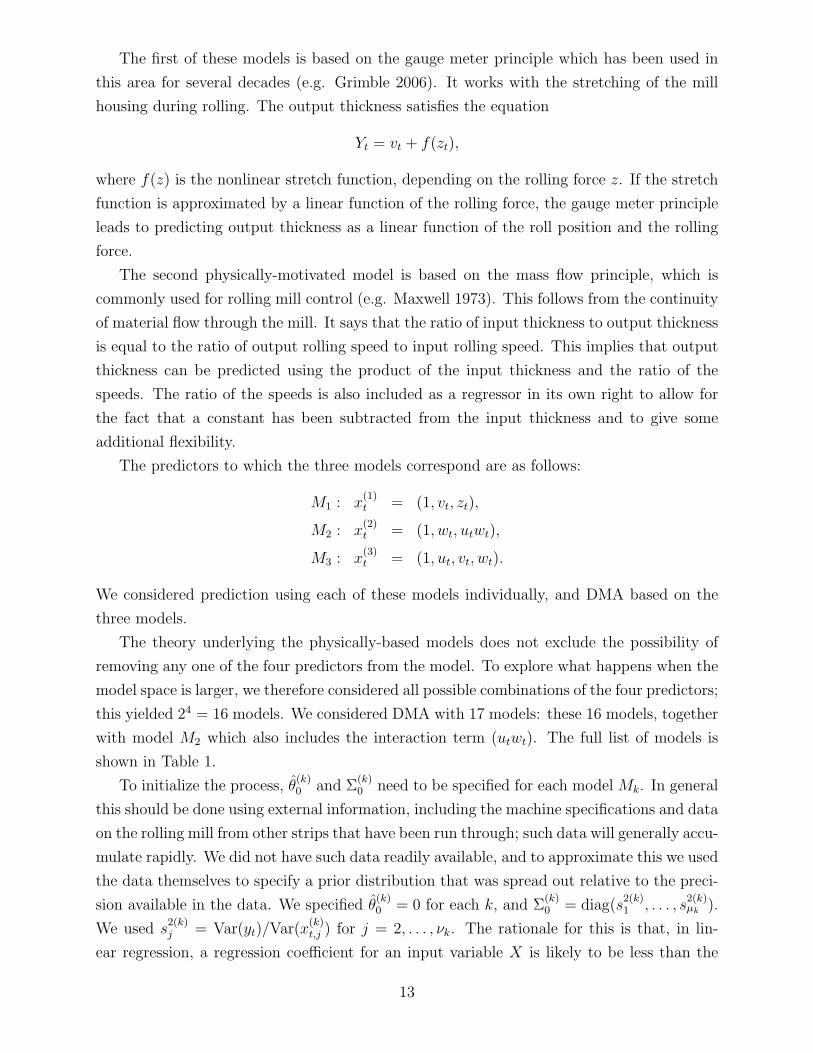
The first of these models is based on the gauge meter principle which has been used in

this area for several decades (e.g. Grimble 2006). It works with the stretching of the mill

housing during rolling. The output thickness satisfies the equation

Yt = vt + f(zt),

where f(z) is the nonlinear stretch function, depending on the rolling force z. If the stretch

function is approximated by a linear function of the rolling force, the gauge meter principle

leads to predicting output thickness as a linear function of the roll position and the rolling

force.

The second physically-motivated model is based on the mass flow principle, which is

commonly used for rolling mill control (e.g. Maxwell 1973). This follows from the continuity

of material flow through the mill. It says that the ratio of input thickness to output thickness

is equal to the ratio of output rolling speed to input rolling speed. This implies that output

thickness can be predicted using the product of the input thickness and the ratio of the

speeds. The ratio of the speeds is also included as a regressor in its own right to allow for

the fact that a constant has been subtracted from the input thickness and to give some

additional flexibility.

The predictors to which the three models correspond are as follows:

M1 : x(1)t = (1, vt, zt),

M2 : x(2)t = (1, wt, utwt),

M3 : x(3)t = (1, ut, vt, wt).

We considered prediction using each of these models individually, and DMA based on the

three models.

The theory underlying the physically-based models does not exclude the possibility of

removing any one of the four predictors from the model. To explore what happens when the

model space is larger, we therefore considered all possible combinations of the four predictors;

this yielded 24 = 16 models. We considered DMA with 17 models: these 16 models, together

with model M2 which also includes the interaction term (utwt). The full list of models is

shown in Table 1.

To initialize the process, θ(k)0 and Σ

(k)0 need to be specified for each model Mk. In general

this should be done using external information, including the machine specifications and data

on the rolling mill from other strips that have been run through; such data will generally accu-

mulate rapidly. We did not have such data readily available, and to approximate this we used

the data themselves to specify a prior distribution that was spread out relative to the preci-

sion available in the data. We specified θ(k)0 = 0 for each k, and Σ

(k)0 = diag(s

2(k)1 , . . . , s

2(k)µk ).

We used s2(k)j = Var(yt)/Var(x

(k)t,j ) for j = 2, . . . , νk. The rationale for this is that, in lin-

ear regression, a regression coefficient for an input variable X is likely to be less than the

13

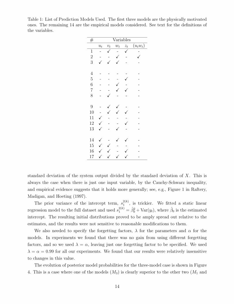
Table 1: List of Prediction Models Used. The first three models are the physically motivatedones. The remaining 14 are the empirical models considered. See text for the definitions ofthe variables.

# Variablesut vt wt zt (utwt)

1 - X - X -2 - - X - X3 X X X - -

4 - - - - -5 - - - X -6 - - X - -7 - - X X -8 - X - - -

9 - X X - -10 - X X X -11 X - - - -12 X - - X -13 X - X - -

14 X - X X -15 X X - - -16 X X - X -17 X X X X -

standard deviation of the system output divided by the standard deviation of X. This is

always the case when there is just one input variable, by the Cauchy-Schwarz inequality,

and empirical evidence suggests that it holds more generally; see, e.g., Figure 1 in Raftery,

Madigan, and Hoeting (1997).

The prior variance of the intercept term, s2(k)1 , is trickier. We fitted a static linear

regression model to the full dataset and used s2(k)1 = β2

0 + Var(yt), where β0 is the estimated

intercept. The resulting initial distributions proved to be amply spread out relative to the

estimates, and the results were not sensitive to reasonable modifications to them.

We also needed to specify the forgetting factors, λ for the parameters and α for the

models. In experiments we found that there was no gain from using different forgetting

factors, and so we used λ = α, leaving just one forgetting factor to be specified. We used

λ = α = 0.99 for all our experiments. We found that our results were relatively insensitive

to changes in this value.

The evolution of posterior model probabilities for the three-model case is shown in Figure

4. This is a case where one of the models (M3) is clearly superior to the other two (M1 and

14

0 50 100 150

0.0

0.2

0.4

0.6

0.8

1.0

Sample

Pos

terio

r Mod

el P

roba

bilit

y

Model 1Model 2Model 3

0 5000 10000 15000

0.0

0.2

0.4

0.6

0.8

1.0

Sample

Pos

terio

r Mod

el P

roba

bilit

y

(a) Samples 26–200 (b) All samples, 26–19058

Figure 4: Posterior Model Probabilities for the Three Initially Considered Models. Thecorrespondence between models and colors is the same in both plots.

M2). DMA quickly picks this up, and from Figure 4(a) we see that the posterior probability

of M3 rapidly grows close to 1 once enough data have been collected to allow a comparison.

However, this is not an absorbing state, and the other models occasionally become important,

as can be seen from the plot for all 19058 samples in Figure 4(b). Thus DMA is similar but

not identical to prediction based solely on M3 in this case.

The relative performance of the different methods is shown in Table 2. For all the

better methods, the prediction errors had stabilized by around sample 200. A key issue

for controlling the rolling mill is how quickly prediction stabilizes after the initial transient

situation. Thus we report performance results for the initial period, samples 26–200 (the first

25 samples cannot be predicted using the inputs because of the time delay of 24 samples),

and the remaining samples 201–19058. We report the mean squared value of the prediction

error, MSE, the maximum absolute prediction error, MaxAE, and the number of samples

for which the prediction error was greater than the desired tolerance of 10 microns.

Table 2 shows that M3 was much better than M1 or M2 for both periods, particularly

the initial period. For the initial period, DMA with 3 models was slightly better than M3 on

all three criteria we report, while for the stable period DMA was essentially the same as M3.

Thus DMA allows us to avoid paying a penalty for our uncertainty about model structure

in this case. Indeed, it even yields slightly more stable predictions in the initial unstable

period, perhaps because it allows some weight to be given to the simpler models, M1 and M2

at the very beginning, before enough data has accumulated to estimate the more complex

15

Table 2: Sample Statistics of Prediction Errors

Method Samples 26–200 Samples 201–19058MSE MaxAE #AE>10 MSE MaxAE #AE>10

Observed 2179.8 68.8 175 30.6 43.1 1183

Model 1 243.6 38.3 86 26.2 31.1 989Model 2 345.5 41.7 118 26.8 41.4 914Model 3 77.5 27.3 46 20.7 31.1 523

DMA – 3 models 76.1 26.3 45 20.7 31.1 520DMA – 17 models 68.9 22.0 42 20.6 31.1 519

NOTE: MaxAE is the maximum absolute error. “#AE>10” is the number of errors above 10microns in absolute value. The first line of the table refers to the deviations of the observedsystem output from the target value. Models 1, 2 and 3 are the three initially consideredmodels described in the text.

M3 accurately.

We now consider what happens when the space of candidate models is much larger, and 17

models are considered. Figure 5(a) shows the evolution of the posterior model probabilities

in the initial unstable period. Only four models (M3, M15, M16 and M17) have more than

negligible weight past the first 25 samples or so, and so, even with a large model space, DMA

yields a relatively parsimonious solution. In the initial unstable period, the relatively simple

model M15 had high weight, and in the later stable period, the more complex models M16

and M17 had more weight, as can be seen from Figure 5(b).

Table 2 shows, strikingly, that DMA with 17 models achieved significantly better per-

formance in the initial unstable period than either M3 or DMA with 3 models, on all three

criteria. This may be because it allows weight to be put on simple, parsimonious models

in the early period before stable data has accumulated to estimate more complex models

reliably. In the later stable period, DMA with 17 models did slightly better than both DMA

with 3 models, and than M3 on its own. Thus DMA yielded clear gains in the initial unstable

period and smaller ones in the later stable period. It allowed us to avoid paying a price for

model uncertainty, even when the model space was larger. Overall, including all possible

combinations of regressors led to better performance.

In order to investigate why DMA with 17 models did so well in the initial unstable

period, Figure 6(a) shows the prediction errors for M3 and DMA with 17 models. Figure

6(b) shows the absolute prediction error for DMA minus the absolute prediction error for M3

(so that positive values correspond to DMA doing better). Up to sample 50, there are large

positive values, and in samples 50–100 there are consistent nonnegligible positive values. In

samples 100–200 the differences are much smaller. This provides support for our conjecture:

16

0 50 100 150

0.0

0.2

0.4

0.6

0.8

Sample

Pos

terio

r Mod

el P

roba

bilit

y

Model 1Model 2Model 3Model 15Model 16Model 17All others

0 500 1000 1500 2000

0.0

0.2

0.4

0.6

0.8

Sample

Pos

terio

r Mod

el P

roba

bilit

y

(a) Samples 1–175 (b) Samples 1–2000

Figure 5: Posterior Model Probabilities for all 17 Models. The legends are the same in bothplots.

in essence, DMA does better in the initial unstable period because it is more adaptive than

a single model, even a good one such as M3, and being adaptive is more important during

the initial unstable period than later.

It is important for a real-time application such as this that methods run fast. Our

experiments were run in the interpreted statistical language R on a 2005 Apple Powerbook G4

laptop. Computer time scaled roughly linearly with the number of samples times the number

of models. DMA took about 2 milliseconds per model per sample. It seems reasonable to

expect that running it on newer hardware would speed it up by a factor of at least 4, and

that implementing the method in a more efficient, compiled language would speed it up by

a factor of 10 or more, suggesting speeds of about 0.05 milliseconds per model per sample

with good hardware and software in 2008. If one requires that computations take no more

than 20 milliseconds per sample, this suggests that with an efficient implementation, DMA

could be used for the rolling mill with up to about 400 models. It is thus well within the

range of practical application. Note that these time constraints preclude the use of methods

that are much more computer-intensive than the ones described here.

5 Simulated Examples

In the previous section, we assessed our method on the basis of its predictive performance

for the rolling mill data, which is what matters most for the application at hand. We now

17

50 100 150 200

-20

-10

010

20

Sample

Pre

dict

ion

erro

r

Model 3DMA

50 100 150 200

−2

02

46

8

Sample

Diff

eren

ce in

abs

olut

e pr

edic

tion

erro

rs

(a) Prediction errors for Model 3 and DMA (b) Difference in absolute prediction errors

Figure 6: Comparison of prediction errors for the best of the three initially considered modelsand for DMA: (a) Prediction errors for Model 3, and for DMA based on all 17 models. (b)Absolute prediction errors for Model 3 minus absolute prediction errors for DMA. Initialperiod, samples 26–200.

use four simulated examples, closely modeled on the rolling mill data, to assess the method’s

ability to recover the generating mechanism, including whether it favors the right model and

can track changing parameter values and model specifications.

In all four simulated examples, the length of the dataset (19058 samples) and the predictor

variables, ut, vt, wt and zt are the same as in the rolling mill example. Only the system

output, yt, is different.

In the first three simulated examples, the generating model remains constant over time.

It is Model 15, which includes ut and vt. However, the analyst does not know what the

generating model is, and so there is model uncertainty. In the first example, the regression

parameters also remain constant over time. In the second example, a regression parame-

ter changes smoothly over time, and in the third example a regression parameter changes

abruptly.

The first three simulation examples are as follows, where βut, βvt, βwt and βzt are the

regression parameters for ut, vt, wt and zt for sample t:

• Simulation 1 (constant parameters): βut = 0.35, βvt = 0.8, βwt = βzt = 0.

• Simulation 2 (smooth change in βut):

βut =

{0.5− 0.4t/12000 if t < 12000−0.2 + 0.4t/12000 otherwise,

18

βvt = 0.8, βwt = βzt = 0.

• Simulation 3 (abrupt change in βut at sample 12000): βut = 0.6 for t < 12000, βut = 0.2

for t ≥ 12000, βvt = 0.8, βwt = βzt = 0.

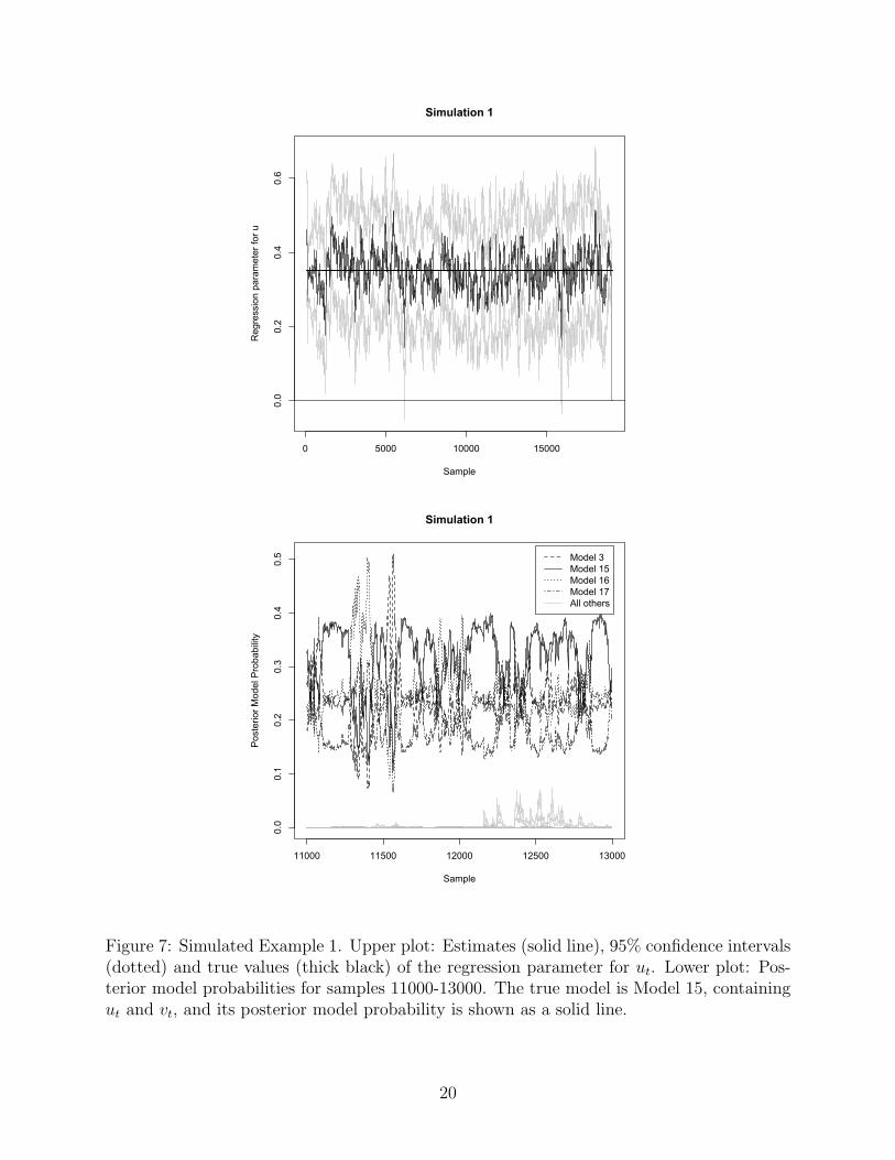
The results for the first simulated example are shown in Figure 7. The upper plot shows

estimates and confidence intervals for βut and the lower plot shows the posterior model

probabilities for samples 11000–13000. The estimates of βut remain close to the true value,

and the confidence interval contains the true value most (99.6%) of the time. The high

coverage of the confidence intervals reflects the fact that the model anticipates changes in

the regression parameter, and so is wider than needed to capture a constant parameter.

Model 15 is the true generating model, and its posterior model probability is shown by

the solid lines in the lower plot of Figure 7. It has the highest posterior probability among

all the 17 models most (73%) of the time. Models 3, 16 and 17 have nonnegligible posterior

probabilities much of the time also. Model 15 is nested within each of Models 3, 16 and 17,

and so they are also “correct,” in the sense that they include the generating mechanism as

a special case. The other 13 models are incorrect in that they do not include the generating

mechanism. The posterior model probabilities of the 13 incorrect models are all shown in

grey, and are small throughout.

For Simulation 2, the method tracks the value of the smoothly changing βut well, as

shown in Figure 8. For Simulation 3, the method adapts quickly to the abrupt change at

sample 12000 (Figure 9). In both these cases, the posterior model probabilities perform well,

similarly to Simulation 1.

Simulation 4 features a change of generating model at sample 12000, from Model 15

containing ut and vt, to Model 3, which also includes wt. Figure 10 shows the results. The

upper plot shows that the change in βwt from 0 to 50 at sample 12000 is well captured.

The lower plot shows the posterior model probabilities. Model 15 (solid) was the generating

model for the first 12000 samples, and it had the highest posterior probability for most

(69%) of these samples. Model 3 (dashed) was the generating model for the remaining 7058

samples, and it had the highest posterior probability for most (65%) of these samples.

Another way of looking at the posterior model probabilities is given by Figure 11. This

shows the log posterior odds for Model 3 (containing ut, vt and wt) against Model 15 (con-

taining just ut and vt). This can thus be viewed as showing a measure of the evidence for

an effect of wt; when it is positive it favors an effect, and when it is negative it favors no

effect. In the first 12000 samples, when there is no effect of wt, the posterior odds favor the

no-effect hypothesis 81% of the time, and in the remaining samples, when there is an effect

of wt, the posterior odds favor the hypothesis of an effect 79% of the time.

It is conventional to view Bayesian posterior odds as providing evidence “worth no more

than a bare mention” when they are between 1/3 and 3, namely when the log posterior odds

19

0 5000 10000 15000

0.0

0.2

0.4

0.6

Simulation 1

Sample

Reg

ress

ion

para

met

er fo

r u

11000 11500 12000 12500 13000

0.0

0.1

0.2

0.3

0.4

0.5

Simulation 1

Sample

Pos

terio

r Mod

el P

roba

bilit

y

Model 3Model 15Model 16Model 17All others

Figure 7: Simulated Example 1. Upper plot: Estimates (solid line), 95% confidence intervals(dotted) and true values (thick black) of the regression parameter for ut. Lower plot: Pos-terior model probabilities for samples 11000-13000. The true model is Model 15, containingut and vt, and its posterior model probability is shown as a solid line.

20

0 5000 10000 15000

0.0

0.2

0.4

0.6

0.8

Simulation 2

Sample

Reg

ress

ion

para

met

er fo

r u

11000 11500 12000 12500 13000

0.0

0.1

0.2

0.3

0.4

Simulation 2

Sample

Pos

terio

r Mod

el P

roba

bilit

y

Figure 8: Simulated Example 2. Upper plot: Estimates (solid line), 95% confidence intervals(dotted) and true values (thick black) of the regression parameter for ut. Lower plot: Pos-terior model probabilities for samples 11000-13000. The true model is Model 15, containingut and vt, and its posterior model probability is shown as a solid line. The legend is as inFigure 7.

21

0 5000 10000 15000

0.0

0.2

0.4

0.6

0.8

Simulation 3

Sample

Reg

ress

ion

para

met

er fo

r u

11000 11500 12000 12500 13000

0.0

0.1

0.2

0.3

0.4

0.5

Simulation 3

Sample

Pos

terio

r Mod

el P

roba

bilit

y

Figure 9: Simulated Example 3. Upper plot: Estimates (solid line), 95% confidence intervals(dotted) and true values (thick black) of the regression parameter for ut. Lower plot: Pos-terior model probabilities for samples 11000-13000. The true model is Model 15, containingut and vt, and its posterior model probability is shown as a solid line. The legend is as inFigure 7.

22

0 5000 10000 15000

-100

0100

200

Simulation 4

Sample

Reg

ress

ion

para

met

er fo

r w

11000 11500 12000 12500 13000

0.0

0.2

0.4

0.6

0.8

1.0

Simulation 4

Sample

Pos

terio

r Mod

el P

roba

bilit

y

Model 3Model 15Model 16Model 17All others

Figure 10: Simulated Example 4: Upper plot: Estimates (solid line), 95% confidence inter-vals (dotted), and true values (thick solid) of the regression parameter for ut. Lower plot:Posterior model probabilities for samples 11000-13000. The true model up to sample 12000is Model 15, containing ut and vt, shown as a solid line. After sample 12000, the true modelis Model 3, containing ut, vt and wt, shown as a dashed line.

23

11000 11500 12000 12500 13000

-10

12

3Simulation 4

Sample

Pos

terio

r odd

s fo

r Effe

ct o

f w

Figure 11: Simulation Example 4: Log posterior odds for Model 3 (ut, vt, wt) against Model15 (ut, vt) for samples 11000-13000. When the log posterior odds are below zero (shownby the thin horizontal line) Model 15 is favored, and when they are above zero, Model 3is favored. The log posterior odds measure evidence for an effect of wt. Up to sample12000 (shown by the dashed vertical black line) the true model is Model 15, and thereafterit is Model 3. The thick horizontal lines show the average log posterior odds for samples11000-12000 and samples 12001-13000, respectively.

24

is less than 1.1 in absolute value (Jeffreys 1961; Kass and Raftery 1995). By this measure,

the posterior odds made the wrong choice less than 1% of the time.

6 Discussion

We have introduced a new method for real-time prediction of system outputs from inputs

in the presence of model uncertainty, called dynamic model averaging (DMA). It combines

a state space model for the parameters of the regression models used for regression with

a Markov chain describing how the model governing the system switches. The combined

model is estimated recursively. In experiments with data from a cold rolling mill with

measurement time delay, we found that DMA led to improved performance relative to the

best model considered in previous work in the initial unstable period, and that it allowed us

to avoid paying a penalty for not knowing the correct model even when model uncertainty

was considerable. Including all possible combinations of predictors gave better results than

restricting ourselves to a small number of physically motivated models. Four simulated

examples modeled on the rolling mill data indicated that the method was able to track both

time-varying and constant regression parameters and model specifications quite successfully.

The procedure is largely automatic: the only user-specified inputs required are the forget-

ting factor and the prior mean and variance, which can be based on machine specifications

and previous data. It would be possible to estimate the forgetting factor from external data

by choosing it so as to optimize performance. It would also be possible to estimate it online

so as to optimize predictive performance over past samples, but this would be more expen-

sive computationally than the current method and would effectively preclude its use in the

present application. Another possibility that would be suboptimal but could be computa-

tionally feasible would be to select a small predefined grid λj on it and make the model

indices equal to pairs (k, j). Then our proposed procedure would be applicable, albeit with

a larger model spece. We found that the method’s performance was relatively insensitive to

reasonable changes in the forgetting factor.

One question that arises is how to check that the model fits the data. For our pur-

poses, the most relevant aspect of the model is the predictive distribution f(yt|Y t−1) =∑Kk=1 πt|t−1fk(yt|Y t−1), where the notation is as in (20). One could detect deviations from

this in various ways. One way would be to form the residuals (yt−yDMAt ) using (22) and carry

out standard residual analysis on them. A refinement would be to form standardized resid-

uals by dividing these residuals by their predictive standard deviation, namely the standard

deviation of the model-averaged predictive distribution, which is the mixture distribution

given by the right-hand side of equation (22). This is the square root of the model-averaged

variance (Hoeting et al. 1999, p. 383). A further refinement would lead to assessing de-

viations from the model in terms of the observations and the predictive distribution itself,

25

using the tools discussed by Gneiting, Balabdaoui, and Raftery (2007).

We have applied our method to model spaces of 3 and 17 models. For much bigger

model spaces, however, it may not be feasible to run all the models in parallel. Such large

model spaces do arise in regression problems, for example with moderate to large numbers of

candidate regressors where all possible combinations are considered. It would be possible to

modify the method for this kind of situation. One way to do this would be via an “Occam’s

window” approach (Madigan and Raftery 1994), in which only the current best model and

other models whose posterior model probability is not too much less than that of the best

model are “active,” and are updated. When the posterior probability of a model relative

to the best model falls below a threshold, it is removed from the active group. Inactive

models are periodically assessed, and if their predictive performance is good enough, they

are brought into the active group. Methods along these lines have been proposed in other

contexts under the name of model set adaptation (Li 2005; Li, Zhao, and Li 2005).

We have used exponential forgetting for the parameters of each model (Fagin 1964;

Jazwinsky 1970), as specified by (5). If this is used as the basis for an automatic con-

trol procedure, however, there is a risk that Σt may become degenerate because the control

process itself can induce high correlations between system inputs and output, and hence

high posterior correlations between model parameters, which could lead to singularity or

near-singularity of Σt. To avoid this, Kulhavy and Zarrop (1993) proposed “Bayesian for-

getting,” in which a prior distribution is added to the recursion at each iteration. If the

prior distribution is Gaussian, this would amount to adding the prior covariance matrix to

Rt in (5), thus essentially regularizing the updating process. We applied this in the present

context and it made no difference for our data. However, it could be worthwhile for a linearly

controlled system.

Various alternatives to the present approach have been proposed. Raftery et al. (2005)

proposed a windowed version of Bayesian model averaging, in which the predictive distri-

bution is a mixture with one component per candidate model, and is estimated based on a

sliding window of past observations. Ettler, Karny, and Nedoma (2007) proposed several

methods including the predictors-as-regressors (PR) approach, which consists of recursively

estimating each candidate model as above, and then running another recursive estimation

with the predictors from each model as regressors. Practical aspects of the approach were

elaborated in Ettler and Andrysek (2007).

The DMA model given by (11) and (12) that underlies our work is related to the condi-

tional dynamic linear model (CDLM) (Ackerson and Fu 1970; Harrison and Stevens 1971;

Chen and Liu 2000) that has dominated work on adaptive hybrid estimation of systems that

evolve according to a Kalman filter model conditionally on an unobserved discrete process.

However, it is not a special case of the CDLM, because the form of the state vector θ(k)t ,

and not just its value, depends on the model Mk. The CDLM would be given by (11) and

26

(12) with θ(k)t replaced by θt, where θt is the same for all models Mk. It could be argued

that DMA could be recast as a CDLM by specifying xt to be the union of all regressors

considered, and θt to be the set of regression coefficients for these regressors. In equations

(11) and (12), the νk-vector x(k)t would then be replaced by a ν-vector with zeros for the

regressors that are not present in Mk.

The difficulty with this is that the state equation (12), now in the form θt|Lt = k ∼N(θt−1,W

(k)t ), would no longer be realistic. The reason is that when the model changes,

for example from a model with two correlated regressors to one with just one of the two

regressors, then there is likely to be a big jump in θt, not a gradual change. To be realistic,

the state equation would thus have to involve both Lt and Lt−1, which would be unwieldy

when the number of models is not small. Our formulation avoids this difficulty.

References

Ackerson, G. A. and K. S. Fu (1970). On state estimation in switching environments.

IEEE Transactions on Automatic Control 15, 10–17.

Blom, H. A. P. and Y. Bar-Shalom (1988). The interacting multiple model algorithm

for systems with Markovian switching coefficients. IEEE Transactions on Automatic

Control 33, 780–783.

Chen, R. and J. S. Liu (2000). Mixture Kalman filters. Journal of the Royal Statistical

Society, Series B 62, 493–508.

Clyde, M. and E. I. George (2004). Model uncertainty. Statistical Science 19, 81–94.

Dawid, A. P. (1984). Present position and potential developments: Some personal views:

Statistical theory: The prequential approach. Journal of the Royal Statistical Society,

Series A 147, 278–292.

Eddy, S. R. (1998). Profile hidden Markov models. Bioinformatics 14, 755–763.

Eddy, S. R. (2004). What is a hidden Markov model? Nature Biotechnology 22, 1315–1316.

Eicher, T., C. Papageorgiou, and A. E. Raftery (2009). Determining growth determinants:

Default priors and predictive performance in Bayesian model averaging. Journal of

Applied Econometrics 24, to appear.

Ettler, P. and J. Andrysek (2007). Mixing models to improve gauge prediction for cold

rolling mills. In Preprints of the 12th IFAC Symposium on Automation in Mining,

Mineral and Metal Processing. Quebec City: Universite Laval.

Ettler, P. and F. Jirovsky (1991). Digital controllers for skoda rolling mills. In M. K.

K. Warwick and A. Halouskova (Eds.), Lecture Notes in Control and Information

27

Sciences, vol 158: Advanced Methods in Adaptive Control for Industrial Application,

pp. 31–35. Berlin: Springer-Verlag.

Ettler, P., M. Karny, and T. V. Guy (2005). Bayes for rolling mills: From parameter

estimation to decision support. In Proceedings of the 16th IFAC World Congress. Am-

sterdam: Elsevier.

Ettler, P., M. Karny, and P. Nedoma (2007). Model mixing for long-term extrapolation. In

Proceedings of the 6th EUROSIM Congress on Modelling and Simulation. Ljubljana:

EUROSIM.

Evensen, G. (1994). Sequential data assimilation with nonlinear quasi-geostrophic model

using Monte Carlo methods to forecast error statistics. Journal of Geophysical Re-

search 99, 143–162.

Fagin, S. L. (1964). Recursive linear regression theory, optimal filter theory, and error

analyses of optimal systems. IEEE International Convention Record Part i, 216–240.

Fernandez, C., E. Ley, and M. F. J. Steel (2001). Benchmark priors for Bayesian model

averaging. Journal of Econometrics 100, 381–427.

Gneiting, T., F. Balabdaoui, and A. E. Raftery (2007). Probabilistic forecasts, calibration

and sharpness. Journal of the Royal Statistical Society, Series B 69, 243–268.

Gordon, N. J., D. J. Salmond, and A. F. M. Smith (1993). Novel approach to

nonlinear/non-Gaussian Bayesian state estimation. IEE Proceedings–F 140, 107–113.

Grimble, M. J. (2006). Robust Industrial Control Systems: Optimal Design Approach for

Polynomial Systems. John Wiley & Sons.

Hamilton, J. D. (1989). A new approach to the economic analysis of nonstationary time-

series and the business cycle. Econometrika, 357–384.

Hannan, E. J., A. J. McDougall, and D. S. Poskitt (1989). Recursive estimation of autore-

gressions. Journal of the Royal Statistical Society, Series B 51, 217–233.

Harrison, P. J. and C. F. Stevens (1971). Bayesian approach to short-term forecasting.

Operational Research Quarterly 22, 341–362.

Harrison, P. J. and C. F. Stevens (1976). Bayesian forecasting. Journal of the Royal Sta-

tistical Society, Series B 38, 205–247.

Hoeting, J. A., D. Madigan, A. E. Raftery, and C. T. Volinsky (1999). Bayesian model

averaging: A tutorial (with discussion). Statistical Science 14, 382–417.

Jazwinsky, A. W. (1970). Stochastic Processes and Filtering Theory. New York: Academic

Press.

Jeffreys, H. (1961). Theory of Probability (3rd ed.). Oxford: Clarendon Press.

28

Karny, M. and J. Andrysek (2009). Use of Kullback-Leibler divergence for forgetting.

International Journal of Adaptive Control and Signal Processing 23, to appear.

Kass, R. E. and A. E. Raftery (1995). Bayes factors. Journal of the American Statistical

Association 90, 773–795.

Kulhavy, R. and M. B. Zarrop (1993). On a general concept of forgetting. International

Journal of Control 58, 905–924.

Leamer, E. E. (1978). Specification Searches: Ad Hoc Inference With Nonexperimental

Data. New York: Wiley.

Li, X. R. (2005). Multiple-model estimation with variable structure - Part II: Model-set

adaptation. IEEE Transactions on Automatic Control 45, 2047–2060.

Li, X. R. and V. P. Jilkov (2005). Survey of maneuvering target tracking. Part V: Multiple-

model methods. IEEE Transactions on Aerospace and Electronic Systems 41, 1255–

1321.

Li, X. R., Z. L. Zhao, and X. B. Li (2005). General model-set design methods for multiple-

model approach. IEEE Transactions on Automatic Control 50, 1260–1276.

Ljung, L. (1987). System identification: Theory for the User. Englewood Cliffs, New Jer-

sey: Prentice-Hall.

Madigan, D. and A. E. Raftery (1994). Model selection and accounting for model uncer-

tainty in graphical models using Occam’s window. Journal of the American Statistical

Association 89, 1535–1546.

Maxwell, H. S. (1973). Patent number 3762194: Constant Speed Driven Continuous

Rolling Mill. Assignee: General Electric Company.

Mazor, E., A. Averbuch, Y. Bar-Shalom, and J. Dayan (1998). Interacting multiple model

methods in target tracking: A survey. IEEE Transactions on Aerospace and Electronic

Systems 34, 103–123.

Peterka, V. (1981). Bayesian system identification. In P. Eykhoff (Ed.), Trends and

Progress in System Identification, pp. 239–304. Oxford: Pergamon Press.

Quinn, A., P. Ettler, L. Jirsa, I. Nagy, and P. Nedoma (2003). Probabilistic advisory

systems for data-intensive applications. International Journal of Adaptive Control and

Signal Processing 17, 133–148.

Rabiner, L. R. (1989). A tutorial on hidden Markov models and selected applications in

speech recognition. Proceedings of the IEEE 77, 257–286.

Raftery, A. E. (1988). Approximate Bayes factors for generalized linear models. Technical

Report 121, Department of Statistics, University of Washington, Seattle.

29

Raftery, A. E., T. Gneiting, F. Balabdaoui, and M. Polakowski (2005). Using Bayesian

model averaging to calibrate forecast ensembles. Monthly Weather Review 133, 1155–

1174.

Raftery, A. E., D. Madigan, and J. A. Hoeting (1997). Model selection and accounting

for model uncertainty in linear regression models. Journal of the American Statistical

Association 92, 179–191.

Smith, A. F. M. and M. West (1983). Monitoring renal transplants: An application of the

multiprocess Kalman filter. Biometrics 39, 867–878.

Smith, J. Q. (1979). Generalization of the Bayesian steady forecasting model. Journal of

the Royal Statistical Society, Series B 41, 375–387.

Smith, J. Q. (1981). The multiparameter steady model. Journal of the Royal Statistical

Society, Series B 43, 256–260.

Smith, R. L. and J. E. Miller (1986). A non-Gaussian state space model and application

to prediction of records. Journal of the Royal Statistical Society, Series B 48, 79–88.

West, M. and P. J. Harrison (1989). Bayesian forecasting and dynamic models. New York:

Springer-Verlag.

30