ONSAGER’S VARIATIONAL PRINCIPLE

AND ITS APPLICATIONS

Tiezheng Qian∗

Department of Mathematics, Hong Kong University of Science and Technology,

Clear Water Bay, Kowloon, Hong Kong

(Dated: April 30, 2016)

Abstract

This manuscript is prepared for a Short Course on the variational principle formulated by On-

sager based on his reciprocal symmetry for the kinetic coefficients in linear irreversible thermody-

namic processes.

Based on the reciprocal relations for kinetic coefficients, Onsager’s variational principle is of

fundamental importance to non-equilibrium statistical physics and thermodynamics in the linear

response regime. For his discovery of the reciprocal relations, Lars Onsager was awarded the 1968

Nobel Prize in Chemistry. The purpose of this short course is to present Onsager’s variational

principle and its applications to first-year graduate students in physics and applied mathematics.

The presentation consists of four units:

1. Review of thermodynamics

2. Onsagers reciprocal symmetry for kinetic coefficients

3. Onsagers variational principle

4. Applications:

4.1 Heat transport

4.2 Lorentz reciprocal theorem

4.3 Cross coupling in rarefied gas flows

4.4 Cross coupling in a mixture of fluids

∗Corresponding author. Email: maqian@ust.hk

1

I. A BRIEF REVIEW OF THERMODYNAMICS

The microcanonical ensemble is of fundamental value while the canonical ensemble is

more widely used. For more details, see C. Kittel, Elementary Statistical Physics.

The energy is a constant of motion for a conservative system. If the energy of the system

is prescribed to be in the range δE at E0, we may form a satisfactory ensemble by taking

the density as equal to zero except in the selected narrow range δE at E0: P (E) = constant

for energy in δE at E0 and P (E) = 0 outside this range. This particular ensemble is known

as the microcanonical ensemble. It is appropriate to the discussion of an isolated system

because the energy of an isolated system is a constant.

Let us consider the implications of the microcanonical ensemble. We are given an isolated

classical system with constant energy E0. At time t0 the system is characterized by definite

values of position and velocity for each particle in the system. The macroscopic average

physical properties of the system could be calculated by following the motion of the particles

over a reasonable interval of time. We do not consider the time average, but consider instead

an average over an ensemble of systems each at constant energy within δE at E0. The

microcanonical ensemble is arranged with constant density in the region of phase space

accessible to the system. Here we have made as a fundamental postulate the assumption of

equal a priori probabilities for different accessible regions of equal volume in phase space.

A. Entropy

The entropy of the microcanonical ensemble is

S = kB log∆Γ,

where ∆Γ is the number of states with energy distributed between E0 and E0 + ∆E. Re-

member that the general definition of the entropy is S = −kB∑

nwn logwn, where kB

is the Boltzmann constant and wn is the distribution function for the system, satisfying∑nwn = 1, with n being the set of all quantum numbers which denote the various station-

ary states of the system. The entropy of the microcanonical ensemble is obtained from a

maximization of S = −kB∑

nwn logwn with respect to wn, subject to the normalization

condition∑

nwn = 1 and the energy condition that wn is nonzero only if the corresponding

energy is in the selected narrow range δE at E0.

2

B. Conditions for equilibrium

The entropy is a maximum when a closed system is in equilibrium. The value of S for

a system in equilibrium depends on the energy U of the system; on the number Ni of each

molecular species i of the system; and on external variables xν , such as volume V , strain,

magnetization. In other words,

S = S(U, xν , Ni).

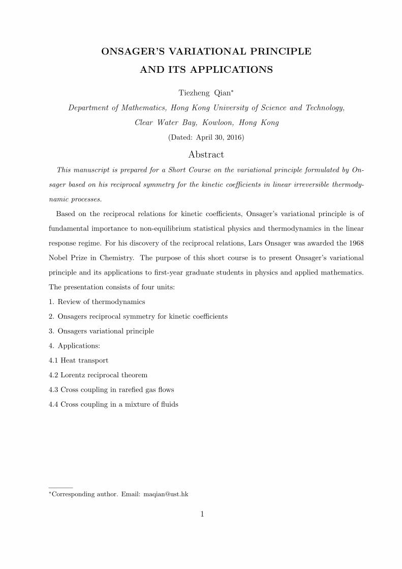
We consider the condition for equilibrium in a system made up of two interconnected sub-

systems, as illustrated in figure 1. Initially the subsystems are separated from each other by

a insulating, rigid, and non-permeable barrier.

Weakly interacting quasi-closed subsystems: In the following discussion, we consider two

weakly interacting quasi-closed subsystems 1 and 2. On the one hand, the two subsystems are

quasi-closed, and hence Sj = Sj(Uj , Vj , Nij) for j = 1, 2 and S = S1 + S2 from the statistical

independence. On the other hand, weak coupling is assumed between the two subsystems. This

allows the whole (closed) system to relax towards complete equilibrium (e.g., via energy transfer

between the two subsystems) if the total entropy is not maximized (with respect to U1 or U2).

1. Thermal equilibrium

Imagine that the barrier is allowed to transmit energy (beginning at one instant of time),

with other inhibitions remaining in effect. If the conditions of the two subsystems 1 and

2 do not change, then they are in thermal equilibrium and the entropy of the total system

must be a maximum with respect to small transfer of energy from one subsystem to the

other. Using the additive property of the entropy,

S = S1 + S2,

we have in equilibrium

δS = δS1 + δS2 = 0,

or

δS =

(∂S1

∂U1

)δU1 +

(∂S2

∂U2

)δU2 = 0.

3

Because the total system is thermally closed and the total energy is constant, i.e., δU =

δU1 + δU2 = 0, we have

δS =

[(∂S1

∂U1

)−(∂S2

∂U2

)]δU1 = 0.

As δU1 is an arbitrary variation, we obtain in thermal equilibrium

∂S1

∂U1

=∂S2

∂U2

.

Defining the temperature T by1

T=

(∂S

∂U

)xν ,Ni

,

we obtain T1 = T2 as the condition for thermal equilibrium.

Suppose that the two subsystems were not originally in thermal equilibrium, but that

T2 > T1. When thermal contact is established to allow energy transmission, the total entropy

S will increase. (The removal of any constraint can only increase the volume of phase space

accessible to the system.) Thus, after thermal contact is established, δS > 0, or[(∂S1

∂U1

)−(∂S2

∂U2

)]δU1 > 0,

and [1

T1

− 1

T2

]δU1 > 0.

Assuming T2 > T1, we have δU1 > 0. This means that energy passes from the system of

high T to the system of low T . So T is indeed a quantity that behaves qualitatively like a

temperature.

2. Mechanical equilibrium

Now imagine that the wall is allowed to move and also transmit energy, but does not pass

particles. The volumes V1 and V2 of the two subsystems can readjust to (further) maximize

the entropy. In mechanical equilibrium

δS =

(∂S1

∂V1

)δV1 +

(∂S2

∂V2

)δV2 +

(∂S1

∂U1

)δU1 +

(∂S2

∂U2

)δU2 = 0.

After thermal equilibrium has been established, we have(∂S1

∂U1

)δU1 +

(∂S2

∂U2

)δU2 = 0.

4

As the total volume V = V1 + V2 is constant, we have δV = δV1 + δV2 = 0, and

δS =

[(∂S1

∂V1

)−(∂S2

∂V2

)]δV1 = 0.

As δV1 is an arbitrary variation, we obtain in mechanical equilibrium

∂S1

∂V1

=∂S2

∂V2

.

Defining the pressure Π byΠ

T=

(∂S

∂V

)U,Ni

,

we see that for a system in thermal equilibrium (with T1 = T2), Π1 = Π2 is the condition for

mechanical equilibrium. In general we define a generalized force Xν related to the coordinate

xν by the equationXν

T=

(∂S

∂xν

)U,Ni

.

It is interesting to note that from the defining equations for T and Π, we obtain

Π =(∂S/∂V )U,Ni

(∂S/∂U)V,Ni

= −(∂U

∂V

)S,Ni

.

This expression for the pressure will be derived again by regarding U as a function of S and

V .

Suppose that the two subsystems in thermal equilibrium were not originally in mechanical

equilibrium, but that Π1 > Π2. When the wall is allowed to move, the total entropy S

will increase. (The removal of any constraint can only increase the volume of phase space

accessible to the system.) From

δS =

[(∂S1

∂V1

)−(∂S2

∂V2

)]δV1 =

1

T[Π1 − Π2] δV1 > 0,

we see that Π1 > Π2 requires δV1 > 0: the subsystem of the higher pressure expands in

volume. So Π is indeed a quantity that behaves qualitatively like a pressure.

3. Particle equilibrium

Now imagine that the wall allows diffusion through it of molecules of the ith chemi-

cal species. Suppose thermal equilibrium and mechanical equilibrium have already been

established. From δNi1 + δNi2 = 0 and

δS =

[(∂S1

∂Ni1

)−(

∂S2

∂Ni2

)]δNi1 = 0,

5

we obtain∂S1

∂Ni1

=∂S2

∂Ni2

,

as the condition for particle equilibrium. Defining the chemical potential µi by

−µi

T=

(∂S

∂Ni

)U,xν

,

we see that for a system in both thermal equilibrium (T1 = T2) and mechanical equilibrium

(Π1 = Π2), µi1 = µi2 is the condition for particle equilibrium. It is easy to show that

particles tend to move from a region of higher chemical potential to that of a lower chemical

potential as the system approaches equilibrium (δS > 0).

C. Connection between statistical and thermodynamical quantities

For a system in equilibrium, S = S(U, xν , Ni), where U is the energy, xν denotes the set

of external parameters describing the system, and Ni is the number of molecules of the i-th

species. If the conditions are changed slightly, but reversibly in such a way that the resulting

system is also in equilibrium, we have

dS =

(∂S

∂U

)dU +

∑ν

(∂S

∂xν

)dxν +

∑i

(∂S

∂Ni

)dNi =

dU

T+

1

T

∑ν

Xνdxν −1

T

∑i

µidNi,

which may be rewritten as

dU = TdS −∑ν

Xνdxν +∑i

µidNi.

Consider that the number of particles is fixed and the volume is the only external parameter:

dNi = 0; xν ≡ V ; Xν ≡ Π. Then,

dU = TdS − ΠdV.

We see that the change of internal energy consists of two parts. The term TdS represents

the change in U when the external parameters are kept constant (dV = 0). This is what we

mean by heat. Thus

DQ = TdS

is the quantity of heat added to the system in a reversible process. The symbol D is used

instead of d because DQ is not an exact differential — that is, Q is not a state function. The

6

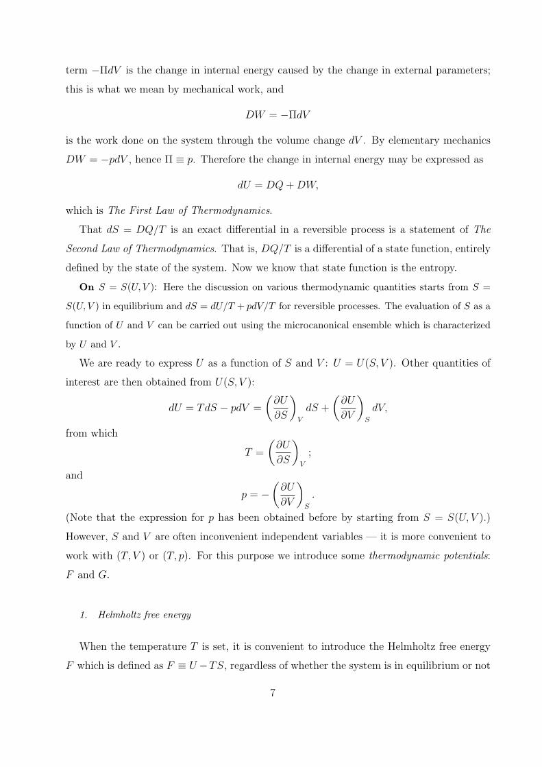
term −ΠdV is the change in internal energy caused by the change in external parameters;

this is what we mean by mechanical work, and

DW = −ΠdV

is the work done on the system through the volume change dV . By elementary mechanics

DW = −pdV , hence Π ≡ p. Therefore the change in internal energy may be expressed as

dU = DQ+DW,

which is The First Law of Thermodynamics.

That dS = DQ/T is an exact differential in a reversible process is a statement of The

Second Law of Thermodynamics. That is, DQ/T is a differential of a state function, entirely

defined by the state of the system. Now we know that state function is the entropy.

On S = S(U, V ): Here the discussion on various thermodynamic quantities starts from S =

S(U, V ) in equilibrium and dS = dU/T + pdV/T for reversible processes. The evaluation of S as a

function of U and V can be carried out using the microcanonical ensemble which is characterized

by U and V .

We are ready to express U as a function of S and V : U = U(S, V ). Other quantities of

interest are then obtained from U(S, V ):

dU = TdS − pdV =

(∂U

∂S

)V

dS +

(∂U

∂V

)S

dV,

from which

T =

(∂U

∂S

)V

;

and

p = −(∂U

∂V

)S

.

(Note that the expression for p has been obtained before by starting from S = S(U, V ).)

However, S and V are often inconvenient independent variables — it is more convenient to

work with (T, V ) or (T, p). For this purpose we introduce some thermodynamic potentials:

F and G.

1. Helmholtz free energy

When the temperature T is set, it is convenient to introduce the Helmholtz free energy

F which is defined as F ≡ U −TS, regardless of whether the system is in equilibrium or not

7

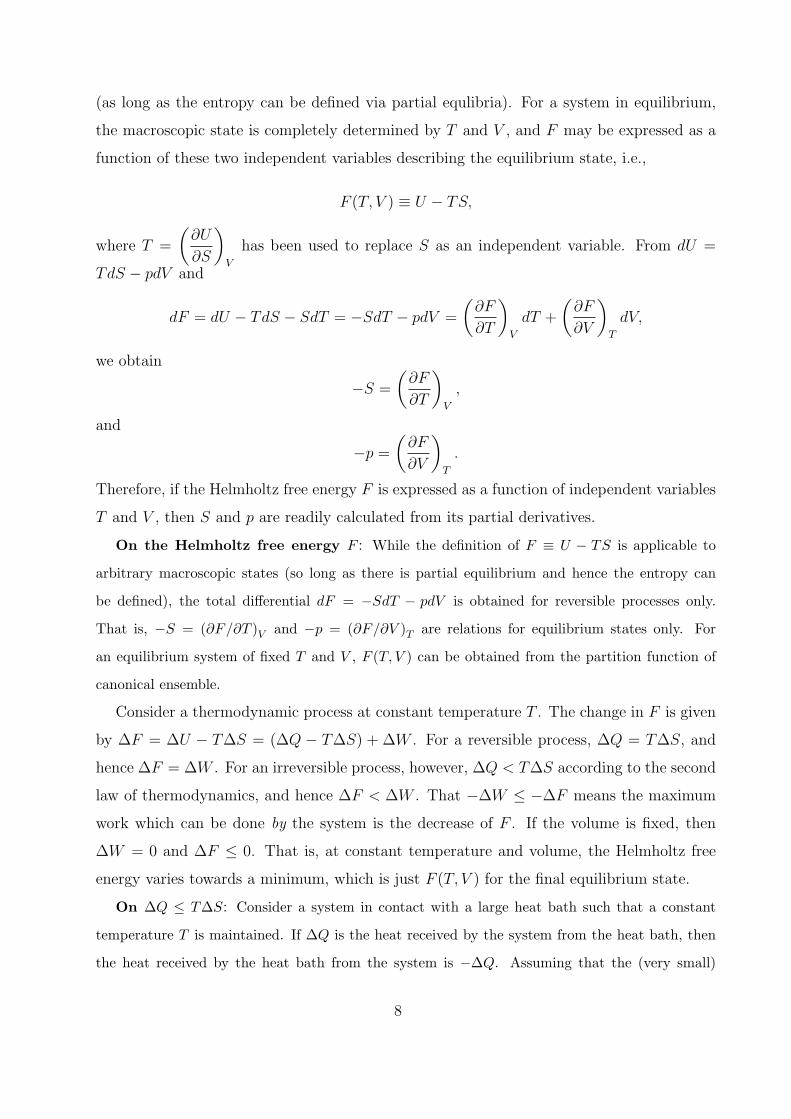
(as long as the entropy can be defined via partial equlibria). For a system in equilibrium,

the macroscopic state is completely determined by T and V , and F may be expressed as a

function of these two independent variables describing the equilibrium state, i.e.,

F (T, V ) ≡ U − TS,

where T =

(∂U

∂S

)V

has been used to replace S as an independent variable. From dU =

TdS − pdV and

dF = dU − TdS − SdT = −SdT − pdV =

(∂F

∂T

)V

dT +

(∂F

∂V

)T

dV,

we obtain

−S =

(∂F

∂T

)V

,

and

−p =

(∂F

∂V

)T

.

Therefore, if the Helmholtz free energy F is expressed as a function of independent variables

T and V , then S and p are readily calculated from its partial derivatives.

On the Helmholtz free energy F : While the definition of F ≡ U − TS is applicable to

arbitrary macroscopic states (so long as there is partial equilibrium and hence the entropy can

be defined), the total differential dF = −SdT − pdV is obtained for reversible processes only.

That is, −S = (∂F/∂T )V and −p = (∂F/∂V )T are relations for equilibrium states only. For

an equilibrium system of fixed T and V , F (T, V ) can be obtained from the partition function of

canonical ensemble.

Consider a thermodynamic process at constant temperature T . The change in F is given

by ∆F = ∆U − T∆S = (∆Q − T∆S) + ∆W . For a reversible process, ∆Q = T∆S, and

hence ∆F = ∆W . For an irreversible process, however, ∆Q < T∆S according to the second

law of thermodynamics, and hence ∆F < ∆W . That −∆W ≤ −∆F means the maximum

work which can be done by the system is the decrease of F . If the volume is fixed, then

∆W = 0 and ∆F ≤ 0. That is, at constant temperature and volume, the Helmholtz free

energy varies towards a minimum, which is just F (T, V ) for the final equilibrium state.

On ∆Q ≤ T∆S: Consider a system in contact with a large heat bath such that a constant

temperature T is maintained. If ∆Q is the heat received by the system from the heat bath, then

the heat received by the heat bath from the system is −∆Q. Assuming that the (very small)

8

change in the (very large) heat bath is reversible, we have −∆Q/T as the change of its entropy.

That the total entropy tends to increase means −∆Q/T +∆S ≥ 0, i.e., ∆Q ≤ T∆S.

2. Gibbs free energy

When the temperature T and the pressure p are both set, it is convenient to introduce

the Gibbs free energy G which is defined as G ≡ F + pV ≡ U − TS + pV , regardless of

whether the system is in equilibrium or not (as long as the entropy can be defined via partial

equlibria). For a system in equilibrium, the macroscopic state is completely determined by

T and p, and G may be expressed as a function of these two independent variables describing

the equilibrium state, i.e.,

G(T, p) ≡ U − TS + pV,

where T =

(∂U

∂S

)V

and p = −(∂U

∂V

)S

has been used to replace S and V as the two

independent variables. From dU = TdS − pdV and

dG = dU − TdS − SdT + pdV + V dp = −SdT + V dp =

(∂G

∂T

)p

dT +

(∂G

∂p

)T

dp,

we obtain

−S =

(∂G

∂T

)p

,

and

V =

(∂G

∂p

)T

.

Therefore, if the Gibbs free energy G is expressed as a function of independent variables T

and p, then S and V are readily calculated from its partial derivatives.

Consider a thermodynamic process at constant temperature T and pressure p. The change

in G is given by ∆G = ∆U − T∆S + p∆V = (∆Q − T∆S) + ∆W + p∆V = ∆Q − T∆S.

For a reversible process, ∆Q = T∆S, and hence ∆G = 0. For an irreversible process,

∆Q < T∆S, and hence ∆G < 0. Therefore, at constant temperature and pressure, the

Gibbs free energy tends to a minimum. This minimum is G(T, p) for the equilibrium state

at the given temperature and pressure.

9

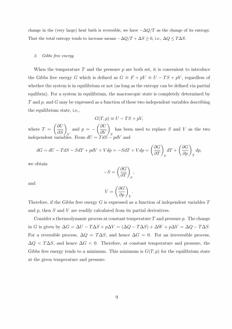
II. ONSAGER’S VARIATIONAL PRINCIPLE

A. Reciprocal relations for linear irreversible thermodynamic processes

The heat flux J induced by temperature gradient ∇T is given by the constitutive equa-

tions

Ji = −3∑

j=1

λij∇jT (i = 1, 2, 3) ,

where λij are coefficients of heat conductivity. The heat conductivity tensor is symmetric

even in crystals of low symmetry (Stokes 1851).

B. Onsager’s reciprocal symmetry derived from microscopic reversibility

For a closed system, consider the fluctuations of a set of (macroscopic) variables

αi (i = 1, ..., n) with respect to their most probable (equilibrium) values. The entropy

of the system S has a maximum Se at equilibrium so that ∆S = S − Se can be written in

the quadratic form,

∆S (α1, ..., αn) = −1

2

n∑i,j=1

βijαiαj,

where β is symmetric and positive definite. The probability density at αi (i = 1, ..., n) is

given by

f (α1, ..., αn) = f (0, ..., 0) e∆S/kB

where kB is the Boltzmann constant. The forces conjugate to αi are defined by

Xi =∂∆S

∂αi

= −n∑

j=1

βijαi

which are linear combinations of αi not far from equilibrium.

Following the above definition of the forces, the equilibrium average (over the distribution

function f (α1, ..., αn) ) of αiXj is given by

⟨αiXj⟩ = −kBδij.

Microscopic reversibility leads to the equality

⟨αi (t)αj (t+ τ)⟩ = ⟨αj (t)αi (t+ τ)⟩

10

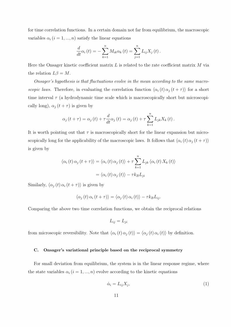
for time correlation functions. In a certain domain not far from equilibrium, the macroscopic

variables αi (i = 1, ..., n) satisfy the linear equations

d

dtαi (t) = −

n∑k=1

Mikαk (t) =n∑

j=1

LijXj (t) .

Here the Onsager kinetic coefficient matrix L is related to the rate coefficient matrix M via

the relation Lβ = M .

Onsager’s hypothesis is that fluctuations evolve in the mean according to the same macro-

scopic laws. Therefore, in evaluating the correlation function ⟨αi (t)αj (t+ τ)⟩ for a short

time interval τ (a hydrodynamic time scale which is macroscopically short but microscopi-

cally long), αj (t+ τ) is given by

αj (t+ τ) = αj (t) + τd

dtαj (t) = αj (t) + τ

n∑k=1

LjkXk (t) .

It is worth pointing out that τ is macroscopically short for the linear expansion but micro-

scopically long for the applicability of the macroscopic laws. It follows that ⟨αi (t)αj (t+ τ)⟩

is given by

⟨αi (t)αj (t+ τ)⟩ = ⟨αi (t)αj (t)⟩+ τ

n∑k=1

Ljk ⟨αi (t)Xk (t)⟩

= ⟨αi (t)αj (t)⟩ − τkBLji

Similarly, ⟨αj (t)αi (t+ τ)⟩ is given by

⟨αj (t)αi (t+ τ)⟩ = ⟨αj (t)αi (t)⟩ − τkBLij.

Comparing the above two time correlation functions, we obtain the reciprocal relations

Lij = Lji

from microscopic reversibility. Note that ⟨αi (t)αj (t)⟩ = ⟨αj (t)αi (t)⟩ by definition.

C. Onsager’s variational principle based on the reciprocal symmetry

For small deviation from equilibrium, the system is in the linear response regime, where

the state variables αi (i = 1, ..., n) evolve according to the kinetic equations

αi = LijXj, (1)

11

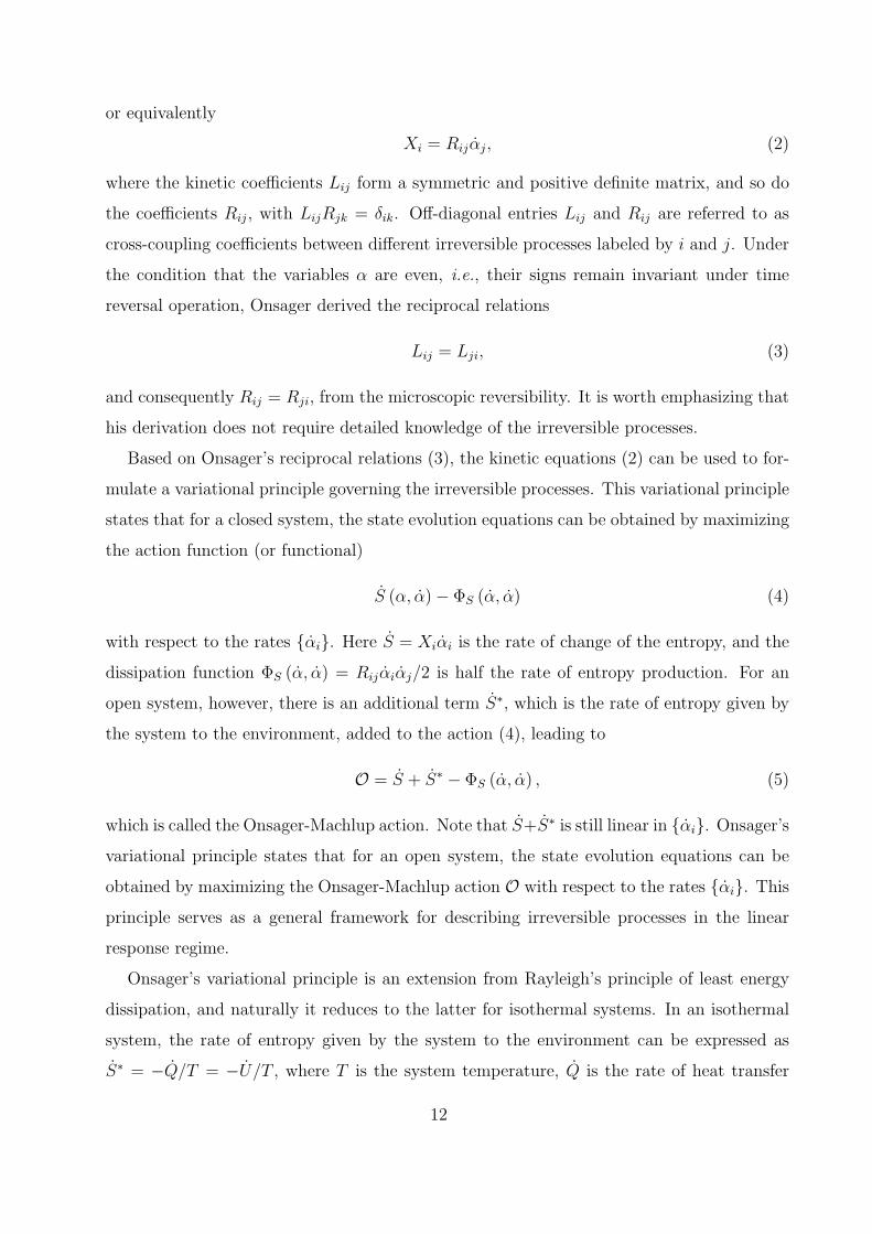
or equivalently

Xi = Rijαj, (2)

where the kinetic coefficients Lij form a symmetric and positive definite matrix, and so do

the coefficients Rij, with LijRjk = δik. Off-diagonal entries Lij and Rij are referred to as

cross-coupling coefficients between different irreversible processes labeled by i and j. Under

the condition that the variables α are even, i.e., their signs remain invariant under time

reversal operation, Onsager derived the reciprocal relations

Lij = Lji, (3)

and consequently Rij = Rji, from the microscopic reversibility. It is worth emphasizing that

his derivation does not require detailed knowledge of the irreversible processes.

Based on Onsager’s reciprocal relations (3), the kinetic equations (2) can be used to for-

mulate a variational principle governing the irreversible processes. This variational principle

states that for a closed system, the state evolution equations can be obtained by maximizing

the action function (or functional)

S (α, α)− ΦS (α, α) (4)

with respect to the rates αi. Here S = Xiαi is the rate of change of the entropy, and the

dissipation function ΦS (α, α) = Rijαiαj/2 is half the rate of entropy production. For an

open system, however, there is an additional term S∗, which is the rate of entropy given by

the system to the environment, added to the action (4), leading to

O = S + S∗ − ΦS (α, α) , (5)

which is called the Onsager-Machlup action. Note that S+S∗ is still linear in αi. Onsager’s

variational principle states that for an open system, the state evolution equations can be

obtained by maximizing the Onsager-Machlup action O with respect to the rates αi. This

principle serves as a general framework for describing irreversible processes in the linear

response regime.

Onsager’s variational principle is an extension from Rayleigh’s principle of least energy

dissipation, and naturally it reduces to the latter for isothermal systems. In an isothermal

system, the rate of entropy given by the system to the environment can be expressed as

S∗ = −Q/T = −U/T , where T is the system temperature, Q is the rate of heat transfer

12

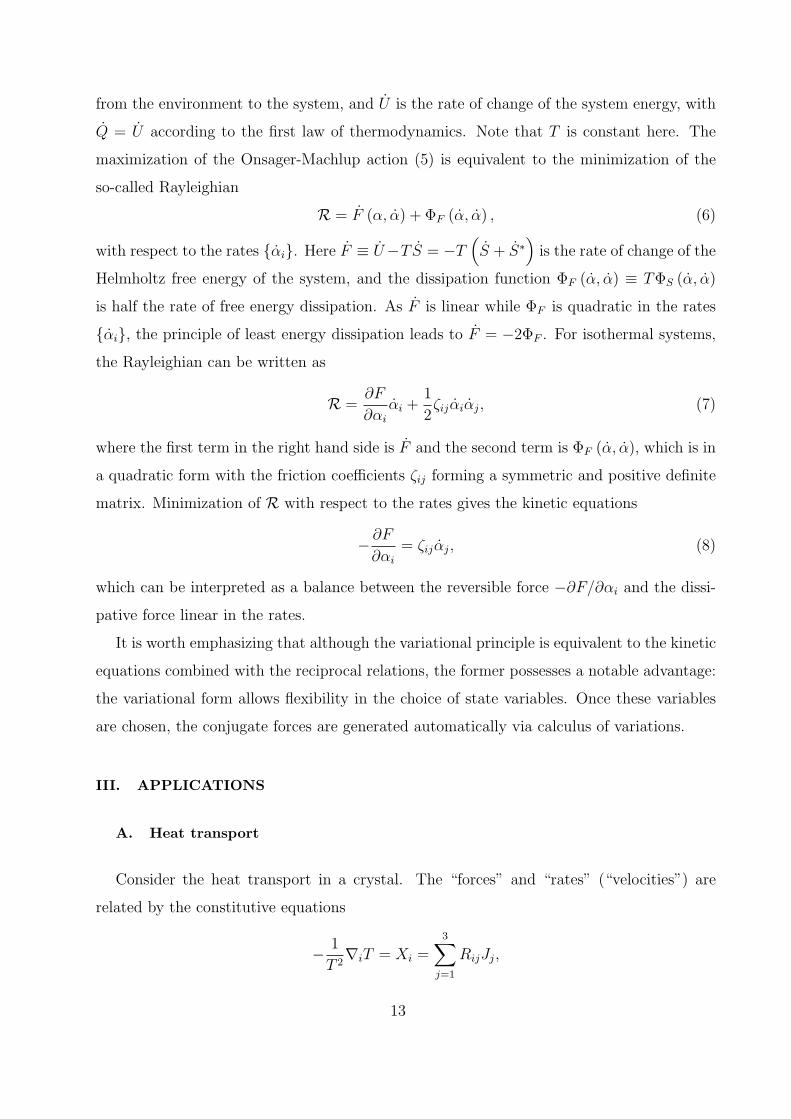
from the environment to the system, and U is the rate of change of the system energy, with

Q = U according to the first law of thermodynamics. Note that T is constant here. The

maximization of the Onsager-Machlup action (5) is equivalent to the minimization of the

so-called Rayleighian

R = F (α, α) + ΦF (α, α) , (6)

with respect to the rates αi. Here F ≡ U−T S = −T(S + S∗

)is the rate of change of the

Helmholtz free energy of the system, and the dissipation function ΦF (α, α) ≡ TΦS (α, α)

is half the rate of free energy dissipation. As F is linear while ΦF is quadratic in the rates

αi, the principle of least energy dissipation leads to F = −2ΦF . For isothermal systems,

the Rayleighian can be written as

R =∂F

∂αi

αi +1

2ζijαiαj, (7)

where the first term in the right hand side is F and the second term is ΦF (α, α), which is in

a quadratic form with the friction coefficients ζij forming a symmetric and positive definite

matrix. Minimization of R with respect to the rates gives the kinetic equations

− ∂F

∂αi

= ζijαj, (8)

which can be interpreted as a balance between the reversible force −∂F/∂αi and the dissi-

pative force linear in the rates.

It is worth emphasizing that although the variational principle is equivalent to the kinetic

equations combined with the reciprocal relations, the former possesses a notable advantage:

the variational form allows flexibility in the choice of state variables. Once these variables

are chosen, the conjugate forces are generated automatically via calculus of variations.

III. APPLICATIONS

A. Heat transport

Consider the heat transport in a crystal. The “forces” and “rates” (“velocities”) are

related by the constitutive equations

− 1

T 2∇iT = Xi =

3∑j=1

RijJj,

13

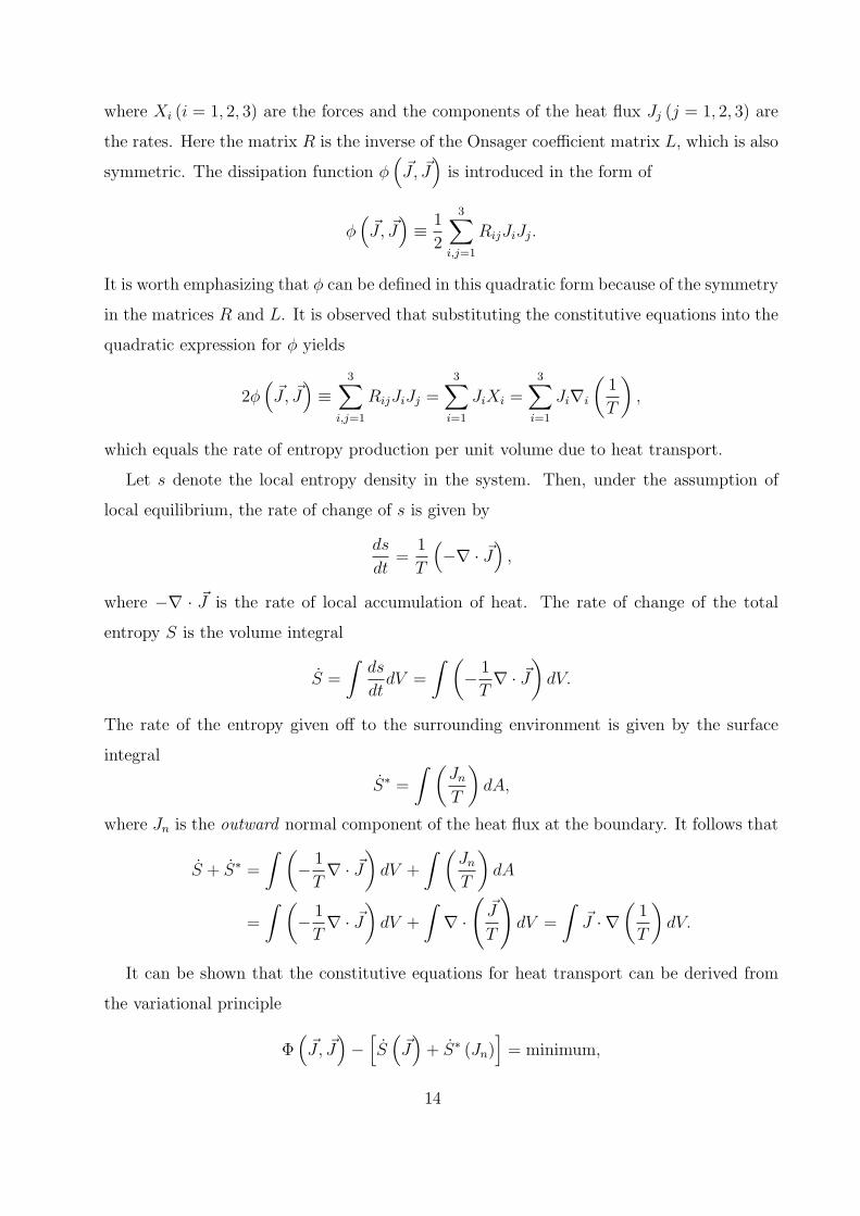
where Xi (i = 1, 2, 3) are the forces and the components of the heat flux Jj (j = 1, 2, 3) are

the rates. Here the matrix R is the inverse of the Onsager coefficient matrix L, which is also

symmetric. The dissipation function ϕ(J , J

)is introduced in the form of

ϕ(J , J

)≡ 1

2

3∑i,j=1

RijJiJj.

It is worth emphasizing that ϕ can be defined in this quadratic form because of the symmetry

in the matrices R and L. It is observed that substituting the constitutive equations into the

quadratic expression for ϕ yields

2ϕ(J , J

)≡

3∑i,j=1

RijJiJj =3∑

i=1

JiXi =3∑

i=1

Ji∇i

(1

T

),

which equals the rate of entropy production per unit volume due to heat transport.

Let s denote the local entropy density in the system. Then, under the assumption of

local equilibrium, the rate of change of s is given by

ds

dt=

1

T

(−∇ · J

),

where −∇ · J is the rate of local accumulation of heat. The rate of change of the total

entropy S is the volume integral

S =

∫ds

dtdV =

∫ (− 1

T∇ · J

)dV.

The rate of the entropy given off to the surrounding environment is given by the surface

integral

S∗ =

∫ (JnT

)dA,

where Jn is the outward normal component of the heat flux at the boundary. It follows that

S + S∗ =

∫ (− 1

T∇ · J

)dV +

∫ (JnT

)dA

=

∫ (− 1

T∇ · J

)dV +

∫∇ ·

(J

T

)dV =

∫J · ∇

(1

T

)dV.

It can be shown that the constitutive equations for heat transport can be derived from

the variational principle

Φ(J , J

)−[S(J)+ S∗ (Jn)

]= minimum,

14

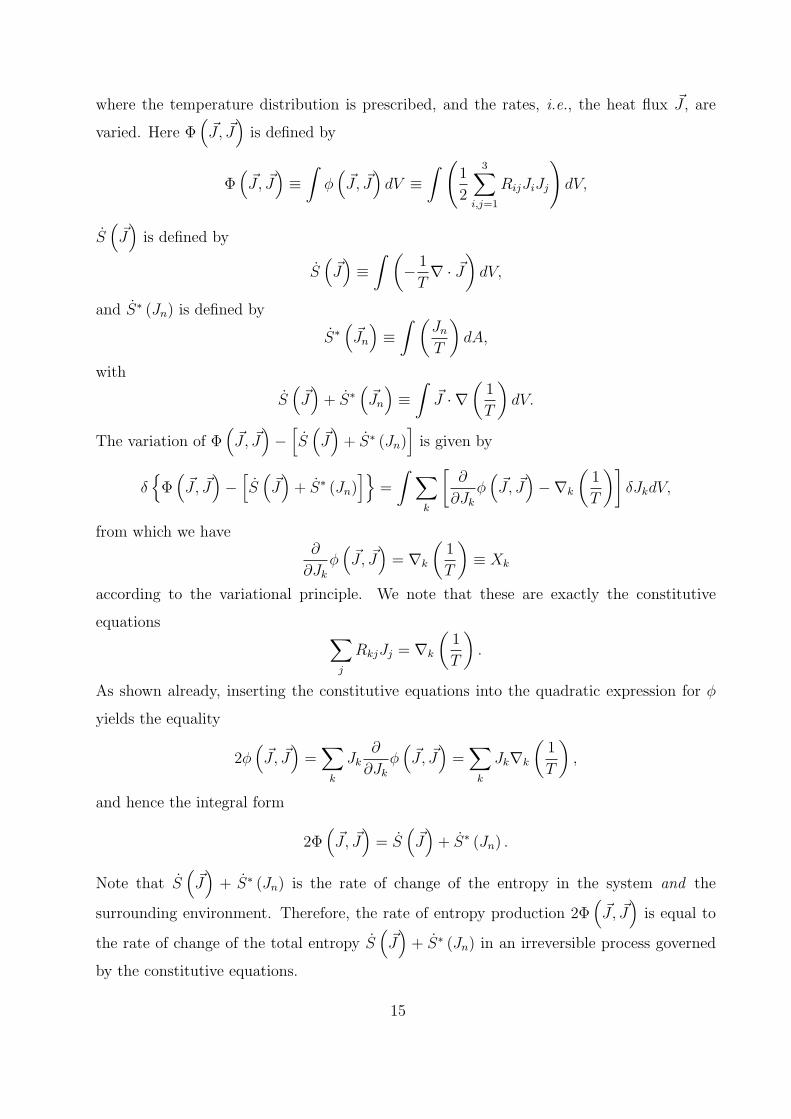
where the temperature distribution is prescribed, and the rates, i.e., the heat flux J , are

varied. Here Φ(J , J

)is defined by

Φ(J , J

)≡∫

ϕ(J , J

)dV ≡

∫ (1

2

3∑i,j=1

RijJiJj

)dV,

S(J)is defined by

S(J)≡∫ (

− 1

T∇ · J

)dV,

and S∗ (Jn) is defined by

S∗(Jn

)≡∫ (

JnT

)dA,

with

S(J)+ S∗

(Jn

)≡∫

J · ∇(1

T

)dV.

The variation of Φ(J , J

)−[S(J)+ S∗ (Jn)

]is given by

δΦ(J , J

)−[S(J)+ S∗ (Jn)

]=

∫ ∑k

[∂

∂Jkϕ(J , J

)−∇k

(1

T

)]δJkdV,

from which we have∂

∂Jkϕ(J , J

)= ∇k

(1

T

)≡ Xk

according to the variational principle. We note that these are exactly the constitutive

equations ∑j

RkjJj = ∇k

(1

T

).

As shown already, inserting the constitutive equations into the quadratic expression for ϕ

yields the equality

2ϕ(J , J

)=∑k

Jk∂

∂Jkϕ(J , J

)=∑k

Jk∇k

(1

T

),

and hence the integral form

2Φ(J , J

)= S

(J)+ S∗ (Jn) .

Note that S(J)+ S∗ (Jn) is the rate of change of the entropy in the system and the

surrounding environment. Therefore, the rate of entropy production 2Φ(J , J

)is equal to

the rate of change of the total entropy S(J)+ S∗ (Jn) in an irreversible process governed

by the constitutive equations.

15

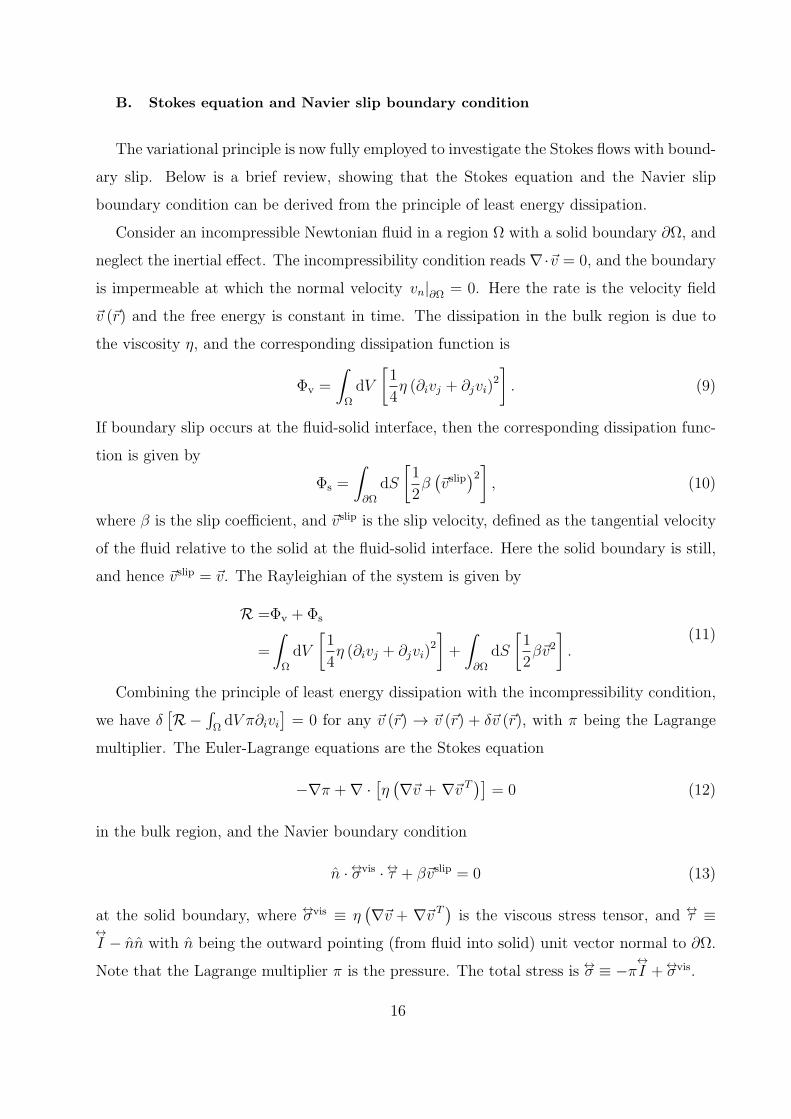
B. Stokes equation and Navier slip boundary condition

The variational principle is now fully employed to investigate the Stokes flows with bound-

ary slip. Below is a brief review, showing that the Stokes equation and the Navier slip

boundary condition can be derived from the principle of least energy dissipation.

Consider an incompressible Newtonian fluid in a region Ω with a solid boundary ∂Ω, and

neglect the inertial effect. The incompressibility condition reads ∇· v = 0, and the boundary

is impermeable at which the normal velocity vn|∂Ω = 0. Here the rate is the velocity field

v (r) and the free energy is constant in time. The dissipation in the bulk region is due to

the viscosity η, and the corresponding dissipation function is

Φv =

∫Ω

dV

[1

4η (∂ivj + ∂jvi)

2

]. (9)

If boundary slip occurs at the fluid-solid interface, then the corresponding dissipation func-

tion is given by

Φs =

∫∂Ω

dS

[1

2β(vslip

)2], (10)

where β is the slip coefficient, and vslip is the slip velocity, defined as the tangential velocity

of the fluid relative to the solid at the fluid-solid interface. Here the solid boundary is still,

and hence vslip = v. The Rayleighian of the system is given by

R =Φv + Φs

=

∫Ω

dV

[1

4η (∂ivj + ∂jvi)

2

]+

∫∂Ω

dS

[1

2βv2].

(11)

Combining the principle of least energy dissipation with the incompressibility condition,

we have δ[R−

∫ΩdV π∂ivi

]= 0 for any v (r) → v (r) + δv (r), with π being the Lagrange

multiplier. The Euler-Lagrange equations are the Stokes equation

−∇π +∇ ·[η(∇v + ∇v T

)]= 0 (12)

in the bulk region, and the Navier boundary condition

n · σ↔vis · τ↔+ βvslip = 0 (13)

at the solid boundary, where σ↔vis ≡ η(∇v + ∇v T

)is the viscous stress tensor, and τ↔ ≡

I↔− nn with n being the outward pointing (from fluid into solid) unit vector normal to ∂Ω.

Note that the Lagrange multiplier π is the pressure. The total stress is σ↔ ≡ −πI↔+ σ↔vis.

16

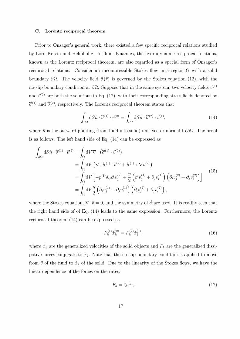
C. Lorentz reciprocal theorem

Prior to Onsager’s general work, there existed a few specific reciprocal relations studied

by Lord Kelvin and Helmholtz. In fluid dynamics, the hydrodynamic reciprocal relations,

known as the Lorentz reciprocal theorem, are also regarded as a special form of Onsager’s

reciprocal relations. Consider an incompressible Stokes flow in a region Ω with a solid

boundary ∂Ω. The velocity field v (r) is governed by the Stokes equation (12), with the

no-slip boundary condition at ∂Ω. Suppose that in the same system, two velocity fields v(1)

and v(2) are both the solutions to Eq. (12), with their corresponding stress fields denoted by

σ↔(1) and σ↔(2), respectively. The Lorentz reciprocal theorem states that∫∂Ω

dSn · σ↔(1) · v(2) =∫∂Ω

dSn · σ↔(2) · v(1), (14)

where n is the outward pointing (from fluid into solid) unit vector normal to ∂Ω. The proof

is as follows. The left hand side of Eq. (14) can be expressed as∫∂Ω

dSn · σ↔(1) · v(2) =∫Ω

dV∇ ·(σ↔(1) · v(2)

)=

∫Ω

dV(∇ · σ↔(1) · v(2) + σ↔(1) : ∇v(2)

)=

∫Ω

dV[−p(1)δij∂iv

(2)j +

η

2

(∂iv

(1)j + ∂jv

(1)i

)(∂iv

(2)j + ∂jv

(2)i

)]=

∫Ω

dVη

2

(∂iv

(1)j + ∂jv

(1)i

)(∂iv

(2)j + ∂jv

(2)i

),

(15)

where the Stokes equation, ∇· v = 0, and the symmetry of σ↔ are used. It is readily seen that

the right hand side of of Eq. (14) leads to the same expression. Furthermore, the Lorentz

reciprocal theorem (14) can be expressed as

F(1)k x

(2)k = F

(2)k x

(1)k , (16)

where xk are the generalized velocities of the solid objects and Fk are the generalized dissi-

pative forces conjugate to xk. Note that the no-slip boundary condition is applied to move

from v of the fluid to xk of the solid. Due to the linearity of the Stokes flows, we have the

linear dependence of the forces on the rates:

Fk = ζklxl, (17)

17

where the friction coefficients ζkl form a positive definite matrix. It follows from Eq. (16)

that the Lorentz reciprocal theorem can be expressed as

ζkl = ζlk, (18)

meaning that the matrix formed by the friction coefficients ζkl is symmetric.

In the above discussion, the Lorentz reciprocal theorem expressed in Eqs. (16) and (18)

is derived from the Stokes equation and the no-slip boundary condition. We have already

shown that the Stokes equation (12) and the Navier boundary condition (13) can be simul-

taneously obtained from the principle of least energy dissipation. It is therefore expected

that the hydrodynamic reciprocal relations can be generalized to describe the Stokes flows

with the Navier boundary condition.

Consider the same system with the Navier boundary condition. The velocity of the solid

boundary ∂Ω is denoted by W . From the Navier boundary condition (13), we readily obtain∫∂Ω

dSn · σ↔(1) · vslip(2) =∫∂Ω

dSn · σ↔(2) · vslip(1). (19)

Meanwhile, Eq. (14) still holds. Note that W = v − vslip on ∂Ω. By combining Eqs. (14)

and (19), we obtain the generalized form of the hydrodynamic reciprocal relations∫∂Ω

dSn · σ↔(1) · W (2) =

∫∂Ω

dSn · σ↔(2) · W (1). (20)

Note that the no-slip limit is obtained as β → ∞ with W = v on ∂Ω. With the Lorentz

reciprocal theorem generalized from Eq. (14) to (20), it can be further expressed as Eq. (16),

which results in the symmetry in Eq. (18). We emphasize that in the presence of boundary

slip, we need Eq. (20) in order to arrive at Eqs. (16) and (18). It is remarkable that the

reciprocal symmetry is preserved in the Stokes flows with the Navier slip condition.

To use Eq. (18) for the present study, we consider the solid boundary ∂Ω consisting of the

surfaces of N rigid bodies ∂Ωi (i = 1, ..., N), each in a motion described by the translational

velocity V i and the angular velocity ωi. The solid velocity at r on ∂Ωi can be expressed as

W (r) = V i + ωi × δri (21)

where δri is measured relative to the center of mass of the i-th rigid body. Then we have∫∂Ω

dSn · σ↔(1) · W (2)

=N∑i=1

(∫∂Ωi

dSn · σ↔(1)

)· V i(2) +

N∑i=1

[∫∂Ωi

dSδri ×(n · σ↔(1)

)]· ωi(2),

18

where∫∂Ωi dSn·σ↔ is the total force by the i-th rigid body on the fluid, and

∫∂Ωi dSδr

i×(n · σ↔)

is the total torque by the i-th rigid body on the fluid. This leads to a specific form of Eq. (16),

in which V i and ωi (i = 1, ..., N) are the generalized velocities of the rigid bodies xk, and∫∂Ωi dSn · σ↔ and

∫∂Ωi dSδr

i × (n · σ↔) are their conjugate generalized forces Fk.

Finally we emphasize that the Lorentz reciprocal theorem is valid only when the slip

length ls = η/β is a material constant, which makes the Navier boundary condition linear.

D. Nematic liquid crystals

The Leslie-Ericksen hydrodynamic theory for nematic liquid crystals gives the dissipative

stress tensor σ↔ and the torque density by the director on the fluid Γ as

σ↔ =α1

(nn :

↔A)nn+ α2nN + α3N n+ α4

↔A+ α5n

(n ·

↔A)+ α6

(n ·

↔A)n, (22)

Γ = n×(γ1N + γ2

↔A · n

), (23)

where αi (i = 1, ..., 6) are phenomenological parameters, n is the director,↔A ≡ 1

2

(∇v + ∇v T

)is the rate-of-strain tensor of flow, and N ≡ ˙n− ν × n = (ω − ν)× n is the velocity of the

director relative to the fluid, with ω being the angular velocity of the director and ν ≡ 12∇×v

being the angular velocity of the fluid. In addition, γ1 and γ2 are given by γ1 = α3−α2 and

γ2 = α6 − α5. Only five of the six αi (i = 1, ..., 6) parameters are independent because of

the Parodi relation

α2 + α3 = α6 − α5, (24)

which results from the Onsager reciprocal relations.

E. Cross coupling in gas flows in micro-channels

In rarefied gases, mass and heat transport processes interfere with each other, leading to

the mechano-caloric effect and thermo-osmotic effect, which are of interest to both theoretical

study and practical applications. We employ the unified gas-kinetic scheme to investigate

these cross coupling effects in gas flows in micro-channels. Our numerical simulations cover

channels of planar surfaces and also channels of ratchet surfaces, with Onsager’s reciprocal

relation verified for both cases. For channels of planar surfaces, simulations are performed

in a wide range of Knudsen number and our numerical results show good agreement with

19

the literature results. For channels of ratchet surfaces, simulations are performed for both

the slip and transition regimes and our numerical results not only confirm the theoretical

prediction [Phys. Rev. Lett. 107, 164502 (2011)] for Knudsen number in the slip regime but

also show that the off-diagonal kinetic coefficients for cross coupling effects are maximized

at a Knudsen number in the transition regime. Finally, a preliminary optimization study is

carried out for the geometry of Knudsen pump based on channels of ratchet surfaces.

In a closed system out of equilibrium, the rate of entropy production can be expressed as

dS

dt=

N∑i=1

JiXi, (25)

where S is the entropy, Ji are the thermodynamic fluxes, and Xi are the conjugate ther-

modynamic forces. For small deviation away from equilibrium, we have the linear relations

between Ji and Xi:

Ji =N∑j=1

LijXj, (26)

where Lij are the kinetic coefficients. Onsager’s reciprocal relations state that Lij and Lji

are equal as a result of microscopic reversibility. Starting from the Gibbs equation, the

thermodynamic fluxes and forces can be identified for gas flows, and the corresponding

constitutive equations can be derived.

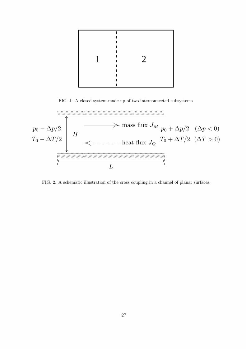
A schematic illustration of the cross coupling in a channel of planar surfaces can be

found in figure 2, where a long channel is confined by two parallel solid plates separated by

a distance H and connected with two reservoirs. The left reservoir is maintained at pressure

p0 −∆p/2 and temperature T0 −∆T/2 while the right reservoir is maintained at p0 +∆p/2

and T0 + ∆T/2. We use ∆p < 0 and ∆T > 0 in our simulations, with |∆p/p0| ≪ 1 and

|∆T/T0| ≪ 1 to ensure the linear response. Usually, a mass flux to the right is generated

by the pressure gradient due to ∆p < 0 and a heat flux to the left is generated by the

temperature gradient due to ∆T > 0. For rarefied gas, however, ∆p also contributes to the

heat flux and ∆T also contributes to the mass flux. These cross coupling effects are called

the mechano-caloric effect and thermo-osmotic effect respectively.

For a single-component gas, the rate of entropy production can be expressed as

dS

dt= JM∆

(− ν

T

)+ JE∆

(1

T

), (27)

where ν is the chemical potential per unit mass, JE and JM are the energy flux and mass

flux from the left reservoir to the right reservoir, and ∆ means the quantity on the right

20

minus the quantity on the left. Here ν and JE can be written as

ν = h− Ts, (28)

JE = JQ + hJM , (29)

where s and h are the entropy and enthalpy per unit mass, and JQ is the heat flux. Together

with the Gibbs-Duhem equation

dν = −sdT + dp/ρ, (30)

where ρ is the mass density. Equation (27) becomes

dS

dt= − 1

ρTJM∆p− 1

T 2JQ∆T. (31)

According to equation (31), the thermodynamic forces and fluxes are connected in the

form of JMJQ

=

LMM LMQ

LQM LQQ

−ρ−10 T−1

0 ∆p

−T−20 ∆T

, (32)

with

LMQ = LQM , (33)

due to Onsager’s reciprocal relations. The detailed mechanism may vary with geometric

configuration and rarefaction. Here and throughout the paper, the subscript ‘0’ denotes the

reference state from which various deviations (in pressure, temperature, etc) are measured.

In the free molecular regime and with specular reflection on plates, the gas molecules

travel ballistically from on side to the other and the distribution function at any point can

be treated as a combination of two half-space Maxwellians from the two reservoirs. The

kinetic coefficients in equation (32) can be analytically derived in this case, given byLMM LMQ

LQM LQQ

=

Hρ0T0

4

√8kBT0

πm

ρ0/p0 −1/2

−1/2 9p0/4ρ0

.

(34)

where kB is the Boltzmann constant and m is the molecular mass.

If the temperature gradient is imposed on the plates and the gas molecules are diffusely

reflected, then the mass flux due to the temperature gradient is generated by thermal creep

21

on the plates. The kinetic coefficients in this case have been calculated by several authors

using different methods. Assuming the length to height ratio of the channel is fixed and

noting ρλ = constant and µ ∝ ρ0T 1/2 for hard-sphere molecules, the average velocity U

induced by thermal creep can be estimated from the Maxwell slip boundary condition,

U ∼ µ0

ρ0T0

∇T ∝ Kn∆T√T0

, (35)

where λ is the mean free path, µ is the dynamic viscosity independent of the density, and

Kn = λ0/H is the Knudsen number. In later sections, we will show that LMQ and LQM are

equal and increase with the increasing Kn.

F. Cross coupling in a mixture of fluids

1. Ideal fluids

The continuity equation is given by

∂

∂tρ+∇ · (ρv) = 0

where ρ is the mass density. The momentum equation is given by

∂

∂t(ρv) +∇ · (ρvv) = ρ

d

dtv = −∇p

where ddtv ≡ ∂

∂tv + v · ∇v is the rate of change of the velocity of a given fluid particle, and

p is the pressure. This is Euler’s equation and is one of the fundamental equations of fluid

dynamics. The motion of an ideal fluid is adiabatic and in adiabatic motion the entropy

of any fluid particle remains constant as the particle moves about in space. Therefore, the

entropy equation is given by∂

∂t(ρs) +∇ · (ρsv) = 0

where s is the entropy per unit mass.

Now we are ready to derive the energy equation. The kinetic energy density is 12ρv2 and

the internal energy density is ρε where ε is the internal energy per unit mass. Using the

continuity equation and the momentum equation, we have

∂

∂t

(1

2ρv2)

= −v · ∇p−∇ ·[(

1

2ρv2)v

]22

for the kinetic energy. As to the internal energy, we have d (ρε) = ρTds + hdρ where

h = ε+ p/ρ is the enthalpy per unit mass. It follows that for an ideal fluid we have

∂

∂t(ρε) = ρT

∂

∂ts+ h

∂

∂tρ = −ρT v · ∇s− h∇ · (ρv)

by use of the entropy equation and the continuity equation. Putting the two energies to-

gether, we have

∂

∂t

(1

2ρv2 + ρε

)= −v · ∇p−∇ ·

[(1

2ρv2)v

]− ρT v · ∇s− h∇ · (ρv) .

To proceed, we note that from thermodynamics we have dh = Tds+(1/ρ)dp, ρdh = ρTds+

dp, and hence ρ∇h = ρT∇s+∇p. It follows that ∂∂t

(12ρv2 + ρε

)can be expressed as

∂

∂t

(1

2ρv2 + ρε

)= −∇ ·

[(1

2ρv2 + ρh

)v

],

which shows that the energy flux is given by(12ρv2 + ρh

)v. Note that we have ρhv rather

than ρεv in the energy flux because the work done by pressure forces is to be included.

2. Viscous fluids

Now we turn to viscous fluids. The continuity equation remains unchanged and the

momentum equation is given by

∂

∂t(ρv) +∇ · (ρvv) = ρ

d

dtv = −∇p+∇ · ↔σ

′

where↔σ′is the viscous stress tensor. The energy equation is given by

∂

∂t

(1

2ρv2 + ρε

)= −∇ ·

[(1

2ρv2 + ρh

)v

]+∇ ·

(↔σ′· v)−∇ · q

where q is the heat flux. Note that the energy equation for viscous fluids takes into account

the work done by viscous forces and the thermal conduction, which are absent in ideal fluids.

The entropy equation can be derived by use of the above equations and thermodynamic

relations. The derivation is straightforward and the procedure can be outlined as follows.

Using the continuity equation and the momentum equation, we can obtain an equation for

∂∂t

(12ρv2). Combining the energy equation and the equation for ∂

∂t

(12ρv2), we can obtain an

equation for ∂∂t(ρε):

∂

∂t(ρε) = −∇ · (ρhv) + ↔

σ′: ∇v −∇ · q + v · ∇p.

23

Combining the above equation with ∂∂t(ρε) = ρT ∂

∂ts+ h ∂

∂tρ, we obtain

ρT∂

∂ts =

↔σ′: ∇v −∇ · q + v · ∇p− ρv · ∇h,

which becomes

ρT

(∂

∂ts+ v · ∇s

)=

↔σ′: ∇v −∇ · q,

with the help of −ρ∇h+∇p = −ρT∇s. Finally we obtain the entropy equation

∂

∂t(ρs) +∇ · (ρsv) = −∇ ·

(q

T

)+

1

T

↔σ′: ∇v + q · ∇ 1

T,

where qT

is the entropy flux, 1T

↔σ′: ∇v is the rate of entropy production due to viscous

dissipation, and q · ∇ 1Tis the rate of entropy production due to thermal conduction.

3. A mixture of fluids

Let us start from the continuity equations of two miscible components, with one labeled

by the subscript “1” and the other labeled by the subscript “2”. They read

∂

∂tρ1 +∇ · (ρ1v1) = 0

and∂

∂tρ2 +∇ · (ρ2v2) = 0,

in which vi (i = 1, 2) is the velocity of a particular species. The mass density ρ and velocity

v of the mixture are defined by ρ = ρ1 + ρ2 and ρv = ρ1v1 + ρ2v2. Physically, v is the mass-

averaged velocity which is a field variable that enters into the hydrodynamic momentum

equation. The local relative concentration c is defined by ρc = ρ1 − ρ2. It follows that ρcv

equals (ρ1 − ρ2)v.

Adding the continuity equations for the two components gives the continuity equation

∂

∂tρ+∇ · (ρv) = 0

for ρ. The diffusive flux j is defined through the equation ρ1v1 − ρ2v2 = ρcv + j. It follows

that j is given by j = ρ1(v1 − v) − ρ2(v2 − v). Note that ρ1(v1 − v) + ρ2(v2 − v) = 0 —

the diffusion discussed here is defined relative to the motion of the center of mass of a fluid

24

element. Rewriting the difference between the continuity equations for the two components

as∂

∂t(ρc) +∇ ·

(ρcv + j

)= 0,

we obtain

ρ

(∂

∂tc+ v · ∇c

)= ρ

d

dtc = −∇ · j.

By introducing µ as an appropriately defined chemical potential of the mixture, we have

thermodynamic equations

d (ρε) = ρTds+ hdρ+ ρµdc

and

ρdh = ρTds+ dp+ ρµdc

for ε and h. They will be used when we derive the entropy equation from the energy equation.

To proceed, we employ the momentum equation

∂

∂t(ρv) +∇ · (ρvv) = ρ

d

dtv = −∇p+∇ · ↔σ

′

and the energy equation

∂

∂t

(1

2ρv2 + ρε

)= −∇ ·

[(1

2ρv2 + ρh

)v

]+∇ ·

(↔σ′· v)−∇ · q,

which look the same as those used for viscous fluids of one component. We would like to

point out that while↔σ′is still the viscous stress tensor, the physical meaning of q is not clear

at the moment — it is expected to represent the total energy flux due to thermal conduction

and diffusion. This is to be clarified by the explicit form of the entropy equation.

In order to derive the entropy equation, we first combine the continuity equation and

the momentum equation to obtain an equation for ∂∂t

(12ρv2). We then combine the energy

equation and the equation for ∂∂t

(12ρv2)to obtain an equation for ∂

∂t(ρε):

∂

∂t(ρε) = −∇ · (ρhv) + ↔

σ′: ∇v −∇ · q + v · ∇p.

Combining the above equation with ∂∂t(ρε) = ρT ∂

∂ts+ h ∂

∂tρ+ ρµ ∂

∂tc from thermodynamics,

we obtain

ρT∂

∂ts =

↔σ′: ∇v −∇ · q + v · ∇p− ρv · ∇h− ρµ

∂

∂tc,

which becomes

ρT

(∂

∂ts+ v · ∇s

)=

↔σ′: ∇v −∇ · q − ρµ

(∂

∂tc+ v · ∇c

),

25

with the help of −ρ∇h+∇p = −ρT∇s− ρµ∇c. Using ρ(

∂∂tc+ v · ∇c

)= −∇ · j, we have

ρT

(∂

∂ts+ v · ∇s

)=

↔σ′: ∇v −∇ · q + µ∇ · j = ↔

σ′: ∇v −∇ ·

(q − µj

)− j · ∇µ,

which gives the entropy equation

∂

∂t(ρs) +∇ · (ρsv) = −∇ ·

(q − µj

T

)+ π,

in which q−µjT

is the entropy flux and π is the rate of entropy production per unit volume,

given by

π =1

T

↔σ′: ∇v +

(q − µj

)· ∇ 1

T− j · ∇µ

T.

Here 1T

↔σ′: ∇v is the rate of entropy production due to viscous dissipation, and

(q − µj

)·

∇ 1T− j · ∇µ

Tis the rate of entropy production due to thermal conduction and diffusion. The

latter can be written as (q − µj

)·(−∇T

T 2

)+ j ·

(−∇µ

T

)in which

(q − µj

)and j are the fluxes associated with thermal conduction and diffusion, and

−∇TT 2 and −∇µ

Tare the conjugate forces. Now we are ready to write down the constitutive

equations

j = −αT

(∇µ

T

)− βT 2

(∇T

T 2

)q − µj = −δT

(∇µ

T

)− γT 2

(∇T

T 2

)with the reciprocal relation βT 2 = δT for the cross coupling between thermal conduction

and diffusion.

FIGURES

26

1 2

FIG. 1. A closed system made up of two interconnected subsystems.

p0 −∆p/2

T0 −∆T/2

p0 +∆p/2

T0 +∆T/2

mass flux JM

heat flux JQ

(∆p < 0)

(∆T > 0)H

L

FIG. 2. A schematic illustration of the cross coupling in a channel of planar surfaces.

27