Embed Size (px)
Citation preview

To link to this article: http://dx.doi.org/10.1080/14685240903273881 URL: http://www.tandfonline.com/doi/abs/10.1080/14685240903273881
This is an author-deposited version published in: http://oatao.univ-toulouse.fr/ Eprints ID: 6326
To cite this version: Cathalifaud, Patricia and Godard, Gilles and Braud, Caroline and Stanislas, Michel The flow structure behind vortex generators embedded in a decelerating turbulent boundary layer. (2009) Journal of Turbulence, vol. 10 (n° 42). pp. 1-37. ISSN 1468-5248
Open Archive Toulouse Archive Ouverte (OATAO) OATAO is an open access repository that collects the work of Toulouse researchers and makes it freely available over the web where possible.
Any correspondence concerning this service should be sent to the repository administrator: [email protected]
The flow structure behind vortex generators embedded in adecelerating turbulent boundary layer
P. Cathalifauda, G. Godardb, C. Braudc and M. Stanislasc∗
aInstitut de Mecanique des Fluides (UMR 5502), UPS, Universite Paul Sabatier, 18, route deNarbonne, 31062 Toulouse Cedex, France; bCORIA (UMR 6614), CNRS, Site Universitaire duMadrillet, 6801 Saint Etienne de Rouvray Cedex, France; cLaboratoire de Mecanique de Lille(UMR 8107), EC Lille, CNRS, Boulevard Paul Langevin, Cite Scientifique, 59655 Villeneuve
d’Ascq Cedex, France
The objective of the present work is to analyse the behaviour of a turbulent deceleratingboundary layer under the effect of both passive and active jets vortex generators (VGs).The stereo PIV database of Godard and Stanislas [1, 2] obtained in an adverse pressuregradient boundary layer is used for this study. After presenting the effect on the meanvelocity field and the turbulent kinetic energy, the line of analysis is extended withtwo points spatial correlations and vortex detection in instantaneous velocity fields.It is shown that the actuators concentrate the boundary layer turbulence in the regionof upward motion of the flow, and segregate the near-wall streamwise vortices of theboundary layer based on their vorticity sign.
Keywords: flow control, vortex generators, turbulent boundary layer, adverse pressuregradient, PIV, coherent structures
1. Introduction
Delaying or preventing turbulent boundary layer (TBL) separation in aeronautic applications(during landing or manoeuvre of an aircraft for example) leads to enhance the lift to dragratio and thus to fuel saving and reduction of the emitted pollution. It allows also to extendthe flight envelop of an aircraft. For that purpose many actuator types were explored in thelast decades over many flow configurations (flat plates, ramps, bumps, ducts, airfoils, windturbines, etc.) [3].
Among the actuators used for that purpose, the vortex generators (VGs) were foundefficient to reduce and sometimes even suppress the separated region [4]. These devicesgenerate a streamwise vortex structure which can entrain high-momentum fluid towardsthe wall, hence energising the TBL, increasing quantities such as wall shear stress, tur-bulence intensities, momentum transfer, etc. and delaying separation. The optimal devicewould produce streamwise vortices just strong enough to overcome the separation withoutpersisting within the boundary layer once the flow control objective is reached. It can beeither passive or active. The resulting streamwise vortices have been subjected to manystudies which helped to characterise the optimal actuator parameters and the resulting meanorganisation. However, too few studies were performed on the flow re-organisation due tothe difficulty to get a sufficient spatial resolution in the TBL.
∗Corresponding author. Email: [email protected]
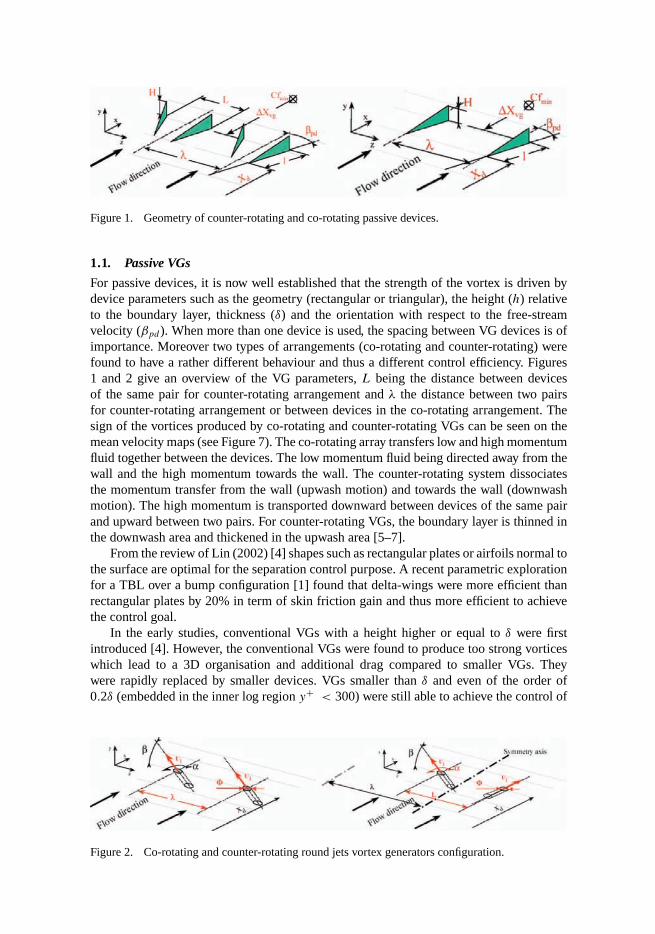
Figure 1. Geometry of counter-rotating and co-rotating passive devices.
1.1. Passive VGs
For passive devices, it is now well established that the strength of the vortex is driven bydevice parameters such as the geometry (rectangular or triangular), the height (h) relativeto the boundary layer, thickness (δ) and the orientation with respect to the free-streamvelocity (βpd ). When more than one device is used, the spacing between VG devices is ofimportance. Moreover two types of arrangements (co-rotating and counter-rotating) werefound to have a rather different behaviour and thus a different control efficiency. Figures1 and 2 give an overview of the VG parameters, L being the distance between devicesof the same pair for counter-rotating arrangement and λ the distance between two pairsfor counter-rotating arrangement or between devices in the co-rotating arrangement. Thesign of the vortices produced by co-rotating and counter-rotating VGs can be seen on themean velocity maps (see Figure 7). The co-rotating array transfers low and high momentumfluid together between the devices. The low momentum fluid being directed away from thewall and the high momentum towards the wall. The counter-rotating system dissociatesthe momentum transfer from the wall (upwash motion) and towards the wall (downwashmotion). The high momentum is transported downward between devices of the same pairand upward between two pairs. For counter-rotating VGs, the boundary layer is thinned inthe downwash area and thickened in the upwash area [5–7].
From the review of Lin (2002) [4] shapes such as rectangular plates or airfoils normal tothe surface are optimal for the separation control purpose. A recent parametric explorationfor a TBL over a bump configuration [1] found that delta-wings were more efficient thanrectangular plates by 20% in term of skin friction gain and thus more efficient to achievethe control goal.
In the early studies, conventional VGs with a height higher or equal to δ were firstintroduced [4]. However, the conventional VGs were found to produce too strong vorticeswhich lead to a 3D organisation and additional drag compared to smaller VGs. Theywere rapidly replaced by smaller devices. VGs smaller than δ and even of the order of0.2δ (embedded in the inner log region y+ < 300) were still able to achieve the control of
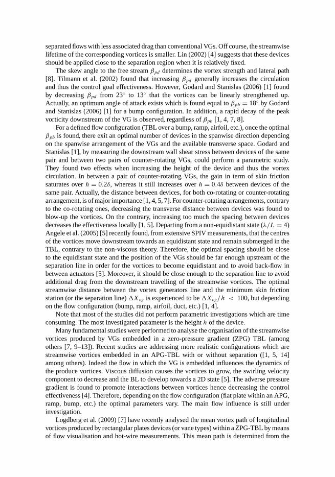
Figure 2. Co-rotating and counter-rotating round jets vortex generators configuration.
separated flows with less associated drag than conventional VGs. Off course, the streamwiselifetime of the corresponding vortices is smaller. Lin (2002) [4] suggests that these devicesshould be applied close to the separation region when it is relatively fixed.
The skew angle to the free stream βpd determines the vortex strength and lateral path[8]. Tilmann et al. (2002) found that increasing βpd generally increases the circulationand thus the control goal effectiveness. However, Godard and Stanislas (2006) [1] foundby decreasing βpd from 23◦ to 13◦ that the vortices can be linearly strengthened up.Actually, an optimum angle of attack exists which is found equal to βpb = 18◦ by Godardand Stanislas (2006) [1] for a bump configuration. In addition, a rapid decay of the peakvorticity downstream of the VG is observed, regardless of βpb [1, 4, 7, 8].
For a defined flow configuration (TBL over a bump, ramp, airfoil, etc.), once the optimalβpb is found, there exit an optimal number of devices in the spanwise direction dependingon the spanwise arrangement of the VGs and the available transverse space. Godard andStanislas [1], by measuring the downstream wall shear stress between devices of the samepair and between two pairs of counter-rotating VGs, could perform a parametric study.They found two effects when increasing the height of the device and thus the vortexcirculation. In between a pair of counter-rotating VGs, the gain in term of skin frictionsaturates over h = 0.2δ, whereas it still increases over h = 0.4δ between devices of thesame pair. Actually, the distance between devices, for both co-rotating or counter-rotatingarrangement, is of major importance [1, 4, 5, 7]. For counter-rotating arrangements, contraryto the co-rotating ones, decreasing the transverse distance between devices was found toblow-up the vortices. On the contrary, increasing too much the spacing between devicesdecreases the effectiveness locally [1, 5]. Departing from a non-equidistant state (λ/L = 4)Angele et al. (2005) [5] recently found, from extensive SPIV measurements, that the centresof the vortices move downstream towards an equidistant state and remain submerged in theTBL, contrary to the non-viscous theory. Therefore, the optimal spacing should be closeto the equidistant state and the position of the VGs should be far enough upstream of theseparation line in order for the vortices to become equidistant and to avoid back-flow inbetween actuators [5]. Moreover, it should be close enough to the separation line to avoidadditional drag from the downstream travelling of the streamwise vortices. The optimalstreamwise distance between the vortex generators line and the minimum skin frictionstation (or the separation line) �Xvg is experienced to be �Xvg/h < 100, but dependingon the flow configuration (bump, ramp, airfoil, duct, etc.) [1, 4].
Note that most of the studies did not perform parametric investigations which are timeconsuming. The most investigated parameter is the height h of the device.
Many fundamental studies were performed to analyse the organisation of the streamwisevortices produced by VGs embedded in a zero-pressure gradient (ZPG) TBL (amongothers [7, 9–13]). Recent studies are addressing more realistic configurations which arestreamwise vortices embedded in an APG-TBL with or without separation ([1, 5, 14]among others). Indeed the flow in which the VG is embedded influences the dynamics ofthe produce vortices. Viscous diffusion causes the vortices to grow, the swirling velocitycomponent to decrease and the BL to develop towards a 2D state [5]. The adverse pressuregradient is found to promote interactions between vortices hence decreasing the controleffectiveness [4]. Therefore, depending on the flow configuration (flat plate within an APG,ramp, bump, etc.) the optimal parameters vary. The main flow influence is still underinvestigation.
Logdberg et al. (2009) [7] have recently analysed the mean vortex path of longitudinalvortices produced by rectangular plates devices (or vane types) within a ZPG-TBL by meansof flow visualisation and hot-wire measurements. This mean path is determined from the

maximum positive value of the mean velocity gradient tensor second invariant at differentstreamwise positions. For a counter-rotating array configuration of VGs, the vortices fromthe same pair first move away from each others. Thus, they move closer to the neighbouringvortex pair and eventually form a new counter-rotating pair with a common flow. Then thevortices move away from the wall. From the authors, this is due to the induced velocity in theupwash motion that tends to lift the vortices. Finally, they move again towards each other,closer to the equidistant-state. The authors attribute this last peculiar hook-like motion tothe vortex growth and the limited space inside the boundary layer due to the neighbouringvortices. The maximum mean vortex radius is estimated to be λ/4 which implies that themean vortex centre path is within a circle defined as followed: y/h = 2.08; z/λ = ±0.25.
Angele et al. [5] and Logdberg [14] also provide a useful rough evaluation of thevortex circulation, γ = 2khUvg/λ, where k is a coefficient that depends on the device used(k = 0.6 for vane-type VG in a ZPG configuration), and Uvg is the streamwise velocity atthe tip of the device. However, this does not include the influence of the skew angle and thecross-flow organisation.
The development of SPIV measurements led to further understanding of the VGs/TBLinteraction. Angele et al. (2005) [5] have recently analysed the VGs/APG-TBL interactionin terms of turbulent properties. In that study the APG induce a small separation area. Theyfound that most of the turbulence production is locally governed by one of the gradientsdU/dy or dU/dz from the S-shape profile of the streamwise velocity in the x-y plane andthe mushroom shape of the streamwise velocity in the y-z plane. In span, between vortices,the spanwise gradient involves significant levels of turbulence production, however the flowis overall more isotropic.
1.2. Active VGs
Passive devices were rapidly replaced by active ones which can be turned off when notnecessary in order to avoid additional drag (i.e. during cruise flight of an aircraft forinstance). Many active device types were then developed for which, depending on thecontrol source used, the control is of different nature (acoustic actuators, plasma actuators,fluidic actuators, etc.). Moreover, within fluidic actuators, one can distinguish syntheticjets devices also called Zero-Net Mass Flux [15–17] and pulsed-jet actuators [18, 19].Indeed, for synthetic jets, contrary to pulsed-jets, there exists a suction phase. Moreover,different jet orifice shapes, orientations and operating parameters (jet oriented normal tothe wall, high or low pulsating frequency, low or high velocity ratios VR between the jetexit velocity and the local free stream velocity, etc.) are used, which lead to different typesof control. For instance, Greenblatt and Wygnansky [20] talk about coherent structuresenhancement also called hydrodynamic control. For this control type, a low VR and apulsating frequency adapted to the natural shedding frequency of the coherent structuresis thought to be efficient. On the other hand, Raman et al. [21] are dealing with the smallturbulent structures; acting one these scales is thought to allow to modify the large scaleorganisation more efficiently than the hydrodynamic control (no development of anotherdominant harmonic).
The present work is focused on control studies using fluidic actuators with addition ofmass to generate streamwise vortices (also called pulsed-jets actuators or pneumatic vortexgenerators).
In continuous mode of the actuator, the streamwise evolution of the produced vorticesby a single active device has been extensively analysed in ZPG configurations ([8, 22, 23]among others). The circulation and the associated strength of the vortex is modified by
parameters such as the ratio between the jet exit velocity and the local free stream velocityVR, the actuator pitch β and skew α angles and the orifice shape (see Figure 2 for notations).Contrary to passive devices, the arrangement may influence significantly the produced jet,leading to additional parameters dependency. Indeed, as highlighted in Peterson et al. [24]and Warsop et al. [25], a separation occurs within the tube (or hole) due to the supplychannel flow shear at the leading or trailing edge of the hole. Warsop et al. [25] foundthis phenomena responsible of pressure losses up to 40% at the exit, whereas Peterson andPlesniak [24] show that for low aspect ratio of the orifice exit (less than unity), the trajectoryand the spanwise spreading of the exit jet can be modified depending on the sign of the‘supply channel-inhole flow”.
Peterson and Plesniak [24] performed an extensive PIV analysis of streamwise vorticesembedded in a TBL (flat plate configuration) for round jet actuators placed perpendicularto the wall. Measurements where taken in the plenum chamber and the exit hole andimmediately downstream the hole. Even if the exit hole was perpendicular to the wall, thisgives insight in the vortex formation mechanism. A single jet perpendicular to a wall givesrise to a pair of counter-rotating streamwise vortices, whereas two inclined jets are neededto get a qualitatively equivalent vortex pair. The origin of the remaining counter-rotatingvortex pair from the jet/free stream interaction is explained by the high shear from the jetedges which induces a roll-up of the boundary layer flow. The shear is more important at thetrailing edge of the hole due to bending of the jet. Behind the jet, a true wake region doesnot develop, but rather the action of the counter-rotating vortex pair draws the fluid awayfrom the wall which creates a recirculation region of low velocity immediately downstreamof the jet along the x-axis. When the blowing ratio increases, the jet lifts from the walland the recirculating region is significantly reduced. Additionally, large separations occurswithin the exit hole of the jet which affects the following development of the two counter-rotating vortices immediately downstream the hole, when the aspect ratio of the exit holeis short (lower than 1). For instance, for a flow in the supply channel pointing in the samedirection as the main flow, the counter-rotating vortices from the jet/free stream interactionare enhanced, up to 35% compared to supply channel pointing in the opposite direction tothe main flow, and thus penetrates further into the TBL. Moreover, the spanwise spreadingslightly decreases, when compared to supply channel pointing in the direction opposite tothe main flow.
When the jet has an angle to the wall (pitch and/or skew angle), two counter-rotatingvortices are initially created just downstream of the device which evolves rapidly into asingle coherent vortex of one sign accompanied by a much smaller and weaker region ofcirculation of the opposite sign near the wall [8]. The performances increase with VR and theeffect is persistent far downstream from the injection (�Xvg/� = 200 or �Xvg/δ = 40).For passive VGs, the primary vortex continues to move laterally in the direction of the vaneskew, while for active VGs the path of the primary vortex is driven by VR. Consequently, toohigh jet exit velocity (VR) can blow the vortices out of the TBL, where it is overwhelmed bythe free-stream momentum and quickly dissipates, hence reducing the control effectiveness[8]. For single VGs embedded in the TBL, the vortices are similar (at least qualitatively) tothe ones from passive VGs [8, 22].
Different VGs arrangements were also investigated [2]. The sign of the produced vor-tices from co-rotating (CO) and counter-rotating (CT) arrangements is found similar to thepassive ones. The CT active VGs are found to produce similar vortices as passive ones inthe same arrangement. On the contrary, CO-active VGs merge more rapidly than passiveones and thus they dissipate more rapidly. The optimal distance between devices was found10-times smaller than for passive devices but with a higher achievable skin friction gain. For
CT actuators, the skin friction gain is proportional to VR with little skin friction gain overVR = 3.1 for a TBL over a bump configuration without separation [2]. Hence, an optimalVR exists over which the vortices may be bleed out of the TBL which wasn’t observed bythe authors. Logdberg [14] found that the necessary VR to achieve the control goal varieslittle with APG. With the assumption that for the same effectiveness criteria, the circulationis identical for both active and passive devices, a rough evaluation of the circulation γ foractive devices was performed. Also, γ = 1.0 to 1.5 was found enough to overcome thesmall separation in all three APG tested. These authors also suggest that an increase of thenumber of jets should be preferred to improve further the control effectiveness rather thanan increase of VR (in the limit of the optimal spacing). For low VR (<4.7) and dependingon the main flow configuration, the optimal skew angle is found between 45◦ and 90◦
[2, 26, 23].The use of active VGs in the pulsed mode enables to decrease further the mass flow
consumption of the actuator. Indeed, in the pulsed mode the pulsating frequency and theDuty Cycle (DC) can be tuned so that successive streamwise vortex segments can mergedownstream, producing quasi-continuous streamwise vortices with less mass flow rate thanthe steady case [8, 19]. Also, depending on the main flow configuration (i.e. attachedor separated TBL over a ramp, bump, etc.) and the actuator-jet strength (VR), the jetpenetration may be modified by the pulsating frequency. Moreover, Tilmann [8] observedthat pulsating the jet always generates a stronger primary vortex independently to thewidth of the DC. More recently, Ortmann and Kaehler, and Kostas et al. [18, 19] founda significant improvement of the control effectiveness during the first millisecond of theactivation/deactivation of the actuator which was related to unsteady oscillations of the jetexit during these phases and subsequent modulation of the primary vortex strength. Theseoscillations were later found to be related to a wave propagation phenomena in the feedingtube of the actuator [27]. The exit jet from the fluid VG was analysed in detailed by [28].However, this is beyond the scope of this paper which treats only the continuous mode ofoperation of active VGs.
These studies allow to conclude on the effectiveness of the actuator and on the meanorganisation of the resulting TBL/VGs interaction. However, too little attention was paid tothe TBL reorganisation behind VGs actuators. This is mainly due to the difficulty to get agood spatial resolution inside the TBL. In the present facility, the TBL is 10-times scaled-up compared to typical experimental facilities which enables to performed a more detailedanalysis of the interaction between the APG-TBL and passive or active VGs. This is doneusing stereo PIV in different planes normal to the flow, downstream of the actuators. Themean flow and turbulent kinetic energy distributions are first characterised. Then a vortexdetection analysis is performed on the instantaneous stereo PIV measurements (see Tables1 and 2). This gives a better insight into the reorganisation of the main flow turbulence inthe presence of streamwise vortices.
Parametric studies of different kinds of vortex generators were performed by Bernardet al. [29], Godard and Stanislas [1] and Godard and Stanislas [2] as part of two Europeanprojects called AEROMEMS and AEROMEMS II. The objectives were to optimise differentactuator systems in order to control separation on an airfoil or a wind flap using MicroElectro-Mechanical Systems (MEMS) technology. Since such systems have very smallscales, an enlargement of the scale of the phenomenon was decided to overcome the problemof spatial resolution. A stereoscopic PIV experiment was also performed by Godard andStanislas [1] and Godard et al [32, 33].
In Section 2, the experiments performed to obtain the present database are described. InSection 3, one point statistical analysis are presented (mean velocity and turbulent kinetic

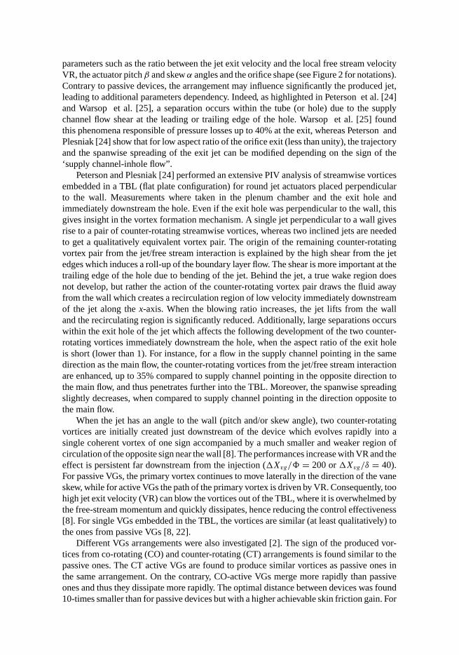
Figure 3. Front view of the TBL wind tunnel.
energy). In Section 4, the spatial correlation is analysed. In Section 5, the vortex detectionmethod and the corresponding results are shown. Finally, a general conclusion is provided.
2. Description of the database
The facility used to acquire the database has the particularity to enable a TBL with δ up to300 mm, fully developed in the test section and characterised in the flat plate configurationby [30]. Some years ago, a bump was added within this TBL. This configuration representsthe non-actuated case. A detailed analysis of this bump flow was performed by Bernardet al. [31]. Later, Godard et al. [1, 2, 32] analysed the effectiveness of different VG devicesfrom an extensive parametric study. Gain in terms of shear stress measurements werecompared and led to optimal configurations. SPIV measurements were then performedon these configurations and briefly described [33]. The same SPIV database is used inthe present analysis with optimal parameters of the devices. To help the reader, someinformation concerning the database is recalled in this section.
2.1. The wind tunnel
Figure 3 is a front view of the boundary layer wind tunnel used. It is 20 m long. The last5 m are transparent on all sides to allow the use of optical methods, and the test section is1 × 2 m2. The free stream velocity for the present database was set at 10 m/s. The windtunnel was used in closed loop to allow the use of smoke. The wind tunnel velocity iscomputer controlled by a PC within ± 0.01%). The boundary layer under study developson the lower wall. It is tripped at the entrance of the tunnel by a grid laid on the floor. Theorigin of the coordinate system is placed in the middle of the lower wall at the entrance ofthe tunnel. The x-axis is parallel to the wall and to the flow, the y-axis is normal to the wall,the reference frame is direct. At the beginning of the bump, x = 15.5 m, the boundary layerthickness is δ = 300 mm.
2.2. The bump
The objective of the AEROMEMS projet was to design a bump with a pressure gradientrepresentative of what happens on the suction side of an airfoil at moderate angle of attackand to approach separation without reaching it in order to prevent the flow to become 3D.The coordinates of the bump can be found in Bernard et al. [31]. The flow in the first halfof the bump strongly accelerates with a rapid variation of the pressure gradient magnitude.At x = 17 m, the sign of the pressure gradient changes and its variation becomes more
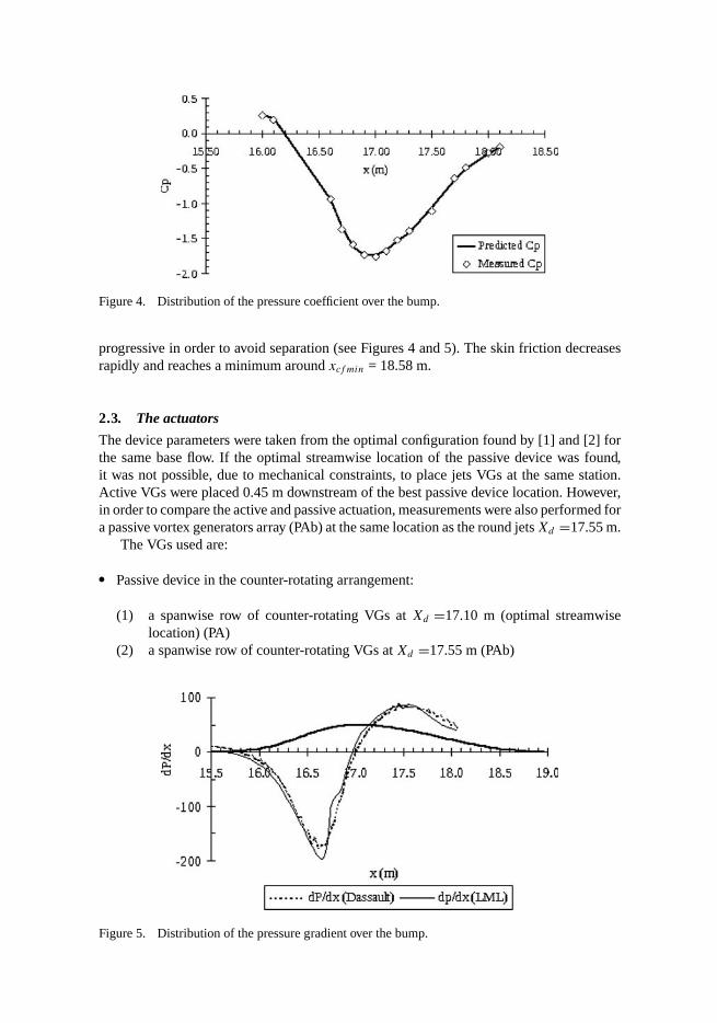
Figure 4. Distribution of the pressure coefficient over the bump.
progressive in order to avoid separation (see Figures 4 and 5). The skin friction decreasesrapidly and reaches a minimum around xcf min = 18.58 m.
2.3. The actuators
The device parameters were taken from the optimal configuration found by [1] and [2] forthe same base flow. If the optimal streamwise location of the passive device was found,it was not possible, due to mechanical constraints, to place jets VGs at the same station.Active VGs were placed 0.45 m downstream of the best passive device location. However,in order to compare the active and passive actuation, measurements were also performed fora passive vortex generators array (PAb) at the same location as the round jets Xd =17.55 m.
The VGs used are:
� Passive device in the counter-rotating arrangement:
(1) a spanwise row of counter-rotating VGs at Xd =17.10 m (optimal streamwiselocation) (PA)
(2) a spanwise row of counter-rotating VGs at Xd =17.55 m (PAb)
Figure 5. Distribution of the pressure gradient over the bump.
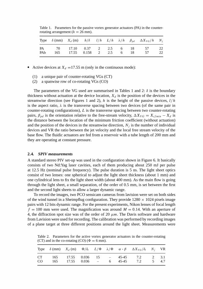
Table 1. Parameters for the passive vortex generator actuators (PA) in the counter-rotating arrangement (h = 26 mm).
Type δ (mm) Xd (m) h/δ l/h L/h λ/h βpd �XV G/h Nj
PA 70 17.10 0.37 2 2.5 6 18 57 22PAb 165 17.55 0.158 2 2.5 6 18 57 22
� Active devices at Xd =17.55 m (only in the continuous mode):
(1) a unique pair of counter-rotating VGs (CT)(2) a spanwise row of co-rotating VGs (CO)
The parameters of the VG used are summarised in Tables 1 and 2: δ is the boundarythickness without actuation at the device location, Xd is the position of the devices in thestreamwise direction (see Figures 1 and 2), h is the height of the passive devices, l/h
is the aspect ratio, λ is the transverse spacing between two devices (of the same pair incounter-rotating configurations), L is the transverse spacing between two counter-rotatingpairs, βpd is the orientation relative to the free-stream velocity, �XV G = Xcf min − Xd isthe distance between the location of the minimum friction coefficient (without actuation)and the position of the devices in the streamwise direction, Nj is the number of individualdevices and VR the ratio between the jet velocity and the local free stream velocity of thebase flow. The fluidic actuators are fed from a reservoir with a tube length of 200 mm andthey are operating at constant pressure.
2.4. SPIV measurements
A standard stereo PIV set-up was used in the configuration shown in Figure 6. It basicallyconsists of two Nd:Yag laser cavities, each of them producing about 250 mJ per pulseat 12.5 Hz (nominal pulse frequency). The pulse duration is 5 ns. The light sheet opticsconsist of two lenses: one spherical to adjust the light sheet thickness (about 1 mm) andone cylindrical lens to fix the light sheet width (about 400 mm). As the main flow is goingthrough the light sheet, a small separation, of the order of 0.5 mm, is set between the firstand the second light sheets to allow a larger dynamic range.
To record the images, two PCO sensicam cameras from lavision were set on both sidesof the wind tunnel in a Sheimpflug configuration. They provide 1280 × 1024 pixels imagepairs with 12 bits dynamic range. For the present experiments, Nikon lenses of focal lengthf = 100 mm were used. The magnification was around M = 0.14. With an aperture of4, the diffraction spot size was of the order of 20 µm. The Davis software and hardwarefrom Lavision were used for recording. The calibration was performed by recording imagesof a plane target at three different positions around the light sheet. Measurements were
Table 2. Parameters for the active vortex generator actuators in the counter-rotating(CT) and in the co-rotating (CO) (� = 6 mm).
Type δ (mm) Xd (m) �/δl L/� λ/� α - β �XV G/δl Nj VR
CT 165 17.55 0.036 15 – 45-45 7.2 2 3.1CO 165 17.55 0.036 – 6 45-45 7.2 5 4.7
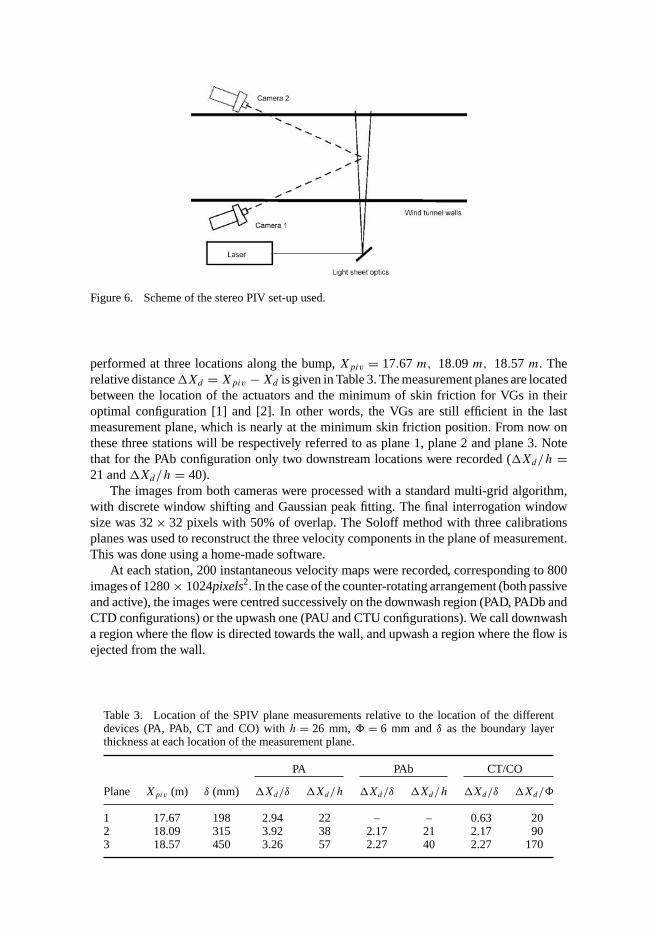
Figure 6. Scheme of the stereo PIV set-up used.
performed at three locations along the bump, Xpiv = 17.67 m, 18.09 m, 18.57 m. Therelative distance �Xd = Xpiv − Xd is given in Table 3. The measurement planes are locatedbetween the location of the actuators and the minimum of skin friction for VGs in theiroptimal configuration [1] and [2]. In other words, the VGs are still efficient in the lastmeasurement plane, which is nearly at the minimum skin friction position. From now onthese three stations will be respectively referred to as plane 1, plane 2 and plane 3. Notethat for the PAb configuration only two downstream locations were recorded (�Xd/h =21 and �Xd/h = 40).
The images from both cameras were processed with a standard multi-grid algorithm,with discrete window shifting and Gaussian peak fitting. The final interrogation windowsize was 32 × 32 pixels with 50% of overlap. The Soloff method with three calibrationsplanes was used to reconstruct the three velocity components in the plane of measurement.This was done using a home-made software.
At each station, 200 instantaneous velocity maps were recorded, corresponding to 800images of 1280 × 1024pixels2. In the case of the counter-rotating arrangement (both passiveand active), the images were centred successively on the downwash region (PAD, PADb andCTD configurations) or the upwash one (PAU and CTU configurations). We call downwasha region where the flow is directed towards the wall, and upwash a region where the flow isejected from the wall.
Table 3. Location of the SPIV plane measurements relative to the location of the differentdevices (PA, PAb, CT and CO) with h = 26 mm, � = 6 mm and δ as the boundary layerthickness at each location of the measurement plane.
PA PAb CT/CO
Plane Xpiv (m) δ (mm) �Xd/δ �Xd/h �Xd/δ �Xd/h �Xd/δ �Xd/�
1 17.67 198 2.94 22 – – 0.63 202 18.09 315 3.92 38 2.17 21 2.17 903 18.57 450 3.26 57 2.27 40 2.27 170
3. One point statistical analysis
3.1. Mean velocity
3.1.1. Mean velocity maps
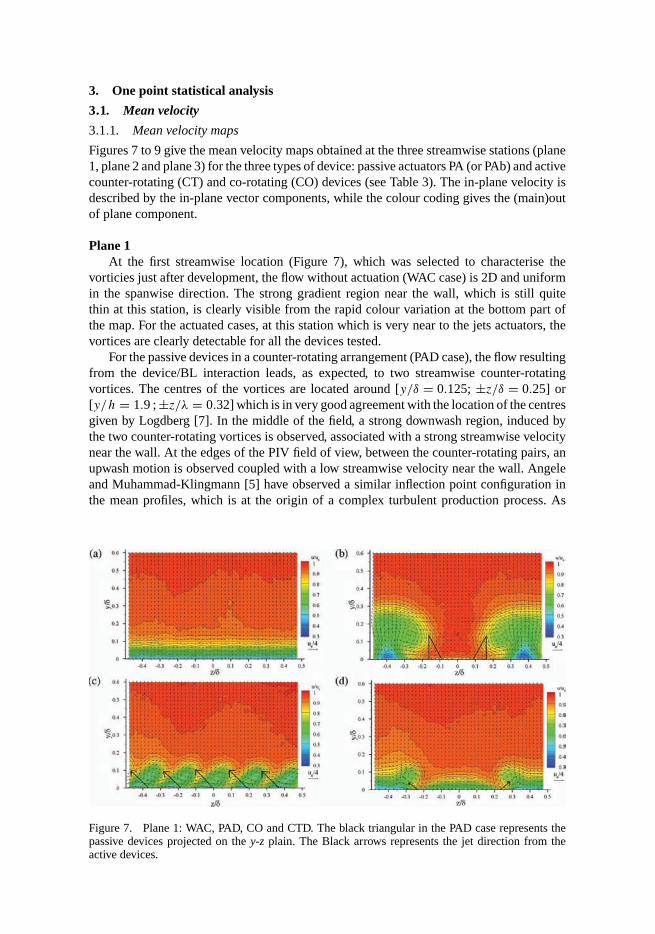
Figures 7 to 9 give the mean velocity maps obtained at the three streamwise stations (plane1, plane 2 and plane 3) for the three types of device: passive actuators PA (or PAb) and activecounter-rotating (CT) and co-rotating (CO) devices (see Table 3). The in-plane velocity isdescribed by the in-plane vector components, while the colour coding gives the (main)outof plane component.
Plane 1At the first streamwise location (Figure 7), which was selected to characterise the
vorticies just after development, the flow without actuation (WAC case) is 2D and uniformin the spanwise direction. The strong gradient region near the wall, which is still quitethin at this station, is clearly visible from the rapid colour variation at the bottom part ofthe map. For the actuated cases, at this station which is very near to the jets actuators, thevortices are clearly detectable for all the devices tested.
For the passive devices in a counter-rotating arrangement (PAD case), the flow resultingfrom the device/BL interaction leads, as expected, to two streamwise counter-rotatingvortices. The centres of the vortices are located around [y/δ = 0.125; ±z/δ = 0.25] or[y/h = 1.9 ; ±z/λ = 0.32] which is in very good agreement with the location of the centresgiven by Logdberg [7]. In the middle of the field, a strong downwash region, induced bythe two counter-rotating vortices is observed, associated with a strong streamwise velocitynear the wall. At the edges of the PIV field of view, between the counter-rotating pairs, anupwash motion is observed coupled with a low streamwise velocity near the wall. Angeleand Muhammad-Klingmann [5] have observed a similar inflection point configuration inthe mean profiles, which is at the origin of a complex turbulent production process. As
Figure 7. Plane 1: WAC, PAD, CO and CTD. The black triangular in the PAD case represents thepassive devices projected on the y-z plain. The Black arrows represents the jet direction from theactive devices.
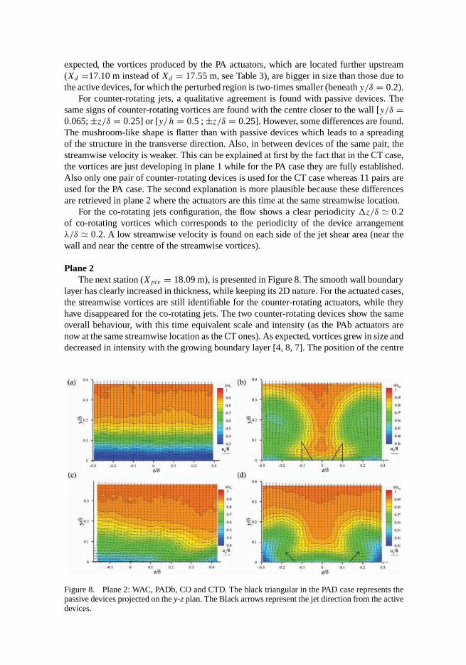
expected, the vortices produced by the PA actuators, which are located further upstream(Xd =17.10 m instead of Xd = 17.55 m, see Table 3), are bigger in size than those due tothe active devices, for which the perturbed region is two-times smaller (beneath y/δ = 0.2).
For counter-rotating jets, a qualitative agreement is found with passive devices. Thesame signs of counter-rotating vortices are found with the centre closer to the wall [y/δ =0.065; ±z/δ = 0.25] or [y/h = 0.5 ; ±z/δ = 0.25]. However, some differences are found.The mushroom-like shape is flatter than with passive devices which leads to a spreadingof the structure in the transverse direction. Also, in between devices of the same pair, thestreamwise velocity is weaker. This can be explained at first by the fact that in the CT case,the vortices are just developing in plane 1 while for the PA case they are fully established.Also only one pair of counter-rotating devices is used for the CT case whereas 11 pairs areused for the PA case. The second explanation is more plausible because these differencesare retrieved in plane 2 where the actuators are this time at the same streamwise location.
For the co-rotating jets configuration, the flow shows a clear periodicity �z/δ � 0.2of co-rotating vortices which corresponds to the periodicity of the device arrangementλ/δ � 0.2. A low streamwise velocity is found on each side of the jet shear area (near thewall and near the centre of the streamwise vortices).
Plane 2The next station (Xpiv = 18.09 m), is presented in Figure 8. The smooth wall boundary
layer has clearly increased in thickness, while keeping its 2D nature. For the actuated cases,the streamwise vortices are still identifiable for the counter-rotating actuators, while theyhave disappeared for the co-rotating jets. The two counter-rotating devices show the sameoverall behaviour, with this time equivalent scale and intensity (as the PAb actuators arenow at the same streamwise location as the CT ones). As expected, vortices grew in size anddecreased in intensity with the growing boundary layer [4, 8, 7]. The position of the centre
Figure 8. Plane 2: WAC, PADb, CO and CTD. The black triangular in the PAD case represents thepassive devices projected on the y-z plan. The Black arrows represent the jet direction from the activedevices.
of vortices is approximately (y/δ = 0.065; ±z/δ = 0.15] or [y/h = 0.79; ±z/λ = 0.30)for both counter rotating devices, which indicates that no significant lateral movement ofthe streamwise vortices is observed (±z/λ = 0.3 for the first two PIV plane locations). Onthe contrary, the vortices have moved away from the wall in the same ratio as the growthof the TBL without actuation (y/δ = 0.065 for the first two PIV plane locations). Thisindicates that the wall normal scaling for the mean vortex path is rather δ than h contrary toLogdberg et al. [7]. As at the previous station, the mushroom-like shape is flatter for activedevices with a weaker streamwise velocity in the very near wall region. Also, in betweendevices of the same pair, the streamwise velocity is weaker for the jet VGs.
For co-rotating devices, a very different behaviour is found, even if the field of view isobviously too small for this case, the wake of the VGs has turned into a region of momentumdownwash towards the wall, region which has moved to the right of the figure, due to selfinduction of the co-rotating vortical motion near the wall. Nevertheless, the BL momentumis improved in the whole region of observation.
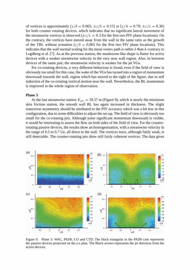
Plane 3At the last streamwise station Xpiv = 18.57 m (Figure 9), which is nearly the minimum
skin friction station, the smooth wall BL has again increased in thickness. The slighttransverse asymmetry should be attributed to the PIV accuracy which was a bit less in thisconfiguration, due to some difficulties to adjust the set-up. The field of view is obviously toosmall for the co-rotating jets. Although some significant momentum downwash is visible,it would be interesting to assess the flow on both sides of the field of view. For the counter-rotating passive devices, the results show an homogenisation, with a streamwise velocity inthe range of 0.5 to 0.7 Ue, all down to the wall. The vortices trace, although fairly weak, isstill detectable. The counter-rotating jets show still fairly coherent vortices. The data gives
Figure 9. Plane 3: WAC, PADb, CO and CTD. The black triangular in the PADb case representsthe passive devices projected on the y-z plan. The Black arrows represents the jet direction from theactive devices.
an evidence of alternations of low and high momentum regions near the wall, but with anincrease everywhere, as compared to the smooth wall.
SummaryFor an equivalent efficiency, around 200% of shear stress gain compared to the non-
actuated case (see Godard and Stanislas [2]), the PIV results in the three planes of ob-servation evidence little differences between PA and CT and high differences between CTand CO devices. The evolution for the streamwise vortices produced by counter-rotatingvortices are overall similar to the literature. The longitudinal evolution from co-rotatingconfiguration is subject to too few studies to be compared, although Lin [4] reports it to bemore efficient in 3D cross-flow configurations than in 2D configurations. In this study, theinitial individual vortices are observed to merge into a large single vortical region whichhas the ability to globally increase the momentum near the wall.
3.1.2. Mean profiles: comparison of actuator types
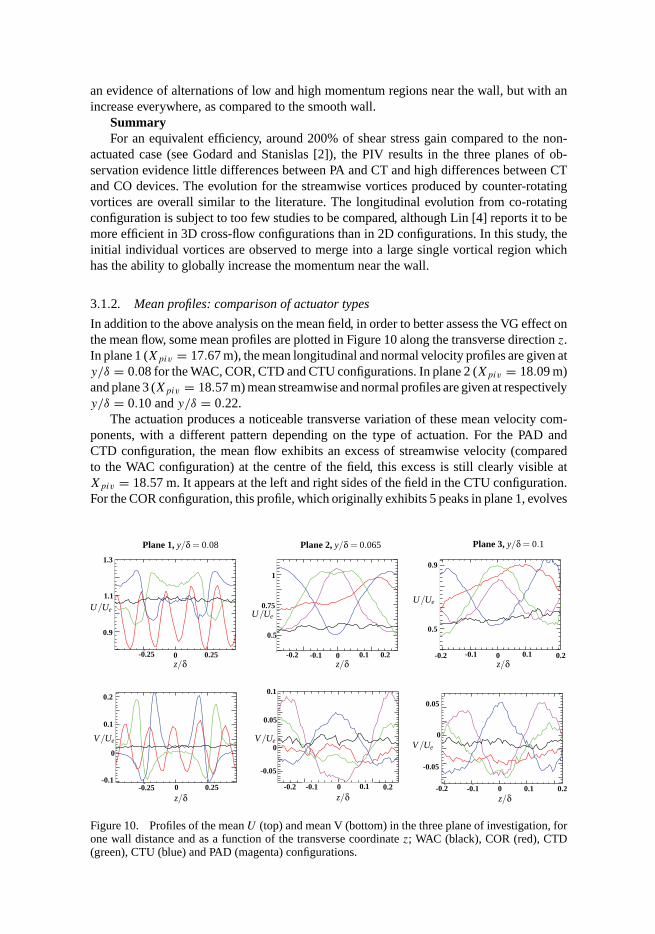
In addition to the above analysis on the mean field, in order to better assess the VG effect onthe mean flow, some mean profiles are plotted in Figure 10 along the transverse direction z.In plane 1 (Xpiv = 17.67 m), the mean longitudinal and normal velocity profiles are given aty/δ = 0.08 for the WAC, COR, CTD and CTU configurations. In plane 2 (Xpiv = 18.09 m)and plane 3 (Xpiv = 18.57 m) mean streamwise and normal profiles are given at respectivelyy/δ = 0.10 and y/δ = 0.22.
The actuation produces a noticeable transverse variation of these mean velocity com-ponents, with a different pattern depending on the type of actuation. For the PAD andCTD configuration, the mean flow exhibits an excess of streamwise velocity (comparedto the WAC configuration) at the centre of the field, this excess is still clearly visible atXpiv = 18.57 m. It appears at the left and right sides of the field in the CTU configuration.For the COR configuration, this profile, which originally exhibits 5 peaks in plane 1, evolves
0.25-0.25
0.250
-0.1 0.1
0.10-0.10
1
00
0
z/δ z/δ
z/δz/δz/δ
-0.25
z/δ
Plane 2, y/δ = 0.065Plane 1, y/δ = 0.08 Plane 3, y/δ = 0.1
V/UeV/Ue
-0.1-0.2 0.20.1 2.02.0-
0.2-0.2-0.1 0.1 0.2-0.2
0.1
0.05
-0.05
0.2
0.1
-0.1
0.9
0.50.50.9
0.05
-0.05
V/Ue
U/Ue
U/UeU/Ue 0.75
1.1
1.3
000
Figure 10. Profiles of the mean U (top) and mean V (bottom) in the three plane of investigation, forone wall distance and as a function of the transverse coordinate z; WAC (black), COR (red), CTD(green), CTU (blue) and PAD (magenta) configurations.
downstream such as a global increase of the streamwise velocity is noticeable in planes 2 and3 with a maximum around z/δ = 0.25. In all the actuated cases, a global acceleration of theflow is observed. It can also be noticed that a maximum of streamwise velocity correspondsto a negative minimum of the normal component and a minimum of streamwise velocitycorresponds to a positive maximum of V (except for the COR configuration in plane 3,where no extrema is clearly noticeable on the normal velocity profile). Actually, negativenormal velocity corresponds to a transport of high-speed fluid from the free-stream. On thecontrary, positive normal velocity corresponds to a transport of low-speed fluid outside theboundary layer. A clear difference in behaviour between co- and counter-rotating devicescan be noticed. For the COR, in plane 1 and at the chosen altitude, a momentum deficitappears on average compared to the WAC case. This is due to the fact that the vortices arecompactly staggered near the wall and leave little room between them for downwash. Inplanes 2 and 3, the individual vortices of plane 1 have merged together. The momentumbenefit is clearly visible and the wake of the actuating device has moved transversely by selfinduction. For the different counter-rotating configurations, the lifetime of the individualvortices is much longer and the momentum transfer is in evident agreement with the signand location of the different vortices. One solution to avoid the merging in the co-rotatingcase would be to increase the transverse spacing, but it has been shown by Godard andStanislas [1, 2] that this reduces the overall efficiency of the device.
3.2. Turbulent kinetic energy
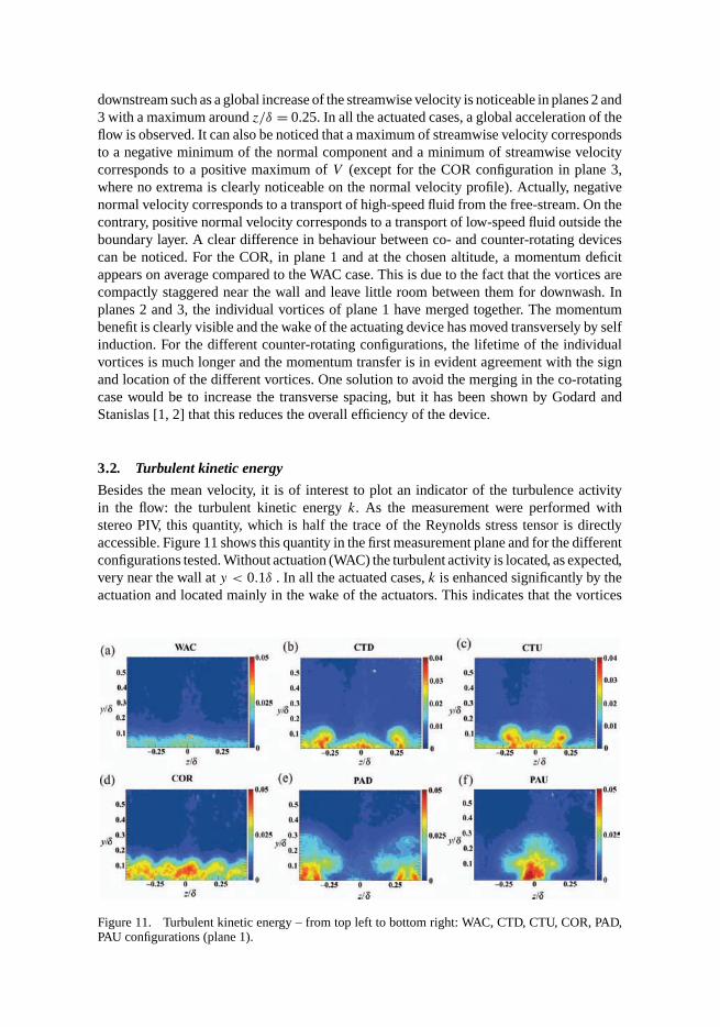
Besides the mean velocity, it is of interest to plot an indicator of the turbulence activityin the flow: the turbulent kinetic energy k. As the measurement were performed withstereo PIV, this quantity, which is half the trace of the Reynolds stress tensor is directlyaccessible. Figure 11 shows this quantity in the first measurement plane and for the differentconfigurations tested. Without actuation (WAC) the turbulent activity is located, as expected,very near the wall at y < 0.1δ . In all the actuated cases, k is enhanced significantly by theactuation and located mainly in the wake of the actuators. This indicates that the vortices
Figure 11. Turbulent kinetic energy – from top left to bottom right: WAC, CTD, CTU, COR, PAD,PAU configurations (plane 1).
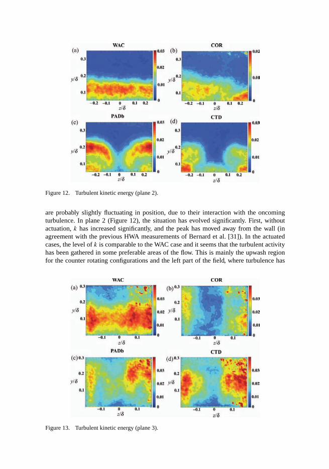
Figure 12. Turbulent kinetic energy (plane 2).
are probably slightly fluctuating in position, due to their interaction with the oncomingturbulence. In plane 2 (Figure 12), the situation has evolved significantly. First, withoutactuation, k has increased significantly, and the peak has moved away from the wall (inagreement with the previous HWA measurements of Bernard et al. [31]). In the actuatedcases, the level of k is comparable to the WAC case and it seems that the turbulent activityhas been gathered in some preferable areas of the flow. This is mainly the upwash regionfor the counter rotating configurations and the left part of the field, where turbulence has
Figure 13. Turbulent kinetic energy (plane 3).

been spread as compared to the WAC case, for the co-rotating configuration. In plane 3(Figure 13), which is far downstream (in the region of minimum wall shear stress) theturbulence peak is still intense. In the WAC case, it is wider and further away from the wall,in agreement with previous hot wire measurements [31]. The counter-rotating actuatorsclearly redistribute k at the top of the upwash regions. For the co-rotating case, the resultsare difficult to interpret.
As a conclusion, the actuators seem to generate turbulence in plane 1. This ‘apparent’turbulence is probably due to the fluctuation in position of the vortices, as it becomesrapidly comparable in intensity to the natural one (planes 2 and 3). The actuation seemsto redistribute spatially this turbulence. This is particularly evident for the counter-rotatingactuators.
4. Spatial correlations
Spatial correlation is classically used to reveal the underlying organisation of turbulentflows. In the present case, in order to asses the organising ability of the streamwise vortices,we have computed the two points spatial correlation of the velocity fields. The two pointspatial correlation co-efficients are defined as the temporal mean value of the followingrelation:
Rij (�x,−→dx, t) = 〈 �ui(�x, t). �uj (�x + −→
dx, t)〉〈 �ui(�x, t). �ui(�x, t)〉〈 �uj (�x + −→
dx, t). �uj (�x + −→dx, t)〉
. (1)
The vector �x is a two-component vector in the plane (y, z), and it represents the coordinatesof a fixed point,
−→dx represents the coordinates of the moving point, and t is the time. In
the present case, an ergodicity hypothesis is used: the average is not computed on timebut as an ensemble average on the number of PIV maps which are supposed completelyuncorrelated (this is true as the time separation between two maps is much larger than thetime scale of the Taylor macro scales of the flow).
In all the results presented below, the direction normal to the wall is considered asthe non-homogeneous direction. The transverse direction will sometimes be consideredhomogeneous. In this case, the correlation coefficients are averaged along the z direction,and the fixed point is then defined by its single wall normal coordinate y.
4.1. Without actuation
First, the different spatial correlation coefficients in planes 2 and 3 in the configurationwithout actuation (referred to as WAC) were computed. In this particular case, the transversedirection z is considered as homogeneous. Figures 14 and 15 show these coefficients. Thealtitude of the fixed point is y/δ = 0.065 for plane 2 and y/δ = 0.010 for the plane 3.These altitudes correspond more or less to the centre of the vortices, when the actuatorsare in operation. As can be seen, the normal coefficients R22 and R33 are fairly localised,with an increase of the scales when going downstream. The wall normal velocity gradientis detectable in plane 2 on R22 as the correlation is computed here on the instantaneousvelocities and not on the fluctuations. The cross correlation coefficients R23 and R32 showa shape which has already been observed by Bernard et al. [31] and which is typical ofvortices normal to the PIV plane. Again, the size of these vortices increases downstream.
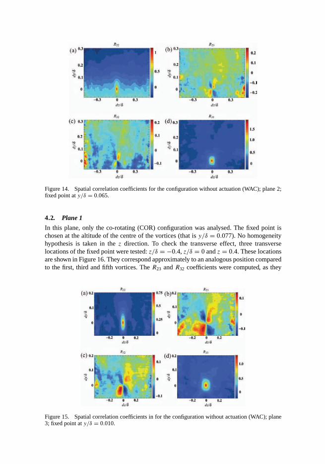
Figure 14. Spatial correlation coefficients for the configuration without actuation (WAC); plane 2;fixed point at y/δ = 0.065.
4.2. Plane 1
In this plane, only the co-rotating (COR) configuration was analysed. The fixed point ischosen at the altitude of the centre of the vortices (that is y/δ = 0.077). No homogeneityhypothesis is taken in the z direction. To check the transverse effect, three transverselocations of the fixed point were tested: z/δ = −0.4, z/δ = 0 and z = 0.4. These locationsare shown in Figure 16. They correspond approximately to an analogous position comparedto the first, third and fifth vortices. The R23 and R32 coefficients were computed, as they
Figure 15. Spatial correlation coefficients in for the configuration without actuation (WAC); plane3; fixed point at y/δ = 0.010.
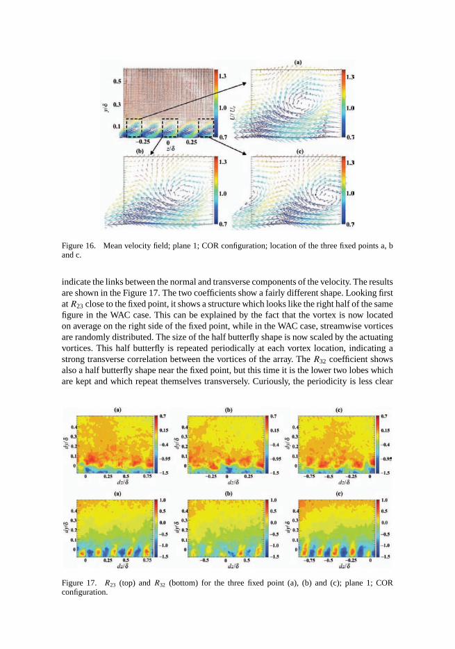
Figure 16. Mean velocity field; plane 1; COR configuration; location of the three fixed points a, band c.
indicate the links between the normal and transverse components of the velocity. The resultsare shown in the Figure 17. The two coefficients show a fairly different shape. Looking firstat R23 close to the fixed point, it shows a structure which looks like the right half of the samefigure in the WAC case. This can be explained by the fact that the vortex is now locatedon average on the right side of the fixed point, while in the WAC case, streamwise vorticesare randomly distributed. The size of the half butterfly shape is now scaled by the actuatingvortices. This half butterfly is repeated periodically at each vortex location, indicating astrong transverse correlation between the vortices of the array. The R32 coefficient showsalso a half butterfly shape near the fixed point, but this time it is the lower two lobes whichare kept and which repeat themselves transversely. Curiously, the periodicity is less clear
Figure 17. R23 (top) and R32 (bottom) for the three fixed point (a), (b) and (c); plane 1; CORconfiguration.
at point b, but this should be attributed to a lack of convergence as only 200 samples areavailable to compute the correlation coefficients when no homogeneity hypothesis is used.In fact a slightly better convergence could be achieved by averaging the three maps ofFigure 17.
4.3. Plane 2
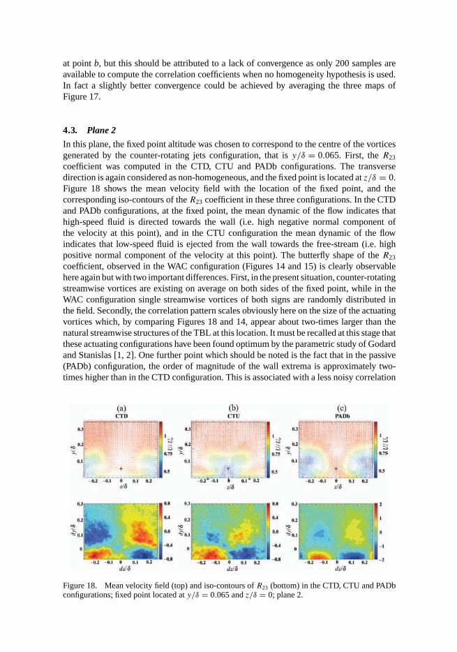
In this plane, the fixed point altitude was chosen to correspond to the centre of the vorticesgenerated by the counter-rotating jets configuration, that is y/δ = 0.065. First, the R23
coefficient was computed in the CTD, CTU and PADb configurations. The transversedirection is again considered as non-homogeneous, and the fixed point is located at z/δ = 0.Figure 18 shows the mean velocity field with the location of the fixed point, and thecorresponding iso-contours of the R23 coefficient in these three configurations. In the CTDand PADb configurations, at the fixed point, the mean dynamic of the flow indicates thathigh-speed fluid is directed towards the wall (i.e. high negative normal component ofthe velocity at this point), and in the CTU configuration the mean dynamic of the flowindicates that low-speed fluid is ejected from the wall towards the free-stream (i.e. highpositive normal component of the velocity at this point). The butterfly shape of the R23
coefficient, observed in the WAC configuration (Figures 14 and 15) is clearly observablehere again but with two important differences. First, in the present situation, counter-rotatingstreamwise vortices are existing on average on both sides of the fixed point, while in theWAC configuration single streamwise vortices of both signs are randomly distributed inthe field. Secondly, the correlation pattern scales obviously here on the size of the actuatingvortices which, by comparing Figures 18 and 14, appear about two-times larger than thenatural streamwise structures of the TBL at this location. It must be recalled at this stage thatthese actuating configurations have been found optimum by the parametric study of Godardand Stanislas [1, 2]. One further point which should be noted is the fact that in the passive(PADb) configuration, the order of magnitude of the wall extrema is approximately two-times higher than in the CTD configuration. This is associated with a less noisy correlation
Figure 18. Mean velocity field (top) and iso-contours of R23 (bottom) in the CTD, CTU and PADbconfigurations; fixed point located at y/δ = 0.065 and z/δ = 0; plane 2.
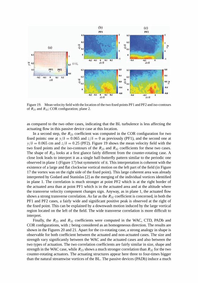
Figure 19. Mean velocity field with the location of the two fixed points PF1 and PF2 and iso-contoursof R23 and R32; COR configuration; plane 2.
as compared to the two other cases, indicating that the BL turbulence is less affecting theactuating flow in this passive device case at this location.
In a second step, the R23 coefficient was computed in the COR configuration for twofixed points: one at y/δ = 0.065 and z/δ = 0 as previously (PF1), and the second one aty/δ = 0.065 cm and z/δ = 0.25 (PF2). Figure 19 shows the mean velocity field with thetwo fixed points and the iso-contours of the R23 and R32 coefficients for these two cases.The shape of R23 looks at a first glance fairly different from the counter-rotating case. Aclose look leads to interpret it as a single half-butterfly pattern similar to the periodic oneobserved in plane 1 (Figure 17) but symmetric of it. This interpretation is coherent with theexistence of a large and flat clockwise vortical motion on the left part of the field (in Figure17 the vortex was on the right side of the fixed point). This large coherent area was alreadyinterpreted by Godard and Stanislas [2] as the merging of the individual vortices identifiedin plane 1. The correlation is much stronger at point PF2 which is at the right border ofthe actuated area than at point PF1 which is in the actuated area and at the altitude wherethe transverse velocity component changes sign. Anyway, as in plane 1, the actuated flowshows a strong transverse correlation. As far as the R32 coefficient is concerned, in both thePF1 and PF2 cases, a fairly wide and significant positive peak is observed at the right ofthe fixed point. This can be explained by a downwash motion induced by the large vorticalregion located on the left of the field. The wide transverse correlation is more difficult tointerpret.
Finally, the R23 and R32 coefficients were computed in the WAC, CTD, PADb andCOR configurations, with z being considered as an homogeneous direction. The results areshown in the Figures 20 and 21. Apart for the co-rotating case, a strong analogy in shape isobservable for both coefficient between the actuated and non-actuated cases. The size andstrength vary significantly between the WAC and the actuated cases and also between thetwo types of actuation. The two correlation coefficients are fairly similar in size, shape andstrength in the WAC case, while R23 shows a much stronger correlation than R32 for the twocounter-rotating actuators. The actuating structures appear here three to four-times biggerthan the natural streamwise vortices of the BL. The passive devices (PADb) induce a much
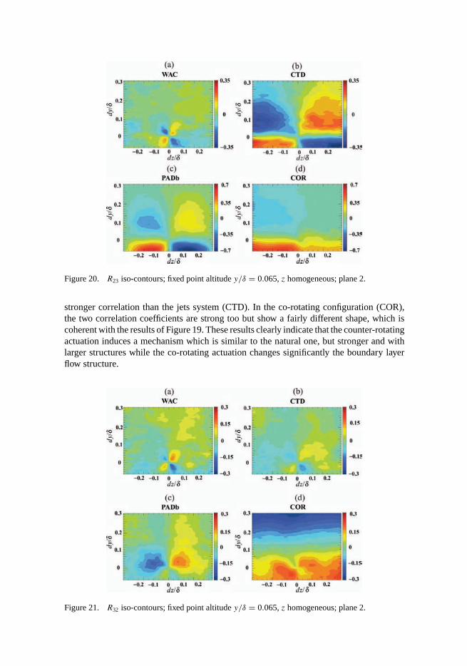
Figure 20. R23 iso-contours; fixed point altitude y/δ = 0.065, z homogeneous; plane 2.
stronger correlation than the jets system (CTD). In the co-rotating configuration (COR),the two correlation coefficients are strong too but show a fairly different shape, which iscoherent with the results of Figure 19. These results clearly indicate that the counter-rotatingactuation induces a mechanism which is similar to the natural one, but stronger and withlarger structures while the co-rotating actuation changes significantly the boundary layerflow structure.
Figure 21. R32 iso-contours; fixed point altitude y/δ = 0.065, z homogeneous; plane 2.
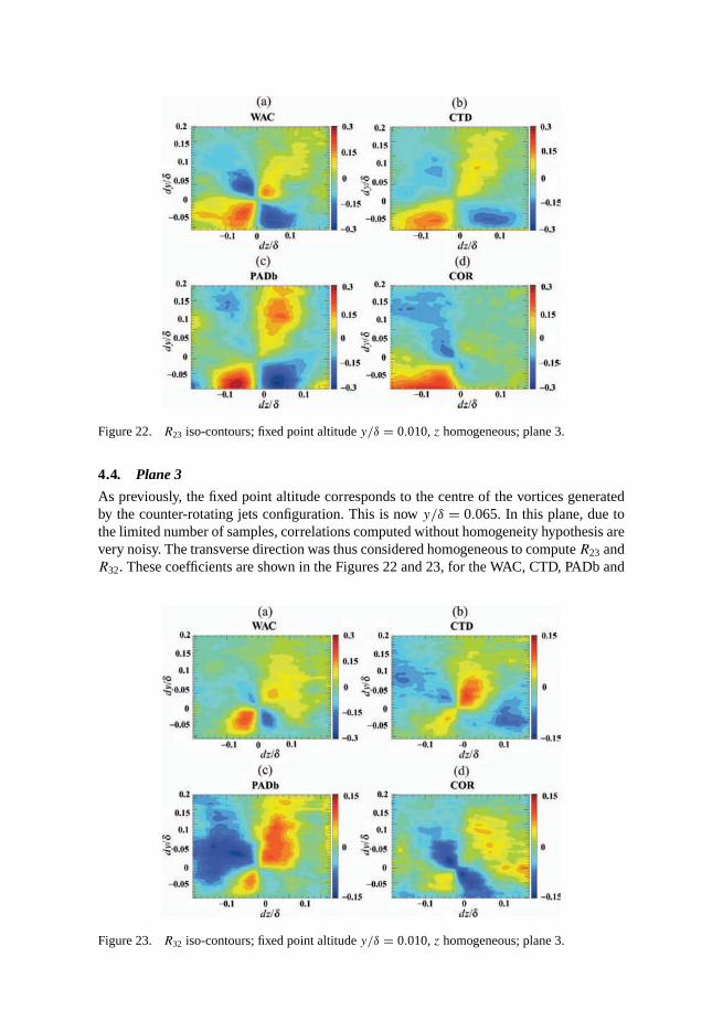
Figure 22. R23 iso-contours; fixed point altitude y/δ = 0.010, z homogeneous; plane 3.
4.4. Plane 3
As previously, the fixed point altitude corresponds to the centre of the vortices generatedby the counter-rotating jets configuration. This is now y/δ = 0.065. In this plane, due tothe limited number of samples, correlations computed without homogeneity hypothesis arevery noisy. The transverse direction was thus considered homogeneous to compute R23 andR32. These coefficients are shown in the Figures 22 and 23, for the WAC, CTD, PADb and
Figure 23. R32 iso-contours; fixed point altitude y/δ = 0.010, z homogeneous; plane 3.
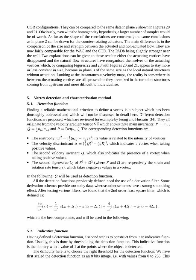
COR configurations. They can be compared to the same data in plane 2 shown in Figures 20and 21. Obviously, even with the homogeneity hypothesis, a larger number of samples wouldbe of worth. As far as the shape of the correlations are concerned, the same conclusionsas in plane 2 can be drawn for the counter-rotating actuators. The main difference is in thecomparison of the size and strength between the actuated and non-actuated flow. They arenow fairly comparable for the WAC and the CTD. The PADb being slightly stronger nearthe wall. Two explanations can be given to these results: either the actuating vortices havedisappeared and the natural flow structures have reorganised themselves or the actuatingvortices which, by comparing Figures 22 and 23 with Figures 20 and 21, appear to stay moreor less constant in size, become in plane 3 of the same size as the local natural structureswithout actuation. Looking at the instantaneous velocity maps, the reality is somewhere inbetween: the actuating vortices are still present but they are mixed in the turbulent structurescoming from upstream and more difficult to individualise.
5. Vortex detection and characterisation method
5.1. Detection function
Finding a reliable mathematical criterion to define a vortex is a subject which has beenthoroughly addressed and which will not be discussed in detail here. Different detectionfunctions are proposed, which are reviewed for example by Jeong and Hussain [34]. They alloriginate from the velocity gradient tensor ∇�u which shows three main invariants: P = ui,i ,Q = 1
2ui,juj,i and R = Det(ui,j ). The corresponding detection functions are:
� The enstrophy |ω|2 = | 12 (ui,j − uj,i)|2; its value is related to the intensity of vortices.
� The velocity discriminant � = ( 13Q)3 − ( 1
2R)2, which indicates a vortex when takingpositive values.
� The second velocity invariant Q, which also indicates the presence of a vortex whentaking positive values.
� The second eigenvalue λ2 of S2 + 2 (where S and are respectively the strain androtation rate tensors), which takes negatives values in a vortex.
In the following, Q will be used as detection function.All the detection functions previously defined need the use of a derivation filter. Some
derivation schemes provide too noisy data, whereas other schemes have a strong smoothingeffect. After testing various filters, we found that the 2nd order least square filter, which isdefined as:
∂u
∂x(xi) = 1
17[u(xi + �x) − u(xi − �x)] + 4
17[u(xi + 4�x) − u(xi − 4�x)],
which is the best compromise, and will be used in the following.
5.2. Indicative function
Having defined a detection function, a second step is to construct from it an indicative func-tion. Usually, this is done by thresholding the detection function. This indicative functionis then binary with a value of 1 at the points where the object is detected.
The difficulty here is to choose the right threshold for the detection function. We havefirst scaled the detection function as an 8 bits image, i.e. with values from 0 to 255. This
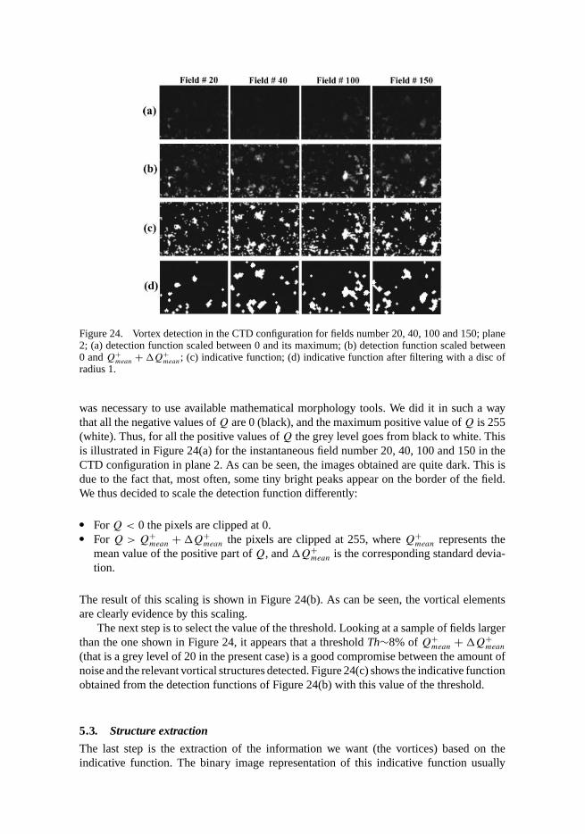
Figure 24. Vortex detection in the CTD configuration for fields number 20, 40, 100 and 150; plane2; (a) detection function scaled between 0 and its maximum; (b) detection function scaled between0 and Q+
mean + �Q+mean; (c) indicative function; (d) indicative function after filtering with a disc of
radius 1.
was necessary to use available mathematical morphology tools. We did it in such a waythat all the negative values of Q are 0 (black), and the maximum positive value of Q is 255(white). Thus, for all the positive values of Q the grey level goes from black to white. Thisis illustrated in Figure 24(a) for the instantaneous field number 20, 40, 100 and 150 in theCTD configuration in plane 2. As can be seen, the images obtained are quite dark. This isdue to the fact that, most often, some tiny bright peaks appear on the border of the field.We thus decided to scale the detection function differently:
� For Q < 0 the pixels are clipped at 0.� For Q > Q+
mean + �Q+mean the pixels are clipped at 255, where Q+
mean represents themean value of the positive part of Q, and �Q+
mean is the corresponding standard devia-tion.
The result of this scaling is shown in Figure 24(b). As can be seen, the vortical elementsare clearly evidence by this scaling.
The next step is to select the value of the threshold. Looking at a sample of fields largerthan the one shown in Figure 24, it appears that a threshold Th∼8% of Q+
mean + �Q+mean
(that is a grey level of 20 in the present case) is a good compromise between the amount ofnoise and the relevant vortical structures detected. Figure 24(c) shows the indicative functionobtained from the detection functions of Figure 24(b) with this value of the threshold.
5.3. Structure extraction
The last step is the extraction of the information we want (the vortices) based on theindicative function. The binary image representation of this indicative function usually
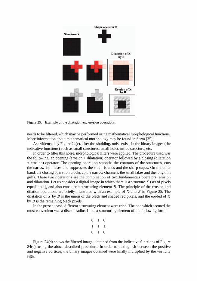
Figure 25. Example of the dilatation and erosion operations.
needs to be filtered, which may be performed using mathematical morphological functions.More information about mathematical morphology may be found in Serra [35].
As evidenced by Figure 24(c), after thresholding, noise exists in the binary images (theindicative functions) such as small structures, small holes inside structure, etc.
In order to filter this noise, morphological filters were applied. The procedure used wasthe following: an opening (erosion + dilatation) operator followed by a closing (dilatation+ erosion) operator. The opening operation smooths the contours of the structures, cutsthe narrow isthmuses and suppresses the small islands and the sharp capes. On the otherhand, the closing operation blocks up the narrow channels, the small lakes and the long thingulfs. These two operations are the combination of two fundamentals operators: erosionand dilatation. Let us consider a digital image in which there is a structure X (set of pixelsequals to 1), and also consider a structuring element B. The principle of the erosion anddilation operations are briefly illustrated with an example of X and B in Figure 25. Thedilatation of X by B is the union of the black and shaded red pixels, and the eroded of X
by B is the remaining black pixels.In the present case, different structuring element were tried. The one which seemed the
most convenient was a disc of radius 1, i.e. a structuring element of the following form:
0 1 0
1 1 1
0 1 0
.
Figure 24(d) shows the filtered image, obtained from the indicative functions of Figure24(c), using the above described procedure. In order to distinguish between the positiveand negative vortices, the binary images obtained were finally multiplied by the vorticitysign.
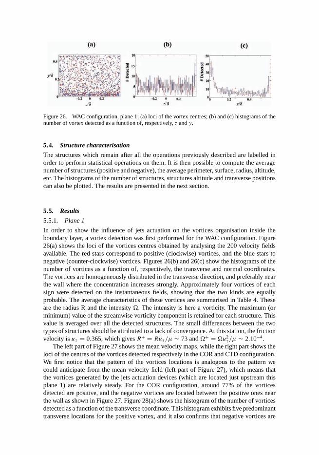
Figure 26. WAC configuration, plane 1; (a) loci of the vortex centres; (b) and (c) histograms of thenumber of vortex detected as a function of, respectively, z and y.
5.4. Structure characterisation
The structures which remain after all the operations previously described are labelled inorder to perform statistical operations on them. It is then possible to compute the averagenumber of structures (positive and negative), the average perimeter, surface, radius, altitude,etc. The histograms of the number of structures, structures altitude and transverse positionscan also be plotted. The results are presented in the next section.
5.5. Results
5.5.1. Plane 1
In order to show the influence of jets actuation on the vortices organisation inside theboundary layer, a vortex detection was first performed for the WAC configuration. Figure26(a) shows the loci of the vortices centres obtained by analysing the 200 velocity fieldsavailable. The red stars correspond to positive (clockwise) vortices, and the blue stars tonegative (counter-clockwise) vortices. Figures 26(b) and 26(c) show the histograms of thenumber of vortices as a function of, respectively, the transverse and normal coordinates.The vortices are homogeneously distributed in the transverse direction, and preferably nearthe wall where the concentration increases strongly. Approximately four vortices of eachsign were detected on the instantaneous fields, showing that the two kinds are equallyprobable. The average characteristics of these vortices are summarised in Table 4. Theseare the radius R and the intensity . The intensity is here a vorticity. The maximum (orminimum) value of the streamwise vorticity component is retained for each structure. Thisvalue is averaged over all the detected structures. The small differences between the twotypes of structures should be attributed to a lack of convergence. At this station, the frictionvelocity is uτ = 0.365, which gives R+ = Ruτ/µ ∼ 73 and + = u2
τ /µ ∼ 2.10−4.The left part of Figure 27 shows the mean velocity maps, while the right part shows the
loci of the centres of the vortices detected respectively in the COR and CTD configuration.We first notice that the pattern of the vortices locations is analogous to the pattern wecould anticipate from the mean velocity field (left part of Figure 27), which means thatthe vortices generated by the jets actuation devices (which are located just upstream thisplane 1) are relatively steady. For the COR configuration, around 77% of the vorticesdetected are positive, and the negative vortices are located between the positive ones nearthe wall as shown in Figure 27. Figure 28(a) shows the histogram of the number of vorticesdetected as a function of the transverse coordinate. This histogram exhibits five predominanttransverse locations for the positive vortex, and it also confirms that negative vortices are
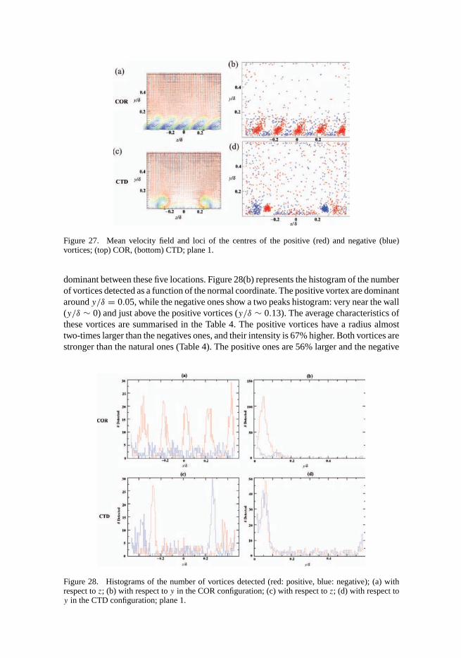
Figure 27. Mean velocity field and loci of the centres of the positive (red) and negative (blue)vortices; (top) COR, (bottom) CTD; plane 1.
dominant between these five locations. Figure 28(b) represents the histogram of the numberof vortices detected as a function of the normal coordinate. The positive vortex are dominantaround y/δ = 0.05, while the negative ones show a two peaks histogram: very near the wall(y/δ ∼ 0) and just above the positive vortices (y/δ ∼ 0.13). The average characteristics ofthese vortices are summarised in the Table 4. The positive vortices have a radius almosttwo-times larger than the negatives ones, and their intensity is 67% higher. Both vortices arestronger than the natural ones (Table 4). The positive ones are 56% larger and the negative
Figure 28. Histograms of the number of vortices detected (red: positive, blue: negative); (a) withrespect to z; (b) with respect to y in the COR configuration; (c) with respect to z; (d) with respect toy in the CTD configuration; plane 1.
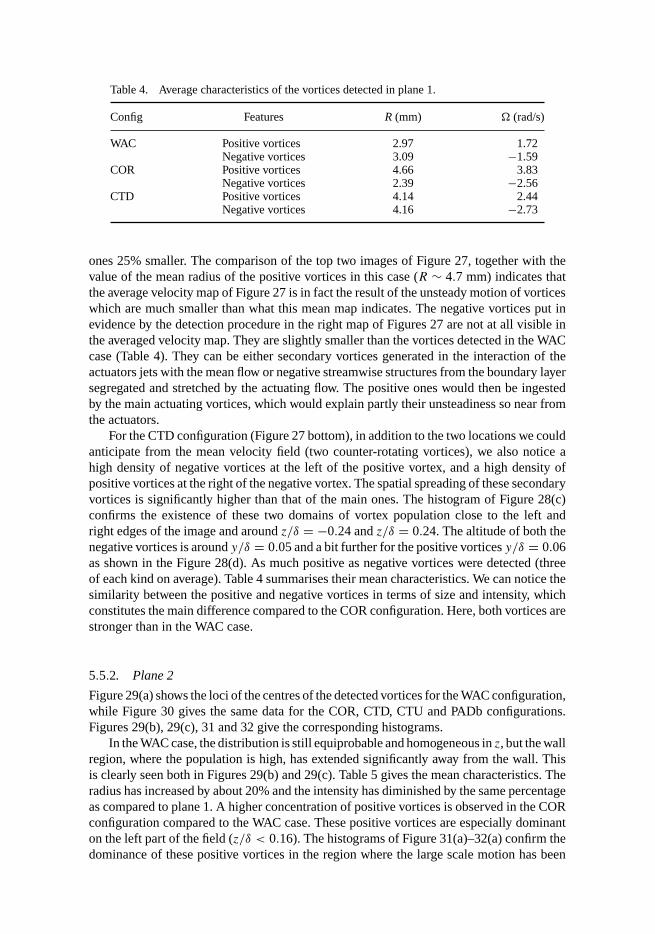
Table 4. Average characteristics of the vortices detected in plane 1.
Config Features R (mm) (rad/s)
WAC Positive vortices 2.97 1.72Negative vortices 3.09 −1.59
COR Positive vortices 4.66 3.83Negative vortices 2.39 −2.56
CTD Positive vortices 4.14 2.44Negative vortices 4.16 −2.73
ones 25% smaller. The comparison of the top two images of Figure 27, together with thevalue of the mean radius of the positive vortices in this case (R ∼ 4.7 mm) indicates thatthe average velocity map of Figure 27 is in fact the result of the unsteady motion of vorticeswhich are much smaller than what this mean map indicates. The negative vortices put inevidence by the detection procedure in the right map of Figures 27 are not at all visible inthe averaged velocity map. They are slightly smaller than the vortices detected in the WACcase (Table 4). They can be either secondary vortices generated in the interaction of theactuators jets with the mean flow or negative streamwise structures from the boundary layersegregated and stretched by the actuating flow. The positive ones would then be ingestedby the main actuating vortices, which would explain partly their unsteadiness so near fromthe actuators.
For the CTD configuration (Figure 27 bottom), in addition to the two locations we couldanticipate from the mean velocity field (two counter-rotating vortices), we also notice ahigh density of negative vortices at the left of the positive vortex, and a high density ofpositive vortices at the right of the negative vortex. The spatial spreading of these secondaryvortices is significantly higher than that of the main ones. The histogram of Figure 28(c)confirms the existence of these two domains of vortex population close to the left andright edges of the image and around z/δ = −0.24 and z/δ = 0.24. The altitude of both thenegative vortices is around y/δ = 0.05 and a bit further for the positive vortices y/δ = 0.06as shown in the Figure 28(d). As much positive as negative vortices were detected (threeof each kind on average). Table 4 summarises their mean characteristics. We can notice thesimilarity between the positive and negative vortices in terms of size and intensity, whichconstitutes the main difference compared to the COR configuration. Here, both vortices arestronger than in the WAC case.
5.5.2. Plane 2
Figure 29(a) shows the loci of the centres of the detected vortices for the WAC configuration,while Figure 30 gives the same data for the COR, CTD, CTU and PADb configurations.Figures 29(b), 29(c), 31 and 32 give the corresponding histograms.
In the WAC case, the distribution is still equiprobable and homogeneous in z, but the wallregion, where the population is high, has extended significantly away from the wall. Thisis clearly seen both in Figures 29(b) and 29(c). Table 5 gives the mean characteristics. Theradius has increased by about 20% and the intensity has diminished by the same percentageas compared to plane 1. A higher concentration of positive vortices is observed in the CORconfiguration compared to the WAC case. These positive vortices are especially dominanton the left part of the field (z/δ < 0.16). The histograms of Figure 31(a)–32(a) confirm thedominance of these positive vortices in the region where the large scale motion has been
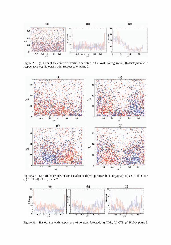
Figure 29. (a) Loci of the centres of vortices detected in the WAC configuration; (b) histogram withrespect to z; (c) histogram with respect to y; plane 2.
Figure 30. Loci of the centres of vortices detected (red: positive, blue: negative); (a) COR, (b) CTD,(c) CTU, (d) PADb; plane 2.
Figure 31. Histograms with respect to z of vortices detected; (a) COR, (b) CTD (c) PADb; plane 2.

Figure 32. Histograms with respect to y of vortices detected; (a) COR, (b) CTD, (c) PADb; plane 2.
previously identified (Figure 19). In the COR configuration, we detected 75% more positivethan negative vortices (about 7 positives and 4 negatives on each instantaneous field). Table5 gives the mean characteristics of these vortices. Their intensity has significantly decreasedas compared to plane 1 and is now comparable, for both signs, to the WAC case in plane2. The positive vortices have decreased in size, while the negative ones have increased,compared to plane 1, but a difference still exists in plane 2 between both signs.
In the CTD configuration (Figure 30(b)), a concentration of positive vortices can bedistinguished around z/δ = −0.18 , and of negative vortices around z/δ = 0.18 (see Figure30(b) and Figures 31(b)–32(b)). A deficit of vortices is observed at the centre of theimage, which corresponds to the downwash zone. Vortices of opposite sign gather nearthe wall and on each side of the origin and to a less extent, outside and above the mainvortex (z/δ = ±0.24, y/δ = 0.16). In the CTU configuration, the opposite behaviour isobtained, with a concentration of vortices at the centre of the field (positive vortices aroundz/δ = −0.13 and negative vortices around z/δ = 0.13), which is an upwash zone, and adeficit of vortices at the left and right edges (downwash zones). The mean characteristicsare given in Table 5 for the CTD and for the CTU. First, the agreement appears fairly goodbetween the two configurations which correspond to the same flow at different transverselocation. The vortices are slightly smaller than in plane 1 (about 10% on the radius)and comparable to the positive vortices of the COR case. Their intensity has decreasedsignificantly (by about 50%) and is now comparable to that of the WAC and COR vortices.
The PADb configuration is quite similar to the CTD one (see Figures 30(d) and 31(c)–32(c)). However, it can be noticed that the transverse location of the positive vorticesconcentration is around z/δ = −0.16 and around z/δ = 0.16 for the negative vortices.Consequently, the downwash zone between these two concentrations is narrower than in the
Table 5. Average characteristics of the vortices detected in plane 2.
Config Features R (mm) (rad/s)
WAC Positive vortices 3.55 1.35Negative vortices 3.54 −1.39
COR Positive vortices 3.90 1.32Negative vortices 3.247 −1.32
CTD Positive vortices 3.79 1.48Negative vortices 3.82 −1.45
CTU Positive vortices 3.84 1.33Negative vortices 3.83 −1.33
PADb Positive vortices 4.048 1.47Negative vortices 4.22 −1.60
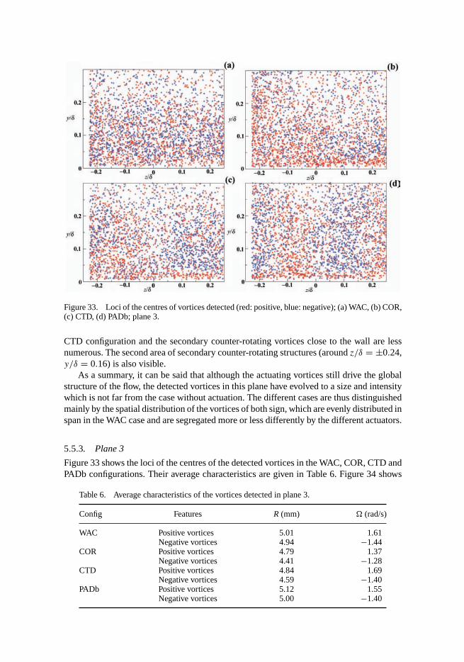
Figure 33. Loci of the centres of vortices detected (red: positive, blue: negative); (a) WAC, (b) COR,(c) CTD, (d) PADb; plane 3.
CTD configuration and the secondary counter-rotating vortices close to the wall are lessnumerous. The second area of secondary counter-rotating structures (around z/δ = ±0.24,y/δ = 0.16) is also visible.
As a summary, it can be said that although the actuating vortices still drive the globalstructure of the flow, the detected vortices in this plane have evolved to a size and intensitywhich is not far from the case without actuation. The different cases are thus distinguishedmainly by the spatial distribution of the vortices of both sign, which are evenly distributed inspan in the WAC case and are segregated more or less differently by the different actuators.
5.5.3. Plane 3
Figure 33 shows the loci of the centres of the detected vortices in the WAC, COR, CTD andPADb configurations. Their average characteristics are given in Table 6. Figure 34 shows
Table 6. Average characteristics of the vortices detected in plane 3.
Config Features R (mm) (rad/s)
WAC Positive vortices 5.01 1.61Negative vortices 4.94 −1.44
COR Positive vortices 4.79 1.37Negative vortices 4.41 −1.28
CTD Positive vortices 4.84 1.69Negative vortices 4.59 −1.40
PADb Positive vortices 5.12 1.55Negative vortices 5.00 −1.40
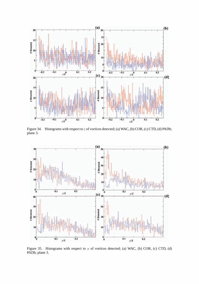
Figure 34. Histograms with respect to z of vortices detected; (a) WAC, (b) COR, (c) CTD, (d) PADb;plane 3.
Figure 35. Histograms with respect to y of vortices detected; (a) WAC, (b) COR, (c) CTD, (d)PADb; plane 3.
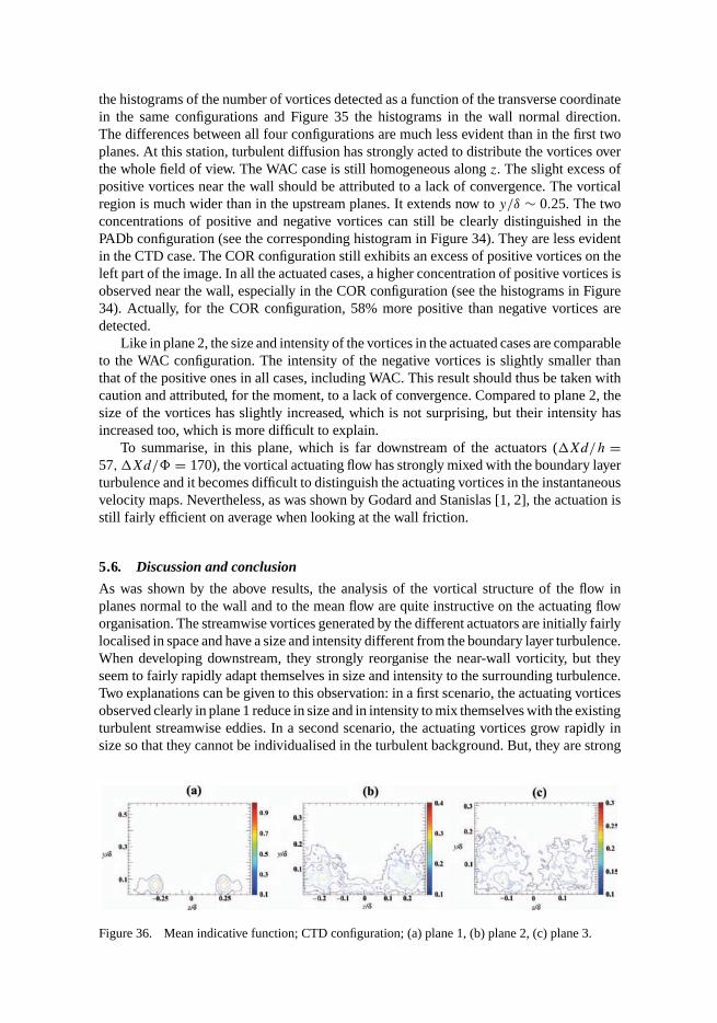
the histograms of the number of vortices detected as a function of the transverse coordinatein the same configurations and Figure 35 the histograms in the wall normal direction.The differences between all four configurations are much less evident than in the first twoplanes. At this station, turbulent diffusion has strongly acted to distribute the vortices overthe whole field of view. The WAC case is still homogeneous along z. The slight excess ofpositive vortices near the wall should be attributed to a lack of convergence. The vorticalregion is much wider than in the upstream planes. It extends now to y/δ ∼ 0.25. The twoconcentrations of positive and negative vortices can still be clearly distinguished in thePADb configuration (see the corresponding histogram in Figure 34). They are less evidentin the CTD case. The COR configuration still exhibits an excess of positive vortices on theleft part of the image. In all the actuated cases, a higher concentration of positive vortices isobserved near the wall, especially in the COR configuration (see the histograms in Figure34). Actually, for the COR configuration, 58% more positive than negative vortices aredetected.
Like in plane 2, the size and intensity of the vortices in the actuated cases are comparableto the WAC configuration. The intensity of the negative vortices is slightly smaller thanthat of the positive ones in all cases, including WAC. This result should thus be taken withcaution and attributed, for the moment, to a lack of convergence. Compared to plane 2, thesize of the vortices has slightly increased, which is not surprising, but their intensity hasincreased too, which is more difficult to explain.
To summarise, in this plane, which is far downstream of the actuators (�Xd/h =57,�Xd/� = 170), the vortical actuating flow has strongly mixed with the boundary layerturbulence and it becomes difficult to distinguish the actuating vortices in the instantaneousvelocity maps. Nevertheless, as was shown by Godard and Stanislas [1, 2], the actuation isstill fairly efficient on average when looking at the wall friction.
5.6. Discussion and conclusion
As was shown by the above results, the analysis of the vortical structure of the flow inplanes normal to the wall and to the mean flow are quite instructive on the actuating floworganisation. The streamwise vortices generated by the different actuators are initially fairlylocalised in space and have a size and intensity different from the boundary layer turbulence.When developing downstream, they strongly reorganise the near-wall vorticity, but theyseem to fairly rapidly adapt themselves in size and intensity to the surrounding turbulence.Two explanations can be given to this observation: in a first scenario, the actuating vorticesobserved clearly in plane 1 reduce in size and in intensity to mix themselves with the existingturbulent streamwise eddies. In a second scenario, the actuating vortices grow rapidly insize so that they cannot be individualised in the turbulent background. But, they are strong
Figure 36. Mean indicative function; CTD configuration; (a) plane 1, (b) plane 2, (c) plane 3.
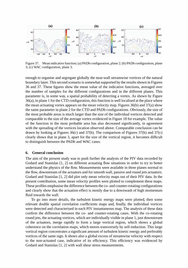
Figure 37. Mean indicative function; (a) PADb configuration, plane 2; (b) PADb configuration, plane3; (c) WAC configuration, plane 3.
enough to organise and segregate globally the near-wall streamwise vortices of the naturalboundary layer. This second scenario is somewhat supported by the results shown in Figures36 and 37. These figures show the mean value of the indicative functions, averaged overthe number of samples for the different configurations and in the different planes. Thisparameter is, in some way, a spatial probability of detecting a vortex. As shown by Figure36(a), in plane 1 for the CTD configuration, this function is well localised at the place wherethe mean actuating vortex appears on the mean velocity map. Figures 36(b) and 37(a) showthe same parameter in plane 2 for the CTD and PADb configurations. Obviously, the size ofthe most probable areas is much larger than the size of the individual vortices detected andcomparable to the size of the average vortex evidenced in Figure 18 for example. The valueof the function in the most probable area has also decreased significantly, in agreementwith the spreading of the vortices location observed above. Comparable conclusion can bedrawn by looking at Figures 36(c) and 37(b). The comparison of Figures 37(b) and 37(c)clearly shows that in plane 3, apart for the size of the vortical region, it becomes difficultto distinguish between the PADb and WAC cases.
6. General conclusion
The aim of the present study was to push further the analysis of the PIV data recorded byGodard and Stanislas [1, 2] on different actuating flow situations in order to try to betterunderstand the physics of the flow. Measurements were available in three planes normal tothe flow, downstream of the actuators and for smooth wall, passive and round jets actuators.Godard and Stanislas [1, 2] did plot only mean velocity maps out of their PIV data. In thepresent contribution, some mean velocity profiles were plotted to complement these maps.These profiles emphasise the difference between the co- and counter-rotating configurationsand clearly show that the actuation effect is mostly due to a downwash of high momentumfluid towards the wall.
To go into more details, the turbulent kinetic energy maps were plotted, then somerelevant double spatial correlation coefficients maps and, finally, the individual vorticeswere detected and characterised in each PIV instantaneous map. The analysis of these dataconfirm the difference between the co- and counter-rotating cases. With the co-rotatinground jets, the actuating vortices, which are individually visible in plane 1, just downstreamof the actuators, merge rapidly to form a large vortical region, which shows a globalcoherence on the correlation maps, which moves transversely by self-induction. This largevortical region concentrates a significant amount of turbulent kinetic energy and preferablyvortices of the same sign. It shows also a global excess of streamwise velocity with respectto the non-actuated case, indicative of its efficiency. This efficiency was evidenced byGodard and Stanislas [1, 2] with wall shear stress measurements.
The counter-rotating actuators (both passive and round jets) generate stable counter-rotating streamwise vortices which stay coherent and individualised far downstream. Thesevortices are much stronger than the natural boundary layer vortices in plane 1 but theyappear to progressively grow in size, reduce in intensity and mix themselves in the BLturbulence. They appear to segregate spatially this turbulence, concentrating the turbulentkinetic energy in the upwash regions. They also segregate the BL streamwise vortices,based on their sign, gathering them in different regions in space.
From the evolution observed in the three measurement planes, it can be expected thatthese actuating vortices progressively disappear downstream, but this may take a fairly longdistance.
AcknowledgementsThe research reported here was undertaken as part of the AEROMEMS II project (Advanced Aero-dynamic Flow Control Using MEMS, Contract No G4RD-CT-2002-00748). The AEROMEMS IIproject was a collaboration between BAE SYSTEMS, Dassault, Airbus Deutschland GmbH, EADS-Military, Snecma, ONERA, DLR, LPMO, Manchester University, LML, Warwick University, TUB,Cranfield University, NTUA, and Auxitrol. The project was funded by the European Union and theproject partners. Part of the work was also performed in the frame of CISIT.
References[1] G. Godard and M. Stanislas, Control of a decelerating boundary layer. Part 1: Optimization of
passive vortex generators, Aerosp. Sci. Technol. 10(3) (2006), pp. 181–191.[2] G. Godard and M. Stanislas, Control of a decelerating boundary layer. Part 3: Optimization of
round jets vortex generators, Aerosp. Sci. Technol. 10(6) (2006), pp. 455–464.[3] M. Gad el Hak, Flow Control: Passive, Active and Reactive Flow Management, Cambridge
University Press, Cambridge, 2000.[4] J.C. Lin, Review of research on low-profil vortex generators to control boundary layer separa-
tion, Prog. Aerosp. Sci. 38 (2002), pp. 389–420.[5] K.P. Angele and B. Muhammad-Klingmann, The effect of streamwise vortices on the turbulence
structure of a separating boundary layer, Eur. J. Mech. B/Fluids 24 (2005), pp. 539–554.[6] D. You et al., Large-eddy simulations of longitudinal vortices embedded in a turbulent boundary
layer, AIAA 44(12) (2006), pp. 3032–3039.[7] O. Logdberg, J.H.M. Fransson, and P.H. Alfredsson, Streamwise evolution of longitudinal
vortices in a turbulent boundary layer, J. Fluid Mech. 623 (2009), pp. 27–58.[8] C.P. Tilmann et al., Characterization of pulsed vortex generator jets for active flow control,
RTO AVT Symposium on “Active Control Technology for Enhanced Performance Opera-tional Capabilities of Military Aircraft, Land Vehicles and Sea Vehicles,” Germany, May 8–11,2000.
[9] G. Schubauer and W. Spangenberg, Forced mixing in boundary layers, J. Fluid Mech. 8 (1960),pp. 10–32.
[10] I.M.M.A. Shabaka, R.D. Mehta, and P. Bradshaw, Longitudinal vortices imbedded in turbulentboundary layers, J. Fluid Mech. 155 (1985), pp. 37–57.
[11] R.D. Mehta and P. Bradshaw, Longitudinal vortices imbedded in turbulent boundary layers.Part 2: Vortex pair with “common flow” upwards, J. Fluid Mech. 188 (1988), pp. 529–546.
[12] J.K. Eaton and W.R. Pauley, Experimental study of the development of longitudinal vortex pairsembedded in a turbulent boundary layer, AIAA J. 26(7) (1988), pp. 816–823.
[13] D.M. Rao and T.T. Kariya, Boundary-layer submerged vortex generators for separation control– an exploratory study, Space Programs Technol. 26(7) (1988), pp. 816–823.
[14] O. Logdberg, Turbulent boundary layer separation and control, Ph.D. thesis, KTH Engineeringscience, Stockholm, Sweden, 2008.
[15] A. Glezer and M. Amitay, Synthetic jets, Annu. Rev. Fluid Mech. 34 (2002), pp. 503–529.[16] K.L. Kudar and K.L. Carpenter, Numerical investigation and feasibility study of a pzt-driven
micro-valve pulsed-jet actuator, Flow Turbul. Combust. 78(3/4) (2007), pp. 223–254.
[17] C. Davies, A.A. Lockerby, and P.W. Carpenter, Is helmoltz resonnace a problem for micro-jetactuators? Flow Turbul. Combust. 78 (2007), pp. 205–222.
[18] J. Ortmanns and C.J. Kaehler, Investigation of pulsed actuators for active flow control usingphase locked stereoscopic particle image velocimetry, Twelfth International Symposium onApplications of Laser Techniques to Fluid Mechanics, Lisboa, Portugal, July 12–14, 2004.
[19] J. Kostas, J.M. Foucaut, and M. Stanislas, The flow structure produced by pulsed-jet vortexgenerators in a turbulent boundary layer in an adverse pressure gradient [Special issue onair-jet actuators and their use for flow control], Flow Turbul. Combust. 78 (2007), pp. 331–363.
[20] D. Greenblatt and I.J. Wygnansky, The control of flow separation by periodic excitation, Prog.Aerosp. Sci. 36 (2000), pp. 487–545.
[21] G. Raman et al., Development of high bandwidth powered resonance tube actuators withfeedback control, J. Sound Vib. 269 (2004), pp. 1031–1062.
[22] D.A. Compton and J.P. Johnston, Streamwise votex production by pitched and skewed jets in aturbulent boundary layer, AIAA J. 30(3) (1992), pp. 640–647.
[23] Z.U. Khan and J.P. Johnston, On vortex generating jets, Int. J. Heat Fluid Flow 21 (2000), pp.506–511.
[24] S.D. Peterson and M.W. Plesniak, Evolution of jets emanating from short holes into crossflow,J. Fluid Mech. 503 (2004), pp. 57–91.
[25] C. Warsop et al., Pulsed air-jet actuators for separation control, Flow Turbul. Combust. 78(2007), pp. 255–281.
[26] G.V. Selby, Control of low-speed turbulent separated flow using jet vortex generators, Exp.Fluids 12(6) (1992), pp. 394–400.
[27] C. Braud et al., Analysis and modelling of a fluidic actuator, ASME Summer Heat TransferConference, Jacksonville, USA, August 10–14, 2008.
[28] J. Ortmanns, M. Bitter, and C. Kaehler, Dynamic vortex structures for flow-control applications,Exp. Fluids 44 (2008), pp. 397–408.
[29] A. Bernard et al., Identification and assessment of flow actuation and control strategies, Tech.Rep. FREP/CN18/MS001101, LML UMR 8107, Lille, France, 2000.
[30] J. Carlier and M. Stanislas, Experimental study of eddy structures in a turbulent boundary layerusing particule image velocimetry, J. Fluid Mech. 535(36) (2005), pp. 143–188.
[31] A. Bernard et al., Decelerating boudary layer: A new scaling and mixing length model, AIAAJ. 41(2) (2003), pp. 248–255.
[32] G. Godard, J.M. Foucaut, and M. Stanislas, Control of a decelerating boundary layer. Part 2:Optimization of slotted jets vortex generators, Aerosp. Sci. Technol. 10(5) (2006), pp. 394–400.
[33] G. Godard et al., Optimization of passive and active vortex generators for boundary layercontrol, Tech. Rep. AEROMEMSII/TR/LML/1.1/GG040415-1, LML UMR CNRS 8107, Lille,France, April 15, 2004.
[34] J. Jeong and F. Hussain, On the identification of a vortex, J. Fluid Mech. 285 (1995), pp. 69–94.[35] J. Serra, Image Analysis and Mathematical Morphology, Academic Press, London, 1982.


![ORIE 6326: Convex Optimization [2ex] Operators · ORIE 6326: Convex Optimization Operators Professor Udell Operations Research and Information Engineering Cornell May 15, 2017 1/47](https://img.pdfslide.net/doc/110x75/5fd0b306dcd21e6d95072797/orie-6326-convex-optimization-2ex-operators-orie-6326-convex-optimization-operators.jpg)