Open-File Report 2018-1105: Status of Selenium in South

U.S. Department of the InteriorU.S. Geological Survey

Open-File Report 2018–1105

Prepared in cooperation with the U.S. Environmental Protection Agency

Status of Selenium in South San Francisco Bay—A Basis for Modeling Potential Guidelines to Meet National Tissue Criteria for Fish and a Proposed Wildlife Criterion for Birds

Cover. Satellite image of San Francisco Bay’s Lower South Bay Salt Ponds from the Earth Observatory (June 17, 2002). A collage of fish and bird species that are specific to this area is shown clockwise from top middle: greater scaup, least tern, black-necked stilt, Macoma petalum, white sturgeon, white croaker, threespine stickleback, leopard shark, American avocet, Ridgeway’s rail, and snowy plover.

Prepared in cooperation with the U.S. Environmental Protection Agency


By Samuel N. Luoma and Theresa S. Presser

Open-File Report 2018–1105

U.S. Department of the Interior U.S. Geological Survey

ii

U.S. Department of the Interior RYAN K. ZINKE, Secretary

U.S. Geological Survey James F. Reilly II, Director

U.S. Geological Survey, Reston, Virginia: 2018

For more information on the USGS—the Federal source for science about the Earth, its natural and living resources, natural hazards, and the environment—visit https://www.usgs.gov/ or call 1–888–ASK–USGS (1–888–275–8747).

For an overview of USGS information products, including maps, imagery, and publications, visit https://store.usgs.gov/.

Any use of trade, firm, or product names is for descriptive purposes only and does not imply endorsement by the U.S. Government.

Although this information product, for the most part, is in the public domain, it also may contain copyrighted materials as noted in the text. Permission to reporoduce copyrighted items must be secured from the copyright owner.

Suggested citation: Luoma, S.N., and Presser, T.S., 2018, Status of selenium in south San Francisco Bay—A basis for modeling potential guidelines to meet National tissue criteria for fish and a proposed wildlife criterion for birds: U.S. Geological Survey Open-File Report 2018–1105, https://doi.org/10.3133/ofr20181105.

ISSN 2331–1258 (online)

iii

Contents Abstract ......................................................................................................................................................... 1 Introduction .................................................................................................................................................... 2 Regulatory Actions and Policies .................................................................................................................... 3 South San Francisco Bay Ecosystem ............................................................................................................ 4 Influence of Ecosystem Characteristics on Selenium .................................................................................. 12 Sources of Selenium in South Bay .............................................................................................................. 14 Selenium Concentrations in South Bay Waters ........................................................................................... 17 Selenium Concentrations in South Bay Sediments ...................................................................................... 25 Selenium Concentrations in South Bay Invertebrates .................................................................................. 30 Selenium Concentrations in South Bay Fish ................................................................................................ 31 Selenium Concentrations in South Bay Birds .............................................................................................. 32 Presser-Luoma Ecosystem-Scale Selenium Model ..................................................................................... 34 Transformation Coefficients (Kds) ................................................................................................................ 35 Trophic Transfer Factors (TTFs) .................................................................................................................. 37

Clam (M. petalum) .................................................................................................................................... 37 Fish and Bird Species .............................................................................................................................. 39

Model Validation .......................................................................................................................................... 40 Calibration of TTFs for M. petalum .............................................................................................................. 42 Water-Column Selenium Guidelines ............................................................................................................ 48

Fish Scenarios .......................................................................................................................................... 48 Bird Scenarios .......................................................................................................................................... 49

Exceedances ............................................................................................................................................... 50 Conclusions ................................................................................................................................................. 56 References Cited ......................................................................................................................................... 56 Supplementary References ......................................................................................................................... 63 Appendix ...................................................................................................................................................... 65

Figures 1. Map of San Francisco Bay with areas of primary interest regarding selenium highlighted ................. 5 2. Percent of the benthic community comprised of large filter-feeding bivalves ..................................... 8 3. Filter-feeding bivalve biomass in fall months in Lower South Bay, comparing before 1999 and

after 1999 ........................................................................................................................................ 9 4. Detailed map of South Bay showing the complex interfaces of tidal areas that include managed

wetlands and salt evaporation ponds ............................................................................................ 10 5. Comparison of water-column selenium concentrations for the Palo Alto Publicly Owned Treatment

Works (PA-POTW) effluent, the San Jose-Santa Clara Regional Wastewater Facility (SJ-SC RWF) effluent, Coyote Creek (SB11), and the Guadalupe River (SB12) during the period January 2010–December 2015 ............................................................................................................................ 17

6. Fluctuations in water-column selenium concentrations 1997–2016 at the mouth of the Guadalupe River (SB12), landward in Coyote Creek (SB11), at lower Coyote Creek (SB04), and at the location in Lower South Bay that receives runoff from both Coyote Creek and the Guadalupe River (SB05) ............................................................................................................... 19

7. Fluctuations in water-column selenium concentrations 1997–2016 at three stations interior to Lower South Bay ........................................................................................................................... 20

iv

8. Mean water-column selenium concentrations 2010–2015 at two stations at outlets of creeks compared to four stations interior to Lower South Bay and toward the Dumbarton Bridge ........... 22

9. Conceptual spatial gradient of the pathways of selenium into Lower South Bay based solely on water-column selenium concentrations ......................................................................................... 23

10. Selenium concentrations in surficial sediment at the Palo Alto mudflat in Lower South Bay ............ 27 11. Selenium concentrations in surficial sediment at the Palo Alto mudflat for the period 2010–2015

and the water-column at nearby SB10 for the period 2010–2016 ................................................. 29 12. Selenium concentrations in the soft tissue of the clam M. petalum collected between 1994 and

2015 from the Palo Alto mudflat .................................................................................................... 31 13. Calculated field trophic transfer factors for M. petalum between December 2009 and December

2015 at the Palo Alto mudflat ........................................................................................................ 38 14. Observed annual mean selenium concentrations in M. petalum at the Palo Alto mudflat for the

years 2002–2015, compared to concentrations predicted in M. petalum from the Presser-Luoma model ............................................................................................................................................ 43

15. Fluctuations in water-column selenium concentrations between November 2009 and May 2016 for three landward stations and four stations interior to Lower South Bay .......................................... 51

16. Fish species' range of filet or ovary tissue selenium concentrations for 2009 and 2014 .................. 53 17. White sturgeon filet selenium concentrations from 1997, 2000, 2003, 2006, 2009, and 2014 ......... 54 18. Forster's tern (2009 and 2012) and double-crested cormorant (2002–2012) egg selenium

concentrations ............................................................................................................................... 55

Appendix Figures

A1. Salinity at the Palo Alto mudflat between 2004 and 2015 ................................................................ 71 A2. Historical data for water-column selenium concentrations for sites SB06, SB07, and SB08

monitored during 1997–2009 ........................................................................................................ 72 A3. Historical data for water-column selenium concentrations for sites SB01, SB02, and SB03

monitored during 1997–2009 ........................................................................................................ 73 A4. Condition index of M. petalum during 2004–2015 at the Palo Alto mudflat ...................................... 74 A5. Surf scoter (2002 and 2005) and greater scaup (2002) muscle selenium concentrations

monitored for consideration of human health ................................................................................ 75

Tables 1. Annual mean selenium concentrations in discharges from three Publically Owned Treatment

Works and two creeks into Lower South Bay ................................................................................ 15 2. Volume of discharge into South Bay from local waste treatment facilities and the two largest local

streams ......................................................................................................................................... 15 3. Mean water-column selenium concentrations at multiple locations in Central South Bay, at the

Dumbarton Bridge, and at multiple locations in Lower South Bay ................................................. 24 4. Mean selenium concentrations at different stations among >500 grab bed sediment samples

collected during 1993 and 2015 from South Bay and Lower South Bay ....................................... 26 5. Mean selenium concentrations in the eggs of different species of aquatic birds from San

Francisco Bay collected in 2000 ................................................................................................... 32 6. Mean selenium concentrations in the eggs of Forster’s terns collected from several ponds in

Lower South Bay in 2014 .............................................................................................................. 33 7. Comparison of four approaches to calculating transformation coefficients (Kds) for the Palo Alto

mudflat station ............................................................................................................................... 36

v

8. Predicted selenium concentrations in fish and birds consuming different assumed diets compared to observed selenium concentrations in fish and birds with those general diets from the Lower South Bay ..................................................................................................................................... 41

9. Modeled water-column selenium concentrations in Lower South Bay that would be protective of fish species with different diets (Kd=2,016) ................................................................................... 44



12. Modeled water-column selenium concentrations in Lower South Bay that would be protective of bird species with different diets (Kd=2,016) ................................................................................... 46

13. Modeled water-column selenium concentrations in Lower South Bay that would be protective of bird species with different diets (Kd=2,314) ................................................................................... 47

Appendix Tables

A1. Taxonomy and species-rank abundance for the benthic community at the Palo Alto mudflat site ... 65 A2. Compilation of taxa and species that comprise the invertebrate prey community based on

historical and recent surveys that include South Bay .................................................................... 65 A3. Fish assemblages and their habitat associations for South Bay ...................................................... 66 A4. Abundant and common fish species recently surveyed in tidally restored ponds and tidal slough

and marsh habitats in South Bay .................................................................................................. 66 A5. Nesting or migratory bird species that are abundant or common at the Don Edwards National

Wildlife Refuge in South Bay in at least one season ..................................................................... 67 A6. Threatened or endangered species that occasionally are found at the Don Edwards National Wildlife

Refuge in South Bay ..................................................................................................................... 68 A7. Diets and feeding behavior of selected locally nesting bird species that are abundant or common

at the Don Edwards National Wildlife Refuge in South Bay .......................................................... 68 A8. Diets and feeding behavior of threatened or endangered bird species found at the Don Edwards

National Wildlife Refuge in South Bay ........................................................................................... 69 A9. Fish species common in the South Bay that serve as the diet for terns and known predator fish

species that are also benthic feeders ............................................................................................ 69 A10. Exceedances of the proposed EPA selenium water-column criterion for the San Francisco

Bay and Delta at water-quality stations monitored during the period of record in the Lower South Bay ..................................................................................................................................... 70

A11. Exceedances of the proposed EPA selenium water-column criterion for the San Francisco Bay and Delta at water-quality stations monitored during the period 2010-2015 in the Lower South Bay ..................................................................................................................................... 70


By Samuel N. Luoma and Theresa S. Presser

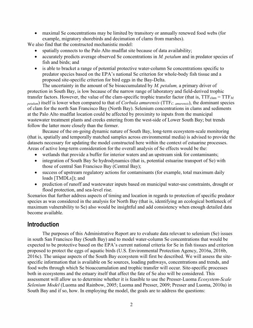
Abstract The U.S. Environmental Protection Agency (EPA) proposed Aquatic Life and Aquatic-

Dependent Wildlife Criteria for Selenium (Se) in California’s San Francisco Bay and Delta (Bay-Delta) in June 2016. Here we apply the same modeling methodology—Ecosystem-Scale Selenium Modeling—to an assessment of conditions and documentation of food webs of south San Francisco Bay (South Bay) as an exploratory framework in support of site-specific Se criteria development. Long-term datasets contribute to the basis for modeling, especially the 21-year collection of the clam Macoma petalum from a mudflat at the lower end of South Bay (Lower South Bay). As such, this is a working document that may serve as a basis to establish an understanding of the specifics of Se biodynamics within the estuary and reduce uncertainties about how to protect it. This approach brings together the main factors involved in toxicity: likelihood of high exposure, inherent species sensitivity, and the behavioral ecology (for example, demographics and life history) of an organism in terms of susceptibility to a reproductive toxicant. Species sensitivity is represented here by use of the EPA’s current national tissue Se criterion for fish or that proposed to protect the eggs of aquatic birds for the Bay-Delta (U.S. Environmental Protection Agency, 2016a, 2016b, 2016c). This report also strives to bring together findings and field data across a body of literature for South Bay to provide an integrative assessment.

We find an assemblage of site-specific conditions that could affect modeling: • associated urban processes such as discharges from municipal wastewater treatment plants and

drainage from mercury (Hg) mining and limestone extraction are sources of Se that characterize the Lower South Bay as the location of interest for Se exposure;

• hydrodynamics are lagoon-like (that is, less flushing), which sustains elevated nutrients and phytoplankton blooms;

• managed freshwater sources are a major hydrodynamic component; • birds, in addition to fish, are prominent predators in South Bay; • wetland restoration has recently intervened to play a significant role in ecosystem function that

may include uptake of both Hg and Se; • the dietary food web of surficial-sediment to M. petalum is important because of the dominance

of this clam species and its elevated Se bioaccumulation potential compared to other local food webs; and

2

• maximal Se concentrations may be limited by transitory or annually renewed food webs (for example, migratory shorebirds and decimation of clams from marshes).

We also find that the constructed mechanistic model: • spatially connects to the Palo Alto mudflat site because of data availability; • accurately predicts average observed Se concentrations in M. petalum and in predator species of

fish and birds; and • is able to bracket a range of potential protective water-column Se concentrations specific to

predator species based on the EPA’s national Se criterion for whole-body fish tissue and a proposed site-specific criterion for bird eggs in the Bay-Delta. The uncertainty in the amount of Se bioaccumulated by M. petalum, a primary driver of

protection in South Bay, is low because of the narrow range of laboratory and field-derived trophic transfer factors. However, the value of the clam-specific trophic transfer factor (that is, TTFclam = TTFM.

petalum) itself is lower when compared to that of Corbula amurensis (TTFC. amurensis), the dominant species of clam for the north San Francisco Bay (North Bay). Selenium concentrations in clams and sediments at the Palo Alto mudflat location could be affected by proximity to inputs from the municipal wastewater treatment plants and creeks entering from the west-side of Lower South Bay; but trends follow the latter more closely than the former.

Because of the on-going dynamic nature of South Bay, long-term ecosystem-scale monitoring (that is, spatially and temporally matched samples across environmental media) is advised to provide the datasets necessary for updating the model constructed here within the context of estuarine processes. Areas of active long-term consideration for the overall analysis of Se effects would be the:

• wetlands that provide a buffer for interior waters and an upstream sink for contaminants; • integration of South Bay Se hydrodynamics (that is, potential estuarine transport of Se) with

those of central San Francisco Bay (Central Bay); • success of upstream regulatory actions for contaminants (for example, total maximum daily

loads [TMDLs]); and • prediction of runoff and wastewater inputs based on municipal water-use constraints, drought or

flood protection, and sea-level rise. Scenarios that further address aspects of timing and location in regards to protection of specific predator species as was considered in the analysis for North Bay (that is, identifying an ecological bottleneck of maximum vulnerability to Se) also would be insightful and add consistency when enough detailed data become available.

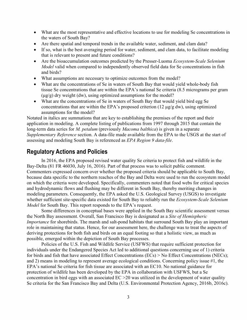
Introduction The purposes of this Administrative Report are to evaluate data relevant to selenium (Se) issues

in south San Francisco Bay (South Bay) and to model water-column Se concentrations that would be expected to be protective based on the EPA’s current national criteria for Se in fish tissues and criterion proposed to protect the eggs of aquatic birds (U.S. Environmental Protection Agency, 2016a, 2016b, 2016c). The unique aspects of the South Bay ecosystem will first be described. We will assess the site-specific information that is available on Se sources, loading pathways, concentrations and trends, and food webs through which Se bioaccumulation and trophic transfer will occur. Site-specific processes both in ecosystems and the estuary itself that affect the fate of Se also will be considered. This assessment will allow us to determine whether it is feasible to use the Presser-Luoma Ecosystem-Scale Selenium Model (Luoma and Rainbow, 2005; Luoma and Presser, 2009; Presser and Luoma, 2010a) in South Bay and if so, how. In employing the model, the goals are to address the questions:

3

• What are the most representative and effective locations to use for modeling Se concentrations in the waters of South Bay?

• Are there spatial and temporal trends in the available water, sediment, and clam data? • If so, what is the best averaging period for water, sediment, and clam data, to facilitate modeling

that is relevant to present and future conditions? • Are the bioaccumulation outcomes predicted by the Presser-Luoma Ecosystem-Scale Selenium

Model valid when compared to independently observed field data for Se concentrations in fish and birds?

• What assumptions are necessary to optimize outcomes from the model? • What are the concentrations of Se in waters of South Bay that would yield whole-body fish

tissue Se concentrations that are within the EPA’s national Se criteria (8.5 micrograms per gram (μg/g) dry weight (dw), using optimized assumptions for the model?

• What are the concentrations of Se in waters of South Bay that would yield bird egg Se concentrations that are within the EPA’s proposed criterion (12 μg/g dw), using optimized assumptions for the model?

Notated in italics are summations that are key to establishing the premises of the report and their application in modeling. A complete listing of publications from 1997 through 2015 that contain the long-term data series for M. petalum (previously Macoma balthica) is given in a separate Supplementary Reference section. A data-file made available from the EPA to the USGS at the start of assessing and modeling South Bay is referenced as EPA Region 9 data-file.

Regulatory Actions and Policies In 2016, the EPA proposed revised water quality Se criteria to protect fish and wildlife in the

Bay-Delta (81 FR 46030, July 16, 2016). Part of that process was to solicit public comment. Commenters expressed concern over whether the proposed criteria should be applicable to South Bay, because data specific to the northern reaches of the Bay and Delta were used to run the ecosystem model on which the criteria were developed. Specifically, commenters noted that food webs for critical species and hydrodynamic flows and flushing may be different in South Bay, thereby meriting changes in modeling parameters. Consequently, the EPA asked the U.S. Geological Survey (USGS) to investigate whether sufficient site-specific data existed for South Bay to reliably run the Ecosystem-Scale Selenium Model for South Bay. This report responds to the EPA’s request.

Some differences in conceptual bases were applied in the South Bay scientific assessment versus the North Bay assessment. Overall, San Francisco Bay is designated as a Site of Hemispheric Importance for shorebirds. The marsh and salt-pond habitats that surround South Bay play an important role in maintaining that status. Hence, for our assessment here, the challenge was to treat the aspects of deriving protections for both fish and birds on an equal footing so that a holistic view, as much as possible, emerged within the depiction of South Bay processes.

Policies of the U.S. Fish and Wildlife Service (USFWS) that require sufficient protection for individuals under the Endangered Species Act led to additional questions concerning use of 1) criteria for birds and fish that have associated Effect Concentrations (ECs) > No Effect Concentrations (NECs); and 2) means in modeling to represent average ecological conditions. Concerning policy issue #1, the EPA’s national Se criteria for fish tissue are associated with an EC10. No national guidance for protection of wildlife has been developed by the EPA in collaboration with USFWS, but a Se concentration in bird eggs with an associated EC >20 was utilized in the development of water quality Se criteria for the San Francisco Bay and Delta (U.S. Environmental Protection Agency, 2016b, 2016c).

4

In the future, several direct remedies for both issues could be instituted through modeling scenarios that address the levels of protectiveness and predict maximum stringency.

However, scientifically the scenarios developed here do indirectly address development of maximum stringency through the use of a range of food-web and partitioning factors. Additionally, derivation and validation of protection for South Bay was not simplistic, but rather based on consideration of categorized, ecologically-consistent datasets reflective of different site-specific conditions, time periods, and locations. This type of approach led to the use of a suite of concentrations and estimates of uncertainties that helped guide the choice of scenarios most likely to be protective given the limitations of the available datasets and currently known details of the estuarine and ecosystem processes of South Bay. For example, in the North Bay assessment, percentiles representing data for Carquinez Strait, rather than for the Bay as a whole, were the major focus of the analysis to quantify the influence of major refinery Se sources within modeling scenarios (Presser and Luoma, 2010b). Thus, Ecosystem-Scale Se Modeling quantifies, in a variety of data-driven ways, the underlying food-web and site-specific variables that are expressed throughout model development.

Overall it is important to understand the thesis on which Ecosystem-Scale Se Modeling was built when connecting modeling to regulations—the approach is not designed to provide a single choice for a site-specific criterion. The model is designed to:

• incorporate site-specific information into a guideline; • constrain variability in the choices of a guideline value (for example when calculating a

dissolved guideline from the fish tissue guideline); and • give regulators and stakeholders a sense for the outcome of different choices and why those

outcomes differ. There is some variability in the data available at every step in the model and choices must be made; ultimately modeling should give managers and regulators a well-defined strategy for understanding and constraining those choices within site-specific applications.

South San Francisco Bay Ecosystem San Francisco Bay generally consists of two embayments with contrasting characteristics

(Walters and others, 1985; fig. 1). The north arm is the drowned mouth of the Sacramento-San Joaquin Rivers that drains the interior valleys of California. It is dominated by strong tides and inflows from the two large river systems. North Bay is a classic partially mixed estuary with a consistent land-to-sea salinity gradient and waters that are often stratified with higher density seawater dominating deeper waters and lower density freshwater towards the surface.

5

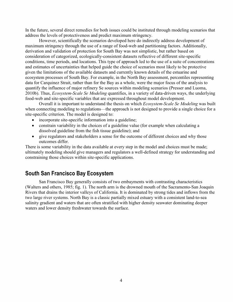
Figure 1. Map of San Francisco Bay system. Lower South Bay (LSB; blue box) is the area of primary interest with regard to selenium (Se). The map shows the urbanization of LSB and the extensive mosaic of sloughs, marshes, and salt ponds that are undergoing restoration. An intertidal mudflat near the highlighted city of Palo Alto (red X) is a focus of long-term monitoring of benthic food webs. The arrow in the North Bay points towards the remainder of the Northern Reach, which encompasses San Pablo Bay, Suisun Bay, Carquinez Strait, and further landward, the Sacramento-San Joaquin River Delta.

South Bay is a semi-enclosed embayment, which oceanographers describe as a “tidally oscillating lagoon with (seasonal) density-driven exchanges with the northern reach” (Walters and others, 1985). The data assessment that follows shows that Lower South Bay (LSB), south of the Dumbarton Bridge (outlined in fig. 1), is the area of South Bay that is of greatest concern with regard to

6

Se. At the south terminus, LSB is an especially shallow sub-embayment connected to a “network of sloughs, marshes and salt ponds undergoing restoration to wetlands” (Crauder and others, 2016). Several creeks and streams discharge to LSB after traversing a heavily urbanized landscape (see details in the Sources of Selenium section). Streamflow occurs predominantly during the rainy season of November–March when streams carry untreated urban runoff, as well as runoff from an upstream legacy mining district and an active limestone quarry into LSB. LSB also receives 120 million gallons per day of heavily treated waste-water effluent from Publically Owned Treatment Works (POTWs; Crauder and others, 2016). Especially during the dry season, the municipal waste effluents are the largest source of freshwater input to South Bay (East Bay Dischargers Authority, 2015). The large volume of POTW effluents entering LSB creates a persistent weak salinity gradient from lower values in the south to higher values toward the sea in the north.

Residence times of water masses, which influence the fate of Se, vary seasonally and differ between North Bay and South Bay. In the northern reach, residence times are on the order of days during periods of high river discharge in winter and spring, and weeks (sometimes more than a month) during summer-fall periods (Conomos, 1979). South Bay, and especially LSB, is relatively stagnant during much of the year compared to North Bay. Residence times are complex (Gross and others, 1999) but broad estimates suggest they are on the order of several months (Walters and others, 1985). Relatively rapid “flushing” of accumulated water-column constituents in South Bay usually occurs during a short period when river inflows from the north exceed a threshold that pushes them over a shallow shelf (San Bruno Shoals) that separates Central Bay from South Bay (Luoma and Cain, 1979; fig. 1). This occurs only when river inflows from the north are at their highest in spring and early summer. The penetration of freshwater from the north into South Bay during these periods causes rapid density-driven exchanges with Central Bay and the sea. LSB is affected by this seasonal flushing, but otherwise has limited net tidal exchange with the rest of the Bay. Much of the water that leaves LSB on ebb tides returns on flood tides (Crauder and others, 2016). The limited exchange leads to biogeochemical and ecological conditions in LSB that are somewhat distinct from the rest of San Francisco Bay including the highest nutrient concentrations and phytoplankton biomass anywhere in San Francisco Bay (Crauder and others, 2016).

Because it is a shallow embayment, persistent winds and the diurnal tides are effective in mixing South Bay waters vertically. This reduces the frequency of stratification and thus allows bottom-dwelling organisms to access phytoplankton from surface waters. Phytoplankton blooms occur in South Bay mainly during the short period in spring when South Bay stratifies, separating the phytoplankton from the benthos. A combination of calm winds, weak tides, and freshwater inflow from the north are necessary to induce stratification (Cloern, 1991). The rest of the year, wind and tide-driven mixing constantly move waters to the bottom. This physical trait influences South Bay ecology, resulting in a productive benthic community where organisms like filter-feeding bivalves are an important component. Except during periods of stratification this community is able to strip most phytoplankton from the water-column, facilitating nutrient (and Se) transfer into the benthos. In turn, during each fall, predation by migratory and resident birds (Thompson and others, 2008), fish, and invertebrates (Cloern and others, 2007; 2010) decimate bivalve communities (Crauder and others, 2016), but larvae reinitiate population growth each spring.

Nutrient loads to LSB have declined over the years, but are still 2.5–4-fold higher than to any other San Francisco Bay sub-embayment (Crauder and others, 2016). The small volume of LSB and the slower flushing rate allow these nutrients to accumulate to the highest concentrations observed anywhere in the Bay. Spatially, nutrient concentrations increase four-fold from the Dumbarton Bridge south toward the mouths of watershed sloughs (for example, Coyote Creek and Artesian Slough, the

7

discharge point for San Jose-Santa Clara Regional Wastewater Treatment Facility). This gradient is driven by proximity to sources, dilution with the rest of South Bay, and phytoplankton uptake (Crauder and others, 2016). The processes that influence nutrient concentrations would also be expected to influence Se concentrations, creating a similar tendency to accumulate elevated concentrations in the LSB relative to the rest of the Bay and an increasing gradient toward sources of input.

The benthic invertebrate assemblages differ between South Bay and North Bay. The assemblage in Suisun Bay (the area of primary interest in North Bay with regard to Se) is described by Thompson and others (2013) as a low-diversity oligohaline (low salinity) assemblage. The Suisun-Bay assemblage is simplified because few organisms can survive the extreme fluctuations in salinity within a year (Melwani and Thompson, 2007). The filter feeding, invasive species Corbula amurensis is the predominant bivalve in Suisun Bay. This species is primarily found in low salinity waters. In waters where higher salinities can occur, as in South Bay, C. amurensis populations are less persistent and less abundant, possibly because their metabolic rates increase to facilitate osmoregulation and they compensate by increasing their filter-feeding rate (Paganini and others, 2010).

South Bay is occupied by a mesohaline (moderately salty compared to seawater) invertebrate assemblage that is more diverse than that found in Suisun Bay (Thompson and Parchaso, 2012; Crauder and others, 2016). Salinity fluctuations in South Bay (appendix fig. A1) are rarely as extreme as in North Bay (Presser and Luoma, 2010b). Periods of low salinity are of short duration in all but the wettest years. The dominant, large filter-feeding bivalves include M. petalum, Musculista senhousia, Mytilus c.f. edulis, Mya arenaria, C. amurensis, and Venerupis japonica. M. petalum is a burrowing bivalve that can filter-feed, but has a slow filtration rate because its morphology is that of a deposit feeder. It predominantly feeds on benthic algae living on the surface sediments of the mudflats and shallow subtidal zones.

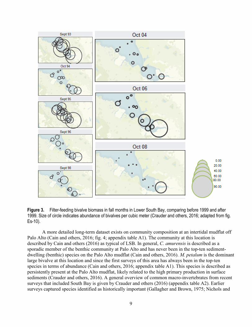
C. amurensis is of particular interest in San Francisco Bay because it bioaccumulates Se with great efficiency, passing this Se on to its predators. C. amurensis occurred with some regularity before 1999 in South Bay and especially in LSB (Melwani and Thompson, 2007; Crauder and others, 2016), although it was rarely as dominant as it is in North Bay. After 1999, a decline occurred in the relative abundance of filter-feeding benthos in South Bay (fig. 2) that included a decline in the abundance of at least some bivalves including C. amurensis (fig. 3). The cause was a natural shift in ocean conditions corresponding with an increase in benthic predators (for example Crangon shrimp; juvenile Dungeness crab, Cancer magister; and the English sole, Parophyrys vetulus; Cloern and others, 2007). The biomass of surface-sediment feeders did not decline, many of which, like M. petalum, live deeper within the sediments (Crauder and others, 2016). This change persists to the present in South Bay, at least north of the Dumbarton Bridge (the seaward boundary of LSB). In LSB, the abundance of large bivalves like C. amurensis after 1999 appeared to be influenced by salinities and residence times. C. amurensis was somewhat abundant in wet years, like 2006, but rare in the dry or average rainfall years (fig. 3) between 1999 and 2009 (Crauder and others, 2016). Published data on community composition were only available up to 2009. In the only recent studies, Thompson and others (oral commun., May 15, 2017) found C. amurensis was extremely abundant in South Bay in the very high flow year of 2017, reinforcing the evidence of high C. amurensis abundance when salinities are lower in years of high precipitation. In addition, Parchaso and others (2015) described the benthic community within the creeks and sloughs of LSB to begin to establish a record for some of the buffer zones that surround the bay.

8

A B

Figure 2. Percent of the benthic community comprised of large filter-feeding bivalves, including C. amurensis, and ascidians (sea squirts) from A, the western shoal (south of the Dumbarton Bridge) and B, the eastern shoal (north of the Dumbarton Bridge) (Crauder and others, 2016; adapted from fig. 4-6).

9

Figure 3. Filter-feeding bivalve biomass in fall months in Lower South Bay, comparing before 1999 and after 1999. Size of circle indicates abundance of bivalves per cubic meter (Crauder and others, 2016; adapted from fig. Es-10).

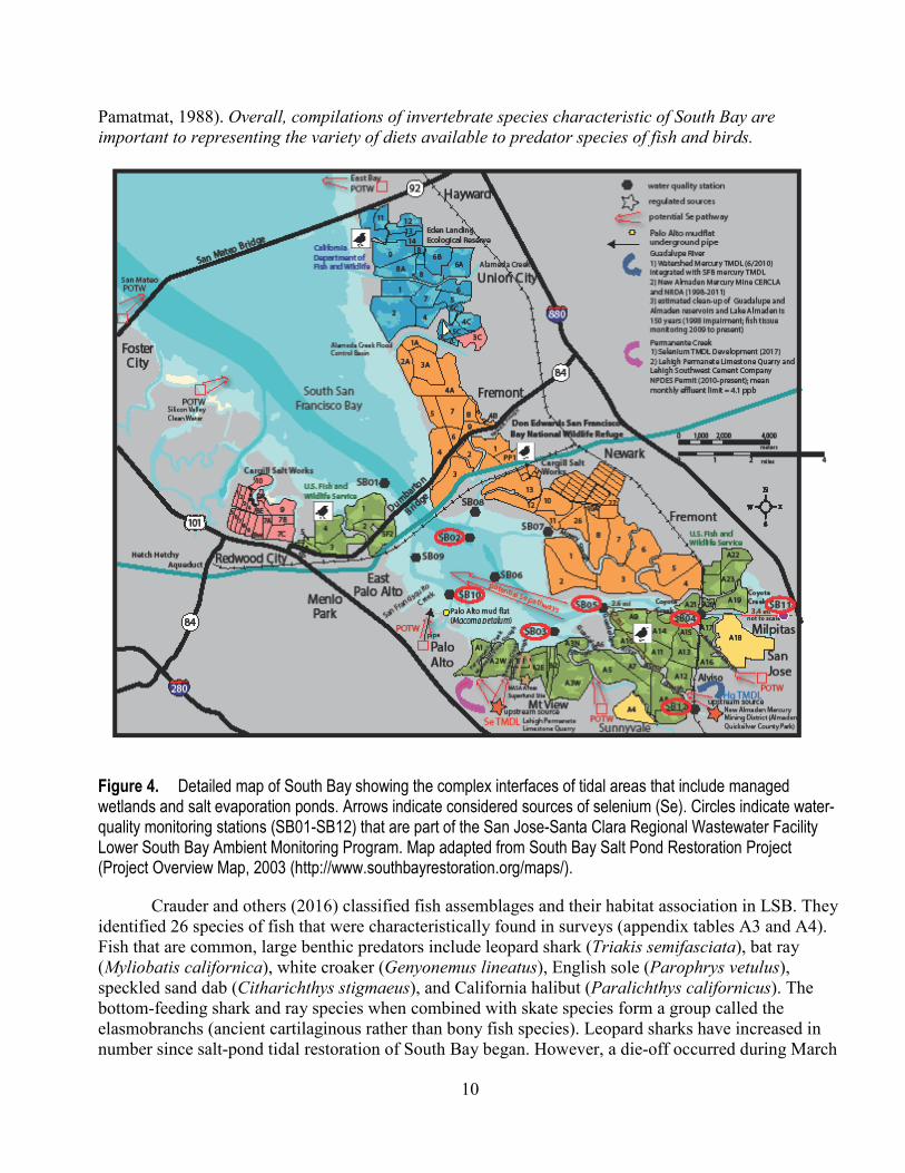
A more detailed long-term dataset exists on community composition at an intertidal mudflat off Palo Alto (Cain and others, 2016; fig. 4; appendix table A1). The community at this location is described by Cain and others (2016) as typical of LSB. In general, C. amurensis is described as a sporadic member of the benthic community at Palo Alto and has never been in the top-ten sediment-dwelling (benthic) species on the Palo Alto mudflat (Cain and others, 2016). M. petalum is the dominant large bivalve at this location and since the first surveys of this area has always been in the top-ten species in terms of abundance (Cain and others, 2016; appendix table A1). This species is described as persistently present at the Palo Alto mudflat, likely related to the high primary production in surface sediments (Crauder and others, 2016). A general overview of common macro-invertebrates from recent surveys that included South Bay is given by Crauder and others (2016) (appendix table A2). Earlier surveys captured species identified as historically important (Gallagher and Brown, 1975; Nichols and

10

Pamatmat, 1988). Overall, compilations of invertebrate species characteristic of South Bay are important to representing the variety of diets available to predator species of fish and birds.

Figure 4. Detailed map of South Bay showing the complex interfaces of tidal areas that include managed wetlands and salt evaporation ponds. Arrows indicate considered sources of selenium (Se). Circles indicate water-quality monitoring stations (SB01-SB12) that are part of the San Jose-Santa Clara Regional Wastewater Facility Lower South Bay Ambient Monitoring Program. Map adapted from South Bay Salt Pond Restoration Project (Project Overview Map, 2003 (http://www.southbayrestoration.org/maps/).

Crauder and others (2016) classified fish assemblages and their habitat association in LSB. They identified 26 species of fish that were characteristically found in surveys (appendix tables A3 and A4). Fish that are common, large benthic predators include leopard shark (Triakis semifasciata), bat ray (Myliobatis californica), white croaker (Genyonemus lineatus), English sole (Parophrys vetulus), speckled sand dab (Citharichthys stigmaeus), and California halibut (Paralichthys californicus). The bottom-feeding shark and ray species when combined with skate species form a group called the elasmobranchs (ancient cartilaginous rather than bony fish species). Leopard sharks have increased in number since salt-pond tidal restoration of South Bay began. However, a die-off occurred during March

11

and April 2017 with an estimate in the hundreds to as much as one thousand individuals being affected during a period of heavy rains that decreased salinity in the Bay to a level not seen in the last 30 years. Bat rays have also increased in number but are affected by smaller die-offs when they become trapped in flooded salt ponds. The California skate (Raja inornate), although also a benthic predator, is less common in South Bay. Smaller common predators include topsmelt (Atherinopos affinis), several species of gobies, and staghorn sculpin (Leptocottus armatus). In general, the exposure to Se of all of these species is likely different in South Bay than in North Bay at least partly because of the differences in the relative abundance of different benthic prey, especially in the last 15 years.

Crauder and others (2016) specifically noted that green sturgeon (Acipenser medirostris) and white sturgeon (Acipenser trensmontanus), which are native, anadromous, benthic predators are not commonly found in surveys in South Bay because they cannot migrate upstream from this system. However, both sturgeon species may use habitats in South Bay for brief periods of time. Green sturgeon was listed as a threatened species in 2006 (https://ecos.fws.gov/ecp0/profile/speciesProfile?s Id=2329). Crauder and others (2016) classified green sturgeon as rare in South Bay and white sturgeon as uncommon. Both species are of special interest in terms of conservation (Klimley and others, 2015) and with regard to Se bioaccumulation (U.S. Fish and Wildlife Service, 2008a; Presser and Luoma, 2013).

In terms of bird species, San Francisco Bay is recognized as a Site of Hemispheric Importance for shorebirds, the highest ranking possible (Pitkin and Wood, 2011; Donehower and others, 2013). San Francisco Bay provides habitat for the highest proportion of the total wintering and migrating shorebirds on the Pacific Coast compared to other wetlands. Seventy percent of birds that migrate on the flyway are estimated to spend some time each year in the estuary. The tidal and salt marshes of the estuary include the northernmost coastal breeding habitat for American avocet (Recurvirostra Americana) and black-necked stilt (Himantopus mexicanus). About 10 percent of the Pacific Coast’s endangered western snowy plovers (Charadrius nivosus nivosus) breed in the specific habitats afforded by South Bay. Avocets, stilts, and plovers are attracted to LSB’s area of highly saline salt-production ponds, where they can feed on Artemia franciscana, a local species of brine shrimp.

In a study of South Bay, the U.S. Fish and Wildlife Service (2008b) identified 43 species of locally-nesting marsh refuge birds that were common in the habitats of the Don Edwards National Wildlife Refuge (DENWR) in at least one season (fig. 4; appendix table A5). Also listed in appendix table A5 are 15 species of abundant or common shorebirds that are known to migrate through the refuge.

Species of aquatic birds that are endangered or threatened under the Endangered Species Act in LSB include Ridgway’s rail (Rallus obsoletus) (formerly California clapper rail; https://ecos.fws.gov/ecp0/profile/species Profile?spcode=B04A), western snowy plover (https://www.fws.gov/arcata/es/birds/ wsp/plover.html) and California least tern (Sternula antillarum browni) (https://www.fws.gov/sacramento/es_species/Accounts/Birds/es_ca-least-tern.htm) (appendix table A6). Ridgway’s rail is the subject of recent study because of a general loss of habitat due to sea-level rise (Overton and others, 2015). These three species were noted as present occasionally at the DENWR in 2008, but in 2015 Ridgway’s rail was found returning to restored ponds where they had previously flourished prior to salt harvesting. The eggs of the breeding western snowy plover are currently under attack by an expanding population of the California gull (Larus californicus), whose individuals also are attracted to the recently restored habitats. The California least tern does not nest locally, but abundant Forster’s terns (Sterna forsteri) that do nest locally could serve as possible surrogates in monitoring plans (Ackerman and others, 2014).

Additional information on feeding behavior and foraging guilds as a means of classification of bird species’ use of environmental resources is listed in appendix tables A5, A7, and A8. Listed as a

12

separate category of nesting or migratory bird species are those consuming molluscs because of their potential connection to local M. petalum food webs (De Graaf and others, 1985; tables A5 and A8). Some species can display 1) overlapping designations (that is, molluscivore or crustaceavore or insectivore); 2) a change of feeding habit during breeding period; or 3) a generalized omnivore designation (De Graaf,and others, 1985). Sorting and narrowing of the local species by these types of characteristics (for example, diet, habitat-use, or regulatory status; tables A5–A8) are important in developing modeling scenarios to establish a range of potential environmental risk. For example, the locally nesting molluscivorous Ridgway’s rail provides an example of a species consuming a Se bioaccumulator that is directly linked to reproduction in South-Bay habitats (tables A5 and A8), while migratory molluscivorous species (table A5) provide examples relevant to transitory use of LSB habitats.

Influence of Ecosystem Characteristics on Selenium The unique physical, biogeochemical, and ecological conditions in South Bay, and especially

LSB, could have implications for Se for the fate and effects. Selenium concentrations in waters and sediments of LSB will be influenced by a number of processes, including:

• increased inputs by runoff in early winter through spring; • density-driven exchange with Central Bay in mid-spring; • reduced flushing from summer until rainfall begins again in fall; and • winnowing (removal) of fine-grained sediments from the bed by daily winds and tides in

summer. High phytoplankton biomass and long residence times could affect

• biotransformation of incoming Se; • stripping of Se from the water-column; • release of Se from primary producers and microorganisms; and • changes in speciation of Se in the water-column.

The long residence time, high nutrient inputs, and deposition of fine-grained sediments allow some degree of oxygen-depletion in the sediments, especially in the sub-surface (Crauder and others, 2016). This could also affect Se transformation (Luoma and Presser, 2009) and speciation on suspended particulate material and in sediments (Meseck and Cutter, 2012). Because these processes vary in intensity and length from year to year, seasonal cycles in Se concentrations and bioavailability are expected to be complex.

Extensive wetland restoration in LSB has the potential to affect Se inputs, storage, and outputs (that is, Se mass balance). For 150 years, artificial salt ponds surrounded LSB. The salt ponds were diked off from local streams and the interior bay waters to facilitate production of commercial salt. Production of salt ended in 1993 (Takekawa and others, 2001). Since then, dikes have been broken and wetlands are being restored over much of the shoreline of LSB. The overall project will restore 15,000 acres of industrial salt ponds to a mosaic of tidal wetlands and other managed habitats over a fifty-year period (http://www.southbayrestoration.org/documents/technical/; U.S. Fish and Wildlife Service and California Department of Fish and Game, 2007; Beller and others, 2013; Ackerman and others, 2014). Exchange of water within these wetlands with waters from the LSB, sloughs, and streams could allow Se to be trapped in the wetlands, removing it from LSB. Thus, restoration could have long-term influences on the Se exposure of both the food webs of LSB and the wetlands themselves.

In a corollary concern, research on mercury (Hg) in food webs in San Francisco Bay has intensified as large-scale tidal-wetland restoration actions have been planned and implemented (Davis

http://www.southbayrestoration.org/documents/technical/

13

and others, 2003; Schwarzbach and Adelsbach, 2003). Specifically for South Bay where restoration of wetlands and salt ponds was initiated in 2003–2004, several lines of evidence from field studies in South Bay indicate that Hg contamination may be impairing reproduction in breeding birds (Ackerman and others, 2014). For example, Hg benchmarks for high risk of reproductive impairment in Forster’s terns have been exceeded in both blood samples (48 percent) and egg samples (98 percent). Since 2010, Hg has been regulated within an integrated total maximum daily load (TMDL) approach for the Guadalupe River watershed and South Bay (see fig. 4 and additional details in the Sources of Selenium section) (California Regional Water Quality Control Board, 2008). Complex Hg and Se interactions are documented in birds and fish both in the laboratory and in some (but not all) locations in the field (Heinz and Hoffman, 1998; Penglase and others, 2014). Antagonistic (that is, mitigating) effects on bioaccumulation, linked bioaccumulation, and synergistic effects on reproduction are examples of ways that Hg and Se can interact where exposures are constant or controlled. Both Hg and Se exposures are annually variable, have multifaceted spatial patterns, and have changed over time in LSB, adding to the complexity of any Hg-Se interactions. In these circumstances, such interactions are typically difficult to document and poorly understood. This is the case in wetlands and salt ponds of South Bay.

Ecological factors also can cause variability in the exposure of predators to Se in South Bay. Composition of food webs and the inherent tendency of different organisms in the food web to accumulate Se are important (Luoma and Presser, 2009). Selenium bioaccumulation in individuals also can vary if environmental conditions affect feeding rates or food composition affects assimilation efficiencies (Luoma and Rainbow, 2005). In North Bay, benthic predators, especially those that eat bivalves, accumulated the highest Se concentrations when compared to those predators eating from the water-column (Stewart and others, 2004). The dominance of C. amurensis in the benthos in Suisun Bay contributed to the elevated Se concentrations found in predators that feed on clams (for example, white and green sturgeon). In LSB, M. petalum is the species of primary interest because of its persistent abundance, its occurrence throughout LSB, its size (which makes it and its siphons a desirable food item), and the availability of a long-term dataset on Se concentrations in its tissue. Both laboratory studies and field data show that bivalves like M. petalum, which are dominant in LSB, bioaccumulate Se less efficiently than the North Bay dominant C. amurensis; but more efficiently than zooplankton and benthic invertebrates that are not bivalves. In this report, predictions of protective water-column concentrations in South Bay will use M. petalum as an indicator for the dominant bivalves. But scenarios that include C. amurensis in the diet of predators will also be presented to account for the wettest of years when C. amurensis can be abundant

White sturgeon, white croaker, and leopard shark are 1) fish species for which Se data exist; and 2) benthic predators that include bivalves as a component in their diet. Thus, they will be emphasized in this report. Comparisons between predicted Se uptake in these species and field observations can be used to test the validity of the model for predicting water-column Se concentrations that would be protective for fish.

Birds that are benthic predators are also of primary interest in South Bay; especially benthic predators listed as species of regulatory concern (appendix tables A6 and A8). Selenium concentrations in the eggs of Forster’s tern were determined in 2009 and 2014 as part of regional monitoring programs and can be used to validate how well the model predicts water-column Se concentrations that would be protective for birds. Forster’s tern is a reasonable surrogate for the endangered California least tern.

Enough data are available on Se sources and concentrations in the environment and food webs of South Bay (especially LSB) to develop an Ecosystem-Scale Selenium Model. However, it is important to document choices of data that were used in that model and to provide an ecosystem context to interpret model outcomes.

14

Sources of Selenium in South Bay South Bay is a densely populated urban landscape. The watersheds of all of the streams that

discharge to LSB are heavily utilized and each individual stream acts as a channel for a specific waste-water treatment facility or industry (fig. 4). Discharges to the LSB can be affected by their pathways to the open South Bay waters (fig. 4). For example, the type of extensive wetland and salt pond habitats of LSB that provides transitional zones are known to passively treat Se (Presser and Piper, 1998; Skorupa, 1998; Amweg and others, 2003). The overall consequence of these processes may lead to a reduction of Se concentrations in the water-column, but an uptake of Se into local ecosystem components.

Three waste treatment facilities that discharge Se to LSB on a nearly continuous basis are: • Palo Alto POTW (PA-POTW); • San Jose-Santa Clara Regional Wastewater Facility (SJ-SC RWF); and • Sunnyvale POTW (SV-POTW) (fig. 4).

Additional facilities discharge treated wastes north of the Dumbarton and San Mateo bridges as illustrated in figure 4.

Streams, sloughs, and a channel that contribute Se to LSB on a seasonal basis include: • Coyote Creek which is regulated by Anderson Dam; • Guadalupe River which discharges through Alviso Slough; • Artesian Slough which receives the effluent of the SJ-SC RWF; • Guadalupe Slough which receives the effluent of the SV-POTW; and • a small channel in an intertidal mudflat which receives the effluent of the PA-POTW through an

underground pipe. (Bay Area Stormwater Management Agencies Association, 2013; San Jose-Santa Clara Regional Wastewater Facility, 2016; Cain and others, 2016; fig. 4).

In terms of specific contributing sources, Lehigh Permanente Limestone Quarry (LPL Quarry) is an upstream source of Se mainly thought to be caused by emergent ground water (California Regional Water Quality Control Board, 2015). The LPL Quarry is under a court order to reduce and treat Se because of National Pollutant Discharge Elimination System (NPDES) permit violations and a TMDL assessment for Se is under development (California Regional Water Quality Control Board, 2014, 2015; http://www.waterboards.ca.gov/sanfranciscobay/water_issues/hot_topics/lehigh.shtml). Water-column Se concentrations of as much as 75 micrograms per liter (µg/L) serve as the influent to a recently developed treatment plant that has a monthly mean effluent limit of 4 µg/L. The treated discharge enters both Permanente and Stevens creeks (fig. 4) at certain times of the year. Concentrations measured at stations nearest the LSB range from 0.4 to 3.4 µg/L.

The headwaters of the Guadalupe River drain an upstream area where Hg mining took place historically (New Almaden Quicksilver County Park encompasses New Almaden Mercury Mining District [New Almaden]; Thomas and others, 2002; California Regional Water Quality Control Board, 2008). The remnants of mining have caused elevated Hg in fish in the lake and three reservoirs within the watershed. Health advisories are in place and Hg removal, restoration, and recovery actions are estimated to take up to 120 years (http://www.valley water.org/mercury.aspx). In general, Se-bearing minerals can be associated with Hg deposits. For example, Se is documented as a contaminant of concern in the drainage from New Idria Mercury Mining District in the Coast Ranges of the western San Joaquin Valley of California (U.S. Environmental Protection Agency, 2010; https://yosemite.epa.gov/ r9/sfund/r9sfdocw.nsf/ViewBy EPAID/CA0001900463). So, there is reason to expect that this source of Hg could also be a source of Se (Ackerman and others, 2014). Recent limited analyses for Hg and Se at a downstream site in the Guadalupe River watershed are available as part of an urban pollutant loading

15

study (2003–2014; McKee and others, 2017). However, a comprehensive study of Se mobilization in the area of New Almaden has not been conducted.

In terms of connection of the Guadalupe River watershed to the LSB, clean-up of New Almaden as a designated superfund site has been taking place since 1998. Additionally there is a Hg TMDL in place for the river that is integrated with the estuary since 2010 (California Regional Water Quality Control Board, 2008). Hence, long-term remediation activities both at New Almaden and the LPL Quarry have the potential to affect Se concentrations in LSB.

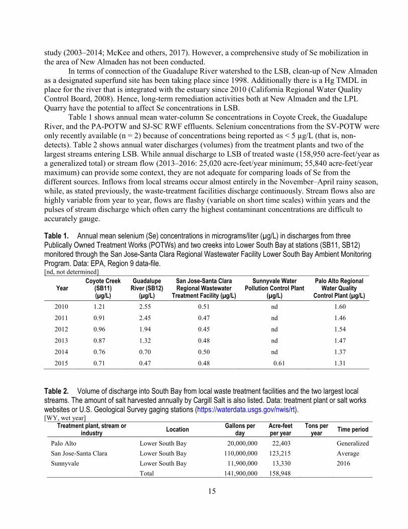
Table 1 shows annual mean water-column Se concentrations in Coyote Creek, the Guadalupe River, and the PA-POTW and SJ-SC RWF effluents. Selenium concentrations from the SV-POTW were only recently available (n = 2) because of concentrations being reported as < 5 µg/L (that is, non-detects). Table 2 shows annual water discharges (volumes) from the treatment plants and two of the largest streams entering LSB. While annual discharge to LSB of treated waste (158,950 acre-feet/year as a generalized total) or stream flow (2013–2016: 25,020 acre-feet/year minimum; 55,840 acre-feet/year maximum) can provide some context, they are not adequate for comparing loads of Se from the different sources. Inflows from local streams occur almost entirely in the November–April rainy season, while, as stated previously, the waste-treatment facilities discharge continuously. Stream flows also are highly variable from year to year, flows are flashy (variable on short time scales) within years and the pulses of stream discharge which often carry the highest contaminant concentrations are difficult to accurately gauge.

Table 1. Annual mean selenium (Se) concentrations in micrograms/liter (µg/L) in discharges from three Publically Owned Treatment Works (POTWs) and two creeks into Lower South Bay at stations (SB11, SB12) monitored through the San Jose-Santa Clara Regional Wastewater Facility Lower South Bay Ambient Monitoring Program. Data: EPA, Region 9 data-file. [nd, not determined]

Year Coyote Creek

(SB11) (µg/L)

Guadalupe River (SB12)

(µg/L)

San Jose-Santa Clara Regional Wastewater

Treatment Facility (µg/L)

Sunnyvale Water Pollution Control Plant

(µg/L)

Palo Alto Regional Water Quality

Control Plant (µg/L) 2010 1.21 2.55 0.51 nd 1.60

2011 0.91 2.45 0.47 nd 1.46

2012 0.96 1.94 0.45 nd 1.54

2013 0.87 1.32 0.48 nd 1.47

2014 0.76 0.70 0.50 nd 1.37

2015 0.71 0.47 0.48 0.61 1.31

Table 2. Volume of discharge into South Bay from local waste treatment facilities and the two largest local streams. The amount of salt harvested annually by Cargill Salt is also listed. Data: treatment plant or salt works websites or U.S. Geological Survey gaging stations (https://waterdata.usgs.gov/nwis/rt). [WY, wet year]

Treatment plant, stream or industry Location Gallons per

day Acre-feet per year

Tons per year Time period

Palo Alto Lower South Bay 20,000,000 22,403 Generalized San Jose-Santa Clara Lower South Bay 110,000,000 123,215 Average Sunnyvale Lower South Bay 11,900,000 13,330 2016 Total 141,900,000 158,948

16

Treatment plant, stream or industry Location Gallons per

day Acre-feet per year

Tons per year Time period

Silicon Valley Clean Water1 North of Dumbarton Bridge 29,000,000 32,484 2 Generalized San Mateo North of San Mateo Bridge 12,000,000 13,442 Generalized East Bay Dischargers

Authority North of San Mateo Bridge 119,000,000 133,297 Capacity

Total 160,000,000 179,223 Cargill Salt evaporation ponds 8,000 acres 500,000 Generalized

Guadalupe River USGS station #11169025 30,175 WY2016 (above highway 101) 21,969 WY2015 16,632 WY2014 37,150 WY2013 Coyote Creek USGS station #11172175 16,364 WY2016 (above highway 237) 12,639 WY2015 8,388 WY2014 18,667 WY2013

1 Formerly the South Bayside System Authority. 2 This plant has the capacity to nearly triple the daily capacity during the wet season (~97,452 acre-feet/year).

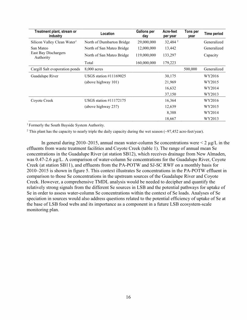
In general during 2010–2015, annual mean water-column Se concentrations were < 2 µg/L in the effluents from waste treatment facilities and Coyote Creek (table 1). The range of annual mean Se concentrations in the Guadalupe River (at station SB12), which receives drainage from New Almaden, was 0.47-2.6 µg/L. A comparison of water-column Se concentrations for the Guadalupe River, Coyote Creek (at station SB11), and effluents from the PA-POTW and SJ-SC RWF on a monthly basis for 2010–2015 is shown in figure 5. This context illustrates Se concentrations in the PA-POTW effluent in comparison to those Se concentrations in the upstream sources of the Guadalupe River and Coyote Creek. However, a comprehensive TMDL analysis would be needed to decipher and quantify the relatively strong signals from the different Se sources in LSB and the potential pathways for uptake of Se in order to assess water-column Se concentrations within the context of Se loads. Analyses of Se speciation in sources would also address questions related to the potential efficiency of uptake of Se at the base of LSB food webs and its importance as a component in a future LSB ecosystem-scale monitoring plan.

17

Figure 5. Comparison of water-column selenium (Se) concentrations in micrograms/liter (µg/L) for the Palo Alto Publicly Owned Treatment Works (PA-POTW) effluent, the San Jose-Santa Clara Regional Wastewater Facility (SJ-SC RWF) effluent, Coyote Creek (SB11), and the Guadalupe River (SB12) during the period January 2010–December 2015. Data: EPA, Region 9 data-file.

Selenium Concentrations in South Bay Waters Stations SB01 to SB12 in LSB (fig. 4) have been monitored for water-column Se concentrations

by the San Jose-Santa Clara Regional Wastewater Facility Lower South Bay Ambient Monitoring Program (SJ-SC MP) since 1997 with a hiatus between 1999 and mid-2002 (San Jose-Santa Clara Regional Wastewater Facility, 2016). These station locations (fig. 4) provide a monitoring grid essentially from landward to seaward and, hence, collected data can provide a strong line of evidence about the characteristics of Se inputs that contribute to the enrichment to the South Bay. Spatial details for each station are: SB11 and SB12 are upstream in Coyote Creek and inshore at the mouth of the

18

Guadalupe River, respectively; SB04 is near where Coyote Creek begins to enter the Bay; and SB05 is at the mouth of Alviso slough and receives inputs from both Coyote Creek and the Guadalupe River. SB03 is the most landward site towards the interior of LSB, and is directly influenced by inputs from Guadalupe Slough, Stevens Creek and Permanente Creek. SB10 is interior to LSB and just offshore from the USGS intertidal mudflat station at Palo Alto where surficial sediment and the clam M. petalum were collected. SB02 is located nearest the Dumbarton Bridge, where LSB meets Central South Bay. Early in the program, sampling occurred near monthly; but in later years, some sites were dropped. In 2010, sampling frequency at active sites was reduced to four times per year.

A series of graphs show water-column Se concentrations based on subsets of these water-quality sites: historical datasets for sites (SB06, 07, 08, 01, 02, 09) monitored from 1997–2009 (appendix figs. A2 and A3); and datasets for sites (SB11, 12, 04, 05, 03, 10, 02) monitored from 1997 to present to emphasize spatial connections of source streams and open-bay waters (figs. 6 and 7). In general, both the spatial gradients and temporal variability documented in this series of figures show that the region of South Bay of greatest interest with regard to Se is LSB. The spatial and temporal trends in LSB waters best reflect trends in stream/river inflows. But it is not possible to differentiate, from the existing data, the relative contribution to Se enrichment in LSB from sources in the stream/river inflows versus effluents from waste treatment facilities.

19

Figure 6. Fluctuations in water-column selenium (Se) concentrations micrograms/liter (µg/L) during 1997–2016: A, at the mouth of the Guadalupe River (SB12); B, landward in Coyote Creek (SB11); C, at lower Coyote Creek (SB04); and D, at the location in Lower South Bay that receives runoff from both Coyote Creek and the Guadalupe River (SB05). Samples were collected near monthly between 1997 and 2000, after which samples were collected four times per year. Declining Se concentrations with time are most evident at SB12 and SB05 primarily manifested as a decline in the magnitude of seasonal spikes in Se concentrations. Data: EPA, Region 9 data-file.

20

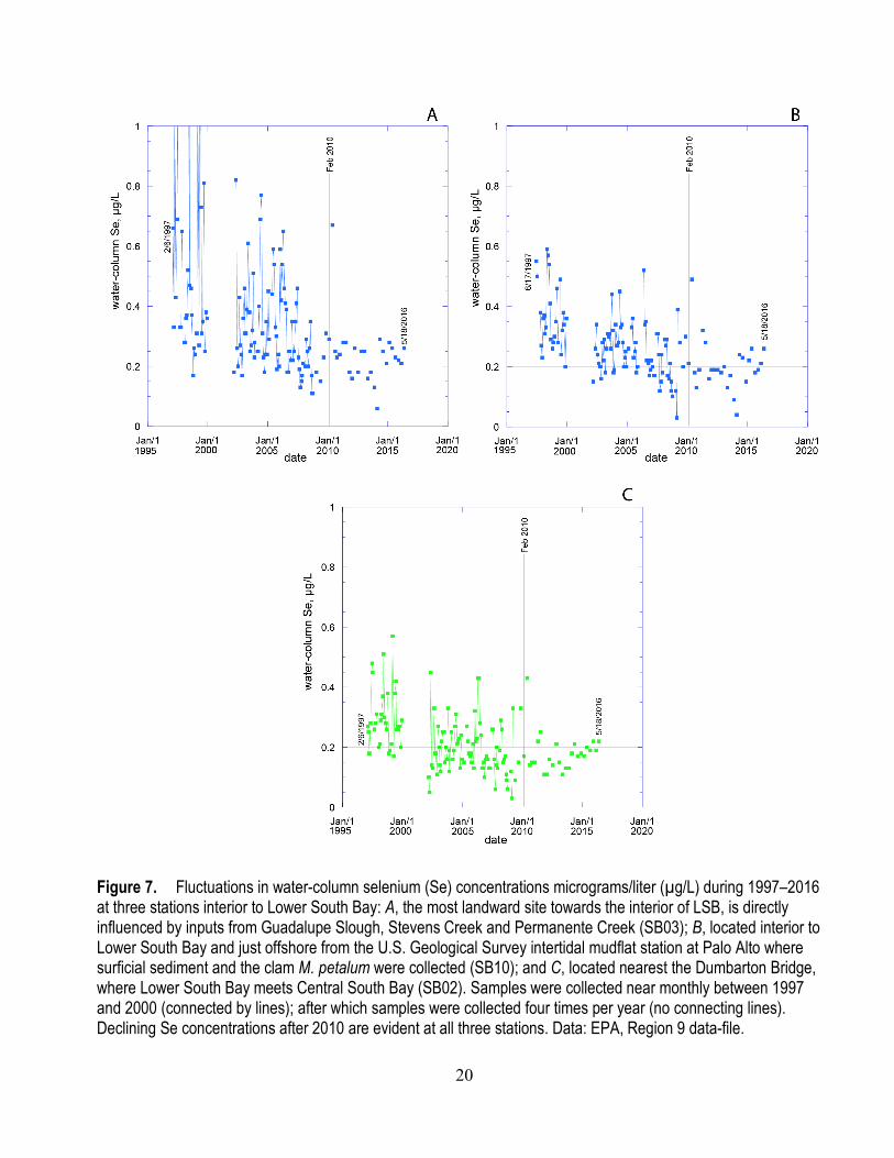
Figure 7. Fluctuations in water-column selenium (Se) concentrations micrograms/liter (µg/L) during 1997–2016 at three stations interior to Lower South Bay: A, the most landward site towards the interior of LSB, is directly influenced by inputs from Guadalupe Slough, Stevens Creek and Permanente Creek (SB03); B, located interior to Lower South Bay and just offshore from the U.S. Geological Survey intertidal mudflat station at Palo Alto where surficial sediment and the clam M. petalum were collected (SB10); and C, located nearest the Dumbarton Bridge, where Lower South Bay meets Central South Bay (SB02). Samples were collected near monthly between 1997 and 2000 (connected by lines); after which samples were collected four times per year (no connecting lines). Declining Se concentrations after 2010 are evident at all three stations. Data: EPA, Region 9 data-file.

21

In terms of individual station trends, monitoring across the record of data from 1997 to present for more landward sites (SB11, SB12, SB04, and SB05; fig. 6) shows that large spikes in Se concentrations occurred in the 1990s, but the magnitude of the seasonal spikes have generally lessened over time (through approximately 2007). Selenium concentrations in the Guadalupe River input to LSB (SB12) are especially characterized by short-term pulses of high Se concentrations early in each year. The maximum Se concentration at SB12 was nearly 8 µg/L in the late 1990s, but peak concentrations as high as 5–6 µg/L were observed each year up to 2008. Spikes were also evident at the station at the mouth of the Guadalupe River/Alviso Slough (SB05; fig. 6) and at a seaward site affected by Coyote Creek (SB04; fig. 6) where more muted peaks occurred. For seaward sites interior to LSB (SB02, SB03, and SB10; fig. 7), peaks also occurred in the earlier years of monitoring. In 2014–2016, peak water-column Se concentrations were <1.6 µg/L at the more landward stations (fig. 6). After 2011, no instances of concentrations >0.25 µg/L were observed at the most seaward station (SB02; fig. 7).

As noted previously (fig. 5), effluents from waste treatment facilities were characterized by smaller temporal fluctuations (for example PA-POTW) and declines in some inputs from the PA-POTW, but not from the SJ-SC RWF. Thus, the changing nature of Se concentrations during 1997–2010 in the interior of LSB more closely followed changes in the time series from the creek/sloughs than changes in effluents of the waste treatment facilities.

Explanations for the greatly reduced concentrations seen in 2010–2015 compared to the earlier monitoring period include:

• New Almaden mine-land restoration; • LPL Quarry regulatory guidance; • recent establishment of restored wetlands on the shoreline with which at least some of the

incoming streams, as well as some of the waste treatment effluents, now exchange; or • drought conditions that persisted from 2010–2015 (although water year 2011 was a wet year).

Drought and mine-land restoration would reduce runoff inputs. The strong ability of wetlands to sequester Se is well known, so the increasing area and maturity of the wetlands also could reduce water-column concentrations in LSB. It will be important to support LSB monitoring into the future to determine if these trends in improving Se conditions in LSB continue. Studies of Se in wetland food webs would also be advantageous given the active restoration that is occurring. For the purposes of modeling, it is clear that averaging over the entire time series would not be indicative of recent (and future) inputs. Therefore the focus of data used in this report and in the modeling will be the most recent 2010–2015 time period. The within-year variability is insufficiently consistent to average by season.

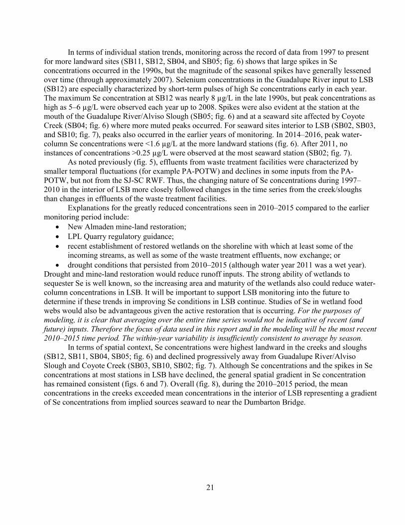
In terms of spatial context, Se concentrations were highest landward in the creeks and sloughs (SB12, SB11, SB04, SB05; fig. 6) and declined progressively away from Guadalupe River/Alviso Slough and Coyote Creek (SB03, SB10, SB02; fig. 7). Although Se concentrations and the spikes in Se concentrations at most stations in LSB have declined, the general spatial gradient in Se concentration has remained consistent (figs. 6 and 7). Overall (fig. 8), during the 2010–2015 period, the mean concentrations in the creeks exceeded mean concentrations in the interior of LSB representing a gradient of Se concentrations from implied sources seaward to near the Dumbarton Bridge.

22

Figure 8. Mean water-column selenium (Se) concentrations in micrograms per liter (μg/L) during 2010–2015 at two stations at outlets of creeks (SB11 and SB12) compared to four stations interior to Lower South Bay (SB02, SB03, SB04, SB10) and toward the Dumbarton Bridge at the mouth of Lower South Bay (SB02). Data: EPA, Region 9 data-file.

A conceptual spatial gradient of the pathways of Se into LSB is shown in figure 9. The plot was compiled from recent Se source and interior bay water-column Se concentrations to give context to the conclusions for LSB described above. Figure 9 is presented here as an experimental plot of the kind of conceptualization possible, but minimal data were available for building the plot. In detail, development of the gradient used mean Se concentrations from a set of water-quality monitoring stations (SB11, 12, 10, 05, 04, 03) with the most recent data (November 2009–May 2016) and recent monitoring of the effluents from the PA-POTW, SV-POTW and the SJ-SC RWF during 2015 and the LPL Quarry during 2013-2014 (fig. 4). As mentioned previously (Sources of Selenium section), both the LPL Quarry and New Almaden are under regulatory controls (fig. 4). The station depicted in red (SB01) is considered an anchor point, but the mean is from March 2002–May 2009. Additional stations (SB 06, 07, 08, 09) depicted in figure 4 were not used in development of the gradient because monitoring was discontinued in June 2009.

23

Figure 9. Conceptual spatial gradient of the pathways of selenium (Se) into Lower South Bay based solely on water-column Se concentrations in micrograms per liter (μg/L). The gradient is presented here as an experimental plot of the kind of conceptualization possible, but minimal data were available for building the plot. See additional details of 1) plot derivation in the Selenium Concentrations in South Bay Waters section; and 2) sampling stations in fig. 4. The spatial gradient is not underlain by data for flow or hydro-dynamic dimensions. The SB01 symbol is differentiated by color because of timing. Base map data 2017 © Google (imagery date September 2, 2017). The contour map was created in OriginPro 9.1 and merged with the base map by aligning matching coordinate locations between the base map and contour map.

Limitations to the derivation of the gradient (fig. 9) also include: • potential east-side Se sources are not depicted because of lack of data; • few data were available to derive a mean for the SV-POTW and LPL Quarry inputs; • only a water-column Se concentration (mean=2.4 µg/L) for a site in Stevens Creek (STE010)

that discharges proximate to the bay interface was used to represent the LPL Quarry source influence even though the adjacent Permanente Creek also receives permitted drainage (fig. 4); and

• the color-scale was adjusted for maximum color differentiation by using a water-column Se concentration of ≥1.6 µg/L, the mean water-column Se concentration of the PA POTW input. Additionally, the spatial plot (fig. 9) is not underlain by the dimensions of flow and

hydrodynamics. For example, POTWs and the creeks (table 2) discharge at high rates compared to the more sporadic discharges from New Almaden or the LPL Quarry. Hydrodynamic modeling could be added to the water-column spatial gradient in the future to generate an integrated multi-dimensional overview of LSB. Keeping all of these caveats in mind, the gradient nonetheless does frame the Palo

24

Alto mudflat location in relation to the relatively elevated exposures from the municipal wastewater treatment plants and creeks entering from the west-side of LSB (fig. 9).

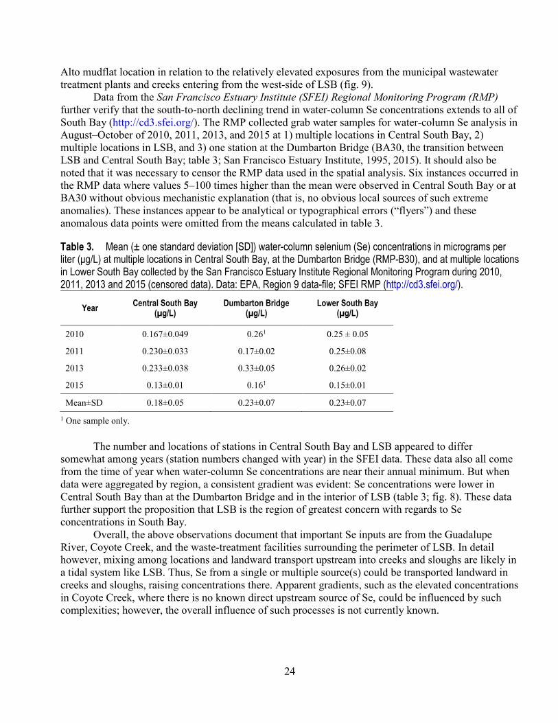
Data from the San Francisco Estuary Institute (SFEI) Regional Monitoring Program (RMP) further verify that the south-to-north declining trend in water-column Se concentrations extends to all of South Bay (http://cd3.sfei.org/). The RMP collected grab water samples for water-column Se analysis in August–October of 2010, 2011, 2013, and 2015 at 1) multiple locations in Central South Bay, 2) multiple locations in LSB, and 3) one station at the Dumbarton Bridge (BA30, the transition between LSB and Central South Bay; table 3; San Francisco Estuary Institute, 1995, 2015). It should also be noted that it was necessary to censor the RMP data used in the spatial analysis. Six instances occurred in the RMP data where values 5–100 times higher than the mean were observed in Central South Bay or at BA30 without obvious mechanistic explanation (that is, no obvious local sources of such extreme anomalies). These instances appear to be analytical or typographical errors (“flyers”) and these anomalous data points were omitted from the means calculated in table 3.

Table 3. Mean (± one standard deviation [SD]) water-column selenium (Se) concentrations in micrograms per liter (μg/L) at multiple locations in Central South Bay, at the Dumbarton Bridge (RMP-B30), and at multiple locations in Lower South Bay collected by the San Francisco Estuary Institute Regional Monitoring Program during 2010, 2011, 2013 and 2015 (censored data). Data: EPA, Region 9 data-file; SFEI RMP (http://cd3.sfei.org/).

Year Central South Bay (µg/L)

Dumbarton Bridge (µg/L)

Lower South Bay (µg/L)

2010 0.167±0.049 0.261 0.25 ± 0.05

2011 0.230±0.033 0.17±0.02 0.25±0.08

2013 0.233±0.038 0.33±0.05 0.26±0.02

2015 0.13±0.01 0.161 0.15±0.01

Mean±SD 0.18±0.05 0.23±0.07 0.23±0.07 1 One sample only.

The number and locations of stations in Central South Bay and LSB appeared to differ somewhat among years (station numbers changed with year) in the SFEI data. These data also all come from the time of year when water-column Se concentrations are near their annual minimum. But when data were aggregated by region, a consistent gradient was evident: Se concentrations were lower in Central South Bay than at the Dumbarton Bridge and in the interior of LSB (table 3; fig. 8). These data further support the proposition that LSB is the region of greatest concern with regards to Se concentrations in South Bay.

Overall, the above observations document that important Se inputs are from the Guadalupe River, Coyote Creek, and the waste-treatment facilities surrounding the perimeter of LSB. In detail however, mixing among locations and landward transport upstream into creeks and sloughs are likely in a tidal system like LSB. Thus, Se from a single or multiple source(s) could be transported landward in creeks and sloughs, raising concentrations there. Apparent gradients, such as the elevated concentrations in Coyote Creek, where there is no known direct upstream source of Se, could be influenced by such complexities; however, the overall influence of such processes is not currently known.

25

Selenium Concentrations in South Bay Sediments Long-term time series and spatial data also exist for Se concentrations in bed and surface

sediments from South Bay. Bed sediment or sedimentary sampling produces a sediment core of a designated length that can be analyzed as segments to obtain a record of concentration based on depth or whole as a composite to obtain an average across the entire depth. A surficial sediment sample can be derived from a bed sediment core by separating out the top segment of 1 or 2 centimeters (cm). Or, as relevant to shallow areas of LSB, surficial sediments can be collected by scraping a 1-cm deep layer of the bed at low tide (for example, Cain and others, 2016). Control of particle size by sieving samples is also desirable in obtaining the fine-grained samples appropriate for optimally characterizing both 1) Se partitioning between water and particulate phases; and 2) Se dietary biodynamics for invertebrates at the base of food webs (see also additional details on sieving immediately below) (Presser and Luoma, 2010a).

Selenium concentrations in grab samples of bed sediment were determined by the RMP from 1993 to present (SFEI RMP http://cd3.sfei.org/) from multiple locations both in Central South Bay and LSB (San Francisco Estuary Institute, 1997, 2015; see specifically maps in figs. 6-1 and 6-2) (table 4; fig. 4). At each site, a sediment core of the top 5 cm was collected using a Petite Ponar or Young-modified Van Veen grab sampler and then processed without sieving as a composite sample for that site. Selected stations were a mix of fixed and randomly distributed sampling sites that varied annually. Sampling times were the middle of the wet season or dry season in alternate years. Hence, station numbers differed from year to year for many locations in this dataset and the length of time series was inconsistent from location to location. Temporal variability was difficult to decipher, but 1) each region (for example, Central South Bay; LSB) was well represented with multiple locations, especially in the period of 2010–2015; and 2) spatial comparisons on a regional basis were possible. Finally, the bed sediment Se data were censored to remove data with obvious labelling errors that resulted in percent recoveries and relative percent difference values being included as Se concentrations. These occasional values were easily recognized because the values were unexplainably 10- to 20-fold greater than the mean. Hence, censoring did not involve removal of concentration data, but only addressed obvious labelling errors so that the expected inherent variability of the sediment data was preserved. Additionally, the internal consistency and the consistent pattern of the means in the censored data suggest that the general spatial patterns are accurate.

26

Table 4. Mean (and standard deviation [SD]) selenium (Se) concentrations in micrograms per gram (μg/g) dry weight (dw) at different stations among >500 grab bed sediment samples collected during 1993 and 2015 from South Bay and Lower South Bay by the San Francisco Estuary Institute Regional Monitoring Program (RMP). Stations are arranged from the southern terminus of South Bay at San Jose (Coyote Creek and Guadalupe River) to the northern oceanographic boundary between South Bay and Central Bay (San Bruno Shoals). Data: EPA, Region 9 data-file; SFEI RMP http://cd3.sfei.org/. The Palo Alto mudflat station is the U.S. Geological Survey intertidal sampling site. A mean Se (and SD) for surficial sediment samples collected 4–6 times per year during 1994–2015 (141 data points, each of which was a mean of replicate samples). Data: Cain and others, 2016; see Supplementary References for complete listing.

Location Station name Mean Se (µg/g dw)

Se SD (µg/g dw)

Guadalupe River RMP-BW15 0.66 0.31 Coyote Creek RMP-BA10 0.26 0.11 Lower South Bay RMP-multiple 0.44 0.46 Lower South Bay1 RMP-BA20-21 0.43 0.24 Palo Alto mudflat1 USGS 0.41 0.14 Dumbarton Bridge RMP-BA30 0.35 0.11 Redwood Creek RMP-BA40-41 0.31 0.13 South Bay RMP-multiple 0.31 0.22 San Bruno Shoal RMP-BB15 0.28 0.07

1 Dataset important to analysis and modeling in this report. Selenium concentrations in surficial sediment samples were determined near monthly since 1994

by the USGS from an intertidal mudflat near Palo Alto in South Bay, landward of the Dumbarton Bridge (see Supplementary References and especially Cain and others, 2016) (table 4; fig. 4). As noted above, sample collection involves scraping sediments approximately one-cm deep from the surface of the bed at low tide. These sediments were then sieved to eliminate particles greater than 63 µm. Metals and metalloids are known to concentrate most strongly in the smaller particle sizes, because of their larger surface-to-mass ratios. Sieving reduces particle size-biases in the sediment data because particles larger than 63 µm tend to dilute concentrations. The surface sediments are also generally oxidized sediment and are enriched in the organic material, microbes, and microbial mats that concentrate Se and that are ingested by filter-feeding and deposit-feeding invertebrates (Cain and others, 2016). Numerous studies over the last three decades have shown that sieved surface sediments at the Palo Alto mudflat reflect exposure of local organisms to contaminants released from local facilities and runoff (Thomson and others, 1984; Cain and Luoma, 1990). Additionally, Meseck and Cutter (2012) define the upper 2-cm of sediments in San Francisco Bay as the “re-suspended layer of sediments”. Waves driven by the persistent afternoon winds in South Bay, and currents associated with the tides stir surficial sediments into the water-column on a near-daily basis (Thomson and others, 1984; Meseck and Cutter 2012). This is truer of the fine-grained fraction of the sediments than those that are coarser grained. Thus, 1) sieved surface sediments represent an important fraction of the suspended sediment ingested by filter feeders in the Bay (Cain and others, 2016); and 2) the sediments collected at the Palo Alto mudflat are a good surrogate to represent the food of bivalves in LSB and especially the food of M. petalum. There were no anomalous data in the Palo Alto mudflat time-series, so these data were not censored.

Sampling locations extending across the entire South Bay and Se concentrations (mean and standard deviation) from both the RMP bed sediment and the USGS surficial sediment surveys are shown in table 4. For the RMP stations, Guadalupe River and Coyote Creek represent the southern end-

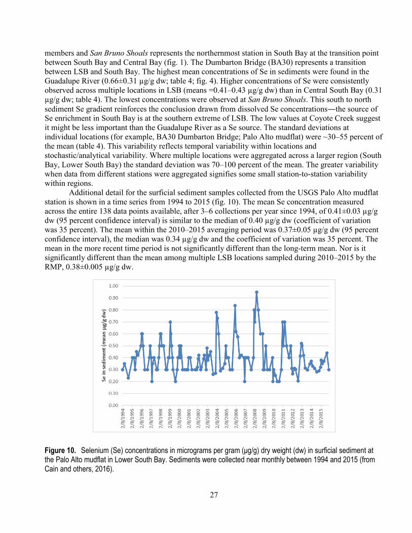
27

members and San Bruno Shoals represents the northernmost station in South Bay at the transition point between South Bay and Central Bay (fig. 1). The Dumbarton Bridge (BA30) represents a transition between LSB and South Bay. The highest mean concentrations of Se in sediments were found in the Guadalupe River (0.66±0.31 µg/g dw; table 4; fig. 4). Higher concentrations of Se were consistently observed across multiple locations in LSB (means =0.41–0.43 µg/g dw) than in Central South Bay (0.31 µg/g dw; table 4). The lowest concentrations were observed at San Bruno Shoals. This south to north sediment Se gradient reinforces the conclusion drawn from dissolved Se concentrations—the source of Se enrichment in South Bay is at the southern extreme of LSB. The low values at Coyote Creek suggest it might be less important than the Guadalupe River as a Se source. The standard deviations at individual locations (for example, BA30 Dumbarton Bridge; Palo Alto mudflat) were ~30–55 percent of the mean (table 4). This variability reflects temporal variability within locations and stochastic/analytical variability. Where multiple locations were aggregated across a larger region (South Bay, Lower South Bay) the standard deviation was 70–100 percent of the mean. The greater variability when data from different stations were aggregated signifies some small station-to-station variability within regions.

Additional detail for the surficial sediment samples collected from the USGS Palo Alto mudflat station is shown in a time series from 1994 to 2015 (fig. 10). The mean Se concentration measured across the entire 138 data points available, after 3–6 collections per year since 1994, of 0.41±0.03 µg/g dw (95 percent confidence interval) is similar to the median of 0.40 µg/g dw (coefficient of variation was 35 percent). The mean within the 2010–2015 averaging period was 0.37±0.05 µg/g dw (95 percent confidence interval), the median was 0.34 µg/g dw and the coefficient of variation was 35 percent. The mean in the more recent time period is not significantly different than the long-term mean. Nor is it significantly different than the mean among multiple LSB locations sampled during 2010–2015 by the RMP, 0.38±0.005 µg/g dw.

Figure 10. Selenium (Se) concentrations in micrograms per gram (μg/g) dry weight (dw) in surficial sediment at the Palo Alto mudflat in Lower South Bay. Sediments were collected near monthly between 1994 and 2015 (from Cain and others, 2016).

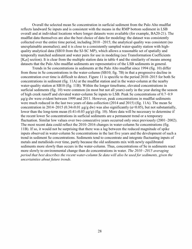
28

Overall the selected mean Se concentration in surficial sediment from the Palo Alto mudflat reflects landward Se inputs and is consistent with the means in the RMP bottom sediment in LSB overall and at individual locations where longer datasets were available (for example, BA20-21). The mudflat data themselves are also the best choice of data for modeling: the dataset was consistently collected over the entire time period, including 2010 –2015; the analytical quality was consistent (no unexplainable anomalies); and it is close to a consistently sampled water-quality station with high-quality analytical data (SB10 from the SJ-SC MP), which allows a reasonable set of spatially and temporally matched sediment and water pairs for use in modeling (see Transformation Coefficients [Kds] section). It is clear from the multiple station data in table 4 and the similarity of means among datasets that the Palo Alto mudflat sediments are representative of the LSB sediments in general.

Trends in Se concentrations in sediments at the Palo Alto mudflat since 1994 (fig. 10) differ from those in Se concentrations in the water-column (SB10; fig. 7B) in that a progressive decline in concentration over time is difficult to detect. Figure 11 is specific to the period 2010–2015 for both Se concentrations in sediment (fig. 11A) at the mudflat station and in the water-column at the nearby water-quality station at SB10 (fig. 11B). Within the longer timeframe, elevated concentrations in surficial sediments (fig. 10) were common (in most but not all years) early in the year during the season of high creek runoff and elevated water-column Se inputs to LSB. Peak Se concentrations of 0.7–0.9 µg/g dw were evident between 1999 and 2011. However, peak concentrations in mudflat sediments were much reduced in the last two years of data collection (2014 and 2015) (fig. 11A). The mean Se concentration in 2014–2015 (0.34±0.01 µg/g dw) was also significantly (ɑ<0.05), but not substantially, lower than the long-term mean (0.41±0.03 µg/g) (fig. 10). More data will be necessary to determine if the recent lower Se concentrations in surficial sediments are a permanent trend or a temporary fluctuation. Similar low values over two consecutive years occurred only once previously (2001–2002). The most recent data could reflect the 2010–2016 changes in water-column Se concentrations (fig. 11B). If so, it would not be surprising that there was a lag between the reduced magnitude of spike inputs observed in water-column Se concentrations in the last five years and the development of such a trend in sediment Se concentrations. Sediments tend to concentrate and integrate fluctuating inputs of metals and metalloids over time, partly because the old sediments mix with newly equilibrated sediments more slowly than occurs in the water-column. Thus, concentrations of Se in sediments react more slowly to environmental change than do concentrations in water. The 2010 –2015 averaging period that best describes the recent water-column Se data will also be used for sediments, given the uncertainties about future trends.

29

Figure 11. Selenium (Se) concentrations in micrograms per gram (μg/g) dry weight (dw) in A, surficial sediment at the Palo Alto mudflat for the period 2010-2015, and B, the water-column at nearby SB10 for the period 2010–2016. Concentrations peak early in the year in each year but peaks are much reduced in 2014 and 2015. Sediment samples were collected six times per year and water samples four times per year. Data: Cain and others, 2016; EPA, Region 9 data-file.

30

Selenium Concentrations in South Bay Invertebrates Data on Se concentrations in the invertebrates of LSB, to date, are limited to composite samples

of transplanted bivalves (for example, mussel: Mytilus californianus; oyster: Crassostrea gigas) collected by the RMP (http://cd3.sfei.org/) and a robust time series from the Palo Alto mudflat of Se concentrations in the resident bivalve M. petalum (previously M. balthica) collected by the USGS (see Supplemental References and especially Cain and others, 2016). In the RMP studies, mussels from Bodega Bay and oysters from Tomales Bay were transplanted in bags to three locations in South Bay, then recollected after 90 days of exposure (San Francisco Estuary Institute, 2017). At least one sample was collected every year from 1994 until 2001 and then again in 2008 and 2014. Over the entire data collection period, mean Se concentrations in reference-site bivalves were M. californiaus, 2.9 µg/g dw and C. gigas, 2.6 µg/g dw. The study locations in South Bay were Coyote Creek in LSB, the Dumbarton Bridge at the mouth of LSB, and Redwood Creek in Central South Bay. The greatest uncertainty with these data is that environmental conditions can greatly affect whether the animals will feed while in the bags. This is very important because food is overwhelmingly the primary source of Se uptake. If the animals do not feed they will not reflect Se concentrations in the environment to which they were transplanted. It is also difficult to tell if and how much they have fed. There is no obvious year-to-year trend in the Se uptake by the mussels at any site, although the small number of samples in the later years would make temporal trends difficult to detect even if the animals were feeding normally. Mean concentrations in sampled bivalves over the entire time series by location show Se concentrations in bivalves of 4.7±0.5 µg/g (standard error of the mean [SEM]) dw at Coyote Creek, 3.0±0.2 µg/g SEM dw at the Dumbarton Bridge, and 3.0±0.2 µg/g SEM dw at Redwood Creek. These means could reflect the spatial gradient in Se concentrations observed in water and sediment, with higher concentrations in LSB than in Central South Bay, but caution is advised for a quantitative conclusion because of 1) feeding issues associated with transplanted clams; and 2) the relatively small changes seem among sites and when compared to reference concentrations. Again these data point toward the conclusion that LSB is the region of greatest interest with regard to Se, and that the source(s) of elevated Se in South Bay are input(s) to LSB.

The most robust invertebrate data available from LSB are Se concentrations in the indicator clam, M. petalum (Cain and others, 2016). Selenium concentrations were determined in the soft tissue of this species using samples collected three to six times per year (normally in January, February, April, June, September, and December) since 1994. Approximately 40 clams were selected from an overall collected set of 60–120 individuals to achieve a range of sizes that were then split by clam size into three to six composite samples for analysis. Although clam size can be a factor affecting Se concentration (Strong and Luoma, 1981; Stewart and others, 2013), this long-term mudflat study also included biologic response measures such as condition index (that is, the relation of clam shell length and soft tissue weight; appendix fig. A4) that helped to understand the overall health and productivity of the benthic community. In our focused assessment of Se data here, a mean and SEM) were calculated for each date. Overall, analyses from 100 dates provide sufficient data from which to develop the model.

M. petalum can be considered a keystone species in South Bay and LSB. It is consistently present, and often abundant, in soft sediments. It is one of the ten most abundant benthic invertebrates in LSB. It also is one of the larger, if not the largest, abundant benthic invertebrate in LSB. Many of the species that are among the ten most abundant are quite small (appendix table A1), which affects their usefulness as both a food source for predators and as a Se indicator organism. Numerous publications have documented the usefulness of M. petalum as an indicator of metal and metalloid contamination in San Francisco Bay (Luoma and Cain, 1979; Thomson and others, 1984; Cain and Luoma, 1985, 1986,

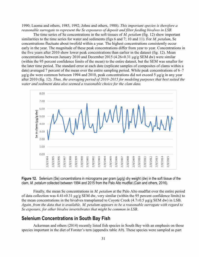
31

1990; Luoma and others, 1985, 1992; Johns and others, 1988). This important species is therefore a reasonable surrogate to represent the Se exposures of deposit and filter feeding bivalves in LSB.

The time series of Se concentrations in the soft tissues of M. petalum (fig. 12) show important similarities to the time series for water and sediments (figs 6 and 7; 10 and 11). For M. petalum, Se concentrations fluctuate about twofold within a year. The highest concentrations consistently occur early in the year. The magnitude of these peak concentrations differ from year to year. Concentrations in the five years after 2010 show lower peak concentrations than earlier in the dataset (fig. 12). Mean concentrations between January 2010 and December 2015 (4.26±0.31 µg/g SEM dw) were similar (within the 95 percent confidence limits of the mean) to the entire dataset, but the SEM was smaller for the later time period. The standard error at each date (replicate samples of composites of clams within a date) averaged 7 percent of the mean over the entire sampling period. While peak concentrations of 6–7 µg/g dw were common between 1994 and 2010, peak concentrations did not exceed 5 µg/g in any year after 2010 (fig. 12). Thus, the averaging period of 2010–2015 for modeling purposes that best suited the water and sediment data also seemed a reasonable choice for the clam data.

Figure 12. Selenium (Se) concentrations in micrograms per gram (μg/g) dry weight (dw) in the soft tissue of the clam, M. petalum collected between 1994 and 2015 from the Palo Alto mudflat (Cain and others, 2016).

Finally, the mean Se concentrations in M. petalum at the Palo Alto mudflat over the entire period of data collection was 4.41±0.31 µg/g SEM dw, very similar (within the 95 percent confidence limits) to the mean concentrations in the bivalves transplanted to Coyote Creek (4.7±0.5 µg/g SEM dw) in LSB. Again, from the data that is available, M. petalum appears to be a reasonable surrogate with regard to Se exposure, for other bivalve invertebrates that might be common in LSB.

Selenium Concentrations in South Bay Fish Ackerman and others (2014) recently listed fish species in South Bay with an emphasis on those

species important in the diet of Forster’s tern (appendix table A9). These species were sampled as part

32

of food-web components important to studies of Hg, but were not analyzed for tissue Se concentrations. Also listed in appendix table A9 is a subset of important predator species (see appendix tables A3 and A4 for a comprehensive listing). As stated in the South San Francisco Bay Ecosystem section above, white sturgeon is a species important both 1) to the derivation of the proposed San Francisco Bay and Delta Se criteria (U.S. Environmental Protection Agency, 2016b,c); and 2) in its connection to the endangered green sturgeon (U.S. Fish and Wildlife Service, 2009; https://ecos.fws.gov/ecp0/profile/speciesProfile?spcode=E087).

Only a few data for Se concentrations in fish from LSB are available. Benthic predators for which there are measurements of Se concentrations in muscle filets include white sturgeon and white croaker. Preparation of white croaker samples in 2014 included muscle with skin and skeleton (San Francisco Estuary Institute, 2003; http://cd3.sfei.org/). These samples were collected as part of long-term contaminant studies by the RMP (San Francisco Estuary Institute, 2003; http://cd3.sfei.org/). The mean Se concentration in 18 samples of white sturgeon muscle from 2009 and 2014 was 5.3±0.4 µg/g dw. The mean Se concentration in 13 samples of white croaker muscle for that period was 4.1±0.4 µg/g dw. The diet of both species include small fishes, shrimp, worms, small crabs, and clams, all of which reside in LSB. In locations where clams are abundant they can dominate the diet of sturgeon. Less is known about white croaker in San Francisco Bay. The only recent Se data for leopard shark were from three samples of muscle collected in 2009 where each sample was reported as containing 1.6 µg/g dw.

Selenium Concentrations in South Bay Birds Scattered data exist on Se concentrations in the eggs of some birds from San Francisco Bay.

Schwarzbach and others (2006) found a mean Se concentration of 2.1 µg/g dw in the eggs of Ridgway’s rail from four sloughs in South Bay (three of which were just south of the Dumbarton Bridge) in 1991–1992 (see also Lonzarich, 1992). This mean was similar to that for rail eggs (1.9 µg/g) at sites in North Bay for the same time period. Schwarzbach and Adelsman (2003) also reported on Se concentrations in the eggs of a variety of aquatic birds (table 5). The average concentration of Se in all eggs was 2.7 µg/g dw. Selenium concentrations ranged from 0.86 to 7.76 µg/g dw. The highest concentrations were in egret eggs. The mean concentration for Forster’s tern was 2.4 µg/g dw. The mean for California least tern was 2.8 µg/g dw.

Table 5. Mean selenium (Se) concentrations in micrograms per gram (μg/g) dry weight (dw) in the eggs of different species of aquatic birds from San Francisco Bay (Suisun and South Bay) collected in 2000. Exact locations for egg collections were not specified. Data: Schwarzbach and Adelsbach, 2003 (see Table 10). [n, number of samples]

Species Mean Se µg/g (dw) n1 SD Minimum Maximum 10th

percentile 90th

percentile Snowy plover (Charadrius

nivosus nivosus) 1.5 3 0.6 0.9 2.0 American avocet

(Recurvirostra Americana) 1.8 6 0.3 1.3 2.2 California clapper rail (Rallus

crepitans) 1.6 6 0.1 1.3 1.7 Brandt’s cormorant

(Phalacrocorax penicillatus ) 2.1 2 0.3 1.9 2.3 Forester’s tern (Sterna forsteri) 2.4 6 0.3 2.0 2.9 Black-necked stilt

(Himantopus mexicanus) 2.4 2 0.3 2.2 2.6 Double-crested cormorant

(Phalacrocorax auritus) 2.6 8 0.3 2.3 3.0

33

Species Mean Se µg/g (dw) n1 SD Minimum Maximum 10th

percentile 90th

percentile California least tern (Sternula

antillarum browni) 2.8 6 0.4 2.4 3.3 Black-crowned night heron

(Nycticorax nycticorax ) 3.5 11 0.7 2.5 4.6 2.6 4.3 Snowy egret (Egretta thula) 4.2 9 0.5 3.7 4.9 3.7 4.9 Great egret (Ardea alba) 3.0 15 1.4 2.0 7.8 2.0 3.4 All groups 2.8 74 1.1 0.9 7.8 1.7 4.2 1 If n=10, then percentiles are relevant.

Data for Se concentrations in livers of adult avocet, stilt, and Forster’s tern and their chicks are available as part of a study on body condition for these species at both North-, Central-, and South-Bay locations (Ackerman and Eagles-Smith, 2009). Although not directly relevant to criteria development, one finding here was that Se concentrations in livers of adult stilt and Forster’s tern in LSB were higher than in locations in Central and North Bay. For livers of chicks of avocets and stilts, Se concentrations were highest in LSB when compared to those in Central Bay.

The RMP collected more detailed data from LSB in 2009 and 2012. Samples of eggs (n=6–20) were collected from Forster’s tern nests in different ponds of the DENWR. Forster’s terns are fish-eating birds that nest in high densities at multiple sites within the salt ponds of South Bay and forage in both salt ponds and adjacent marshes (Ackerman and others, 2008a; 2009). Approximately 30 percent of the Forster’s terns breeding along the Pacific coast nest within San Francisco Bay, with salt ponds currently provide nesting habitat for 80 percent of these terns (Strong and others, 2004). Once Forster’s terns arrive in South Bay to breed, they use a relatively small area to forage and nest (Ackerman and others, 2008b; Bluso-Demers and others, 2008). Thus, Se concentrations in their eggs should reflect local food-web exposure, but from fish, not from benthic invertebrates that are subject to higher differential Se bioaccumulation (Presser and Luoma, 2010a).

Table 6 shows results of Se determinations in Forster’s tern eggs from different ponds in LSB. Among all data for 2009 and 2012, the mean Se concentration was 3.9 µg/g dw. Mean Se concentrations in each pond (table 6) show a declining gradient away from Alviso Slough/Guadalupe River (see fig. 4 for pond designations). The highest concentrations occur in the pond adjacent to Alviso Slough/Guadalupe River, concentrations then decline to the north. The differences between sites are small, but statistically significant (that is, 95 percent confidence limits do not overlap). This gradient is similar to that seen in water-column Se concentrations indicating, at a certain scale, that the most significant source of bioavailable Se in LSB originates from the Guadalupe River/Alviso Slough area.

Table 6. Mean selenium (Se) concentrations (± standard error of the mean [SEM]) in micrograms per gram (μg/g) dry weight (dw) in the eggs of Forster’s terns collected from several ponds in Lower South Bay in 2014. Sites are arranged spatially from east to west (that is, closer to Alviso Slough [mouth of the Guadalupe River] to further away from Alviso Slough [see map in fig. 4]). Forster’s Tern is a suitable indicator of spatial trends because of the species relatively small home territory, at least during some times of the year. Data: EPA, Region 9 data-file; SFEI RMP (http://cd3.sfei.org/)

Pond Location Se (µg/g) dw±SEM A7 Adjacent to Alviso Slough 4.3±0.03 AB2 West of A7 4.0±0.03 AB1 West of AB2 3.6±0.02 A2W West of AB1 3.3±0.03 A1 West of A2W 3.4±0.02

34

The RMP also sampled muscle of surf scoter (Melanitta perspicillata) and greater scaup (Aythya marila) as part of waterfowl consumption monitoring. Appendix fig. A5 shows Se concentrations in muscle of scoter and scaup (2002 and 2005) for a location north of the San Mateo Bridge (in South Bay) in comparison to scoter and scaup (2002) sampled from Suisun and San Pablo bays (in North Bay). Maximum Se concentrations at these locations are relatively comparable, an outcome that may reflect the foraging range of these species.

Presser-Luoma Ecosystem-Scale Selenium Model The data described above are adequate to employ the Presser-Luoma Ecosystem-Scale Selenium

Model to analyze Se issues in South Bay. As described by Presser and Luoma (2010a, 2010b, 2013), the model conceptualizes and quantifies the processes that determine how Se is transferred from water through diet to predators using trophic transfer factors (TTFs) and environmental transformation coefficients (Kds). The processes that influence the coefficients employed in the model include source loadings, speciation, transformation to primary producers, microbes and other forms of particulate material, bioaccumulation in invertebrates, and trophic transfer to predators. The modeling will link Se concentrations across water, particulate material, invertebrates, and tissues of different predator species in the LSB food web. Forecasts of bioaccumulation in predators can be linked to toxicity through tissue-based regulatory guidelines (U.S. Environmental Protection Agency, 2016a, 2016b). In the following sections the components and factors of the model will be developed, the resulting model will be validated, and then it will be used to translate desired Se concentration in fish tissue or the eggs of birds to a dissolved Se concentration that would be protective of these species in LSB.

The model illustrates some critical aspects of predicting site-and species-specific responses: • the choice of predator species determines the food web through which Se should be modeled; • the choice of food web is critical because Se bioaccumulation differs among prey (invertebrate)

species; • the concentration of Se associated with particulate material that is representative of the food of

the invertebrate employed in the model is used to quantify Se exposure to prey through the base of the food web; and

• the metric describing partitioning between particulate material and dissolved Se concentrations allows determination of a site-specific dissolved Se concentration that would be responsible for the concentration of Se in the chosen predator species that lives and feeds primarily in that specific environment.

Uncertainties and model sensitivities can be directly illustrated by varying exposure scenarios within a range typical of the site of interest. Thus, the model provides a tool to frame a site-specific ecological problem or occurrence of Se exposure and quantify exposure within that ecosystem.

The uncertainties in modeling are greatly influenced by the availability of site-specific data. Water, sediment, invertebrate, and fish data are the basic elements from which the model is developed. For LSB, the available data were described above. Time series for water-column Se concentrations are available from multiple sites. Time series for total Se concentrations in fine-grained surface sediments are available from one site as well as aggregated concentrations from multiple locations in LSB. Selenium concentrations in one of the predominant bivalves in the food web, M. petalum is available from one site. Selenium concentrations in benthic feeding fish and concentrations in the eggs of representative species of birds are available for comparison to model predictions (that is, validation). The model can be further calibrated by limiting choices of model coefficients (that is, TTFs and Kds) to those that best fit the field data as long as the former are consistent with mechanistic studies. If the model predictions and the field data are comparable (that is, the model is validated), then the model can

35

be used to calculate water-column Se concentrations that would be protective. The decisions as to the data to employ in the modeling, the validation, and any recalibration are documented in the following sections.

Chemical speciation data for Se are not available from LSB from either water or particulate material. The model can be run without such information. But interpretations of cause and effect (for example, why Kds differ from North Bay) would be more robust if such data were available. Similarly, Se concentrations in the food web at more locations and with more species would also facilitate interpretations. The existing data are sufficient to scope the problem in South Bay, but additional data would reduce uncertainties.

Transformation Coefficients (Kds) Connection to water-column Se concentrations in Ecosystem-Scale Selenium Modeling is

through transformation coefficients. The partitioning of Se between a water-column Se concentration and a particulate material Se concentration at the base of food webs is quantified using an operationally defined transformation coefficient, Kd, Kd = Sesediment/Sewater*1,000 (1) where Kd is defined as an instantaneous observed ratio that can capture, at a site-specific location, the intricacies of the biogeochemical processes that transform and control Se bioavailability across phases. At the core of the factor is quantifying the effects of dissolved Se speciation on uptake by organisms to produce bioavailable particulate material at the base of food webs that eventually helps drive food-web bioaccumulation and trophic transfer (Presser and Luoma, 2010a). It is important to specify what values for Sesediment and Sewater are used in equation 1 and to document the reasoning behind the choice of data. In South Bay this is especially important because multiple datasets are available from different sampling programs and locations.

With the Palo Alto mudflat time-series data, four approaches were compared to help justify and document the choice of Kd (table 7). First, Kds were calculated from Se concentrations that were collected on the same day from the Palo Alto mudflat (surficial sediment) and from the nearby SJ-SC MP station SB10 (water-column) (Approach a). Data are available from both these programs over the period 1993–2015. For the reasons defined above (changes in water-column concentrations over time) the primary period of interest is 2010–2015. Because these two programs were not coordinated in the timing of their samplings, and the SJ-SC MP reduced the frequency of sampling after 2010, same day sampling occurred in only seven instances within 2010–2015. Therefore, a second approach was employed (Approach b) in order to expand the dataset. In this case the same-day data were supplemented by including data from the first surficial sediment sampling after a water-column sampling when same-day sampling did not occur. There was no case where the period between samplings exceeded six weeks and in most cases it was less than a month. This expanded the 2010–2015 dataset from n=7 to n=21. Alternatively (Approach c), the mean Se concentrations in surficial sediment and in water for each year within the averaging period of 2010–2015 were used to calculate an annual mean Kd; then a grand mean Kd for the five years was calculated. Four water samples were taken per year in this period and six sediment samples per year.

36

Table 7. Comparison of four approaches in calculating transformation coefficient (Kd) for the Palo Alto mudflat station. Approach a calculated the mean Kd from only data collected on the same day for the period 2002–2016. Kds are compared for the periods 2002–2016 and 2010–2016. The latter was biased upward by a small dataset (n=7) and one high value that was greater than the 95th percentile value for the entire 2002–2016 dataset. Approach b expanded the dataset to include all water-column Se concentrations (collected 4 times per year) matched to the Se concentration of the next sediment sample collection after the date of the water-column collection. Approach c used the annual mean surficial sediment and water-column Se concentrations to calculate a grand mean for the period 2010–2016. Approach d calculated a mean Kd of the values from Approach b using those that were less than the 95th percentile and greater than the 5th percentile (that is, elimination of outliers). Data: Cain and others, 2016; see Supplementary References for complete list.

Approach

Description

Transformation Coefficient

(Kd±95% CI) a Same Day sampling—2002–2016 2,014±304 a Same Day sampling—2010–2016 2,863±1,002 b Same day plus closest coincidence 2010–2016 2,314±314 d1 Approach b for values <95th percentile and >5th percentile 2,016±183 c Grand mean of annual means: 2010–2016 2,022±210

1 Important to analysis and modeling in this report.

The primary goal in modeling was to use a Kd broadly typical of LSB. Hence, Approach d was used to test if a few exceptionally high or low values caused a bias by calculating mean Kds for the data that fell between the 5th percentile (eliminating lowest values) and the 95th percentile (eliminating highest values). Two of the 21 values were outside these limits for 2010–2015 and six of the 57 values were outside these limits for 2002–2010.

The outcomes of the four approaches showed that the highest Kd of 2,863 was that for the 2010–2015 period determined from the seven values from samples collected on exactly the same day (table 7). The confidence interval for this approach was ±50 percent. The large uncertainty, relative to other approaches, was caused by one value that was about four-times higher than the others (because of a very low water-column concentration). In general, amongst the other approaches, the mean Kds fell within the same band of confidence limits (the values were not significantly different at ɑ<0.05). The broader paired Kd was 2,016 when the exceptionally high and low values were eliminated; the annual means yielded a grand mean Kd of 2,022.

The Kd is typically the most variable of the coefficients in the Presser-Luoma Ecosystem-Scale Selenium Model. But the SEM was only 9–15 percent of the mean for Approaches b –d in LSB. The low variability characterized Kds for the entire sampling period. The mean Kd for the same day sampling for 2002–2015 was 2,014 within the 5th to 95th percentiles of the more restricted time period. The Kd for the entire dataset (1997–2015) was 2,019, similar to the 2010–2015 mean. For modeling the value 2,016 was chosen as most reasonable Kd to characterize the central tendency of the Palo Alto mudflat/SB10 data.

A second question is whether the Kd calculated from the Palo Alto mudflat/SB10 data is representative of LSB? It did not appear that bed sediment and water-column samples were collected simultaneously in time or space in the RMP program (see Selenium Concentrations in South Bay Waters and Sediments sections). But across all LSB locations sampled during 2010–2015, the Kd from the censored data was 1,645. At the one location (BA30 at the Dumbarton Bridge) where the RMP did collect both water-column and bed-sediment samples, the calculated mean Kd was 1,637. The mean Kd for Central South Bay when averaged across locations and time for 2010–2015 was 1,632. The spatial

37

agreement in Kds is remarkable. While the Kd from the Palo Alto mudflat/SB10 data was slightly higher than these (grand mean, 2,022±210; table 7), the values are within the same range. The slightly lower Kds from the RMP data could reflect coarser grain sizes (reducing sediment concentrations), as these sediments were not sieved. The finer grained (sieved) sediments are better representative of the grain sizes selected by M. petalum (Cain and Luoma, 1990) and of the fraction of sediments most likely to be suspended into the water-column by wind and tidal action. The Palo Alto mudflat/SB10 Kd will be used in the modeling. The Kd derived from the Palo Alto mudflat surficial sediments Se concentrations and the SJ-SC MP station SB10 water-column Se concentrations are generally representative of South Bay Se Kds. But we will test the sensitivity of model outcomes to the differences between RMP and Palo Alto-mudflat values.

Trophic Transfer Factors (TTFs) Trophic transfer factors are species-specific and link particulate material, invertebrate, and

predator Se concentrations. TTFs can be derived from field observations or can be determined experimentally in the laboratory (Presser and Luoma, 2010a).

Clam (M. petalum) Surficial sediment and clam data were collected concurrently from one site (Palo Alto mudflat)

in LSB since 1997. These data provide a robust set of data that can be used to calculate a field TTFclam for M. petalum where TTFM.petalum=[Se]M.petalum/[Se]sediment. (2) Selenium concentrations in both sediments and clams are subject to some stochastic variability and some seasonally consistent variability. For example, concentrations of metals such as copper and silver vary seasonally as condition index varies with the reproductive cycle (Cain and Luoma, 1990). The reproductive cycle has less influence on Se concentrations, but could be a small source of variability (Strong and Luoma, 1981; Stewart and others, 2013). TTFs can also be affected by:

• the type of food consumed by the clams; • changes in feeding rate; • lags between uptake and changes in Se concentrations in the environment; and • large differences in Se concentrations among considered sites.

Selenium concentrations in sediments can fluctuate with changes in particle size or source inputs into the environment.

Nevertheless, for most species of animals, there is a species-specific central tendency in TTFs that can be identified if statistical power (sample size) is adequate and the data range is not large. A distinct advantage of the dataset for the Palo Alto mudflat is the substantial amount of data (99 data points) from which TTFM. petalum can be calculated. Amongst all data (n = 99) the mean field TTFM. petalum at the Palo Alto mudflat was 12.3±0.5 SEM (fig. 13). Amongst the 2010–2015 data (n = 36) the mean was 13.0±0.9 SEM, partly driven by higher TTF’s in 2010. The two values were not significantly different. For all data, the 90th percentile value is 20.1 and the 10th percentile value is 7.3. Thus, the main body of the TTF data varies almost three-fold (fig. 13), but the 95 percent confidence interval for all data is only ±8 percent of the mean and for recent data is only ±14 percent of the mean (that is, there is little fluctuation around the mean TTFM. petalum). This signifies a low level of statistical uncertainty in estimating the mean value.

38

Figure 13. Calculated field trophic transfer factors (TTFs) for M. petalum between December 2009 and December 2015 at the Palo Alto mudflat.

Laboratory determinations of TTFM. petalum are a way to test if field observations are consistent with mechanistic explanations of trophic transfer. The availability of both kinds of data also addresses uncertainty about the validity of the chosen TTF. As explained by Luoma and Presser (2010a), TTFs are mechanistically defined partly from the assimilation efficiency (AE) of Se from a given food source, where AE is defined as the percentage of the Se within the food that is retained by the animal. Other contributors to the TTF are ingestion rate (IR) and the rate constant of Se loss (ke). All three have been defined experimentally for M. petalum. The simplified equation for calculating the tissue Se concentration (Cspecies) attributable to dietary exposure (Cfood) for a specific species (the extent of food-web Se bioaccumulation for that species) is Cspecies = [(AE) (IR) (Cf)]÷(ke) (3)

39

AEs can be variable with food type. M. petalum is a deposit feeder (feeds on surface sediments) and, less frequently, a suspension feeder (filters food particles from the water-column). Its digestive tract is designed to allow some separation of food rich particles like algal cells from inorganic materials of less nutritional value. Principle foods include detritus (decaying organic matter), living microbes, and plant cells (for example from diatom mats on the surface of sediment or filtered from the water-column) or a mixture of the three. In experiments that evaluated uptake from several different types of food, Luoma and others (1992) found Se AEs for M. petalum were 22 percent when the animals ingested largely anoxic sediments rich in elemental Se (the lowest bioavailability food source). While M. petalum can ingest subsurface sediments in which this form of Se would be dominant, it is not the usual way of feeding. AEs were as high as 86 percent when the animals ingested diatoms from a pure culture (Luoma and others, 1992). Schlekat and others (2000, 2004) found a mean AE of 78±7 percent when assimilation from five different kinds of algae was compared. AEs of oxic, detritus-rich suspended sediment in bivalves are between these two values (~45 percent; Wang and others, 1996). In nature, it would be likely that assimilation of Se from the mixed food entering the digestive tract of the clam would be a blend of the above values. Given the selectivity of the clam gut, the food assimilated is probably much richer in algae than in anaerobic sediment.

The kes varied from 0.012 to 0.030 in different experiments (summarized in Presser and Luoma 2010a). For modeling purposes a median ke of 0.021 was employed.

IRs by M. petalum varied from 0.25–1.0 g particulate per g tissue per day. Luoma and others (1992) employed an IR of 0.5 g sediment per g tissue per day based upon studies in the literature.

A reasonable range for TTFM. petalum, based on this combination of laboratory studies for this species, is 9–14 for different, but realistic, food sources and feeding rates (Presser and Luoma 2010a). Thus, the two field-derived mean TTFs (12.3 and 13.0) are very similar to the independently derived TTFs from laboratory studies. The variability in the field data, within the 10th to 90th percentiles, encompasses the range predicted from the laboratory. Thus, some of the variability in TTF in the field could reflect variability in food sources and feeding rates. Probably most important, the field derived TTFs were consistent with the mechanistically defined versions of TTF. For most modeling, a TTFM.

petalum of 12 was chosen (see additional discussion in Model Validation and Calibration of TTFs sections). This TTFM. petalum is similar to that observed in other bivalves that have been studied and, based upon field data, perhaps similar to invertebrate species like crabs or shrimp (Reinfelder and others, 1998).

Fish and Bird Species The generalized equations for calculation of species-specific TTFs derived from field data for

fish and birds are: TTFfish = [Se]fish/[Se]prey (4) or TTFbird egg = [Se]bird egg/[Se]prey (5) Experimental data, if available, can be used in the previously shown equation 3 to calculate mechanistic Se TTFs. Presser and Luoma (2010a) documented that both mechanistic and field-derived TTFs for whole-body fish varied less than 2 fold among species and that a value of 1.1 was reasonable for most species, so a whole-body TTFfish of 1.1 will be used in modeling scenarios. The U.S. Environmental Protection Agency (2016a) also provided a list of species-specific whole-body TTFs that has a mean whole-body TTFfish of 1.27.

40

Limited field data are available for deriving TTFs for bird eggs and development of mechanistic parameters has not been evaluated. For aquatic birds, the most data are available from controlled feeding of captive mallards (Anas platyrhynchos) exposed to known dietary Se concentrations (Heinz and others, 1989; Ohlendorf, 2003). TTFs calculated from matched data pairs for diet and bird egg tissue showed a range of TTFbird egg from 0.87 to 4.7. The mean TTFbird egg is 2.6. If dietary Se concentrations that are unrealistic for estuary food webs are eliminated (<1 μg/g dw and >18 μg/g dw), then a similar mean for TTFbird egg of 2.6 is calculated. A TTFbird egg of 2.6 is used here for modeling, which is the same value used in modeling for protection of North Bay bird species (U.S. Environmental Protection Agency, 2016b). Other approaches to derivation of wildlife criteria based on calculation of an allowable food concentration are also available (U.S. Fish and Wildlife Service, 2003; Presser and Luoma, 2010a). This data limitation may be addressed in the future if the EPA derives an approach and a national level of Se protection for wildlife, including aquatic dependent birds, or if further data becomes available on a species-specific basis.

Model Validation Validation answers the question: do all the pieces of the model, when combined, result in

predictions that are consistent with independent observations from the system? In other words, validation is defined by a comparison of the concentrations of Se predicted in organisms found in South Bay relative to the concentrations actually observed. It is also a way to evaluate the degree of uncertainty in the model. Several approaches were undertaken to validate the model for the LSB ecosystem. As noted earlier for M. petalum, the two field-derived mean TTFs (12.3 and 13.0; mean=12) were consistent with the range of mechanistically defined TTFs (9–14; median=10). The ranges overlapped and variability in food sources and feeding rates were postulated as reasons (see also: Calibration of TTFs section).

To test process consistency, Se concentrations in M. petalum were predicted for each date from the matched data employed in determining Kds for the 2010–2015 sampling period (table 8). The mean of the predictions for each day were then compared to mean Se concentrations observed in clams on those dates at the Palo Alto mudflat. To make the predictions, the mean field-derived Kd of 2,016 was employed and a TTFM. petalum of 12 was used. For the period 2010–2015, the predicted mean Se concentration in clams was 4.9±0.4 SEM and the observed mean concentration was 4.2±0.2 SEM (table 8). Thus, the combination of coefficients in the model generally captures the processes driving Se concentrations in M. petalum.

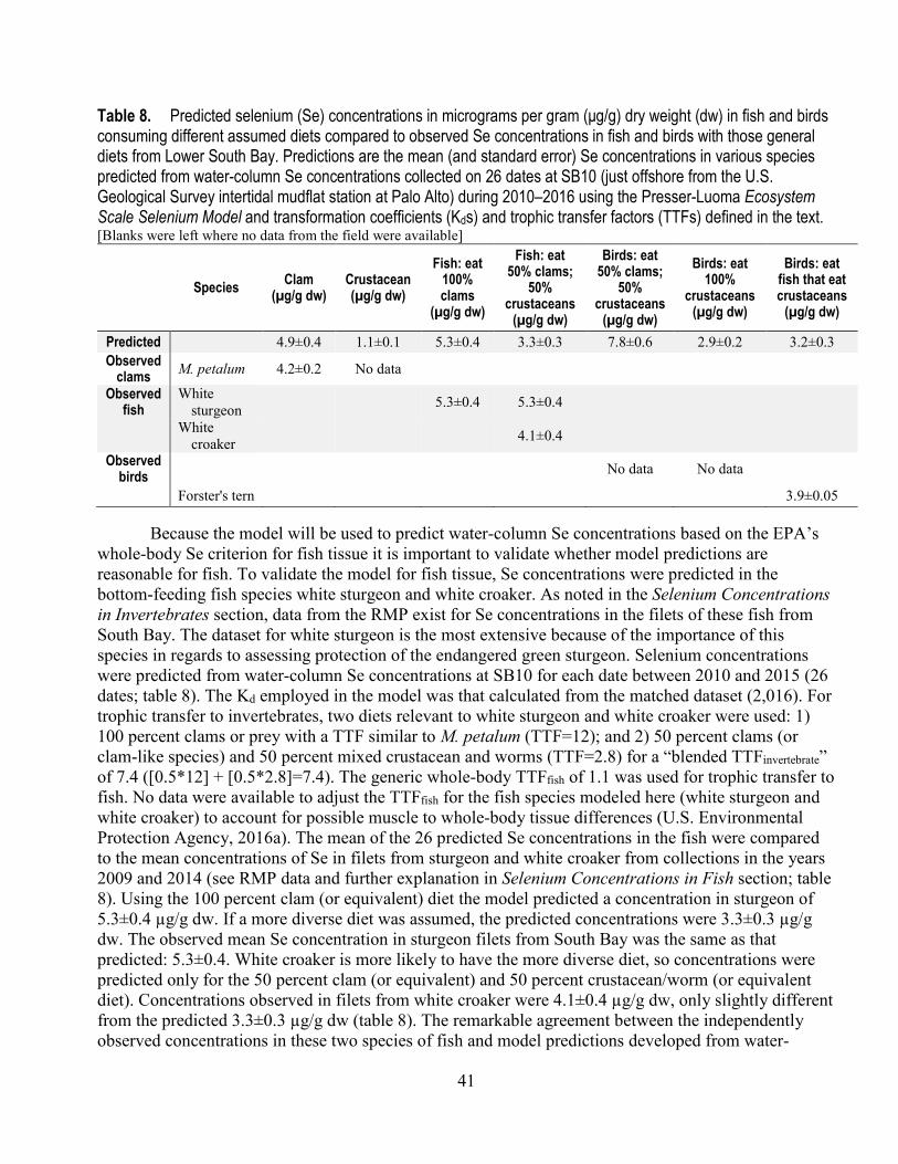
41

Table 8. Predicted selenium (Se) concentrations in micrograms per gram (μg/g) dry weight (dw) in fish and birds consuming different assumed diets compared to observed Se concentrations in fish and birds with those general diets from Lower South Bay. Predictions are the mean (and standard error) Se concentrations in various species predicted from water-column Se concentrations collected on 26 dates at SB10 (just offshore from the U.S. Geological Survey intertidal mudflat station at Palo Alto) during 2010–2016 using the Presser-Luoma Ecosystem Scale Selenium Model and transformation coefficients (Kds) and trophic transfer factors (TTFs) defined in the text. [Blanks were left where no data from the field were available]

Species Clam (µg/g dw)

Crustacean (µg/g dw)

Fish: eat 100% clams

(µg/g dw)

Fish: eat 50% clams;

50% crustaceans

(µg/g dw)

Birds: eat 50% clams;

50% crustaceans

(µg/g dw)

Birds: eat 100%

crustaceans (µg/g dw)

Birds: eat fish that eat crustaceans

(µg/g dw)

Predicted 4.9±0.4 1.1±0.1 5.3±0.4 3.3±0.3 7.8±0.6 2.9±0.2 3.2±0.3 Observed

clams M. petalum 4.2±0.2 No data

Observed fish

White sturgeon 5.3±0.4 5.3±0.4

White croaker 4.1±0.4

Observed birds No data No data

Forster's tern 3.9±0.05

Because the model will be used to predict water-column Se concentrations based on the EPA’s whole-body Se criterion for fish tissue it is important to validate whether model predictions are reasonable for fish. To validate the model for fish tissue, Se concentrations were predicted in the bottom-feeding fish species white sturgeon and white croaker. As noted in the Selenium Concentrations in Invertebrates section, data from the RMP exist for Se concentrations in the filets of these fish from South Bay. The dataset for white sturgeon is the most extensive because of the importance of this species in regards to assessing protection of the endangered green sturgeon. Selenium concentrations were predicted from water-column Se concentrations at SB10 for each date between 2010 and 2015 (26 dates; table 8). The Kd employed in the model was that calculated from the matched dataset (2,016). For trophic transfer to invertebrates, two diets relevant to white sturgeon and white croaker were used: 1) 100 percent clams or prey with a TTF similar to M. petalum (TTF=12); and 2) 50 percent clams (or clam-like species) and 50 percent mixed crustacean and worms (TTF=2.8) for a “blended TTFinvertebrate” of 7.4 ([0.5*12] + [0.5*2.8]=7.4). The generic whole-body TTFfish of 1.1 was used for trophic transfer to fish. No data were available to adjust the TTFfish for the fish species modeled here (white sturgeon and white croaker) to account for possible muscle to whole-body tissue differences (U.S. Environmental Protection Agency, 2016a). The mean of the 26 predicted Se concentrations in the fish were compared to the mean concentrations of Se in filets from sturgeon and white croaker from collections in the years 2009 and 2014 (see RMP data and further explanation in Selenium Concentrations in Fish section; table 8). Using the 100 percent clam (or equivalent) diet the model predicted a concentration in sturgeon of 5.3±0.4 µg/g dw. If a more diverse diet was assumed, the predicted concentrations were 3.3±0.3 µg/g dw. The observed mean Se concentration in sturgeon filets from South Bay was the same as that predicted: 5.3±0.4. White croaker is more likely to have the more diverse diet, so concentrations were predicted only for the 50 percent clam (or equivalent) and 50 percent crustacean/worm (or equivalent diet). Concentrations observed in filets from white croaker were 4.1±0.4 µg/g dw, only slightly different from the predicted 3.3±0.3 µg/g dw (table 8). The remarkable agreement between the independently observed concentrations in these two species of fish and model predictions developed from water-

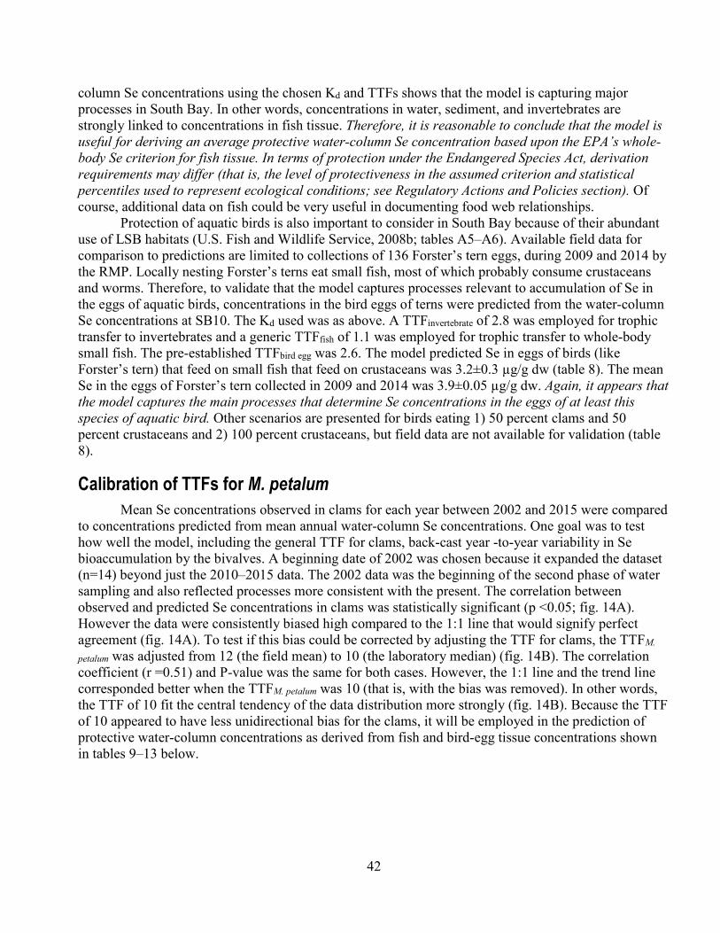
42

column Se concentrations using the chosen Kd and TTFs shows that the model is capturing major processes in South Bay. In other words, concentrations in water, sediment, and invertebrates are strongly linked to concentrations in fish tissue. Therefore, it is reasonable to conclude that the model is useful for deriving an average protective water-column Se concentration based upon the EPA’s whole-body Se criterion for fish tissue. In terms of protection under the Endangered Species Act, derivation requirements may differ (that is, the level of protectiveness in the assumed criterion and statistical percentiles used to represent ecological conditions; see Regulatory Actions and Policies section). Of course, additional data on fish could be very useful in documenting food web relationships.

Protection of aquatic birds is also important to consider in South Bay because of their abundant use of LSB habitats (U.S. Fish and Wildlife Service, 2008b; tables A5–A6). Available field data for comparison to predictions are limited to collections of 136 Forster’s tern eggs, during 2009 and 2014 by the RMP. Locally nesting Forster’s terns eat small fish, most of which probably consume crustaceans and worms. Therefore, to validate that the model captures processes relevant to accumulation of Se in the eggs of aquatic birds, concentrations in the bird eggs of terns were predicted from the water-column Se concentrations at SB10. The Kd used was as above. A TTFinvertebrate of 2.8 was employed for trophic transfer to invertebrates and a generic TTFfish of 1.1 was employed for trophic transfer to whole-body small fish. The pre-established TTFbird egg was 2.6. The model predicted Se in eggs of birds (like Forster’s tern) that feed on small fish that feed on crustaceans was 3.2±0.3 µg/g dw (table 8). The mean Se in the eggs of Forster’s tern collected in 2009 and 2014 was 3.9±0.05 µg/g dw. Again, it appears that the model captures the main processes that determine Se concentrations in the eggs of at least this species of aquatic bird. Other scenarios are presented for birds eating 1) 50 percent clams and 50 percent crustaceans and 2) 100 percent crustaceans, but field data are not available for validation (table 8).

Calibration of TTFs for M. petalum Mean Se concentrations observed in clams for each year between 2002 and 2015 were compared

to concentrations predicted from mean annual water-column Se concentrations. One goal was to test how well the model, including the general TTF for clams, back-cast year -to-year variability in Se bioaccumulation by the bivalves. A beginning date of 2002 was chosen because it expanded the dataset (n=14) beyond just the 2010–2015 data. The 2002 data was the beginning of the second phase of water sampling and also reflected processes more consistent with the present. The correlation between observed and predicted Se concentrations in clams was statistically significant (p <0.05; fig. 14A). However the data were consistently biased high compared to the 1:1 line that would signify perfect agreement (fig. 14A). To test if this bias could be corrected by adjusting the TTF for clams, the TTFM.

petalum was adjusted from 12 (the field mean) to 10 (the laboratory median) (fig. 14B). The correlation coefficient (r =0.51) and P-value was the same for both cases. However, the 1:1 line and the trend line corresponded better when the TTFM. petalum was 10 (that is, with the bias was removed). In other words, the TTF of 10 fit the central tendency of the data distribution more strongly (fig. 14B). Because the TTF of 10 appeared to have less unidirectional bias for the clams, it will be employed in the prediction of protective water-column concentrations as derived from fish and bird-egg tissue concentrations shown in tables 9–13 below.

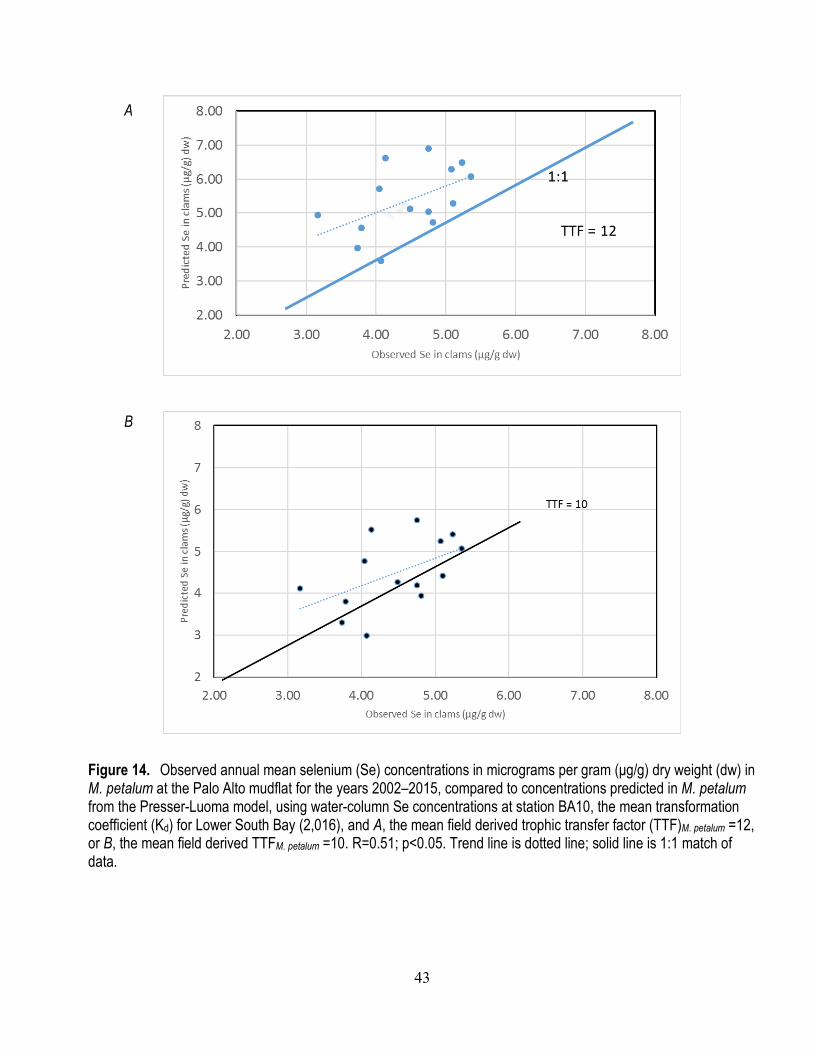
43

Figure 14. Observed annual mean selenium (Se) concentrations in micrograms per gram (μg/g) dry weight (dw) in M. petalum at the Palo Alto mudflat for the years 2002–2015, compared to concentrations predicted in M. petalum from the Presser-Luoma model, using water-column Se concentrations at station BA10, the mean transformation coefficient (Kd) for Lower South Bay (2,016), and A, the mean field derived trophic transfer factor (TTF)M. petalum =12, or B, the mean field derived TTFM. petalum =10. R=0.51; p<0.05. Trend line is dotted line; solid line is 1:1 match of data.

A

B

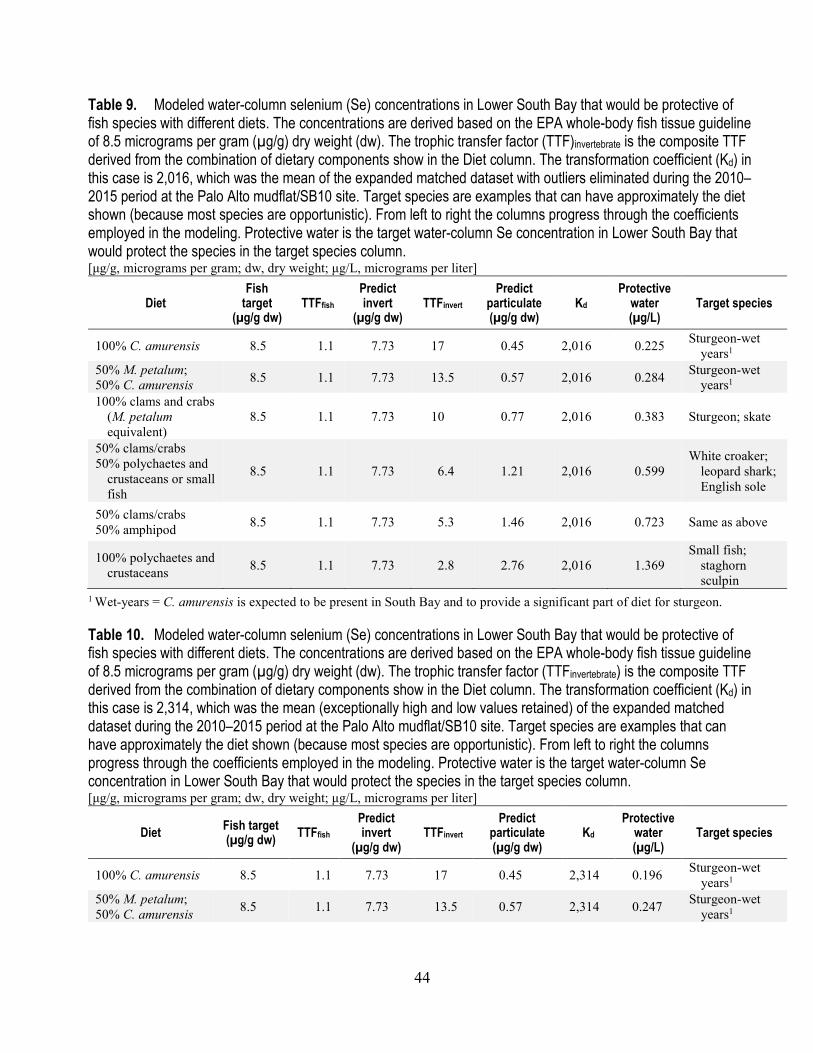
44

Table 9. Modeled water-column selenium (Se) concentrations in Lower South Bay that would be protective of fish species with different diets. The concentrations are derived based on the EPA whole-body fish tissue guideline of 8.5 micrograms per gram (µg/g) dry weight (dw). The trophic transfer factor (TTF)invertebrate is the composite TTF derived from the combination of dietary components show in the Diet column. The transformation coefficient (Kd) in this case is 2,016, which was the mean of the expanded matched dataset with outliers eliminated during the 2010–2015 period at the Palo Alto mudflat/SB10 site. Target species are examples that can have approximately the diet shown (because most species are opportunistic). From left to right the columns progress through the coefficients employed in the modeling. Protective water is the target water-column Se concentration in Lower South Bay that would protect the species in the target species column. [μg/g, micrograms per gram; dw, dry weight; μg/L, micrograms per liter]

Diet Fish target

(µg/g dw) TTFfish Predict invert

(µg/g dw) TTFinvert Predict particulate (µg/g dw) Kd Protective

water (µg/L) Target species

100% C. amurensis 8.5 1.1 7.73 17 0.45 2,016 0.225 Sturgeon-wet years1

50% M. petalum; 50% C. amurensis 8.5 1.1 7.73 13.5 0.57 2,016 0.284 Sturgeon-wet

years1 100% clams and crabs

(M. petalum equivalent) 8.5 1.1 7.73 10 0.77 2,016 0.383 Sturgeon; skate

50% clams/crabs 50% polychaetes and

crustaceans or small fish

8.5 1.1 7.73 6.4 1.21 2,016 0.599 White croaker;

leopard shark; English sole

50% clams/crabs 50% amphipod 8.5 1.1 7.73 5.3 1.46 2,016 0.723 Same as above

100% polychaetes and crustaceans 8.5 1.1 7.73 2.8 2.76 2,016 1.369

Small fish; staghorn sculpin

1 Wet-years = C. amurensis is expected to be present in South Bay and to provide a significant part of diet for sturgeon.

Table 10. Modeled water-column selenium (Se) concentrations in Lower South Bay that would be protective of fish species with different diets. The concentrations are derived based on the EPA whole-body fish tissue guideline of 8.5 micrograms per gram (µg/g) dry weight (dw). The trophic transfer factor (TTFinvertebrate) is the composite TTF derived from the combination of dietary components show in the Diet column. The transformation coefficient (Kd) in this case is 2,314, which was the mean (exceptionally high and low values retained) of the expanded matched dataset during the 2010–2015 period at the Palo Alto mudflat/SB10 site. Target species are examples that can have approximately the diet shown (because most species are opportunistic). From left to right the columns progress through the coefficients employed in the modeling. Protective water is the target water-column Se concentration in Lower South Bay that would protect the species in the target species column. [μg/g, micrograms per gram; dw, dry weight; μg/L, micrograms per liter]

Diet Fish target (µg/g dw) TTFfish

Predict invert

(µg/g dw) TTFinvert

Predict particulate (µg/g dw)

Kd Protective

water (µg/L)

Target species



years1

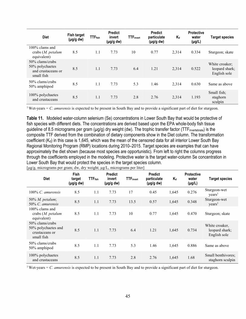
45

Diet Fish target (µg/g dw) TTFfish

Predict invert



Kd Protective

water (µg/L)

Target species

100% clams and crabs (M. petalum equivalent) 8.5 1.1 7.73 10 0.77 2,314 0.334 Sturgeon; skate

50% clams/crabs 50% polychaetes

and crustaceans or small fish

8.5 1.1 7.73 6.4 1.21 2,314 0.522 White croaker;


50% clams/crabs 50% amphipod 8.5 1.1 7.73 5.3 1.46 2,314 0.630 Same as above 100% polychaetes

and crustaceans 8.5 1.1 7.73 2.8 2.76 2,314 1.193 Small fish;

staghorn sculpin

1 Wet-years = C. amurensis is expected to be present in South Bay and to provide a significant part of diet for sturgeon.

Table 11. Modeled water-column selenium (Se) concentrations in Lower South Bay that would be protective of fish species with different diets. The concentrations are derived based upon the EPA whole-body fish tissue guideline of 8.5 micrograms per gram (µg/g) dry weight (dw). The trophic transfer factor (TTFinvertebrate) is the composite TTF derived from the combination of dietary components show in the Diet column. The transformation coefficient (Kd) in this case is 1,645, which was the mean of the censored data for all interior Lower South Bay Regional Monitoring Program (RMP) locations during 2010–2015. Target species are examples that can have approximately the diet shown (because most species are opportunistic). From left to right the columns progress through the coefficients employed in the modeling. Protective water is the target water-column Se concentration in Lower South Bay that would protect the species in the target species column. [μg/g, micrograms per gram; dw, dry weight; μg/L, micrograms per liter]

Diet Fish

target (µg/g dw)

TTFfish Predict invert



Kd Protective

water (µg/L)

Target species



years1 100% clams and

crabs (M. petalum equivalent) 8.5 1.1 7.73 10 0.77 1,645 0.470 Sturgeon; skate

50% clams/crabs 50% polychaetes and

crustaceans or small fish

8.5 1.1 7.73 6.4 1.21 1,645 0.734 White croaker,


50% clams/crabs 50% amphipod 8.5 1.1 7.73 5.3 1.46 1,645 0.886 Same as above

100% polychaetes and crustaceans 8.5 1.1 7.73 2.8 2.76 1,645 1.68 Small benthivores;

staghorn sculpin 1 Wet-years = C. amurensis is expected to be present in South Bay and to provide a significant part of diet for sturgeon.

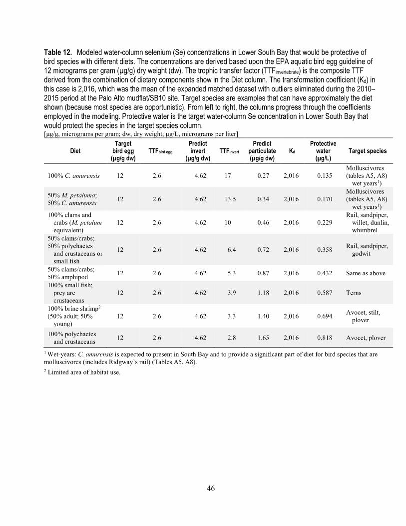
46

Table 12. Modeled water-column selenium (Se) concentrations in Lower South Bay that would be protective of bird species with different diets. The concentrations are derived based upon the EPA aquatic bird egg guideline of 12 micrograms per gram (µg/g) dry weight (dw). The trophic transfer factor (TTFinvertebrate) is the composite TTF derived from the combination of dietary components show in the Diet column. The transformation coefficient (Kd) in this case is 2,016, which was the mean of the expanded matched dataset with outliers eliminated during the 2010–2015 period at the Palo Alto mudflat/SB10 site. Target species are examples that can have approximately the diet shown (because most species are opportunistic). From left to right, the columns progress through the coefficients employed in the modeling. Protective water is the target water-column Se concentration in Lower South Bay that would protect the species in the target species column. [μg/g, micrograms per gram; dw, dry weight; μg/L, micrograms per liter]

Diet Target bird egg

(µg/g dw) TTFbird egg

Predict invert



100% C. amurensis 12 2.6 4.62 17 0.27 2,016 0.135 Molluscivores (tables A5, A8)

wet years1)

50% M. petaluma; 50% C. amurensis 12 2.6 4.62 13.5 0.34 2,016 0.170

Molluscivores (tables A5, A8)

wet years1) 100% clams and

crabs (M. petalum equivalent) 12 2.6 4.62 10 0.46 2,016 0.229

Rail, sandpiper, willet, dunlin, whimbrel

50% clams/crabs; 50% polychaetes


12 2.6 4.62 6.4 0.72 2,016 0.358 Rail, sandpiper, godwit

50% clams/crabs; 50% amphipod 12 2.6 4.62 5.3 0.87 2,016 0.432 Same as above

100% small fish; prey are crustaceans 12 2.6 4.62 3.9 1.18 2,016 0.587 Terns

100% brine shrimp2 (50% adult; 50%

young) 12 2.6 4.62 3.3 1.40 2,016 0.694 Avocet, stilt,

plover

100% polychaetes and crustaceans 12 2.6 4.62 2.8 1.65 2,016 0.818 Avocet, plover

1 Wet-years: C. amurensis is expected to present in South Bay and to provide a significant part of diet for bird species that are molluscivores (includes Ridgway’s rail) (Tables A5, A8). 2 Limited area of habitat use.

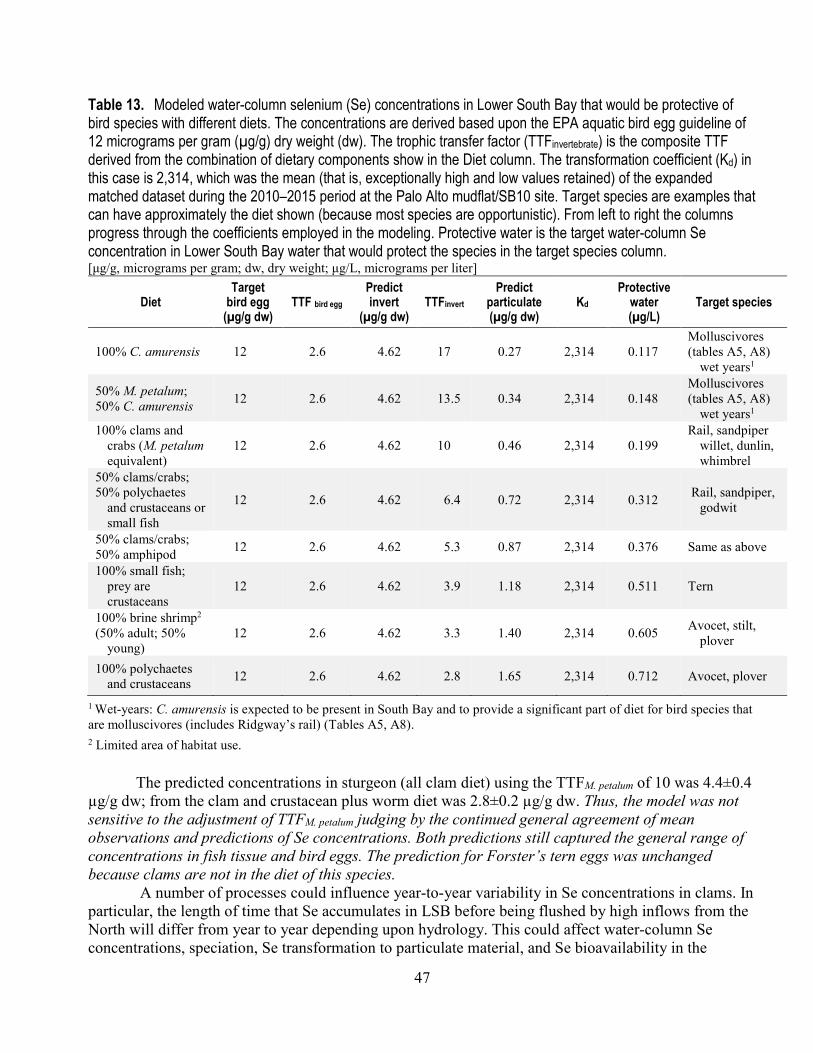
47

Table 13. Modeled water-column selenium (Se) concentrations in Lower South Bay that would be protective of bird species with different diets. The concentrations are derived based upon the EPA aquatic bird egg guideline of 12 micrograms per gram (µg/g) dry weight (dw). The trophic transfer factor (TTFinvertebrate) is the composite TTF derived from the combination of dietary components show in the Diet column. The transformation coefficient (Kd) in this case is 2,314, which was the mean (that is, exceptionally high and low values retained) of the expanded matched dataset during the 2010–2015 period at the Palo Alto mudflat/SB10 site. Target species are examples that can have approximately the diet shown (because most species are opportunistic). From left to right the columns progress through the coefficients employed in the modeling. Protective water is the target water-column Se concentration in Lower South Bay water that would protect the species in the target species column. [μg/g, micrograms per gram; dw, dry weight; μg/L, micrograms per liter]

Diet Target bird egg

(µg/g dw) TTF bird egg Predict invert



100% C. amurensis 12 2.6 4.62 17 0.27 2,314 0.117 Molluscivores (tables A5, A8)

wet years1 50% M. petalum; 50% C. amurensis 12 2.6 4.62 13.5 0.34 2,314 0.148

Molluscivores (tables A5, A8)

wet years1 100% clams and

crabs (M. petalum equivalent) 12 2.6 4.62 10 0.46 2,314 0.199

Rail, sandpiper willet, dunlin, whimbrel

50% clams/crabs; 50% polychaetes


12 2.6 4.62 6.4 0.72 2,314 0.312 Rail, sandpiper, godwit

50% clams/crabs; 50% amphipod 12 2.6 4.62 5.3 0.87 2,314 0.376 Same as above 100% small fish;

prey are crustaceans 12 2.6 4.62 3.9 1.18 2,314 0.511 Tern

100% brine shrimp2 (50% adult; 50%

young) 12 2.6 4.62 3.3 1.40 2,314 0.605 Avocet, stilt,

plover

100% polychaetes and crustaceans 12 2.6 4.62 2.8 1.65 2,314 0.712 Avocet, plover

1 Wet-years: C. amurensis is expected to be present in South Bay and to provide a significant part of diet for bird species that are molluscivores (includes Ridgway’s rail) (Tables A5, A8). 2 Limited area of habitat use.

The predicted concentrations in sturgeon (all clam diet) using the TTFM. petalum of 10 was 4.4±0.4 µg/g dw; from the clam and crustacean plus worm diet was 2.8±0.2 µg/g dw. Thus, the model was not sensitive to the adjustment of TTFM. petalum judging by the continued general agreement of mean observations and predictions of Se concentrations. Both predictions still captured the general range of concentrations in fish tissue and bird eggs. The prediction for Forster’s tern eggs was unchanged because clams are not in the diet of this species.

A number of processes could influence year-to-year variability in Se concentrations in clams. In particular, the length of time that Se accumulates in LSB before being flushed by high inflows from the North will differ from year to year depending upon hydrology. This could affect water-column Se concentrations, speciation, Se transformation to particulate material, and Se bioavailability in the

48

sediments. Nutrient inputs differ from year to year affecting primary producer uptake of Se (Crauder and others, 2016). The primary-producer species dominant in the food of benthos in LSB could change with inflows and nutrient concentrations. Clam growth could differ somewhat among years (Cain and others, 2016). And Se speciation could have changed over time as wetlands restoration progressed. Despite these potential uncertainties, the model captures the appropriate range of Se concentrations in clams, fish and birds both in terms of the long-term mean values and annual variability.

Water-Column Selenium Guidelines The Ecosystem-Scale Selenium Model can be used to determine potential protective water-

column criteria for Se using assumed tissue criteria for fish and birds and the equation: Cwater = Cpredator guideline ÷ (TTFpredator) (TTFinvertebrate) (Kd) (6)

This equation enables a site-specific translation of a regulatory or management tissue Se concentration (that is, an assumed Cfish or Cbird), once food-webs have been identified and model validation has taken place. The implications from a chosen tissue Se guidance can then readily be seen from the predicted increase or decrease from current conditions needed in dissolved Se concentrations and, eventually, in Se loading.

A set of site-specific scenarios and associated justified or derived food-web components and factors are given in tables 9–13. The modeling application for fish was initiated by employing the EPA’s national Se criterion for whole-body fish tissue of 8.5 µg/g dw that is designated as an EC 10 level of protection (U.S. Environmental Protection Agency, 2016a). Modeling for aquatic birds was initiated by employing the bird egg Se criterion proposed by the EPA for modeling of the North Bay (12 µg/g dw at a >EC20 level of protection; U.S. Environmental Protection Agency, 2016b, 2016c). In the main, Kds were developed from site SB10 (water-column) and the Palo Alto mudflat (surficial sediment) by approaches summarized for the time period 2010–2015 in table 7. As documented earlier, a Kd of 2,016 was chosen as most reasonable value to characterize the central tendency of the Palo Alto mudflat/SB10 data.

Fish Scenarios The North Bay water-column Se criterion for fish was based on the pathway of Se from water to

particulate material to C. amurensis to white sturgeon. C. amurensis is not typically abundant in South Bay. If sturgeon remains the fish species of regulatory interest, then M. petalum is the better choice of a surrogate for the sturgeon diet for this specific habitat. Using a Kd of 2,016, a TTFM. petalum of 10, and a generic whole-body TTFfish of 1.1, the model predicts a water-column Se concentration of 0.38 µg/L would be protective for South Bay (table 9). This assumes sturgeon feed almost entirely on bivalves like M. petalum or organisms with a similar TTFinvertebrate. For example, field data from North Bay suggest crabs bioaccumulate Se similarly to bivalves. This diet and guideline also would probably apply to the California skate (Rajidea inornata), a more abundant local fish predator that feeds on M. petalum and other bivalves.

In very wet years it is possible that C. amurensis could be more abundant. If the sturgeon diet were half M. petalum-like species (TTFM. petalum =10) and half C. amurensis (TTFC. amurensis =17), then 0.28 µg/L would be predicted as protective of sturgeon (table 9). However, this diet is unlikely in most years. White croaker is a fish species of interest because it is a benthic predator and is abundant in South Bay. If that species were consuming a diet of 50 percent clams/crabs (M. petalum equivalent) and 50 percent polychaetes, then 0.60 µg/L would be predicted as protective; but this would leave some risk to

49

any sturgeon visiting South Bay. Other diets and species are also shown in table 9 for the sake of illustration.

At the request of the EPA, an additional set of translations (table 10) was developed based on a somewhat higher Kd of 2,314 calculated by retaining the exceptionally high and low values of the 2010–2015 dataset (table 7). The set of comparable predicted protective Se concentrations derived for the diet scenarios described above would be 0.33, 0.25, and 0.52 µg/L.

The scenarios shown in tables 9 and 10 used Kds determined from the extensive dataset from one location: SB10 (water) and the Palo Alto mudflat (sediment). Table 11 tests the sensitivity of the predictions to a change in Kd of the order seen in LSB using the same set of dietary scenarios. In this case the Kd is 1,645, which was derived from the RMP sediment and mean SJ-SC MP water-column data for the interior of LSB. For the 100 percent M. petalum-like diet the predicted water-column Se concentration protective of sturgeon and similar clam-consuming species is 0.47 µg/L (table 11). The difference from the 0.38 µg/L prediction from the Palo Alto mudflat/SB10 dataset shows that the sensitivity to the range of Kds observed in LSB by different programs is small; in this case 0.09 µg/L or a 21 percent difference. The model outcomes for the Palo Alto mudflat/SB10 site are slightly more stringent for protection, but are representative of the larger area of LSB in general.

Bird Scenarios The water-column Se concentrations protective of the eggs of aquatic bird species are lower

overall than protections based upon fish species (tables 12 and 13). Reflective of restrictive cases for fish species (see table 9), bird species that eat 100 percent C. amurensis or 100 percent prey with a TTF similar to M. petalum would be protected by derived water-column Se concentrations of 0.14 or 0.23 µg/L, respectively (table 12). These derivations could be applicable to the locally nesting Ridgway’s rail or migratory shorebirds like sandpipers, willets, dunlins, and whimbrels that are classified as molluscivores (table 12). If a mixed diet of 50 percent clams/crabs (M. petalum equivalent) and 50 percent polychaetes, crustaceans, or amphipods is assumed for these species and other shorebird species that are considered crustaceavores or omnivores, then the range of derived protective water-column Se concentration is 0.36–0.43 µg/L. A concentration of 0.59 µg/L is predicted as protective of nesting terns that eat small fish (piscivores); and a concentration of 0.82 µg/L is predicted as protective of nesting plovers that eat a mix of bottom-dwelling polychaetes and crustaceans based on the regulated case. However, as noted previously, impacts to individuals in the case of endangered species (Ridgway’s rail, western snowy plover, and Forster’s tern) would need to be considered both in the analysis as well as in egg tissue guideline for an increased level of protection (see Regulatory Actions and Policies section).

For the requested set of translations (table 13) using the higher Kd of 2,314, the set of comparable predicted protective Se concentrations derived for the diet scenarios described above would be 0.20, 0.34, 0.32-0.38, 0.51, and 0.71 µg/L.

A scenario was also developed for the protection of American avocet, black-necked stilt, and western snowy plover that potentially could consume a diet of 100 percent brine shrimp in the limited area of extremely saline evaporation ponds. Under the lower Kd of 2,016, the protective concentration predicted using a mean TTFbrine shrimp for young and adult stages of 3.3, is 0.69 µg/L (table 12). Under the higher Kd of 2,314, the predicted protective guideline is 0.60 µg/L (table 13).

The Ecosystem-Scale Selenium Model, based on the regulated case where the ecosystem is generating 8.5 µg/g whole-body fish tissue and 12 µg/g bird eggs, predicts overall that slightly higher Se concentrations in the waters of South Bay than in North Bay would be protective for the species of birds and fish exposed to the highest dietary Se concentrations considered in the suite of food-web scenarios. A consistently lower and less variable Kd in South Bay and a food web that concentrates less Se than the

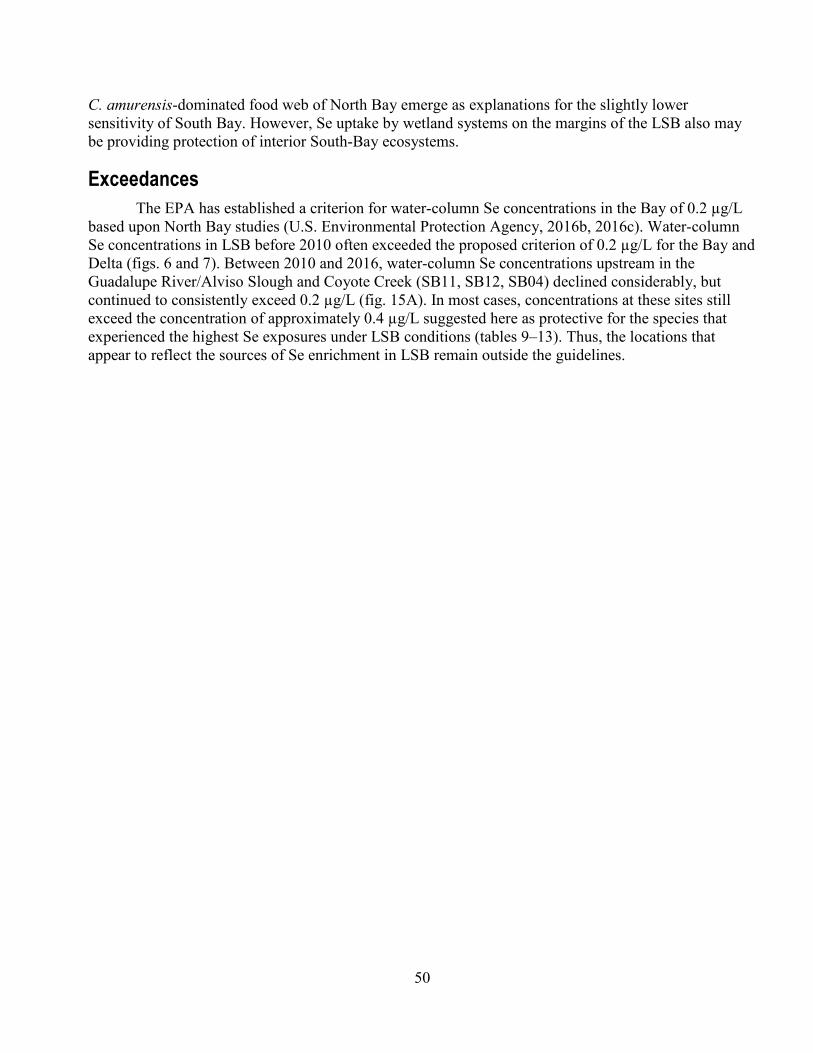
50

C. amurensis-dominated food web of North Bay emerge as explanations for the slightly lower sensitivity of South Bay. However, Se uptake by wetland systems on the margins of the LSB also may be providing protection of interior South-Bay ecosystems.

Exceedances The EPA has established a criterion for water-column Se concentrations in the Bay of 0.2 µg/L

based upon North Bay studies (U.S. Environmental Protection Agency, 2016b, 2016c). Water-column Se concentrations in LSB before 2010 often exceeded the proposed criterion of 0.2 µg/L for the Bay and Delta (figs. 6 and 7). Between 2010 and 2016, water-column Se concentrations upstream in the Guadalupe River/Alviso Slough and Coyote Creek (SB11, SB12, SB04) declined considerably, but continued to consistently exceed 0.2 µg/L (fig. 15A). In most cases, concentrations at these sites still exceed the concentration of approximately 0.4 µg/L suggested here as protective for the species that experienced the highest Se exposures under LSB conditions (tables 9–13). Thus, the locations that appear to reflect the sources of Se enrichment in LSB remain outside the guidelines.

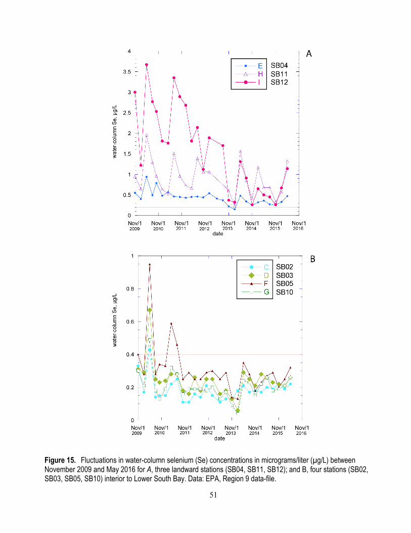
51

Figure 15. Fluctuations in water-column selenium (Se) concentrations in micrograms/liter (µg/L) between November 2009 and May 2016 for A, three landward stations (SB04, SB11, SB12); and B, four stations (SB02, SB03, SB05, SB10) interior to Lower South Bay. Data: EPA, Region 9 data-file.

52

In the interior of LSB, however, concentrations have also declined and are considerably lower than in the creeks (fig. 15B). Selenium concentrations at SB05, closest to the mouths of Guadalupe River/Alviso Slough and Coyote Creek, consistently exceeded a concentration of 0.2 µg/L during the 2010–2015 sampling period (fig. 15B). But seaward towards the Dumbarton Bridge, at the north end of LSB, exceedances are less common. For example, 69 percent of water-column Se concentrations at SB10 were ≥0.2 µg/L between 1994 and 2016 (appendix table A10). But exceedances fell to 42 percent of values at SB10 during the 2010–2015 sampling period (appendix table A11). After January 2011 no exceedances of water-column Se concentrations greater than 0.4 µg/L occurred at any of these four locations (fig. 15B).

Selenium concentrations in muscle filets of fish (white sturgeon, white croaker, leopard shark, jacksmelt (Atherinopsis californiensis), northern anchovy (Engraulis mordax), and shiner surfperch (Cymatogaster aggregata) collected from the Bay between 2009 and 2014 also rarely exceed the EPA whole-body Se criterion of 8.5 µg/g dw (U.S. Environmental Protection Agency, 2016a, 2016b, 2016c; figs. 16 and 17). Similarly, bird eggs of Forster’s tern and double-crested cormorant (Phalacrocorax auritus) do not exceed a 12 µg/g dw criterion (U.S. Environmental Protection Agency, 2016b, 2016c; fig. 18). The model would predict that fish tissues should generally be below 8.5 µg/g and bird eggs be below 12 µg/g in LSB and certainly this would be the case away from the major sources as in Central South Bay; and indeed that is the case. Again, the lower and more consistent Kd in South Bay is one explanation, reflecting a less efficient transformation of Se from water to particulates in South Bay than in North Bay.

53

Figure 16. Fish species' range of filet or ovary tissue selenium (Se) concentrations in micrograms per gram (µg/g) dry weight (dw) for 2009 and 2014 in South Bay. Whole, no head, tail, or guts (WNHTG). Data: EPA, Region 9 data-file; SFEI RMP (http://cd3.sfei.org).

54

Figure 17. White sturgeon filet selenium (Se) concentrations in micrograms per gram (µg/g) dry weight (dw) from 1997, 2000, 2003, 2006, 2009, and 2014 in South Bay. Data: EPA, Region 9 data-file; SFEI RMP (http://cd3.sfei.org).

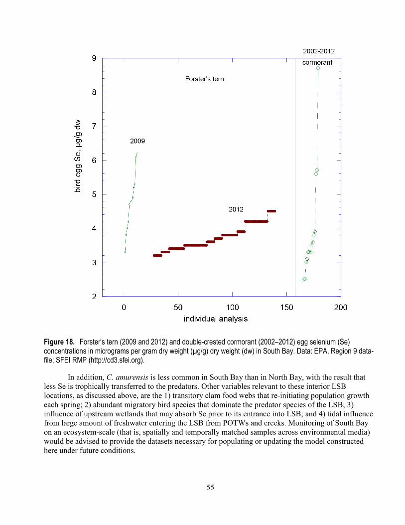
55

Figure 18. Forster's tern (2009 and 2012) and double-crested cormorant (2002–2012) egg selenium (Se) concentrations in micrograms per gram dry weight (µg/g) dry weight (dw) in South Bay. Data: EPA, Region 9 data-file; SFEI RMP (http://cd3.sfei.org).

In addition, C. amurensis is less common in South Bay than in North Bay, with the result that less Se is trophically transferred to the predators. Other variables relevant to these interior LSB locations, as discussed above, are the 1) transitory clam food webs that re-initiating population growth each spring; 2) abundant migratory bird species that dominate the predator species of the LSB; 3) influence of upstream wetlands that may absorb Se prior to its entrance into LSB; and 4) tidal influence from large amount of freshwater entering the LSB from POTWs and creeks. Monitoring of South Bay on an ecosystem-scale (that is, spatially and temporally matched samples across environmental media) would be advised to provide the datasets necessary for populating or updating the model constructed here under future conditions.

56

Conclusions Several questions were posed in the Introduction section to represent the goals of this study. The

analysis above shows that LSB is the source and the area of concern with regard to Se enrichment in South Bay. Although the most extensive dataset available for developing the model in LSB is from one location, that location is representative of LSB as a whole. Aqueous Se concentrations have declined substantially since the 1990s in LSB. Annual maximum Se concentrations have also declined in sediments and in the one bivalve species for which time-series data are available. As a result, the best averaging period for modeling LSB is the most recent period: 2010–2015.

The model assumes mean Kds and TTFs can be used to predict Se bioaccumulation in the food web of LSB from Se concentrations in sediment and water. The predictions from the Presser-Luoma Ecosystem-Scale Selenium Model closely match observations from LSB of Se concentrations in clams over time, concentrations in benthic-feeding fish, and concentrations in the eggs of one bird species for which extensive data is available, verifying that the model captures the general processes that control Se bioaccumulation in the LSB food webs. The match between observed and predicted concentrations is only weakly sensitive to different values for either Kd or for TTFs for bivalves. The range of aqueous Se concentrations that would be protective for LSB depends upon the species chosen for protection and the diet of those species, although the range for the most likely scenarios is relatively small (0.3–0.5 for fish; 0.2–0.4 for birds) (tables 9–13). In general, protective Se concentrations for LSB are slightly higher than those for North Bay because of a different food web in LSB and a lower and less variable Kd.

References Cited Ackerman, J.T., Bluso-Demers, J.D., and Takekawa, J.Y., 2009, Postfledging forster’s tern movements,

habitat selection, and colony attendance in San Francisco Bay: The Condor, v. 111, no. 1, p. 100–110. [Also available at https://doi.org/10.1525/cond.2009.080054.]

Ackerman, J.T., and Eagles-Smith, C.A., 2009, Selenium bioaccumulation and body condition in shorebirds and terns breeding in San Francisco Bay, California, USA: Environmental Toxicology and Chemistry, v. 28, no. 10, p. 2,134–2,141. [Also available at https://doi.org/10.1897/09-101.1.]

Ackerman, J.T., Eagles-Smith, C.A., Heinz, G.H., De La Cruz, S.E., Takekawa, J.Y., Miles, A.K., Adelsbach, T.L., Herzog, M.P., Bluso-Demers, J.D., Demers, S.A., Herring, G., Hoffman, D.J., Hartman, C.A., Willacker, J.J., Suchanek, T.H., Schwarzbach, S.E., and Maurer, T.C., 2014, Mercury in birds of San Francisco Bay-Delta, California—Trophic pathways, bioaccumulation, and ecotoxicological risk to avian reproduction: U.S. Geological Survey Open-File Report 2014-1251, 202 p., accessed May 30, 2018 at https://doi.org/10.3133/ofr20141251.

Ackerman, J.T., Eagles-Smith, C.A., Takekawa, J.Y., Bluso, J.D., and Adelsbach, T.L., 2008a, Mercury concentrations in blood and feathers of prebreeding forster’s terns in relation to space use of San Francisco Bay, California, USA, habitats: Environmental Toxicology and Chemistry, v. 27, no. 4, p. 897–908. [Also available at https://doi.org/10.1897/07-230.1.]

Ackerman, J.T., Eagles-Smith, C.A., Takekawa, J.Y., and Iverson, S.A., 2008b, Survival of post-fledging forster’s terns in relation to mercury exposure in San Francisco Bay: Ecotoxicology, v. 17, no. 8, p. 789–801. [Also available at https://doi.org/10.1007/s10646-008-0237-6.]

Amweg, E.L., Stuart, D.L., and Weston, D.P., 2003, Comparative bioavailability of selenium to aquatic organisms after biological treatment of agricultural drainage water: Aquatic Toxicology v. 63, no. 1, p. 13–25. [Also available at https://doi.org/10.1016/S0166-445X(02)00110-8.]

https://doi.org/10.1525/cond.2009.080054

57

Bay Area Stormwater Management Agencies Association, 2013, Selenium sub-report—Urban runoff characterization and control measures plan: Oakland, Calif., EOA Inc., 22 p.

Beller, E.E., Salomon, M., and Grossinger, R.M., 2013, An assessment of the south bay historical tidal-terrestrial transition zone: Oakland, Calif., San Francisco Estuary Institute (Publication 693), 20 p.

Bluso-Demers, J.D., Colwell, M.A., Takekawa, J.Y., and Ackerman, J.T., 2008, Space use by forster’s terns breeding in south San Francisco Bay: Waterbirds, v. 31, no. 3, p. 357–364. [Also available at https://doi.org/10.1675/1524-4695-31.3.357.]

Cain, D.J., and Luoma, S.N., 1985, Copper and silver accumulation in transplanted and resident clam (Macoma balthica) in south San Francisco Bay: Marine Environmental Research, v. 15, no. 2, p. 115–135. [Also available at https://doi.org/10.1016/0141-1136(85)90133-3.]

Cain, D.J., and Luoma, S.N., 1986, Effect of seasonally changing tissue weight on trace metal concentrations in the bivalve Macoma balthica in San Francisco Bay: Marine Ecology Progress Series, v. 28, no. 3, p. 209–217. [Also available at http://www.jstor.org/stable/24817437.]

Cain, D.J., and Luoma, S.N., 1990, Influence of seasonal growth, age, and environmental exposure on Cu and Ag in a bivalve indicator, Macoma balthica, in San Francisco Bay: Marine Ecology Progress Series, v. 60, no. 12, p. 45–55. [Also available at http://www.jstor.org/stable/24842576.]

Cain, D.J., Thompson, J.K., Crauder, J., Parchaso, F., Stewart, R., Turner, M.A., Hornberger, M.I., and Luoma, S.N., 2016, Near-field receiving water monitoring of trace metals and a benthic community near the Palo Alto Regional Water Quality Control Plant in south San Francisco Bay, California; 2015: U.S. Geological Survey Open-File Report 2016-1118, 78 p., accessed May 30, 2018 at https://doi.org/10.3133/ofr20161118.

California Regional Water Quality Control Board, San Francisco Bay Region, 2008, Guadalupe River watershed Mercury total maximum daily load (TMDL) project staff report for proposed basin plan amendment: Oakland, Calif., California Regional Water Quality Control Board, San Francisco Bay Region, 297 p.

[Also available at https://www.waterboards.ca.gov/sanfranciscobay/water_issues/programs/TMDLs/guadalupe_river_mercury/C1_Guad_SR_Sep08.pdf.]

California Regional Water Quality Control Board, San Francisco Bay Region, 2015, Permanente quarry and cement plant selenium impact assessment study—Final report for Lehigh Southwest Cement Company, Lehigh Facility, Cupertino, CA: Elk Grove, Calif., Robertson-Bryan, Inc., 86 p.

California Regional Water Quality Control Board, San Francisco Bay Region, 2014, Cease and desist order, Lehigh Southwest Cement Company and Hanson Permanente Cement, Inc., Permanente Plant: Oakland, Calif., California Regional Water Quality Control Board, San Francisco Bay Region, 15 p.

Cloern, J.E., 1991, Annual variations in river flow and primary production in the south San Francisco Bay estuary (USA), in Elliott, M., and Ducrotoy, J-P., eds., Estuaries and Coasts—Spatial and temporal intercomparisons: University of Caen, France, Olsen and Olsen, p. 91–96.

Cloern, J.E., Hieb, K.A., Jacobson, T., Sansó, B., Di Lorenzo, E., Stacey, M.T., Largier, J.L., Meiring, W., Peterson, W.T., Powell, T.M., Winder, M., and Jassby, A.D., 2010, Biological communities in San Francisco Bay track large-scale climate forcing over the North Pacific: Geophysical Research Letters, v. 37, no. 21, p. L21602 1-6. [Also available at https://doi.org/10.1029/2010GL044774.]

Cloern, J.E., Jassby, A.D., Thompson, J.K, and Hieb, K., 2007, A cold phase of the east Pacific triggers new phytoplankton blooms in San Francisco Bay: Proceedings of the National Academy of Science of the United States of America, v. 104, no. 47, p. 18,561–18,565. [Also available at https://doi.org/10.1073/pnas.0706151104.]

58

Conomos, T.J., 1979, Properties and circulation of San Francisco Bay waters, in Conomos, T.J., ed., San Francisco Bay—The urbanized estuary—Investigations into the natural history of San Francisco Bay and Delta with reference to the influence of man: San Francisco, Calif., Pacific Division American Association of the Advancement of Science, p. 47–84. [Also available at https://www.waterboards.ca.gov/waterrights/water_issues/programs/bay_delta/deltaflow/docs/exhibits/ccwd/spprt_docs/ccwd_conomos_1979.pdf.]

Crauder, J., Downing-Kunz, M.A., Hobbs, J.A., Manning, A.J., Novick, E., Parchaso, F., Wu, J., Schoellhamer, D.H., Senn, D.B., Shellenbarger, G.G., Thompson, J., and Yee, D., 2016, Lower south bay nutrient synthesis (contribution #732): Richmond, Calif., San Francisco Estuary Institute and the Aquatic Science Center, 227 p.

Davis, J.A., Yee, D., Collins, J.N., Schwarzbach, S.E., and Luoma, S.N., 2003, Potential for increased mercury accumulation in the estuary food web: San Francisco Estuary and Watershed Science, v. 1, no. 1, p. 1–36. [Also available at https://escholarship.org/uc/item/9fm1z1zb.]

De Graff, R.M., Tilghman, N.G., and Anderson, S.H., 1985, Foraging guilds of North American birds: Environmrntal Management, v. 9, no.6, p. 493–536. [Also available at https://doi.org/10.1007/BF01867324.]

Donehower, C., Scullen, J., and Tokatlian, K., 2013, Salt pond waterbird surveys data summary October 2011-September 2012: Milpitas, Calif., San Francisco Bay Bird Observatory, 66 p. [Also available at http://www.southbayrestoration.org/documents/technical/SFBBO%20Salt%20Pond%20Surveys%20Report%202012Revised-Mar-2013.pdf.]

East Bay Dischargers Authority, 2015, Sea level rise adaptation planning project—climate ready grant report: San Lorenzo, Calif., East Bay Dischargers Authority, 56 p.

Gallagher, M., and Brown, W.D., 1975, Composition of San Francisco Bay brine shrimp (Artemia salina): Journal of Agricultural and Food Chemistry, v. 23, no. 4, p. 630–632. [Also available at https://doi.org/10.1021/jf60200a008.]

Gross, E.S., Koseff, J.R., and Monismith, S.G., 1999, Three-dimensional salinity simulations of south San Francisco Bay: Journal of Hydraulic Engineering, v. 125, no. 11, p. 1,199–1,209. [Also available at https://doi.org/10.1061/(ASCE)0733-9429(1999)125:11(1199).]

Heinz, G.H., and Hoffman, D.J., 1998, Methymercury chloride and selenomethionine interactions on health and reproduction in mallards: Environmental Toxicology and Chemistry, v. 17, no. 2, p. 139–145. [Also available at https://doi.org/10.1002/etc.5620170202.]

Heinz, G.H., Hoffman, D.J., and Gold, L.G., 1989, Impaired reproduction of mallards fed an organic form of selenium: The Journal of Wildlife Management, v. 53, no. 2, p. 418–428. [Also available at https://doi.org/10.2307/3801145.]

Johns, C., Luoma, S.N., and Elrod, V., 1988, Selenium accumulation in benthic bivalves and fine sediments of San Francisco Bay, the Sacramento-San Joaquin Delta, and selected tributaries: Estuarine, Coastal, and Shelf Science, v. 27, no. 4, p. 381–396. [Also available at https://doi.org/10.1016/0272-7714(88)90095-9.]

Klimley, A.P., Chapman, E.D., Cech, J.J., Jr., Cocherell, D.E., Fangue, N.A., Gingras, M., Jackson, Z., Miller, E.A., Mora, E.A., Poletto, J.B., Schreier, A.M., Seesholtz, A., Sulak, K.J., Thomas, M.J., Woodbury, D., and Wyman, M.T., 2015, Sturgeon in the Sacramento-San Joaquin watershed—New insights to support conservation and management: San Francisco Estuary and Watershed Science, v. 13, no. 4, p. 1–21. [Also available at https://doi.org/10.15447/sfews.2015v13iss4art1.]

Lonzarich, D.G., Harvey, T.E., and Takekawa, J.E., 1992, Trace element and organochlorine concentrations in California clapper rail, (Rallus longirostris obsoletus) eggs: Archives of

59

Environmental Contamination and Toxicology, v. 23, no. 2, p. 147–153. [Also available at https://doi.org/10.1007/BF00212268.]

Luoma, S.N., and Cain, D.J., 1979, Fluctuations of copper, zinc, and silver in tellenid clams as related to freshwater discharge-south San Francisco Bay, in Conomos, T.J., ed., San Francisco Bay—The urbanized estuary—Investigations into the natural history of San Francisco Bay and Delta with reference to the influence of man: San Francisco, Calif., Pacific Division American Association of the Advancement of Science, p. 231–246. [Also available at https://www.waterboards.ca.gov/waterrights/water_issues/programs/bay_delta/deltaflow/docs/exhibits/ccwd/spprt_docs/ccwd_conomos_1979.pdf.]

Luoma, S.N., Cain, D.J., and Johansson, C., 1985, Temporal fluctuations of silver, copper and zinc in the bivalve Macoma balthica at five stations in south San Francisco Bay: Hydrobiologia, v. 129, no. 1, p. 109–120. [Also available at https://doi.org/10.1007/BF00048690.]

Luoma, S.N., Johns, C., Fisher, N.S., Steinberg, N.A., Oremland, R.S., and Reinfelder, J.R., 1992, Determination of selenium bioavailability to a benthic bivalve from particulate and solute pathways: Environmental Science and Technology, v. 26, no. 3, p. 485–491. [Also available at https://doi.org/10.1021/es00027a005.]

Luoma, S.N., and Presser, T.S., 2009, Emerging opportunities in management of selenium contamination: Environmental Science and Technology, v. 43, no. 22, p. 8,483–8,487. [Also available at https://doi.org/10.1021/es900828h.]

Luoma, S.N., and Rainbow, P.S., 2005, Why is metal bioaccumulation so variable? Biodynamics as a unifying concept: Environmental Science and Technology, v. 39, no. 7, p. 1,921–1,931. [Also available at https://doi.org/10.1021/es048947e.]

McKee, L.J., Bonnema, A., David, N., Davis, J.A., Franz, A., Grace, R., Greenfield, B.K., Gilbreath, A.N., Grosso, C., Heim, W.A., Hunt, J.A., Leatherbarrow, J.E., Lowe, S., Pearce, S.A., Ross, J.R.M., and Yee, D., 2017, Long-term variation in concentrations and mass loads in a semi-arid watershed influenced by historic mercury mining and urban pollutant sources: Science of the Total Environment, v. 605–606, p. 482–497. [Also available at https://doi.org/10.1016/j.scitotenv.2017.04.203.]

Melwani, A., and Thompson, B., 2007, The influence of chemical and physical factors on macrobenthos in the San Francisco Bay: Oakland, Calif., San Francisco Estuary Institute, 51 p.

Meseck, S., and Cutter, G., 2012, Selenium behavior in San Francisco Bay sediments: Estuaries and Coasts, v. 35, no. 2, p. 646–657. [Also available at https://doi.org/10.1007/s12237-011-9444-0.]

Nichols, F.H., and Pamatmat, M.M., 1988, The ecology of the soft-bottom benthos of San Francisco Bay—A community profile: U.S. Fish and Wildlife Service Biological Report 85(7.19), 73 p. [Also available at https://archive.usgs.gov/archive/sites/www.nwrc.usgs.gov/techrpt/85-7-23.pdf.]

Ohlendorf, H.M., 2003, Ecotoxicology of selenium, in Hoffman, D.J., Rattner, B.A., Burton, G.A., Jr, Cairns, J., Jr, eds, Handbook of ecotoxicology (2d ed.): Boca Raton, Fla., Lewis Publishers, p 465–500. Overton, C.T., Takekawa, J.Y., Casazza, M.L., Bui, T.D., Holyoak, M., and Strong, D.R., 2015, Sea-

level rise and refuge habitats for tidal marsh species—Can artificial islands save the California ridgway’s rail?: Ecological Engineering, v. 74, p. 337–344. [Also available at https://doi.org/10.1016/j.ecoleng.2014.10.016.]

Paganini, A., Kimmerer, W.J., and Stillman, J.H., 2010, Metabolic responses to environmental salinity in the invasive clam Corbula amurensis: Aquatic Biology, v.11, no.2, p. 139−147. [Also available at https://doi.org/10.3354/ab00304.]

Parchaso, F., Thompson, J.K., Crauder, J.S., Anduaga, R.I., and Pearson, S.A., 2015, Benthic response to water quality and biotic pressures in lower south San Francisco Bay, Alviso Slough, and Coyote

60

Creek: U.S. Geological Survey Open-File Report 2015-1234, 44p., accessed May 30, 2018 at https://doi.org/10.3133/ofr20151234.

Penglase, S., Hamre, K., and Ellingsen, S., 2014, Selenium and mercury have a synergistic negative effect on fish reproduction: Aquatic Toxicology, v. 149, p. 16–24. [Also available at https://doi.org/10.1016/j.aquatox.2014.01.020.]

Pitkin, M., and Wood, J., eds., 2011, The state of the birds San Francisco Bay: Petaluma, Calif., Point Reyes Bird Observatory Conservation Science and San Francisco Bay Joint Venture, 42 p. [Also available at http://data.prbo.org/sfstateofthebirds/.]

Presser, T.S., and Luoma, S.N., 2010a, A methodology for ecosystem-scale modeling of selenium: Integrated Environmental Assessment and Management, v. 6, no. 4, p. 685–710. [Also available at https://doi.org/10.1002/ieam.101.]

Presser, T.S., and Luoma, S.N., 2010b, Ecosystem-scale selenium modeling in support of fish and wildlife criteria development for the San Francisco Bay-Delta Estuary, California: U.S. Geological Survey Administrative Report, 101 p. and Appendices A-D, prepared for the U.S. Environmental Protection Agency, Region 9.

Presser, T.S., and Luoma, S.N., 2013, Ecosystem-scale selenium model for the San Francisco Bay-Delta Regional Ecosystem Restoration Implementation Plan (DRERIP): San Francisco Estuary and Watershed Science, v. 11, no. 1, p. 1–39. [Also available at https://escholarship.org/uc/item/2td0b99t.]

Presser, T.S., and Piper, D.Z., 1998, Mass balance approach to selenium cycling through the San Joaquin Valley—From source to river to bay, in Frankenberger, W.T., and Engberg, R.A., eds., Environmental chemistry of selenium: New York, Marcel Dekker, Inc, p. 153–182.

Reinfelder, J.R., Fisher, N.S., Luoma, S.N., Nichols, J.W., and Wang, W.-X., 1998, Trace element trophic transfer in aquatic organisms—A critique of the kinetic model approach: Science of the Total Environment, v. 219, no. 2–3, p. 117–135. [Also available at https://doi.org/10.1016/S0048-9697(98)00225-3.]

San Francisco Estuary Institute, 1995, Cruise report for Regional Monitoring Program—Water Sampling Cruise #17: Richmond, Calif., San Francisco Estuary Institute, 7 p.

San Francisco Estuary Institute, 1997, Cruise report for Regional Monitoring Program—Sediment Sampling Cruise #15: Richmond, Calif., San Francisco Estuary Institute, 9 p.

San Francisco Estuary Institute, 2003, Contaminant concentrations in fish from San Francisco Bay, 2000: Oakland Calif., San Francisco Estuary Institute, 82 p.

San Francisco Estuary Institute, 2015, Quality assurance program plan for the Regional Monitoring Program for water quality in San Francisco Bay: Richmond, Calif., San Francisco Estuary Institute, 154 p.

San Francisco Estuary Institute, 2017, Regional Monitoring Program field sampling report: Richmond, Calif., San Francisco Estuary Institute, 25 p.

San Jose-Santa Clara Regional Wastewater Facility, 2016, Annual self-monitoring report (NDPES Permit #CA-0037842): San Jose, Calif., San Jose-Santa Clara Regional Wastewater Facility, 57 p. [Also available at http://www.sanjoseca.gov/Archive.aspx?ADID=2950.]

Schlekat, C.E., Dowdle, P.R., Lee, B.-G., Luoma, S.N., and Oremland, R.S., 2000, Bioavailability of particle-associated Se to the bivalve Potamocorbula amurensis: Environmental Science and Technology, v. 34, no. 21, p. 4,504–4,510. [Also available at https://doi.org/10.1021/es001013f.]

Schlekat, C.E., Purkerson, D.G., and Luoma, S.N., 2004, Modeling selenium bioaccumulation through arthropod food webs in San Francisco Bay, California, USA: Environmental Toxicology and Chemistry, v. 23, no. 12, p. 3,003–3,010. [Also available at https://doi.org/10.1897/03-4.1.]

61

Schwarzbach, S.E., and Adelsbach, T., 2003, Assessment of ecological and human health impacts of mercury in the Bay-Delta watershed, CALFED Bay-Delta Mercury Project—Subtask 3b—Field assessment of avian mercury exposure in the Bay-Delta ecosystem: Sacramento, Calif., CALFED Bay-Delta Mercury Project, 29 p.

Schwarzbach, S.E., Albertson, J.D., and Thomas, C.M., 2006, Effects of predation, flooding and contamination on reproductive success of California Clapper Rails (Rallus longirostris obsoletus) in San Francisco Bay: The Auk. v. 123, no. 1, p. 45–60. [Also available at https://doi.org/10.1642/0004-8038(2006)123[0045:EOPFAC]2.0.CO;2.]

Skorupa, J.P., 1998, Selenium poisoning of fish and wildlife in nature—Lessons from twelve real-world examples, in Frankenberger, W.T., Jr., and Engberg, R.A., eds., Environmental Chemistry of Selenium: New York, Marcel Dekker Inc., p. 315–354.

Stewart, A.R., Luoma, S.N., Elrick, K.A., Carter, J.L., and van der Wegen, M., 2013, Influence of estuarine processes on spatiotemporal variation in bioavailable selenium: Marine Ecology Progress Series, v. 492, p. 41–56. [Also available at https://doi.org/10.3354/meps10503.]

Stewart, A.R., Luoma, S.N., Schlekat, C.E., Doblin, M.A., and Hieb, K.A., 2004, Food web pathway determines how selenium affects aquatic ecosystems—A San Francisco Bay case study: Environmental Science and Technology, v. 38, no. 17, p. 4,519–4,526. [Also available at https://doi.org/10.1021/es0499647.]

Strong, C.M., Spear, L.B., Ryan, T.P., and Dakin, R.E., 2004, Forster’s tern, caspian tern, and California gull colonies in San Francisco Bay—Habitat use, numbers and trends, 1982-2003: Waterbirds, v. 27, no. 4, p. 411–423. [Also available at https://doi.org/10.1675/1524-4695(2004)027[0411:FTCTAC]2.0.CO;2.]

Strong, C.R., and Luoma, S.N., 1981, Variations in correlation of body size with concentrations of Cu and Ag in the bivalve Macoma balthica: Canadian Journal of Fisheries and Aquatic Sciences, v. 38, no. 9, p. 1,059–1,064. [Also available at https://doi.org/10.1139/f81-146.]

Takekawa, J.Y., Lu, C.T., and Pratt, R.T., 2001, Avian communities in baylands and artificial salt evaporation ponds of the San Francisco Bay estuary, in Melack, J.M., Jellison, R., and Herbst, D.B., eds., Saline Lakes: Developments in Hydrobiology, v. 162, p. 317–328. [Also available at https://doi.org/10.1007/978-94-017-2934-5_29.]

Thomas, M.A., Conaway, C.H., Steding, D.J., Marvin-DiPasquale, M., Abu-Saba, K.E., and Flegal, A.R, 2002, Mercury contamination from historic mining in water and sediment, Guadalupe River and San Francisco Bay, California: Geochemistry: Exploration, Environment, Analysis, v. 2, no. 3, p. 211–217. [Also available at https://doi.org/10.1144/1467-787302-024.]

Thompson, B., Ranasinghe, J.A., Lowe, S., Melwani, A., and Weisberg, S.B., 2013, Benthic macrofaunal assemblages of the San Francisco Estuary and Delta, USA: Environmental Monitoring and Assessment, v. 185, no. 3, p. 2,281–2,295. [Also available at https://doi.org/10.1007/s10661-012-2708-8.]

Thompson, J.K., and Parchaso, F., 2012, Benthic invertebrate community assessment as a phytoplankton consumer and fish and bird prey source before and after start of the restoration: South Bay Salt Pond Restoration Project Cooperative Agreement #2009-0211, 90 p., accessed May 30, 2018 at http://www.southbayrestoration.org/documents/technical/Thompson%20Salt%20Pond%20 Complete%20Feb%202012.pdf.

Thompson, J.K., Koseff, J.R., Monismith, S.G., and Lucas, L.V., 2008, Shallow water processes govern system-wide phytoplankton bloom dynamics—A field study: Journal of Marine Systems, v. 74, no. 1–2, p. 153–166. [Also available at https://doi.org/10.1016/j.jmarsys.2007.12.006.]

http://www.southbayrestoration.org/documents/technical/Thompson%20Salt%20Pond

62

Thomson, E.A., Luoma, S.N., Johansson, C.E. and Cain, D.J., 1984, Comparison of sediments and organisms in identifying sources of biologically available trace metal contamination: Water Research, v. 18, no. 6, p. 756–765. [Also available at https://doi.org/10.1016/0043-1354(84)90172-6.]

U.S. Environmental Protection Agency, 2010, Expanded site inspection report—New Idria Mercury Mine, San Benito County, California (USEPA IAG 95777001-0 Region 9): Oakland, Calif., Weston Solutions Inc., 77 p.

U.S. Environmental Protection Agency, 2016a, Aquatic life ambient water quality criterion for selenium—Freshwater: Washington, D.C., U.S. Environmental Protection Agency, Office of Water, Office of Science and Technology, USEPA 822-R-16-006, 807 p., accessed May 30, 2018 at https://www.epa.gov/sites/production/files/2016-07/documents/aquatic_life_awqc_for_selenium_-_freshwater_2016.pdf.

U.S. Environmental Protection Agency, 2016b, Establishment of revised numeric criteria for selenium for the San Francisco Bay and Delta, State of California: Federal Register 7/15/2016, 13 p., accessed May 30, 2018 at https://www.gpo.gov/fdsys/pkg/FR-2016-07-15/pdf/2016-16266.pdf.

U.S. Environmental Protection Agency, 2016c, Technical Support Document for the Proposed Aquatic Life and Aquatic-Dependent Wildlife Selenium Water Quality Criteria for the San Francisco Bay and Delta: San Francisco, Calif., U.S. Environmental Protection Agency, Region 9, 100 p., accessed May 30, 2018 at https://www.regulations.gov/document?D=EPA-HQ-OW-2015-0392-0213.

U.S. Fish and Wildlife Service, 2003, Evaluation of the Clean Water Act section 304(a) human health criterion for methylmercury—Protectiveness for threatened and endangered wildlife in California: Sacramento, Calif., U.S. Fish and Wildlife Service, 112 p.

U.S. Fish and Wildlife Service, 2008a, Species at risk from selenium exposure in the San Francisco estuary: Sacramento, Calif., U.S. Fish and Wildlife Service, Sacramento Fish and Wildlife Office, 81 p., accessed May 30, 2018 at https://wwwrcamnl.wr.usgs.gov/Selenium/Library_articles/san_luis_articles/USFWS_Species_at_risk_from_Se_exposure_SF_Estuary_2008.pdf.

U.S. Fish and Wildlife Service, 2008b, Don Edwards San Francisco Bay National Wildlife Refuge bird list: Fremont, Calif., U.S. Fish and Wildlife Service, 9 p., accessed May 30, 2018 at https://www.fws.gov/uploadedFiles/DESFB_Bird%20List_2017.final.pdf.

U.S. Fish and Wildlife Service, 2009, Selenium effect levels for selected representative/surrogate species: Sacramento, Calif., U.S. Fish and Wildlife Service, 22 p.

U.S. Fish and Wildlife Service and California Department of Fish and Game, 2007, South bay salt pond restoration final environmental impact statement/report: Fremont, Calif., South Bay Salt Pond Restoration Project, EDAW, PW and Associates, HTH Associates, Brown and Caldwell, and Geomatrix, 57 p., accessed May 30, 2018 at http://www.southbayrestoration.org/EIR/downloads.html.

Walters, R.A., Cheng, R.T., and Conomos, T.J., 1985, Time scales of circulation and mixing processes of San Francisco Bay waters, in Cloern, J.E., and Nichols, F.H., eds., Temporal dynamics of an estuary—San Francisco Bay: Developments in Hydrobiology, v. 30, p. 13–36. [Also available at https://doi.org/10.1007/978-94-009-5528-8_2.]

Wang, W.-X., Fisher, N.S., and Luoma, S.N., 1996, Kinetic determinations of trace element bioaccumulation in the mussel Mytilus edulis: Marine Ecology Progress Series, v. 140, no. 1–3, p. 91–113. [Also available at http://www.jstor.org/stable/24857164.]

63

Supplementary References The following references contain datasets for Macoma petalum (previously Macoma balthica)

from 1997 through 2015. References are listed in chronological order for ease in locating data for a specific year. Luoma, S.N., Wellise, C., Cain, D.J., Brown, C., Hornberger, M., and Bouse, R., 1998, Near field

receiving water monitoring of trace metals in clams (Macoma balthica) and sediments near the Palo Alto and San Jose/Sunnyvale Water Quality Control Plants in south San Francisco Bay, 1997: U.S. Geological Survey Open-File Report 98-563, 88 p.

Wellise, C.J., Luoma, S.N., Cain, D.J., Brown, C., Hornberger, M., and Bouse, R., 1999, Near field receiving water monitoring of trace metals in clams (Macoma balthica) and sediments near the Palo Alto and San Jose/Sunnyvale Water Quality Control Plants in south San Francisco Bay (1998): U.S. Geological Survey Open-File Report 99-455, 101 p.

David, C.P.C, Luoma, S.N., Brown, C.L., Cain, D.J., Hornberger, M.I., and Lavigne, I.R., 2002, Near field receiving water monitoring of trace metals in clams (Macoma balthica) and sediments near the Palo Alto Water Quality Control Plant in south San Francisco Bay, California—1999–2001: U.S. Geological Survey Open-File Report 2002-453, 44 p., accessed May 30, 2018 at https://pubs.er.usgs.gov/publication/ofr02453.

Moon, E., David, C.P.C, Luoma, S.N., Cain, D.J., Hornberger, M.I., and I.R. Lavigne, 2003, Near field receiving water monitoring of trace metals in clams (Macoma balthica) and sediments near the Palo Alto Water Quality Control Plant in south San Francisco Bay—2002: U.S. Geological Survey Open-File Report 2003-339, 78 p., accessed May 30, 2018 at https://pubs.er.usgs.gov/publication/ofr03339.

Moon, E., Shouse, M.K., Parchaso, F., Thompson, J.K., Luoma, S.N., Cain, D.J., and Hornberger, M.I., 2005, Near-field receiving water monitoring of trace metals and a benthic community near the Palo Alto Regional Water Quality Control Plant in south San Francisco Bay, California—2004: U.S. Geological Survey Open-File Report 2005-1279, 118 p., accessed May 30, 2018 at https://pubs.er.usgs.gov/publication/ofr20051279.

Cain, D.J., Parchaso, F., Thompson, J.K., Luoma, S.N., Lorenzi, A.H., Moon, E., Shouse, M.K., Hornberger, M.I., and Dyke, J.L., 2006, Near-field receiving water monitoring of trace metals and a benthic community near the Palo Alto Regional Water Quality Control Plant in south San Francisco Bay, California—2005: U.S. Geological Survey Open-File Report 2006-1152, 120 p., [Also available at https://pubs.er.usgs.gov/publication/ofr20061152.]

Lorenzi, A.H., Cain, D.J., Parchaso, F., Thompson, J.K., Luoma, S.N., Hornberger, M.I., Dyke, J.L., Cervantes, R., and Shouse, M.K., 2007, Near-field receiving water monitoring of trace metals and a benthic community near the Palo Alto Regional Water Quality Control Plant in south San Francisco Bay, California—2006: U.S. Geological Survey Open-File Report 2007-1199, 118 p., accessed May 30, 2018 at https://pubs.er.usgs.gov/publication/ofr20071199.

Lorenzi, A.H., Cain, D.J., Parchaso, F., Thompson, J.K., Luoma, S.N., Hornberger, M.I., and Dyke, J.L., 2008, Near-field receiving water monitoring of trace metals and a benthic community near the Palo Alto Regional Water Quality Control Plant in south San Francisco Bay, California—2007: U.S. Geological Survey Open-File Report 2008-1180, 120 p., accessed May 30, 2018 at https://pubs.er.usgs.gov/publication/ofr20081180.

Cain, D.J., Thompson, J.K., Dyke, J.L. Parchaso, F., Luoma, S.N., and Hornberger, M.I., 2009, Near-field receiving water monitoring of trace metals and a benthic community near the Palo Alto Regional Water Quality Control Plant in south San Francisco Bay, California—2008: U.S. Geological Survey Open-File Report 2009-1193, 120p., accessed May 30, 2018 at https://pubs.er.usgs.gov/publication/ofr20091193.

64

Dyke, J.L., Parchaso, F., Thompson, J.K., Cain, D.J., Luoma, S.N., and Hornberger, M.I., 2010, Near-field receiving water monitoring of trace metals and a benthic community near the Palo Alto Regional Water Quality Control Plant in south San Francisco Bay, California—2009: U.S. Geological Survey Open-File Report 2010-1188, 46 p., accessed May 30, 2018 at https://pubs.er.usgs.gov/publication/ofr20101188.

Dyke, J.L., Parchaso, F., Thompson, J.K., Cain, D.J., Luoma, S.N., and Hornberger, M.I., 2011, Near-field receiving water monitoring of trace metals and a benthic community near the Palo Alto Regional Water Quality Control Plant in south San Francisco Bay, California—2010: U.S. Geological Survey Open-File Report 2011-1163, 24 p., accessed May 30, 2018 at https://pubs.er.usgs.gov/publication/ofr20111163.

Dyke, J.L., Thompson, J.K., Cain, D.J., Kleckner, A.E., Parchaso, F., Luoma, S.N., and Hornberger, M.I., 2012, Near-field receiving water monitoring of trace metals and a benthic community near the Palo Alto Regional Water Quality Control Plant in south San Francisco Bay, California—2011: U.S. Geological Survey Open-File Report 2012-1165, 108 p., accessed May 30, 2018 at https://pubs.er.usgs.gov/publication/ofr20121165.

Dyke, J.L., Thompson, J.K., Cain, D.J., Kleckner, A.E., Parchaso, F., Luoma, S.N., and Hornberger, M.I., 2013, Near-field receiving water monitoring of trace metals and a benthic community near the Palo Alto Regional Water Quality Control Plant in south San Francisco Bay, California, 2012: U.S. Geological Survey Open-File Report 2013-1144, 109 p., accessed May 30, 2018 at https://pubs.er.usgs.gov/publication/ofr20131144.

Dyke, J.L., Cain, D.J., Thompson, J.K., Kleckner, A.E., Parchaso, F., Hornberger, M.I., and Luoma, S.N., 2014, Near-field receiving water monitoring of trace metals and a benthic community near the Palo Alto Regional Water Quality Control Plant in south San Francisco Bay, California—2013: U.S. Geological Survey Open-File Report 2014-1174, 81 p., accessed May 30, 2018 at

https://doi.org/10.3133/ofr20141174. Cain, D.J., Thompson, J.K., Crauder, J.S., Parchaso, F., Stewart, A.R., Kleckner, A.E., Dyke, J.L.,

Hornberger, M.I., and Luoma, S.N., 2015, Near-field receiving water monitoring of trace metals and a benthic community near the Palo Alto regional water quality control plant in south San Francisco Bay, California, 2014: U.S. Geological Survey Open-File Report 2015-1199, 79 p., accessed May 30, 2018 at https://doi.org/10.3133/ofr20151199.

Cain, D.J., Thompson, J.K., Crauder, J.S., Parchaso, F., Stewart, A.R., Turner, M.A., Hornberger, M.I., and Luoma, S.N., 2016, Near-field receiving water monitoring of trace metals and a benthic community near the Palo Alto Regional Water Quality Control Plant in south San Francisco Bay, California—2015: U.S. Geological Survey Open-File Report 2016-1118, 78 p., accessed May 15, 2018 at https://doi.org/10.3133/ofr20161118.

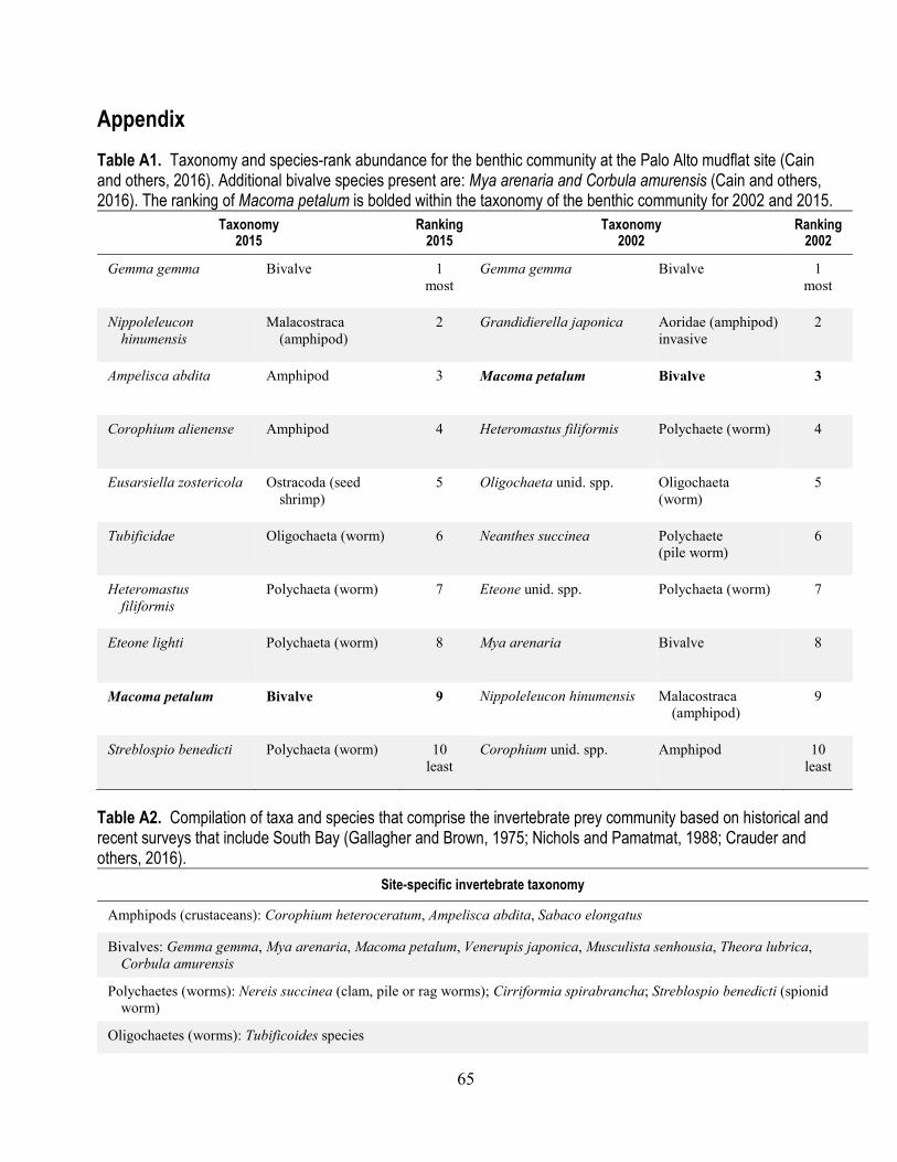
65

Appendix Table A1. Taxonomy and species-rank abundance for the benthic community at the Palo Alto mudflat site (Cain and others, 2016). Additional bivalve species present are: Mya arenaria and Corbula amurensis (Cain and others, 2016). The ranking of Macoma petalum is bolded within the taxonomy of the benthic community for 2002 and 2015.

Taxonomy 2015

Ranking 2015

Taxonomy 2002

Ranking 2002

Gemma gemma Bivalve 1 most

Gemma gemma Bivalve 1 most

Nippoleleucon hinumensis

Malacostraca (amphipod)

2 Grandidierella japonica Aoridae (amphipod) invasive

2

Ampelisca abdita Amphipod 3 Macoma petalum Bivalve 3

Corophium alienense Amphipod 4 Heteromastus filiformis Polychaete (worm) 4

Eusarsiella zostericola Ostracoda (seed shrimp)

5 Oligochaeta unid. spp. Oligochaeta (worm)

5

Tubificidae Oligochaeta (worm) 6 Neanthes succinea Polychaete (pile worm)

6

Heteromastus filiformis

Polychaeta (worm) 7 Eteone unid. spp. Polychaeta (worm) 7

Eteone lighti Polychaeta (worm) 8 Mya arenaria Bivalve 8

Macoma petalum Bivalve 9 Nippoleleucon hinumensis Malacostraca (amphipod)

9

Streblospio benedicti Polychaeta (worm) 10 least

Corophium unid. spp. Amphipod 10 least

Table A2. Compilation of taxa and species that comprise the invertebrate prey community based on historical and recent surveys that include South Bay (Gallagher and Brown, 1975; Nichols and Pamatmat, 1988; Crauder and others, 2016).

Site-specific invertebrate taxonomy

Amphipods (crustaceans): Corophium heteroceratum, Ampelisca abdita, Sabaco elongatus Bivalves: Gemma gemma, Mya arenaria, Macoma petalum, Venerupis japonica, Musculista senhousia, Theora lubrica,

Corbula amurensis Polychaetes (worms): Nereis succinea (clam, pile or rag worms); Cirriformia spirabrancha; Streblospio benedicti (spionid

worm) Oligochaetes (worms): Tubificoides species

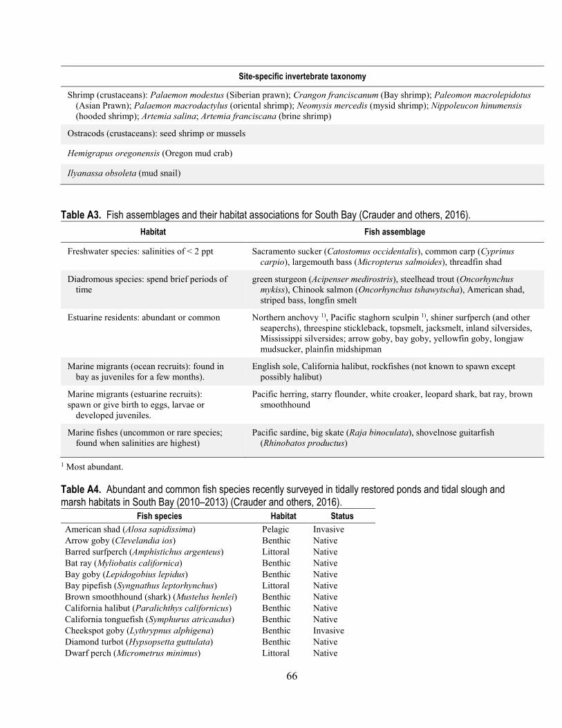
66

Site-specific invertebrate taxonomy

Shrimp (crustaceans): Palaemon modestus (Siberian prawn); Crangon franciscanum (Bay shrimp); Paleomon macrolepidotus (Asian Prawn); Palaemon macrodactylus (oriental shrimp); Neomysis mercedis (mysid shrimp); Nippoleucon hinumensis (hooded shrimp); Artemia salina; Artemia franciscana (brine shrimp)

Ostracods (crustaceans): seed shrimp or mussels Hemigrapus oregonensis (Oregon mud crab) Ilyanassa obsoleta (mud snail)

Table A3. Fish assemblages and their habitat associations for South Bay (Crauder and others, 2016). Habitat Fish assemblage

Freshwater species: salinities of < 2 ppt Sacramento sucker (Catostomus occidentalis), common carp (Cyprinus carpio), largemouth bass (Micropterus salmoides), threadfin shad

Diadromous species: spend brief periods of time

green sturgeon (Acipenser medirostris), steelhead trout (Oncorhynchus mykiss), Chinook salmon (Oncorhynchus tshawytscha), American shad, striped bass, longfin smelt

Estuarine residents: abundant or common Northern anchovy 1), Pacific staghorn sculpin 1), shiner surfperch (and other seaperchs), threespine stickleback, topsmelt, jacksmelt, inland silversides, Mississippi silversides; arrow goby, bay goby, yellowfin goby, longjaw mudsucker, plainfin midshipman

Marine migrants (ocean recruits): found in bay as juveniles for a few months).

English sole, California halibut, rockfishes (not known to spawn except possibly halibut)

Marine migrants (estuarine recruits): spawn or give birth to eggs, larvae or

developed juveniles.

Pacific herring, starry flounder, white croaker, leopard shark, bat ray, brown smoothhound

Marine fishes (uncommon or rare species; found when salinities are highest)

Pacific sardine, big skate (Raja binoculata), shovelnose guitarfish (Rhinobatos productus)

1 Most abundant.

Table A4. Abundant and common fish species recently surveyed in tidally restored ponds and tidal slough and marsh habitats in South Bay (2010–2013) (Crauder and others, 2016).

Fish species Habitat Status American shad (Alosa sapidissima) Pelagic Invasive Arrow goby (Clevelandia ios) Benthic Native Barred surfperch (Amphistichus argenteus) Littoral Native Bat ray (Myliobatis californica) Benthic Native Bay goby (Lepidogobius lepidus) Benthic Native Bay pipefish (Syngnathus leptorhynchus) Littoral Native Brown smoothhound (shark) (Mustelus henlei) Benthic Native California halibut (Paralichthys californicus) Benthic Native California tonguefish (Symphurus atricaudus) Benthic Native Cheekspot goby (Lythrypnus alphigena) Benthic Invasive Diamond turbot (Hypsopsetta guttulata) Benthic Native Dwarf perch (Micrometrus minimus) Littoral Native

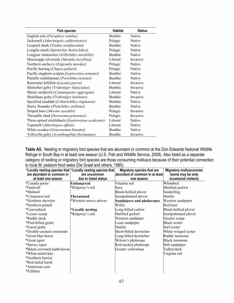
67

Fish species Habitat Status English sole (Parophrys vetulus) Benthic Native Jacksmelt (Atherinopsis californiensis) Pelagic Native Leopard shark (Triakis semifasciata) Benthic Native Longfin smelt (Spirinchus thaleichthys) Pelagic Native Longjaw mudsucker (Gillichthys mirabilis) Benthic Native Mississippi silverside (Menidia beryllina) Littoral Invasive Northern anchovy (Engraulis mordax) Pelagic Native Pacific herring (Clupea pallasii) Pelagic Native Pacific staghorn sculpin (Leptocottus armatus) Benthic Native Plainfin midshipman (Porichthys notatus) Benthic Native Rainwater killifish (Lucania parva) Littoral Invasive Shimofuri goby (Tridentiger bifasciatus) Benthic Invasive Shiner surfperch (Cymatogaster aggregata) Littoral Native Shokihaze goby (Tridentiger barbatus) Benthic Invasive Speckled sanddab (Citharichthys stigmaeus) Benthic Native Starry flounder (Platichthys stellatus) Benthic Native Striped bass (Morone saxatilis) Pelagic Invasive Threadfin shad (Dorosoma petenense) Pelagic Invasive Three-spined stickleback (Gasterosteus aculeatus) Littoral Native Topsmelt (Atherinopos affinis) Littoral Native White croaker (Genyonemus lineatus) Benthic Native Yellowfin goby (Acanthogobius flavimanus) Benthic Invasive

Table A5. Nesting or migratory bird species that are abundant or common at the Don Edwards National Wildlife Refuge in South Bay in at least one season (U.S. Fish and Wildlife Service, 2008). Also listed as a separate category of nesting or migratory bird species are those consuming molluscs because of their potential connection to local M. petalum food webs (De Graaf and others, 1985). *Locally nesting species that are abundant or common in

at least one season *Locally nesting species that

are uncommon due to listed status

Migratory species that are abundant or common in at least

one season

Migratory molluscovores (some may be only occasional visitors)

*Canada goose Endangered Virginia rail Whimbrel *Gadwall *Ridgway’s rail Sora Marbled godwit *Mallard Black-bellied plover Sanderling *Cinnamon teal Threatened Semipalmated plover Dunlin *Northern shoveler *Western snowy plover Sandpipers and phalaropes Western sandpiper *Northern pintail Willet Red knot *Canvasback *Locally nesting

Long-billed curlew Black-bellied plover

*Lesser scaup *Ridgway’s rail Marbled godwit Semipalmated plover *Ruddy duck Western sandpiper Greater scaup *Pied-billed grebe Least sandpiper Black scoter *Eared grebe Dunlin Surf scoter *Double-crested cormorant Short-billed dowitcher White-winged scoter *Great blue heron Long-billed dowitcher Ruddy turnstone *Great egret Wilson’s phalarope Black turnstone *Snowy egret Red-necked phalarope Stilt sandpiper *Black-crowned night-heron Greater yellowlegs Tufted duck *White-tailed kite Virginia rail *Northern harrier *Red-tailed hawk *American coot *Killdeer

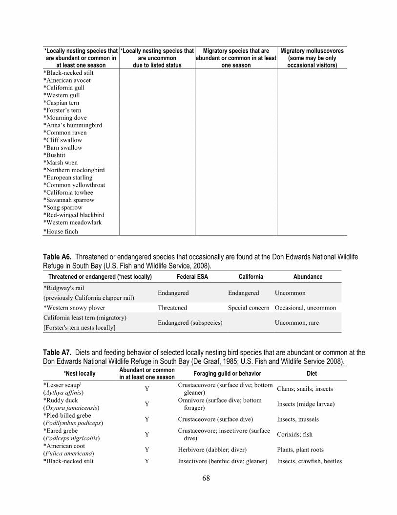
68

*Locally nesting species that are abundant or common in

at least one season *Locally nesting species that

are uncommon due to listed status

Migratory species that are abundant or common in at least

one season

Migratory molluscovores (some may be only occasional visitors)

*Black-necked stilt *American avocet *California gull *Western gull *Caspian tern *Forster’s tern *Mourning dove *Anna’s hummingbird *Common raven *Cliff swallow *Barn swallow *Bushtit *Marsh wren *Northern mockingbird *European starling *Common yellowthroat *California towhee *Savannah sparrow *Song sparrow *Red-winged blackbird *Western meadowlark *House finch

Table A6. Threatened or endangered species that occasionally are found at the Don Edwards National Wildlife Refuge in South Bay (U.S. Fish and Wildlife Service, 2008).

Threatened or endangered (*nest locally) Federal ESA California Abundance *Ridgway's rail

Endangered Endangered Uncommon (previously California clapper rail) *Western snowy plover Threatened Special concern Occasional, uncommon California least tern (migratory)

Endangered (subspecies)

Uncommon, rare [Forster's tern nests locally]

Table A7. Diets and feeding behavior of selected locally nesting bird species that are abundant or common at the Don Edwards National Wildlife Refuge in South Bay (De Graaf, 1985; U.S. Fish and Wildlife Service 2008).

*Nest locally Abundant or common in at least one season Foraging guild or behavior Diet

*Lesser scaup1 (Aythya affinis) Y Crustaceovore (surface dive; bottom

gleaner) Clams; snails; insects

*Ruddy duck (Oxyura jamaicensis) Y Omnivore (surface dive; bottom

forager) Insects (midge larvae)

*Pied-billed grebe (Podilymbus podiceps) Y Crustaceovore (surface dive) Insects, mussels

*Eared grebe (Podiceps nigricollis) Y Crustaceovore; insectivore (surface

dive) Corixids; fish

*American coot (Fulica americana) Y Herbivore (dabbler; diver) Plants, plant roots

*Black-necked stilt Y Insectivore (benthic dive; gleaner) Insects, crawfish, beetles

69

*Nest locally Abundant or common in at least one season Foraging guild or behavior Diet

(Himantopus mexicanus) *American avocet (Recurvirostra americana) Y Omnivore (benthic dive; gleaner) Insects

*Killdeer (Charadrius vociferus) Y Insectivore (shoreline gleaner) Insects

*Forster’s tern (Sterna forsteri) Y Piscivore (water plunger)

insectivore (surface gleaner) Small fish, arthropods

*Double-crested cormorant (Phalacrocorax auritus) Y Piscivore (diving) Fish

1 Scaup and also scoter are of interest to assessments of human health.

Table A8. Diets and feeding behavior of threatened or endangered bird species found at the Don Edwards National Wildlife Refuge in South Bay (De Graaf, 1985; U.S. Fish and Wildlife Service 2008).

Threatened or endangered (*nest locally) Foraging guild or behavior Diet

*Ridgway's rail (previously California clapper rail)

Molluscovore (salt marsh gleaner, shallow probing)

Opportunistic (crabs1, crustaceans1, insects, amphipods, slugs, fish, eggs, plant matter)

*Western snowy plover Crustaceovore (shoreline gleaner)

Juvenile crabs, beetles, flies, worms1; amphipods, clams

California least tern (migratory) (Forster’s tern nests locally) Piscivore (water plunger) Small fish1; small crustaceans, insects

1 Invertebrate considered important to diet.

Table A9. Fish species common in the South Bay that serve as the diet for terns (Ackerman and others, 2014) and known predator fish species that are also benthic feeders.

Species as diet for terns Fish traits relevant to South Bay Mississippi silversides Food-web linkage from sloughs to wider south bay Northern anchovy Topsmelt Pacific staghorn sculpin Three-spined stickleback One-year life span; in loosely aggregated shoals Rainwater killifish Yellowfin goby Longjaw mudsucker Benthic goby species; 2-year life span; small home range; tidal sloughs, mudflats, ponds Prickly sculpin (Cottus asper) Shiner surfperch

Predator species Fish traits relevant to South Bay White sturgeon Benthic feeders White croaker Benthic feeders Leopard shark Benthic feeders

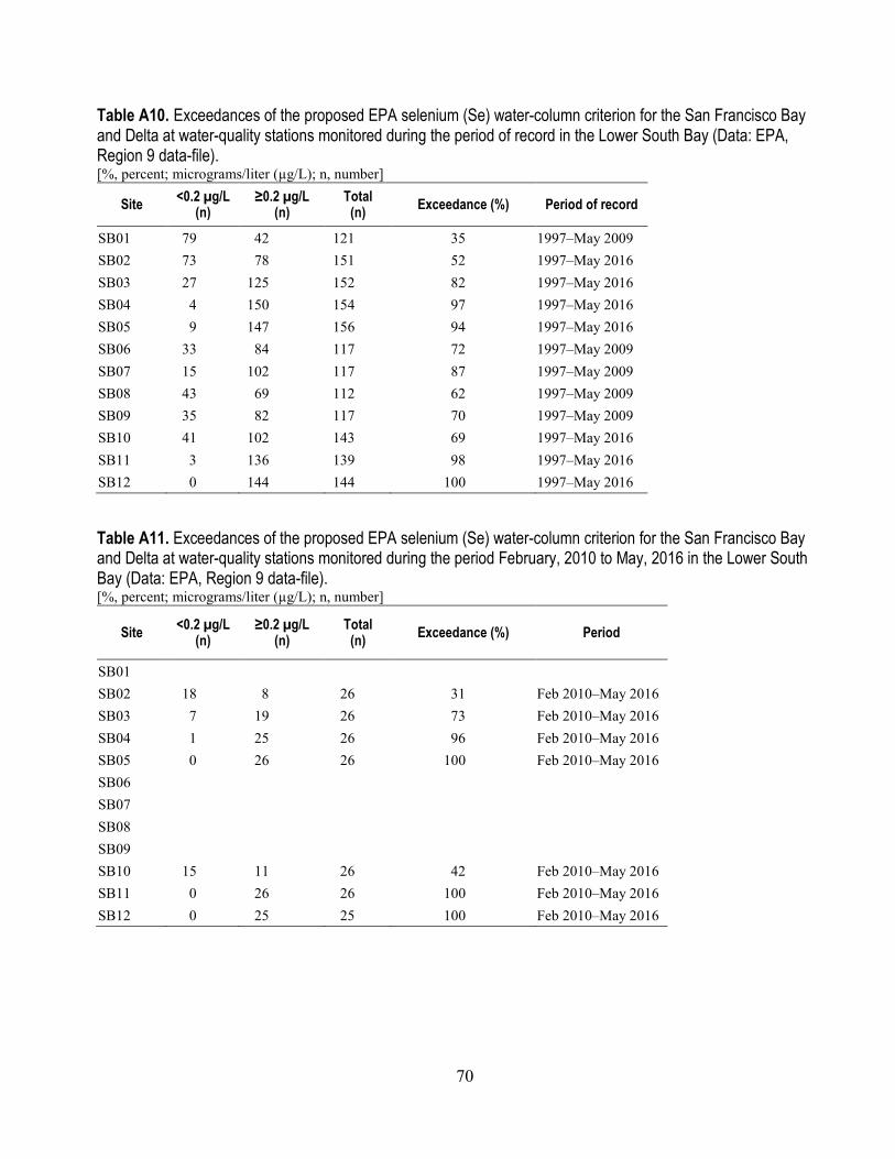
70

Table A10. Exceedances of the proposed EPA selenium (Se) water-column criterion for the San Francisco Bay and Delta at water-quality stations monitored during the period of record in the Lower South Bay (Data: EPA, Region 9 data-file). [%, percent; micrograms/liter (µg/L); n, number]

Site <0.2 µg/L (n)

≥0.2 µg/L (n)

Total (n) Exceedance (%) Period of record

SB01 79 42 121 35 1997–May 2009 SB02 73 78 151 52 1997–May 2016 SB03 27 125 152 82 1997–May 2016 SB04 4 150 154 97 1997–May 2016 SB05 9 147 156 94 1997–May 2016 SB06 33 84 117 72 1997–May 2009 SB07 15 102 117 87 1997–May 2009 SB08 43 69 112 62 1997–May 2009 SB09 35 82 117 70 1997–May 2009 SB10 41 102 143 69 1997–May 2016 SB11 3 136 139 98 1997–May 2016 SB12 0 144 144 100 1997–May 2016

Table A11. Exceedances of the proposed EPA selenium (Se) water-column criterion for the San Francisco Bay and Delta at water-quality stations monitored during the period February, 2010 to May, 2016 in the Lower South Bay (Data: EPA, Region 9 data-file). [%, percent; micrograms/liter (µg/L); n, number]

Site <0.2 µg/L (n)

≥0.2 µg/L (n)

Total (n) Exceedance (%) Period

SB01 SB02 18 8 26 31 Feb 2010–May 2016 SB03 7 19 26 73 Feb 2010–May 2016 SB04 1 25 26 96 Feb 2010–May 2016 SB05 0 26 26 100 Feb 2010–May 2016 SB06 SB07 SB08 SB09 SB10 15 11 26 42 Feb 2010–May 2016 SB11 0 26 26 100 Feb 2010–May 2016 SB12 0 25 25 100 Feb 2010–May 2016

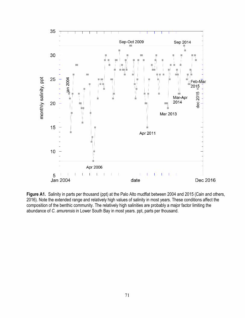
71

Figure A1. Salinity in parts per thousand (ppt) at the Palo Alto mudflat between 2004 and 2015 (Cain and others, 2016). Note the extended range and relatively high values of salinity in most years. These conditions affect the composition of the benthic community. The relatively high salinities are probably a major factor limiting the abundance of C. amurensis in Lower South Bay in most years. ppt, parts per thousand.

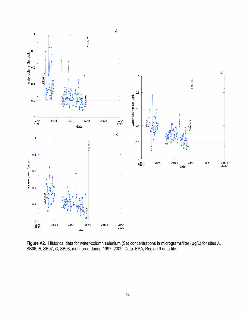
72

Figure A2. Historical data for water-column selenium (Se) concentrations in micrograms/liter (µg/L) for sites A, SB06; B, SB07; C, SB08; monitored during 1997–2009. Data: EPA, Region 9 data-file.

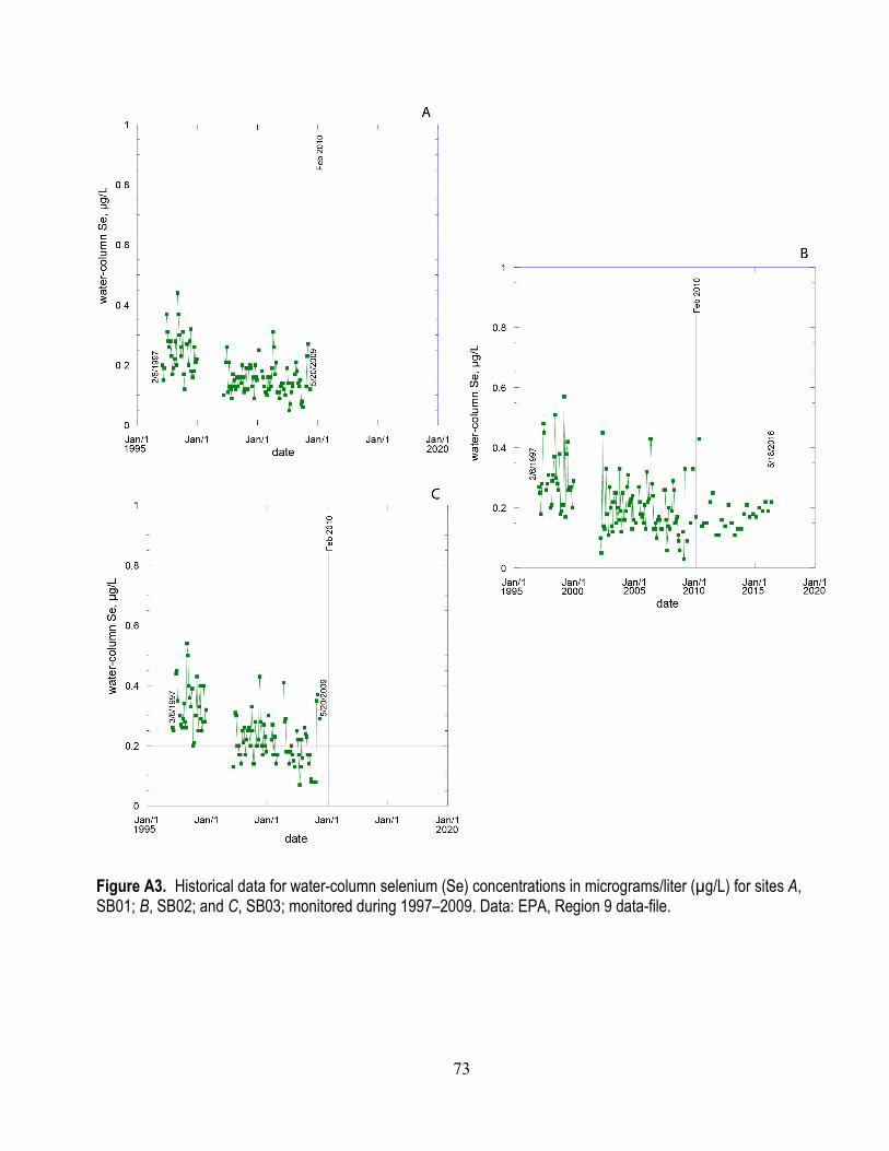
73

Figure A3. Historical data for water-column selenium (Se) concentrations in micrograms/liter (µg/L) for sites A, SB01; B, SB02; and C, SB03; monitored during 1997–2009. Data: EPA, Region 9 data-file.

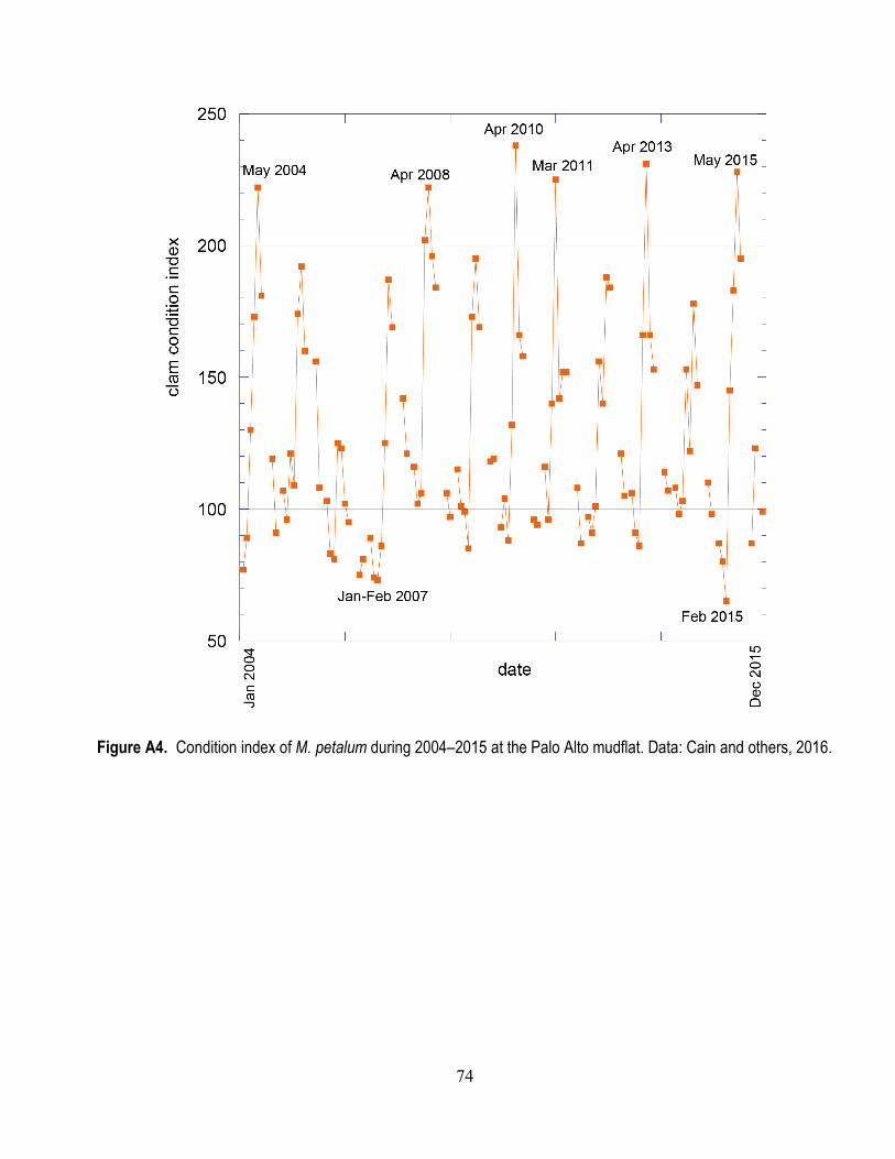
74

Figure A4. Condition index of M. petalum during 2004–2015 at the Palo Alto mudflat. Data: Cain and others, 2016.

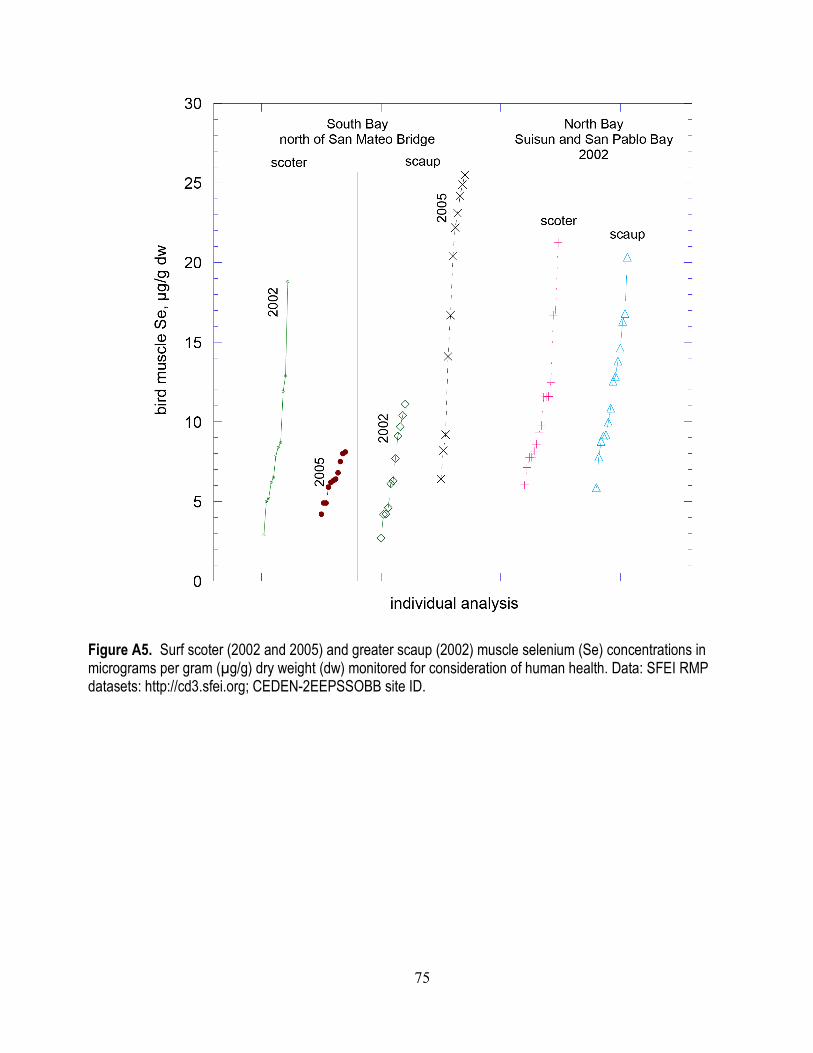
75

Figure A5. Surf scoter (2002 and 2005) and greater scaup (2002) muscle selenium (Se) concentrations in micrograms per gram (µg/g) dry weight (dw) monitored for consideration of human health. Data: SFEI RMP datasets: http://cd3.sfei.org; CEDEN-2EEPSSOBB site ID.

ISSN 2331-1258 (online) https://doi.org/10.3133/ofr20181105

https://doi.org/10.3133/ofr20181105

Luoma and Presser—

Status of Selenium in South San Francisco B

ay—Open-File Report 2018–1105

Documents

Open-File Report 2018-1105: Status of Selenium in South