Embed Size (px)
Citation preview

OPERATION OF CASCADE DAMS
CONSIDERING VARIOUS SCENARIOS
AND FINANCIAL ANALYSIS OF SCENARIOS
A THESIS SUBMITTED TO
THE GRADUATE SCHOOL OF NATURAL AND APPLIED SCIENCES
OF
MIDDLE EAST TECHNICAL UNIVERSITY
BY
BERKER YALIN İMAMOĞLU
IN PARTIAL FULFILLMENT OF THE REQUIREMENTS FOR
THE DEGREE OF MASTER OF SCIENCE
IN
CIVIL ENGINEERING
JANUARY 2013


Approval of the thesis:
OPERATION OF CASCADE DAMS
CONSIDERING VARIOUS SCENARIOS
AND FINANCIAL ANALYSIS OF SCENARIOS
submitted by BERKER YALIN İMAMOĞLU in partial fulfillment of the requirements for the degree of Master of Science in Civil Engineering Department, Middle East Technical University
by,
Prof. Dr. Canan Özgen ____________________
Dean, Graduate School of Natural and Applied Sciences
Prof. Dr. Ahmet Cevdet Yalçıner ____________________
Head of Department, Civil Engineering
Assoc. Prof. Dr. Zuhal Akyürek ____________________
Supervisor, Civil Engineering Dept., METU
Examining Committee Members:
Prof. Dr. A. Melih Yanmaz ____________________
Civil Engineering Dept., METU
Assoc. Prof. Dr. Zuhal Akyürek ____________________
Civil Engineering Dept., METU
Assist. Prof. Dr. Şahnaz Tiğrek ____________________
Civil Engineering Dept., METU
Assoc. Prof. Dr. Nuri Merzi ____________________
Civil Engineering Dept., METU
Ayşe Soydam Baş, M. Sc. Civil Engineer ____________________
Temelsu International Engineering Services Inc.
Date: 15.01.2013

iv
I hereby declare that all information in this document has been obtained and presented in
accordance with academic rules and ethical conduct. I also declare that, as required by these
rules and conduct, I have fully cited and referenced all material and results that are not original
to this work.
Name, Last Name : BERKER YALIN İMAMOĞLU
Signature :

v
ABSTRACT
OPERATION OF CASCADE DAMS
CONSIDERING VARIOUS SCENARIOS
AND FINANCIAL ANALYSIS OF SCENARIOS
İmamoğlu, Berker Yalın
M.Sc., Department of Civil Engineering
Supervisor: Assoc. Prof. Dr. Zuhal Akyürek
January 2013, 158 pages
In assuring the energy supply of Turkey, hydroelectric energy plays one of the most important roles in plans formulated to realize equilibrium between energy production and consumption. Hydroelectric
power plants’ development on Murat River, a tributary of Euphrates, is a part of the development plan
for energy production.
Operation of four dams in cascade on Murat River are simulated by using program package HEC-ResSim. For this purpose, ten scenarios are formulated to utilize the hydraulic potential of Murat
River between the elevations of 870 m – 1225 m. This study provides detailed financial analyses of
scenarios and shows how HEC-ResSim program can be used in formulation of alternative scenarios.
Electric energy storage requirement due to the rising demand for peaking power is creating a completely new market value, which is also increasing the attractiveness of pumped storage power
plants. The results of the simulation performed in Scenario 10 in which two pumped storage power
plants are considered have 15% higher internal rate of return value than the other scenarios with
conventional turbines. Results demonstrate the increasing attractiveness of the cascade system with reversible pump turbines.
Keywords: HEC-ResSim, Reservoir Operation, Simulation, Pumped Storage Hydropower Plants

vi
ÖZ
ARDIŞIK BARAJLARIN ÇESİTLİ SENARYOLAR
DÜŞÜNÜLEREK İŞLETİLMESİ VE
SENARYOLARIN FİNANSAL ANALİZİ
İmamoğlu, Berker Yalın
Yüksek Lisans, İnşaat Mühendisliği Bölümü
Tez Yöneticisi: Doç. Dr. Zuhal Akyürek
Ocak 2013, 158 sayfa
Hidroelektrik enerji; arz ve talep arasındaki dengeyi sağlamak için yapılan planlamalarda, Türkiye’nin
enerji arzını güvence altına alarak en önemli rollerden birini oynar. Fırat Nehri’nin bir kolu olan
Murat Nehri üzerindeki hidroelektrik santraller enerji üretimi için yapılan kalkınma planlamasının bir parçasıdır.
Murat Nehri üzerindeki ardışık dört barajın işletilmesi HEC-ResSim paket programı kullanılarak benzeşimleri sağlanmıştır. Bu amaçla, Murat Nehri’nin 870 m - 1225 m kotları arasındaki hidrolik
potansiyelini kullanmak için on senaryo tasarlanmıştır. Bu çalışma senaryoların detaylı bir finansal
analizini sunmakta ve HEC-ResSim programının alternatif senaryoların formülasyonunda
kullanılabileceği anlatmaktadır.
Pik güç talebinde olan artış nedeniyle doğan elektrik enerjisi depolama ihtiyacı tamamen yeni bir
piyasa değeri yaratarak, pompaj depolamalı santrallerin çekiciliğini arttırmaktadır. İki pompaj
depolamalı santralin modellendiği Senaryo 10’nun diğer depolamalı santralli senaryolara kıyasla %15
daha fazla bir iç karlılık oranına sahip olduğu görülmüştür. Sonuçlar pompa türbinlerine sahip ardışık
sistemin cazibesinin arttığını göstermektedir.
Anahtar Kelimeler: HEC-ResSim, Baraj İşletmesi, Benzeşim, Pompaj Depolamalı Hidroelektrik
Santraller

vii
To My Parents...

viii
ACKNOWLEDGEMENTS
I would like to state that I am grateful to my advisor Doç. Dr. Zuhal AKYÜREK for her
contributions, support from the initial to final level, who influenced and reshaped my career, future plans and expectations by her perfectionism, motivation of achievement and positive reinforcements.
I am also grateful to my dear wife, Esen İMAMOĞLU for her encouragement, positive motivation
and endless support in hard times.
I owe my deepest graditute to my dear mom, Canan İMAMOĞLU and to my dear dad, Cemal
İMAMOĞLU for their patience, endless support, interest and encouragement.
The assistance of the Temelsu Inc. staff is gratefully acknowledged. In addition to the information
furnished, the employees officials of Temelsu were particularly helpful in suggesting and arranging
meetings and in providing advice and background information.
Finally, I would like to thank to my friend and manager, Ayse SOYDAM BAŞ for all her best wishes.
This study could not be completed without you. I am so grateful to you.

ix
TABLE OF CONTENTS
ABSTRACT ................................................................................................................................... v
ÖZ.... ............................................................................................................................................. vi
ACKNOWLEDGEMENTS ........................................................................................................viii
TABLE OF CONTENTS .............................................................................................................. ix
LIST OF FIGURES ...................................................................................................................... xi
LIST OF TABLES ...................................................................................................................... xiv
CHAPTERS
1. INTRODUCTION ................................................................................................................. 1
2. LITERATURE REVIEW ..................................................................................................... 5
2.1 Water Power Equation .................................................................................................. 5 2.2 Storage Zones .............................................................................................................. 6
2.3 Hydropower Potential of Turkey ................................................................................... 6
2.4 Pumped Storage ......................................................................................................... 14
2.5 Mathematical Formulation of the Model ..................................................................... 18
2.5.1 Storage Volume Constraint .................................................................................... 18
2.5.2 Release Constraint ................................................................................................. 18
2.5.3 State Transformation Equation ............................................................................... 19
2.6 Reservoir Simulation Models ...................................................................................... 19
2.6.1 HEC-5 ................................................................................................................... 19
2.6.2 WEAP ................................................................................................................... 19
2.6.3 MIKE BASIN ........................................................................................................ 20
2.6.4 HEC-ResSim ......................................................................................................... 21
3. KALEKÖY CASCADE RESERVOIR SYSTEM ............................................................... 23
3.1 Description of Watershed ............................................................................................... 23
3.2 Installed Capacity........................................................................................................... 27
3.3 Hydrology...................................................................................................................... 29
3.3.1 Climate .................................................................................................................. 29
3.3.2 Reservoir Inflows .................................................................................................. 30
3.3.3 Environmental Flows ............................................................................................. 36
3.3.4 Trends in River Flow ............................................................................................. 36
3.3.5 Evaporation ........................................................................................................... 37 3.3.6 Sediment Yield ...................................................................................................... 38
3.4 Reservoir Storage ........................................................................................................... 39
3.5 Tailwater Rating Curves ................................................................................................. 41
3.6 Head Losses ................................................................................................................... 44
3.7 Efficiency ...................................................................................................................... 44
3.8 Dams’ Features .............................................................................................................. 44
3.8.1 Upper Kaleköy Dam and HEPP ............................................................................. 44
3.8.2 Lower Kaleköy Dam and HEPP ............................................................................. 44
3.8.3 Beyhan 1 Dam and HEPP ...................................................................................... 45
3.8.4 Beyhan 2 Dam and HEPP ...................................................................................... 45
3.7 Models Components in HEC-ResSim ............................................................................. 46
3.8 Model Set-up in HEC-ResSim ........................................................................................ 47
4. SIMULATION ANALYSIS ................................................................................................ 55
4.1 Introduction ................................................................................................................... 55
4.2 Scenario 1 ...................................................................................................................... 60
4.3 Scenario 2 ...................................................................................................................... 64
4.4 Scenario 3 ...................................................................................................................... 66
4.5 Scenario 4 ...................................................................................................................... 77

x
4.6 Scenario 5 ...................................................................................................................... 77
4.7 Scenario 6 ...................................................................................................................... 79
4.8 Scenario 7 ...................................................................................................................... 83
4.9 Pumped Storage Scenarios ............................................................................................. 87
4.9.1 Scenario 8 .............................................................................................................. 90
4.9.2 Scenario 9 .............................................................................................................. 94
4.9.3 Scenario 10 ............................................................................................................ 94
5. FINANCIAL ANALYSIS .................................................................................................... 97
5.1 Introduction ................................................................................................................... 97 5.2 Cost of Facilities ............................................................................................................ 97
5.3 Direct and Investment Costs ........................................................................................... 98
5.3.1 Direct Costs ........................................................................................................... 98
5.3.2 Project Costs .......................................................................................................... 98
5.3.3 Investment Program and Investment Cost ............................................................... 98
5.4 Annual Costs.................................................................................................................. 99
5.5 Annual Benefits ........................................................................................................... 108
5.6 Benefit – Cost Analyses ............................................................................................... 114
5.7 Internal Rate of Return ................................................................................................. 117
6. DISCUSSION OF RESULTS ............................................................................................ 119
6.1 Discussion of Results ................................................................................................... 119
7. CONCLUSION AND RECOMMENDATIONS ............................................................... 123
7.1 Conclusion ................................................................................................................... 123
7.2 Recommendations ........................................................................................................ 123
BIBLIOGRAPHY ...................................................................................................................... 125
APPENDICES
A. INTERNAL RATE OF RETURN CALCULATIONS ..................................................... 127
B. THE CHARACTERISTICS OF RESERVOIRS .............................................................. 147

xi
LIST OF FIGURES
FIGURES
Figure 2.1 Storage Zones ................................................................................................................... 6
Figure 2.2 Energy generation of European countries, 2009 (Investment Support and Promotion
Agency, 2010) ........................................................................................................................ 7 Figure 2.3 Development of Turkey’s electric generation and distribution of sources (Saraç, 2012) ...... 8
Figure 2.4 Hydropower potential of Turkey (General Directorate of Renewable Energy, 2012) ........... 8
Figure 2.5 Number of dams under operation in Turkey’s basins (Alantor et al., 2012) ......................... 9
Figure 2.6 Turkey’s installed capacity ratios according to sources – September 2012 (İnci, 2012) ..... 10
Figure 2.7 Development of the peak demand by years (Energy Market Regulatory Authority, 2011) . 11
Figure 2.8 Development of reserve margins according to installed capacities (Energy Market
Regulatory Authority, 2012) .................................................................................................. 13
Figure 2.9 Reserve margins according to total and firm energy generation capacities (Energy Market
Regulatory Authority, 2012) .................................................................................................. 13
Figure 2.10 World Pumped Storage Potential (Saraç, 2012) .............................................................. 14
Figure 2.11 Types of pumped turbines (Voith, 2009) ........................................................................ 16
Figure 2.12 Types of pumped storages development (Voith, 2009) ................................................... 17 Figure 2.13 WEAP Network View (Rukuni, 2006) ........................................................................... 20
Figure 2.14 MIKE BASIN Network View (University of Texas, 2012) ............................................. 21
Figure 3.1 Location of the Kaleköy reservoir system on map of Turkey (World Map, 2012) .............. 24
Figure 3.2 Hydropower plants’ layout in the basin (Temelsu International Engineering Services Inc.,
2011) .................................................................................................................................... 25
Figure 3.3 Schematic diagram of Kaleköy reservoir system .............................................................. 26
Figure 3.4 Profile of Kaleköy reservoir system ................................................................................. 28
Figure 3.5 Annual inflow of Upper Kaleköy reservoir in existing case .............................................. 31
Figure 3.6 Annual flow duration curve of Upper Kaleköy reservoir in existing case .......................... 31
Figure 3.7 Annual inflow of Upper Kaleköy reservoir in full development case ................................ 32
Figure 3.8 Annual flow duration curve of Upper Kaleköy reservoir in full development case ............ 32 Figure 3.9 Annual intermediate inflow between Upper Kaleköy reservoir and Lower Kaleköy
reservoir in existing and full development case ...................................................................... 33
Figure 3.10 Annual flow duration curve of intermediate inflow between Upper Kaleköy and Lower
Kaleköy reservoir in existing and full development case ........................................................ 33
Figure 3.11 Annual intermediate inflow between Lower Kaleköy reservoir and Beyhan 1 reservoir in
existing and full development case ........................................................................................ 34
Figure 3.12 Annual flow duration curve of intermediate inflow between Lower Kaleköy reservoir and
Beyhan 1 reservoir in existing and full development case ....................................................... 34
Figure 3.13 Comparison of monthly inflow at Upper Kaleköy reservoir in existing and full
development case .................................................................................................................. 35
Figure 3.14 Monthly evaporation data for Upper and Lower Kaleköy Dams and HEPPs ................... 37
Figure 3.15 Monthly evaporation data for Beyhan 1 and Beyhan 2 Dams and HEPPs ........................ 37 Figure 3.16 Recommended submergence for intakes (ASCE, 1995) .................................................. 39
Figure 3.17 Elevation-area curve for Upper Kaleköy Dam ................................................................ 39
Figure 3.18 Elevation-area curve for Lower Kaleköy Dam................................................................ 40
Figure 3.19 Elevation-area curve for Beyhan 1 Dam ......................................................................... 40
Figure 3.20 Elevation-area curve for Beyhan 2 Dam ......................................................................... 41
Figure 3.21 Tailwater rating curve for the dam site of Upper Kaleköy ............................................... 42
Figure 3.22 Tailwater rating curve for the dam site of Lower Kaleköy .............................................. 42
Figure 3.23 Tailwater rating curve for the dam site of Beyhan 1........................................................ 43
Figure 3.24 Tailwater rating curve for the dam site of Beyhan 2........................................................ 43
Figure 3.25 HEC-ResSim Module concepts (Klipsch, 2007) ............................................................. 46
Figure 3.26 Reservoir Network Module, Kaleköy cascade reservoir system ...................................... 48 Figure 3.27 Reservoir editor tab, physical properties of hydraulic structures...................................... 48
Figure 3.28 Reservoir Editor, operating rules.................................................................................... 49

xii
Figure 3.29 Specification of release allocation strategy with the HEC-ResSim Reservoir Editor ........ 50
Figure 3.30 Pump Rule Editor .......................................................................................................... 51
Figure 3.31 Graphical display of "Default plot" function ................................................................... 52
Figure 3.32 Graphical display of "Power plot" function .................................................................... 53
Figure 3.33 Graphical display of "Releases plot" function ................................................................. 54
Figure 4.1 Upper Kaleköy reservoir storage required vs. height for 600 MW plant with 6, 12, 18 and
24 hours of operation ............................................................................................................ 56
Figure 4.2 Lower Kaleköy reservoir storage required vs. height for 450 MW plant with 6, 12, 18 and
24 hours of operation ............................................................................................................ 57
Figure 4.3 Beyhan 1 reservoir storage required vs. height for 550 MW plant with 6, 12, 18 and 24
hours of operation ................................................................................................................. 57 Figure 4.4 Beyhan 2 reservoir storage required vs. height for 255 MW plant with 6, 12, 18 and 24
hours of operation ................................................................................................................. 58
Figure 4.5 Seasonal variation editor.................................................................................................. 59
Figure 4.6 Seasonal variation editor graph for Lower Kaleköy .......................................................... 59
Figure 4.7 A part of daily operating cycle for Upper Kaleköy reservoir storage ................................. 61
Figure 4.8 A Power and net-inflow duration curve at Upper Kaleköy reservoir in Scenario 1 ............ 62
Figure 4.9 A Power and net-inflow duration curve at Lower Kaleköy reservoir in Scenario 1 ........... 63
Figure 4.10 A Power and net-inflow duration curve at Beyhan 1 reservoir in Scenario 1 ................... 63
Figure 4.11 A Power and net-inflow duration curve at Beyhan 2 reservoir in Scenario 1 ................... 64
Figure 4.12 %10 percent increase in local inflow at computation point .............................................. 65
Figure 4.13 Application of firm power generation requirement rule .................................................. 66 Figure 4.14 Allowable turbined release range of Upper Kaleköy in Scenario 3 .................................. 67
Figure 4.15 40 years time series simulation period operating cycle for Upper Kaleköy Dam and HEPP
in Scenario 3 ......................................................................................................................... 69
Figure 4.16 Critical period and critical drawdown period for Upper Kaleköy Dam and HEPP in
Scenario 3 ............................................................................................................................. 70
Figure 4.17 40 years time series simulation period operating cycle for Lower Kaleköy Dam and HEPP
in Scenario 3 ......................................................................................................................... 71
Figure 4.18 40 years time series simulation period operating cycle for Beyhan 1 Dam and HEPP in
Scenario 3 ............................................................................................................................. 72
Figure 4.19 40 years time series simulation period operating cycle for Beyhan 2 Dam and HEPP in
Scenario 3 ............................................................................................................................. 73
Figure 4.20 A Power and net-inflow duration curve at Upper Kaleköy reservoir in Scenario 3 ........... 75 Figure 4.21 Power and net-inflow duration curve at Lower Kaleköy reservoir in Scenario 3 .............. 75
Figure 4.22 Power and net-inflow duration curve at Beyhan 1 reservoir in Scenario 3 ....................... 76
Figure 4.23 Power and net-inflow duration curve at Beyhan 2 reservoir in Scenario 3 ....................... 76
Figure 4.24 Revised storage zone at Lower Kaleköy reservoir in Scenario 5...................................... 78
Figure 4.25 A general example of guide curve for Kaleköy reservoir system ..................................... 79
Figure 4.26 Operation guide curves for Kaleköy reservoir system ..................................................... 80
Figure 4.27 40 years time series simulation period operating cycle for Lower Kaleköy Dam and HEPP
in Scenario 6 ......................................................................................................................... 81
Figure 4.28 A closer look to the power plot for the critical period operating cycle for Lower Kaleköy
Dam and HEPP in Scenario 6 ................................................................................................ 82
Figure 4.29 Peak power generation operation cycle for Lower Kaleköy Dam and HEPP in Scenario 7 ............................................................................................................................. 84
Figure 4.30 Power and net-inflow duration curve at Upper Kaleköy reservoir in Scenario 7 .............. 85
Figure 4.31 Power and net-inflow duration curve at Lower Kaleköy reservoir in Scenario 7 .............. 86
Figure 4.32 Power and net-inflow duration curve at Beyhan 1 reservoir in Scenario 7 ....................... 86
Figure 4.33 Power and net-inflow duration curve at Beyhan 2 reservoir in Scenario 7 ....................... 87
Figure 4.34 Reservoir editor tab to define the physical characteristics of pump.................................. 88
Figure 4.35 Hour of day multiplier with values of 0.0 and 1.0 specified for a portion of day .............. 89
Figure 4.36 Performance range for pump-turbines (Voith, 2009) ....................................................... 90
Figure 4.37 Visual presentation of Scenario 8 ................................................................................... 91
Figure 4.38 40 years long time series simulation period operating cycle for Upper Kaleköy Dam and
HEPP in Scenario 8 ............................................................................................................... 91
Figure 4.39 Peak operation of Scenario 9.......................................................................................... 93 Figure 4.40 Visual presentation of Scenario 9 ................................................................................... 95
Figure 5.1 General structure of the financial model ........................................................................... 97

xiii
Figure 6.1 Location Internal rate of return values (%) for Scenarios ................................................. 119
Figure 6.2 Annual Total Energy Generation (GWh/year) for Scenarios ............................................ 120
Figure 6.3 Annual Energy Benefit (TL/year) for Scenarios .............................................................. 121
Figure 6.4 Benefit/Cost Ratios for Scenarios ................................................................................... 122
Figure A.1 Cash flow graph for Scenario 1 ...................................................................................... 128
Figure A.2 Cash flow graph for Scenario 2 ...................................................................................... 130
Figure A.3 Cash flow graph for Scenario 3 ...................................................................................... 132
Figure A.4 Cash flow graph for Scenario 4 ...................................................................................... 134
Figure A.5 Cash flow graph for Scenario 5 ...................................................................................... 136
Figure A.6 Cash flow graph for Scenario 6 ...................................................................................... 138
Figure A.7 Cash flow graph for Scenario 7 ...................................................................................... 140 Figure A.8 Cash flow graph for Scenario 8 ...................................................................................... 142
Figure A.9 Cash flow graph for Scenario 9 ...................................................................................... 144
Figure A.10 Cash flow graph for Scenario 10 .................................................................................. 146
Figure B.1 General plan of Upper Kaleköy Dam and HEPP ............................................................. 148
Figure B.2 Typical cross section of Upper Kaleköy Dam and HEPP ................................................ 149
Figure B.3 General plan of Lower Kaleköy Dam and HEPP ........................................................... 151
Figure B.4 Typical cross section of Lower Kaleköy Dam and HEPP ................................................ 152
Figure B.5 General plan of Beyhan 1 Dam and HEPP ...................................................................... 154
Figure B.6 Typical cross section of Beyhan 1 Dam and HEPP ......................................................... 155
Figure B.7 General plan of Beyhan 2 Dam and HEPP ...................................................................... 157
Figure B.8 Typical cross section of Beyhan 2 Dam and HEPP ......................................................... 158

xiv
LIST OF TABLES
TABLES
Table 2.1 General energy production and consumption of Turkey (Energy Market Regulatory
Authority, 2012)...................................................................................................................... 7
Table 2.2 Installed power capacity of Turkey – September 2012 (İnci, 2012) ...................................... 9
Table 2.3 Estimated peak demand and energy demand according to the high and low scenarios
(Energy Market Regulatory Authority, 2012) ......................................................................... 12
Table 2.4 Development of the installed capacity and energy production for High and Low Demand
Scenarios (Energy Market Regulatory Authority, 2012) ......................................................... 12
Table 2.5 Sources of energy utilization (Lempérière, 2011) .............................................................. 15 Table 3.1 Annual Precipitation and Temperature (Temelsu International Engineering Services Inc.,
2011) .................................................................................................................................... 30
Table 3.2 Environmental Flows ........................................................................................................ 36
Table 3.3 Sediment volumes of reservoirs ........................................................................................ 38
Table 4.1 Storage capacities for the Upper Kaleköy, Lower Kaleköy, Beyhan 1 and Beyhan 2
reservoirs .............................................................................................................................. 56
Table 4.2 Summary of results for Scenario 1 .................................................................................... 62
Table 4.3 Summary of results for Scenario 2 .................................................................................... 64
Table 4.4 Summary of results for Scenario 3 .................................................................................... 74
Table 4.5 Summary of results for Scenario 4 .................................................................................... 77
Table 4.6 Summary of results for Scenario 5 .................................................................................... 78 Table 4.7 Summary of results for Scenario 6 .................................................................................... 80
Table 4.8 Wise-hour schedule .......................................................................................................... 83
Table 4.9 Summary of results for Scenario 7 .................................................................................... 85
Table 4.10 Calculation methodology of consumed pump energy ....................................................... 92
Table 4.11 Summary of results for Scenario 8................................................................................... 92
Table 4.12 Summary of results for Scenario 9................................................................................... 94
Table 4.13 Summary of results for Scenario 10 ................................................................................. 94
Table 5.1 Yearly distribution of investment for Kaleköy reservoir system ......................................... 98
Table 5.2 Renewal and operation-maintenance factors ...................................................................... 99
Table 5.3 Construction costs for Scenario 1, 2, 3, 4, 5, 6 and 7 .........................................................100
Table 5.4 Calculation of investment costs for Scenario 1, 2, 3, 4, 5, 6 and 7 .....................................101
Table 5.5 Calculation of annual costs for Scenario 1, 2, 3, 4, 5, 6 and 7 ............................................101 Table 5.6 Construction costs for Scenario 8 .....................................................................................102
Table 5.7 Calculation of investment costs for Scenario 8 .................................................................103
Table 5.8 Calculation of annual costs for Scenario 8 ........................................................................103
Table 5.9 Construction costs for Scenario 9 .....................................................................................104
Table 5.10 Calculation of investment costs for Scenario 9................................................................105
Table 5.11 Calculation of annual costs for Scenario 9 ......................................................................105
Table 5.12 Construction costs for Scenario 10 .................................................................................106
Table 5.13 Calculation of investment costs for Scenario 10 ..............................................................107
Table 5.14 Calculation of annual costs for Scenario 10 ....................................................................107
Table 5.15 Unit energy benefits .......................................................................................................108
Table 5.16 Calculation of annual benefits for Scenario 1 ..................................................................109 Table 5.17 Calculation of annual benefits for Scenario 2 ..................................................................109
Table 5.18 Calculation of annual benefits for Scenario 3 ..................................................................110
Table 5.19 Calculation of annual benefits for Scenario 4 ..................................................................110
Table 5.20 Calculation of annual benefits for Scenario 5 ..................................................................111
Table 5.21 Calculation of annual benefits for Scenario 6 ..................................................................111
Table 5.22 Calculation of annual benefits for Scenario 7 ..................................................................112
Table 5.23 Calculation of annual benefits for Scenario 8 ..................................................................112
Table 5.24 Calculation of annual benefits for Scenario 9 ..................................................................113
Table 5.25 Calculation of annual benefits for Scenario 10 ................................................................113
Table 5.26 Internal rate of return values for Scenarios .....................................................................117

xv
Table A.1 Internal rate of return for Scenario 1 ................................................................................ 127
Table A.2 Internal rate of return for Scenario 2 ................................................................................ 129
Table A.3 Internal rate of return for Scenario 3 ................................................................................ 131
Table A.4 Internal rate of return for Scenario 4 ................................................................................ 133
Table A.5 Internal rate of return for Scenario 5 ................................................................................ 135
Table A.6 Internal rate of return for Scenario 6 ................................................................................ 137
Table A.7 Internal rate of return for Scenario 7 ................................................................................ 139
Table A.8 Internal rate of return for Scenario 8 ................................................................................ 141
Table A.9 Internal rate of return for Scenario 9 ................................................................................ 143
Table A.10 Internal rate of return for Scenario 10 ............................................................................ 145
Table B.1 The characteristics of Upper Kaleköy Dam ...................................................................... 147 Table B.2 The characteristics of Lower Kaleköy Dam ..................................................................... 150
Table B.3 The characteristics of Beyhan 1 Dam .............................................................................. 153
Table B.4 The characteristics of Beyhan 2 Dam .............................................................................. 156


1
CHAPTER 1
INTRODUCTION
Water and energy are two main resources which are required for humankind and are tightly
connected. As water flows from highlands to a lower elevation, its potential energy is reduced by drop
in elevation, and other causes. A part of this potential energy may be converted to mechanical energy
and used to generate hydropower.
During the nineteenth century, hydropower became a source of electrical energy. In the 1900s, the
generation of electricity expanded the need for larger hydroelectric plants because the transmission of
power over long distances became economical by the installation of alternating current equipments
(Gulliver and Arndt, 1991).
The first benefit of the hydropower is that no air or water pollutants are produced. Since fuel is not
burned, there is minimum pollution. Hydropower also reduces greenhouse gas emissions. Relatively
low operation and maintenance costs are other advantages of hydropower (International Energy
Agency, 2012).
In assuring the energy supply of Turkey, all industrialized and developing nations adopt the principle
that a suitable mix of different energy resources must be relied upon in meeting the energy
consumption with acceptable economy and supply security. It is well-known that hydroelectric power plays one of the most important roles in plans formulated to realize an equilibrium between energy
production and consumption. Alternatives to hydroelectric power generation include nuclear power
plants, thermal power plants, and relatively new technologies relying on geothermal, wind and solar
energy. Import of electric power, which has been practised in the past, could also meet the domestic
electricity demand.
The feasible hydroelectric energy potential of Turkey is estimated to be about 140 GWh/year and as
of year 2011, only 38% of this is generated recently, as the other portion is lost because of incomplete
development of dams and their hydropower plants (Energy Market Regulatory Authority, 2012). However there is a speedy pace of on-going construction of hydropower plants all over Turkey
including many run-of-river types.
Demand forecast is the essence of decision making processes in market activities. Demand for
electricity is basically affected by economic growth, increase in population and urbanization as well
as energy efficiency applications and factors related to climate change (Deloitte Financial Advisory
Services LLP, 2010).
Turkey will likely see the fastest medium to long-term growth in energy demand among the
International Energy Agency member countries. Turkey has a young and urbanising population and
energy use is still comparatively low. Therefore, ensuring sufficient energy supply to a growing
economy remains the goverment’s main energy policy concern (International Energy Agency, 2012).
Although Turkish electricity demand forecast should be based on the cumulative demand forecast of each regional distribution company by virtue of the Electricity Market Grid Regulation and
Regulation Concerning Electricity Demand Forecast, currently it is still calculated by Ministry of
Energy and Natural Resources by using Model for Analysis of Energy Demand (MAED). According
to the latest “Turkish Electrical Energy 10-Year Generation Capacity Projection 2011-2020 Report”
published by Turkish Electricity Transmission Company, total electricity demand is expected to reach
398 TWh with 6.7% compound annual growth rate in base scenario and 434 TWh with 7.5% in high
scenario in 2020 (Turkish Electricity Transmission Company, 2011).

2
Directive 2001/77/EC concerning Encouragement of Electricity Production from Renewable Energy
Resources in the Internal Market of Electricity aims at producing 22.1% of the electricity consumed
by the Europian Union member countries from the renewable energy resources (Energy Market
Regulatory Authority, 2011). This provision will require European Union countries to import energy
from abroad. It will be possible to export part of the hydroelectric energy to be produced in Turkey at
convenient prices. However, energy to be produced at thermal or nuclear power plants can also be
imported at cheaper prices. For this reason, surplus supply has to be aimed in the production of green energy in our country.
Accordingly, development of all hydroelectric capacity in the shortest period of time is required
regarding national interest.
With the recent liberalization, the appearance of Turkish electricity energy sector has been changing significantly, the level of competition increasing and more and more players have been entering into
the market every day. 4628 numbered Electricity Market Law and the following Electricity Market
License Regulation have paved way to private entrepreneurs for electricity generation, and granted
them in establishing the power and operating hydroelectric power plants.
Cascade reservoir systems may be complex. Because of the complexity, computer based simulation
programs can be used to provide and perform different scenarios easily. One can use computer based
simulation programs extensively to solve problems with operation rules or operation limitations.
Simulation is a modelling technique that is used to predict the behaviour of the system under a given set of conditions, representing all the characteristics of the system largely by a mathematical or
algebraic description.
HEC-ResSim is a general-purpose reservoir simulation model developed by the Hydrologic
Engineering Center to evaluate a wide variety of flood control and conservation storage projects,
including hydropower analysis. The program can be used efficiently for single reservoirs or for
complete reservoir systems on either critical period or period of record studies.
Upper Fırat Valley of Turkey is the least developed area in terms of the potential value of its water
and land resources. Development of the region over a period of two to three decades would make a
major contribution to Turkey's energy supplies. On the other hand, without development of the region
it is doubtful whether any of these future requirements can be achieved.
The study conducted by Pöyry and Temelsu International Engineering Services Inc., was presented as a feasibility report for water resources management in the Lower Murat basin between 870 m – 1225
m. The feasibility report was carried out in 2011. Maximization of firm energy and operation of
reservoirs in peak mode was studied in the feasibility study. The main goal of this thesis is to improve
the feasibility report by considering different operation scenarios and pumped storage alternatives. In
addition to this, financial analysis has been carried out considering the revenues, the operation and
maintenance costs as well as the capital expenditures.
The objective of this study is
i) to estimate the hydropower potential of the Murat river between 870 m – 1225 m. Various
operation rules and ten different scenarios are performed to investigate the energy generation
potential,
ii) to provide information for long-term planning on the capacity of Kaleköy reservoir system
and respective reservoirs, Upper Kaleköy, Lower Kaleköy, Beyhan 1 and Beyhan 2,
iii) to reduce spillway losses, such that a higher fraction of runoff is used for energy generation,
iv) to maintain high heads and preferentially produce energy when prices are high. This is also
achieved by using the operation guide curves and operation rules,
v) to investigate if the pumped storage applications on the system is feasible or not,
vi) to get information for future investments. Financial analyses are presented for the
comparison of the scenarios.

3
In order to fullfill these objectives, this thesis has seven main chapters including this chapter.
Chapter 2 contains a general information about mathematical formulation of the model, a literature
review section and a brief information about reservoir simulation models.
Characteristics of Kaleköy reservoir system and Lower Murat basin are summarized in Chapter 3.
The results of ten scenarios have been presented to utilize the hydraulic potential of the Murat River
between the elevations of 870 m – 1225 m in Chapter 4.
According to the results of each scenario, the financial anaylses of the scenarios are described in
Chapter 5.
Finally discussion of results and conclusion of the thesis is given in Chapter 6 and Chapter 7,
respectively.

4

5
CHAPTER 2
1. LITERATURE REVIEW
2.1 Water Power Equation
The amount of power that a hydraulic turbine can develop is a function of the quantity of water
available, the net hydraulic head across the turbine, and efficiency of the turbine (Doland, 1954).
The power output of a hydroelectric plant is given by the equation (Yanmaz, 2006):
where
P = generator output in kW
e = overall plant efficiency (a fraction)
= specific weight of water in (kN/m³)
Q = flow through the turbine (m³/s)
H = net head on the turbine (m).
Following is a brief description of the sources of the parameters that make up the power equation. The
source of the flow for hydroelectric plants is snowmelt and rainfall. Since rainfall is quite variable in
quantity and occurence, the resulting runoff is by no means constant. Figure 2.1 shows the gross head
as the difference between the reservoir and tailwater (elevation plus velocity head and head loss) for
any given discharge. The net head on the turbine is the difference between the energy grade line
elevations at the entrance to the turbine case and at tailwater. The efficiency term is the combined
efficiencies of the turbine, transformer and generator.
(2.1) ...)( HQekWP
6
DeadStorageZone
Conservation Zone
Top Inactive
Top Flood Control
Flood Control Zone
Minimum Operation Water Level
Maximum Operation Water Level / Top Conservation
Dam
Body Tailwater Elevation
Head Losses
Net HeadGross Head
HEPP
Figure 2.1 Storage zones
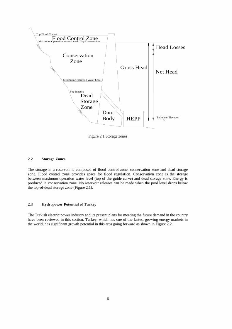
2.2 Storage Zones
The storage in a reservoir is composed of flood control zone, conservation zone and dead storage
zone. Flood control zone provides space for flood regulation. Conservation zone is the storage between maximum operation water level (top of the guide curve) and dead storage zone. Energy is
produced in conservation zone. No reservoir releases can be made when the pool level drops below
the top-of-dead storage zone (Figure 2.1).
2.3 Hydropower Potential of Turkey
The Turkish electric power industry and its present plans for meeting the future demand in the country
have been reviewed in this section. Turkey, which has one of the fastest growing energy markets in
the world, has significant growth potential in this area going forward as shown in Figure 2.2.

7
Figure 2.2 Energy generation of European countries, 2009 (Investment Support and Promotion
Agency, 2010)
As shown in Table 2.1, there is a considerable increase in the average of the recent years production
and consumption values. Increase in installed capacity and peak demand are 8.9% and 8.2%
respectively while the rate of increase in production and consumption are 9.1% and 9.0% respectively. It can be understood the increase in production and consumption values were parallel in the year
2011.
Table 2.1 General energy production and consumption of Turkey (Energy Market Regulatory
Authority, 2012)
Installed capacity MW 44 761 48 591 8.6 52 911 8.9
Peak demand MW 29 870 33 392 11.8 36 122 8.2
Production GWh 194 813 210 182 7.9 229 395 9.1
Import GWh 812 1 883 131.9 4 556 142.0
Export GWh 1 546 2 675 73.0 3 645 36.3
Consumption GWh 194 079 210 434 8.4 229 319 9.0
20112010-2011
(% change)Unit 2009 2010
2009-2010
(% change)
It is seen from Figure 2.3 that the proportion of natural gas as a source in energy generation is almost 50%. The figure reveals that the share of energy produced from natural gas has increased in recent
years, whereas, the share of hydropower energy has decreased. To tell the truth, this is not a desirable
situation. This fact implies that dependency on foreign resources has increased.

8
Figure 2.3 Development of Turkey’s electric generation and distribution of sources (Saraç, 2012)
Theoretical hydropower potential of Turkey is 433 billion kWh, only 30% of theoretical hydropower potential is economically and technically feasible as shown in Figure 2.4. Today 37% of economically
and technically feasible hydropower potential is under operation.
50%
20%
30%
Not Technically Feasible Hydropower Potential
Not Economically Feasible Hydropower Potential
Technically and Economically Feasible Hydropower Potential
Figure 2.4 Hydropower potential of Turkey (General Directorate of Renewable Energy, 2012)

9
Dams in operation in Turkey as of 2011 according basins are shown in Figure 2.5. 267 dams which
have active volume of more than 3 hm³ have been considered.
Figure 2.5 Number of dams under operation in Turkey’s basins (Alantor et al., 2012)
Our country is poor in primary energy resources as petroleum and natural gas. Accordingly, the
primary energy requirement has to be purchased greatly from abroad. This fact increases the
dependency of our country abroad. Major part of the utilized energy is consumed as electrical energy.
İnci (2012) presented the installed power capacity of Turkey below in Table 2.2.
Table 2.2 Installed power capacity of Turkey – September 2012 (İnci, 2012)
Installed Capacity
(MW)
Natural gas 19 558 35.3
Hydro 18 811 33.95
Coal 12 522 22.6
Wind 2 001 3.61
Fuel-Oil 1 948 3.52
Biogaz 115 0.21
Geotermal 114 0.21
Others 332 0.6
Total 55 401 100
SourceRatio
(%)

10
The development of installed capacity in Turkey according to primary energy resources is given in
Figure 2.6, as well.
Natural gas
35.30%
Hydro
33.95%
Coal
22.60%
Wind
3.61%
Fuel-Oil
3.52%
Biogaz
0.21%
Geotermal
0.21%
Others
0.60%
Figure 2.6 Turkey’s installed capacity ratios according to sources – September 2012 (İnci, 2012)
Turkey will have to purchase extra 65-70 million tons of imported coal or 30-35 billion cubic meters natural gas if the remaining economically and technically feasible hydropower potential is produced
by thermal plants. The annual additional fuel cost for Turkey will be 6-7 billion dollars for coal, 9-11
billion dollars for natural gas. Burning fossil fuels is adding extra carbon dioxide to the greenhouse
gases in the atmosphere, much more than the normal carbon cycle can manage. The quantities are
120-200 million ton/year for coal plants and 60 million ton/year for natural gas (Bakır, 2013).

11
In Turkey, in the recent 20 years or so, the electric distribution companies have been applying the so-
called 'wise -hours-schedule' system of pricing on voluntary basis. The energy-consumption gauges at
houses and industrial buildings measure and record separately the energy consumed at three distinct
periods defined by the Turkish Electric Energy Distribution Company, known as TEDAS in Turkey,
as 'day period' which is between 06-17 hours, 'peak period' which is between 17-22 hours, and 'night
period' which is between 22-06 hours. Development of the peak demand by years is shown in Figure
2.7.
Figure 2.7 Development of the peak demand by years (Energy Market Regulatory Authority, 2011)
In September 1996 the Ministry of Energy, recognizing the future need for additional generating
capacity to meet increasing demands for power and energy in the Turkish electrical system, invited
bids for construction of a number of hydroelectric projects under the provisions of the Turkish Build Operate Transfer Law.
10 years electrical energy generation capacity projection in Turkey is investigated by Turkish
Electricity Transmission Company between 2011 and 2020. The purpose of this study is to be helpful
to the decision makers, investors and all market participants on the timing, number and configuration
of the generation facilities to be installed in order to meet the electrical energy demand safely.
Estimated projection of two series of high and low demand scenario is created. According to the high demand scenario, energy demand and peak demand are increased 86% and 91% respectively, from
2011 to 2020. In the low demand scenario, the increase in energy demand and peak demand are 75%
and 70% respectively. Rate of increase in energy demand and peak demand projection for the years is
shown in the Table 2.3. An average of 7.5% for the High Demand Scenario and an average of 6.7%
for the Low Demand Scenario were estimated.
12
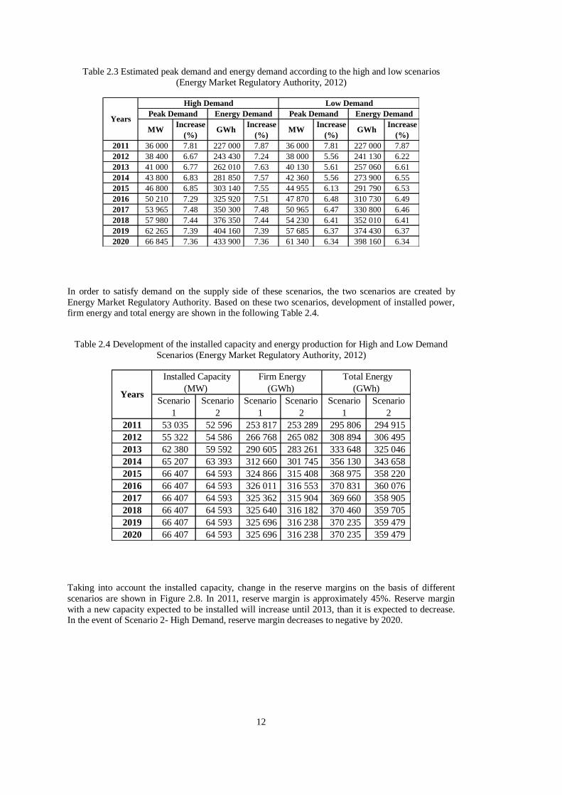
Table 2.3 Estimated peak demand and energy demand according to the high and low scenarios
(Energy Market Regulatory Authority, 2012)
Increase Increase Increase Increase
(%) (%) (%) (%)
2011 36 000 7.81 227 000 7.87 36 000 7.81 227 000 7.87
2012 38 400 6.67 243 430 7.24 38 000 5.56 241 130 6.22
2013 41 000 6.77 262 010 7.63 40 130 5.61 257 060 6.61
2014 43 800 6.83 281 850 7.57 42 360 5.56 273 900 6.55
2015 46 800 6.85 303 140 7.55 44 955 6.13 291 790 6.53
2016 50 210 7.29 325 920 7.51 47 870 6.48 310 730 6.49
2017 53 965 7.48 350 300 7.48 50 965 6.47 330 800 6.46
2018 57 980 7.44 376 350 7.44 54 230 6.41 352 010 6.41
2019 62 265 7.39 404 160 7.39 57 685 6.37 374 430 6.37
2020 66 845 7.36 433 900 7.36 61 340 6.34 398 160 6.34
MW MW GWhGWh
Years
High Demand Low Demand
Peak Demand Energy DemandPeak Demand Energy Demand
In order to satisfy demand on the supply side of these scenarios, the two scenarios are created by
Energy Market Regulatory Authority. Based on these two scenarios, development of installed power, firm energy and total energy are shown in the following Table 2.4.
Table 2.4 Development of the installed capacity and energy production for High and Low Demand
Scenarios (Energy Market Regulatory Authority, 2012)
Scenario Scenario Scenario Scenario Scenario Scenario
1 2 1 2 1 2
2011 53 035 52 596 253 817 253 289 295 806 294 915
2012 55 322 54 586 266 768 265 082 308 894 306 495
2013 62 380 59 592 290 605 283 261 333 648 325 046
2014 65 207 63 393 312 660 301 745 356 130 343 658
2015 66 407 64 593 324 866 315 408 368 975 358 220
2016 66 407 64 593 326 011 316 553 370 831 360 076
2017 66 407 64 593 325 362 315 904 369 660 358 905
2018 66 407 64 593 325 640 316 182 370 460 359 705
2019 66 407 64 593 325 696 316 238 370 235 359 479
2020 66 407 64 593 325 696 316 238 370 235 359 479
Years
Installed Capacity
(MW)
Firm Energy
(GWh)
Total Energy
(GWh)
Taking into account the installed capacity, change in the reserve margins on the basis of different
scenarios are shown in Figure 2.8. In 2011, reserve margin is approximately 45%. Reserve margin
with a new capacity expected to be installed will increase until 2013, than it is expected to decrease. In the event of Scenario 2- High Demand, reserve margin decreases to negative by 2020.

13
Figure 2.8 Development of reserve margins according to installed capacities (Energy Market
Regulatory Authority, 2012)
Given the power generation capacity of power plants, the development of reserve margin is shown in
Figure 2.9. Reserve margin is approximately 30% as of 2011, with the activated capacity in Scenario
1 reserve margin increases until 2013.
Figure 2.9 Reserve margins according to total and firm energy generation capacities (Energy Market
Regulatory Authority, 2012)
Under these circumstances, a serious shortage of electric power supply could be encountered in the
near future. In meeting the energy demand under the circumstances discussed above, it is
indispensable and imperative for Turkey to create additional generation capacity.

14
2.4 Pumped Storage
Pumped storage hydroelectric projects have been providing valuable storage capacity, transmission
grid ancillary benefits and renewable energy in the United States and Europe since the 1920s (Miller, 2010). In other words, pumped storage is a type of hydroelectric power generation that stores energy
in the form of water in an upper reservoir, by pumping from a lower reservoir.
In the power-supply chain, pumped power plant fulfills several important functions as static, dynamic
and compensational (Oliveira, 2011).
i) The static role of the pumped power plant is fulfilled through transformation of surplus energy in
the network into peak energy. At the time when there is a surplus of energy in the network mostly
during the night, the water is pumped from the lower reservoir into the upper one, and in peak
periods, when a shortage of energy occurs, the plant is switched to a turbine mode and it produces
electricity.
ii) The dynamic function of the pumped storage power plant means that the plant functions as a
backup output for the system, it can produce regulatory output and energy and thus it contributes to the administration of the network frequently.
iii) The compensational mode of operation serves for regulating the voltage of the system.
The extend of pumped storage use is very widespread as shown in Figure 2.10, and almost every
industrialized nation can boast at least one such installation.
Figure 2.10 World Pumped Storage Potential (Saraç, 2012)
Turkey needs pumped storage power plants (PSPP) which are all in energy portfolio of developed
countries in a large extend more than any time as parallel to steps taken forward in development of
nuclear power plants and renewable energy generation (Saraç, 2012).
In regards to this, General Directorate of Electrical Power Resources Survey and Development
Administration planned and designed 18 PSPP projects in reconnaissance level and two at pre-

15
feasibility level in 2011. Gökçekaya PSPP, at pre-feasibility level, is planned to be on the Sakarya
River, and Gökçekaya Dam Reservoir is thought to be lower reservoir with an installed capacity of
1400 MW (Saraç, 2012).
Mid century, half of the world energy needs may be supplied at an acceptable cost by wind and sun
but this requires electric energy storage close to 3 000 GW for 50 000 GWh. Pumped storage plants
appear the best relevant solution (Lempérière, 2011).
Lempérière (2011) presented two options below for the future of world energy :
i. Huge utilization of coal, limited however end of the century by the coal availability
as shown in Table 2.5.
ii. Huge utilization of wind and solar energies; it is possible but requires storages of
electric energy as shown in Table 2.5.
Table 2.5 Sources of energy utilization (Lempérière, 2011)
Sources of Energy 2010
(TWh/year)
2050 (option 1)
(based on coal)
(TWh/year)
2050 (option 2)
(based on renewable)
(TWh/year)
Nuclear 3 000 5 000 7 000
Hydro 3 000 5 000 8 000
Biomass, Geotermy,
Miscellaneous 4 000 10 000 15 000
Oil and Gas 40 000 25 000 15 000
Coal 10 000 50 000 15 000
Wind and Solar - 25 000 60 000
Total of Energy
Utilization 60 000 120 000 120 000
There are two types of turbines used in pump storage projects as shown in Figure 2.11. Firstly, the
classic concept with separate machines may be used due to the need for extremely rapid switching time between turbine and pump operation. As two separate hydraulic machines, the rotational
direction of the motor generator can be the same in both operational modes and this solution may add
commercial value to today’s utility operators (Mitteregger, 2008). Secondly, characteristic of
reversible pump-turbines is the longer switch-over time from turbine to pump operation and vice
versa. This is down to the air being used to expel the water in the turbine for restarting under pump
operations, as the start-up equipment for the motor would not be in a position to do so with water. The
rotational direction must also be changed, as this reversible machine operates in both, pump and
turbine mode. In both cases, the selected design for the pumped storage arrangements should be
chosen as an optimum technical solution that results in the best possible return for the operating utility
(Jefferies, 1990).

16
Figure 2.11 Types of pumped turbines (Voith, 2009)
The principal types of pumped storage schemes known today can be classified under four headings, as
shown in Figure 2.12.
i ) Pure pumped storage iii ) Water-transfer type
ii ) Multi-use type iv ) Tidal type

17
Reversible
Pump-turbine
BasinOcean
UPPER RESERVOIR
UPPER RESERVOIR
LOWER RESERVOIR
LOWER RESERVOIR
Reversible
Pump-turbine
Conventional
Turbine
Recirculating type
Multiuse type
Water-transfer type
Tidal type
Figure 2.12 Types of pumped storages development (Voith, 2009)

18
2.5 Mathematical Formulation of the Model
Nandalal and Bogardi (2007) state that simulation is used to analyze the effects of proposed
management plans: achievement regarding system performance is evaluated based on selected sets of decisions. Simulation model is based on the principle of continuity and solves the storage equation in
a specific time. The state of the reservoir system is described by water available in the reservoir at the
beginning of any time step. Consecutive time steps are identified as stages. The decision variable is
water released from the reservoir.
2.5.1 Storage Volume Constraint
The model is operated on daily basis. Since operation policy is derived for annual cycles,
where
S1 = storage volume at beginning of the first period (first day)
ST+1 = storage volume at the end of the last period (last day)
T = total number of time steps (days)
For all other months reservoir storage belongs to the set of admissible storage volume:
where
Sj = storage volume at the beginning period j
Smin = allowable minimum storage volume, and
Smax = allowable maximum storage volume.
2.5.2 Release Constraint
The capacity of hydropower generators sets a maximum limit to reservoir release. If a minimum release request is not considered, the minimum release is set to zero. The release during any day
should be within this feasible release range:
where
Rj = reservoir release during period j, and
Rj,max = maximum allowable release through turbines in period j.
(2.2) 11 TSS
(2.3) maxmin SSS j
(2.4) 0 max,jj RR

19
2.5.3 State Transformation Equation
The state transformation equation based on the principle of continuity is as follows:
where
Ej = evaporation from reservoir during period j
Ij = inflow to the reservoir during period j, and
Qj = spillage water during period j.
Other variables are as defined before.
2.6 Reservoir Simulation Models
Kansal (2005) states that the essence of simulation is to reproduce the behavior of the system from
every point of view to investigate how the system will respond to conditions that may be imposed on
it or that may occur in the future.
Özbakır (2009) made a simulation model of Seyhan and Ceyhan river basins by using the package
HEC-ResSim. He had simulated both Seyhan and Ceyhan river basin models first for existing and
planning scenarios and then for a search in excess water potential of each basin.
Rukuni's (2006) study is about the determination of the impact of small reservoirs on improved and
sustainable rural livelihoods in semi arid regions of Zimbabwe. Water Evaluation and Planning
(WEAP) system model is used to evaluate and simulate the various livelihood issues in the related subcatchment of the basins.
Growth in using simulation models in water management studies makes a good progress in computer
based programs. In the following chapters some common computer based Decision Support Systems
(DSS) are explained.
2.6.1 HEC-5
HEC-5 contains iterative search algorithms for making multiple-reservoir release decisions for each time interval during the simulation of a flood event. Program has optional economic analysis
capabilities for computing expected annual flood damages for different operating plans. HEC-5 also
has extensive capabilities for simulating reservoir operations involving hydroelectric power, water
supply, and low flow augmentation.
2.6.2 WEAP
Water Evaluation and Planning system is a computer-based decision support system for integrated
water resources management. Program was created by Stockholm Environmental Institute in Boston,
Massachusetts. It is used to model simulations of water demand, energy demand, groundwater and
water quality in a reservoir or river system. The analyst can create various models by using script
editor as well (Figure 2.13).
(2.5) 1 jjjjjj QREISS
20
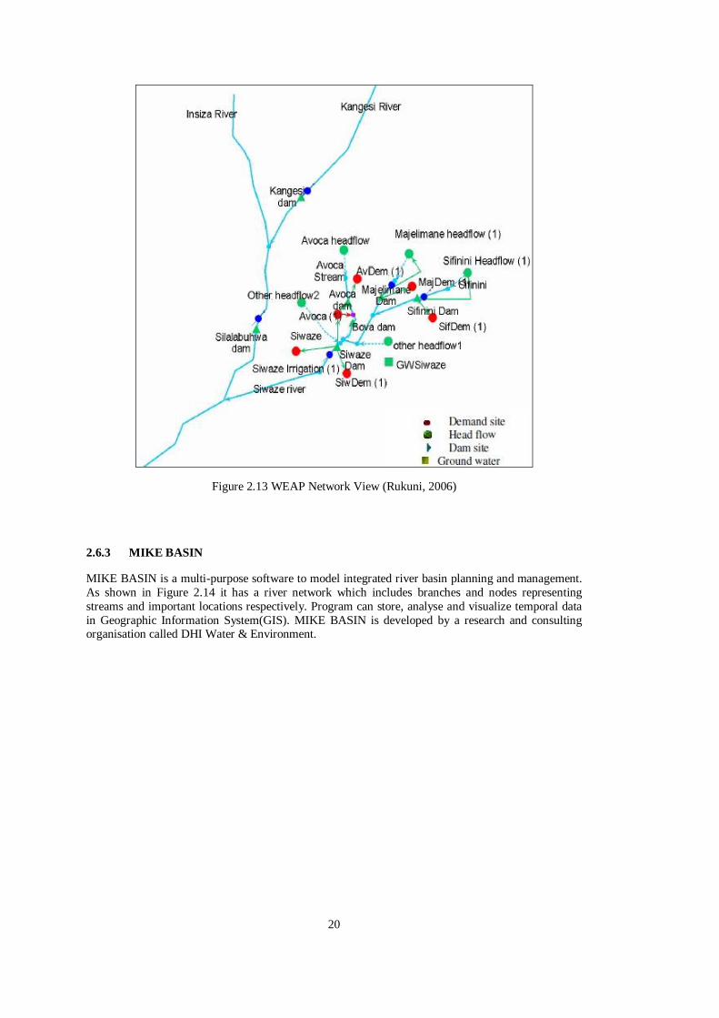
Figure 2.13 WEAP Network View (Rukuni, 2006)
2.6.3 MIKE BASIN
MIKE BASIN is a multi-purpose software to model integrated river basin planning and management.
As shown in Figure 2.14 it has a river network which includes branches and nodes representing
streams and important locations respectively. Program can store, analyse and visualize temporal data
in Geographic Information System(GIS). MIKE BASIN is developed by a research and consulting organisation called DHI Water & Environment.

21
Figure 2.14 MIKE BASIN Network View (University of Texas, 2012)
2.6.4 HEC-ResSim
HEC-ResSim is a freely available reservoir simulation software developed and maintained by the US
Army Corps of Engineers, Hydrologic Engineering Center. The latest release version 3.0 is used
world-wide in many applications, but especially by US environmental and water management
agencies. The software is based on earlier versions of HEC, but now makes use of Java code and
graphical user interfaces.
The basic purpose of the HEC-ResSim model is to simulate the operation of single or multiple
(interconnected) reservoirs. As input, the model requires inflow data to the system. Such data can
represent measurements at stream gauges or be outputs of e.g. precipitation-runoff models. The HEC-
ResSim model is able to handle in an efficient way the analysis of several alternative scenarios. Such
scenarios may differ in the inflow data, the operation rules, reservoir characteristics or the general
reservoir network.
Detailed documentation of the model is available from the HEC-ResSim website which has a manual
consisting of 500 pages. It is recommended to check the website for model updates (Klipsch, 2007).

22

23
CHAPTER 3
2. KALEKÖY CASCADE RESERVOIR SYSTEM
3.1 Description of Watershed
The past three decades have seen a renaissance in the development of the land and water resources of
the anciently civilized river basins of the Middle East. In recent years the Indus Valley of Pakistan, the Nile Valley of Egypt, the Khuzestan of Iran, and the Lower Mesopotamian region of Syria and
Iraq have benefited from river projects on a massive scale which will promote as much economic
growth in present generation as has been achieved in the past four thousand years.
There are two major rivers in the eastern region of Anatolia, the Euphrates and the Tigris. The valley
of these two rivers encompasses the northern portion of the famed and fertile crescent of the
Mesopotamia.
The Fırat (Euphrates) River, the largest river in the Middle-East, originates in the high mountains of Eastern Turkey at an elevation of over 3,000 meters above sea level. The Fırat River has the largest
catchment area of all Turkish rivers, and is composed of two distinct parts: The upper basin and the
lower basin. The upper basin is mountainous and lies above the confluence of the Fırat and the Murat
rivers. The project area is within the catchment area of Murat River which is a tributary of Fırat River.
The principal tributary, the Murat, originates from the skirts of Aladağ in the vicinity of Diyadin
District within the province of Ağrı. As the river continues its flow towards the west, it runs through
the province of Ağrı. At the end of Ağrı Plain, Şeryan Creek joins the river, fed by various tributaries.
Thereafter, Murat River runs through a valley for about 70 km towards the south and passes Malazgirt
and Bulanık plains. The tributaries as Nadirşeyh, Hınıs and Patnos join the river branch. Running
through Alpaslan I dam site where construction was completed, the river is joined by Bingöl Creek.
Then it reaches Alpaslan 2 dam site. In Muş plain, it confluences with Karasu and runs into a deep
valley. Göynük Creek joins the river branch in the vicinity of Genç District. The river continues its flow through the valley and reaches the reservoir of Keban Dam, close to Palu District.
The development of the water resources of the Murat River, has been investigated by the state
agencies through its agencies over many years. The authorities under consideration have developed
projects aimed for irrigation, water supply and energy utilizing the flow data of these stations in order
to develop the water and land resources of Murat River Basin. Some of these projects are under
operation, whereas, some are under construction or in final design, planning, and reconnaissance
stages.
Kaleköy reservoir system lies immediately upstream of Keban, and, from the point of view of size and
cost of power and energy production, it is one of the most attractive hydroelectric projects not only on
the Murat River but in Turkey as a whole. The reservoirs and their locations are given in Figure 3.1.

24
Figure 3.1 Location of the Kaleköy reservoir system on map of Turkey (World Map, 2012)
Figure 3.2 illustrates the layout of the facilities aiming to utilize the hydroelectric potential between
Alpaslan 1 Dam and Keban Dam. Note that, Keban and Alpaslan 1 Dams are in operation stage,
Alpaslan 2 Dam in final design stage, and the others are in feasibility stage. In addition to this, a
schematic diagram of a cascade system is shown in Figure 3.3.
The physical characteristics of the dams, minimum and maximum reservoir operation water levels
have been obtained identically from the Feasibility Report (Temelsu International Engineering
Services Inc., 2011).

25
Figure 3.2 Hydropower plants’ layout in the basin (Temelsu International Engineering Services Inc., 2011)
25

26
Figure 3.3 Schematic diagram of Kaleköy reservoir system
26

27
Limitation of the tailwater levels, as well as the topography of the region, geological conditions affect dam axes locations and operation water levels as mentioned in Feasibility Report (2011).
Hydroelectric potential between the elevations of 1225 m and 870 m for Murat tributary was divided
in two stages. These two stages compose the upstream part between the elevations of 1225 m and
1020 m and the downstream part between the elevations of 1020 m and 870 m. Settlement areas and
irrigation areas specify the boundaries of the stages as shown in Figure 3.4. The maximum water
elevation at the upstream part has been specified as 1225 m depending on the irrigation and drainage
of Muş Plain, whereas the tailwater level has been specified as 1020 m depending on the elevation of
Bingöl Plain. At the Kaleköy reservoir system downstream part, maximum water elevation has been
specified as 982 m depending on the layout of Genç District. Tailwater elevation at the downstream
part has been accepted as 870 m.
For the purpose of utilizing the means of energy offered by Murat River between the elevations of
870-1225 m, the main facilities from the upstream towards the downstream are a series of four dams
listed as follows:
i) Upper Kaleköy Dam and HEPP
ii) Lower Kaleköy Dam and HEPP
iii) Beyhan 1 Dam and HEPP
iv) Beyhan 2 Dam and HEPP
It has been accepted that the Kaleköy reservoir system would have been completed and commissioned
in 2015.
3.2 Installed Capacity
The first step in any system analysis study is to identify the hydrologic and physical features of the system.
The powerplant installed capacity establishes an upper limit on the amount of energy that can be
generated in a period. The installed capacities of Upper Kaleköy HEPP, Lower Kaleköy HEPP,
Beyhan 1 HEPP and Beyhan 2 HEPP have been determined as 600 MW, 450 MW, 550 MW, 255
MW, respectively by the owner based on the decision of General Directorate of Electrical Power
Resources.
The upstream development facilities existing or planned to be constructed on Murat River and its
tributaries are directly related with this project only in terms of water supply. The water requirements
and water consumptions of the projects developed for the purposes of water supply and irrigation at
the upstream of the proposed facilities have been analysed in two steps as for the existing and future
cases. The effect of these water requirements on the inflows of the Kaleköy reservoir system has been taken into account and the inflows of the facilities have been calculated in Feasibility Report
(Temelsu International Engineering Services Inc., 2011).

28
PALU VILLAGE
MUS PLAIN
905.00 902.00
910.00
987.00
1107.50
1230.00
982.00
1102.50
1225.00
SEDIMENT VOLUME (10 m)6 3
218.0
(10 m)6 3
INACTIVE VOLUME 406.2
ACTIVE VOLUME (10 m)6 3
189.1
(m)
(m)
MAXIMUM OPERATION WATER LEVEL
MINIMUM OPERATION WATER LEVEL
1225.0
1210.0
(m)
INSTALLED POWER (MW)
GROSS HEAD 122.5
600.0
TOTAL VOLUME OF RESERVOIR
HEIGHT (FROM THALWEG) (m)
(10 m)6 3
SEDIMENT VOLUME (10 m)6 3
(10 m)6 3
INACTIVE VOLUME
ACTIVE VOLUME (10 m)6 3
(m)
(m)
MAXIMUM OPERATION WATER LEVEL
MINIMUM OPERATION WATER LEVEL
(m)
INSTALLED POWER (MW)
GROSS HEAD
TOTAL VOLUME OF RESERVOIR
HEIGHT (FROM THALWEG) (m)
(10 m)6 3
SEDIMENT VOLUME (10 m)6 3
(10 m)6 3
INACTIVE VOLUME
ACTIVE VOLUME (10 m)6 3
(m)
(m)
MAXIMUM OPERATION WATER LEVEL
MINIMUM OPERATION WATER LEVEL
(m)
INSTALLED POWER (MW)
GROSS HEAD
41.8
35.0
255.0
0.0
905.0
902.0
63.55
15.37
78.92TOTAL VOLUME OF RESERVOIR
HEIGHT (FROM THALWEG) (m)
(10 m)6 3
SEDIMENT VOLUME (10 m)6 3
(10 m)6 3
INACTIVE VOLUME
ACTIVE VOLUME (10 m)6 3
(m)
(m)
MAXIMUM OPERATION WATER LEVEL
MINIMUM OPERATION WATER LEVEL
(m)
INSTALLED POWER (MW)
GROSS HEAD
BINGÖL PLAIN
to KEBAN DAM
977.00
1085.00
1210.00
1250
BEYHAN 2 DAM AND HEPP
1200
1150
1100
1050
1000
950
900
850
KM
0+
000.0
00
KM
19+
500.0
00
KM
65+
000.0
00
KM
104+
000.0
00
BEYHAN 1 DAM AND HEPP
83.6
77.0
550.0
982.0
977.0
294.64
74.42
369.06
121.0
LOWER KALEKÖY DAM AND HEPP
90.2
82.5
450.0
1102.5
1085.0
240.10
191.40
431.50
38.0
UPPER KALEKÖY DAM AND HEPP
TOTAL VOLUME OF RESERVOIR
HEIGHT (FROM THALWEG) (m)
(10 m)6 3
127.5
595.3
GENÇ VILLAGE
Figure 3.4 Profile of Kaleköy reservoir system
28
PALU CITY
GENÇ CITY

29
3.3 Hydrology
For a feasible decision on the size of the works, it is important to know the available river discharges
at each dam site for a long period.
The flow through the Fırat basin varies from year to year. A summary of the hydrology of the
Kaleköy reservoir system is given in this chapter. More detailed information is available in the
Feasibility Report (Temelsu International Engineering Services Inc., 2011).
The greater part of the precipitation occurs between November and May and in the higher areas generally falls as snow from the beginning of December and sometimes as early as November. This
snow accumulates during the winter and melts in April and May and, in conjunction with rainfall,
produces the largest floods.
For the purpose of developing the water and land resources of the Murat River Basin, hydrometric stations were installed by the DSİ and EİE Administration on Murat River and its tributaries on
various dates. Daily precipitation observations are carried out at all of the meteorological stations. In
addition to this, other meteorological observations such as temperature, evaporation, relative
humidity, wind, radiation are also recorded at some of the stations.
Murat River and its tributaries are the resource of water in the study area. The catchment areas of
Murat River at the axis locations of Beyhan 2, Beyhan 1, Lower Kaleköy and Upper Kaleköy dams
are, respectively; 25 426 km², 25 274 km², 22 243 km² and 21 337 km².
In this study, the operation studies have been performed in two stages on the basis of monthly flows obtained from Feasibility Report (Temelsu International Engineering Services Inc., 2011):
i) “Existing Case Inflows”
The case illustrating the full development of the irrigation projects existing at the upstream, or the irrigation projections of the projects put under operation, on the date of 2015.
ii) “Full Development Case Inflows”
The case illustrating the commissioning of all existing and future upstream projects with or without
dams and aiming water supply, irrigation and energy production, and also illustrating the full development of their irrigation schemes.
The installed capacity and total energy production for Kaleköy reservoir system have been
determined, taking the projects either existing or planned to be constructed at the upstream, into
account. Accordingly, the flow series of the dams with big reservoirs (storage volumes) either existing
or planned to be constructed at the upstream have been updated, operation studies have been carried
out in Feasibility Report (Temelsu International Engineering Services Inc., 2011).
For a series of hydroelectric stations such as those envisaged on the Lower Murat, the useful
discharges for each of the plants are composed of the following elements:
i) the inflows from the intermediate catchment area situated between the plant under
consideration and that immediately upstream,
ii) the discharge of the plant situated directly upstream,
iii) the losses due to evaporation from the surface of the reservoir.
3.3.1 Climate
Continental climate is dominant within the catchment area of Murat River. The characteristics of this
climate reveal that winters are cold and rainy, summers are hot and dry. Precipitation and temperature
values are taken from Table 3.1.
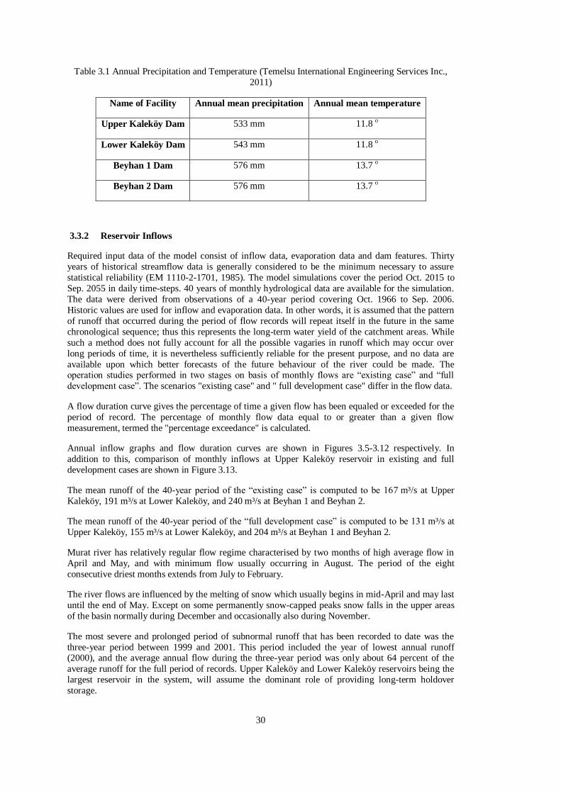
30
Table 3.1 Annual Precipitation and Temperature (Temelsu International Engineering Services Inc.,
2011)
Name of Facility Annual mean precipitation Annual mean temperature
Upper Kaleköy Dam 533 mm 11.8 o
Lower Kaleköy Dam 543 mm 11.8 o
Beyhan 1 Dam 576 mm 13.7 o
Beyhan 2 Dam 576 mm 13.7 o
3.3.2 Reservoir Inflows
Required input data of the model consist of inflow data, evaporation data and dam features. Thirty
years of historical streamflow data is generally considered to be the minimum necessary to assure
statistical reliability (EM 1110-2-1701, 1985). The model simulations cover the period Oct. 2015 to
Sep. 2055 in daily time-steps. 40 years of monthly hydrological data are available for the simulation.
The data were derived from observations of a 40-year period covering Oct. 1966 to Sep. 2006.
Historic values are used for inflow and evaporation data. In other words, it is assumed that the pattern
of runoff that occurred during the period of flow records will repeat itself in the future in the same
chronological sequence; thus this represents the long-term water yield of the catchment areas. While
such a method does not fully account for all the possible vagaries in runoff which may occur over
long periods of time, it is nevertheless sufficiently reliable for the present purpose, and no data are
available upon which better forecasts of the future behaviour of the river could be made. The operation studies performed in two stages on basis of monthly flows are “existing case” and “full
development case”. The scenarios "existing case" and " full development case" differ in the flow data.
A flow duration curve gives the percentage of time a given flow has been equaled or exceeded for the
period of record. The percentage of monthly flow data equal to or greater than a given flow
measurement, termed the "percentage exceedance" is calculated.
Annual inflow graphs and flow duration curves are shown in Figures 3.5-3.12 respectively. In
addition to this, comparison of monthly inflows at Upper Kaleköy reservoir in existing and full
development cases are shown in Figure 3.13.
The mean runoff of the 40-year period of the “existing case” is computed to be 167 m³/s at Upper
Kaleköy, 191 m³/s at Lower Kaleköy, and 240 m³/s at Beyhan 1 and Beyhan 2.
The mean runoff of the 40-year period of the “full development case” is computed to be 131 m³/s at
Upper Kaleköy, 155 m³/s at Lower Kaleköy, and 204 m³/s at Beyhan 1 and Beyhan 2.
Murat river has relatively regular flow regime characterised by two months of high average flow in
April and May, and with minimum flow usually occurring in August. The period of the eight
consecutive driest months extends from July to February.
The river flows are influenced by the melting of snow which usually begins in mid-April and may last
until the end of May. Except on some permanently snow-capped peaks snow falls in the upper areas
of the basin normally during December and occasionally also during November.
The most severe and prolonged period of subnormal runoff that has been recorded to date was the
three-year period between 1999 and 2001. This period included the year of lowest annual runoff (2000), and the average annual flow during the three-year period was only about 64 percent of the
average runoff for the full period of records. Upper Kaleköy and Lower Kaleköy reservoirs being the
largest reservoir in the system, will assume the dominant role of providing long-term holdover
storage.

31
0
500
1000
1500
2000
2500
3000
3500
4000
4500
5000
5500
6000
6500
7000
7500
8000
8500
9000
9500
10000
10500
11000
19
67
19
68
19
69
19
70
19
71
19
72
19
73
19
74
19
75
19
76
19
77
19
78
19
79
19
80
19
81
19
82
19
83
19
84
19
85
19
86
19
87
19
88
19
89
19
90
19
91
19
92
19
93
19
94
19
95
19
96
19
97
19
98
19
99
20
00
20
01
20
02
20
03
20
04
20
05
20
06
An
nu
al F
low
( h
m³
)
Reservoir Inflow
Figure 3.5 Annual inflow of Upper Kaleköy reservoir in existing case
0
50
100
150
200
250
300
350
% 0 % 10 % 20 % 30 % 40 % 50 % 60 % 70 % 80 % 90 % 100
Percentage of Time Flow Exceeded
An
nu
al
Flo
w (
m³/
s)
duration curve average
Figure 3.6 Annual flow duration curve of Upper Kaleköy reservoir in existing case
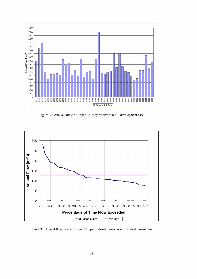
32
0
500
1000
1500
2000
2500
3000
3500
4000
4500
5000
5500
6000
6500
7000
7500
8000
8500
9000
9500
19
67
19
68
19
69
19
70
19
71
19
72
19
73
19
74
19
75
19
76
19
77
19
78
19
79
19
80
19
81
19
82
19
83
19
84
19
85
19
86
19
87
19
88
19
89
19
90
19
91
19
92
19
93
19
94
19
95
19
96
19
97
19
98
19
99
20
00
20
01
20
02
20
03
20
04
20
05
20
06
An
nu
al
Flo
w (
hm
³ )
Reservoir Inflow
Figure 3.7 Annual inflow of Upper Kaleköy reservoir in full development case
0
50
100
150
200
250
300
% 0 % 10 % 20 % 30 % 40 % 50 % 60 % 70 % 80 % 90 % 100
Percentage of Time Flow Exceeded
An
nu
al
Flo
w (
m³/
s)
duration curve average
Figure 3.8 Annual flow duration curve of Upper Kaleköy reservoir in full development case

33
0
200
400
600
800
1000
1200
1400
1600
1800
2000
19
67
19
68
19
69
19
70
19
71
19
72
19
73
19
74
19
75
19
76
19
77
19
78
19
79
19
80
19
81
19
82
19
83
19
84
19
85
19
86
19
87
19
88
19
89
19
90
19
91
19
92
19
93
19
94
19
95
19
96
19
97
19
98
19
99
20
00
20
01
20
02
20
03
20
04
20
05
20
06
An
nu
al
Flo
w (
hm
³ )
Reservoir Inflow
Figure 3.9 Annual intermediate inflow between Upper Kaleköy reservoir and Lower Kaleköy
reservoir in existing and full development case
0
10
20
30
40
50
60
70
% 0 % 10 % 20 % 30 % 40 % 50 % 60 % 70 % 80 % 90 % 100
Percentage of Time Flow Exceeded
An
nu
al
Flo
w (
m³/
s)
duration curve average
Figure 3.10 Annual flow duration curve of intermediate inflow between Upper Kaleköy and Lower
Kaleköy reservoir in existing and full development case

34
0
500
1000
1500
2000
2500
3000
3500
1967
1968
1969
1970
1971
1972
1973
1974
1975
1976
1977
1978
1979
1980
1981
1982
1983
1984
1985
1986
1987
1988
1989
1990
1991
1992
1993
1994
1995
1996
1997
1998
1999
2000
2001
2002
2003
2004
2005
2006
An
nu
al
Flo
w (
hm
³ )
Reservoir Inflow
Figure 3.11 Annual intermediate inflow between Lower Kaleköy reservoir and Beyhan 1 reservoir in
existing and full development case
0
20
40
60
80
100
120
% 0 % 10 % 20 % 30 % 40 % 50 % 60 % 70 % 80 % 90 % 100
Percentage of Time Flow Exceeded
An
nu
al
Flo
w (
m³/
s)
duration curve average
Figure 3.12 Annual flow duration curve of intermediate inflow between Lower Kaleköy reservoir and
Beyhan 1 reservoir in existing and full development case

35
0.0
200.0
400.0
600.0
800.0
1000.0
1200.0
1400.0
Oct-
66
Oct-
67
Oct-
68
Oct-
69
Oct-
70
Oct-
71
Oct-
72
Oct-
73
Oct-
74
Oct-
75
Oct-
76
Oct-
77
Oct-
78
Oct-
79
Oct-
80
Oct-
81
Oct-
82
Oct-
83
Oct-
84
Oct-
85
Oct-
86
Oct-
87
Oct-
88
Oct-
89
Oct-
90
Oct-
91
Oct-
92
Oct-
93
Oct-
94
Oct-
95
Oct-
96
Oct-
97
Oct-
98
Oct-
99
Oct-
00
Oct-
01
Oct-
02
Oct-
03
Oct-
04
Oct-
05
Flo
w (
m³/
s)
existing case full development
Figure 3.13 Comparison of monthly inflow at Upper Kaleköy reservoir in existing and full development case
35

36
3.3.3 Environmental Flows
When hydraulic structures are constructed on a river to regulate water, environmental flow is the
minimum water regime to maintain ecosystems and their benefits (Dyson et al., 2003). Environmental flows based on the feasibility report prepared by Temelsu Inc., Turkey in 2011 are shown in Table
3.2.
Environmental flow in wet season (march, april, may, june) approximately equals to 20 percent of the
annual average flow, in dry season it equals to 10 percent of the annual average flow. However,
environmental flows should be set on the basis of the needs of the downstream reach and not simply
from a formula whether related to average flow or the flow duration curve.
Table 3.2 Environmental Flows
Upper Kaleköy Lower Kaleköy Beyhan 1 Beyhan 2
January 17.73 20.15 37.50 37.50
February 17.73 20.15 37.50 37.50
March 35.45 40.31 50.00 50.00
April 35.45 40.31 50.00 50.00
May 35.45 40.31 50.00 50.00
June 35.45 40.31 50.00 50.00
July 17.73 20.15 37.50 37.50
August 17.73 20.15 37.50 37.50
September 17.73 20.15 37.50 37.50
October 17.73 20.15 37.50 37.50
November 17.73 20.15 37.50 37.50
December 17.73 20.15 37.50 37.50
MonthQenv (m³/s)
3.3.4 Trends in River Flow
The flow data shows that flows have been significantly below the long term average in recent years.
The average flow over the past 10 years is about 91% of the long term average. It is not clear whether
this is a result of natural variation or some long-term trend, but it would be prudent to consider the
impact of lower flows on power generation.
The pattern of average monthly flows for the Murat at Upper Kaleköy is shown in Figure 3.13, from
which the following hydrological conditions were deduced in the existing case:
Average flow in the driest month (November 2002) 39.8 m³/s
Average flow in the driest year (2000) 95.1 m³/s
Average flow in the driest 3-year period (1999 - 2001) 106.0 m³/s
Average flow over the 40 years (1966 - 2006) 167 m³/s
Average flow over the 10 years (1996 - 2006) 152.23 m³/s
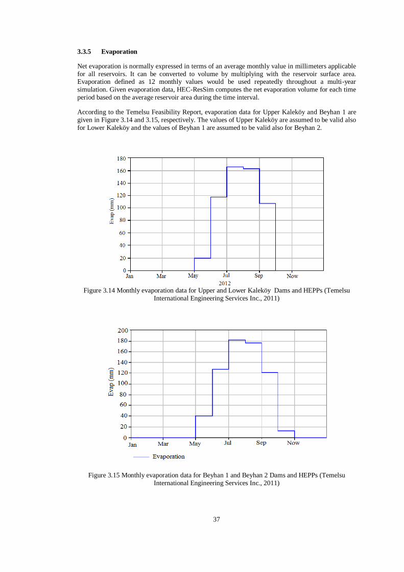
37
3.3.5 Evaporation
Net evaporation is normally expressed in terms of an average monthly value in millimeters applicable
for all reservoirs. It can be converted to volume by multiplying with the reservoir surface area. Evaporation defined as 12 monthly values would be used repeatedly throughout a multi-year
simulation. Given evaporation data, HEC-ResSim computes the net evaporation volume for each time
period based on the average reservoir area during the time interval.
According to the Temelsu Feasibility Report, evaporation data for Upper Kaleköy and Beyhan 1 are
given in Figure 3.14 and 3.15, respectively. The values of Upper Kaleköy are assumed to be valid also
for Lower Kaleköy and the values of Beyhan 1 are assumed to be valid also for Beyhan 2.
Figure 3.14 Monthly evaporation data for Upper and Lower Kaleköy Dams and HEPPs (Temelsu
International Engineering Services Inc., 2011)
Figure 3.15 Monthly evaporation data for Beyhan 1 and Beyhan 2 Dams and HEPPs (Temelsu
International Engineering Services Inc., 2011)

38
3.3.6 Sediment Yield
When Kaleköy reservoir system is under operation, Alpaslan I Dam will be under operation too. For
this reason, Alpaslan I Dam will control the sediment volume expected from its own basin. Dead
volume for each reservoir is calculated according to the 50 years operation period in Feasibility
Report (Temelsu International Engineering Services Inc., 2011). Values in Table 3.3 are directly
obtained from the same report.
Vortex effect limits operation water level as minimum. Whether the submergence provided at the minimum water level is sufficient or not is checked in order to avoid vortex formation in front of the
intake structure. Several formulas have been developed that define the submergence required.
For a recommended method for computing submergence requirements at well operating prototypes,
ASCE (1995) provided a graph as shown in Figure 3.16. The recommendations are valid for intakes
with proper approach flow conditions. An example calculation for Beyhan 2 Dam’s intake structure is
presented below.
Where
Fr = Froude number = 5.71/(9.81*7.80)0.5 = 0.653
Q = turbined flow = 272.90 m³/s
D = diameter of the penstock = 7.80 m = 25.584 ft
A = area of the penstock = 47.78 m²
V = velocity of the flow = 272.90/47.78 = 5.71 m/s = 18.73 ft/s
\
where
h = Submergence depth is defined as the distance between minimum water level and centerline
of intake
h/D = 2*0.653 + 0.5
h = 1.806*7.8 = 14.1 m
Existing Submergence = 902.00 – 878.90 = 23.1 m > 14.1 m
Table 3.3 Sediment volumes of reservoirs
Name of
Facility
Dead storage Dead storage Invert elevation of Minimum operation
volume height intake structure water level
(hm³) (m) (m) (m)
Upper Kaleköy 218.0 1189.0 1190.0 1210.0
Lower Kaleköy 38.0 1048.0 1069.0 1085.0
Beyhan 1 121.0 962.0 962.0 977.0
Beyhan 2 0.0 868.2 875.0 902.0
(3.1) .Dg
VFr
(3.2) 2/12 rFh

39
Figure 3.16 Recommended submergence for intakes (ASCE, 1995)
3.4 Reservoir Storage
Reservoirs are defined by a series of relationships based on storage. The storage against maximum
outflow relationship is required. For conservation studies, reservoir areas are needed for evaporation
computation and elevations are needed for hydropower computations. Both area and elevation are
given as functions of storage.
The elevation-area curves for the dam in Kaleköy reservoir system is given in Figures 3.17 - 3.20.
1100
1110
1120
1130
1140
1150
1160
1170
1180
1190
1200
1210
1220
1230
1240
1250
0 50 100 150 200 250 300 350 400 450 500 550 600 650 700 750 800 850 900 950
Volume (hm3)
Ele
vatio
n (
m)
0.0010.0020.0030.0040.00
Area (km2)

40
Figure 3.17 Elevation-area curve for Upper Kaleköy Dam (Temelsu International Engineering
Services Inc., 2011)
1015
1025
1035
1045
1055
1065
1075
1085
1095
1105
1115
0 50 100 150 200 250 300 350 400 450 500 550
Volume (hm3)
Ele
vation (
m)
0.002.505.007.5010.0012.5015.00
Area (km2)
Figure 3.18 Elevation-area curve for Lower Kaleköy Dam (Temelsu International Engineering
Services Inc., 2011)
900
910
920
930
940
950
960
970
980
990
0 50 100 150 200 250 300 350 400 450 500 550 600
Volume (hm3)
Ele
vation (
m)
0.006.0012.0018.0024.0030.0036.00
Area (km2)
Figure 3.19 Elevation-area curve for Beyhan 1 Dam (Temelsu International Engineering Services Inc.,
2011)

41
865
875
885
895
905
915
0 10 20 30 40 50 60 70 80 90 100 110
Volume (hm3)
Ele
va
tio
n (
m)
0.002.004.006.00
Area (km2)
Figure 3.20 Elevation-area curve for Beyhan 2 Dam (Temelsu International Engineering Services Inc.,
2011)
3.5 Tailwater Rating Curves
The tailwater may be specified as a constant value or with a rating curve. If a downstream lake
elevation could affect the tailwater elevation, the program can check that elevation to see if it is higher
than the block loading tailwater elevation or the tailwater rating curve. If it is, then the downstream
lake elevation would be used. When two or more ways are used to describe the tailwater, the higher
tailwater is used.
Tailwater elevation is a function of the total project discharge, the outlet channel geometry, and
backwater effects and is represented by a tailwater rating curve.
Developing a curve for tailwater elevation versus river discharge can be the source of a great deal of
field work. A way of developing a tailwater curve for a given site; is to develop the curve from the
computed backwater curve, i.e., HECRAS 4.1, developed by the Hydraulic Engineering Center (HEC), U.S. Army Corps of Engineers, Davis, California.
The tailwater rating curves for all the dam sites are given in Figures 3.21-3.23 respectively.

42
1102.0
1103.0
1104.0
1105.0
1106.0
1107.0
1108.0
0.0 250.0 500.0 750.0 1000.0 1250.0 1500.0 1750.0 2000.0
Q (m3/s)
Tail
wate
r L
evels
(m
)
Figure 3.21 Tailwater rating curve for the dam site of Upper Kaleköy
1017.0
1018.0
1019.0
1020.0
1021.0
1022.0
1023.0
1024.0
0 200 400 600 800 1000 1200 1400 1600 1800
Q (m3/s)
Tail
wate
r L
evels
(m
)
Figure 3.22 Tailwater rating curve for the dam site of Lower Kaleköy

43
904.5
905.0
905.5
906.0
906.5
907.0
907.5
908.0
908.5
909.0
909.5
910.0
0.0 250.0 500.0 750.0 1000.0 1250.0 1500.0 1750.0 2000.0
Q (m3/s)
Ta
ilw
ate
r L
ev
els
(m
)
Figure 3.23 Tailwater rating curve for the dam site of Beyhan 1
869.5
870.0
870.5
871.0
871.5
872.0
872.5
873.0
873.5
0.0 250.0 500.0 750.0 1000.0 1250.0 1500.0 1750.0 2000.0
Q (m3/s)
Ta
ilw
ate
r L
ev
els
(m
)
Figure 3.24 Tailwater rating curve for the dam site of Beyhan 2

44
3.6 Head Losses
In determining the net head available for power generation, it is necessary to account for head loss in
the water passages. These losses include primarily friction losses in the trashrack, intake structure, and penstock. Hydraulic losses between the entrance to the turbine and the draft tube exit are accounted
for in the turbine efficiency. Head losses for Upper Kaleköy, Lower Kaleköy, Beyhan 1 and Beyhan 2
dams are 2.5 m, 1.0 m, 2.0 m and 1.0 m respectively (Temelsu International Engineering Services
Inc., 2011). Friction, entrance, trashrack, gate, transition and curvature losses are the main hydraulic
losses taken into account.
3.7 Efficiency
When calculating the power and energy output of each plant, the gross head was determined day by day as the difference between reservoir and tailwater level. Efficiencies in the hydraulic system,
estimated for average conditions and the same for each plant, are deducted, by assuming the following
efficiencies for operation under average conditions:
e = overall plant efficiency = e turbine x e generator x e transformer (3.3)
e = 0.92 x 0.98 x 0.99 = 0.893 (Temelsu International Engineering Services Inc., 2011)
3.8 Dams’ Features
The characteristics of the reservoir system are defined by a number of parameters that are described below in brief.
3.8.1 Upper Kaleköy Dam and HEPP
Upper Kaleköy dam is located just at the downstream of the confluence of Murat River and Karasu and its catchment area is 21 337 km². The annual mean flow at Upper Kaleköy dam site for this period
is 5590 hm³.
A hydroelectric power plant with an installed capacity of 600 MW will be constructed by the roller
compacted concrete at the location shown in Figure 3.4 with a height of 127.5 m from the thalweg and
150.0 m from the foundation. The power plant has three main and one small Francis type of turbines.
The maximum operation water level of Upper Kaleköy Dam has been selected as 1225.0 m by taking
the irrigation and drainage system elevation of Muş-Arıncık Irrigation Project into account. Crest
elevation of the dam is 1230.0 m. The minimum operation water elevation is 1210.0 m. The characteristics of Upper Kaleköy Dam and HEPP is given in Appendix B.
The general plan and typical cross section of Upper Kaleköy Dam and HEPP are shown in Appendix
B.
3.8.2 Lower Kaleköy Dam and HEPP
Lower Kaleköy dam is located at the downstream of Upper Kaleköy dam site and its catchment area is
22 243 km². The annual mean flow at Lower Kaleköy dam site for this period is 6356 hm³.
A hydroelectric power plant with a capacity of 450 MW is installed by the roller compacted concrete
type at the location shown in Figure 3.4 with a height of 90.2 m from the thalweg and 102.5 m from
the foundation.
The maximum operation water level of Lower Kaleköy Dam is defined by the tailwater level of Upper
Kaleköy Dam and HEPP. For this reason, the maximum water elevation has been specified as 1102.5 m. Crest elevation of the dam is 1107.5 m. The minimum operation water elevation is 1085.0 m.
The spillway has been located at right bank as overflow type with gates. The spillway crest elevation,
whose dimensions have been computed according to the probable maximum flood peak discharge, is

45
1087.0 m. The characteristics of Lower Kaleköy Dam and HEPP is given in Appendix B. The general
lan and typical cross section of Lower Kaleköy Dam and HEPP are shown in Appendix B.
3.8.3 Beyhan 1 Dam and HEPP
A hydroelectric power plant with a capacity of 400 MW is installed at the location shown in Figure
3.3 with a height of 83.6 m from the thalweg and 97.0 m from the foundation.
The settlement area of Genç District defines the maximum operation water level of Beyhan 1 Dam. The maximum water level elevation is 982.0 m so that the settlement areas in Genç District are not
inundated. Crest elevation of the dam is 987.0 m. The minimum operation water elevation is 977.0 m
as a result of the sediment estimation.
The spillway has been located at left bank apart from the dam body as overflow type with gates. The
spillway crest elevation, whose dimensions have been computed according to the probable maximum
flood peak discharge, is 967.0 m.
Beyhan 2 and Beyhan 1 dams are the two successive dams located on Murat River. Their catchment
areas are 25 426 km2 and 25 274 km2, respectively. The annual mean flows of Beyhan 2 and Beyhan
1 dams for this period is 7884 hm³. The characteristics of Beyhan 1 Dam and HEPP is given in
Appendix B. The general plan and typical cross section of Beyhan 1 Dam and HEPP are shown in
Appendix B.
3.8.4 Beyhan 2 Dam and HEPP
Beyhan 2 dam site is located on Murat River at the thalweg elevation of 868.2 m. The dam site is located at an air distance of 5.5 km in the east of Palu district center and at the 8th km of the 22 km
long provincial road between Palu-Beyhan. The annual mean flow of Murat River at Beyhan 2 dam
site is 7884 hm³.
A hydroelectric power plant with a capacity of 255 MW is installed by the concrete gravity at the
location shown in Figure 3.3 with a height of 41.8 m from the thalweg and 62,0 m from the
foundation. The power plant has three main and one small Francis type of turbines.
The maximum operation water level of Beyhan 2 Dam is defined by the tailwater level of Beyhan 1 Dam and HEPP. For this reason, the maximum water elevation has been specified as 905.0 m. Crest
elevation of the dam is 910,0 m. The characteristics of Beyhan 2 Dam and HEPP is given in Appendix
B. The general plan and typical cross section of Beyhan 2 Dam and HEPP are shown in Appendix B.
An overview over the most relevant modelling components used for simulation in the Lower Murat
Basin are presented below.

46
3.9 Model Components in HEC-ResSim
A large number of different modelling components are available in HEC-ResSim. This enables the
modeller to build an adequate representation of the system to be studied. For different studies, different modelling components will become important. For instance, in the flood study river routing
and detailed spillway characteristics are important, whereas in the reservoir simulation study
diversions, water requirements and evaporation are important. The current study focuses on the
general simulation of the reservoirs as well as the impact of the reservoirs on energy generation.
The scenarios also have different modelling time-steps. Daily time intervals are the maximum
possible length of modelling time-steps in HEC-ResSim. Therefore, the available monthly inflow data
in the Lower Murat basin are treated as daily values that do not vary within a month. The simulation
period covers 40 years in daily time-steps. Due to the discrete computational time-steps, numerical artefacts may occur, which can cause jumps in the simulated values between months. However, these
numerical artefacts are in general negligible.
An important feature of HEC-ResSim is that the model is divided into three separate sets of functions
called modules:
i) Watershed Setup Module
ii) Reservoir Network Module
iii) Simulation Module
Figure 3.25 provides a graphical illustration of the three modules that constitute HEC-ResSim.
Figure 3.25 HEC-ResSim Module concepts (Klipsch, 2007)

47
The river network, based on the stream alignment, is represented by computation points that are
connected by reaches. This structure defines the topology, such that the model knows in which
direction the water flows as well as where the confluences of separate rivers are located. Intermediate
basin inflows can be specified for each computation point. Similarly, upstream net water
consumptions can be accounted for by subtracting water from river runoff at computation points.
Several different methods for routing of runoff through the reaches between computation points are
available. However, this is generally used in the flood studies, runoff routing is not important for the
reservoir simulation study, which is based on monthly data.
Reservoirs are added upon the stream alignment. In HEC-ResSim model, a large number of properties
for the reservoir can be specified. Some of these include:
i) elevation-area-storage curves
ii) evaporation
iii) outlets
iv) operation rules
The elevation-area-storage curve defines the basic properties of the reservoir for the mass balance
accounting between inflows and outflows. This curve is also used for determining the evaporation
from the surface area of the water body. The water level affects the energy generation as well as the
spillway losses. Further, the operation rules are based upon the water level.
Outlets can represent power plants, diverted outlet, controlled or uncontrolled spillways, outlets for
environmental flow, etc. Power plant specifications include design discharge, tailwater levels,
efficiencies, hydraulic losses. Spillway properties are usually defined by a curve giving the
relationship between water level in the reservoir and spillway discharge. As there may be several
outlets at each reservoir, it is important to specify rules for prioritizing the allocation of water. There
would not be a conflicting demand between diversion of water and environmental flow releases by
specifying rules.
Operation rules are defined for different storage zones in the reservoir. Such operation rules can
represent rules for diversion of water, environmental flow release, or downstream water requirements.
The storage of a reservoir is typically split into three parts: inactive zone (dead zone), conservation
zone, and flood control zone. A guide curve for the operation of the reservoir is implemented by
specifying a seasonal variation in the elevation of the conservation zone. In the simulation, the model
will preferentially try to keep the reservoir water level at the top of the conservation zone, while
obeying all rules like downstream water requirements. If the water level reaches a different zone, then
a different set of rules comes into effect.
3.10 Model Set-up of HEC-ResSim
The HEC-ResSim model is set-up to simulate the operation of the reservoirs in the Lower Murat
basin.
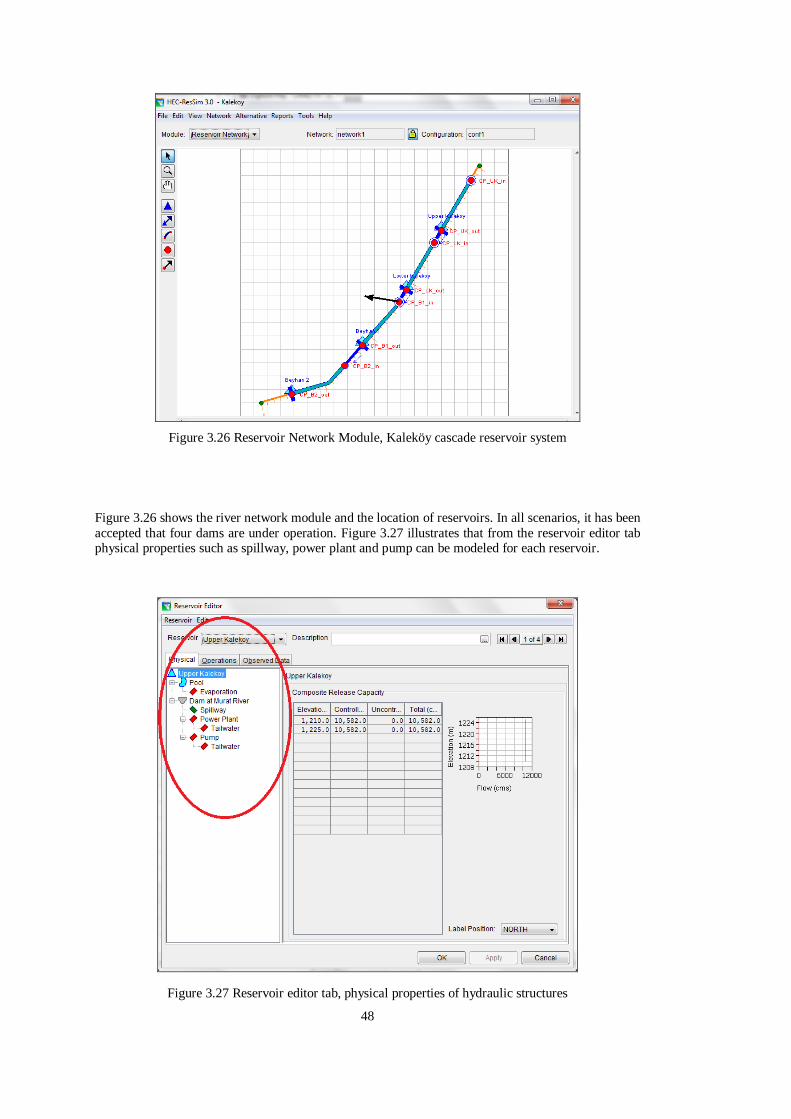
48
Figure 3.26 Reservoir Network Module, Kaleköy cascade reservoir system
Figure 3.26 shows the river network module and the location of reservoirs. In all scenarios, it has been
accepted that four dams are under operation. Figure 3.27 illustrates that from the reservoir editor tab physical properties such as spillway, power plant and pump can be modeled for each reservoir.
Figure 3.27 Reservoir editor tab, physical properties of hydraulic structures

49
Different types of rules are available for specifying the operation of the reservoir depending on the
storage zone. Basic rules representing environmental flows and firm energy requirements are
implemented as shown in Figure 3.28.
Figure 3.28 Reservoir Editor, operating rules
Environmental flow releases due to downstream requirements are simulated in the model as turbined
flows. For environmental flows a rule is applied which considers that the amount of water that has to
be released must not be greater than the inflow to the reservoir.
Figure 3.29 shows prioritization of the allocation of water to different outlets is specified separately.
The following decreasing priorities were used:
i) environmental flows (highest priority)
ii) hydro-power plant
iii) spillway (lowest priority)
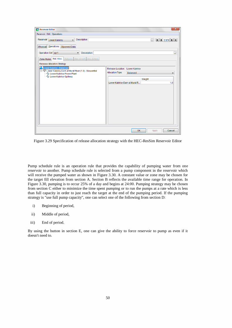
50
Figure 3.29 Specification of release allocation strategy with the HEC-ResSim Reservoir Editor
Pump schedule rule is an operation rule that provides the capability of pumping water from one
reservoir to another. Pump schedule rule is selected from a pump component in the reservoir which
will receive the pumped water as shown in Figure 3.30. A constant value or zone may be chosen for
the target fill elevation from section A. Section B reflects the available time range for operation. In
Figure 3.30, pumping is to occur 25% of a day and begins at 24:00. Pumping strategy may be chosen
from section C either to minimize the time spent pumping or to run the pumps at a rate which is less
than full capacity in order to just reach the target at the end of the pumping period. If the pumping
strategy is "use full pump capacity", one can select one of the following from section D:
i) Beginning of period,
ii) Middle of period,
iii) End of period.
By using the button in section E, one can give the ability to force reservoir to pump as even if it
doesn't need to.

51
Figure 3.30 Pump Rule Editor
HEC-ResSim offers several different ways of analyzing results. These include graphical plots of time-series variables, tables listing time-series of variables, and summary reports listing statistical measures
such as mean, maximum, minimum flow or water level. A number of pre-defined plots, tables and
reports are available. These pre-defined sets can be edited or new sets can be created. This offers the
possibility to produce outputs specifically focused on the problem to be analyzed. In addition, the
results can also be exported for post-processing in other software, such as for example MS Excel.
The real value of HEC-ResSim is to view a graphical display of the results on screen, as the zoom and
pan tools of HEC-ResSim offer an efficient, interactive way of analyzing time-series plots.
The following presentation of the results is intended to give an illustrative overview of the simulation
with HEC-ResSim. It is not a detailed presentation of all the results at each dam for each scenario.
Instead, the focus is on reporting results for any reservoir. Results for all dams and all scenarios and a
large number of variables are available in tabular forms in Chapter 4.
Examples for pre-defined plots include:
“Default plot” showing basic operation of the reservoir is shown in Figure 3.31.

52
Figure 3.31 Graphical display of "Default plot" function
“Power plot” showing energy generation is presented in Figure 3.32. This includes also a variable
showing the power capability, i.e. the power generation when all of the water is allocated to the
turbine. In the actual operation of the reservoir this power capability will not be reached due to
restrictions related to e.g. the guide curve, diversions and water requirements.

53
Figure 3.32 Graphical display of “Power plot” function
“Releases plot” showing all individual releases from the reservoir as shown in Figure 3.33. The
number of variables displayed here depends on the elements added to the specific reservoir.

54
Figure 3.33 Graphical display of “Releases plot” function

55
CHAPTER 4
3. SIMULATION ANALYSIS
4.1 Introduction
Upper Kaleköy Dam, the first facility at the upstream of Kaleköy reservoir system, is operated with
the inflows as shown in Figure 3.13. However, the downstream facilities are operated by adding the
intermediate flows to the power plant and spillway outflows of the upstream facility, from the
resulting flows. Usually upstream reservoirs are more important since they provide inflow for
downstream hydroplants.
The operation of four cascade reservoirs is simulated by considering ten different scenarios. The
model considers operation of the reservoirs with guide curves. In the operation scenarios for the dams,
power plant located at the toe of the dam has been simulated. Releases from the reservoirs include
turbined discharge, environmental flows, spillway losses, and evaporation losses. Diversion is
included to reflect water consumptions for irrigation.
Reservoir operation simulation primarily depends on the state of the reservoir at each time interval.
The general goal is to keep the reservoir at the top of the conservation pool. As the pool level moves
into flood, conservation, and inactive storage zones, the operation goals may change. The model was
performed on time-step from 6 hours to a day and simulates the coupled system of the four
hydropower plants. Main inputs of the simulation include:
i) Reservoir storage characteristics, as defined by the relationship volume-area-elevation.
ii) Evaporation from reservoir storage.
iii) Operation guide curve to determine release from reservoir storage.
iv) Tailwater rating-curve, which affects the hydraulic head as a function of runoff.
v) Environmental flow requirements.
vi) Broad consideration of hydraulic losses and turbine efficiency.
ix) Intra-daily turbine operation to allocate energy generation preferentially to peak hours as
opposed to off-peak hours.
x) Links between reservoirs, i.e. outflow from Upper Kaleköy is inflow to Lower Kaleköy,
outflow from Lower Kaleköy is inflow to Beyhan 1, and outflow from Beyhan 1 is inflow to
Beyhan 2.
xi) Intermediate inflow between reservoirs.
xii) Pump and turbine characteristics.
Reservoir system with many units may have various operational rules. An operational rule applied at
one reservoir will have consequences for other plants in the system. In this chapter, the various types
of operation rules and guide curves were investigated and the results of the scenarios are given in the
following sections.
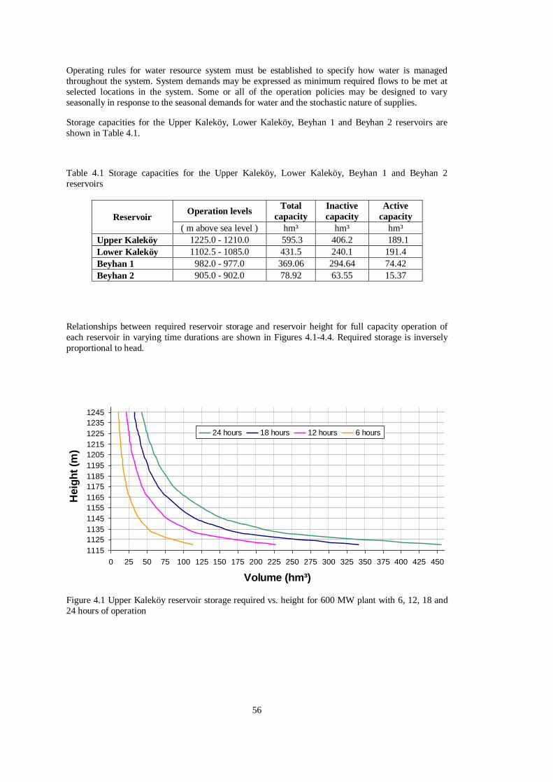
56
Operating rules for water resource system must be established to specify how water is managed
throughout the system. System demands may be expressed as minimum required flows to be met at
selected locations in the system. Some or all of the operation policies may be designed to vary
seasonally in response to the seasonal demands for water and the stochastic nature of supplies.
Storage capacities for the Upper Kaleköy, Lower Kaleköy, Beyhan 1 and Beyhan 2 reservoirs are
shown in Table 4.1.
Table 4.1 Storage capacities for the Upper Kaleköy, Lower Kaleköy, Beyhan 1 and Beyhan 2
reservoirs
Reservoir Operation levels
Total
capacity
Inactive
capacity
Active
capacity
( m above sea level ) hm³ hm³ hm³
Upper Kaleköy 1225.0 - 1210.0 595.3 406.2 189.1
Lower Kaleköy 1102.5 - 1085.0 431.5 240.1 191.4
Beyhan 1 982.0 - 977.0 369.06 294.64 74.42
Beyhan 2 905.0 - 902.0 78.92 63.55 15.37
Relationships between required reservoir storage and reservoir height for full capacity operation of
each reservoir in varying time durations are shown in Figures 4.1-4.4. Required storage is inversely
proportional to head.
1115
1125
1135
1145
1155
1165
1175
1185
1195
1205
1215
1225
1235
1245
0 25 50 75 100 125 150 175 200 225 250 275 300 325 350 375 400 425 450
Volume (hm³)
Heig
ht
(m)
24 hours 18 hours 12 hours 6 hours
Figure 4.1 Upper Kaleköy reservoir storage required vs. height for 600 MW plant with 6, 12, 18 and
24 hours of operation

57
1025
1035
1045
1055
1065
1075
1085
1095
1105
1115
1125
1135
0 25 50 75 100 125 150 175 200 225 250 275
Volume (hm³)
He
igh
t (m
)
24 hours 18 hours 12 hours 6 hours
Figure 4.2 Lower Kaleköy reservoir storage required vs. height for 450 MW plant with 6, 12, 18 and
24 hours of operation
920
930
940
950
960
970
980
990
1000
0 25 50 75 100 125 150 175 200
He
igh
t (m
)
Volume (hm³)
24 hours 18 hours 12 hours 6 hours
Figure 4.3 Beyhan 1 reservoir storage required vs. height for 550 MW plant with 6, 12, 18 and 24
hours of operation

58
890
900
910
920
930
940
950
960
0 20 40 60 80 100
Volume (hm³)
He
igh
t (m
)
24 hours 18 hours 12 hours 6 hours
Figure 4.4 Beyhan 2 reservoir storage required vs. height for 255 MW plant with 6, 12, 18 and 24
hours of operation
Unless otherwise mentioned, all scenarios have the same following definitions:
Hydrological scenario: Existing case.
Environmental scenario: Environmental flow requirements.
Four dams are under operation.
Simulation period: 40 years 1.10.2015 to 30.9.2055, daily time-steps.
Physical characteristics of the reservoirs mentioned in Chapter 3 were used.
Overload ratio is used by the program to determine the maximum energy where power plant
can produce in a time interval. The maximum production would then be a limit how much
excess energy could be generated during periods of surplus water. No overload ratio is
considered so it is taken as 1.
In Table 3.2, it was understood that environmental flow requirements are changing between wet and
dry seasons for all reservoirs. In all scenarios seasonal variation editor is used to specify releases.

59
Figure 4.5 Seasonal variation editor
For example, the minimum required release allowed at a downstream location is described as a
function of inflow at upstream location which is a function of internal variable. By using the seasonal variation option the simulations will obey the specified graph as shown in Figure 4.6 for Lower
Kaleköy reservoir. In this graph; it is seen that if the net inflows are higher than environmental flows,
the minimum release in dry seasons and wet seasons should be 20.15 m³/s and 40.31 m³/s
respectively.
Figure 4.6 Seasonal variation editor graph of Lower Kaleköy
In the scope of this study, ten scenarios have been investigated to utilize the hydraulic potential of
Murat River between the elevations of 870 m – 1225 m.

60
4.2 Scenario 1
Dam is operated continuously at maximum operation water level at all reservoirs. Operation studies were performed by using daily inflows in existing case.
Conservation zone comprises only environmental flow rule. HEC-ResSim tries to maintain the
reservoir water level specified in the conservation zone's top elevation. As an example, when the
Upper Kaleköy's reservoir water level exceeds 1225.0, the spillway is activated. In the inactive pool,
no releases are made. The only loss of water would come from evaporation.
Figure 4.7 shows a part of daily operating cycle. In this scenario, the plant is required to operate at
maximum operation level for 24 hours a day, seven days a week through all years. Not specifying
firm energy requirements provides an alternative strategy that will maximize the average annual
energy output.
The power duration curves shown in Figure 4.8-4.11 are based on all the time period of record. In
other words, it can be treated as an annual generation curve, describing the average annual output over
the period of record.
The average annual energy can be obtained by computing the area under the power output curve and
multiplying by the number of 8760 hrs.
where
P = generator output in kW
p = percent of time
As an example, the average annual energy for the Upper Kaleköy would be 1,398,955 kWh.
(4.1) dp Ppercent 100
hours 8760 (kWh)energy Annual
100
0
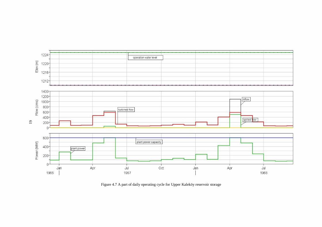
61
Figure 4.7 A part of daily operating cycle for Upper Kaleköy reservoir storage
61

62
Plant Factors are ratios indicating the portion of time that the plant is generating.
(4.2) capacity Installed x 24 x 365
energyyearly Averagefactor plant Annual
In Scenario 1 plant factors of Upper Kaleköy, Lower Kaleköy, Beyhan 1 and Beyhan 2 HEPPs are
0.27, 0.28, 0.26 and 0.25 respectively as shown in Table 4.2. In addition to this, the results of the
Scenario 1 are given in Table 4.2.
Table 4.2 Summary of results for Scenario 1
Name of
Facility
Annual net
inflow (hm³)
Annual flow
spill (m³/s)
Annual turbined
flow (m³/s)
Annual total
energy (GWh)
Plant
factors
Upper K. 5 254.3
407.0 4 846.3 1 399.0 0.27
Lower K.
Kaleköy
Kaleköy
Kaleköy
6 012.6
530.6 5 481.7 1 099.3 0.28
Beyhan 1 7 468.7
566.4 6 901.6 1 240.5 0.26
Beyhan 2 7 464.9
531.7 6 932.7 564.9 0.25
Total 26 200.5 2 035.7 24 162.3 4 303.7
0
100
200
300
400
500
600
700
% 0 % 10 % 20 % 30 % 40 % 50 % 60 % 70 % 80 % 90 % 100
Percentage of Time
Po
wer
Ou
tpu
t (M
W)
ss
0
200
400
600
800
1000
1200
1400
Daily
inflow
at U
pper
Kale
köy D
am
(m
³/s)Power output Net inflow
Figure 4.8 Power and net-inflow duration curve at Upper Kaleköy reservoir in Scenario 1

63
0
50
100
150
200
250
300
350
400
450
500
% 0 % 10 % 20 % 30 % 40 % 50 % 60 % 70 % 80 % 90 % 100
Percentage of Time
Pow
er O
utp
ut (M
W)
ss
0
200
400
600
800
1000
1200
1400
1600
Dai
ly i
nfl
ow
at
Lo
wer
Kal
ekö
y D
am,
m³/
s
Power output Net inflow
Figure 4.9 Power and net-inflow duration curve at Lower Kaleköy reservoir in Scenario 1
0
100
200
300
400
500
600
% 0 % 10 % 20 % 30 % 40 % 50 % 60 % 70 % 80 % 90 % 100
Percentage of Time
Pow
er O
utp
ut (M
W)
ss
0
200
400
600
800
1000
1200
1400
1600
1800
2000
Dail
y i
nfl
ow
at
Bey
han
1 D
am
, m
³/s
f
Power output Net inflow
Figure 4.10 Power and net-inflow duration curve at Beyhan 1 reservoir in Scenario 1

64
0
50
100
150
200
250
300
% 0 % 10 % 20 % 30 % 40 % 50 % 60 % 70 % 80 % 90 % 100
Percentage of Time
Pow
er O
utp
ut
(MW
) s
s
0
200
400
600
800
1000
1200
1400
1600
1800
2000
Dail
y i
nfl
ow
at
Bey
han
2 D
am
, m
³/s
f
Pow er output Net inflow
Figure 4.11 Power and net-inflow duration curve at Beyhan 2 reservoir in Scenario 1
4.3 Scenario 2
The aim of this scenario is to evaluate the change in power generation of Kaleköy reservoir system for
a 10% percent increase in the inflows. Inflows at all computation points were increased from the
Scenario 1 by 10 % for the Scenario 2.
On the local flow tab (Figure 4.12) of the junction editor, inflows were increased by a factor of 1.1 for each external flow entering the junction.
Higher inflow results in a increase in power generation of more than 7.8% at Kaleköy reservoir
system as shown in Table 4.3.
Table 4.3 Summary of results for Scenario 2
Name of
Facility
Annual
net
inflow
(hm³)
Annual flow
spill (m³/s)
Annual turbined
flow (m³/s)
Annual total
energy (GWh)
Upper K.
K.Kaleköy
5 780.5
554.6 5 224.8 1 507.7
Lower K. Kaleköy
Kaleköy
Kaleköy
Kaleköy
6 615.4
709.8 5 905.1 1 183.4 Beyhan 1 8 224.3
770.0 7 453.4 1 338.9
Beyhan 2 8 220.5 726.3 7 493.6 610.1
Total 28 840.7 2 760.7 26 076.9 4 640.1

65
Figure 4.12 %10 percent increase in local inflow at computation points
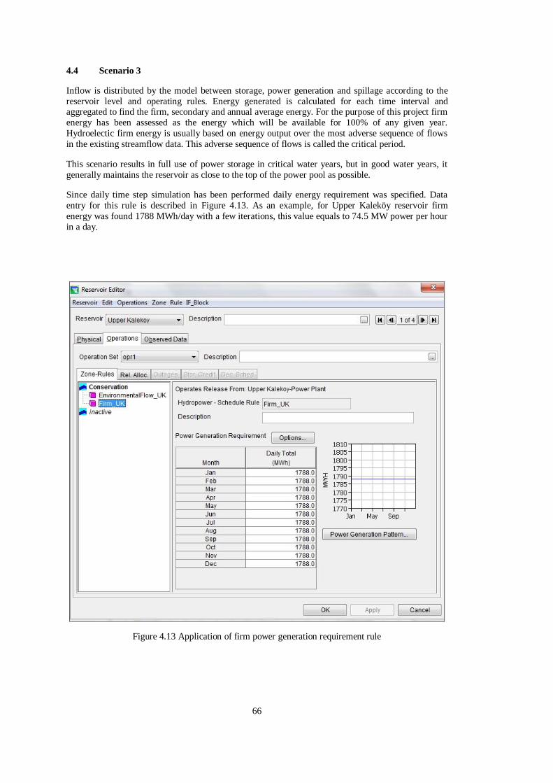
66
4.4 Scenario 3
Inflow is distributed by the model between storage, power generation and spillage according to the
reservoir level and operating rules. Energy generated is calculated for each time interval and aggregated to find the firm, secondary and annual average energy. For the purpose of this project firm
energy has been assessed as the energy which will be available for 100% of any given year.
Hydroelectic firm energy is usually based on energy output over the most adverse sequence of flows
in the existing streamflow data. This adverse sequence of flows is called the critical period.
This scenario results in full use of power storage in critical water years, but in good water years, it
generally maintains the reservoir as close to the top of the power pool as possible.
Since daily time step simulation has been performed daily energy requirement was specified. Data
entry for this rule is described in Figure 4.13. As an example, for Upper Kaleköy reservoir firm
energy was found 1788 MWh/day with a few iterations, this value equals to 74.5 MW power per hour
in a day.
Figure 4.13 Application of firm power generation requirement rule

67
Environmental flow and firm energy requirement rules limits the allowable release range of power
plants. In Figure 4.14, it is shown that because of the operation rules of Upper Kaleköy reservoir,
allowable range is limited between 71.25 - 582.00 m³/s.
Figure 4.14 Allowable turbined release range of Upper Kaleköy in Scenario 3
Note that the reservoir water levels are not identical to the conservation storage in the reservoir during
operation as shown in Figures 4.15-19, because of limitations imposed by inflows, environmental
flow and firm power requirements.
A review of the long-term flow records shows a period of markedly reduced flows in 2000 and 2001,
followed by high floods in the spring of 2002. These dry season years corresponds to 2050 and 2051
in simulation model. Therefore, the flow records from 2050 to 2051 are basis to determine the firm
power of the Upper Kaleköy plants during critical period as shown in Figure 4.16.
In Figures 4.16, the use of the term ‘critical period' begins at a point in time when the reservoir is full.
The end of the ‘critical period’ is defined as the point when the reservoir has refilled following the
drought period. The larger the amount of reservoir storage, the higher the firm yield or firm energy
output that can be sustained. Increasing the amount of reservoir storage also increases the length of
the critical period, sometimes even changing the critical period to a completely different sequence of
historical streamflows. Critical period may be a portion of a year, an entire year, or a period longer
than a year.

68
Same procedure is applied to all other three reservoirs. Since reservoirs have different volumes and
operation rules the time of critical period of each reservoir are not similar. In Figure 4.17, critical
period of Lower Kaleköy reservoir is summer of year 2024. In addition to this, critical period of
Beyhan 1 reservoir is summer of year 2034 as shown in Figure 4.18.
The procedure to find out the firm power capacity of each reservoir is simple. If the project fails to
use all of the storage, the preliminary energy estimate understates the project’s firm capability. The
monthly energy requirements were increased and the sequential routing was performed again in an
effort to fully use the storage.
If the project is drafted below the bottom of the power pool, the preliminary power requirement
estimate was too high. An adjustment was made similar to that described for the previous situation.
In either case, one or more additional iterations were made before the regulation exactly utilizes the
power storage and the reservoir fully refills. Once a satisfactory regulation obtained, the projects firm
energy output has been determined.

69
Figure 4.15 40 years time series simulation period operating cycle for Upper Kaleköy Dam and HEPP in Scenario 3
69

70
Figure 4.16 Critical period and critical drawdown period for Upper Kaleköy Dam and HEPP in Scenario 3
70

71
Figure 4.17 40 years time series simulation period operating cycle for Lower Kaleköy Dam and HEPP in Scenario 3
71

72
Figure 4.18 40 years time series simulation period operating cycle for Beyhan 1 Dam and HEPP in Scenario 3
72

73
Figure 4.19 40 years time series simulation period operating cycle for Beyhan 2 Dam and HEPP in Scenario 3
73

74
Energy generated in excess of a project or system’s firm energy output is defined as secondary
energy. Thus, it is produced in years outside of the critical period and is often concentrated primarily
in the high runoff season of those years. Secondary and firm energy generated at each power plant is
shown in Figure 4.20-23. Yellow region presents secondary energy and green region presents the firm
energy.
Secondary energy produced in years of higher inflow has to be maximised. This is achieved by
keeping the heads as high as possible and reducing energy losses by keeping spillway operation to a
minimum. The firm and secondary energy production values obtained for Upper Kaleköy, Lower Kaleköy, Beyhan 1 and Beyhan 2 dams on the basis of Scenario 3 are shown in Table 4.4.
Table 4.4 Summary of results for Scenario 3
Name of
Facility
Annual
net -
inflow
(hm³)
Annual
flow spill
(m³/s)
Annual
turbined
flow
(m³/s)
Firm
power
(MW)
Annual
firm
energy
(GWh)
Annual
secondary
energy
(GWh)
Annual
total
energy
(GWh)
Upper Kal. 5254.5
407.0 4848.4 74.5 653.1 735.8 1388.9
Lower Kal.
Kaleköy
Kaleköy
Kaleköy
6014.8 530.6 5485.3 58.0 508.4 583.0 1091.4
Beyhan 1 7472.6 566.4 6906.4 55.5 486.5 751.8 1238.3
Beyhan 2 7469.7 531.7 6937.6 25.0 219.6 345.7 565.3
Total 26211.6 2035.7 24177.7 213.0 1867.6 2416.3 4283.9
In Scenario 3 plant factors of Upper Kaleköy, Lower Kaleköy, Beyhan 1 and Beyhan 2 HEPPs are
0.26, 0.28, 0.26 and 0.25 respectively.

75
0
100
200
300
400
500
600
700
% 0
% 3
% 6
% 8
% 1
1
% 1
4
% 1
7
% 2
0
% 2
3
% 2
5
% 2
8
% 3
1
% 3
4
% 3
7
% 3
9
% 4
2
% 4
5
% 4
8
% 5
1
% 5
4
% 5
6
% 5
9
% 6
2
% 6
5
% 6
8
% 7
1
% 7
3
% 7
6
% 7
9
% 8
2
% 8
5
% 8
7
% 9
0
% 9
3
% 9
6
% 9
9
Percentage of time
Po
we
r O
utp
ut
(MW
)
0
200
400
600
800
1000
1200
1400
Da
ily
in
flo
w a
t U
pp
er
Ka
lek
öy
Da
m,
m³/
s
secondary energy
firm energy
net inflow
Figure 4.20 Power and net-inflow duration curve at Upper Kaleköy reservoir in Scenario 3
0
50
100
150
200
250
300
350
400
450
500
% 0
% 4
% 7
% 1
1
% 1
4
% 1
8
% 2
1
% 2
5
% 2
8
% 3
2
% 3
5
% 3
9
% 4
2
% 4
6
% 5
0
% 5
3
% 5
7
% 6
0
% 6
4
% 6
7
% 7
1
% 7
4
% 7
8
% 8
1
% 8
5
% 8
8
% 9
2
% 9
6
% 9
9
Percentage of time
Po
we
r O
utp
ut
(MW
)
0
200
400
600
800
1000
1200
1400
1600
Da
ily
in
flo
w a
t L
ow
er
Ka
lek
öy
Da
m,
m³/
s
secondary energy
firm energy
net inflow
Figure 4.21 Power and net-inflow duration curve at Lower Kaleköy reservoir in Scenario 3

76
0
100
200
300
400
500
600
% 0
% 4
% 7
% 1
1
% 1
4
% 1
8
% 2
1
% 2
5
% 2
8
% 3
2
% 3
6
% 3
9
% 4
3
% 4
6
% 5
0
% 5
3
% 5
7
% 6
0
% 6
4
% 6
8
% 7
1
% 7
5
% 7
8
% 8
2
% 8
5
% 8
9
% 9
2
% 9
6
% 9
9
Percentage of time
Po
we
r O
utp
ut
(MW
)
0
200
400
600
800
1000
1200
1400
1600
1800
2000
Daily in
flo
w a
t B
eyh
an
1 D
am
, m
³/s
secondary energyfirm energynet inflow
Figure 4.22 Power and net-inflow duration curve at Beyhan 1 reservoir in Scenario 3
0
50
100
150
200
250
300
% 0
% 3
% 7
% 1
0
% 1
4
% 1
7
% 2
1
% 2
4
% 2
8
% 3
1
% 3
5
% 3
8
% 4
2
% 4
5
% 4
9
% 5
2
% 5
6
% 5
9
% 6
3
% 6
6
% 7
0
% 7
3
% 7
7
% 8
0
% 8
4
% 8
7
% 9
1
% 9
4
% 9
8
Percentage of time
Po
we
r O
utp
ut
(MW
)
0
200
400
600
800
1000
1200
1400
1600
1800
2000
Da
ily
in
flo
w a
t B
ey
ha
n 2
Da
m,
m³/
s
secondary energy
firm energy
net inflow
Figure 4.23 Power and net-inflow duration curve at Beyhan 2 reservoir in Scenario 3

77
4.5 Scenario 4
The model is designed to compare power releases to meet firm energy requirements between existing
case (Scenario 3) and full development case. Since the inflow decreases in full development case, the firm energy generation decreases. The impacts of low inflow, result in considerable deviation on the
energy generation and operation water level.
The useful storage volume of the Upper, Lower Kaleköy and Beyhan 1 has provided considerable
hold-over storage capacity for inter-annual regulation, in other words a part of the flow in wet years
were stored in order to permit additional releases in subsequent dry years.
Table 4.5 lists the firm and secondary energy generation for the design scenario 4. It is shown that
there is a 20% decreases in total firm power and 16% decrease in total generated energy.
Table 4.5 Summary of results for Scenario 4
Name of
Facility
Annual
net -
inflow
(hm³)
Annual
flow spill
(m³/s)
Annual
turbined
flow
(m³/s)
Firm
power
(MW)
Annual
firm
energy
(GWh)
Annual
secondary
energy
(GWh)
Annual
total
energy
(GWh)
Upper Kal.
K
4106.2 170.7 3939.0 56.0 490.9 632.2 1123.1
Lower Kal.
Kaleköy
Kaleköy
Kaleköy
4868.7 261.4 4608.7 47.0 412.0 506.2 918.2
Beyhan 1 6326.6 318.8 6008.4 46.0 403.2 675.6 1078.8
Beyhan 2 6323.8 297.4 6026.2 20.8 182.3 309.7 492.0
Total 21 625.3 1 048.3 20 582.3 169.8 1 488.4 2 123.7 3 612.1
In Scenario 4 plant factors of Upper Kaleköy, Lower Kaleköy, Beyhan 1 and Beyhan 2 HEPPs
decreases to 0.21, 0.23, 0.22 and 0.22 respectively.
4.6 Scenario 5
Full development case time series were used in Scenario 5. In addition to this, all inputs and variables
are the same with Scenario 4 except that Lower Kaleköy's minimum operation level has been lowered
from 1085.0 to 1065.0 as shown in Figure 4.24. The reason is that in Feasibility Report (Temelsu
International Engineering Services Inc., 2011) sediment volume is at 1048.0 m however the intake level was chosen as 1069.0 m. Now it is considered to evaluate the effect of the increase in
conservation volume on power generation.

78
Figure 4.24 Revised storage zone at Lower Kaleköy reservoir in Scenario 5
With this assumption Table 4.6 lists the firm and secondary energy generation for the design Scenario
5.
Table 4.6 Summary of results for Scenario 5
Name of
Facility
Annual
net -
inflow
(hm³)
Annual
flow spill
(m³/s)
Annual
turbined
flow
(m³/s)
Firm
power
(MW)
Annual
firm
energy
(GWh)
Annual
secondary
energy
(GWh)
Annual
total
energy
(GWh)
Upper Kal.
K
4106.2 170.7 3939.0 56.0 490.9 632.2 1123.1
Lower Kal.
Kaleköy
Kaleköy
Kaleköy
4868.7 261.4 4609.1 48.1 421.6 489.3 910.9
Beyhan 1 6327.1 318.8 6009.0 47.4 415.5 663.5 1079.0
Beyhan 2 6324.4 297.4 6026.8 21.4 187.6 304.5 492.1
Total 21 626.4 1 048.3 20 583.9 172.9 1 515.6 2 089.5 3 605.1
In Scenario 5, plant factors of Upper Kaleköy, Lower Kaleköy, Beyhan 1 and Beyhan 2 HEPPs are 0.21, 0.23, 0.22 and 0.22 respectively.

79
4.7 Scenario 6
The model is designed to compare firm energy and total energy generation between Scenario 4 and
Scenario 6 at full development case. In Scenario 6, to determine the release from the reservoir in order to increase firm energy, some adjustments are made by iterations on the guide curve. Without any
other operational constraints, the decision logic will attempt to get to and keep the reservoir at the
guide curve, within maximum outlet capacity and physical rate of change constraints.
The coordinates of the points of the operation guide curves are specified by parameters, which are
subject to iterations. It is obvious that it is not required to iterate all coordinates of the points. For
example, it is obvious that the reservoir should be full after the snowmelt period. Similarly, to reduce
spillway losses the reservoir should be at a lower operation level before the onset of the snowmelt
runoff peak in spring.
Figure 4.25 shows a common operation guide curve for Kaleköy reservoir system. Usage of more
points on the operation guide curve is not desirable because of only insignificant increase in revenue
generation and the problem becomes considerably more complex.
Figure 4.25 A general example of guide curve for Kaleköy reservoir system
In Scenario 6, many iterations were made to increase the firm energy capacity of Kaleköy reservoir
system. In Figure 4.26, guide curves for related reservoirs are shown. In Figures 4.27-28 all simulation period is illustrated as an example for Lower Kaleköy reservoir.

80
Figure 4.26 Operation guide curves for Kaleköy reservoir system
Increase in firm energy does not mean increase in total annual energy or increase in benefit this
subject is discussed in Chapter 5. The results of Scenario 6 is summarized in Table 4.7.
Table 4.7 Summary of results for Scenario 6
Name of
Facility
Annual
net -
inflow
(hm³)
Annual
flow spill
(m³/s)
Annual
turbined
flow
(m³/s)
Firm
power
(MW)
Annual
firm
energy
(GWh)
Annual
secondary
energy
(GWh)
Annual
total
energy
(GWh)
Upper Kal.
K4106.2 149.7 3960.2 56.0 490.9 573.6 1064.5
Lower Kal.
Kaleköy
Kaleköy
Kaleköy
4868.9 209.9 4658.8 49.8 436.6 429.8 866.4
Beyhan 1 6325.6 262.2 6063.2 50.3 440.9 618.9 1059.8
Beyhan 2 6321.8 243.6 6077.8 22.8 199.9 297.0 496.9
Total 21 622.5 865.4 20 760 178.9 1 568.3 1 919.3 3 487.6
In Scenario 6, plant factors of Upper Kaleköy, Lower Kaleköy, Beyhan 1 and Beyhan 2 HEPPs are
0.20, 0.22, 0.22 and 0.22 respectively.

81
Figure 4.27 40 years time series simulation period operating cycle for Lower Kaleköy Dam and HEPP in Scenario 6
81

82
Figure 4.28 A closer look to the power plot for the critical period operating cycle for Lower Kaleköy Dam and HEPP in Scenario 6
82
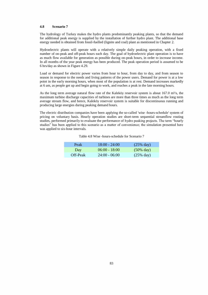
83
4.8 Scenario 7
The hydrology of Turkey makes the hydro plants predominantly peaking plants, so that the demand
for additional peak energy is supplied by the installation of further hydro plant. The additional base energy needed is obtained from fossil-fuelled (lignite and coal) plant as mentioned in Chapter 2.
Hydroelectric plants will operate with a relatively simple daily peaking operation, with a fixed
number of on-peak and off-peak hours each day. The goal of hydroelectric plant operation is to have
as much flow available for generation as possible during on-peak hours, in order to increase income.
In all months of the year peak energy has been produced. The peak operation period is assumed to be
6 hrs/day as shown in Figure 4.29.
Load or demand for electric power varies from hour to hour, from day to day, and from season to
season in response to the needs and living patterns of the power users. Demand for power is at a low
point in the early morning hours, when most of the population is at rest. Demand increases markedly
at 6 am, as people get up and begin going to work, and reaches a peak in the late morning hours.
As the long term average natural flow rate of the Kaleköy reservoir system is about 167.0 m³/s, the
maximum turbine discharge capacities of turbines are more than three times as much as the long term average stream flow, and hence, Kaleköy reservoir system is suitable for discontinuous running and
producing large energies during peaking demand hours.
The electric distribution companies have been applying the so-called 'wise -hours-schedule' system of
pricing on voluntary basis. Hourly operation studies are short-term sequential streamflow routing
studies, performed primarily to evaluate the performance of hydro peaking projects. The term “hourly
studies” has been applied to this scenario as a matter of convenience; the simulation presented here
was applied to six-hour intervals.
Table 4.8 Wise -hours-schedule for Scenario 7
Peak 18:00 - 24:00 (25% day)
Day 06:00 - 18:00 (50% day)
Off-Peak 24:00 - 06:00 (25% day)

84
Figure 4.29 Peak power generation operation cycle for Lower Kaleköy Dam and HEPP in Scenario 7
84

85
A number of factors influence the amount of peaking capacity of Kaleköy reservoir system at given
installed capacities and storage volumes:
i) average reservoir's inflows,
ii) time distribution of reservoir inflow,
iii) required generating pattern,
iv) required minimum discharge, v) reservoir elevation at start of weekly operating cycle,
vi) downstream discharge.
Table 4.9 Summary of results for Scenario 7
Name of
Facility
Production (GWh/year)
18-24 (T2) 06-18 (T1) 24-06 (T3) Total
Upper Kaleköy 798.76 379.30 150.95 1 329.01
Lower Kaleköy 608.25 283.72 118.93 1 010.90
Beyhan 1 712.72 355.98 144.10 1 212.80
Beyhan 2 323.46 160.82 64.29 548.57
The power duration curves shown in Figures 4.30-4.33 illustrate what percentage of the time peak
power operation occurs in Kaleköy reservoir system.
0
100
200
300
400
500
600
700
% 0 % 10 % 20 % 30 % 40 % 50 % 60 % 70 % 80 % 90 % 100
Percentage of Time
Po
wer
Ou
tpu
t (M
W)
ss
0
200
400
600
800
1000
1200
1400
Dail
y i
nfl
ow
at
Up
per
Kale
kö
y D
am
(m
³/s)
s
Power output Inflow
Figure 4.30 Power and net-inflow duration curve at Upper Kaleköy reservoir in Scenario 7

86
0
50
100
150
200
250
300
350
400
450
500
% 0 % 10 % 20 % 30 % 40 % 50 % 60 % 70 % 80 % 90 % 100
Percentage of Time
Pow
er O
utp
ut
(MW
) s
s
0
200
400
600
800
1000
1200
1400
1600
Dail
y i
nfl
ow
at
Low
er K
ale
köy D
am
(m
³/s)
s
Power output Inflow
Figure 4.31 Power and net-inflow duration curve at Lower Kaleköy reservoir in Scenario 7
0
100
200
300
400
500
600
% 0 % 10 % 20 % 30 % 40 % 50 % 60 % 70 % 80 % 90 % 100
Percentage of Time
Pow
er O
utp
ut
(MW
) s
s
0
200
400
600
800
1000
1200
1400
1600
1800
2000
Dail
y i
nfl
ow
at
Bey
han
1 D
am
(m
³/s)
s
Power output Inflow
Figure 4.32 Power and net-inflow duration curve at Beyhan 1 reservoir in Scenario 7
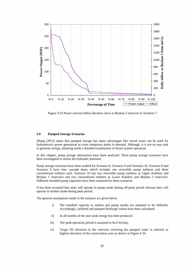
87
0
50
100
150
200
250
300
% 0 % 10 % 20 % 30 % 40 % 50 % 60 % 70 % 80 % 90 % 100
Percentage of Time
Po
wer
Ou
tpu
t (M
W)
ss
0
200
400
600
800
1000
1200
1400
1600
1800
2000
Da
ily
in
flo
w a
t B
eyh
an
2 D
am
(m
³/s)
s
Power output Inflow
Figure 4.33 Power and net-inflow duration curve at Beyhan 2 reservoir in Scenario 7
4.9 Pumped Storage Scenarios
Zhang (2012) states that pumped storage has many advantages like stored water can be used for
hydroelectric power generation to cover temporary peaks in demand. Although, it is not an easy task
to generate energy, planning needs a detailed examination of future system operation.
In this chapter, pump storage alternatives have been analyzed. Three pump storage scenarios have been investigated to utilize the hydraulic potential.
Pump storage scenarios have been studied for Scenario 8, Scenario 9 and Scenario 10. Scenario 8 and
Scenario 9 have four cascade dams which includes one reversible pump turbines and three
conventional turbines each. Scenario 10 has two reversible pump turbines as Upper Kaleköy and
Beyhan 1 reservoirs and two conventional turbines as Lower Kaleköy and Beyhan 2 reservoirs.
Different installed pump capacities have been analyzed for these scenarios.
It has been accepted that units will operate in pump mode during off-peak period whereas they will
operate in turbine mode during peak period.
The general assumptions made in the analyses are given below.
i) The installed capacity in turbine and pump modes are assumed to be different.
Accordingly, turbined and pumped discharge values have been calculated.
ii) In all months of the year peak energy has been produced.
iii) The peak operation period is assumed to be 6 hrs/day.
iv) Target fill elevation in the reservoir receiving the pumped water is selected as
highest elevation of the conservation zone as shown in Figure 4.34.

88
v) Full pump capacity strategy is selected. It will minimize the time spent for pumping.
As a result of this, sometimes there are more time available in the pumping period
than is needed to get the reservoir pool back to its target elevation.
vi) Minimum pumping option is not selected, since there is no need to force the
reservoir to pump, even if it doesn’t need to.
vii) A fixed hour range is specified for daily pumping period as shown in Figure 4.34.
The maximum duration of pumping is taken as 6 hrs/day.
Figure 4.34 Reservoir editor tab to define the physical characteristics of pump
Daily pumping period is selected from midnight to 6:00 am. In additon to this, since water is pumped back to the upper reservoir there is no need to turbine environmental flow between off-peak hours
(24:00-06:00). Hour of day multiplier operation allows us to specify a factor that will be applied to the
release specified by environmental flow rule as shown in Figure 4.35. Since environmental release
rule is not required during pumping period, it is set the multiplier for off-peak hours to 0.0 and all
other to 1.0.

89
Figure 4.35 Hour of day multiplier with values of 0.0 and 1.0 specified for a portion of day
Since there are many types of machines appropriate for pumped-storage applications, the type is
selected by the available head. Single-stage reversible Francis turbines are best choice between 50 to
800 m range. If the head is above 800 m, multi stage units or seperate pump and turbines should be
considered (Voith, 2009). In addition to this, in near future with improvement in technology single-stage Francis units may be used for greater than 800 m. Figure 4.36 illustrates the performance range
for pump-turbines.
In pumped storage Scenario 8 and Scenario 10, Upper Kaleköy reservoir has a reversible turbine
which has a 550 MW installed capacity in pump mode 600 MW installed capacity in turbine mode. In
addition to this, Beyhan 1 reservoir has a reversible turbine which has a 500 MW installed capacity in
pump mode 550 MW installed capacity in turbine mode in Scenario 9 and Scenario 10. Lower
Kaleköy and Beyhan 1 reservoirs have the same installed capacities in all scenarios as 450 MW and
255 MW respectively.

90
Figure 4.36 Performance range for pump-turbines (Voith, 2009)
Regardless of pumping strategy selection, if the target cannot be reached in the pumping period, the
pumps will be operated at full capacity over the entire pumping period in order to get as close to the
target as possible.
Same head losses presented in Chapter 3.5 in turbine mode are used in pump mode too. Hydraulic
losses for Upper Kaleköy and Beyhan 1 pump-turbines are 2.5 and 2.0 m, respectively.
4.9.1 Scenario 8
In this scenario, Upper Kaleköy Dam at the upstream will be upper reservoir whereas Lower Kaleköy
Dam at the downstream will be the lower reservoir in the system as shown in Figure 4.37. The power
plant of the upper reservoir will be equipped with reversible pump-turbines. In pump mode the water
from Lower Kaleköy reservoir will flow to Upper Kaleköy reservoir during off-peak hours between
24:00-06:00. In turbine mode the water from Upper Kaleköy reservoir will flow to Lower Kaleköy
reservoir between 06:00-24:00 hours. Operation cycle is shown in Figure 4.38 for 40 years long time
series.

91
Maximum Operation Water Level = 1225.0
Minimum Operation Water Level = 1210.0
UPPER KALEKÖY AND HEPP
( UPPER RESERVOIR )
Reversible
Pump-turbine
LOWER KALEKÖY AND HEPP
Conventional
Turbine
Maximum O.W.L. = 1102.5
1090.0
Minimum O.W.L. = 1085.0
Allowable Pump
Operation Head
( LOWER RESERVOIR )Not to scale.
Figure 4.37 Visual presentation of Scenario 8
Figure 4.38 40 years long time series simulation period operating cycle for Upper Kaleköy Dam and HEPP in Scenario 8
91

92
In Hec-ResSim it is not possible to get directly the consumed energy during pump mode. By simple
calculations it is easy to find out pumped energy at each time step. For example, on the first day of
February in 2016 at Upper Kaleköy, net head (124.67 m) is assumed as hydraulic loss (2.5 m) plus
gross head (122.17 m) in Table 4.10. Then energy for pumping is calculated (3226.77 MWh) by
multiplying net head (124.67) with maximum pump discharge (395.75 m³/s) for six hours and finally
divide by pump efficiency (0.9).
Table 4.10 Calculation methodology of consumed pump energy
Time
simulation results calculated
Upper
Kaleköy
Lower
Kaleköy Pumping
Gross
Pump
Net
Pump
Consumed
Pump
Pool
Elevation
Pool
Elevation
Duration Head Head Energy
(m) (m) (hr) (m) (m) MWh
29Jan2016
24:00 1224.51 1102.5 0.00 122.26 124.76 435.91
30Jan2016
06:00 1225.00 1102.5 0.81
30Jan2016
24:00 1224.51 1102.5 0.00 122.26 124.76 435.91
31Jan2016
06:00 1225.00 1102.5 0.81
31Jan2016
24:00 1224.51 1102.5 0.00 122.26 124.76 1862.04
01Feb2016
06:00 1225.00 1102.5 3.46
01Feb2016
24:00 1224.25 1102.4 0.00 122.17 124.67 3226.77
02Feb2016
06:00 1224.99 1102.5 6.00
02Feb2016
24:00 1224.25 1102.13 0.00 122.31 124.81 3230.26
The results of the analyses performed considering the given assumptions are summarized in Table
4.11.
Table 4.11 Summary of results for Scenario 8
Sometimes, natural flows in combination with available pondage may be sufficient to support the
plants peaking capacity. On the contrary, pumping water to upstream reservoir may not be possible
due to the insufficient pump operation head as shown in Figure 4.39. During low flow periods,
however, a portion of the peaking discharge would be pumped back at night, to insure that sufficient
water is available to meet peaking requirements on subsequent days.
Name of
Facility
Production (GWh/year)
Pumping
24-06
18-24
(T2)
06-18
(T1)
24-06
(T3) Total
Upper Kaleköy - 781.0 1276.0 531.0 117.8 1143.8
Lower Kaleköy 612.3 350.1 96.2 1058.6
Beyhan 1 681.2 397.8 132.0 1211.0
Beyhan 2 313.8 180.4 59.4 553.6

93
Figure 4.39 Peak operation of Scenario 8
93
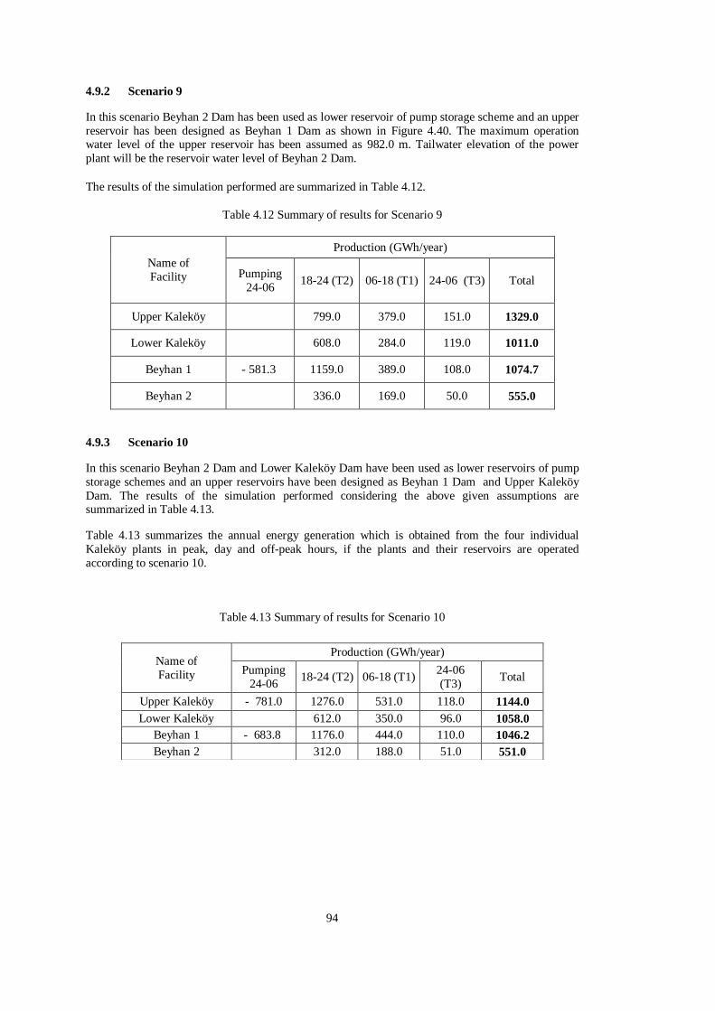
94
4.9.2 Scenario 9
In this scenario Beyhan 2 Dam has been used as lower reservoir of pump storage scheme and an upper
reservoir has been designed as Beyhan 1 Dam as shown in Figure 4.40. The maximum operation water level of the upper reservoir has been assumed as 982.0 m. Tailwater elevation of the power
plant will be the reservoir water level of Beyhan 2 Dam.
The results of the simulation performed are summarized in Table 4.12.
Table 4.12 Summary of results for Scenario 9
Name of
Facility
Production (GWh/year)
Pumping
24-06 18-24 (T2) 06-18 (T1) 24-06 (T3) Total
Upper Kaleköy 799.0 379.0 151.0 1329.0
Lower Kaleköy 608.0 284.0 119.0 1011.0
Beyhan 1 - 581.3 1159.0 389.0 108.0 1074.7
Beyhan 2 336.0 169.0 50.0 555.0
4.9.3 Scenario 10
In this scenario Beyhan 2 Dam and Lower Kaleköy Dam have been used as lower reservoirs of pump
storage schemes and an upper reservoirs have been designed as Beyhan 1 Dam and Upper Kaleköy
Dam. The results of the simulation performed considering the above given assumptions are summarized in Table 4.13.
Table 4.13 summarizes the annual energy generation which is obtained from the four individual
Kaleköy plants in peak, day and off-peak hours, if the plants and their reservoirs are operated
according to scenario 10.
Table 4.13 Summary of results for Scenario 10
Name of
Facility
Production (GWh/year)
Pumping
24-06 18-24 (T2) 06-18 (T1)
24-06
(T3) Total
Upper Kaleköy - 781.0 1276.0 531.0 118.0 1144.0
Lower Kaleköy 612.0 350.0 96.0 1058.0
Beyhan 1 - 683.8 1176.0 444.0 110.0 1046.2
Beyhan 2 312.0 188.0 51.0 551.0

95
Maximum Operation Water Level = 982
Minimum Operation Water Level = 977
BEYHAN 1 DAM AND HEPP
( UPPER RESERVOIR )
Reversible
Pump-turbine
BEYHAN 2 DAM AND HEPP
Conventional
Turbine
Maximum O .W.L. = 905
Minimum O .W.L. = 902
Allowable Pump
Operation Head
( LOWER RESERVOIR )Not to scale.
Figure 4.40 Visual presentation of Scenario 9
95

96

97
CHAPTER 5
4. FINANCIAL ANALYSIS
5.1 Introduction
The purpose of this chapter is highlighting the effectiveness of the analyzed scenarios for the
operation period of 50 years. Based on the following economic scenario ratios, there will be necessary
information for future investments.
In addition to the reservoir model, also financial analyses are presented for the comparison of the
scenarios. In Figure 5.1 general structure of the financial model is shown.
Figure 5.1 General structure of the financial model
5.2 Cost of Facilities
Costs of facilities proposed for Kaleköy reservoir system have been based on quantity estimation
obtained from Feasibility Report (Temelsu International Engineering Services Inc., 2011).
Construction costs have been calculated for Scenarios 1 to 7 in Table 5.3, for Scenario 8 in Table 5.6,
for Scenario 9 in Table 5.9, and for Scenario 10 in Table 5.12. In pumped storage scenarios (Scenario
8, 9, 10), the difference between unit price of electromechanical equipment for conventional turbine
and pump-turbine has been taken as 100 USD/kW.
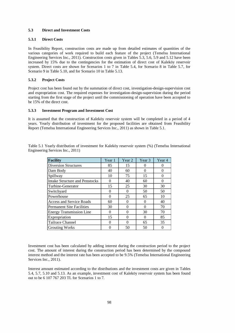
98
5.3 Direct and Investment Costs
5.3.1 Direct Costs
In Feasibility Report, construction costs are made up from detailed estimates of quantities of the
various categories of work required to build each feature of the project (Temelsu International Engineering Services Inc., 2011). Construction costs given in Tables 5.3, 5.6, 5.9 and 5.12 have been
increased by 15% due to the contingencies for the estimation of direct cost of Kaleköy reservoir
system. Direct costs are shown for Scenarios 1 to 7 in Table 5.4, for Scenario 8 in Table 5.7, for
Scenario 9 in Table 5.10, and for Scenario 10 in Table 5.13.
5.3.2 Project Costs
Project cost has been found out by the summation of direct cost, investigation-design-supervision cost
and expropriation cost. The required expenses for investigation-design-supervision during the period
starting from the first stage of the project until the commissioning of operation have been accepted to
be 15% of the direct cost.
5.3.3 Investment Program and Investment Cost
It is assumed that the construction of Kaleköy reservoir system will be completed in a period of 4
years. Yearly distribution of investment for the proposed facilities are obtained from Feasibility
Report (Temelsu International Engineering Services Inc., 2011) as shown in Table 5.1.
Table 5.1 Yearly distribution of investment for Kaleköy reservoir system (%) (Temelsu International Engineering Services Inc., 2011)
Facility Year 1 Year 2 Year 3 Year 4
Diversion Structures 85 15 0 0
Dam Body 40 60 0 0
Spillway 10 75 15 0
Intake Structure and Penstocks 0 40 60 0
Turbine-Generator 15 25 30 30
Switchyard 0 0 50 50
Powerhouse 0 25 65 10
Access and Service Roads 60 0 0 40
Permanent Site Facilities 30 0 0 70
Energy Transmission Line 0 0 30 70
Expropriation 15 0 0 85
Tailrace Channel 0 0 65 35
Grouting Works 0 50 50 0
Investment cost has been calculated by adding interest during the construction period to the project cost. The amount of interest during the construction period has been determined by the compound
interest method and the interest rate has been accepted to be 9.5% (Temelsu International Engineering
Services Inc., 2011).
Interest amount estimated according to the distributions and the investment costs are given in Tables
5.4, 5.7, 5.10 and 5.13. As an example, investment cost of Kaleköy reservoir system has been found
out to be 6 107 767 203 TL for Scenarios 1 to 7.
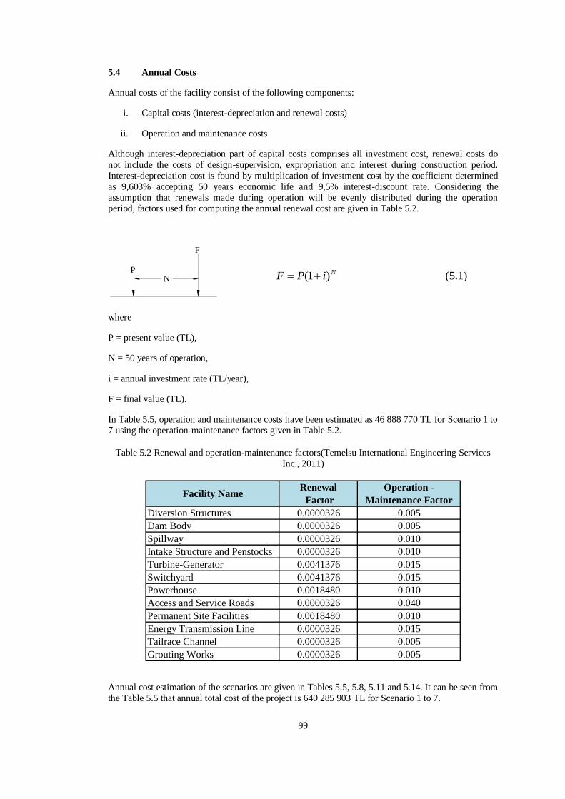
99
5.4 Annual Costs
Annual costs of the facility consist of the following components:
i. Capital costs (interest-depreciation and renewal costs)
ii. Operation and maintenance costs
Although interest-depreciation part of capital costs comprises all investment cost, renewal costs do
not include the costs of design-supervision, expropriation and interest during construction period.
Interest-depreciation cost is found by multiplication of investment cost by the coefficient determined
as 9,603% accepting 50 years economic life and 9,5% interest-discount rate. Considering the
assumption that renewals made during operation will be evenly distributed during the operation
period, factors used for computing the annual renewal cost are given in Table 5.2.
NP
F
where
P = present value (TL),
N = 50 years of operation,
i = annual investment rate (TL/year),
F = final value (TL).
In Table 5.5, operation and maintenance costs have been estimated as 46 888 770 TL for Scenario 1 to
7 using the operation-maintenance factors given in Table 5.2.
Table 5.2 Renewal and operation-maintenance factors(Temelsu International Engineering Services
Inc., 2011)
Diversion Structures 0.0000326 0.005
Dam Body 0.0000326 0.005
Spillway 0.0000326 0.010
Intake Structure and Penstocks 0.0000326 0.010
Turbine-Generator 0.0041376 0.015
Switchyard 0.0041376 0.015
Powerhouse 0.0018480 0.010
Access and Service Roads 0.0000326 0.040
Permanent Site Facilities 0.0018480 0.010
Energy Transmission Line 0.0000326 0.015
Tailrace Channel 0.0000326 0.005
Grouting Works 0.0000326 0.005
Renewal
Factor
Operation -
Maintenance FactorFacility Name
Annual cost estimation of the scenarios are given in Tables 5.5, 5.8, 5.11 and 5.14. It can be seen from
the Table 5.5 that annual total cost of the project is 640 285 903 TL for Scenario 1 to 7.
(5.1) )1( NiPF

100
Table 5.3 Construction costs for Scenario 1, 2, 3, 4, 5, 6 and 7
Upper Kaleköy Lower Kaleköy Beyhan 1 Beyhan 2 Construction Cost
Dam and HEPP Dam and HEPP Dam and HEPP Dam and HEPP (TL)
Diversion Structures 92 454 419 83 266 051 114 261 054 9 740 832 299 722 356
Dam Body 309 582 813 170 828 892 198 578 522 95 312 716 774 302 943
Spillway 87 574 319 82 995 205 95 272 977 190 229 564 456 072 065
Intake Structure and Penstocks 113 769 817 89 150 970 59 673 664 96 589 571 359 184 022
Turbine-Generator 387 000 000 338 625 000 378 400 000 191 887 500 1295 912 500
Switchyard 12 900 000 9 675 000 11 825 000 5 482 500 39 882 500
Powerhouse 64 500 000 48 375 000 59 125 000 27 412 500 199 412 500
Access and Service Roads 20 850 000 13 850 000 14 462 429 16 000 000 65 162 429
Permanent Site Facilities 778 750 778 750 772 880 772 880 3 103 260
Energy Transmission Line 32 775 000 40 470 000 44 000 000 26 790 000 144 035 000
Tailrace Channel 14 173 744 15 837 750 2 184 985 12 447 677 44 644 156
Grouting Works 7 999 713 6 893 745 7 668 432 17 004 254 39 566 144
Expropriation 27 300 000 19 900 000 31 500 000 3 300 000
3 720 999 875
Name of the Facility
10
0

101
Table 5.4 Calculation of investment costs for Scenario 1, 2, 3, 4, 5, 6 and 7
INVESTMENT Construction Cost Direct Cost Investigation-Design Investment Cost
Name of the Facility (TL) (TL) Supervision (TL) Year 1 Year 2 Year 3 Year 4 Total Year 1 Year 2 Year 3 Year 4 Total (TL)
Diversion Structures 299 722 356 344 680 709 51 702 106 336 925 393 59 457 422 0 0 396 382 816 125 970 322 15 143 015 0 0 141 113 338 537 496 153
Dam Body 774 302 943 890 448 384 133 567 258 409 606 257 614 409 385 0 0 1024 015 642 153 144 385 156 481 905 0 0 309 626 290 1333 641 932
Spillway 456 072 065 524 482 875 78 672 431 60 315 531 452 366 479 90 473 296 0 603 155 306 22 550 888 115 211 730 13 193 957 0 150 956 576 754 111 882
Intake Structure 359 184 022 413 061 625 61 959 244 0 190 008 348 285 012 521 0 475 020 869 0 48 392 601 41 564 120 0 89 956 721 564 977 591
Turbine-Generator 1295 912 500 1490 299 375 223 544 906 257 076 642 428 461 070 514 153 284 514 153 284 1713 844 281 96 116 316 109 123 340 74 980 316 23 868 269 304 088 242 2017 932 523
Switchyard 39 882 500 45 864 875 6 879 731 0 0 26 372 303 26 372 303 52 744 606 0 0 3 845 942 1 224 268 5 070 209 57 814 816
Powerhouse 199 412 500 229 324 375 34 398 656 0 65 930 758 171 419 970 26 372 303 263 723 031 0 16 791 688 24 998 622 1 224 268 43 014 577 306 737 609
Access and Service Roads 65 162 429 74 936 793 11 240 519 51 706 387 0 0 34 470 925 86 177 312 19 332 085 0 0 1 600 226 20 932 311 107 109 623
Permanent Site Facilities 3 103 260 3 568 749 535 312 1 231 218 0 0 2 872 843 4 104 061 460 330 0 0 133 364 593 695 4 697 756
Energy Transmission Line 144 035 000 165 640 250 24 846 038 0 0 57 145 886 133 340 401 190 486 288 0 0 8 333 734 6 189 992 14 523 726 205 010 013
Tailrace Channel 44 644 156 51 340 779 7 701 117 0 0 38 377 233 20 664 664 59 041 896 0 0 5 596 652 959 305 6 555 957 65 597 853
Grouting Works 39 566 144 45 501 066 6 825 160 0 26 163 113 26 163 113 0 52 326 225 0 6 663 397 3 815 435 0 10 478 832 62 805 058
Expropriation 0 0 12 300 000 0 0 69 700 000 82 000 000 4 598 748 0 0 3 235 647 7 834 395 89 834 395
3 720 999 875 4 279 149 856 641 872 478 1 129 161 429 1 836 796 576 1 209 117 607 827 946 723 5 003 022 335 422 173 074 467 807 677 176 328 779 38 435 338 1 104 744 868 6 107 767 203
Project Cost (TL) Interest During Construction (TL)
Table 5.5 Calculation of annual costs for Scenario 1, 2, 3, 4, 5, 6 and 7
COST Construction Cost Direct Cost Project Cost Interest Investment
Name of the Facility (TL) (TL) (TL) During Construction Cost (TL) Interest-Depreciation Renewal Operation-Maintenance Total
1 Diversion Structures 299 722 356 344 680 709 396 382 816 141 113 338 537 496 153 51 615 756 11 237 1 723 404 53 350 396
2 Dam Body 774 302 943 890 448 384 1024 015 642 309 626 290 1333 641 932 128 069 635 29 029 4 452 242 132 550 905
3 Spillway 456 072 065 524 482 875 603 155 306 150 956 576 754 111 882 72 417 364 17 098 5 244 829 77 679 291
4 Intake Structure and Penstocks 359 184 022 413 061 625 475 020 869 89 956 721 564 977 591 54 254 798 13 466 4 130 616 58 398 880
5 Turbine-Generator 1295 912 500 1490 299 375 1713 844 281 304 088 242 2017 932 523 193 782 060 6 166 263 22 354 491 222 302 813
6 Switchyard 39 882 500 45 864 875 52 744 606 5 070 209 57 814 816 5 551 957 189 771 687 973 6 429 700
7 Powerhouse 199 412 500 229 324 375 263 723 031 43 014 577 306 737 609 29 456 013 423 791 2 293 244 32 173 048
8 Access and Service Roads 65 162 429 74 936 793 86 177 312 20 932 311 107 109 623 10 285 737 2 443 2 997 472 13 285 652
9 Permanent Site Facilities 3 103 260 3 568 749 4 104 061 593 695 4 697 756 451 126 6 595 35 687 493 408
10 Energy Transmission Line 144 035 000 165 640 250 190 486 288 14 523 726 205 010 013 19 687 112 5 400 2 484 604 22 177 115
11 Tailrace Channel 44 644 156 51 340 779 59 041 896 6 555 957 65 597 853 6 299 362 1 674 256 704 6 557 739
12 Grouting Works 39 566 144 45 501 066 52 326 225 10 478 832 62 805 058 6 031 170 1 483 227 505 6 260 158
13 Expropriation 82 000 000 7 834 395 89 834 395 8 626 797 8 626 797
Total 3 720 999 875 4 279 149 856 5 003 022 335 1 104 744 868 6 107 767 203 586 528 884 6 868 249 46 888 770 640 285 903
Annual Costs (TL)
NP
F
10
1

102
Table 5.6 Construction costs for Scenario 8
Upper Kalekoy Lower Kalekoy Beyhan 1 Beyhan 2 Construction Cost
Dam and HEPP Dam and HEPP Dam and HEPP Dam and HEPP (TL)
Diversion Structures 92 454 419 83 266 051 114 261 054 9 740 832 299 722 356
Dam Body 309 582 813 170 828 892 198 578 522 95 312 716 774 302 943
Spillway 87 574 319 82 995 205 95 272 977 190 229 564 456 072 065
Intake Structure and Penstocks 113 769 817 89 150 970 59 673 664 96 589 571 359 184 022
Reversible-turbine and Generator 475 000 000 338 625 000 378 400 000 191 887 500 1383 912 500
Switchyard 12 900 000 9 675 000 11 825 000 5 482 500 39 882 500
Powerhouse 64 500 000 48 375 000 59 125 000 27 412 500 199 412 500
Access and Service Roads 20 850 000 13 850 000 14 462 429 16 000 000 65 162 429
Permanent Site Facilities 778 750 778 750 772 880 772 880 3 103 260
Energy Transmission Line 32 775 000 40 470 000 44 000 000 26 790 000 144 035 000
Tailrace Channel 14 173 744 15 837 750 2 184 985 12 447 677 44 644 156
Grouting Works 7 999 713 6 893 745 7 668 432 17 004 254 39 566 144
Expropriation 27 300 000 19 900 000 31 500 000 3 300 000
3 808 999 875
Installed Capacity to Upper Kalekoy 550.0 MW x 100.0 USD/kW = 55 000 000 USD
1 USD = 1.60 TL
= 88 000 000TL
Name of the Facility
Additional Reversible Pump-Turbine
10
2
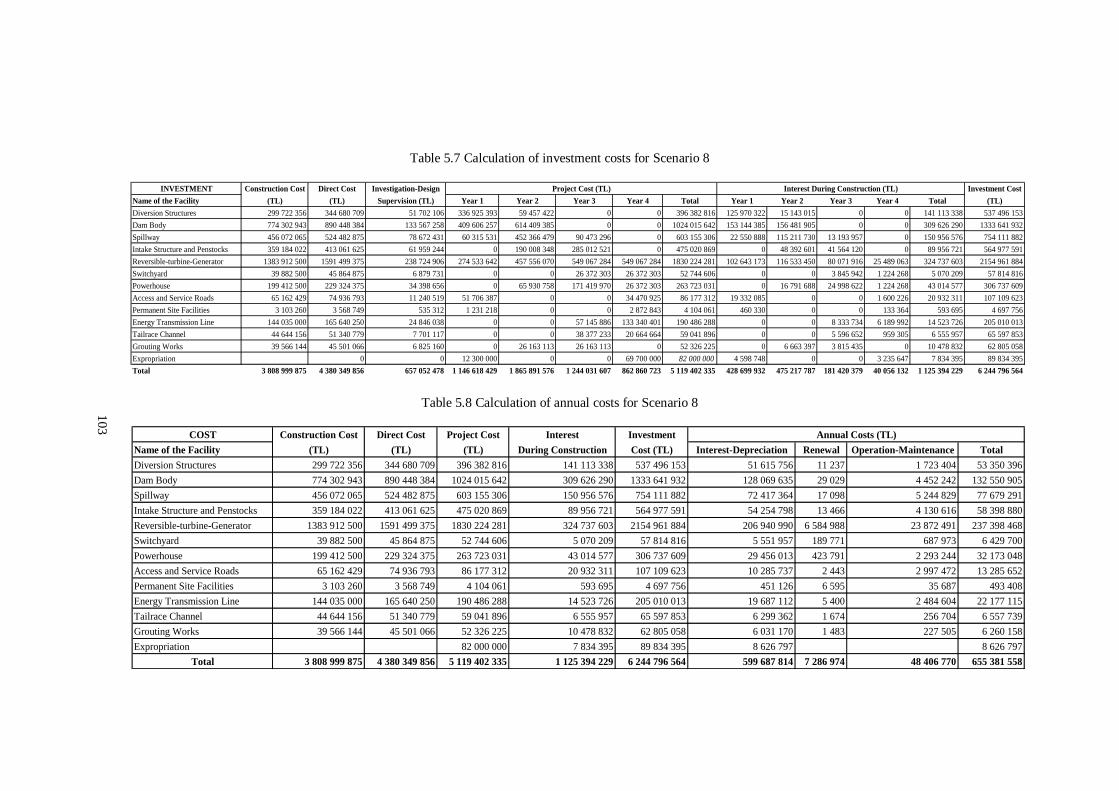
103
Table 5.7 Calculation of investment costs for Scenario 8
INVESTMENT Construction Cost Direct Cost Investigation-Design Investment Cost
Name of the Facility (TL) (TL) Supervision (TL) Year 1 Year 2 Year 3 Year 4 Total Year 1 Year 2 Year 3 Year 4 Total (TL)
Diversion Structures 299 722 356 344 680 709 51 702 106 336 925 393 59 457 422 0 0 396 382 816 125 970 322 15 143 015 0 0 141 113 338 537 496 153
Dam Body 774 302 943 890 448 384 133 567 258 409 606 257 614 409 385 0 0 1024 015 642 153 144 385 156 481 905 0 0 309 626 290 1333 641 932
Spillway 456 072 065 524 482 875 78 672 431 60 315 531 452 366 479 90 473 296 0 603 155 306 22 550 888 115 211 730 13 193 957 0 150 956 576 754 111 882
Intake Structure and Penstocks 359 184 022 413 061 625 61 959 244 0 190 008 348 285 012 521 0 475 020 869 0 48 392 601 41 564 120 0 89 956 721 564 977 591
Reversible-turbine-Generator 1383 912 500 1591 499 375 238 724 906 274 533 642 457 556 070 549 067 284 549 067 284 1830 224 281 102 643 173 116 533 450 80 071 916 25 489 063 324 737 603 2154 961 884
Switchyard 39 882 500 45 864 875 6 879 731 0 0 26 372 303 26 372 303 52 744 606 0 0 3 845 942 1 224 268 5 070 209 57 814 816
Powerhouse 199 412 500 229 324 375 34 398 656 0 65 930 758 171 419 970 26 372 303 263 723 031 0 16 791 688 24 998 622 1 224 268 43 014 577 306 737 609
Access and Service Roads 65 162 429 74 936 793 11 240 519 51 706 387 0 0 34 470 925 86 177 312 19 332 085 0 0 1 600 226 20 932 311 107 109 623
Permanent Site Facilities 3 103 260 3 568 749 535 312 1 231 218 0 0 2 872 843 4 104 061 460 330 0 0 133 364 593 695 4 697 756
Energy Transmission Line 144 035 000 165 640 250 24 846 038 0 0 57 145 886 133 340 401 190 486 288 0 0 8 333 734 6 189 992 14 523 726 205 010 013
Tailrace Channel 44 644 156 51 340 779 7 701 117 0 0 38 377 233 20 664 664 59 041 896 0 0 5 596 652 959 305 6 555 957 65 597 853
Grouting Works 39 566 144 45 501 066 6 825 160 0 26 163 113 26 163 113 0 52 326 225 0 6 663 397 3 815 435 0 10 478 832 62 805 058
Expropriation 0 0 12 300 000 0 0 69 700 000 82 000 000 4 598 748 0 0 3 235 647 7 834 395 89 834 395
Total 3 808 999 875 4 380 349 856 657 052 478 1 146 618 429 1 865 891 576 1 244 031 607 862 860 723 5 119 402 335 428 699 932 475 217 787 181 420 379 40 056 132 1 125 394 229 6 244 796 564
Project Cost (TL) Interest During Construction (TL)
Table 5.8 Calculation of annual costs for Scenario 8
COST Construction Cost Direct Cost Project Cost Interest Investment
Name of the Facility (TL) (TL) (TL) During Construction Cost (TL) Interest-Depreciation Renewal Operation-Maintenance Total
Diversion Structures 299 722 356 344 680 709 396 382 816 141 113 338 537 496 153 51 615 756 11 237 1 723 404 53 350 396
Dam Body 774 302 943 890 448 384 1024 015 642 309 626 290 1333 641 932 128 069 635 29 029 4 452 242 132 550 905
Spillway 456 072 065 524 482 875 603 155 306 150 956 576 754 111 882 72 417 364 17 098 5 244 829 77 679 291
Intake Structure and Penstocks 359 184 022 413 061 625 475 020 869 89 956 721 564 977 591 54 254 798 13 466 4 130 616 58 398 880
Reversible-turbine-Generator 1383 912 500 1591 499 375 1830 224 281 324 737 603 2154 961 884 206 940 990 6 584 988 23 872 491 237 398 468
Switchyard 39 882 500 45 864 875 52 744 606 5 070 209 57 814 816 5 551 957 189 771 687 973 6 429 700
Powerhouse 199 412 500 229 324 375 263 723 031 43 014 577 306 737 609 29 456 013 423 791 2 293 244 32 173 048
Access and Service Roads 65 162 429 74 936 793 86 177 312 20 932 311 107 109 623 10 285 737 2 443 2 997 472 13 285 652
Permanent Site Facilities 3 103 260 3 568 749 4 104 061 593 695 4 697 756 451 126 6 595 35 687 493 408
Energy Transmission Line 144 035 000 165 640 250 190 486 288 14 523 726 205 010 013 19 687 112 5 400 2 484 604 22 177 115
Tailrace Channel 44 644 156 51 340 779 59 041 896 6 555 957 65 597 853 6 299 362 1 674 256 704 6 557 739
Grouting Works 39 566 144 45 501 066 52 326 225 10 478 832 62 805 058 6 031 170 1 483 227 505 6 260 158
Expropriation 82 000 000 7 834 395 89 834 395 8 626 797 8 626 797
Total 3 808 999 875 4 380 349 856 5 119 402 335 1 125 394 229 6 244 796 564 599 687 814 7 286 974 48 406 770 655 381 558
Annual Costs (TL)
10
3

104
Table 5.9 Construction costs for Scenario 9
Upper Kaleköy Lower Kaleköy Beyhan 1 Beyhan 2 Construction Cost
Dam and HEPP Dam and HEPP Dam and HEPP Dam and HEPP (TL)
Diversion Structures 92 454 419 83 266 051 114 261 054 9 740 832 299 722 356
Dam Body 309 582 813 170 828 892 198 578 522 95 312 716 774 302 943
Spillway 87 574 319 82 995 205 95 272 977 190 229 564 456 072 065
Intake Structure and Penstocks 113 769 817 89 150 970 59 673 664 96 589 571 359 184 022
Reversible-turbine-Generator 387 000 000 338 625 000 458 400 000 191 887 500 1375 912 500
Switchyard 12 900 000 9 675 000 11 825 000 5 482 500 39 882 500
Powerhouse 64 500 000 48 375 000 59 125 000 27 412 500 199 412 500
Access and Service Roads 20 850 000 13 850 000 14 462 429 16 000 000 65 162 429
Permanent Site Facilities 778 750 778 750 772 880 772 880 3 103 260
Energy Transmission Line 32 775 000 40 470 000 44 000 000 26 790 000 144 035 000
Tailrace Channel 14 173 744 15 837 750 2 184 985 12 447 677 44 644 156
Grouting Works 7 999 713 6 893 745 7 668 432 17 004 254 39 566 144
Expropriation 27 300 000 19 900 000 31 500 000 3 300 000
3 800 999 875
Installed Capacity to Beyhan 1 500.0 MW x 100.0 USD/kW = 50 000 000 USD
1 USD = 1.60 TL
= 80 000 000TL
Additional Reversible Pump-Turbine
Name of the Facility
104

105
Table 5.10 Calculation of investment costs for Scenario 9
INVESTMENT Construction Cost Direct Cost Investigation-Design Investment Cost
Name of the Facility (TL) (TL) Supervision (TL) Year 1 Year 2 Year 3 Year 4 Total Year 1 Year 2 Year 3 Year 4 Total (TL)
Diversion Structures 299 722 356 344 680 709 51 702 106 336 925 393 59 457 422 0 0 396 382 816 125 970 322 15 143 015 0 0 141 113 338 537 496 153
Dam Body 774 302 943 890 448 384 133 567 258 409 606 257 614 409 385 0 0 1024 015 642 153 144 385 156 481 905 0 0 309 626 290 1333 641 932
Spillway 456 072 065 524 482 875 78 672 431 60 315 531 452 366 479 90 473 296 0 603 155 306 22 550 888 115 211 730 13 193 957 0 150 956 576 754 111 882
Intake Structure and Penstocks 359 184 022 413 061 625 61 959 244 0 190 008 348 285 012 521 0 475 020 869 0 48 392 601 41 564 120 0 89 956 721 564 977 591
Reversible-turbine-Generator 1375 912 500 1582 299 375 237 344 906 272 946 642 454 911 070 545 893 284 545 893 284 1819 644 281 102 049 822 115 859 804 79 609 044 25 341 718 322 860 388 2142 504 669
Switchyard 39 882 500 45 864 875 6 879 731 0 0 26 372 303 26 372 303 52 744 606 0 0 3 845 942 1 224 268 5 070 209 57 814 816
Powerhouse 199 412 500 229 324 375 34 398 656 0 65 930 758 171 419 970 26 372 303 263 723 031 0 16 791 688 24 998 622 1 224 268 43 014 577 306 737 609
Access and Service Roads 65 162 429 74 936 793 11 240 519 51 706 387 0 0 34 470 925 86 177 312 19 332 085 0 0 1 600 226 20 932 311 107 109 623
Permanent Site Facilities 3 103 260 3 568 749 535 312 1 231 218 0 0 2 872 843 4 104 061 460 330 0 0 133 364 593 695 4 697 756
Energy Transmission Line 144 035 000 165 640 250 24 846 038 0 0 57 145 886 133 340 401 190 486 288 0 0 8 333 734 6 189 992 14 523 726 205 010 013
Tailrace Channel 44 644 156 51 340 779 7 701 117 0 0 38 377 233 20 664 664 59 041 896 0 0 5 596 652 959 305 6 555 957 65 597 853
Grouting Works 39 566 144 45 501 066 6 825 160 0 26 163 113 26 163 113 0 52 326 225 0 6 663 397 3 815 435 0 10 478 832 62 805 058
Expropriation 0 0 12 300 000 0 0 69 700 000 82 000 000 4 598 748 0 0 3 235 647 7 834 395 89 834 395
3 800 999 875 4 371 149 856 655 672 478 1 145 031 429 1 863 246 576 1 240 857 607 859 686 723 5 108 822 335 428 106 581 474 544 141 180 957 506 39 908 787 1 123 517 015 6 232 339 349
Project Cost (TL) Interest During Construction (TL)
Table 5.11 Calculation of annual costs for Scenario 9
COST Construction Cost Direct Cost Project Cost Interest Investment
Name of the Facility (TL) (TL) (TL) During Construction Cost (TL) Interest-Depreciation Renewal Operation-Maintenance Total
Diversion Structures 299 722 356 344 680 709 396 382 816 141 113 338 537 496 153 51 615 756 11 237 1 723 404 53 350 396
Dam Body 774 302 943 890 448 384 1024 015 642 309 626 290 1333 641 932 128 069 635 29 029 4 452 242 132 550 905
Spillway 456 072 065 524 482 875 603 155 306 150 956 576 754 111 882 72 417 364 17 098 5 244 829 77 679 291
Intake Structure and Penstocks 359 184 022 413 061 625 475 020 869 89 956 721 564 977 591 54 254 798 13 466 4 130 616 58 398 880
Reversible-turbine-Generator 1375 912 500 1582 299 375 1819 644 281 322 860 388 2142 504 669 205 744 723 6 546 922 23 734 491 236 026 136
Switchyard 39 882 500 45 864 875 52 744 606 5 070 209 57 814 816 5 551 957 189 771 687 973 6 429 700
Powerhouse 199 412 500 229 324 375 263 723 031 43 014 577 306 737 609 29 456 013 423 791 2 293 244 32 173 048
Access and Service Roads 65 162 429 74 936 793 86 177 312 20 932 311 107 109 623 10 285 737 2 443 2 997 472 13 285 652
Permanent Site Facilities 3 103 260 3 568 749 4 104 061 593 695 4 697 756 451 126 6 595 35 687 493 408
Energy Transmission Line 144 035 000 165 640 250 190 486 288 14 523 726 205 010 013 19 687 112 5 400 2 484 604 22 177 115
Tailrace Channel 44 644 156 51 340 779 59 041 896 6 555 957 65 597 853 6 299 362 1 674 256 704 6 557 739
Grouting Works 39 566 144 45 501 066 52 326 225 10 478 832 62 805 058 6 031 170 1 483 227 505 6 260 158
Expropriation 82 000 000 7 834 395 89 834 395 8 626 797 8 626 797
Total 3 800 999 875 4 371 149 856 5 108 822 335 1 123 517 015 6 232 339 349 598 491 548 7 248 908 48 268 770 654 009 226
Annual Costs (TL)
10
5

106
Table 5.12 Construction costs for Scenario 10
Upper Kaleköy Lower Kaleköy Beyhan 1 Beyhan 2 Construction Cost
Dam and HEPP Dam and HEPP Dam and HEPP Dam and HEPP (TL)
Diversion Structures 92 454 419 83 266 051 114 261 054 9 740 832 299 722 356
Dam Body 309 582 813 170 828 892 198 578 522 95 312 716 774 302 943
Spillway 87 574 319 82 995 205 95 272 977 190 229 564 456 072 065
Intake Structure and Penstocks 113 769 817 89 150 970 59 673 664 96 589 571 359 184 022
Reversible-turbine-Generator 475 000 000 338 625 000 458 400 000 191 887 500 1463 912 500
Switchyard 12 900 000 9 675 000 11 825 000 5 482 500 39 882 500
Powerhouse 64 500 000 48 375 000 59 125 000 27 412 500 199 412 500
Access and Service Roads 20 850 000 13 850 000 14 462 429 16 000 000 65 162 429
Permanent Site Facilities 778 750 778 750 772 880 772 880 3 103 260
Energy Transmission Line 32 775 000 40 470 000 44 000 000 26 790 000 144 035 000
Tailrace Channel 14 173 744 15 837 750 2 184 985 12 447 677 44 644 156
Grouting Works 7 999 713 6 893 745 7 668 432 17 004 254 39 566 144
Expropriation 27 300 000 19 900 000 31 500 000 3 300 000
3 888 999 875
Installed Capacity to Upper Kaleköy 550.0 MW x 100.0 USD/kW = 55 000 000 USD
1 USD = 1.60 TL
= 88 000 000TL
Installed Capacity to Beyhan 1 500.0 MW x 100.0 USD/kW = 50 000 000 USD
= 80 000 000TL
Additional Reversible Pump-Turbine
Name of the Facility
10
6

107
Table 5.13 Calculation of investment costs for Scenario 10
INVESTMENT Construction Cost Direct Cost Investigation-Design Investment Cost
Name of the Facility (TL) (TL) Supervision (TL) Year 1 Year 2 Year 3 Year 4 Total Year 1 Year 2 Year 3 Year 4 Total (TL)
Diversion Structures 299 722 356 344 680 709 51 702 106 336 925 393 59 457 422 0 0 396 382 816 125 970 322 15 143 015 0 0 141 113 338 537 496 153
Dam Body 774 302 943 890 448 384 133 567 258 409 606 257 614 409 385 0 0 1024 015 642 153 144 385 156 481 905 0 0 309 626 290 1333 641 932
Spillway 456 072 065 524 482 875 78 672 431 60 315 531 452 366 479 90 473 296 0 603 155 306 22 550 888 115 211 730 13 193 957 0 150 956 576 754 111 882
Intake Structure and Penstocks 359 184 022 413 061 625 61 959 244 0 190 008 348 285 012 521 0 475 020 869 0 48 392 601 41 564 120 0 89 956 721 564 977 591
Reversible-turbine-Generator 1463 912 500 1683 499 375 252 524 906 290 403 642 484 006 070 580 807 284 580 807 284 1936 024 281 108 576 679 123 269 914 84 700 643 26 962 513 343 509 749 2279 534 031
Switchyard 39 882 500 45 864 875 6 879 731 0 0 26 372 303 26 372 303 52 744 606 0 0 3 845 942 1 224 268 5 070 209 57 814 816
Powerhouse 199 412 500 229 324 375 34 398 656 0 65 930 758 171 419 970 26 372 303 263 723 031 0 16 791 688 24 998 622 1 224 268 43 014 577 306 737 609
Access and Service Roads 65 162 429 74 936 793 11 240 519 51 706 387 0 0 34 470 925 86 177 312 19 332 085 0 0 1 600 226 20 932 311 107 109 623
Permanent Site Facilities 3 103 260 3 568 749 535 312 1 231 218 0 0 2 872 843 4 104 061 460 330 0 0 133 364 593 695 4 697 756
Energy Transmission Line 144 035 000 165 640 250 24 846 038 0 0 57 145 886 133 340 401 190 486 288 0 0 8 333 734 6 189 992 14 523 726 205 010 013
Tailrace Channel 44 644 156 51 340 779 7 701 117 0 0 38 377 233 20 664 664 59 041 896 0 0 5 596 652 959 305 6 555 957 65 597 853
Grouting Works 39 566 144 45 501 066 6 825 160 0 26 163 113 26 163 113 0 52 326 225 0 6 663 397 3 815 435 0 10 478 832 62 805 058
Expropriation 0 0 12 300 000 0 0 69 700 000 82 000 000 4 598 748 0 0 3 235 647 7 834 395 89 834 395
3 888 999 875 4 472 349 856 670 852 478 1 162 488 429 1 892 341 576 1 275 771 607 894 600 723 5 225 202 335 434 633 438 481 954 251 186 049 106 41 529 581 1 144 166 376 6 369 368 711
Project Cost (TL) Interest During Construction (TL)
Table 5.14 Calculation of annual costs for Scenario 10
COST Construction Cost Direct Cost Project Cost Interest Investment
Name of the Facility (TL) (TL) (TL) During Construction Cost (TL) Interest-Depreciation Renewal Operation-Maintenance Total
Diversion Structures 299 722 356 344 680 709 396 382 816 141 113 338 537 496 153 51 615 756 11 237 1 723 404 53 350 396
Dam Body 774 302 943 890 448 384 1024 015 642 309 626 290 1333 641 932 128 069 635 29 029 4 452 242 132 550 905
Spillway 456 072 065 524 482 875 603 155 306 150 956 576 754 111 882 72 417 364 17 098 5 244 829 77 679 291
Intake Structure and Penstocks 359 184 022 413 061 625 475 020 869 89 956 721 564 977 591 54 254 798 13 466 4 130 616 58 398 880
Reversible-turbine-Generator 1463 912 500 1683 499 375 1936 024 281 343 509 749 2279 534 031 218 903 653 6 965 647 25 252 491 251 121 791
Switchyard 39 882 500 45 864 875 52 744 606 5 070 209 57 814 816 5 551 957 189 771 687 973 6 429 700
Powerhouse 199 412 500 229 324 375 263 723 031 43 014 577 306 737 609 29 456 013 423 791 2 293 244 32 173 048
Access and Service Roads 65 162 429 74 936 793 86 177 312 20 932 311 107 109 623 10 285 737 2 443 2 997 472 13 285 652
Permanent Site Facilities 3 103 260 3 568 749 4 104 061 593 695 4 697 756 451 126 6 595 35 687 493 408
Energy Transmission Line 144 035 000 165 640 250 190 486 288 14 523 726 205 010 013 19 687 112 5 400 2 484 604 22 177 115
Tailrace Channel 44 644 156 51 340 779 59 041 896 6 555 957 65 597 853 6 299 362 1 674 256 704 6 557 739
Grouting Works 39 566 144 45 501 066 52 326 225 10 478 832 62 805 058 6 031 170 1 483 227 505 6 260 158
Expropriation 82 000 000 7 834 395 89 834 395 8 626 797 8 626 797
Total 3 888 999 875 4 472 349 856 5 225 202 335 1 144 166 376 6 369 368 711 611 650 477 7 667 633 49 786 770 669 104 880
Annual Costs (TL)
10
7

108
5.5 Annual Benefits
Kaleköy reservoir system aims only energy generation. Therefore, these facilities do not have any
irrigation or flood control benefit.
In the financial analysis of Scenarios 3 to 6, unit energy benefit values accepted by the General
Directorate of State Hydraulic Works have been used. These are 6 cent/kWh (0.096 TL/kWh) for firm
energy and 3.3 cent/kWh (0.0528 TL/kWh) for secondary energy. Peak power benefit has been
specified as 85 USD/kW (136 TL/kW). In addition to this 1 USD = 1.6 TL has been accepted.
Production characteristics of the power plants as a result of operation studies performed for Scenarios
3 to 6 are given in Chapter 4. According to these energy generation results, annual energy benefits are
given in Tables 5.18, 5.19, 5.20 and 5.21.
On the other hand, researches for Scenarios 1, 2, 7, 8, 9 and 10 have been performed accepting the
unit energy benefits to be used for benefit - cost analyses close to the tariff specified by Turkish
Electricity Distribution Co. from the date of July 1, 2012 in Table 5.15.
Table 5.15 Unit energy benefits
T1 → between 06:00 - 18:00 → 8.00 Euro cent/kWh = 0.17192 TL/kWh
T2 → between 18:00 - 24:00 → 14.28 Euro cent/kWh = 0.30696 TL/kWh
T3 → between 24:00 - 06:00 → 3.47 Euro cent/kWh = 0.07455 TL/kWh
As a result of the operation studies performed in Chapter 4, benefits of Scenarios 1, 2, 7, 8, 9 and 10
are given in Tables 5.16, 5.17, 5.22, 5.23, 5.24 and 5.25.
108

109
Table 5.16 Calculation of annual benefits for Scenario 1
T2 T1 T3 Total T2 T1 T3 Total
18:00 - 24:00 06:00 - 18:00 24:00 - 06:00 Energy 17:00 - 22:00 06:00 - 17:00 22:00 - 06:00 Energy
Benefit Benefit Benefit Benefit
GWh/year GWh/year GWh/year GWh/year TL/year TL/year TL/year TL/year
Upper kaleköy 466.32 466.32 466.32 1398.96 143 141 105 80 169 464 34 764 039 258 074 607
Lower kaleköy 366.44 366.44 366.44 1099.33 112 482 966 62 998 669 27 318 234 202 799 870
Beyhan 1 413.51 413.51 413.51 1240.54 126 932 334 71 091 370 30 827 487 228 851 190
Beyhan 2 188.29 188.29 188.29 564.87 57 797 385 32 370 753 14 036 992 104 205 130
Total 1 435 1 435 1 435 4303.69 440 353 789 246 630 256 106 946 752 793 930 798 TL
Name of facility
Table 5.17 Calculation of annual benefits for Scenario 2
T2 T1 T3 Total T2 T1 T3 Total
18:00 - 24:00 06:00 - 18:00 24:00 - 06:00 Energy 17:00 - 22:00 06:00 - 17:00 22:00 - 06:00 Energy
Benefit Benefit Benefit Benefit
GWh/year GWh/year GWh/year GWh/year TL/year TL/year TL/year TL/year
Upper kaleköy 502.58 502.58 502.58 1 507.7 154 271 071 86 403 057 37 467 124 278 141 252
Lower kaleköy 394.45 394.45 394.45 1 183.3 121 080 051 67 813 664 29 406 170 218 299 885
Beyhan 1 446.29 446.29 446.29 1 338.9 136 993 552 76 726 386 33 271 010 246 990 949
Beyhan 2 203.36 203.36 203.36 610.1 62 424 145 34 962 077 15 160 672 112 546 894
Total 1 547 1 547 1 547 4640.04 474 768 819 265 905 184 115 304 976 855 978 979 TL
Name of facility
10
9
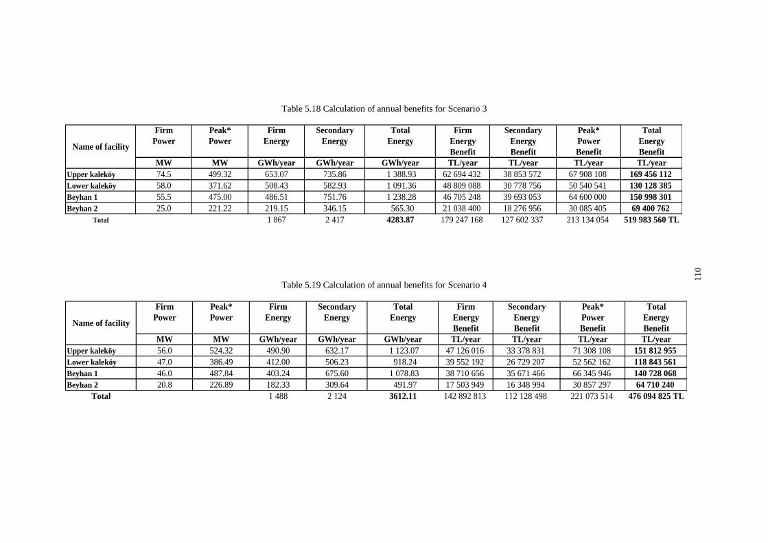
110
Table 5.18 Calculation of annual benefits for Scenario 3
Firm Peak* Firm Secondary Total Firm Secondary Peak* Total
Power Power Energy Energy Energy Energy Energy Power Energy
Benefit Benefit Benefit Benefit
MW MW GWh/year GWh/year GWh/year TL/year TL/year TL/year TL/year
Upper kaleköy 74.5 499.32 653.07 735.86 1 388.93 62 694 432 38 853 572 67 908 108 169 456 112
Lower kaleköy 58.0 371.62 508.43 582.93 1 091.36 48 809 088 30 778 756 50 540 541 130 128 385
Beyhan 1 55.5 475.00 486.51 751.76 1 238.28 46 705 248 39 693 053 64 600 000 150 998 301
Beyhan 2 25.0 221.22 219.15 346.15 565.30 21 038 400 18 276 956 30 085 405 69 400 762
Total 1 867 2 417 4283.87 179 247 168 127 602 337 213 134 054 519 983 560 TL
Name of facility
Table 5.19 Calculation of annual benefits for Scenario 4
Firm Peak* Firm Secondary Total Firm Secondary Peak* Total
Power Power Energy Energy Energy Energy Energy Power Energy
Benefit Benefit Benefit Benefit
MW MW GWh/year GWh/year GWh/year TL/year TL/year TL/year TL/year
Upper kaleköy 56.0 524.32 490.90 632.17 1 123.07 47 126 016 33 378 831 71 308 108 151 812 955
Lower kaleköy 47.0 386.49 412.00 506.23 918.24 39 552 192 26 729 207 52 562 162 118 843 561
Beyhan 1 46.0 487.84 403.24 675.60 1 078.83 38 710 656 35 671 466 66 345 946 140 728 068
Beyhan 2 20.8 226.89 182.33 309.64 491.97 17 503 949 16 348 994 30 857 297 64 710 240
Total 1 488 2 124 3612.11 142 892 813 112 128 498 221 073 514 476 094 825 TL
Name of facility
11
0
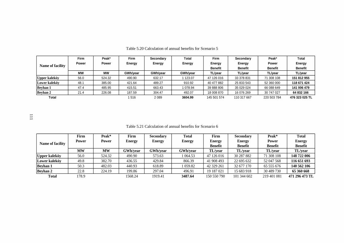
111
Table 5.20 Calculation of annual benefits for Scenario 5
Firm Peak* Firm Secondary Total Firm Secondary Peak* Total
Power Power Energy Energy Energy Energy Energy Power Energy
Benefit Benefit Benefit Benefit
MW MW GWh/year GWh/year GWh/year TL/year TL/year TL/year TL/year
Upper kaleköy 56.0 524.32 490.90 632.17 1 123.07 47 126 016 33 378 831 71 308 108 151 812 955
Lower kaleköy 48.1 385.00 421.64 489.27 910.92 40 477 882 25 833 543 52 360 000 118 671 424
Beyhan 1 47.4 485.95 415.51 663.43 1 078.94 39 888 806 35 029 024 66 088 649 141 006 479
Beyhan 2 21.4 226.08 187.59 304.47 492.07 18 008 870 16 076 269 30 747 027 64 832 166
Total 1 516 2 089 3604.99 145 501 574 110 317 667 220 503 784 476 323 025 TL
Name of facility
Table 5.21 Calculation of annual benefits for Scenario 6
Firm Peak* Firm Secondary Total Firm Secondary Peak* Total
Power Power Energy Energy Energy Energy Energy Power Energy
Benefit Benefit Benefit Benefit
MW MW GWh/year GWh/year GWh/year TL/year TL/year TL/year TL/year
Upper kaleköy 56.0 524.32 490.90 573.63 1 064.53 47 126 016 30 287 882 71 308 108 148 722 006
Lower kaleköy 49.8 382.70 436.55 429.84 866.39 41 908 493 22 695 632 52 047 568 116 651 693
Beyhan 1 50.3 482.03 440.93 618.89 1 059.82 42 329 261 32 677 170 65 555 676 140 562 106
Beyhan 2 22.8 224.19 199.86 297.04 496.91 19 187 021 15 683 918 30 489 730 65 360 668
Total 178.9 1568.24 1919.41 3487.64 150 550 790 101 344 602 219 401 081 471 296 473 TL
Name of facility
11
1

112
Table 5.22 Calculation of annual benefits for Scenario 7
T2 T1 T3 Total T2 T1 T3 Total
18:00 - 24:00 06:00 - 18:00 24:00 - 06:00 Energy 17:00 - 22:00 06:00 - 17:00 22:00 - 06:00 Energy
Benefit Benefit Benefit Benefit
GWh/year GWh/year GWh/year GWh/year TL/year TL/year TL/year TL/year
Upper kalekoy 798.76 379.30 150.95 1329.01 183 411 190 50 561 017 9 638 702 243 610 909
Lower kalekoy 608.25 283.72 118.93 1010.90 139 666 478 37 820 053 7 594 048 185 080 579
Beyhan 1 712.72 355.98 144.10 1212.80 163 653 869 47 452 201 9 201 585 220 307 655
Beyhan 2 323.46 160.82 64.29 548.56 74 272 112 21 437 290 4 104 979 99 814 380
Total 2 443 1 180 478 4101.27 561 003 649 157 270 561 30 539 314 748 813 523 TL
Name of facility
Table 5.23 Calculation of annual benefits for Scenario 8
Pumping T2 T1 T3 Total Pumping T2 T1 T3 Total
24:00 - 06:00 18:00 - 24:00 06:00 - 18:00 24:00 - 06:00 Energy Generated 24:00 - 06:00 17:00 - 22:00 06:00 - 17:00 22:00 - 06:00 Energy
Cost Benefit Benefit Benefit Benefit
GWh/year GWh/year GWh/year GWh/year GWh/year TL/year TL/year TL/year TL/year TL/year
Upper kaleköy -781.02 1 276 531 118 1924.79 - 49 871 794 292 997 132 70 776 146 7 524 078 321 425 562
Lower kaleköy 612 350 96 1058.64 140 604 916 46 671 141 6 141 474 193 417 532
Beyhan 1 681 398 132 1211.02 156 418 893 53 026 993 8 429 756 217 875 642
Beyhan 2 314 180 59 553.60 72 061 098 24 049 384 3 790 195 99 900 677
Total 2 883 1 459 405 4748.05 - 49 871 794 662 082 040 194 523 664 25 885 502 832 619 413 TL
Name of facility
11
2

113
Table 5.24 Calculation of annual benefits for Scenario 9
Pumping T2 T1 T3 Total Pumping T2 T1 T3 Total
24:00 - 06:00 18:00 - 24:00 06:00 - 18:00 24:00 - 06:00 Energy Generated 24:00 - 06:00 17:00 - 22:00 06:00 - 17:00 22:00 - 06:00 Energy
Cost Benefit Benefit Benefit Benefit
GWh/year GWh/year GWh/year GWh/year GWh/year TL/year TL/year TL/year TL/year TL/year
Upper kaleköy 799 379 151 1329.01 183 411 190 50 561 017 9 638 702 243 610 909
Lower kaleköy 608 284 119 1010.90 139 666 478 37 820 053 7 594 048 185 080 579
Beyhan 1 - 581.3 1 159 389 108 1074.93 - 37 118 273 266 172 165 51 844 340 6 903 282 287 801 514
Beyhan 2 336 169 50 554.38 77 156 790 22 497 487 3 166 343 102 820 620
Total 2 902 1 221 428 3969.22 - 37 118 273 666 406 622 162 722 897 27 302 375 819 313 622 TL
Name of facility
Table 5.25 Calculation of annual benefits for Scenario 10
Pumping T2 T1 T3 Total Pumping T2 T1 T3 Total
24:00 - 06:00 18:00 - 24:00 06:00 - 18:00 24:00 - 06:00 Energy Generated 24:00 - 06:00 17:00 - 22:00 06:00 - 17:00 22:00 - 06:00 Energy
Cost Benefit Benefit Benefit Benefit
GWh/year GWh/year GWh/year GWh/year GWh/year TL/year TL/year TL/year TL/year TL/year
Upper kalekoy - 781.0 1 276 531 118 1143.78 - 49 871 794 292 997 132 70 776 146 7 524 078 321 425 562
Lower kalekoy 612 350 96 1058.64 140 604 916 46 671 141 6 141 474 193 417 532
Beyhan 1 - 683.8 1 176 444 110 1047.01 - 43 664 109 270 028 540 59 238 775 7 051 391 292 654 597
Beyhan 2 312 188 51 550.71 71 644 238 25 064 513 3 235 392 99 944 144
Total 3 376 1 514 375 3800.13 - 93 535 903 775 274 826 201 750 576 23 952 335 907 441 834 TL
Name of facility
11
3
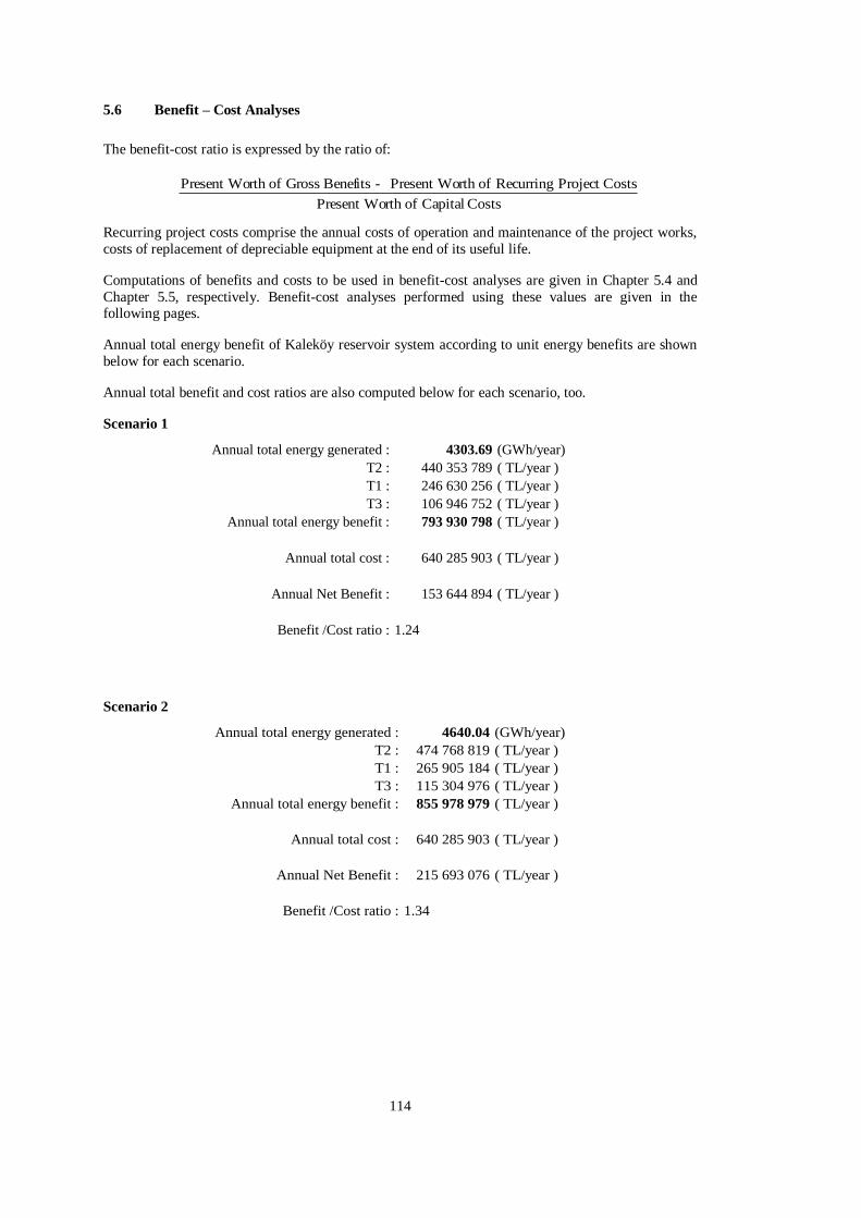
114
5.6 Benefit – Cost Analyses
The benefit-cost ratio is expressed by the ratio of:
Recurring project costs comprise the annual costs of operation and maintenance of the project works,
costs of replacement of depreciable equipment at the end of its useful life.
Computations of benefits and costs to be used in benefit-cost analyses are given in Chapter 5.4 and
Chapter 5.5, respectively. Benefit-cost analyses performed using these values are given in the following pages.
Annual total energy benefit of Kaleköy reservoir system according to unit energy benefits are shown
below for each scenario.
Annual total benefit and cost ratios are also computed below for each scenario, too.
Scenario 1
4303.69 (GWh/year)
T2 : 440 353 789 ( TL/year )
T1 : 246 630 256 ( TL/year )
T3 : 106 946 752 ( TL/year )
793 930 798 ( TL/year )
640 285 903 ( TL/year )
Annual Net Benefit : 153 644 894 ( TL/year )
Benefit /Cost ratio : 1.24
Annual total energy generated :
Annual total energy benefit :
Annual total cost :
Scenario 2
4640.04 (GWh/year)
T2 : 474 768 819 ( TL/year )
T1 : 265 905 184 ( TL/year )
T3 : 115 304 976 ( TL/year )
855 978 979 ( TL/year )
640 285 903 ( TL/year )
Annual Net Benefit : 215 693 076 ( TL/year )
Benefit /Cost ratio : 1.34
Annual total energy generated :
Annual total energy benefit :
Annual total cost :
Costs Capital ofrth Present Wo
CostsProject Recurring ofrth Present Wo - Benefits Gross ofrth Present Wo

115
Scenario 3
4283.87 (GWh/year)
179 247 168 ( TL/year )
127 602 337 ( TL/year )
213 134 054 ( TL/year )
519 983 560 ( TL/year )
640 285 903 ( TL/year )
Annual Net Benefit : -120 302 344 ( TL/year )
Benefit/Cost ratio : 0.81
Annual total cost:
Annual firm energy benefit:
Annual secondary energy benefit:
Annual peak energy benefit:
Annual total energy generated:
Annual total energy benefit:
Scenario 4
3612.11 (GWh/year)
142 892 813 ( TL/year )
112 128 498 ( TL/year )
221 073 514 ( TL/year )
476 094 825 ( TL/year )
640 285 903 ( TL/year )
Annual Net Benefit : -164 191 079 ( TL/year )
Benefit/Cost ratio : 0.74
Annual firm energy benefit:
Annual secondary energy benefit:
Annual peak energy benefit:
Annual total energy generated:
Annual total energy benefit:
Annual total cost:
Scenario 5
3604.99 (GWh/year)
145 501 574 ( TL/year )
110 317 667 ( TL/year )
220 503 784 ( TL/year )
476 323 025 ( TL/year )
640 285 903 ( TL/year )
Annual Net Benefit : -163 962 879 ( TL/year )
Benefit/Cost ratio : 0.74
Annual firm energy benefit:
Annual secondary energy benefit:
Annual peak energy benefit:
Annual total energy generated:
Annual total energy benefit:
Annual total cost:
Scenario 6
3487.64 (GWh/year)
150 550 790 ( TL/year )
101 344 602 ( TL/year )
219 401 081 ( TL/year )
471 296 473 ( TL/year )
640 285 903 ( TL/year )
Annual Net Benefit : -168 989 430 ( TL/year )
Benefit/Cost ratio : 0.74
Annual firm energy benefit:
Annual secondary energy benefit:
Annual peak energy benefit:
Annual total energy generated:
Annual total energy benefit:
Annual total cost:
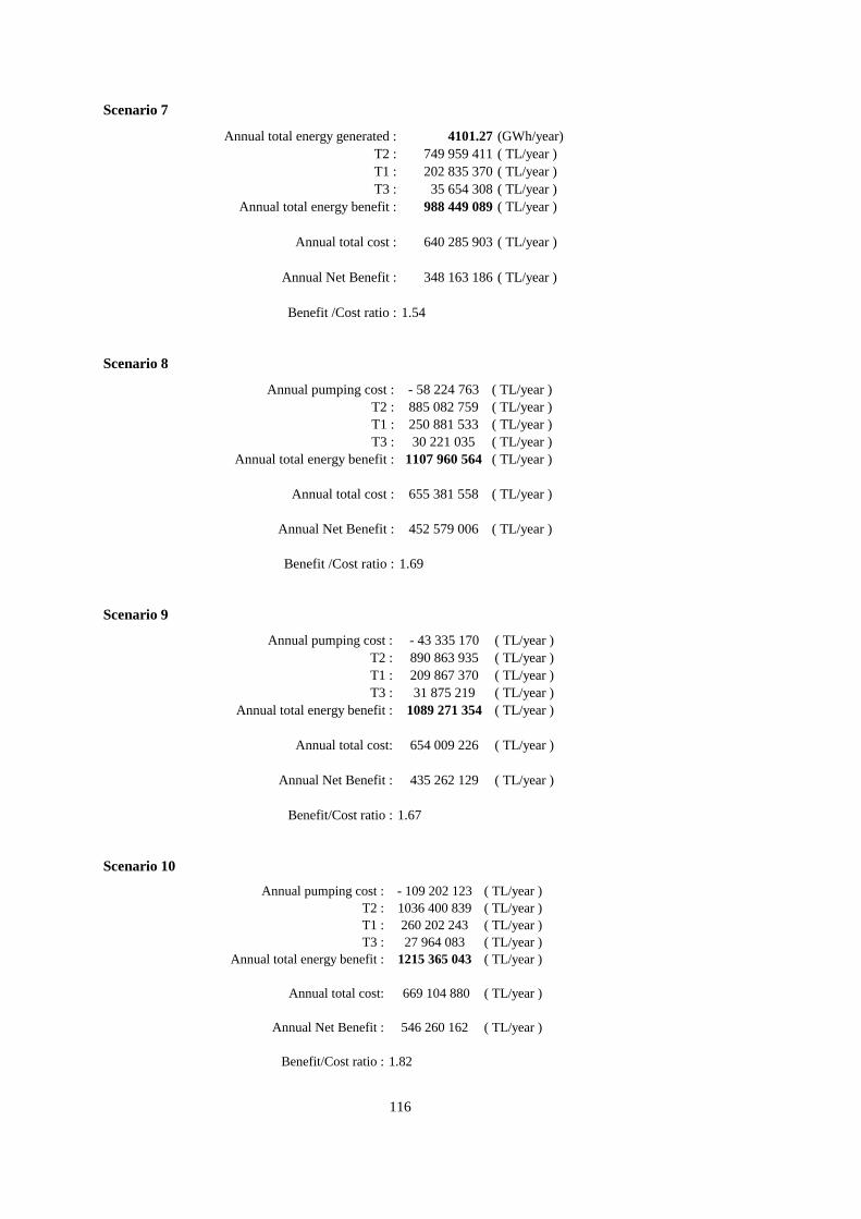
116
Scenario 7
4101.27 (GWh/year)
T2 : 749 959 411 ( TL/year )
T1 : 202 835 370 ( TL/year )
T3 : 35 654 308 ( TL/year )
988 449 089 ( TL/year )
640 285 903 ( TL/year )
Annual Net Benefit : 348 163 186 ( TL/year )
Benefit /Cost ratio : 1.54
Annual total energy generated :
Annual total energy benefit :
Annual total cost :
Scenario 8
- 58 224 763 ( TL/year )
T2 : 885 082 759 ( TL/year )
T1 : 250 881 533 ( TL/year )
T3 : 30 221 035 ( TL/year )
1107 960 564 ( TL/year )
655 381 558 ( TL/year )
Annual Net Benefit : 452 579 006 ( TL/year )
Benefit /Cost ratio : 1.69
Annual pumping cost :
Annual total energy benefit :
Annual total cost :
Scenario 9
- 43 335 170 ( TL/year )
T2 : 890 863 935 ( TL/year )
T1 : 209 867 370 ( TL/year )
T3 : 31 875 219 ( TL/year )
1089 271 354 ( TL/year )
654 009 226 ( TL/year )
Annual Net Benefit : 435 262 129 ( TL/year )
Benefit/Cost ratio : 1.67
Annual pumping cost :
Annual total energy benefit :
Annual total cost:
Scenario 10
- 109 202 123 ( TL/year )
T2 : 1036 400 839 ( TL/year )
T1 : 260 202 243 ( TL/year )
T3 : 27 964 083 ( TL/year )
1215 365 043 ( TL/year )
669 104 880 ( TL/year )
Annual Net Benefit : 546 260 162 ( TL/year )
Benefit/Cost ratio : 1.82
Annual pumping cost :
Annual total energy benefit :
Annual total cost:

117
5.7 Internal Rate of Return
The Internal Rate of Return (IRR) refers to the discount rate, for which, considered the given study
period, the Net Present Value is zero (NPV = 0). In other words, internal rate of return is the interest-discount rate that equates the present worth values of all annual costs and benefits throughout the
economic life of the project. IRR describes to what extent the investment delivers a higher discount
rate than the selected discount rate i representing capital cost. The necessary requirement for the
investment to be accepted is that IRR > i.
where,
Rt = annual revenues resulted from the sale of electricity (TL/year),
It = annual investment (TL/year),
Ct = annual operating related costs (TL/year),
n = 4 years of project development and 50 years of operation.
Graphs of cash flow and the computations of internal rate of return of the scenarios are given in
Appendix A.
In the computations, net income loss due to expropriation has been added to annual costs. This value
has been obtained from Feasibility Report as 4 240 000 TL (Temelsu International Engineering
Services Inc., 2011).
Internal rate of return values for Kaleköy reservoir system are summarized from Tables A1-A10 and
illustrated in Table 5.26.
Table 5.26 Internal rate of return values for Scenarios
Internal rate of return (%)
Scenario 1 12.21
Scenario 2 13.08
Scenario 3 8.05
Scenario 4 7.31
Scenario 5 7.31
Scenario 6 7.23
Scenario 7 14.85
Scenario 8 16.06
Scenario 9 15.85
Scenario 10 17.07
(5.2) 0)1(
)(
1
n
tt
ttt
IRR
CIR

118

119
CHAPTER 6
DISCUSSION OF RESULTS
6.1 Discussion of Results
The economic feasibility of the Kaleköy reservoir system is evaluated on the basis of its internal rate
of return and also, for a selected discount rate, on the basis of the present worth of net benefits and the
benefit-cost ratio.
Various scenarios provide different insight into the economics of the project. The internal rate of
return gives the average annual return on the investment. It is the only parameter which is independent of the selection of a discount rate at which fully accounts for the phasing of costs and benefits. The
internal rate of return is the discount rate at which the project shows a benefit-cost ratio of unity. In
Figure 6.1, internal rate of return values of the scenarios are presented. Scenario 10 with two pumped
power plants has the highest internal rate of return value.
0
1
2
3
4
5
6
7
8
9
10
11
12
13
14
15
16
17
18
1 2 3 4 5 6 7 8 9 10
Rate of Return
Scenario 1 Scenario 2 Scenario 3 Scenario 4 Scenario 5
Scenario 6 Scenario 7 Scenario 8 Scenario 9 Scenario 10
Perc
en
t (%
)
Figure 6.1 Internal rate of return values (%) for Scenarios
The reservoirs are operated at the full operation level (i.e. no usage of operation guide curves) in the
Scenario 1. The results for the energy generation for the Scenario 1 is that mean power generation is
computed to be 490.9 MW, which is equivalent to an annual energy generation of 4303.7 GWh. For

120
the other design scenarios the annual energy generation ranges from 3488 GWh to 4640 GWh as
shown in Figure 6.2.
In Scenario 2, 10% percent increase in the inflows of Kaleköy reservoir system is applied to the simulation model. The results for the energy and revenue generation of the Scenario 2 is less than
10% percent compared to Scenario 1 as shown in Figure 6.1 and 6.2.
Firm energy is the minimum output which can be guaranteed if no worse hydrological conditions
occur than those represented by the flow data of the critical period. The critical period has also been
investigated for the case that "firm" energy is produced according to a given non-uniform pattern, as
was explained in sections 3.4 and 3.5. In Scenario 3 and 4, if we consider firm energy requirement it
results decrease in annual energy generation and benefits since operation head is not usually at
maximum level. However, there is a 22% decrease in inflow in Scenario 4 due to full development case inflows, reduction in energy generation is 16%.
In this thesis, the official unit prices of firm and secondary energies and the discount ratio advocated
by the General Directorate of State Water Works is used as 6 and 3.3 US Cents/kWh, respectively
which are unrealistically too low. In Chapter 5 the present worth of benefits of the Kaleköy reservoir
system is computed using these values. In Scenario 3, the sensitivity of the present worth of benefits
on the unit prices is quantitatively analyzed by making the unit prices 10 and 5 US Cents/kWh than it
is observed that the benefit/cost ratio increases to 1.1.
Besides, for a given discount rate the benefit-costs ratio indicates the profitability of the project and
the present worth of net benefits reflects the size of the profits. In order for these economic parameters
to provide a valid basis for scenario evaluation, the selected discount rate (9.5%) must reflect the true
value of capital in the Turkish economy. Sensitivity analyses may be performed for different discount
rates as well.
The effect of the increase in conservation volume on power generation is investigated in Scenario 5.
The minimum storage level indicated on the designs has been selected in a way that is above dead
storage and vortex limitations. In the case of Lower Kaleköy Reservoir, this design minimum is
lowered in Scenario 5. When we compare Scenario 4 and Scenario 5, results show that there is almost
no difference in energy generation at Upper Kaleköy since no change made on upstream network. In
addition to this, only 2% increase in total firm energy generation, is achieved.
3000310032003300340035003600370038003900400041004200430044004500460047004800
1 2 3 4 5 6 7 8 9 10
Annual Total Energy
Scenario 1 Scenario 2 Scenario 3 Scenario 4 Scenario 5
Scenario 6 Scenario 7 Scenario 8 Scenario 9 Scenario 10
An
nu
al T
ota
l En
erg
y G
en
era
tio
n (G
Wh
/yea
r)
Figure 6.2 Annual Total Energy Generation (GWh/year) for Scenarios
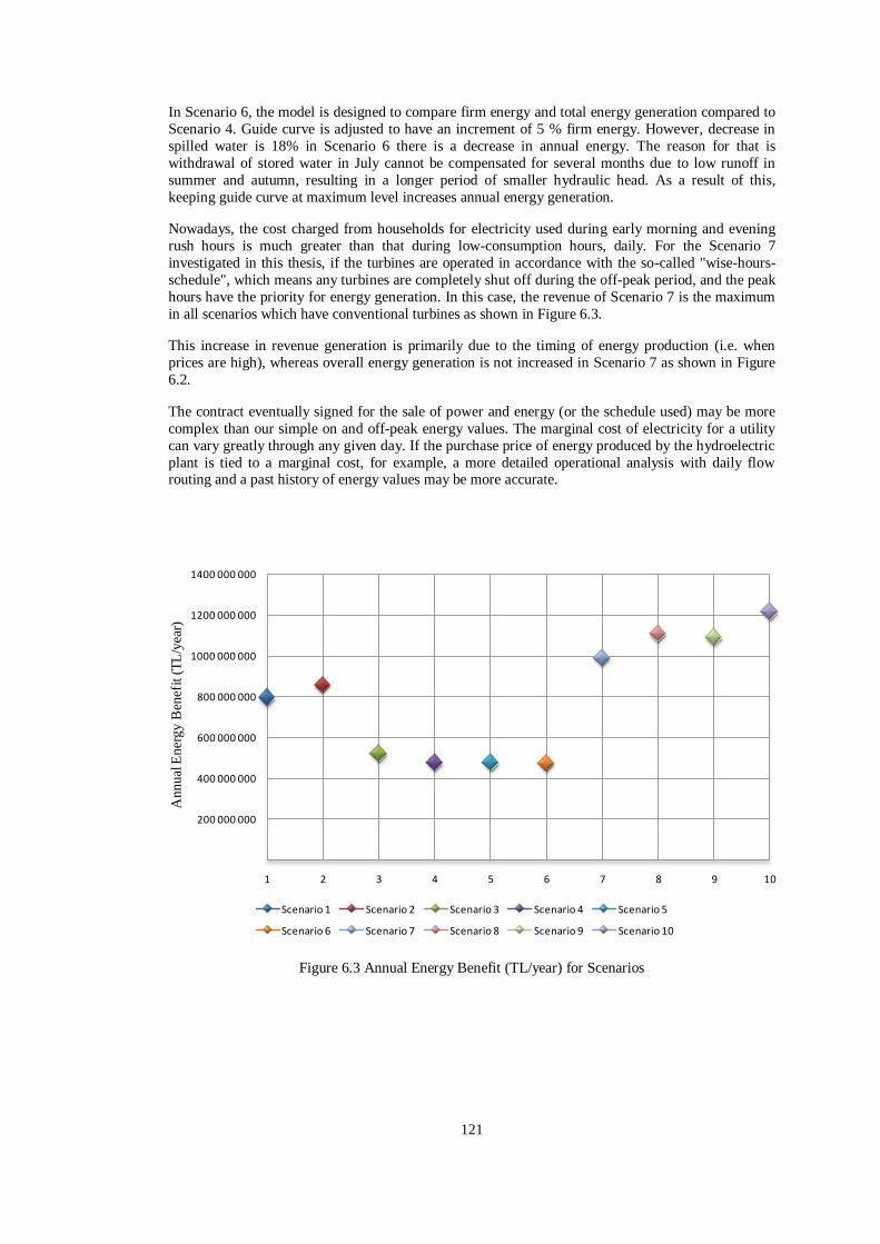
121
In Scenario 6, the model is designed to compare firm energy and total energy generation compared to
Scenario 4. Guide curve is adjusted to have an increment of 5 % firm energy. However, decrease in
spilled water is 18% in Scenario 6 there is a decrease in annual energy. The reason for that is
withdrawal of stored water in July cannot be compensated for several months due to low runoff in
summer and autumn, resulting in a longer period of smaller hydraulic head. As a result of this,
keeping guide curve at maximum level increases annual energy generation.
Nowadays, the cost charged from households for electricity used during early morning and evening
rush hours is much greater than that during low-consumption hours, daily. For the Scenario 7
investigated in this thesis, if the turbines are operated in accordance with the so-called "wise-hours-
schedule", which means any turbines are completely shut off during the off-peak period, and the peak
hours have the priority for energy generation. In this case, the revenue of Scenario 7 is the maximum
in all scenarios which have conventional turbines as shown in Figure 6.3.
This increase in revenue generation is primarily due to the timing of energy production (i.e. when
prices are high), whereas overall energy generation is not increased in Scenario 7 as shown in Figure
6.2.
The contract eventually signed for the sale of power and energy (or the schedule used) may be more
complex than our simple on and off-peak energy values. The marginal cost of electricity for a utility
can vary greatly through any given day. If the purchase price of energy produced by the hydroelectric
plant is tied to a marginal cost, for example, a more detailed operational analysis with daily flow routing and a past history of energy values may be more accurate.
200 000 000
400 000 000
600 000 000
800 000 000
1000 000 000
1200 000 000
1400 000 000
1 2 3 4 5 6 7 8 9 10
Annual Energy Benefit (TL)
Scenario 1 Scenario 2 Scenario 3 Scenario 4 Scenario 5
Scenario 6 Scenario 7 Scenario 8 Scenario 9 Scenario 10
An
nual
En
erg
y B
enef
it (T
L/y
ear)
Figure 6.3 Annual Energy Benefit (TL/year) for Scenarios

122
00.10.20.30.40.50.60.70.80.9
11.11.21.31.41.51.61.71.81.9
2
1 2 3 4 5 6 7 8 9 10
Benefit/Cost Ratio
Scenario 1 Scenario 2 Scenario 3 Scenario 4 Scenario 5
Scenario 6 Scenario 7 Scenario 8 Scenario 9 Scenario 10
Ben
efit
/Cost
Rat
ios
Figure 6.4 Benefit/Cost Ratios for Scenarios
The rising demand for peaking power is creating a completely new market value, which is also
increasing the attractiveness of pumped storage power stations. In Scenario 8, 9 and 10 pumped
storage scenarios have been analyzed.
The costs and benefits of power and energy production have been evaluated over a period of fifty years and the benefit/cost ratios are determined in Chapter 5. In Figure 6.4, pumped storage scenarios
have the maximum benefit/cost ratio over all scenarios.
According to the above given benefit/cost ratios in Figure 6.4 and unit energy prices, pump storage
alternative seems feasible. Scenario 10 has the maximum benefit/cost ratio over all scenarios with two
reversible turbines. These results demonstrate the increasing attractiveness of the Kaleköy reservoir
system with pump turbines. In addition to this, it is quite sensitive to the energy unit prices and
working hours in pump and turbine modes. The analyses have been performed according to the accepted current unit prices which are subject to change either in short term or long term. Therefore it
will be beneficial to re-evaluate pump storage alternative after carrying out a projection study in
energy prices to decide if it is feasible or not.
Annual total energy generation in pumped storage scenarios is below the average values respect to
Scenario 1, 3 and 7 in existing case inflows. Therefore, it is plausible that such an operation of the
reservoirs increases revenue generation, but not energy generation.

123
CHAPTER 7
CONCLUSION AND RECOMMENDATIONS
7.1 Conclusion
In production of electrical energy, compared to fossil and nuclear thermal plants, natural gas-fired
power plants; hydroelectric power plants have two important properties such as renewable source and
peak operation. Consumption of electrical energy is one of the most important indicators of economic
development and social well-being. Electricity production or consumption per capita of any country is
one of the indicators of the living standart.
The growing demand for electricity in Turkey will require the addition of large increments of
generating capacity to supply the interconnected system. Hydro-electric power plants on the Murat
River are logical and economical sources of power and their development through the construction of
dams on the Murat forms an integral part of the national long range power development plan.
Hydropower can be used in a power system in several ways: for peaking, for meeting intermediate
loads, for base load operation, or for meeting a combination of these loads. These alternative
operations is illustrated in the previous chapters.
Instead of energy production using foreign dependent fuel as natural gas and imported coal, Turkey
has to give priority to and realize energy production using local resources as hydropower in order to
lessen the foreign dependency.
Feasibility report for Lower Fırat basin was carried out in 2011 by Pöyry and Temelsu International
Engineering Services Inc. in order to investigate the potential for exploiting the hydro-electric
potential of the river system. Maximization of firm energy and operation of reservoirs in peak mode
were studied in the feasibility study.
In this thesis the feasibility report is improved by considering different operation scenarios and
pumped storage alternatives. Scenarios and the financial analysis are described regarding the
hydropower potential in the previous chapters.
Kaleköy reservoir system, located upstream of the Keban Dam, will utilise the hydro potential of the Murat river between the elevations of 870 m and 1225 m in four powerplants totalling 1705 MW of
installed capacity.
HEC-ResSim simulation program is used to model the cascade reservoir system. Analysis of the
complex system is easy to model by using the HEC-ResSim. In order to minimize spillage during high
flow season and to benefit from a higher head various operation rules have been defined.
Pumped storage applications are investigated as well. Pumped storage hydroelectricity is the only
economic and flexible means of storing grid scale amounts of excess energy, allowing power plants
dispatchers to successfully manage that balancing act. This is becoming even more important as more
and more countries are building up their power generation from intermittent renewables such as wind
and solar.
The advantage of this technology is that it can come online very quickly, making it a useful tool to
balance the varying electricity demand from consumers or unplanned outages of other power plants.

124
In recent years, the profitability of pumped storage plants has increased as a consequence of increased
price volatility on electricity spot markets.
A financial assessment was carried out for the full range of ten scenarios, in order to assess the cost effective operation regime and the economic feasibility of the scenarios. Ten scenarios are made of
the type of operation required in order to reduce spillage and maintain high water levels in the
reservoir. The results of the scenarios show that the Kaleköy Reservoir System is profitable. However,
choosing an appropriate operation is more delicate, particularly as measuring future demand for peak
energy or fluctuations in the electricity price is uncertain.
The scenarios related to evaluation indicators are the internal rate of return and the benefit-cost ratio,
which provide information on the degree of profitability of the scenarios. From the current analysis,
Scenario 7 and scenarios with reversible pump turbines seem to give the best internal rate of return and benefit-cost ratios.
7.2 Recommendations
In developing an operational procedure, one may also want to consider the stochastic nature of the
flow; i.e., it is useful to remember that the future is not an exact replica of the past. Uncertainty must be taken into account in the forecasts. Once means of achieving this would be to generate a number of
flow forecasts, each with a given probability of occurrence, and in an operation routine one should
consider all the forecasts and their probabilities. For this reason the rules for the operation of the
reservoirs derived from present conditions must be considered flexible and subject to minor changes
as future events and operating experience may dictate.
Sensitivity scenarios should be considered for capital cost over runs and increased operation costs,
and a reduction on generation over the life of the plant. The necessity for sensitivity scenarios for electricity prices should be simulated.
During the winter season, the watershed is covered by snow. Snowmelt is significant part of the river
flow in the spring season. A snow hydrology model of the basin using available ground and remotely
sensed data should be developed to better understand the water resources in the Upper Fırat Basin.
The snow model may accurately model snow accumulation and melt and can provide useful
information about the snow hydrology of the region. Reservoir managers can use this information in
operating decisions, to maximize water supply.
The revenues are all related to the sales of electricity only. The sales price rates are expected to be the
prices at the moment of the commissioning of the power plant. Projections in energy prices and peak
hours should be considered in other scenarios. An increase of the energy price may be expected to
occur during the lifetime of the Kaleköy Reservoir System. The financial viability of the project
should be assessed more precisely in a specific economic model. An economic model for future unit
energy prices will be essential for more accurate results.
It is essential to formulate the operation rules with information that will be available at the time when
operation decisions are made. If forecasts are used in operation, the degree of reliability must be taken
into account in deriving operating rules. In assessing the benefits that would be associated with a
particular set of operating rules, forecast errors must be simulated in such a manner as to represent
average anticipated accomplishment under those rules.
Watershed development plans prepared at different times may become inconsistent because of the
economic point of view at later dates. However, some preliminary studies have been abandoned,
within the time according to the changes occurring in the energy benefits and economic costs of
facilities of the same projects may be feasible. For this reason, at certain intervals watershed
development plans should be revised.

125
BIBLIOGRAPHY
Alantor, D.D., Malkoç, F., Bektaşoğlu, B. and Eminoğlu, E., Efficiency in Reservoir Operation,
With International Participation Third National Symposium on Dam Safety, Eskişehir, 2012, pp 359-366 (in Turkish).
ASCE, Guidelines for Design of Intakes for Hydroelectric Plants, New York, 1995.
Bakır, N., http://www.ere.com.tr/EMO_21Aralik2005.pdf, last visited on January 2013.
Deloitte Financial Advisory Services LLP, Turkish Electricity Market: Developments and
Expectations 2010-2011, 2010.
Doland, J.J., Hydro Power Engineering, The Roland Press Company, New York, 1954.
Dyson, M., Bergkamp, G. and Scanlon, J., The essentials of environmental flows, The World
Conversation Union, UK, 2003.
EM 1110-2-1701, Engineering and Design Hydropower, Engineering Manual, Washington, 1985.
Energy Market Regulatory Authority, Electricity Market Report 2010, Ankara, 2011.
Energy Market Regulatory Authority, Electricity Market Report 2011, Ankara, 2012.
General Directorate of Renewable Energy, http://www.eie.gov.tr/yenilenebilir/
h_turkiye_potansiyel.aspx, last visited on December 2012.
Gulliver, J.S. and Arndt, R.E.A., Hydropower Engineering Handbook, McGraw-Hill Inc., 1991.
International Energy Agency, World Energy Outlook 2012, 2012.
Investment Support and Promotion Agency, Turkey’s Energy Sector Report, Deloitte, 2010.
İnci, K.O., Hydroelectric Power Plant Investments and Technologies, International Energy
Congress and Fair, Ankara, 2012.
Jefferies, D.G., Institution of Civil Engineers, Pumped Storage, Thomas Telford, London, 1990.
Kansal, M.L., System Analysis Techniques in Water Resources Management, Turkish Water
Foundation, Istanbul, 2005.
Klipsch, J.D., HEC-ResSim Reservoir System Simulation – User’s Manual Version 3.0, U.S.
Army Corps of Engineers Hydrologic Engineering Center, Davis, 2007.
Lempérière, F., Global overview of pumped storage potential and cost, Hydro Conference Papers,
2011, pp 18.01.
Miller, R., Opportunities in Pumped Storage Hydropower, Power Engineering Magazine, 2010,
pp 50-52.
Mitteregger, A., Austrian pumped storage power stations supply peak demands, World Pump
Magazine, 2008.
Nandalal, K.D.W. and Bogardi, J.J., Dynamic Programming Based Operation of Reservoirs:
Applicability and Limits, Cambridge University Press, 2007.

126
Oliveira, M.A., Venda Nova III repowering project, Hydro Conference Papers, 2011, pp 15.03.
Özbakır, B., Modelling of Seyhan and Ceyhan River Basin with Using HEC-ResSim Program,
M.Sc.Thesis, Department of Civil Engineering, Gazi University, 2009.
Rukuni, S., Modeling the response of small multi-purpose reservoirs to hydrology for improved
rural livelihoods in the Mzingwane catchment: Limpopo Basin, M.Sc.Thesis, Department of Civil
Engineering, Zimbabwe University, 2006.
Saraç, M., The First Hydroelectric Power Plant Projects in Turkey, With International Participation Third National Symposium on Dam Safety, Eskişehir, 2012, pp 161-168 (in
Turkish).
Saraç, M., Pumped Storage Hydroelectric Power Plants, With International Participation Third
National Symposium on Dam Safety, Eskişehir, 2012, pp 459-470.
Temelsu International Engineering Services Inc., Lower Murat Basin Final Feasibility Report,
2011.
Turkish Electricity Distribution Company, http://www.tedas.gov.tr/274,2012_ Tarifeler.html, last
visited on December 2012.
Turkish Electricity Transmission Company, Turkish Electrical Energy 10-Year Generation
Capacity Projection (2011-2020), Ankara, 2011.
University of Texas, http://www.crwr.utexas.edu/gis/gishyd98/dhi/mikebas/ Mbasmain.htm, last
visited on December 2012.
Voith, Pumped Storage Machines, Turbine Catalogs and Manuals, Germany, 2009.
Yanmaz, A.M., Applied Water Resources Engineering, METU Press Publishing Co., Ankara,
2006.
Zhang, H., Xia, Xiaohua., Zhang, Jiangfeng., Optimal sizing and operation of pumping systems to
achieve energy efficiency and load shifting, Electric Power Systems Research 86, Elsevier, 2012,
pp 41-50.
World Map, http://mapas.owje.com/maps/8725_eastern-turkey-and-vicinity-shaded-relief-
map.htm, last visited on December 2012.

127
APPENDIX A
INTERNAL RATE OF RETURN CALCULATIONS
Table A.1 Internal rate of return for Scenario 1
Year Costs Benefits Net Benefit Net Present Value
1 1 116 861 429 -1 116 861 429 -1054 325 472
2 1 836 796 576 -1 836 796 576 -1545 209 181
3 1 209 117 607 -1 209 117 607 -906 453 597
4 758 246 723 - 758 246 723 -506 568 740
5 57 997 019 793 930 798 735 933 779 438 144 530
6 57 997 019 793 930 798 735 933 779 390 452 499
7 57 997 019 793 930 798 735 933 779 347 951 745
8 57 997 019 793 930 798 735 933 779 310 077 198
9 57 997 019 793 930 798 735 933 779 276 325 296
10 57 997 019 793 930 798 735 933 779 246 247 288
11 57 997 019 793 930 798 735 933 779 219 443 272
12 57 997 019 793 930 798 735 933 779 195 556 872
13 57 997 019 793 930 798 735 933 779 174 270 507
14 57 997 019 793 930 798 735 933 779 155 301 163
15 57 997 019 793 930 798 735 933 779 138 396 631
16 57 997 019 793 930 798 735 933 779 123 332 158
17 57 997 019 793 930 798 735 933 779 109 907 453
18 57 997 019 793 930 798 735 933 779 97 944 027
19 57 997 019 793 930 798 735 933 779 87 282 820
20 57 997 019 793 930 798 735 933 779 77 782 085
21 57 997 019 793 930 798 735 933 779 69 315 506
22 57 997 019 793 930 798 735 933 779 61 770 513
23 57 997 019 793 930 798 735 933 779 55 046 793
24 57 997 019 793 930 798 735 933 779 49 054 949
25 57 997 019 793 930 798 735 933 779 43 715 318
26 57 997 019 793 930 798 735 933 779 38 956 906
27 57 997 019 793 930 798 735 933 779 34 716 447
28 57 997 019 793 930 798 735 933 779 30 937 562
29 57 997 019 793 930 798 735 933 779 27 570 008
30 57 997 019 793 930 798 735 933 779 24 569 013
31 57 997 019 793 930 798 735 933 779 21 894 676
32 57 997 019 793 930 798 735 933 779 19 511 440
33 57 997 019 793 930 798 735 933 779 17 387 620
34 57 997 019 793 930 798 735 933 779 15 494 978
35 57 997 019 793 930 798 735 933 779 13 808 350
36 57 997 019 793 930 798 735 933 779 12 305 311
37 57 997 019 793 930 798 735 933 779 10 965 878
38 57 997 019 793 930 798 735 933 779 9 772 242
39 57 997 019 793 930 798 735 933 779 8 708 533
40 57 997 019 793 930 798 735 933 779 7 760 610
41 57 997 019 793 930 798 735 933 779 6 915 867
42 57 997 019 793 930 798 735 933 779 6 163 075
43 57 997 019 793 930 798 735 933 779 5 492 224
44 57 997 019 793 930 798 735 933 779 4 894 396
45 57 997 019 793 930 798 735 933 779 4 361 641
46 57 997 019 793 930 798 735 933 779 3 886 876
47 57 997 019 793 930 798 735 933 779 3 463 790
48 57 997 019 793 930 798 735 933 779 3 086 756
49 57 997 019 793 930 798 735 933 779 2 750 763
50 57 997 019 793 930 798 735 933 779 2 451 342
51 57 997 019 793 930 798 735 933 779 2 184 514
52 57 997 019 793 930 798 735 933 779 1 946 729
53 57 997 019 793 930 798 735 933 779 1 734 828
54 57 997 019 793 930 798 735 933 779 1 545 992
7 820 873 279 39 696 539 887 31 875 666 608 0
Internal Rate of Return : 12.21%
Internal Rate of Return

128
Figure A.1 Cash flow graph for Scenario 1
-2 000 000 000
-1 500 000 000
-1 000 000 000
- 500 000 000
500 000 000
1 000 000 000
1 2 3 4 5 6 7 8 9 10 11 12 13 14 15 16 17 18 19 20 21 22 23 24 25 26 27 28 29 30 31 32 33 34 35 36 37 38 39 40 41 42 43 44 45 46 47 48 49 50 51 52 53 54
Tu
rk
ish
Lir
a (
TL
)
Year
Annual benefit
Annual cost
128
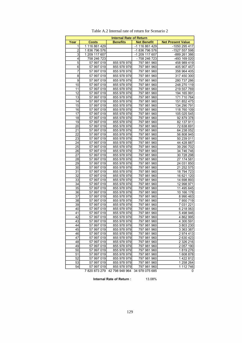
129
Table A.2 Internal rate of return for Scenario 2
Year Costs Benefits Net Benefit Net Present Value
1 1 116 861 429 -1 116 861 429 -1050 295 417
2 1 836 796 576 -1 836 796 576 -1527 557 598
3 1 209 117 607 -1 209 117 607 -889 261 386
4 758 246 723 - 758 246 723 -493 169 020
5 57 997 019 855 978 979 797 981 960 458 989 419
6 57 997 019 855 978 979 797 981 960 405 907 457
7 57 997 019 855 978 979 797 981 960 358 964 405
8 57 997 019 855 978 979 797 981 960 317 450 300
9 57 997 019 855 978 979 797 981 960 280 737 286
10 57 997 019 855 978 979 797 981 960 248 270 119
11 57 997 019 855 978 979 797 981 960 219 557 769
12 57 997 019 855 978 979 797 981 960 194 165 991
13 57 997 019 855 978 979 797 981 960 171 710 764
14 57 997 019 855 978 979 797 981 960 151 852 475
15 57 997 019 855 978 979 797 981 960 134 290 791
16 57 997 019 855 978 979 797 981 960 118 760 109
17 57 997 019 855 978 979 797 981 960 105 025 545
18 57 997 019 855 978 979 797 981 960 92 879 378
19 57 997 019 855 978 979 797 981 960 82 137 911
20 57 997 019 855 978 979 797 981 960 72 638 691
21 57 997 019 855 978 979 797 981 960 64 238 052
22 57 997 019 855 978 979 797 981 960 56 808 945
23 57 997 019 855 978 979 797 981 960 50 239 011
24 57 997 019 855 978 979 797 981 960 44 428 887
25 57 997 019 855 978 979 797 981 960 39 290 702
26 57 997 019 855 978 979 797 981 960 34 746 746
27 57 997 019 855 978 979 797 981 960 30 728 298
28 57 997 019 855 978 979 797 981 960 27 174 581
29 57 997 019 855 978 979 797 981 960 24 031 850
30 57 997 019 855 978 979 797 981 960 21 252 575
31 57 997 019 855 978 979 797 981 960 18 794 723
32 57 997 019 855 978 979 797 981 960 16 621 120
33 57 997 019 855 978 979 797 981 960 14 698 893
34 57 997 019 855 978 979 797 981 960 12 998 971
35 57 997 019 855 978 979 797 981 960 11 495 645
36 57 997 019 855 978 979 797 981 960 10 166 178
37 57 997 019 855 978 979 797 981 960 8 990 463
38 57 997 019 855 978 979 797 981 960 7 950 719
39 57 997 019 855 978 979 797 981 960 7 031 221
40 57 997 019 855 978 979 797 981 960 6 218 063
41 57 997 019 855 978 979 797 981 960 5 498 946
42 57 997 019 855 978 979 797 981 960 4 862 995
43 57 997 019 855 978 979 797 981 960 4 300 591
44 57 997 019 855 978 979 797 981 960 3 803 230
45 57 997 019 855 978 979 797 981 960 3 363 387
46 57 997 019 855 978 979 797 981 960 2 974 413
47 57 997 019 855 978 979 797 981 960 2 630 423
48 57 997 019 855 978 979 797 981 960 2 326 216
49 57 997 019 855 978 979 797 981 960 2 057 190
50 57 997 019 855 978 979 797 981 960 1 819 276
51 57 997 019 855 978 979 797 981 960 1 608 878
52 57 997 019 855 978 979 797 981 960 1 422 812
53 57 997 019 855 978 979 797 981 960 1 258 264
54 57 997 019 855 978 979 797 981 960 1 112 746
7 820 873 279 42 798 948 964 34 978 075 685 0
13.08%
Internal Rate of Return
Internal Rate of Return :

130
Figure A.2 Cash flow graph for Scenario 2
-2 000 000 000
-1 500 000 000
-1 000 000 000
- 500 000 000
500 000 000
1 000 000 000
1 2 3 4 5 6 7 8 9 10 11 12 13 14 15 16 17 18 19 20 21 22 23 24 25 26 27 28 29 30 31 32 33 34 35 36 37 38 39 40 41 42 43 44 45 46 47 48 49 50 51 52 53 54
Tu
rk
ish
Lir
a (
TL
)
Year
Annual benefit
Annual cost
13
0

131
Table A.3 Internal rate of return for Scenario 3
Year Costs Benefits Net Benefit Net Present Value
1 1 116 861 429 -1 116 861 429 -1 074 442 234
2 1 836 796 576 -1 836 796 576 -1 635 356 332
3 1 209 117 607 -1 209 117 607 - 996 293 824
4 758 246 723 - 758 246 723 - 578 225 170
5 57 997 019 519 983 560 461 986 541 326 049 344
6 57 997 019 519 983 560 461 986 541 301 752 507
7 57 997 019 519 983 560 461 986 541 279 266 244
8 57 997 019 519 983 560 461 986 541 258 455 633
9 57 997 019 519 983 560 461 986 541 239 195 805
10 57 997 019 519 983 560 461 986 541 221 371 198
11 57 997 019 519 983 560 461 986 541 204 874 862
12 57 997 019 519 983 560 461 986 541 189 607 814
13 57 997 019 519 983 560 461 986 541 175 478 449
14 57 997 019 519 983 560 461 986 541 162 401 989
15 57 997 019 519 983 560 461 986 541 150 299 973
16 57 997 019 519 983 560 461 986 541 139 099 785
17 57 997 019 519 983 560 461 986 541 128 734 223
18 57 997 019 519 983 560 461 986 541 119 141 091
19 57 997 019 519 983 560 461 986 541 110 262 829
20 57 997 019 519 983 560 461 986 541 102 046 165
21 57 997 019 519 983 560 461 986 541 94 441 798
22 57 997 019 519 983 560 461 986 541 87 404 099
23 57 997 019 519 983 560 461 986 541 80 890 843
24 57 997 019 519 983 560 461 986 541 74 862 946
25 57 997 019 519 983 560 461 986 541 69 284 243
26 57 997 019 519 983 560 461 986 541 64 121 257
27 57 997 019 519 983 560 461 986 541 59 343 012
28 57 997 019 519 983 560 461 986 541 54 920 837
29 57 997 019 519 983 560 461 986 541 50 828 197
30 57 997 019 519 983 560 461 986 541 47 040 536
31 57 997 019 519 983 560 461 986 541 43 535 127
32 57 997 019 519 983 560 461 986 541 40 290 938
33 57 997 019 519 983 560 461 986 541 37 288 501
34 57 997 019 519 983 560 461 986 541 34 509 804
35 57 997 019 519 983 560 461 986 541 31 938 171
36 57 997 019 519 983 560 461 986 541 29 558 174
37 57 997 019 519 983 560 461 986 541 27 355 532
38 57 997 019 519 983 560 461 986 541 25 317 028
39 57 997 019 519 983 560 461 986 541 23 430 431
40 57 997 019 519 983 560 461 986 541 21 684 421
41 57 997 019 519 983 560 461 986 541 20 068 522
42 57 997 019 519 983 560 461 986 541 18 573 038
43 57 997 019 519 983 560 461 986 541 17 188 996
44 57 997 019 519 983 560 461 986 541 15 908 091
45 57 997 019 519 983 560 461 986 541 14 722 637
46 57 997 019 519 983 560 461 986 541 13 625 523
47 57 997 019 519 983 560 461 986 541 12 610 164
48 57 997 019 519 983 560 461 986 541 11 670 468
49 57 997 019 519 983 560 461 986 541 10 800 798
50 57 997 019 519 983 560 461 986 541 9 995 934
51 57 997 019 519 983 560 461 986 541 9 251 049
52 57 997 019 519 983 560 461 986 541 8 561 671
53 57 997 019 519 983 560 461 986 541 7 923 664
54 57 997 019 519 983 560 461 986 541 7 333 202
7 820 873 279 25 999 177 977 18 178 304 699 0
Internal Rate of Return : 8.05%
Internal Rate of Return

132
Figure A.3 Cash flow graph for Scenario 3
-2 000 000 000
-1 500 000 000
-1 000 000 000
- 500 000 000
500 000 000
1 000 000 000
1 2 3 4 5 6 7 8 9 10 11 12 13 14 15 16 17 18 19 20 21 22 23 24 25 26 27 28 29 30 31 32 33 34 35 36 37 38 39 40 41 42 43 44 45 46 47 48 49 50 51 52 53 54
Tu
rk
ish
Lir
a (
TL
)
Year
Annual benefit
Annual cost
13
2

133
Table A.4 Internal rate of return for Scenario 4
Year Costs Benefits Net Benefit Net Present Value
1 1 116 861 429 -1 116 861 429 -1 078 146 865
2 1 836 796 576 -1 836 796 576 -1 652 330 639
3 1 209 117 607 -1 209 117 607 -1 013 588 568
4 758 246 723 - 758 246 723 - 592 326 228
5 57 997 019 476 094 825 418 097 806 304 358 597
6 57 997 019 476 094 825 418 097 806 283 623 908
7 57 997 019 476 094 825 418 097 806 264 301 787
8 57 997 019 476 094 825 418 097 806 246 296 002
9 57 997 019 476 094 825 418 097 806 229 516 877
10 57 997 019 476 094 825 418 097 806 213 880 844
11 57 997 019 476 094 825 418 097 806 199 310 029
12 57 997 019 476 094 825 418 097 806 185 731 863
13 57 997 019 476 094 825 418 097 806 173 078 722
14 57 997 019 476 094 825 418 097 806 161 287 586
15 57 997 019 476 094 825 418 097 806 150 299 732
16 57 997 019 476 094 825 418 097 806 140 060 434
17 57 997 019 476 094 825 418 097 806 130 518 698
18 57 997 019 476 094 825 418 097 806 121 627 000
19 57 997 019 476 094 825 418 097 806 113 341 057
20 57 997 019 476 094 825 418 097 806 105 619 601
21 57 997 019 476 094 825 418 097 806 98 424 176
22 57 997 019 476 094 825 418 097 806 91 718 945
23 57 997 019 476 094 825 418 097 806 85 470 513
24 57 997 019 476 094 825 418 097 806 79 647 762
25 57 997 019 476 094 825 418 097 806 74 221 690
26 57 997 019 476 094 825 418 097 806 69 165 274
27 57 997 019 476 094 825 418 097 806 64 453 331
28 57 997 019 476 094 825 418 097 806 60 062 393
29 57 997 019 476 094 825 418 097 806 55 970 591
30 57 997 019 476 094 825 418 097 806 52 157 547
31 57 997 019 476 094 825 418 097 806 48 604 269
32 57 997 019 476 094 825 418 097 806 45 293 062
33 57 997 019 476 094 825 418 097 806 42 207 434
34 57 997 019 476 094 825 418 097 806 39 332 016
35 57 997 019 476 094 825 418 097 806 36 652 489
36 57 997 019 476 094 825 418 097 806 34 155 507
37 57 997 019 476 094 825 418 097 806 31 828 634
38 57 997 019 476 094 825 418 097 806 29 660 281
39 57 997 019 476 094 825 418 097 806 27 639 649
40 57 997 019 476 094 825 418 097 806 25 756 674
41 57 997 019 476 094 825 418 097 806 24 001 979
42 57 997 019 476 094 825 418 097 806 22 366 824
43 57 997 019 476 094 825 418 097 806 20 843 065
44 57 997 019 476 094 825 418 097 806 19 423 113
45 57 997 019 476 094 825 418 097 806 18 099 897
46 57 997 019 476 094 825 418 097 806 16 866 826
47 57 997 019 476 094 825 418 097 806 15 717 759
48 57 997 019 476 094 825 418 097 806 14 646 973
49 57 997 019 476 094 825 418 097 806 13 649 136
50 57 997 019 476 094 825 418 097 806 12 719 277
51 57 997 019 476 094 825 418 097 806 11 852 765
52 57 997 019 476 094 825 418 097 806 11 045 286
53 57 997 019 476 094 825 418 097 806 10 292 816
54 57 997 019 476 094 825 418 097 806 9 591 609
7 820 873 279 23 804 741 237 15 983 867 958 0
7.31%
Internal Rate of Return
Internal Rate of Return :

134
Figure A.4 Cash flow graph for Scenario 4
-2 000 000 000
-1 500 000 000
-1 000 000 000
- 500 000 000
500 000 000
1 000 000 000
1 2 3 4 5 6 7 8 9 10 11 12 13 14 15 16 17 18 19 20 21 22 23 24 25 26 27 28 29 30 31 32 33 34 35 36 37 38 39 40 41 42 43 44 45 46 47 48 49 50 51 52 53 54
Tu
rk
ish
Lir
a (
TL
)
Year
Annual benefit
Annual cost
13
4
2

135
Table A.5 Internal rate of return for Scenario 5
Year Costs Benefits Net Benefit Net Present Value
1 1 116 861 429 -1 116 861 429 -1 078 127 131
2 1 836 796 576 -1 836 796 576 -1 652 239 909
3 1 209 117 607 -1 209 117 607 -1 013 495 808
4 758 246 723 - 758 246 723 - 592 250 340
5 57 997 019 476 323 025 418 326 006 304 474 555
6 57 997 019 476 323 025 418 326 006 283 721 580
7 57 997 019 476 323 025 418 326 006 264 383 127
8 57 997 019 476 323 025 418 326 006 246 362 782
9 57 997 019 476 323 025 418 326 006 229 570 703
10 57 997 019 476 323 025 418 326 006 213 923 171
11 57 997 019 476 323 025 418 326 006 199 342 175
12 57 997 019 476 323 025 418 326 006 185 755 019
13 57 997 019 476 323 025 418 326 006 173 093 963
14 57 997 019 476 323 025 418 326 006 161 295 885
15 57 997 019 476 323 025 418 326 006 150 301 962
16 57 997 019 476 323 025 418 326 006 140 057 386
17 57 997 019 476 323 025 418 326 006 130 511 079
18 57 997 019 476 323 025 418 326 006 121 615 448
19 57 997 019 476 323 025 418 326 006 113 326 143
20 57 997 019 476 323 025 418 326 006 105 601 837
21 57 997 019 476 323 025 418 326 006 98 404 020
22 57 997 019 476 323 025 418 326 006 91 696 805
23 57 997 019 476 323 025 418 326 006 85 446 754
24 57 997 019 476 323 025 418 326 006 79 622 706
25 57 997 019 476 323 025 418 326 006 74 195 625
26 57 997 019 476 323 025 418 326 006 69 138 454
27 57 997 019 476 323 025 418 326 006 64 425 979
28 57 997 019 476 323 025 418 326 006 60 034 706
29 57 997 019 476 323 025 418 326 006 55 942 743
30 57 997 019 476 323 025 418 326 006 52 129 687
31 57 997 019 476 323 025 418 326 006 48 576 530
32 57 997 019 476 323 025 418 326 006 45 265 555
33 57 997 019 476 323 025 418 326 006 42 180 256
34 57 997 019 476 323 025 418 326 006 39 305 251
35 57 997 019 476 323 025 418 326 006 36 626 207
36 57 997 019 476 323 025 418 326 006 34 129 766
37 57 997 019 476 323 025 418 326 006 31 803 482
38 57 997 019 476 323 025 418 326 006 29 635 758
39 57 997 019 476 323 025 418 326 006 27 615 786
40 57 997 019 476 323 025 418 326 006 25 733 495
41 57 997 019 476 323 025 418 326 006 23 979 500
42 57 997 019 476 323 025 418 326 006 22 345 059
43 57 997 019 476 323 025 418 326 006 20 822 020
44 57 997 019 476 323 025 418 326 006 19 402 792
45 57 997 019 476 323 025 418 326 006 18 080 298
46 57 997 019 476 323 025 418 326 006 16 847 946
47 57 997 019 476 323 025 418 326 006 15 699 590
48 57 997 019 476 323 025 418 326 006 14 629 507
49 57 997 019 476 323 025 418 326 006 13 632 360
50 57 997 019 476 323 025 418 326 006 12 703 179
51 57 997 019 476 323 025 418 326 006 11 837 331
52 57 997 019 476 323 025 418 326 006 11 030 499
53 57 997 019 476 323 025 418 326 006 10 278 660
54 57 997 019 476 323 025 418 326 006 9 578 067
7 820 873 279 23 816 151 236 15 995 277 957 0
7.31%
Internal Rate of Return
Internal Rate of Return :

136
Figure A.5 Cash flow graph for Scenario 5
-2 000 000 000
-1 500 000 000
-1 000 000 000
- 500 000 000
500 000 000
1 000 000 000
1 2 3 4 5 6 7 8 9 10 11 12 13 14 15 16 17 18 19 20 21 22 23 24 25 26 27 28 29 30 31 32 33 34 35 36 37 38 39 40 41 42 43 44 45 46 47 48 49 50 51 52 53 54
Turk
ish
Lir
a (T
L)
Year
Annual benefit
Annual cost
13
6
2

137
Table A.6 Internal rate of return for Scenario 6
Year Costs Benefits Net Benefit Net Present Value
1 1 116 861 429 -1 116 861 429 -1 078 563 033
2 1 836 796 576 -1 836 796 576 -1 654 244 792
3 1 209 117 607 -1 209 117 607 -1 015 546 320
4 758 246 723 - 758 246 723 - 593 928 561
5 57 997 019 471 296 473 413 299 454 301 912 418
6 57 997 019 471 296 473 413 299 454 281 561 619
7 57 997 019 471 296 473 413 299 454 262 582 591
8 57 997 019 471 296 473 413 299 454 244 882 870
9 57 997 019 471 296 473 413 299 454 228 376 221
10 57 997 019 471 296 473 413 299 454 212 982 225
11 57 997 019 471 296 473 413 299 454 198 625 881
12 57 997 019 471 296 473 413 299 454 185 237 245
13 57 997 019 471 296 473 413 299 454 172 751 087
14 57 997 019 471 296 473 413 299 454 161 106 575
15 57 997 019 471 296 473 413 299 454 150 246 977
16 57 997 019 471 296 473 413 299 454 140 119 384
17 57 997 019 471 296 473 413 299 454 130 674 455
18 57 997 019 471 296 473 413 299 454 121 866 173
19 57 997 019 471 296 473 413 299 454 113 651 625
20 57 997 019 471 296 473 413 299 454 105 990 789
21 57 997 019 471 296 473 413 299 454 98 846 342
22 57 997 019 471 296 473 413 299 454 92 183 476
23 57 997 019 471 296 473 413 299 454 85 969 729
24 57 997 019 471 296 473 413 299 454 80 174 827
25 57 997 019 471 296 473 413 299 454 74 770 539
26 57 997 019 471 296 473 413 299 454 69 730 533
27 57 997 019 471 296 473 413 299 454 65 030 256
28 57 997 019 471 296 473 413 299 454 60 646 807
29 57 997 019 471 296 473 413 299 454 56 558 830
30 57 997 019 471 296 473 413 299 454 52 746 408
31 57 997 019 471 296 473 413 299 454 49 190 968
32 57 997 019 471 296 473 413 299 454 45 875 187
33 57 997 019 471 296 473 413 299 454 42 782 910
34 57 997 019 471 296 473 413 299 454 39 899 072
35 57 997 019 471 296 473 413 299 454 37 209 623
36 57 997 019 471 296 473 413 299 454 34 701 460
37 57 997 019 471 296 473 413 299 454 32 362 363
38 57 997 019 471 296 473 413 299 454 30 180 936
39 57 997 019 471 296 473 413 299 454 28 146 551
40 57 997 019 471 296 473 413 299 454 26 249 296
41 57 997 019 471 296 473 413 299 454 24 479 928
42 57 997 019 471 296 473 413 299 454 22 829 827
43 57 997 019 471 296 473 413 299 454 21 290 952
44 57 997 019 471 296 473 413 299 454 19 855 808
45 57 997 019 471 296 473 413 299 454 18 517 401
46 57 997 019 471 296 473 413 299 454 17 269 212
47 57 997 019 471 296 473 413 299 454 16 105 158
48 57 997 019 471 296 473 413 299 454 15 019 569
49 57 997 019 471 296 473 413 299 454 14 007 155
50 57 997 019 471 296 473 413 299 454 13 062 985
51 57 997 019 471 296 473 413 299 454 12 182 457
52 57 997 019 471 296 473 413 299 454 11 361 283
53 57 997 019 471 296 473 413 299 454 10 595 461
54 57 997 019 471 296 473 413 299 454 9 881 260
7 820 873 279 23 564 823 654 15 743 950 376 0
7.23%Internal Rate of Return :
Internal Rate of Return

138
Figure A.6 Cash flow graph for Scenario 6
-2 000 000 000
-1 500 000 000
-1 000 000 000
- 500 000 000
500 000 000
1 000 000 000
1 2 3 4 5 6 7 8 9 10 11 12 13 14 15 16 17 18 19 20 21 22 23 24 25 26 27 28 29 30 31 32 33 34 35 36 37 38 39 40 41 42 43 44 45 46 47 48 49 50 51 52 53 54
Turk
ish
Lir
a (T
L)
Year
Annual benefit
Annual cost
13
8
2

139
Table A.7 Internal rate of return for Scenario 7
Year Costs Benefits Net Benefit Net Present Value
1 1 116 861 429 -1 116 861 429 -1042 178 000
2 1 836 796 576 -1 836 796 576 -1492 412 529
3 1 209 117 607 -1 209 117 607 -855 424 308
4 758 246 723 - 758 246 723 -467 098 853
5 57 997 019 988 449 089 930 452 070 499 088 407
6 57 997 019 988 449 089 930 452 070 434 572 959
7 57 997 019 988 449 089 930 452 070 378 397 201
8 57 997 019 988 449 089 930 452 070 329 483 092
9 57 997 019 988 449 089 930 452 070 286 891 941
10 57 997 019 988 449 089 930 452 070 249 806 403
11 57 997 019 988 449 089 930 452 070 217 514 785
12 57 997 019 988 449 089 930 452 070 189 397 394
13 57 997 019 988 449 089 930 452 070 164 914 642
14 57 997 019 988 449 089 930 452 070 143 596 691
15 57 997 019 988 449 089 930 452 070 125 034 439
16 57 997 019 988 449 089 930 452 070 108 871 666
17 57 997 019 988 449 089 930 452 070 94 798 198
18 57 997 019 988 449 089 930 452 070 82 543 960
19 57 997 019 988 449 089 930 452 070 71 873 78520 57 997 019 988 449 089 930 452 070 62 582 907
21 57 997 019 988 449 089 930 452 070 54 493 029
22 57 997 019 988 449 089 930 452 070 47 448 902
23 57 997 019 988 449 089 930 452 070 41 315 345
24 57 997 019 988 449 089 930 452 070 35 974 652
25 57 997 019 988 449 089 930 452 070 31 324 332
26 57 997 019 988 449 089 930 452 070 27 275 143
27 57 997 019 988 449 089 930 452 070 23 749 379
28 57 997 019 988 449 089 930 452 070 20 679 378
29 57 997 019 988 449 089 930 452 070 18 006 226
30 57 997 019 988 449 089 930 452 070 15 678 622
31 57 997 019 988 449 089 930 452 070 13 651 901
32 57 997 019 988 449 089 930 452 070 11 887 166
33 57 997 019 988 449 089 930 452 070 10 350 553
34 57 997 019 988 449 089 930 452 070 9 012 572
35 57 997 019 988 449 089 930 452 070 7 847 548
36 57 997 019 988 449 089 930 452 070 6 833 122
37 57 997 019 988 449 089 930 452 070 5 949 828
38 57 997 019 988 449 089 930 452 070 5 180 714
39 57 997 019 988 449 089 930 452 070 4 511 021
40 57 997 019 988 449 089 930 452 070 3 927 897
41 57 997 019 988 449 089 930 452 070 3 420 151
42 57 997 019 988 449 089 930 452 070 2 978 040
43 57 997 019 988 449 089 930 452 070 2 593 079
44 57 997 019 988 449 089 930 452 070 2 257 880
45 57 997 019 988 449 089 930 452 070 1 966 012
46 57 997 019 988 449 089 930 452 070 1 711 872
47 57 997 019 988 449 089 930 452 070 1 490 584
48 57 997 019 988 449 089 930 452 070 1 297 902
49 57 997 019 988 449 089 930 452 070 1 130 126
50 57 997 019 988 449 089 930 452 070 984 039
51 57 997 019 988 449 089 930 452 070 856 836
52 57 997 019 988 449 089 930 452 070 746 075
53 57 997 019 988 449 089 930 452 070 649 633
54 57 997 019 988 449 089 930 452 070 565 657
7 820 873 279 49 422 454 451 41 601 581 172 0
14.85%
Internal Rate of Return
Internal Rate of Return :

140
Figure A.7 Cash flow graph for Scenario 7
-2 000 000 000
-1 500 000 000
-1 000 000 000
- 500 000 000
500 000 000
1 000 000 000
1 500 000 000
1 2 3 4 5 6 7 8 9 10 11 12 13 14 15 16 17 18 19 20 21 22 23 24 25 26 27 28 29 30 31 32 33 34 35 36 37 38 39 40 41 42 43 44 45 46 47 48 49 50 51 52 53 54Tu
rkis
h L
ira
(T
L)
Year
Annual benefit
Annual cost
14
0
2

141
Table A.8 Internal rate of return for Scenario 8
Year Costs Benefits Net Benefit Net Present Value
1 1 134 318 429 -1 134 318 429 -1052 931 522
2 1 865 891 576 -1 865 891 576 -1492 388 257
3 1 244 031 607 -1 244 031 607 -857 347 949
4 793 160 723 - 793 160 723 -470 995 956
5 59 933 744 1107 960 564 1048 026 820 536 239 318
6 59 933 744 1107 960 564 1048 026 820 462 049 956
7 59 933 744 1107 960 564 1048 026 820 398 124 783
8 59 933 744 1107 960 564 1048 026 820 343 043 735
9 59 933 744 1107 960 564 1048 026 820 295 583 217
10 59 933 744 1107 960 564 1048 026 820 254 688 920
11 59 933 744 1107 960 564 1048 026 820 219 452 398
12 59 933 744 1107 960 564 1048 026 820 189 090 892
13 59 933 744 1107 960 564 1048 026 820 162 929 937
14 59 933 744 1107 960 564 1048 026 820 140 388 382
15 59 933 744 1107 960 564 1048 026 820 120 965 479
16 59 933 744 1107 960 564 1048 026 820 104 229 758
17 59 933 744 1107 960 564 1048 026 820 89 809 444
18 59 933 744 1107 960 564 1048 026 820 77 384 198
19 59 933 744 1107 960 564 1048 026 820 66 678 000
20 59 933 744 1107 960 564 1048 026 820 57 453 018
21 59 933 744 1107 960 564 1048 026 820 49 504 323
22 59 933 744 1107 960 564 1048 026 820 42 655 340
23 59 933 744 1107 960 564 1048 026 820 36 753 921
24 59 933 744 1107 960 564 1048 026 820 31 668 972
25 59 933 744 1107 960 564 1048 026 820 27 287 531
26 59 933 744 1107 960 564 1048 026 820 23 512 268
27 59 933 744 1107 960 564 1048 026 820 20 259 317
28 59 933 744 1107 960 564 1048 026 820 17 456 416
29 59 933 744 1107 960 564 1048 026 820 15 041 300
30 59 933 744 1107 960 564 1048 026 820 12 960 317
31 59 933 744 1107 960 564 1048 026 820 11 167 242
32 59 933 744 1107 960 564 1048 026 820 9 622 240
33 59 933 744 1107 960 564 1048 026 820 8 290 992
34 59 933 744 1107 960 564 1048 026 820 7 143 923
35 59 933 744 1107 960 564 1048 026 820 6 155 552
36 59 933 744 1107 960 564 1048 026 820 5 303 924
37 59 933 744 1107 960 564 1048 026 820 4 570 120
38 59 933 744 1107 960 564 1048 026 820 3 937 838
39 59 933 744 1107 960 564 1048 026 820 3 393 034
40 59 933 744 1107 960 564 1048 026 820 2 923 603
41 59 933 744 1107 960 564 1048 026 820 2 519 119
42 59 933 744 1107 960 564 1048 026 820 2 170 596
43 59 933 744 1107 960 564 1048 026 820 1 870 291
44 59 933 744 1107 960 564 1048 026 820 1 611 534
45 59 933 744 1107 960 564 1048 026 820 1 388 577
46 59 933 744 1107 960 564 1048 026 820 1 196 465
47 59 933 744 1107 960 564 1048 026 820 1 030 933
48 59 933 744 1107 960 564 1048 026 820 888 302
49 59 933 744 1107 960 564 1048 026 820 765 404
50 59 933 744 1107 960 564 1048 026 820 659 510
51 59 933 744 1107 960 564 1048 026 820 568 266
52 59 933 744 1107 960 564 1048 026 820 489 646
53 59 933 744 1107 960 564 1048 026 820 421 902
54 59 933 744 1107 960 564 1048 026 820 363 532
8 034 089 535 55 398 028 194 47 363 938 659 0
16.06%Internal Rate of Return :
Internal Rate of Return
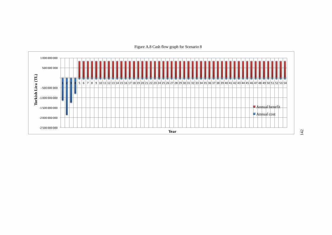
142
Figure A.8 Cash flow graph for Scenario 8
-2 500 000 000
-2 000 000 000
-1 500 000 000
-1 000 000 000
- 500 000 000
500 000 000
1 000 000 000
1 2 3 4 5 6 7 8 9 10 11 12 13 14 15 16 17 18 19 20 21 22 23 24 25 26 27 28 29 30 31 32 33 34 35 36 37 38 39 40 41 42 43 44 45 46 47 48 49 50 51 52 53 54
Tu
rk
ish
Lir
a (
TL
)
Year
Annual benefit
Annual cost
14
2
2

143
Table A.9 Internal rate of return for Scenario 9
Year Costs Benefits Net Benefit Net Present Value
1 1 132 731 429 -1 132 731 429 -1052 379 704
2 1 863 246 576 -1 863 246 576 -1494 193 596
3 1 240 857 607 -1 240 857 607 -858 913 665
4 789 986 723 - 789 986 723 -471 996 071
5 59 757 678 1089 271 354 1029 513 676 530 935 466
6 59 757 678 1089 271 354 1029 513 676 458 281 961
7 59 757 678 1089 271 354 1029 513 676 395 570 402
8 59 757 678 1089 271 354 1029 513 676 341 440 328
9 59 757 678 1089 271 354 1029 513 676 294 717 443
10 59 757 678 1089 271 354 1029 513 676 254 388 144
11 59 757 678 1089 271 354 1029 513 676 219 577 529
12 59 757 678 1089 271 354 1029 513 676 189 530 417
13 59 757 678 1089 271 354 1029 513 676 163 594 969
14 59 757 678 1089 271 354 1029 513 676 141 208 543
15 59 757 678 1089 271 354 1029 513 676 121 885 487
16 59 757 678 1089 271 354 1029 513 676 105 206 609
17 59 757 678 1089 271 354 1029 513 676 90 810 078
18 59 757 678 1089 271 354 1029 513 676 78 383 576
19 59 757 678 1089 271 354 1029 513 676 67 657 524
20 59 757 678 1089 271 354 1029 513 676 58 399 231
21 59 757 678 1089 271 354 1029 513 676 50 407 847
22 59 757 678 1089 271 354 1029 513 676 43 510 009
23 59 757 678 1089 271 354 1029 513 676 37 556 076
24 59 757 678 1089 271 354 1029 513 676 32 416 881
25 59 757 678 1089 271 354 1029 513 676 27 980 937
26 59 757 678 1089 271 354 1029 513 676 24 152 010
27 59 757 678 1089 271 354 1029 513 676 20 847 036
28 59 757 678 1089 271 354 1029 513 676 17 994 316
29 59 757 678 1089 271 354 1029 513 676 15 531 963
30 59 757 678 1089 271 354 1029 513 676 13 406 561
31 59 757 678 1089 271 354 1029 513 676 11 572 000
32 59 757 678 1089 271 354 1029 513 676 9 988 481
33 59 757 678 1089 271 354 1029 513 676 8 621 651
34 59 757 678 1089 271 354 1029 513 676 7 441 860
35 59 757 678 1089 271 354 1029 513 676 6 423 512
36 59 757 678 1089 271 354 1029 513 676 5 544 515
37 59 757 678 1089 271 354 1029 513 676 4 785 800
38 59 757 678 1089 271 354 1029 513 676 4 130 909
39 59 757 678 1089 271 354 1029 513 676 3 565 633
40 59 757 678 1089 271 354 1029 513 676 3 077 710
41 59 757 678 1089 271 354 1029 513 676 2 656 554
42 59 757 678 1089 271 354 1029 513 676 2 293 030
43 59 757 678 1089 271 354 1029 513 676 1 979 250
44 59 757 678 1089 271 354 1029 513 676 1 708 409
45 59 757 678 1089 271 354 1029 513 676 1 474 629
46 59 757 678 1089 271 354 1029 513 676 1 272 840
47 59 757 678 1089 271 354 1029 513 676 1 098 664
48 59 757 678 1089 271 354 1029 513 676 948 322
49 59 757 678 1089 271 354 1029 513 676 818 553
50 59 757 678 1089 271 354 1029 513 676 706 542
51 59 757 678 1089 271 354 1029 513 676 609 858
52 59 757 678 1089 271 354 1029 513 676 526 405
53 59 757 678 1089 271 354 1029 513 676 454 371
54 59 757 678 1089 271 354 1029 513 676 392 195
8 014 706 239 54 463 567 715 46 448 861 477 0
15.85%Internal Rate of Return :
Internal Rate of Return
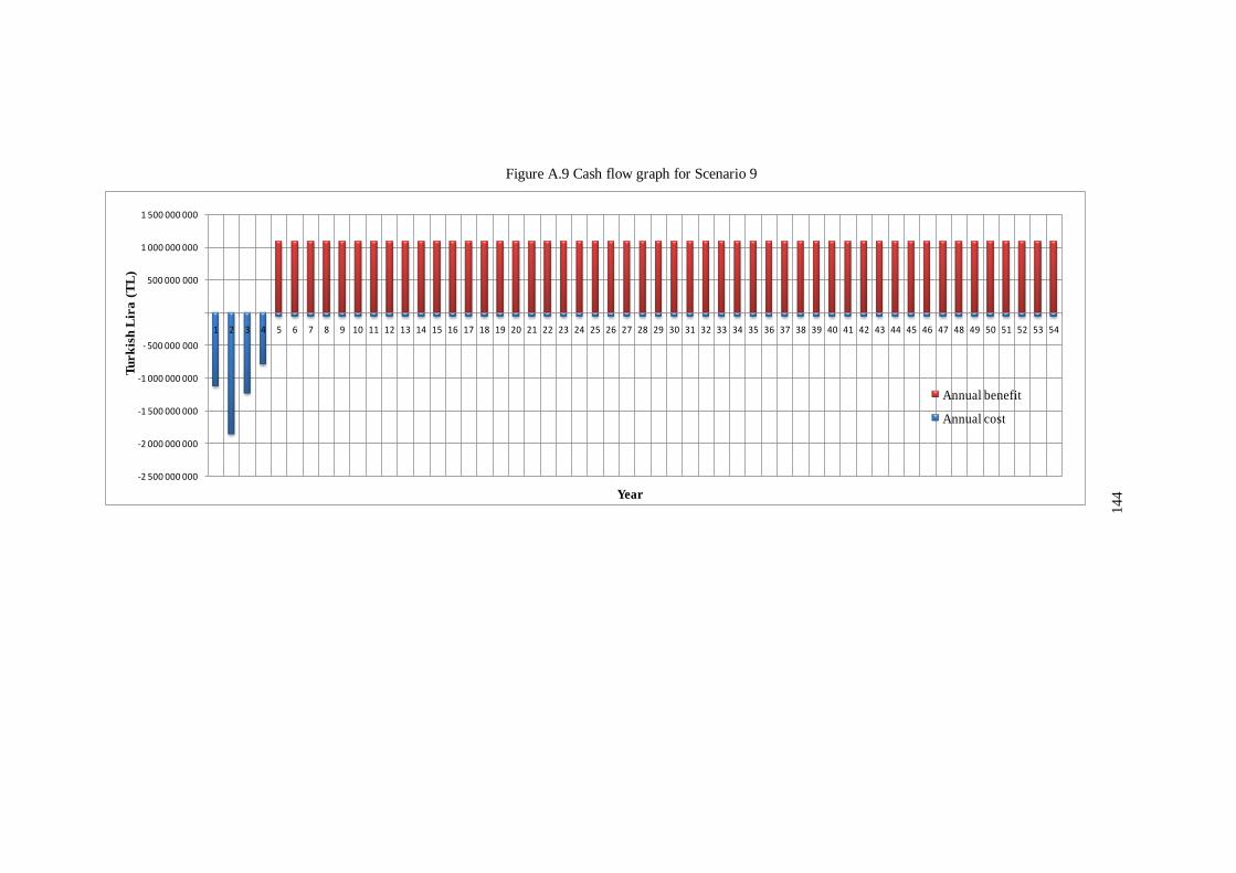
144
Figure A.9 Cash flow graph for Scenario 9
-2 500 000 000
-2 000 000 000
-1 500 000 000
-1 000 000 000
- 500 000 000
500 000 000
1 000 000 000
1 500 000 000
1 2 3 4 5 6 7 8 9 10 11 12 13 14 15 16 17 18 19 20 21 22 23 24 25 26 27 28 29 30 31 32 33 34 35 36 37 38 39 40 41 42 43 44 45 46 47 48 49 50 51 52 53 54
Tu
rk
ish
Lir
a (
TL
)
Year
Annual benefit
Annual cost
144
2

145
Table A.10 Internal rate of return for Scenario 10
Year Costs Benefits Net Benefit Net Present Value
1 1 150 188 429 -1 150 188 429 -1063 045 505
2 1 892 341 576 -1 892 341 576 -1493 991 460
3 1 275 771 607 -1 275 771 607 -860 373 923
4 824 900 723 - 824 900 723 -475 205 779
5 61 694 403 1215 365 043 1153 670 639 567 711 369
6 61 694 403 1215 365 043 1153 670 639 484 945 925
7 61 694 403 1215 365 043 1153 670 639 414 246 681
8 61 694 403 1215 365 043 1153 670 639 353 854 530
9 61 694 403 1215 365 043 1153 670 639 302 266 824
10 61 694 403 1215 365 043 1153 670 639 258 199 980
11 61 694 403 1215 365 043 1153 670 639 220 557 549
12 61 694 403 1215 365 043 1153 670 639 188 402 929
13 61 694 403 1215 365 043 1153 670 639 160 936 063
14 61 694 403 1215 365 043 1153 670 639 137 473 533
15 61 694 403 1215 365 043 1153 670 639 117 431 557
16 61 694 403 1215 365 043 1153 670 639 100 311 457
17 61 694 403 1215 365 043 1153 670 639 85 687 261
18 61 694 403 1215 365 043 1153 670 639 73 195 096
19 61 694 403 1215 365 043 1153 670 639 62 524 137
20 61 694 403 1215 365 043 1153 670 639 53 408 875
21 61 694 403 1215 365 043 1153 670 639 45 622 508
22 61 694 403 1215 365 043 1153 670 639 38 971 298
23 61 694 403 1215 365 043 1153 670 639 33 289 755
24 61 694 403 1215 365 043 1153 670 639 28 436 512
25 61 694 403 1215 365 043 1153 670 639 24 290 813
26 61 694 403 1215 365 043 1153 670 639 20 749 506
27 61 694 403 1215 365 043 1153 670 639 17 724 479
28 61 694 403 1215 365 043 1153 670 639 15 140 465
29 61 694 403 1215 365 043 1153 670 639 12 933 168
30 61 694 403 1215 365 043 1153 670 639 11 047 669
31 61 694 403 1215 365 043 1153 670 639 9 437 053
32 61 694 403 1215 365 043 1153 670 639 8 061 245
33 61 694 403 1215 365 043 1153 670 639 6 886 013
34 61 694 403 1215 365 043 1153 670 639 5 882 115
35 61 694 403 1215 365 043 1153 670 639 5 024 574
36 61 694 403 1215 365 043 1153 670 639 4 292 052
37 61 694 403 1215 365 043 1153 670 639 3 666 323
38 61 694 403 1215 365 043 1153 670 639 3 131 817
39 61 694 403 1215 365 043 1153 670 639 2 675 236
40 61 694 403 1215 365 043 1153 670 639 2 285 219
41 61 694 403 1215 365 043 1153 670 639 1 952 062
42 61 694 403 1215 365 043 1153 670 639 1 667 475
43 61 694 403 1215 365 043 1153 670 639 1 424 377
44 61 694 403 1215 365 043 1153 670 639 1 216 720
45 61 694 403 1215 365 043 1153 670 639 1 039 337
46 61 694 403 1215 365 043 1153 670 639 887 814
47 61 694 403 1215 365 043 1153 670 639 758 382
48 61 694 403 1215 365 043 1153 670 639 647 819
49 61 694 403 1215 365 043 1153 670 639 553 375
50 61 694 403 1215 365 043 1153 670 639 472 699
51 61 694 403 1215 365 043 1153 670 639 403 786
52 61 694 403 1215 365 043 1153 670 639 344 919
53 61 694 403 1215 365 043 1153 670 639 294 634
54 61 694 403 1215 365 043 1153 670 639 251 680
8 227 922 495 60 768 252 133 52 540 329 638 0
17.07%Internal Rate of Return :
Internal Rate of Return
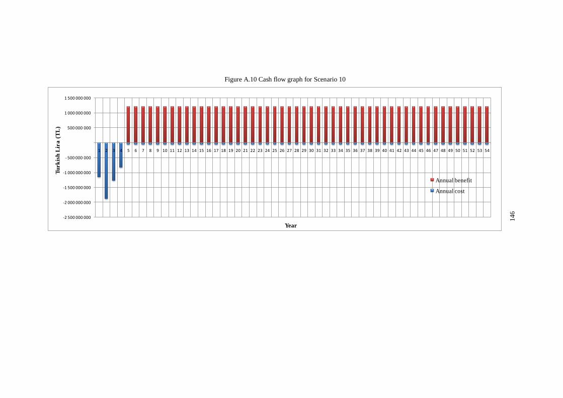
146
Figure A.10 Cash flow graph for Scenario 10
-2 500 000 000
-2 000 000 000
-1 500 000 000
-1 000 000 000
- 500 000 000
500 000 000
1 000 000 000
1 500 000 000
1 2 3 4 5 6 7 8 9 10 11 12 13 14 15 16 17 18 19 20 21 22 23 24 25 26 27 28 29 30 31 32 33 34 35 36 37 38 39 40 41 42 43 44 45 46 47 48 49 50 51 52 53 54
Tu
rk
ish
Lir
a (
TL
)
Year
Annual benefit
Annual cost
14
6
2

147
APPENDIX B
THE CHARACTERISTICS OF RESERVOIRS
Table B.1 The characteristics of Upper Kaleköy Dam
Dam Body
Type: roller compacted concrete (RCC)
Thalweg elevation: 1102.5 m
Foundation elevation: 1080.0 m
Crest elevation: 1230.0 m
Maximum operation water elevation: 1225.0 m
Minimum operation water elevation: 1210.0 m
Total volume of the reservoir: 595.3 hm³
Minimum volume of the reservoir: 406.2 hm³
Active volume: 189.1 hm³
Height from thalweg: 127.5 m
Height from foundation: 150.0 m
Spillway
Location: left bank
Design discharge: 8777 m³/s
Type: radial gated
Number of gates: 4
Crest elevation of spillway: 1209.5 m
Intake Structure and Penstocks
Invert elevation of intake structure: 1190.0 m
Number of penstocks: 3 + 1
Diameter of penstocks: 3 x 6.4 m + 1 x 2.2 m
Length of penstocks: 3 x 165.0 m + 1 x 169.0 m
Power Plant
Installed capacity: 600 MW (3 x 193.8 + 1 x18.6)
Tailwater level: 1102.5 m
Gross head: 122.5 m
Net head: 120.1 m

148
Figure B.1 General plan of Upper Kaleköy Dam and HEPP (Temelsu International Engineering Services Inc., 2011)
148
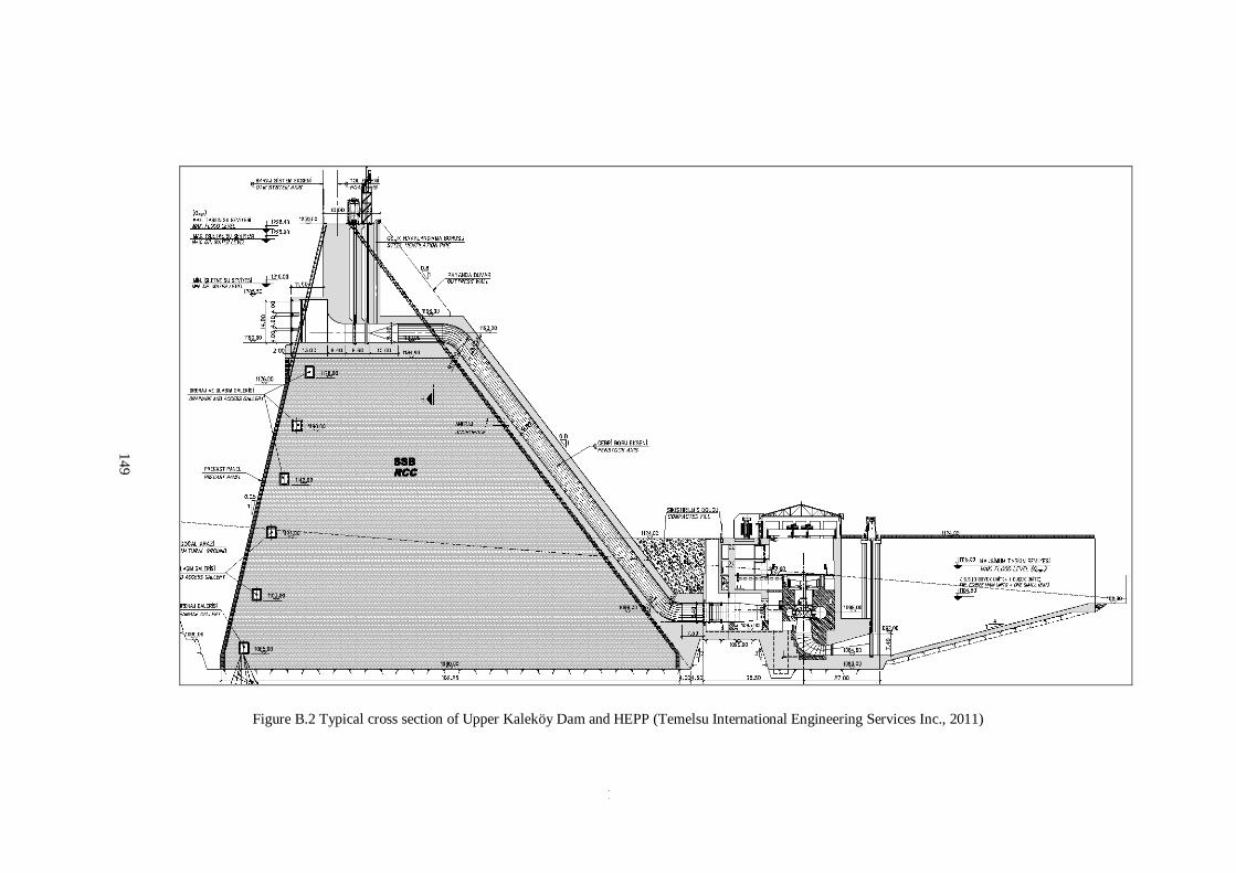
149
Figure B.2 Typical cross section of Upper Kaleköy Dam and HEPP (Temelsu International Engineering Services Inc., 2011)
14
9

150
Table B.2 The characteristics of Lower Kaleköy Dam
Dam Body
Type: roller compacted concrete (RCC)
Thalweg elevation: 1017.3 m
Foundation elevation: 1005.0 m
Crest elevation: 1107.5 m
Maximum operation water elevation: 1102.5 m
Minimum operation water elevation: 1085.0 m
Total volume of the reservoir: 431.5 hm³
Minimum volume of the reservoir: 240.1 hm³
Active volume: 191.4 hm³
Height from thalweg: 90.2 m
Height from foundation: 102.5 m
Spillway
Location: right bank
Design discharge: 9162 m³/s
Type: radial gated
Number of gates: 4
Crest elevation of spillway: 1087.0 m
Intake Structure and Penstocks
Invert elevation of intake structure: 1069.0 m
Number of penstocks: 3 + 1
Diameter of penstocks: 3 x 7.0 m + 1 x 2.4 m
Length of penstocks: 3 x 113.0 m + 1 x 117.0 m
Power Plant
Installed capacity: 450 MW
Tailwater level: 1020.0 m
Gross head: 82.5 m
Net head: 81.7 m

151
Figure B.3 General plan of Lower Kaleköy Dam and HEPP (Temelsu International Engineering Services Inc., 2011)
15
1

152
Figure B.4 Typical cross section of Lower Kaleköy Dam and HEPP (Temelsu International Engineering Services Inc., 2011)
15
2

153
Table B.3 The characteristics of Beyhan 1 Dam
Dam Body
Type: roller compacted concrete (RCC)
Thalweg elevation: 903.4 m
Foundation elevation: 890.0 m
Crest elevation: 987.0 m
Maximum operation water elevation: 982.0 m
Minimum operation water elevation: 977.0 m
Total volume of the reservoir: 369.06 hm³
Minimum volume of the reservoir: 294.64 hm³
Active volume: 74.42 hm³
Height from thalweg: 83.6 m
Height from foundation: 97.0 m
Spillway
Location: left bank
Design discharge : 10 528 m³/s
Type: radial gated
Number of gates : 6
Crest elevation of spillway: 967.0 m
Intake Structure and Penstocks
Invert elevation of intake structure at inlet: 962.0 m
Number of penstocks: 4
Diameter of penstock: 6.70 m / 4.80 m
Length of penstock: 4 x 10⁶ m
Power Plant
Installed capacity: 400 MW
Tailwater level: 905.0 m
Gross head: 77.0 m
Net head: 76.0 m

154
Figure B.5 General plan of Beyhan 1 Dam and HEPP (Temelsu International Engineering Services Inc., 2011)
15
4

155
Figure B.6 Typical cross section of Beyhan 1 Dam and HEPP (Temelsu International Engineering Services Inc., 2011)
15
5

156
Table B.4 The characteristics of Beyhan 2 Dam
Dam Body
Type : concrete gravity
Thalweg elevation : 868.2 m
Foundation elevation : 848.0 m
Crest elevation : 910.0 m
Maximum operation water elevation : 905.0 m
Minimum operation water elevation : 902.0 m
Total volume of the reservoir : 78.92 hm³
Minimum volume of the reservoir : 63.55 hm³
Active volume : 15.37 hm³
Height from thalweg : 41.8 m
Height from foundation : 62.0 m
Spillway
Location : on dam body
Design discharge : 10 528 m³/s
Type : radial gated
Number of gates : 6
Crest elevation of spillway : 890.0 m
Intake Structure and Penstocks
Invert elevation of intake structure at inlet : 875.0 m
Number of penstocks : 3 + 1
Diameter of penstocks : 3 x 7.8 m + 1 x 3.4 m
Length of penstocks : 3 x 76.0 m + 1 x 76.0 m
Power Plant
Installed capacity : 255 MW
Tailwater level : 870.0 m
Gross head : 35.0 m
Net head : 34.0 m

157
Figure B.7 General plan of Beyhan 2 Dam and HEPP (Temelsu International Engineering Services Inc., 2011)
15
7

158
Figure B.8 Typical cross section of Beyhan 2 Dam and HEPP (Temelsu International Engineering Services Inc., 2011)
15
8


![arXiv:2007.10937v1 [cs.CV] 21 Jul 2020Movie, where characters would face various situations and perform various behaviors in various scenarios, is a re ection of our real world. It](https://img.pdfslide.net/doc/110x75/60cf9bda5dbba423a638735b/arxiv200710937v1-cscv-21-jul-2020-movie-where-characters-would-face-various.jpg)