1

Operational Forecasting of Supercell Motion: Review and Case Studies Using Multiple Datasets

JON W. ZEITLER1

NOAA/National Weather Service Forecast Office, Austin/San Antonio, TX

MATTHEW J. BUNKERS

NOAA/National Weather Service Forecast Office, Rapid City, SD

(Submitted to National Weather Digest July 2004) (Revised December 2004)

(Final March 2005)

1* Corresponding author address: Mr. Jon W. Zeitler, Austin/San Antonio Weather

Forecast Office, 2090 Airport Road, New Braunfels, TX 78130.

E-mail: jon.zeitler@noaa.gov

2

ABSTRACT

The notion of anticipating supercell motion with multiple datasets in an operational

setting is addressed. In addition, the most common propagation mechanisms that regulate both

supercell and nonsupercell thunderstorm motion are reviewed. At minimum, supercell motion is

governed by advection from the mean wind and propagation via dynamic vertical pressure

effects. Therefore, one can use a hodograph to make predictions of supercell motion before

thunderstorms develop, or before thunderstorms split into right- and left-moving components.

This allows for better situational awareness and pathcasts of severe weather (relative to what

occurs without a priori knowledge of supercell motion), especially during the early stages of a

supercell’s lifetime. There are several potential sources of wind data readily available across the

United States, making it relatively easy to derive an ensemble of supercell motion estimates.

3

1. Introduction

Knowledge of supercell motion prior to thunderstorm formation is critical for successful

short-term forecasting of the associated severe weather, which in turn is fundamental for

emergency management and media preparations. For example, the forecast motion can be used

to determine the storm-relative helicity (SRH), as well as the storm-relative flow at the low,

middle, and upper levels of the supercell, which are important for evaluating tornadic potential

and precipitation distribution (e.g., Rasmussen and Straka 1998; Thompson 1998; Rasmussen

2003). Storm motion forecasts may also be useful in assessing convective mode (e.g., LaDue

1998; Bluestein and Weisman 2000). Moreover, a reasonable forecast of supercell motion—

relative to no knowledge of supercell motion—can lead to better pathcasts of hazardous weather

in severe local warnings, especially during the initial stages of the supercell’s lifetime (e.g., when

a thunderstorm is beginning to split into right- and left-moving supercells). This is important

since at least 90% of supercells are severe (e.g., Burgess and Lemon 1991) and most strong or

violent tornadoes are produced by supercells (e.g., Moller et al. 1994). In addition, Bunkers

(2002) found that 53 of 60 left-moving supercells produced severe hail (i.e., diameter ≥ 1.9 cm).

Modeling studies since the early 1980s (e.g., Weisman and Klemp 1986), field programs

such as Verifications of the Origins of Rotation in Tornadoes Experiment (VORTEX;

Rasmussen et al. 1994), and recent empirical studies (Bunkers et al. 2000; hereafter referred to as

B2K) indicate that supercell motion can be anticipated prior to, and monitored during, severe

weather operations. Despite the advances noted above, along with additional conference papers

(e.g., Bunkers and Zeitler 2000; Edwards et al. 2002) and computer-based training (UCAR

1999), routine use of the B2K supercell motion forecast technique (discussed in section 2g)

remains limited to a few entities within the operational forecasting community [e.g., the Storm

4

Prediction Center and a small percentage of the Weather Forecast Offices (WFOs)]. There may

be a number of reasons for the lack of use, including simple unawareness, incomplete or

inadequate training, lack of confidence in both the B2K technique and the general concept of

forecasting supercell motion, or perceived lack of real-time data for the determination of vertical

wind shear, supercell motion, and other derived parameters. The Sydney, NSW, Australia,

hailstorm of April 14, 1999 (Bureau of Meteorology 1999) illustrates the perils in not

understanding supercell processes, and motion deviant from the mean wind.

This study emphasizes the mechanisms that influence supercell motion, and addresses the

perceived lack of real-time data. A review of the most common mechanisms that control

supercell, and thunderstorm, motion is presented in section 2 to provide relevant background

information. Section 3 identifies near-real-time or real-time sources of wind profile data that can

be used to evaluate vertical wind shear and predict supercell motion. Section 4 contains four

case studies of supercell motion diagnosed or monitored by data sources listed in section 3.

Section 5 presents conclusions and recommended actions for operational forecasters.

2. Mechanisms controlling supercell motion

A discussion of the mechanisms that control supercell motion necessarily includes those

which affect the motion of nonsupercell thunderstorms. The two fundamental and distinctly

different physical controls on storm motion are (1) advection and (2) propagation—the latter of

which can be subdivided into several categories. In the current context, advection refers to the

movement of a convective element with the mean flow as it entrains horizontal momentum into

the updraft, whereas propagation refers to new convective initiation preferentially located

relative to existing convection such that it has an overall effect on storm motion (i.e., the

5

convection propagates through, not with, the mean flow). Propagation due to this new

convective development requires the three primary ingredients for deep moist convection:

moisture, instability, and upward motion. Based on a review of the literature, these two basic

controls (advection and propagation) can be delineated as follows:

(a) advection by the mean wind throughout a representative tropospheric layer,

(b) propagation via dynamic vertical pressure gradients due to a rotating updraft (germane to

supercells only),

(c) propagation via convective development along a thunderstorm’s outflow,

(d) propagation via convective development along a boundary layer convergence feature,

(e) propagation via storm mergers and interactions, and

(f) propagation via orographic effects such as upslope flow, lee-side convergence, and an

elevated heat source.

Other thunderstorm propagation mechanisms exist [e.g., propagation due to gravity waves;

Carbone et al. (2002)], but those listed above are believed to represent the most significant

influences on localized thunderstorm motion.

Storm motion is typically determined by tracking a prominent feature in radar reflectivity

or velocity data (e.g., the storm centroid, the mesocyclone, etc.). Tracking the storm centroid

gives the impression that a storm is an object, when in reality, the storm represents a process that

is strongly affected by parcel ascent (the growing part of the storm) and descent (the dissipating

part of the storm). Therefore, a storm continually changes due to these processes, and cannot be

considered a solid object (Hitschfeld 1960; Doswell 1985, p. 52). The propagation components

discussed in the present study largely represent storm processes of ascent.

6

Items (a) and (b) above are assumed to be the most important determinants of supercell

motion (see B2K and section 2g). The remaining four items (and especially d−f), while at times

very important, cannot be effectively anticipated with a hodograph on a consistent basis, and

instead must be inferred from observational data such as surface, satellite, radar, and topography.

However, it is noted that the general direction of (c) has potential predictability with a hodograph

based on the orientation of the low-level vertical wind shear vector (Rotunno et al. 1988).

Knowledge of these various thunderstorm/supercell propagation mechanisms (in addition to

advection) is especially important when attempting to make an accurate forecast of supercell

motion. Since there is still some disagreement regarding the processes that influence supercell

motion [e.g., see exchange by Klimowski and Bunkers (2002) and Weaver et al. (2002a,b)],

these mechanisms are discussed in the following paragraphs.

a) Advection

The most fundamental mechanism controlling the motion of deep moist convection is

advection by the mean wind throughout a representative tropospheric layer (e.g., Brooks 1946;

Byers and Braham 1949), which is analogous to (but not the same as) flow in a stream.

Hitschfeld (1960) described this process as conservation of horizontal momentum in rising or

descending parcels of air, which is tempered by entrainment. Utilizing radar data, these early

thunderstorm studies revealed the motion of discrete nonsupercell storms was highly correlated

with advection by the mean cloud-bearing wind [also see summary by Chappell (1986, pp. 293-

294)]. There have been many variations on what tropospheric layer is appropriate to calculate

the mean wind, but some commonly used methods have included the mandatory sounding levels

up to 300 or 200 hPa (e.g., Newton and Fankhauser 1964; Maddox 1976) or the layer from the

7

surface to 6 km (~20000 ft) (e.g., Byers and Braham 1949; Weisman and Klemp 1986; B2K)—

the top of which is often less than the maximum cloud height. In support of this shallower layer,

Wilhelmson and Klemp (1978) noted that the motion of modeled thunderstorms did not change

appreciably when the wind speeds above 6 km were substantially increased. By way of contrast,

Wilson and Megenhardt (1997) found that the 2-4 km layer gave the best results in predicting

convective cell motion in Florida. More recently, Ramsay and Doswell (2004) suggested a

deeper layer for advection of supercells (e.g., surface to 8 km). Obviously the “correct”

advection depth is dependent on factors such as the height of the storm (e.g., low-topped

supercells are advected over a shallower layer compared to tall storms), whether the storm’s

inflow is rooted in a near-surface layer or an elevated mixed layer (e.g., nocturnal convection

north of a warm front would not be affected by near-surface winds), or perhaps the storm’s age

(e.g., younger storms may be advected over a shallower layer relative to older storms).

Advection may also be regionally dependent, thus “scaling” the mean wind depth is potentially

useful (Thompson et al. 2004).

A frequently overlooked consideration in the calculation of the mean wind is whether or

not pressure-weighting (or similarly, density-weighting) is employed. Taking the average of the

mandatory pressure-level winds implicitly involves pressure-weighting because of the greater

concentration of mandatory levels in the lower half of a sounding. In this way, it is assumed that

advection dominates in the lower atmosphere—relative to the upper atmosphere—due to the

exponential decrease of pressure (density) with height. Pressure-weighting also has been used in

shallower atmospheric layers (e.g., Weisman and Klemp 1986), although it is unclear if this is

necessary based on the lack of statistical studies relating nonsupercell thunderstorm motion to

the mean wind. Clearly, this is an area that would benefit from additional research.

8

The effect of the mean wind on thunderstorm motion increases as the wind speed

increases. When the mean wind, and hence advection, is weak (< 10 m s-1), other propagation

mechanisms (described below) can have a significant impact on storm motion, but when the

mean wind is strong (> 20 m s-1), it tends to dominate over the propagation mechanisms. In the

absence of advection (i.e., the mean wind is near zero), the only other control on thunderstorm

motion is propagation. The most relevant propagation mechanisms are described throughout the

remainder of this section.

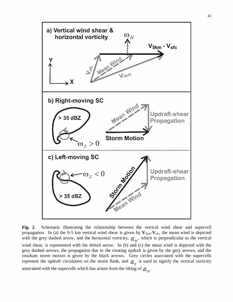
b) Shear-induced propagation

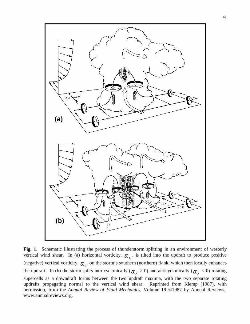
The feature that sets supercells apart from other thunderstorms is their persistent, rotating

updraft in the midlevels of the storm (Fig. 1; Doswell and Burgess 1993; Moller et al. 1994).

Although a multicellular structure can be imposed upon a supercell, a rotating updraft lasting at

least tens of minutes in the lower- to mid-levels of a thunderstorm defines it as a supercell. This

rotation results from the interaction of the updraft with the vertically sheared environment,

whereby low-level horizontal vorticity (ωH; Figs. 1a & 2a) is tilted into the vertical and

becomes spatially associated with the updraft (Figs. 1b & 2b,c). The rotating updraft, in turn,

produces a localized region of lowered pressure in the midlevels of the storm, which creates an

upward-directed pressure gradient force (Klemp 1987; Fig. 1). With respect to the three primary

ingredients for deep moist convection (i.e., moisture, instability, and upward motion), this

pressure gradient force provides enhanced upward motion on a preferred storm flank to initiate

new convective development. Numerical modeling studies have shown that this dynamic

interaction can contribute around 50% of the total updraft strength (Weisman and Rotunno 2000;

see their Fig. 13). This effect produces a horizontal updraft−shear propagation (USP) component

9

that is perpendicular to the shear vector and anti-parallel (parallel) to the horizontal vorticity

vector for the right-moving (left moving) supercell (Fig. 2b,c; also see Weisman and Klemp

1986). It is this basic attribute of supercells that largely explains the often disparate motion of

right- and left-moving supercells (Davies-Jones 2002).

Davies-Jones (2002) further subdivided the shear effects into linear and nonlinear

components. The nonlinear component is described above, and the linear component is a

function of hodograph curvature which is maximized for circular hodographs. It is beyond the

scope of this paper to discuss the details of these differences, but both effects lead to propagation

that is perpendicular to the shear vector.

In general, USP manifests itself through continuous (or perhaps quasi-continuous)

movement of a supercell (as opposed to discrete movement), although this is a function of the

temporal and spatial resolution of the radar data. This propagation may also depend on the

strength of the vertical wind shear [i.e., stronger shear may lead to a larger propagation

component (Bunkers and Zeitler 2000)]. Propagation due to this updraft−shear interaction

becomes increasingly important as the mean wind speed decreases, the vertical wind shear

increases, and also for atypical hodograph orientations (see B2K). When the USP opposes the

mean wind, slow-moving supercells can result.

c) Gust-front propagation

As a thunderstorm matures and develops precipitation, it produces a relatively cold

outflow at the surface (Fujita 1959). The leading edge of this outflow acts as a lifting

mechanism, providing enhanced upward motion relative to the existing storm. New convective

cells may form due to the convergence of moist and unstable air along the leading edge of this

10

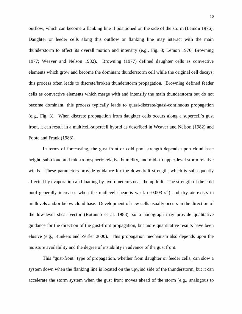
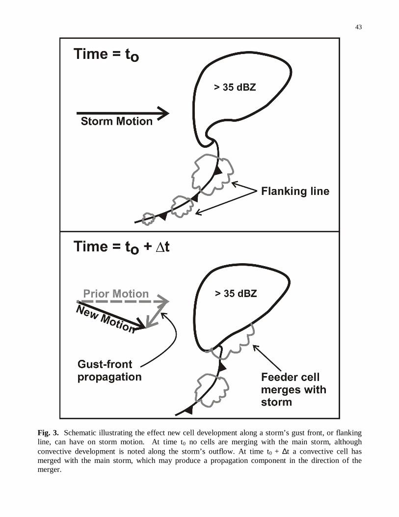
outflow, which can become a flanking line if positioned on the side of the storm (Lemon 1976).

Daughter or feeder cells along this outflow or flanking line may interact with the main

thunderstorm to affect its overall motion and intensity (e.g., Fig. 3; Lemon 1976; Browning

1977; Weaver and Nelson 1982). Browning (1977) defined daughter cells as convective

elements which grow and become the dominant thunderstorm cell while the original cell decays;

this process often leads to discrete/broken thunderstorm propagation. Browning defined feeder

cells as convective elements which merge with and intensify the main thunderstorm but do not

become dominant; this process typically leads to quasi-discrete/quasi-continuous propagation

(e.g., Fig. 3). When discrete propagation from daughter cells occurs along a supercell’s gust

front, it can result in a multicell-supercell hybrid as described in Weaver and Nelson (1982) and

Foote and Frank (1983).

In terms of forecasting, the gust front or cold pool strength depends upon cloud base

height, sub-cloud and mid-tropospheric relative humidity, and mid- to upper-level storm relative

winds. These parameters provide guidance for the downdraft strength, which is subsequently

affected by evaporation and loading by hydrometeors near the updraft. The strength of the cold

pool generally increases when the midlevel shear is weak (~0.003 s-1) and dry air exists in

midlevels and/or below cloud base. Development of new cells usually occurs in the direction of

the low-level shear vector (Rotunno et al. 1988), so a hodograph may provide qualitative

guidance for the direction of the gust-front propagation, but more quantitative results have been

elusive (e.g., Bunkers and Zeitler 2000). This propagation mechanism also depends upon the

moisture availability and the degree of instability in advance of the gust front.

This “gust-front” type of propagation, whether from daughter or feeder cells, can slow a

system down when the flanking line is located on the upwind side of the thunderstorm, but it can

accelerate the storm system when the gust front moves ahead of the storm [e.g., analogous to

11

Corfidi’s (2003) discussion of forward-propagating mesoscale convective systems (MCSs)]. It is

not known how often this phenomenon occurs with supercells, but Klemp (1987) noted that this

type of propagation may play a secondary role for supercells when compared to the USP

discussed in section 2b. Since low-precipitation (LP) supercells are less likely to have a

significant cold pool, relative to non-LP supercells, gust-front propagation is least likely with

these supercells.

d) Boundary layer convergence features

A common method of propagation for thunderstorm complexes is due to convective

development along boundary layer convergence features such as fronts, drylines, moisture/

instability axes, and outflow boundaries, which often leads to discrete thunderstorm propagation

(e.g., Newton and Fankhauser 1964; Weaver 1979; Magsig et al. 1998). This propagation

mechanism is not to be confused with gust-front propagation discussed in section 2c, although

the two are interrelated when a gust front is interacting with a boundary layer convergence zone.

This mechanism is driven by convergence of moist and unstable air that is often enhanced near

boundaries (e.g., Weaver 1979; Maddox et al. 1980), which results in an increased probability of

the initiation of deep moist convection (Wilson and Schreiber 1986). Furthermore, this process

is often aided by the transport of moist and unstable air in a low-level jet, especially for MCSs

(Corfidi et al. 1996).

Propagation due to boundary layer convergence features is different from (b) and (c)

above since the existing thunderstorm is not enhancing upward motion; rather, the enhanced

upward motion is derived from the convergence zone. Therefore, if a supercell is close enough

to a boundary layer convergence zone, it may preferentially “move” along or toward this feature

12

due to the development of new convective updrafts proximate to this favorable environment.

Moreover, supercells or multicell-supercell hybrid storms may propagate against the mean flow

in these low-level convergence zones due to mergers with daughter or feeder cells, resulting in

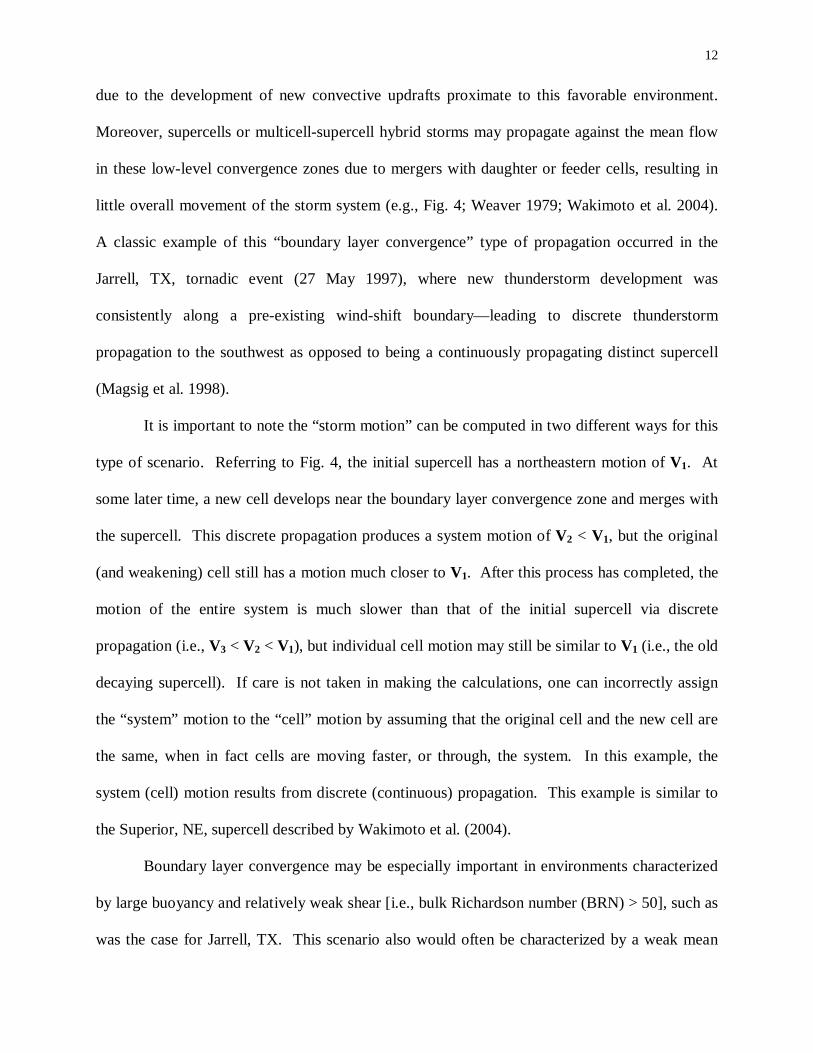
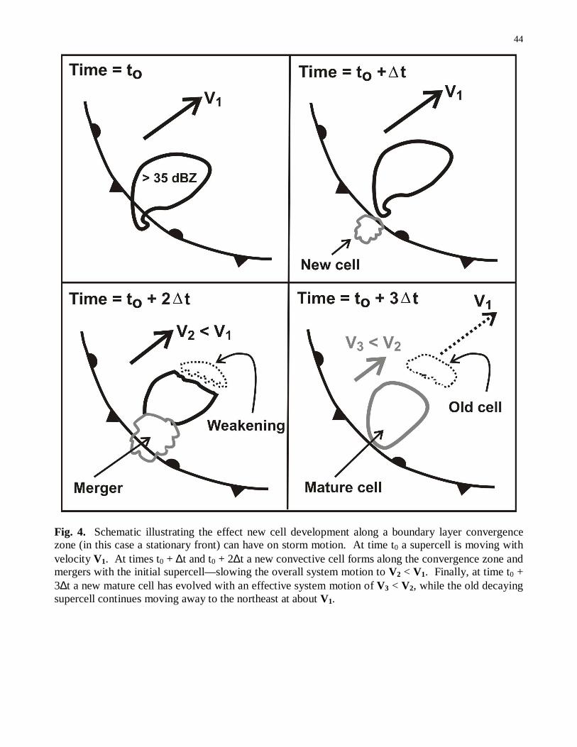
little overall movement of the storm system (e.g., Fig. 4; Weaver 1979; Wakimoto et al. 2004).

A classic example of this “boundary layer convergence” type of propagation occurred in the

Jarrell, TX, tornadic event (27 May 1997), where new thunderstorm development was

consistently along a pre-existing wind-shift boundary—leading to discrete thunderstorm

propagation to the southwest as opposed to being a continuously propagating distinct supercell

(Magsig et al. 1998).

It is important to note the “storm motion” can be computed in two different ways for this

type of scenario. Referring to Fig. 4, the initial supercell has a northeastern motion of V1. At

some later time, a new cell develops near the boundary layer convergence zone and merges with

the supercell. This discrete propagation produces a system motion of V2 < V1, but the original

(and weakening) cell still has a motion much closer to V1. After this process has completed, the

motion of the entire system is much slower than that of the initial supercell via discrete

propagation (i.e., V3 < V2 < V1), but individual cell motion may still be similar to V1 (i.e., the old

decaying supercell). If care is not taken in making the calculations, one can incorrectly assign

the “system” motion to the “cell” motion by assuming that the original cell and the new cell are

the same, when in fact cells are moving faster, or through, the system. In this example, the

system (cell) motion results from discrete (continuous) propagation. This example is similar to

the Superior, NE, supercell described by Wakimoto et al. (2004).

Boundary layer convergence may be especially important in environments characterized

by large buoyancy and relatively weak shear [i.e., bulk Richardson number (BRN) > 50], such as

was the case for Jarrell, TX. This scenario also would often be characterized by a weak mean

13

wind (< 10 m s-1), thus thunderstorms would be more likely to stay close to boundary layer

convergence zones for a longer period of time than when the mean wind is strong (> 20 m s-1).

Newton and Fankhauser (1964) attempted to explain the deviant motions (relative to the mean

wind) as being related to water-budget constraints, such that the largest storms—relative to the

small storms—moved farthest to the right of the mean wind, thereby “intercepting” a larger

volume of water vapor. Using a numerical cloud model, Atkins et al. (1999) studied the

interaction of simulated supercells with preexisting boundary layer convergence zones and found

that the effect on storm motion was about 5 m s-1. When propagation due to boundary layer

convergence dominates thunderstorm motion, locally heavy rainfall becomes increasingly likely.

e) Storm mergers and interactions

Very few studies have addressed the effects of storm mergers on subsequent storm

motion, although considerable anecdotal evidence exists for its occurrence. In general, this

occurs when there is an intersection of the paths of two thunderstorms whereby hydrometeors are

redistributed between the storms, and their updrafts and downdrafts interact. For example,

downdrafts may merge to initiate new convection via bridging (Westcott 1994), or the downdraft

from one storm may enhance the downdraft of another storm, causing it to accelerate. There are

times when storm mergers and interactions may lead to the intensification of existing convection

(Lemon 1976), but there are other times when convection may be affected negatively by a

merger (Westcott 1984). The effect of mergers on storm motion has not been investigated as

extensively as the effects of the other propagation mechanisms discussed herein. However, in a

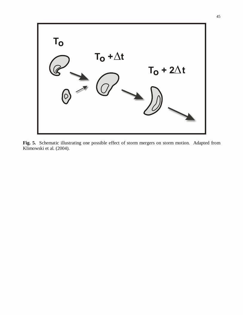
study of bow-echo evolution across the United States, Klimowski et al. (2004) showed that when

thunderstorms merge to become a bow echo, the subsequent motion of the bow echo was often

14

dictated by the most dominant and aggressive cell prior to merger, which was usually the cell

that initiated the merger (e.g., Fig. 5). This often resulted in an acceleration of the storm.

Cell mergers become increasingly likely when there are (1) numerous thunderstorms, (2)

differing storm motions, and (3) strong linear synoptic forcing. Thunderstorms are most

numerous when moisture, instability, and upward motion are relatively large, and convective

inhibition and vertical wind shear are relatively weak. Differing storm motions can occur for a

number of reasons: splitting thunderstorms and ordinary storms, short and tall storms being

advected by different atmospheric layers, and discrete propagation due to gust fronts, boundary

layer convergence features, and orography (discussed below). Finally, strong linear synoptic

forcing acts to concentrate thunderstorms along a common feature (e.g., front or dryline), which

then promotes adjacent cell interactions (e.g., Bluestein and Weisman 2000). Storm mergers can

also occur in conjunction with gust fronts (e.g., Fig. 3) and boundary layer convergence zones

(e.g., Fig. 4), making it difficult to separate the two mechanisms, and at times leading to an

“anchoring” of convection.

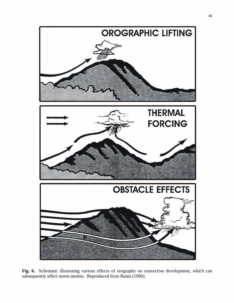
f) Orographic effects

Orography can also significantly influence supercell and nonsupercell thunderstorm

motion. Elevated terrain can provide enhanced mesoscale convergence zones in at least three

ways: (1) upslope flow, (2) lee-side convergence, and (3) an elevated heat source (Fig. 6; Kuo

and Orville 1973; Banta 1990). New cells may continually develop in these favored regions as

old ones advect away, leading to discrete thunderstorm propagation such that the system motion

is near zero—effectively “anchoring” the thunderstorm system to the elevated terrain (e.g.,

Akaeda et al. 1995). As a result, this effect is very similar to that of boundary layer convergence

15

zones discussed in section 2d, but the forcing mechanisms are clearly distinct. Nearby storms

that are not affected by mountainous terrain may have a substantial motion relative to those

being influenced by the orography. This effect appears to be most important when the mean

wind is relatively weak (< 10 m s-1) so that storms are not rapidly advected away from the source

of mesoscale convergence.

Orography can also have other effects on storms, such as causing their demise in a

downslope flow region or modulating their intensity by disrupting the inflow. Although this

does not affect storm motion directly, it does affect storm evolution, which is an important

forecast consideration.

g) Predicting supercell motion

B2K used 260 hodographs from supercell environments to develop a method to predict

supercell motion, and they also reviewed methods that were applicable to the prediction of

supercell motion. Their method assumes that advection and USP are the dominant mechanisms

controlling supercell motion [effects a−b above; Fig. 2]; these two effects can be easily

computed with a hodograph. [A tutorial on hodograph interpretation can be found in Doswell

(1991) and UCAR (2003).] Using a hodograph and the B2K method, supercell motion can be

predicted as follows (shown schematically in Fig. 7):

(1) plot a representative mean wind, which may be derived from the surface to 6 km (B2K),

the surface to 8 km (Ramsay and Doswell (2004), or a layer above the surface for

elevated supercells (e.g., Thompson et al. 2004);

(2) draw a shear vector that extends from the boundary layer (BL) to 5.5−6 km;

16

(3) draw a line that both passes through the mean wind and is orthogonal to the shear vector

(this represents the USP component; refer to section 2b); and

(4) plot the right-moving (left moving) supercell motion 7−8 m s-1 from the mean wind, and

along the orthogonal line to the right (left) of the shear vector.

In addition to plotting the forecast supercell motion on a hodograph, the B2K method can be

applied to numerical model data, and therefore storm motion vectors can be overlaid on radar

imagery, as is demonstrated in section 4c (also see Klimowski and Bunkers 2002).

There are times when several of the six items discussed above (advection plus five

propagation mechanisms) might play a role in supercell motion, and this reduces the

effectiveness of B2K’s technique. Moreover, poor supercell motion estimates—from any

method—may occur due to (1) use of an unrepresentative sounding, (2) use of an inappropriate

mean wind layer, and (3) varying deviations from the mean wind due to USP, which may be

dependent upon the strength of the vertical wind shear or to thermodynamic considerations.

However, B2K showed a 1−2 m s-1 improvement in mean absolute error over other methods

available to predict supercell motion (e.g., 30 degrees to the right of the mean wind and 70

percent of the mean wind speed). More recently, Edwards et al. (2002) and Ramsay and Doswell

(2004) found the B2K method to be statistically superior to other supercell motion forecasting

schemes, and Edwards et al. (2004) applied the B2K method to a dataset of 32 left-moving

supercells. Therefore, this technique will be used in section 4 to show how supercell motion can

be anticipated operationally.

3. Sources of wind information in the vertical

17

a) Radiosonde observations

A scan of WFO area forecast discussions (AFDs) shows that radiosonde observations

(RAOBs) are still the most popular source of data for tropospheric wind information. This is

understandable from the standpoint that RAOBs have been the traditional data source spanning

the advent of modern meteorology after World War II. In addition, RAOBs have the positive

attributes of (i) in-situ data, (ii) concurrent thermodynamic and wind data, and (iii) well-known

and minimized equipment and acquisition errors. Unfortunately, RAOBs have two substantial

limitations, especially with respect to forecasting and monitoring severe convection: (i) poor

spatial resolution [69 sites in the Continental United States (CONUS) (Peterson and Durre

2004)], and (ii) poor temporal resolution (observations typically at 12-h intervals). Many

individual storms, and even entire mesoscale convective systems (MCSs), can initiate, mature,

and dissipate without being sampled by the RAOB network. Forecasters attempt to remedy these

deficiencies by modifying RAOBs to represent the current or forecast (temporal), and/or nearby

(spatial) environment. Doswell (1991) discussed some of the pitfalls in these modifications, and

Brooks et al. (1994) discussed the notion of proximity soundings. Overall, RAOBs are the best

source of data if spatially and temporally near convection; however, in many instances this is not

the case.

b) 404 MHz vertical wind profilers

The NOAA Profiler Network (NPN; formerly Wind Profiler Demonstration Network)

provides a remotely sensed source of vertical wind information, primarily across the Great Plains

(NOAA 1994). The primary advantages of the NPN are high temporal resolution (averaged

18

observations at least hourly), and a vertical resolution of 250 m. These attributes are especially

useful when monitoring the low-level jet across the central United States during convective

situations. However, disadvantages of the NPN include only four sites outside the Great Plains

(three in Alaska, and one in central New York—the majority are between 30 and 45º N and 87

and 108º W), precipitation attenuation, and contamination from biologic sources such as bird

movements. NPN data have been found to be quantitatively consistent with the accuracy and

reliability of RAOBs (NOAA 1994). Further information on the NPN can be found at:

http://www.profiler.noaa.gov/jsp/index.jsp.

c) Doppler radar vertical wind profiles

The Weather Surveillance Radar-1988 Doppler (WSR-88D) vertical wind profiles

(VWPs) are a remotely sensed source of data with similar temporal resolution to the NPN. In

contrast to the NPN, the WSR-88D VWPs provide coverage across the CONUS, with the best

spatial resolution over the southern and eastern CONUS, and the poorest over the western

CONUS. VWP data are collocated with many CONUS RAOBs, which allows for comparison

studies near the 0000 UTC and 1200 UTC RAOB launches, but this collocation also reduces the

potential of sampling a larger geographical region if they were not collocated. The VWP data

share many of the same limitations as the NPN due to precipitation attenuation and biologic

contamination. Qualitatively, the VWP are of lesser quality than both RAOBs and the NPN

(Don Burgess, personal communication, 2003). An additional disadvantage of the WSR-88D

VWPs is the lack of data above the boundary layer prior to convection (due to a lack of

scatterers) (Klazura and Imy 1993; see their Table 1).

19

d) Aircraft Communication Addressing and Reporting System (ACARS)

Aircraft Communication Addressing and Reporting System (ACARS) observations

provide a growing source of wind profile data. The advantages of ACARS data include in-situ,

fast-response sensors, high vertical resolution, and on some aircraft, concurrent temperature and

dew point observations. Spatial and temporal resolution is good near hub airports (e.g., ATL,

DFW, LAX, MEM, ORD, SDF), but poor over the bulk of the CONUS except at altitudes above

7.5 km (~25,000 ft). However, new initiatives such as the Tropospheric Airborne

Meteorological Data Reporting System (TAMDAR; Daniels 2002) offer the prospects of much

higher spatial and temporal resolution below 7.5 km. Free data access is restricted to airlines,

NOAA, and research groups, thereby limiting the utility and applications of ACARS data.

Further details can be found at: http://acweb.fsl.noaa.gov.

e) Model analysis/forecast soundings

Another growing source of wind profile data are model analyses and forecasts. In fact,

many small operating units such as WFOs and universities regularly run local models allowing

for customization of resolution, domain, and physics. In general, model analyses are good,

especially for pre-convective environment. Studies by Thompson et al. (2003), and others (see

http://maps.fsl.noaa.gov), have shown fair to good agreement between model analysis profiles

and nearby RAOBs. Excellent horizontal, vertical, and temporal resolution can be tuned to

provide data in, or close, to the convective area of interest, reducing the time required to obtain a

“proximity” sounding dataset for studying tornadic vs. nontornadic supercells (e.g., Thompson et

20

al. 2003). However, disadvantages include errors introduced in the analysis or forecast process,

which can lead to errors in analysis or forecast fields.

f) Data sources summary

In general, observed data are preferred over model analyses or forecasts. Similarly, in-

situ data are preferred over remotely sensed observations, due to assumptions made in the remote

sensing retrieval process that may render misleading data. Finally, close temporal and spatial

proximity usually represents the near-storm environment better than observations further away.

Sometimes, a mix of the various data is required to obtain a reasonable estimate of the

environment in proximity to a given weather phenomenon (as the example in section 4a

illustrates). Table 1 provides a subjective summary of these data types.

4. Example cases

In the following four examples, knowledge of supercell motion outlined in section 2 is

used with the various datasets described in section 3 to show how supercell motion can be

effectively anticipated in an operational setting.

a) Southeast Texas—May 30, 1999

The Fort Bend County supercell of 30 May 1999 was one of several which formed as part

of a "northwest flow" event, referring to winds from 270 to 360 degrees at or above 3000 m in

response to an upper-level longwave ridge upstream and trough downstream of the convective

21

area (e.g., Johns 1982). These events have atypical hodographs as defined by B2K, resulting in

values of SRH and other storm-relative parameters to be unrepresentative of supercell potential

when the storm motion is estimated with non-Galilean invariant methods. [As noted in B2K,

Galilean invariant methods maintain the same storm motion forecast, relative to a given vertical

wind shear profile, no matter what the ground-relative wind profile looks like. However, non-

Galilean invariant methods can give different storm motion forecasts for the same vertical wind

shear profile but with differing ground-relative winds.] The supercell produced two reports of

1.9 cm hail, one F1 tornado (which destroyed a barn and numerous trees and power poles), and a

flash flood (“waist-deep” water in one subdivision). This was a relatively ordinary severe

weather episode, but is still useful to illustrate the concepts of forecasting supercell motion

operationally. It also highlights the importance of viewing supercell motion from the vertical

wind shear perspective (Galilean invariant), and not the mean wind perspective (non-Galilean

invariant).

Tracking the evolution and subsequent storm motion of the Fort Bend supercell was

complicated by convection along its flanking line, as well as a second storm to its southeast (Fig.

8). Although the Fort Bend supercell remained identifiable throughout its lifetime, the

convection along the flanking line periodically merged with the main storm (in the form of

feeder cells), and apparently accelerated it to the south-southwest (as discussed in the next

paragraph). Moreover, the second storm (Fig. 8) eventually merged with the Fort Bend supercell

on its downshear (eastern) flank, although its effect on storm motion is unclear. Finally, this

convection was occurring within a northeast−southwest axis of relatively moist and unstable air,

which may have further aided storm propagation through boundary layer convergence since the

storm-relative inflow was from the south-southwest. In summary, the Fort Bend supercell

22

appeared to be influenced by advection and four of the five supercell propagation mechanisms

discussed in section 2—orography being the only factor deemed unimportant.

The mean supercell motion for the Fort bend supercell was from 18 degrees at 7 m s-1.

Local forecaster vernacular for this type of movement is a "southwest-moving supercell"—

implying some special class of supercell. In reality, the supercell was moving to the right of the

mean shear vector. This motion is the same as a typical upper-right quadrant hodograph

supercell; except that the shear vector was rotated roughly 90 degrees clockwise from typical

orientations by the mean northwest flow. Figs. 9 through 12 show hodographs derived from four

different sources: (i) the 0000 UTC 5/31/1999 Corpus Christi (CRP), TX, RAOB, (ii) the 0000

UTC 5/31/1999 Lake Charles, LA, (LCH) RAOB, (iii) the 2300 UTC 5/30/1999 MAPS analysis

sounding nearest to Houston Hobby Airport (KHOU), and (iv) the 0014 UTC 5/31/1999

Houston/Galveston WSR-88D (KHGX) VWP. The 0000 UTC CRP hodograph produced the

smallest predicted motion error at 2.1 m s-1—although most of the data sources would have

provided a reasonable estimate of storm motion (i.e., 2−5 m s-1 errors), especially considering the

complicating factors of gust-front propagation and storm mergers. Non-Galilean invariant

methods, such as those based on a percentage of the mean wind speed and an angular deviation

to the right (e.g., 30R75), produce a supercell motion forecast to the east-southeast, and in error

by as much as 7−8 m s-1. In general, the supercell moved faster—to the south and west—than

predicted by the B2K method (e.g., Figs. 11 & 12). This is consistent with the merging feeder

cells observed along the southwestern leading edge of the storm (Fig. 8), which would accelerate

development along this flank of the supercell.

The values of 0-6 km total shear (Us), 0-6 km bulk shear (Ub), and 0-3 km SRH were

calculated for the wind profile sources listed above, plus three other plausible sources (Table 2).

Us was calculated by summing the shear segments across each 0.5-km sublayer from 0 to 6 km,

23

and Ub was calculated by determining the vector difference between the surface and 6-km winds.

Calculated Us ranged from 27.4 m s-1 to 48.9 m s-1, Ub ranged from 5.7 m s-1 to 21.6 m s-1, and

SRH ranged from 15 m2 s-2 to 220 m2 s-2. Us is greater than or equal to Ub by definition, since

hodograph curvature is neglected in the calculation of Ub.

Overall, Us was the least variable parameter (in terms of proportionality between the

largest to smallest values)—roughly 71%. Ub had a roughly 280% difference, which was due to

a wide variation in the 6-km wind. However, if the 0000 UTC LCH RAOB is discarded

(because of convective contamination in the mid-to-upper levels), and the 1200 UTC RAOBs are

omitted because of their temporal unrepresentativeness, then Ub (Us) only varied by 38% (71%).

SRH ranged an order of magnitude between largest and smallest, and when the smallest value of

SRH was omitted, the values still varied by 120%. These results agree with Markowski et al.

(1998), B2K, and Weisman and Rotunno (2000), that Us and Ub are more consistent predictors of

supercell potential than SRH (assuming initiation of deep moist convection).

Earlier points about the data sources are also evident. The 0014 UTC 5/31/99 KHGX

VWP was the closest non-model data source to the near-storm environment, and more strongly

indicated supercell potential than the other sources. The 2300 UTC 5/30/99 MAPS and RUC

analysis sounding statistics show that relatively small differences in Us (or Ub) can still be

associated with SRH differing by an order of magnitude between them (Table 2). [MAPS is the

development version of the RUC analysis/model run at the Forecast Systems Laboratory (FSL),

whereas the RUC is the operational version run at the National Centers for Environmental

Prediction (NCEP).] This example demonstrates that even minor changes to models can have

significant impacts for assessment of the near storm environment.

b) Central Texas—March 26, 2000

24

The central Texas supercells of March 26, 2000 were isolated left-moving (LM) and

right-moving (RM) components of a split from an initial thunderstorm near the Granger

(KGRK), TX, WSR-88D (Fig. 13). The LM supercell produced 2.2 to 6.9 cm hail, wind gusts to

31 m s-1, and wind damage to mobile homes and roofs. The RM supercell produced an F0

tornado four miles north of Seguin, TX, 4.4 to 6.3-cm hail, and widespread wind damage to

windows, roofs, cars, and power lines.

Fig. 14 shows the hodograph derived from the 0100 UTC 27 March 2000 MAPS analysis

sounding closest to KGRK. Unlike the Fort Bend supercell, these supercells were isolated, and

did not appear to be affected in a measurable way by gust-front propagation, boundary layer

convergence, storm mergers, or orography. Note the reasonable prediction of the motion of the

LM (V LM) and RM (VRM) supercells from the method of B2K—compared to the observed

supercell motions (Vobs) from 2223 UTC 26 March 2000 (shortly after the supercell split) to

0100 UTC 27 March 2000 (errors 1.9-2.4 m s-1). This case represents a situation where no

traditional wind data were readily available, but model analyses provided good insight into the

shear environment, resulting in a proper estimate of storm motions for the LM and RM

supercells.

This case also illustrates how situational awareness can be improved simply by

anticipating the motion of supercells, especially at far ranges from the radar in cases where data

may be limited or missing (e.g., Maddox et al. 2002; their Fig. 1). For example, if radar velocity

data were missing for this event, but the operational forecaster anticipated the tracks of the right-

and left-moving supercells, there would be a smaller chance of being surprised when the

supercells began to evolve, identification of supercells would be more straightforward, and

severe storm warnings could potentially be improved.

25

c) South-central South Dakota—August 3, 2001

On the afternoon of 3 August 2001, a single right-moving supercell (i.e., a thunderstorm

with a counterclockwise-rotating updraft) was observed over south central South Dakota. Severe

weather consisted of two hail reports (1.9 cm and 2.5 cm), and a wind gust to 27 m s-1. This

supercell was highly unusual in that it moved toward the northwest, and to the left of the mean

wind (discussed below). The synoptic setting contained a midlevel ridge with weak

northwesterly flow, but moderate southerly flow was prevalent in the lower atmosphere.

The initial thunderstorm formed around 1915 UTC, and supercell characteristics became

evident by 2000 UTC. The lifetime of this lone supercell thunderstorm (when it possessed

rotation) was about 90 minutes, and some mesocyclone alarms were indicated by the National

Severe Storms Laboratory (NSSL) mesocyclone detection algorithm (Stumpf et al. 1998). The

supercell moved northwest at 8 m s-1 (Fig. 15), and the parent thunderstorm dissipated by 2200

UTC.

The hodograph derived from the wind profiler at Merriman, NE, revealed that the

supercell moved to the left of the mean wind, but to the right of the vertical wind shear (Fig. 16).

Note that the B2K method had a storm motion error of 5.4 m s-1 (compare Vobs with VRM-fcst);

however, the B2K method provided useful guidance of the anomalous motion by indicating a

westward movement, which was to the right (left) of the shear vector (mean wind). This

information would greatly reduce the chance of being “surprised” by anomalous supercell

motion.

Referring back to the propagation mechanisms discussed in section 2, gust-front

propagation and boundary layer convergence were of similar importance in modulating storm

26

motion when compared to USP. First, the 0-6 km bulk shear was 13 m s-1, which is on the low

end for supercell occurrence [e.g., see Fig. 2 in Bunkers (2002)]. As a result, one might expect

USP not to be as significant as when the bulk shear is much stronger. Second, a sequence of

radar images revealed a gust front moving to the northwest, and away, from the supercell

thunderstorm. The gust front may have caused the supercell to accelerate toward the northwest

as the storm tried to “keep up” with this lifting mechanism. Indeed, the thunderstorm dissipated

after the gust front was 20 km ahead of it. Finally, the supercell occurred along a gradient of

moisture (Fig. 17), which might have been a source of enhanced instability. As noted in section

2d, this can lead to new convective development. In support of this, there was at least one period

of discrete propagation, toward the northwest, early in the supercell’s lifetime.

In summary, the supercell moved toward the northwest as a result of USP, gust-front

propagation, and boundary layer convergence. These latter two external forcing mechanisms can

become important when the wind shear is weak (as in this case). This unusual motion to the left

of the mean wind can be anticipated by viewing supercell motion from a vertical wind shear

perspective. Nearby wind profiler data were useful for assessing the vertical wind profile and

estimating storm motion. If a forecaster is utilizing the various datasets discussed in section 3 to

anticipate supercell motion before thunderstorms develop, they should not be caught off guard by

anomalous motion of supercells.

d) South-central South Dakota—June 30, 2003

During the late afternoon of June 30, 2003, ordinary thunderstorms over South Dakota

eventually gave way to one dominant long-lived supercell which lasted five hours. The supercell

initiated in south-central South Dakota, and traveled into north-central Nebraska before

27

dissipating. There were ten severe hail reports, ranging from 1.9−7.0 cm (five were from

golfball to baseball size). This event presented a warning challenge as storm motion changed

abruptly when the thunderstorm transitioned into a supercell, making the initial warning decision

difficult with respect to what area would be affected.

At 2247 UTC no severe storms or supercells were occurring in south-central South

Dakota, but ordinary nonsevere thunderstorms were moving east-northeast at 4-5 m s-1 (Fig.

18a). Between 2247 UTC and 2315 UTC, an ordinary storm rapidly developed into a supercell

and commenced moving southward at 4-5 m s-1 (Fig. 18b)—a change in direction of 100-120

degrees to the right. This change in direction was well forecast by the Rapid Update Cycle

(RUC) model using the B2K supercell motion forecasting method (Fig. 19a). As the supercell

traveled into Nebraska, it displayed a south-southwest motion, slightly farther to the right of the

motion indicated from the Merriman, NE, wind profiler (Fig. 19b).

In contrast to the previous example, the 0-6 km bulk shear was over twice as large in this

case (around 30 m s-1), suggesting a more significant USP component, which may explain the

stronger rightward deviation with time (Fig. 19a,b). None of the other propagation mechanisms

appeared to be playing a significant role in this case since discrete propagation was not evident,

no mergers occurred, and orography was not a factor.

In summary, this last case illustrates the usefulness of overlaying the mean wind and

supercell motion vectors on radar images when making warning decisions (also see Klimowski

and Bunkers 2002). The result can be improved short-term forecasts and warnings of severe

weather associated with supercells, especially during the initial stages of a supercell’s lifetime.

5. Conclusions and recommendations

28

Forecasting and monitoring supercell motion is critical to effective severe weather

operations. This understanding begins with a proper conceptual model of the factors that

influence supercell motion, which have been reviewed herein (refer to section 2). Armed with

this knowledge, operational forecasters can use all available datasets to anticipate supercell

motion. RAOBs are too spatially and temporally coarse to provide accurate wind profiles for

estimating supercell motion in over half of all events. Fortunately, NPN wind profiles, WSR-

88D VWPs, ACARS, and model analysis and forecast profiles can serve as surrogates for

improved estimates of the near-storm environment, resulting in better anticipation and forecasts

of supercell potential and motion. However, each source has advantages and disadvantages that

can render the acquired data either invaluable or nearly useless. The case studies from 30 May

1999, 26 March 2000, 3 August 2001, and 30 June 2003 are ordinary examples of how varied

data sources can provide differing levels of accuracy for anticipating supercells and forecasting

their motion.

The case studies presented herein only describe but a few ways in which supercell motion

can be anticipated operationally. In general, one starts with a baseline prediction using a

hodograph (or plan view display) and assumes advection and USP are dominant. This prediction

can then be modified contingent upon the anticipation of the other propagation mechanisms, if

they are deemed to be significant. Although prediction of supercell motion remains inexact,

clearly the potential exists to make substantial improvements in storm motion forecasts when

considering advection and the most common propagation mechanisms.

Despite the advances in supercell theory, observing systems, and operational modeling,

the severe weather operations meteorologist is still faced with applying a preponderance of

evidence in the selection of the most appropriate data source(s), especially for forecasts prior to

storm development. Knowledge of the mechanisms that control supercell motion, along with the

29

various data sources, parameter robustness, and preferred method for calculating storm motion,

will provide the best results for severe weather operations.

Acknowledgments. We thank Joe Arellano, Bill Read, and Dave Carpenter for supporting

this work, Steve Allen and Matt Moreland for assistance with data processing, and Dr. Joseph

Klemp for providing Fig. 1. Dr. John Knox, Michael Vescio, and Chris Smallcomb provided

valuable suggestions in the review process. Additionally, Drs. Andy Detwiler, Tom Fontaine,

Mark Hjelmfelt, Paul Smith, and Dennis Todey reviewed the manuscript, and Dr. Charles

Doswell III provided valuable insight on thunderstorm motion processes.

REFERENCES

Akaeda, K., J. Reisner, and D. Parsons, 1995: The role of mesoscale and topographically

induced circulations in initiating a flash flood observed during the TAMEX project. Mon.

Wea. Rev., 123, 1720-1739.

Atkins, N. T., M. L. Weisman, and L. J. Wicker, 1999: The influence of preexisting boundaries

on supercell evolution. Mon. Wea. Rev., 127, 2910-2927.

Banta, R. M., 1990: The role of mountain flows in making clouds. Atmospheric Processes Over

Complex Terrain, W. Blumen, Ed., Amer. Meteor. Soc., 229-283.

Bluestein, H. B., and M. L. Weisman, 2000: The interaction of numerically simulated supercells

initiated along lines. Mon. Wea. Rev., 128, 3128-3149.

Brooks, H. B., 1946: A summary of some radar thunderstorm observations. Bull. Amer. Meteor.

Soc., 27, 557-563.

Brooks, H. E., C. A. Doswell III, and J. Cooper, 1994: On the environments of tornadic and

nontornadic mesocyclones. Wea. Forecasting, 9, 606-618.

Browning, K. A., 1977: The structure and mechanisms of hailstorms. Hail: A Review of Hail

Science and Hail Suppression, Meteor. Monogr., No. 38, Amer. Meteor. Soc., 1-43.

30

Bunkers, M. J., 2002: Vertical wind shear associated with left-moving supercells. Wea.

Forecasting, 17, 845-855.

____, and J. W. Zeitler, 2000: On the nature of highly deviant supercell motion. Preprints, 20th

Conf. on Severe Local Storms, Orlando, FL, Amer. Meteor. Soc., 236-239.

____, B. A. Klimowski, J. W. Zeitler, R. L. Thompson, and M. L. Weisman, 2000: Predicting

supercell motion using a new hodograph technique. Wea. Forecasting, 15, 61-79.

Bureau of Meteorology, 1999: Report by the Director of Meteorology on the Bureau of

Meteorology's forecasting and warning performance for the Sydney hailstorm of 14 April

1999. Australian Bureau of Meteorology, Melbourne, Vic., Australia, 30 pp. Available at:

http://www.bom.gov.au/inside/services_policy/storms/sydney_hail/hail_report.shtml

Burgess, D. W., and L. R. Lemon, 1991: Characteristics of mesocyclones detected during a

NEXRAD test. Preprints, 25th Int. Conf. on Radar Meteorology, Paris, France, Amer. Meteor.

Soc., 39-42.

Byers, H. R., and R. R. Braham, 1949: The Thunderstorm. U.S. Government Printing Office,

Washington, DC, 287 pp.

Carbone, R. E., J. D. Tuttle, D. A. Ahijevych, and S. B. Trier, S. B.. 2002: Inferences of

predictability associated with warm season precipitation episodes. J. Atmos. Sci. 59, 2033–

2056.

Chappell, C. F., 1986: Quasi-stationary convective events. Mesoscale Meteorology and

Forecasting, P. S. Ray, Ed., Amer. Meteor. Soc., 289-310.

Corfidi, S. F., 2003: Cold pools and MCS propagation: Forecasting the motion of downwind-

developing MCSs. Wea. Forecasting, 18, 997-1017.

____, J. H. Merritt, and J. M. Fritsch, 1996: Predicting the movement of mesoscale convective

complexes. Wea. Forecasting, 11, 41-46.

Daniels, T.S., 2002: Tropospheric Airborne Meteorological Data Reporting System (TAMDAR)

sensor development. SAE General Aviation Technology Conference & Exhibition, Wichita,

KS. Available at: http://techreports.larc.nasa.gov/ltrs/PDF/2002/mtg/NASA-2002-saega-

tsd.pdf

Davies-Jones, R., 2002: Linear and nonlinear propagation of supercell storms. J. Atmos. Sci., 59,

3178-3205.

Doswell, C. A., III, 1985: The operational meteorology of convective weather. Vol. II: Storm

scale analysis. NOAA Tech. Memo. ERL ESG-15, NTIS PB85-226959, 240 pp.

31

____, 1991: A review for forecasters on the application of hodographs to forecasting severe

thunderstorms. Natl. Wea. Dig., 16, 2-16.

____, and D. W. Burgess, 1993: Tornadoes and tornadic storms: A review of conceptual

models. The Tornado: Its Structure, Dynamics, Prediction, and Hazards, Geophys. Monogr.,

No. 79, Amer. Geophys. Union, 161-172.

Edwards, R, R. L. Thompson, and J. A. Hart, 2002: Verification of supercell motion forecasting

techniques. Preprints, 21st Conf. on Severe Local Storms, San Antonio, TX, Amer. Meteor.

Soc., CD-ROM, J57-J60.

____, R. L. Thompson, and C. M. Mead, 2004: Assessment of anticyclonic supercell

environments using close proximity soundings from the RUC model. 22nd Conf. on Severe

Local Storms, Hyannis, MA, Amer. Meteor. Soc., CD-ROM, P1.2.

Foote, G. B., and H. W. Frank, 1983: Case study of a hailstorm in Colorado. Part III: Airflow

from triple-Doppler measurements. J. Atmos. Sci., 40, 686-707.

Fujita, T. T. 1959: Precipitation and cold air production in mesoscale thunderstorm systems.

J. Atmos. Sci., 16, 454–466.

Hitschfeld, W., 1960: The motion and erosion of convective storms in severe vertical wind

shear. J. Meteor., 17, 270-282.

Johns, R. H., 1982: A synoptic climatology of northwest flow severe weather outbreaks. Part I:

Nature and significance. Mon. Wea. Rev., 110, 1653-1663.

Klazura, G. E., and D. A. Imy, 1993: A description of the initial set of analysis products

available from the NEXRAD WSR-88D system. Bull. Amer. Meteor. Soc., 74, 1293-1311.

Klemp, J. B., 1987: Dynamics of tornadic thunderstorms. Ann. Rev. Fluid Mech., 19, 369-402.

Klimowski, B. A., and M. J. Bunkers, 2002: Comments on “Satellite Observations of a Severe

Supercell Thunderstorm on 24 July 2000 Made during the GOES-11 Science Test.” Wea.

Forecasting, 17, 1111-1117.

Klimowski, B. A., M. R. Hjelmfelt, and M. J. Bunkers, 2004: Radar observations of the early

evolution of bow echoes. Wea. Forecasting, 19, in press.

Kuo, J-T., and H. D. Orville, 1973: A radar climatology of summertime convective clouds in the

Black Hills. J. Appl. Meteor., 12, 359-368.

LaDue, J. G., 1998: The influence of two cold fronts on storm morphology. Preprints, 19th Conf.

On Severe Local Storms, Minneapolis, MN, Amer. Meteor. Soc., 324-327.

32

Lemon, L. R., 1976: The flanking line, a severe thunderstorm intensification source. J. Atmos.

Sci., 33, 686-694.

Maddox, R. A., 1976: An evaluation of tornado proximity wind and stability data. Mon. Wea.

Rev., 104, 133-142.

____, L. R. Hoxit, and C. F. Chappell, 1980: A study of tornadic thunderstorm interactions with

thermal boundaries. Mon. Wea. Rev., 108, 322-336.

____, J. Zhang, J. J. Gourley, and K. W. Howard, 2002: Weather radar coverage over the

contiguous United States. Wea. Forecasting, 17, 927–934.

Magsig, M. A., D. W. Burgess, and R. R. Lee, 1998: Multiple boundary evolution and

Tornadogenesis associated with the Jarrell Texas events. Preprints, 19th Conf. on Severe

Local Storms, Minneapolis, MN, Amer. Meteor. Soc., 186-189.

Markowski, P. M., J. M. Straka, E. N. Rasmussen, and D. O. Blanchard, 1998: Variability of

storm-relative helicity during VORTEX. Mon. Wea. Rev., 126, 2959-2971.

Moller, A. R., C. A. Doswell III, M. P. Foster, and G. R. Woodall, 1994: The operational

recognition of supercell thunderstorm environments and storm structures. Wea. Forecasting,

9, 327-347.

Newton, C. W., and J. C. Fankhauser, 1964: On the movements of convective storms, with

emphasis on size discrimination in relation to water-budget requirements. J. Appl. Meteor., 3,

651-668.

NOAA, 1994: Wind Profiler Assessment Report and Recommendations for Future Use. U.S.

Dept. of Commerce, National Oceanic and Atmospheric Administration, 141 pp.

Peterson, T. C., and I. Durre, 2004: A climate continuity strategy for the radiosonde replacement

system transition. Preprints, 8th Symp. on Integrated Observing and Assimilation Systems for

Atmosphere, Oceans, and Land Surface, Seattle, WA, Amer. Meteor. Soc., CD-ROM, 4.6B

Priegnitz, D. L., 1995: IRAS: Software to display and analyze WSR-88D radar data. Preprints,

11th International Conference on Interactive Information and Processing Systems (IIPS),

Boston, MA, Amer. Meteor. Soc., 197-199. Available at:

http://www.ncdc.noaa.gov/oa/radar/iras.html

Ramsay, H. A., and C. A. Doswell III, 2004: Exploring hodograph-based techniques to estimate

the velocity of right-moving supercells. 22nd Conf. on Severe Local Storms, Hyannis, MA,

Amer. Meteor. Soc., CD-ROM, 11A.6.

33

Rasmussen, E. N., 2003: Refined supercell and tornado forecast parameters. Wea. Forecasting,

18, 530-535.

____, and J. M. Straka, 1998: Variations in supercell morphology. Part I: Observations of the

role of upper-level storm-relative flow. Mon. Wea. Rev., 126, 2406-2421.

____, ____, R. Davies-Jones, C. A. Doswell III, F. H. Carr, M. D. Eilts, and D. R. MacGorman,

1994: Verifications of the Origins of Rotation in Tornadoes Experiment: VORTEX. Bull.

Amer. Meteor. Soc., 75, 995-1006.

Rotunno, R., J. B. Klemp, and M. L. Weisman, 1988: A theory for strong, long-lived squall

lines. J. Atmos. Sci., 45, 463-485.

Stumpf, G. J., A. Witt, E. D. Mitchell, P. L. Spencer, J. T. Johnson, M. D. Eilts, K. W. Thomas,

and D. W. Burgess, 1998: The National Severe Storms Laboratory mesocyclone detection

algorithm for the WSR-88D. Wea. Forecasting, 13, 304–326.

Thompson, R. L., 1998: Eta model storm-relative winds associated with tornadic and

nontornadic supercells. Wea. Forecasting, 13, 125-137.

____, C. M. Mead, and R. Edwards, 2004: Effective bulk shear in supercell thunderstorm

environments. 22nd Conf. on Severe Local Storms, Hyannis, MA, Amer. Meteor. Soc., CD-

ROM, P1.1.

____, R. Edwards, J. A. Hart, K. L. Elmore, and P. Markowski, 2003: Close proximity

soundings within supercell environments obtained from the Rapid Update Cycle. Wea.

Forecasting, 18, 1243-1261.

UCAR, 1999: Predicting Supercell Motion Using Hodograph Techniques. University

Corporation for Atmospheric Research, Cooperative Program for Operational Meteorology,

Education, and Training (COMET), Webcast. Available at:

http://meted.ucar.edu/convectn/ic411/]

____, 2003: Principles of Convection II: Using Hodographs. University Corporation for

Atmospheric Research, Cooperative Program for Operational Meteorology, Education, and

Training (COMET), Webcast. Available at: http://meted.ucar.edu/mesoprim/hodograf/

Wakimoto, R. M., H. Cai, and H. V. Murphey, 2004: The Superior, Nebraska, supercell during

BAMEX. Bull. Amer. Meteor. Soc., 85, 1095-1106.

Weaver, J. F., 1979: Storm motion as related to boundary-layer convergence. Mon. Wea. Rev.,

107, 612-619.

34

____, and S. P. Nelson, 1982: Multiscale aspects of thunderstorm gust fronts and their effects on

subsequent storm development. Mon. Wea. Rev., 110, 707-718.

____, J. A. Knaff, D. Bikos, G. S. Wade, and J. M. Daniels, 2002a: Satellite observations of a

severe supercell thunderstorm on 24 July 2000 made during the GOES-11 science test. Wea.

Forecasting, 17, 124-138.

____, ____, ____, ____, and ____, 2002b: Reply. Wea. Forecasting, 17, 1118-1127.

Weisman, M. L., and J. B. Klemp, 1986: Characteristics of isolated convective storms.

Mesoscale Meteorology and Forecasting, P. S. Ray, Ed., Amer. Meteor. Soc., 331-358.

____, and R. Rotunno, 2000: The use of vertical wind shear versus helicity in interpreting

supercell dynamics. J. Atmos. Sci., 57, 1452–1472.

Westcott, N., 1984: A historical perspective on cloud mergers. Bull. Amer. Meteor. Soc., 65,

219–227.

____, 1994: Merging of convective clouds: Cloud initiation, bridging, and subsequent growth.

Mon. Wea. Rev., 122, 780-790.

Wilhelmson, R. B., and J. B. Klemp, 1978: A numerical study of storm splitting that leads to

long-lived storms. J. Atmos. Sci., 35, 1974-1986.

Wilson, J. W., and D. L. Megenhardt, 1997: Thunderstorm initiation, organization, and lifetime

associated with Florida boundary layer convergence lines. Mon. Wea. Rev., 125, 1507–1525.

____, and W. E. Schreiber, 1986: Initiation of convective storms at radar-observed boundary-

layer convergence lines. Mon. Wea. Rev., 114, 2516-2536.

35

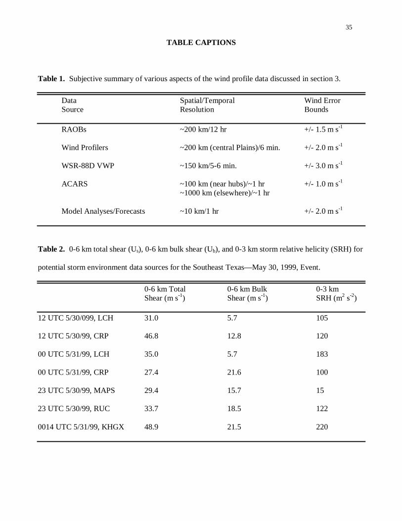
TABLE CAPTIONS

Table 1. Subjective summary of various aspects of the wind profile data discussed in section 3.

Data Spatial/Temporal Wind Error Source Resolution Bounds

RAOBs ~200 km/12 hr +/- 1.5 m s-1

Wind Profilers ~200 km (central Plains)/6 min. +/- 2.0 m s-1

WSR-88D VWP ~150 km/5-6 min. +/- 3.0 m s-1

ACARS ~100 km (near hubs)/~1 hr +/- 1.0 m s-1 ~1000 km (elsewhere)/~1 hr

Model Analyses/Forecasts ~10 km/1 hr +/- 2.0 m s-1

Table 2. 0-6 km total shear (Us), 0-6 km bulk shear (Ub), and 0-3 km storm relative helicity (SRH) for

potential storm environment data sources for the Southeast Texas—May 30, 1999, Event.

0-6 km Total 0-6 km Bulk 0-3 km Shear (m s-1) Shear (m s-1) SRH (m2 s-2)

12 UTC 5/30/099, LCH 31.0 5.7 105

12 UTC 5/30/99, CRP 46.8 12.8 120

00 UTC 5/31/99, LCH 35.0 5.7 183

00 UTC 5/31/99, CRP 27.4 21.6 100

23 UTC 5/30/99, MAPS 29.4 15.7 15

23 UTC 5/30/99, RUC 33.7 18.5 122

0014 UTC 5/31/99, KHGX 48.9 21.5 220

36

FIGURE CAPTIONS

Fig. 1. Schematic illustrating the process of thunderstorm splitting in an environment of westerly

vertical wind shear. In (a) horizontal vorticity, ωH, is tilted into the updraft to produce positive

(negative) vertical vorticity, ωZ, on the storm’s southern (northern) flank, which then locally enhances

the updraft. In (b) the storm splits into cyclonically (ωZ > 0) and anticyclonically (ωZ

< 0) rotating

supercells as a downdraft forms between the two updraft maxima, with the two separate rotating

updrafts propagating normal to the vertical wind shear. Reprinted from Klemp (1987), with

permission, from the Annual Review of Fluid Mechanics, Volume 19 ©1987 by Annual Reviews,

www.annualreviews.org.

Fig. 2. Schematic illustrating the relationship between the vertical wind shear and supercell

propagation. In (a) the 0-5 km vertical wind shear is given by V5km-Vsfc, the mean wind is depicted

with the grey dashed arrow, and the horizontal vorticity, ωH, which is perpendicular to the vertical

wind shear, is represented with the dotted arrow. In (b) and (c) the mean wind is depicted with the

grey dashed arrows, the propagation due to the rotating updraft is given by the grey arrows, and the

resultant storm motion is given by the black arrows. Grey circles associated with the supercells

represent the updraft circulation on the storm flank, and ωZ is used to signify the vertical vorticity

associated with the supercells which has arisen from the tilting of ωH.

Fig. 3. Schematic illustrating the effect new cell development along a storm’s gust front, or flanking

line, can have on storm motion. At time t0 no cells are merging with the main storm, although

convective development is noted along the storm’s outflow. At time t0 + ∆t a convective cell has

37

merged with the main storm, which may produce a propagation component in the direction of the

merger.

Fig. 4. Schematic illustrating the effect new cell development along a boundary layer convergence

zone (in this case a stationary front) can have on storm motion. At time t0 a supercell is moving with

velocity V1. At times t0 + ∆t and t0 + 2∆t a new convective cell forms along the convergence zone and

mergers with the initial supercell—slowing the overall system motion to V2 < V1. Finally, at time t0 +

3∆t a new mature cell has evolved with an effective system motion of V3 < V2, while the old decaying

supercell continues moving away to the northeast at about V1.

Fig. 5. Schematic illustrating one possible effect of storm mergers on storm motion. Adapted from

Klimowski et al. (2004).

Fig. 6. Schematic illustrating various effects of orography on convective development, which can

subsequently affect storm motion. Reproduced from Banta (1990).

Fig. 7. Schematic illustrating the steps in plotting the predicted supercell motion using a hodograph

and the method from Bunkers et al. (2000), which is discussed in section 2g.

Fig. 8. KHGX WSR-88D 0.5º reflectivity image at 2159 UTC 30 May 1999. The Fort Bend supercell

is discussed in section 4a. The Java-IRAS software was used to display the radar data (Priegnitz

1995).

38

Fig. 9. The 0000 UTC 31 May 1999 CRP RAOB hodograph. VRM-fcst is predicted right-moving

supercell motion from the method in Bunkers et al. (2000). VLM-fcst is the predicted left-moving

supercell motion. VOBS is the observed supercell motion. The dashed line represents the surface to 6

km shear. The square is the surface to 6 km mean wind. The asterisk is forecast storm motion based on

30° to the right of the mean wind direction and 70% of the mean wind speed. Units are m s-1.

Fig. 10. Same as Fig. 9, except for the 0000 UTC 31 May 1999 LCH RAOB hodograph.

Fig. 11. Same as Fig. 9, except for the 2300 UTC 30 May 1999 MAPS (KHOU) hodograph.

Fig. 12. Same as Fig. 9, except for the 0014 UTC 31 May 1999 KHGX VWP hodograph.

Fig. 13. Map of left-moving (LM) and right-moving (RM) storm locations and paths from 2303 UTC

26 March 2000 to 0110 UTC 27 March 2000. KAUS is Austin-Bergstrom International Airport;

KCLL is Easterwood Field-College Station; KHGX is the Houston/Galveston WSR-88D radar; KSAT

is San Antonio International Airport. The Java-IRAS software was used to display the radar data

(Priegnitz 1995).

Fig. 14. The 0100 UTC 3/27/2000 MAPS (KGRK) hodograph, VRM-fcst is predicted right-moving

supercell motion from the method in Bunkers et al. (2000). VLM-fcst is the predicted left-moving

supercell motion. VOBS are the observed right-moving and left-moving supercell motion. The dashed

line represents the surface to 6 km shear. The square is the surface to 6 km mean wind. Units are m s-1.

39

Fig. 15. KUDX WSR-88D 1.5º reflectivity composite for 2000 UTC and 2100 UTC 3 August 2001.

The storm location at 2000 UTC corresponds to the satellite image in Fig. 17. The Java-IRAS

software was used to display the radar data (Priegnitz 1995).

Fig. 16. Same as Fig. 9, except for the 2000-2200 UTC 3 August 2001 Merriman, NE, profiler

hodograph.

Fig. 17. Visible satellite image at 2000 UTC 3 August 2001. Surface observations are overlaid in

black, and subjectively drawn isodrosotherms are given for 60, 65, 70, and 75° F. For reference, the

Black Hills are located in the center of the left-hand side of the image.

Fig. 18. KUDX WSR-88D 0.5º reflectivity image at (a) 2247 UTC 30 June 2003 and (b) 2356 UTC

30 June 2003. Reflectivity shading corresponds to that in Fig. 15. The observed storm motion for the

previous 45-min period is displayed with respect to the direction the storm is traveling (knots).

Surface observations are overlaid in black. The 0-6 km mean wind vectors (knots) from the RUC

model are plotted on (a). The predicted supercell motion vectors from the RUC model using the

method from Bunkers et al. (2000) are plotted on (b).

Fig. 19. Same as Fig. 14, except for (a) the 0000 UTC 1 July 2003 RUC hodograph and (b) the 0100

UTC 1 July 2003 Merriman, NE, profiler hodograph.

40

AUTHORS PAGE

Jon W. Zeitler is the Science and Operations Officer at WFO Austin/San Antonio, TX. He previously

served as a Senior Forecaster at WFO Houston/Galveston, TX; a General Forecaster at WFO Rapid

City, SD; and as an Agricultural Weather Forecaster at the Southwest Agricultural Weather Service

Center (AWSC), College Station, TX. Prior to his NWS career, he was the Regional Climatologist at

the Southeast Regional Climate Center, Columbia, SC, and Assistant State Climatologist for Texas at

Texas A&M University, College Station, TX. He received a B.S. in meteorology from Iowa State

University in 1988, and a M.S. in meteorology from Texas A&M University in 1991. Jon’s interests

include mesoscale meteorology, severe convective storms, flash flood safety, statistics, and leadership

development.

Matthew J. Bunkers is the Science and Operations Officer at WFO Rapid City, SD. He previously

served in positions of Student Trainee, Meteorological Intern, General Forecaster, and Senior

Forecaster at WFO Rapid City. He received a B.S. in Interdisciplinary Sciences from the South

Dakota School of Mines & Technology (SDSM&T) in 1992, and a M.S. in Atmospheric Sciences from

SDSM&T in 1993. He is currently pursuing a Ph.D. in Atmospheric, Environmental, and Water

Resources at SDSM&T. Matt’s interests include severe convective storms, weather analysis &

forecasting, climatology, and statistics.

41

Fig. 1. Schematic illustrating the process of thunderstorm splitting in an environment of westerly vertical wind shear. In (a) horizontal vorticity, ωH

, is tilted into the updraft to produce positive

(negative) vertical vorticity, ωZ, on the storm’s southern (northern) flank, which then locally enhances

the updraft. In (b) the storm splits into cyclonically (ωZ > 0) and anticyclonically (ωZ

< 0) rotating

supercells as a downdraft forms between the two updraft maxima, with the two separate rotating updrafts propagating normal to the vertical wind shear. Reprinted from Klemp (1987), with permission, from the Annual Review of Fluid Mechanics, Volume 19 ©1987 by Annual Reviews, www.annualreviews.org.

42

Fig. 2. Schematic illustrating the relationship between the vertical wind shear and supercell propagation. In (a) the 0-5 km vertical wind shear is given by V5km-Vsfc, the mean wind is depicted with the grey dashed arrow, and the horizontal vorticity, ωH

, which is perpendicular to the vertical

wind shear, is represented with the dotted arrow. In (b) and (c) the mean wind is depicted with the grey dashed arrows, the propagation due to the rotating updraft is given by the grey arrows, and the resultant storm motion is given by the black arrows. Grey circles associated with the supercells represent the updraft circulation on the storm flank, and ωZ

is used to signify the vertical vorticity

associated with the supercells which has arisen from the tilting of ωH.

43

Fig. 3. Schematic illustrating the effect new cell development along a storm’s gust front, or flanking line, can have on storm motion. At time t0 no cells are merging with the main storm, although convective development is noted along the storm’s outflow. At time t0 + ∆t a convective cell has merged with the main storm, which may produce a propagation component in the direction of the merger.

44

Fig. 4. Schematic illustrating the effect new cell development along a boundary layer convergence zone (in this case a stationary front) can have on storm motion. At time t0 a supercell is moving with velocity V1. At times t0 + ∆t and t0 + 2∆t a new convective cell forms along the convergence zone and mergers with the initial supercell—slowing the overall system motion to V2 < V1. Finally, at time t0 + 3∆t a new mature cell has evolved with an effective system motion of V3 < V2, while the old decaying supercell continues moving away to the northeast at about V1.

45

Fig. 5. Schematic illustrating one possible effect of storm mergers on storm motion. Adapted from Klimowski et al. (2004).

46

Fig. 6. Schematic illustrating various effects of orography on convective development, which can subsequently affect storm motion. Reproduced from Banta (1990).

47

Fig. 7. Schematic illustrating the steps in plotting the predicted supercell motion using a hodograph and the method from Bunkers et al. (2000), which is discussed in section 2g.

48

Fig. 8. KHGX WSR-88D 0.5º reflectivity image at 2159 UTC 30 May 1999. The Fort Bend supercell is discussed in section 4a. The Java-IRAS software was used to display the radar data (Priegnitz 1995).

49

Fig. 9. The 0000 UTC 31 May 1999 CRP RAOB hodograph. VRM-fcst is predicted right-moving supercell motion from the method in Bunkers et al. (2000). VLM-fcst is the predicted left-moving supercell motion. VOBS is the observed supercell motion. The dashed line represents the surface to 6 km shear. The square is the surface to 6 km mean wind. The asterisk is forecast storm motion based on 30° to the right of the mean wind direction and 70% of the mean wind speed. Units are m s-1.

50

Fig. 10. Same as Fig. 9, except for the 0000 UTC 31 May 1999 LCH RAOB hodograph.

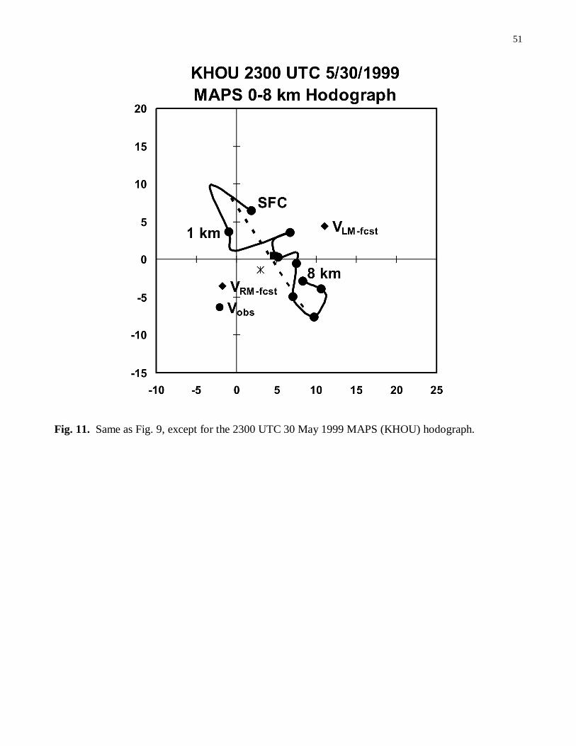
51

Fig. 11. Same as Fig. 9, except for the 2300 UTC 30 May 1999 MAPS (KHOU) hodograph.

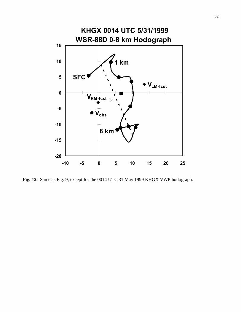
52

Fig. 12. Same as Fig. 9, except for the 0014 UTC 31 May 1999 KHGX VWP hodograph.

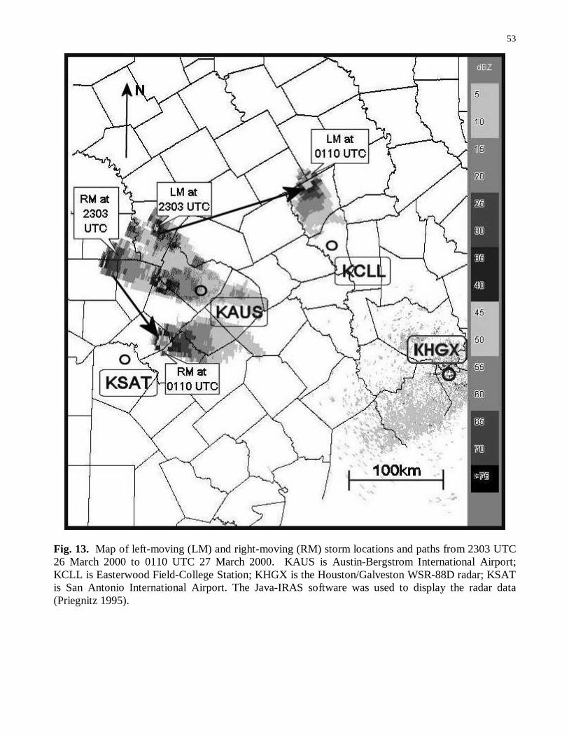
53

Fig. 13. Map of left-moving (LM) and right-moving (RM) storm locations and paths from 2303 UTC 26 March 2000 to 0110 UTC 27 March 2000. KAUS is Austin-Bergstrom International Airport; KCLL is Easterwood Field-College Station; KHGX is the Houston/Galveston WSR-88D radar; KSAT is San Antonio International Airport. The Java-IRAS software was used to display the radar data (Priegnitz 1995).

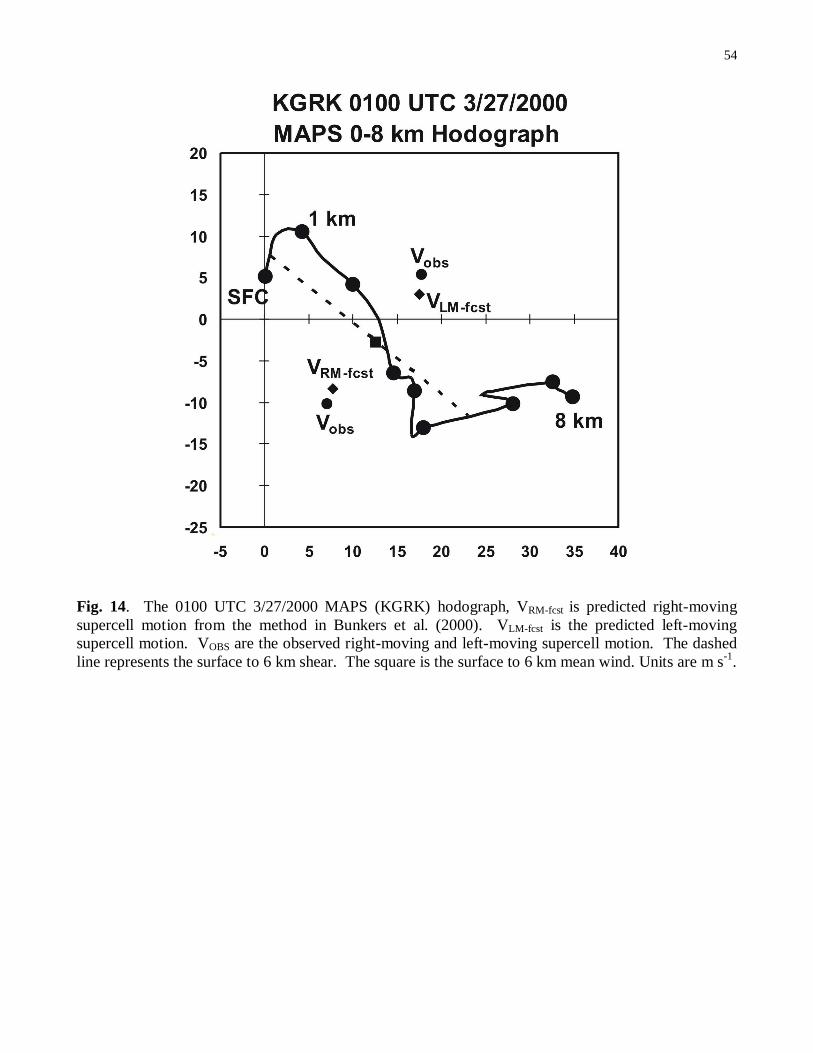
54

Fig. 14. The 0100 UTC 3/27/2000 MAPS (KGRK) hodograph, VRM-fcst is predicted right-moving supercell motion from the method in Bunkers et al. (2000). VLM-fcst is the predicted left-moving supercell motion. VOBS are the observed right-moving and left-moving supercell motion. The dashed line represents the surface to 6 km shear. The square is the surface to 6 km mean wind. Units are m s-1.

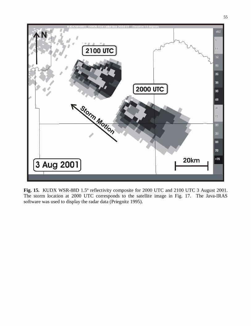
55

Fig. 15. KUDX WSR-88D 1.5º reflectivity composite for 2000 UTC and 2100 UTC 3 August 2001. The storm location at 2000 UTC corresponds to the satellite image in Fig. 17. The Java-IRAS software was used to display the radar data (Priegnitz 1995).

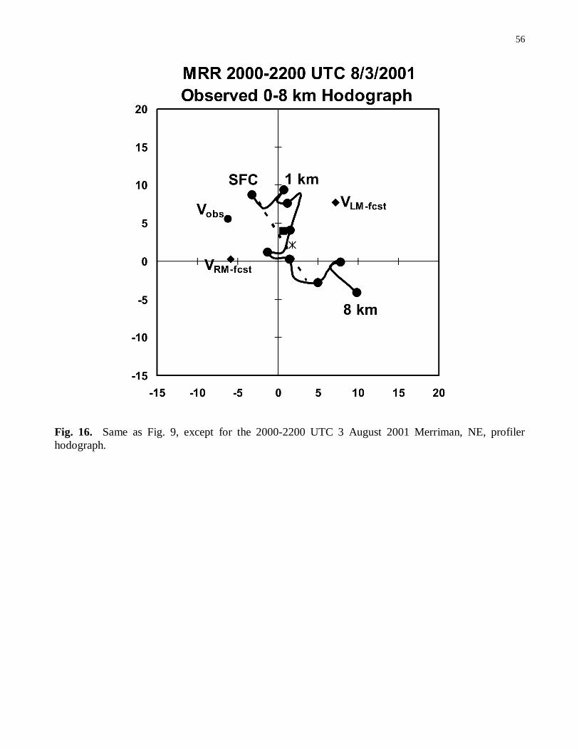
56

Fig. 16. Same as Fig. 9, except for the 2000-2200 UTC 3 August 2001 Merriman, NE, profiler hodograph.

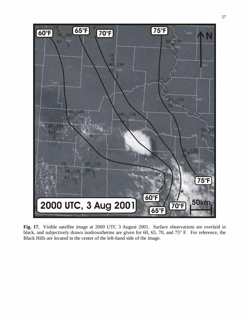
57

Fig. 17. Visible satellite image at 2000 UTC 3 August 2001. Surface observations are overlaid in black, and subjectively drawn isodrosotherms are given for 60, 65, 70, and 75° F. For reference, the Black Hills are located in the center of the left-hand side of the image.

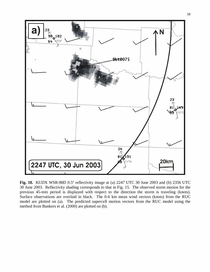
58

Fig. 18. KUDX WSR-88D 0.5º reflectivity image at (a) 2247 UTC 30 June 2003 and (b) 2356 UTC 30 June 2003. Reflectivity shading corresponds to that in Fig. 15. The observed storm motion for the previous 45-min period is displayed with respect to the direction the storm is traveling (knots). Surface observations are overlaid in black. The 0-6 km mean wind vectors (knots) from the RUC model are plotted on (a). The predicted supercell motion vectors from the RUC model using the method from Bunkers et al. (2000) are plotted on (b).

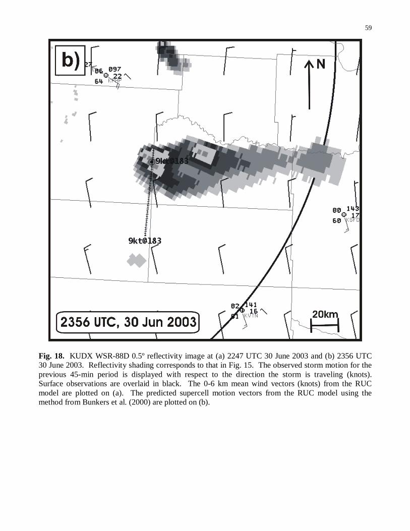
59

Fig. 18. KUDX WSR-88D 0.5º reflectivity image at (a) 2247 UTC 30 June 2003 and (b) 2356 UTC 30 June 2003. Reflectivity shading corresponds to that in Fig. 15. The observed storm motion for the previous 45-min period is displayed with respect to the direction the storm is traveling (knots). Surface observations are overlaid in black. The 0-6 km mean wind vectors (knots) from the RUC model are plotted on (a). The predicted supercell motion vectors from the RUC model using the method from Bunkers et al. (2000) are plotted on (b).

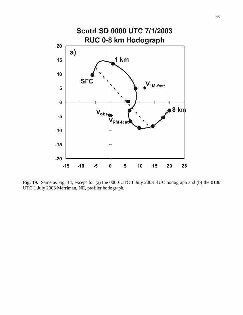
60

Fig. 19. Same as Fig. 14, except for (a) the 0000 UTC 1 July 2003 RUC hodograph and (b) the 0100 UTC 1 July 2003 Merriman, NE, profiler hodograph.

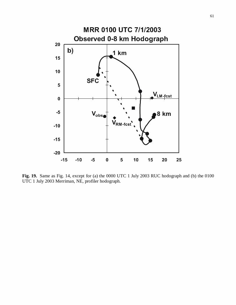
61

Fig. 19. Same as Fig. 14, except for (a) the 0000 UTC 1 July 2003 RUC hodograph and (b) the 0100 UTC 1 July 2003 Merriman, NE, profiler hodograph.