PHYSICAL REVIEW A 87, 013810 (2013)

Optical vortex solitary wave in a bounded nematic-liquid-crystal cell

Antonmaria A. Minzoni,1 Luke W. Sciberras,2 Noel F. Smyth,2 and Annette L. Worthy2

1Fenomenos Nonlineales y Mecanica (FENOMEC), Department of Mathematics and Mechanics, Instituto de Investigacion en MatematicasAplicadas y Sistemas, Universidad Nacional Autonoma de Mexico, 01000 Mexico Distrito Federal, Mexico

2School of Mathematics and Applied Statistics, University of Wollongong, Northfields Avenue, Wollongong, New South Wales, Australia 2522(Received 1 November 2012; published 14 January 2013)

Modulation theory, based on a Lagrangian formulation of the governing equations, is used to investigatethe propagation of a nonlinear, nonlocal optical vortex solitary wave in a finite nematic-liquid-crystal cell. Thenematic response to the vortex is calculated using the approach of the method of images (MOI). It is demonstratedthat the MOI is a reliable alternative to the usual Fourier series solution as it requires an order of magnitudefewer terms to obtain excellent agreement with numerical solutions. It is found that the cell walls, in additionto repelling the optical vortex solitary wave, as for an optical solitary wave, can destabilize it due to the fixeddirector orientation at the walls. A linearized stability analysis is used to explain and analyze this instability.In particular, the minimum distance of approach of a stable vortex to the wall is determined from the stabilityanalysis. Good agreement is found with numerical minimum approach distances.

DOI: 10.1103/PhysRevA.87.013810 PACS number(s): 42.65.Tg, 42.70.Df, 05.45.Yv

I. INTRODUCTION

Optical vortices have been studied for many years, begin-ning with the initial theoretical work of Nye and Berry [1], whomathematically studied phase dislocations in a wave train. Anoptical vortex is a light beam which has an azimuthal twist,resulting in a corkscrewlike structure, such that its azimuthalphase increases by 2nπ , with n an integer, over one twist, withthe integer n being referred to as the charge of the vortex.The term vortex comes from its similarity to a vortex in fluidflow. The amplitude of the optical field is zero at the center ofthe vortex to adjust to the phase singularity there. It has beenfound that optical vortices exist in numerous media, includingphotorefractive lattices [2,3], rubidium vapor cells [4,5], andBose-Einstein condensates [6]. A medium of intense interestdue to its potential application in all-optical devices [7–9] is anematic liquid crystal (NLC). The reason for this interest is thatin a NLC, nonlinear effects can be observed over millimeterdistances at milliwatt optical power levels due to the “huge”nonlinearity of a NLC [10]. In addition, the optical response ofa NLC is termed nonlocal in that the response of the nematicextends far beyond the waist of the optical beam perturbing thenematic. This nonlocal response is vital in that it stops the usualcatastrophic collapse of two-dimensional (2D) bulk solitarywaves [7,11,12]. In addition, optical vortex solitary waves areunstable in local media, but are stable in nonlocal media,such as nematic liquid crystals, as the symmetry-breakingmode-2 azimuthal instability is suppressed if the nonlocalityis large enough [13,14]. In contrast to local media [11,15],optical vortex solitary waves in nonlocal media have receivedconsiderably less attention, especially in a NLC [14,16–21].

In experiments, an optical vortex can be generated when adiffracting beam with a smooth wave front is input througha computer-generated holographic mask [4,22], creating ahelical phase ramp whose thickness increases around the center(the singularity) of the vortex by 2nπ , where n = 1,2, . . .

is the topological charge of the vortex [17]. A gradient ofcirculation is forced in the angular variable around the vortex,with the amplitude zero at the center to compensate for thephase singularity, as discussed above. Optical solitary waves,

termed nematicons, and optical vortex solitary waves form ina NLC due to a balance between the diffractive spreading ofan optical beam and the nonlinear self-focusing of the beamdue to the nonlinear dependence of the refractive index ofthe nematic on the beam intensity [7,12]. The refractive indexof the nematic changes due to the physical rotation of thethreadlike nematic molecules. There is an added complicationin that when the electric fields of the beam and the moleculardirector are orthogonal, a minimum beam power is requiredto rotate the molecules, known as the Freedericksz threshold[9,10,23,24]. To aid in overcoming this threshold so that opticalbeams of milliwatt powers can be used to form nematiconsand optical vortex solitary waves, the nematic molecules arepretilted at an angle θ0 ∼ π/4 to the optical wave front, as theFreedericksz threshold is zero when θ0 = π/4. There are twocommon methods to generate this pretilting, with the first beingto apply an external static electric field to the liquid-crystalcell. The second method is to “rub” the cell walls, creatinga static charge at the cell walls, which induces a rotation inthe nematic molecules at the cell walls. This rotation thenpropagates into the bulk of the nematic due to intermolecularelastic forces, i.e., the nonlocality of the liquid crystal [10]. Inthe present paper, the second pretilt method will be used. Theresponse of the nematic is dependent upon the chosen methodof pretilt. In the case of rubbing, there is a linear (1D) orlogarithmic (2D) decay of the nematic response away from thebeam’s center [25,26]. This implies that all of the moleculesof the nematic are affected by the presence of a beam in thecell [26], so that, in particular, boundary conditions at thecell walls must be properly accounted for Refs. [25,26]. Incontrast, when the first pretilt method, based on an externalstatic electric field, is used, there is an exponential decay ofthe nematic response away from the beam. As a consequence,the effect of the cell walls can be neglected [27–30] for beampropagation near the center of a cell, as the cell-to-beam widthratio is around 20 to 30 [31,32]. In the nematicon case, it hasbeen observed both experimentally [33] and theoretically in1D [25,26] and 2D [34] that cell walls act repulsively towards anematicon.

013810-11050-2947/2013/87(1)/013810(11) ©2013 American Physical Society

MINZONI, SCIBERRAS, SMYTH, AND WORTHY PHYSICAL REVIEW A 87, 013810 (2013)

In the present work, the behavior and propagation ofan optical vortex solitary wave in a finite nematic cell isinvestigated. As the present work is concerned with vortexsolitary waves, which are nonlinear, and not with linear opticalvortices, from now on the term optical vortex will mean avortex solitary wave. Particular attention is paid to the effectthat the cell boundaries have on both the propagation and thestability of an optical vortex. To achieve this task, a blend ofan exact solution found using the method of images (MOI)and a trial function, coupled with a Lagrangian formulationand modulation theory [35], is used. Modulation theory basedon suitable trial functions has been found to be a useful andsuccessful technique for giving results in excellent agreementwith full numerical solutions [14,16,18,27,28,30,36] andexperimental results [37,38]. In addition, it is found that themethod of images possesses distinct advantages over othersolution methods in that it requires an order of magnitudefewer terms to obtain accurate solutions [34]. This paper thenreconfirms the usefulness of the MOI [34] in another contextas a viable alternative to the standard Fourier series solutionto provide evolutionary information. In addition, the MOI isused to analyze the linearized stability of an optical vortexdue to its interaction with the cell walls. It is found that thisinteraction destabilizes the vortex if it approaches too closelyto a wall. This is because the director angle is fixed at thewall due to anchoring. Previous studies have shown that anoptical vortex is stable in a nematic liquid crystal due tononlocality causing a nonzero director angle under the coreof the vortex [14]. This effect cannot happen near the walls ofa cell due to anchoring. A similar instability has been foundwhen an optical vortex refracts at a nonlinear refractive indexinterface in a nematic liquid crystal [16], where this interfaceis caused by the director having two different orientations oneither side of the interface [39–41]. These two instabilitiesare not exactly the same as the director has more freedomto rotate at the refractive index interface. The linearizedstability analysis illuminates the instability mechanism andis used to determine the minimum distance of approach to acell wall before instability occurs. These stability results arethen compared with full numerical solutions of the governingequations.

II. GOVERNING EQUATIONS

An optical vortex is input at the NLC-air interface of a cellfilled with a nematic liquid crystal. The z direction is definedto be the propagation direction down the cell, with the (x,y)plane orthogonal to this. The optical beam is polarized so thatits electric field is in the x direction. The nematic moleculeshave been arranged in a planar configuration in the (x,z) plane.The cell walls have also undergone a pretreatment known as“rubbing,” whereby a static charge is created at the cell walls,causing the molecules closest to the boundaries to rotate inthe (x,z) plane. Intermolecular elastic forces then propagatethis director rotation into the bulk of the liquid crystal. Thispretreatment results in the molecular director being prerotatedin the (x,z) plane at an angle θ0 to the z direction, which helps toovercome the Freedericksz threshold [12,24], so that milliwattpower optical beams can self-focus and form nematicons oroptical vortices (vortex solitary waves) with nonlinear self-

focusing balancing diffractive spreading [7]. The Freederickszthreshold can be reduced to exactly zero if the pretilt angleθ0 = π/4 [42]. The optical field causes an extra rotation θ

of the director, so that the total director angle is θ0 + θ tothe z direction. For milliwatt optical beam powers, this extrarotation is small and |θ | � |θ0|. In this small extra rotationlimit, the nondimensional equations governing the propagationof the optical vortex beam in the paraxial approximation are[25,26,33,34]

i∂E

∂z+ 1

2∇2E + 2θE = 0, (1)

ν∇2θ + 2|E|2 = 0. (2)

The Laplacian ∇2 is in the (x,y) plane [7,12,27]. E is thecomplex valued envelope of the electric field of the opticalbeam. The nonlocality parameter ν is related to the elasticresponse of the nematic and experimentally is of the orderof O(100) [37]. As the nematic is uniform, the walk-offangle, which is the angle between the Poynting vector andthe extraordinary beam’s wave vector, is also constant andso can be removed from the governing equations by a phasefactor [28,43], which has been done in deriving (1). The cellgeometry is rectangular in the cross section, with 0 � x � Lx

and 0 � y � Ly . Anchoring boundary conditions give that thetotal director angle is fixed at the cell walls, so that θ = 0 at theboundaries x = 0,Lx and y = 0,Ly . The nematic equations (1)and (2) are general and describe nonlinear wave propagation inmany media with a diffusive response, such as photorefractivecrystals [44,45] and thermal media [46–48].

The governing equations (1) and (2) have the Lagrangian

L = i(E∗Ez − EE∗z ) − |∇E|2 + 2θ |E|2. (3)

The asterisk superscript denotes the complex conjugate. Thelinear director equation (2) can be solved exactly in terms of aGreen’s function G(x,y,x ′,y ′), with

θ = 2

ν

∫ Ly

0

∫ Lx

0|E(x ′,y ′,z)|2G(x,y,x ′,y ′)dx ′dy ′. (4)

III. EVOLUTION EQUATIONS

In general, the governing equations (1) and (2) for theevolution of a nonlinear optical beam in a nematic liquidcrystal have no known exact solitary wave or vortex solutions[27]. To gain additional insights into the underlying physicsand mechanics of these nonlinear beams that full numericalsolutions cannot supply, averaged Lagrangian techniques [35]have proved useful, as discussed in Sec. I. The analysispresented here combines an exact solution and a trial-function-based averaged Lagrangian method [18,26,34]. A Gaussianprofile is used for the trial function of the electric field of theoptical vortex and is

E = (are−r2/w2 + ig)eiψ+inφ, (5)

where

ψ = σ + Vx (x − ξ ) + Vy (y − η) , (6)

013810-2

OPTICAL VORTEX SOLITARY WAVE IN A BOUNDED . . . PHYSICAL REVIEW A 87, 013810 (2013)

30 40 50 60 70

x

30

40

50

60

70

y

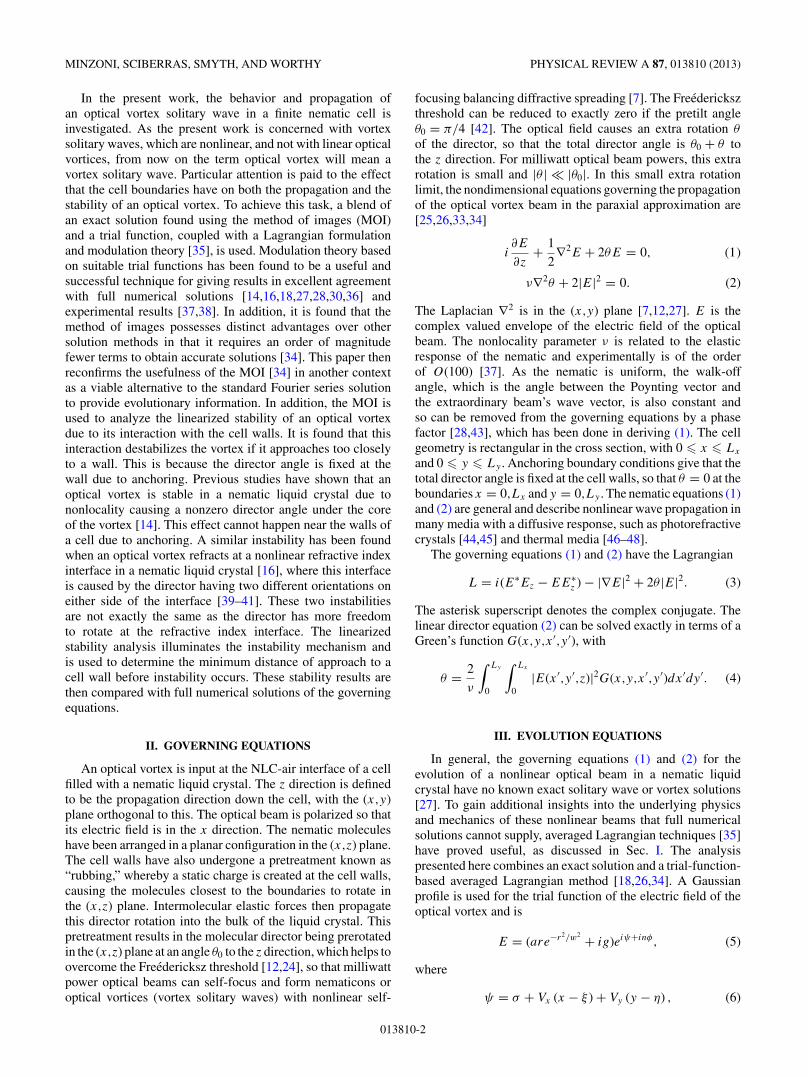
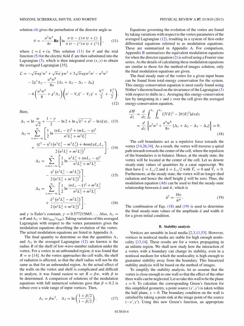
FIG. 1. (Color online) Initial profile of an optical vortex for thetrial function (5) with g = 0 and n = 1.

and r and φ are polar coordinates based on the center of thevortex,

r2 = (x − ξ )2 + (y − η)2 , φ = tan−1

(y − η

x − ξ

). (7)

This trial function for the optical vortex is illustrated in Fig. 1.The first term in the trial function for the electric field is anoptical vortex of amplitude A = awe−1/2/

√2, with this peak

occurring at radius r = w/√

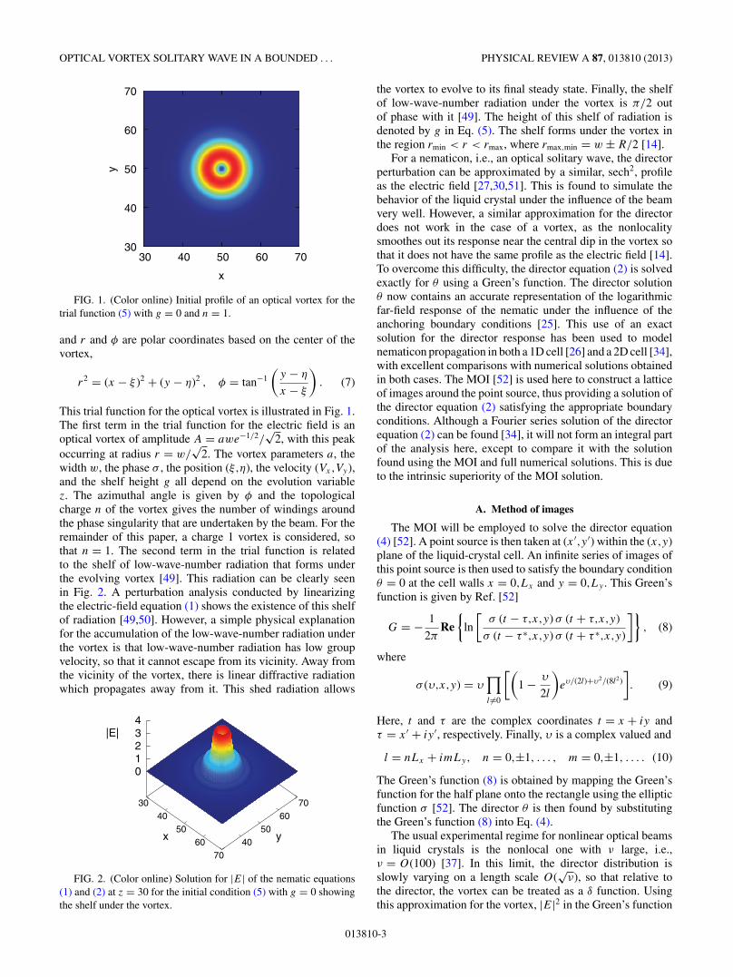
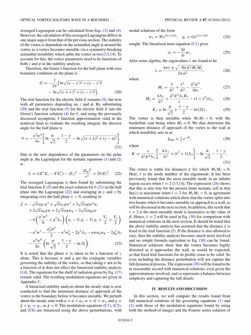
2. The vortex parameters a, thewidth w, the phase σ , the position (ξ,η), the velocity (Vx,Vy),and the shelf height g all depend on the evolution variablez. The azimuthal angle is given by φ and the topologicalcharge n of the vortex gives the number of windings aroundthe phase singularity that are undertaken by the beam. For theremainder of this paper, a charge 1 vortex is considered, sothat n = 1. The second term in the trial function is relatedto the shelf of low-wave-number radiation that forms underthe evolving vortex [49]. This radiation can be clearly seenin Fig. 2. A perturbation analysis conducted by linearizingthe electric-field equation (1) shows the existence of this shelfof radiation [49,50]. However, a simple physical explanationfor the accumulation of the low-wave-number radiation underthe vortex is that low-wave-number radiation has low groupvelocity, so that it cannot escape from its vicinity. Away fromthe vicinity of the vortex, there is linear diffractive radiationwhich propagates away from it. This shed radiation allows

30 40

50 60

70 40

50 60

70

0 1 2 3 4

x y

|E|

FIG. 2. (Color online) Solution for |E| of the nematic equations(1) and (2) at z = 30 for the initial condition (5) with g = 0 showingthe shelf under the vortex.

the vortex to evolve to its final steady state. Finally, the shelfof low-wave-number radiation under the vortex is π/2 outof phase with it [49]. The height of this shelf of radiation isdenoted by g in Eq. (5). The shelf forms under the vortex inthe region rmin < r < rmax, where rmax,min = w ± R/2 [14].

For a nematicon, i.e., an optical solitary wave, the directorperturbation can be approximated by a similar, sech2, profileas the electric field [27,30,51]. This is found to simulate thebehavior of the liquid crystal under the influence of the beamvery well. However, a similar approximation for the directordoes not work in the case of a vortex, as the nonlocalitysmoothes out its response near the central dip in the vortex sothat it does not have the same profile as the electric field [14].To overcome this difficulty, the director equation (2) is solvedexactly for θ using a Green’s function. The director solutionθ now contains an accurate representation of the logarithmicfar-field response of the nematic under the influence of theanchoring boundary conditions [25]. This use of an exactsolution for the director response has been used to modelnematicon propagation in both a 1D cell [26] and a 2D cell [34],with excellent comparisons with numerical solutions obtainedin both cases. The MOI [52] is used here to construct a latticeof images around the point source, thus providing a solution ofthe director equation (2) satisfying the appropriate boundaryconditions. Although a Fourier series solution of the directorequation (2) can be found [34], it will not form an integral partof the analysis here, except to compare it with the solutionfound using the MOI and full numerical solutions. This is dueto the intrinsic superiority of the MOI solution.

A. Method of images

The MOI will be employed to solve the director equation(4) [52]. A point source is then taken at (x ′,y ′) within the (x,y)plane of the liquid-crystal cell. An infinite series of images ofthis point source is then used to satisfy the boundary conditionθ = 0 at the cell walls x = 0,Lx and y = 0,Ly . This Green’sfunction is given by Ref. [52]

G = − 1

2πRe

{ln

[σ (t − τ,x,y) σ (t + τ,x,y)

σ (t − τ ∗,x,y) σ (t + τ ∗,x,y)

]}, (8)

where

σ (υ,x,y) = υ∏l �=0

[(1 − υ

2l

)eυ/(2l)+υ2/(8l2)

]. (9)

Here, t and τ are the complex coordinates t = x + iy andτ = x ′ + iy ′, respectively. Finally, υ is a complex valued and

l = nLx + imLy, n = 0,±1, . . . , m = 0,±1, . . . . (10)

The Green’s function (8) is obtained by mapping the Green’sfunction for the half plane onto the rectangle using the ellipticfunction σ [52]. The director θ is then found by substitutingthe Green’s function (8) into Eq. (4).

The usual experimental regime for nonlinear optical beamsin liquid crystals is the nonlocal one with ν large, i.e.,ν = O(100) [37]. In this limit, the director distribution isslowly varying on a length scale O(

√ν), so that relative to

the director, the vortex can be treated as a δ function. Usingthis approximation for the vortex, |E|2 in the Green’s function

013810-3

MINZONI, SCIBERRAS, SMYTH, AND WORTHY PHYSICAL REVIEW A 87, 013810 (2013)

solution (4) gives the perturbation of the director angle as

θ = −a2w4

4νRe

{ln

σ (t − ζ ) σ (t + ζ )

σ (t − ζ ∗) σ (t + ζ ∗)

}, (11)

where ζ = ξ + iη. This solution (11) for θ and the trialfunction (5) for the electric field E are then substituted into theLagrangian (3), which is then integrated over (x,y) to obtainthe averaged Lagrangian [35],

L = −√πag′w3 + √

πa′gw3 + 3√

πagw2w′ − a2w2

− 2g2�2 − a4w8

8ν[�1 + �2 − �3 − �4]

− 4

(a2w4

8+ g2�1

)(σ ′ − Vxξ

′ − Vyη′ + V 2

x

2+ V 2

y

2

).

(12)

Here,

�1 = lnw√

2+ 1 − γ

2− ln 2 + ln

√ξ 2 + η2 − ln (ξη) , (13)

�2 =∞∑

n,m=−∞

[1

2ln

(nLx − ξ )2 + (mLy − η)2

n2L2x + m2L2

y

+ (ξ 2 − η2)(n2L2

x − m2L2y

) + 4nmξηLxLy

2(n2L2

x + m2L2y

)2

], (14)

�3 =∞∑

n,m=−∞

[1

2ln

n2L2x + (mLy − η)2

n2L2x + m2L2

y

− η2(n2L2

x − m2L2y

)2(n2L2

x + m2L2y

)2

], (15)

�4 =∞∑

n,m=−∞

[1

2ln

(nLx − ξ )2 + m2L2y

n2L2x + m2L2

y

+ ξ 2(n2L2

x − m2L2y

)2(n2L2

x + m2L2y

)2

], (16)

and γ is Euler’s constant, γ = 0.577215665 . . .. Also, �1 =wR and �2 = ln(rmax/rmin). Taking variations of this averagedLagrangian with respect to the vortex parameters gives themodulation equations describing the evolution of the vortex.The actual modulation equations are listed in Appendix A.

The final quantity to determine so that the quantities �1

and �2 in the averaged Lagrangian (12) are known is theradius R of the shelf of low-wave-number radiation under thevortex. For a vortex in an unbounded region, it was found thatR = w [14]. As the vortex approaches the cell walls, the shelfof radiation is affected, so that the shelf radius will not be thesame as that for an unbounded region. As the actual effect ofthe walls on the vortex and shelf is complicated and difficultto analyze, it was found easiest to set R = βw, with β tobe determined. A comparison of solutions of the modulationequations with full numerical solutions gave that β = 0.2 isrobust over a wide range of input vortices. Then,

�1 = βw2, �2 = ln

(1 + β/2

1 − β/2

). (17)

Equations governing the evolution of the vortex are foundby taking variations with respect to the vortex parameters of theaveraged Lagrangian (12), resulting in a system of first-orderdifferential equations referred to as modulation equations.These are summarized in Appendix A. For comparison,Appendix B summarizes the equivalent modulation equationsfor when the director equation (2) is solved using a Fourier sineseries. As the details of calculating these modulation equationsare similar to those for the method-of-images solution, onlythe final modulation equations are given.

The final steady state of the vortex for a given input beamcan be found from total-energy conservation for the system.This energy-conservation equation is most easily found usingNother’s theorem based on the invariance of the Lagrangian (3)with respect to shifts in z. Averaging this energy-conservationlaw by integrating in x and y over the cell gives the averagedenergy-conservation equation,

dH

dz= d

dz

∫ Ly

0

∫ Lx

0[|∇E|2 − 2θ |E|2]dxdy

= d

dz

{a2w2 + a4w8

8ν[�1 + �2 − �3 − �4]

}= 0.

(18)

The cell boundaries act as a repulsive force towards thevortex [14,26,34]. As a result, the vortex will traverse a spiralpath inwards towards the center of the cell, where the repulsionof the boundaries is in balance. Hence, at the steady state, thevortex will be located at the center of the cell. Let us denotesteady-state values of quantities by a carat superscript. Wethen have ξ = Lx/2 and η = Ly/2 with Vx = 0 and Vy = 0.Furthermore, at the steady state, the vortex will no longer shedradiation and hence the shelf height g will be zero. Thus, themodulation equation (A6) can be used to find the steady-staterelationship between a and w, which is

a2 = 16ν

w6. (19)

The combination of Eqs. (18) and (19) is used to determinethe final steady-state values of the amplitude a and width w

for a given initial condition.

B. Stability analysis

Vortices are unstable in local media [2,3,11,53]. However,vortices in nonlocal media are stable for high enough nonlo-cality [13,14]. These results are for a vortex propagating inan infinite region. We shall now study how the interaction ofa vortex with a boundary can change its stability, even in anonlocal medium for which the nonlocality is high enough toguarantee stability away from the boundary. This linearizedstability analysis will be based on the method of images.

To simplify the stability analysis, let us assume that thevortex is close enough to one wall so that the effect of the otherthree walls can be neglected. Let us take this wall to be the planex = 0. To calculate the corresponding Green’s function forthis simplified geometry, a point source (x ′,y ′) is taken withinthe half plane, x > 0. The boundary condition on the wall issatisfied by taking a point sink at the image point of the source(−x ′,y ′). Using this new Green’s function, an appropriate

013810-4

OPTICAL VORTEX SOLITARY WAVE IN A BOUNDED . . . PHYSICAL REVIEW A 87, 013810 (2013)

averaged Lagrangian can be calculated from Eqs. (3) and (4).However, the calculation of this averaged Lagrangian differs inone major aspect from that of the previous section. The stabilityof the vortex is dependent on the azimuthal angle φ around thevortex as a vortex becomes unstable via a symmetry-breakingazimuthal instability which splits the vortex in two [13,14]. Toaccount for this, the vortex parameters need to be functions ofboth z and φ in the stability analysis.

Therefore, the Green’s function for the half plane with zeroboundary condition on the plane is

G = − 1

2π

[ln

√(x − x ′)2 + (y − y ′)2

− ln√

(x + x ′)2 + (y − y ′)2]. (20)

The trial function for the electric field E remains (5), but nowwith all parameters depending on z and φ. By substituting(20) and the trial function (5) for the electric field E into theGreen’s function solution (4) for θ , and using the previouslydiscussed asymptotic δ function approximation valid in thenonlocal limit to evaluate the resulting integral, the directorangle for the half plane is

θ = −a2w4

4ν

[ln

w√2

+ 1 − γ

2− ln

√(x + ξ )2 + (y − η)2

].

(21)

Due to the new dependence of the parameters on the polarangle φ, the Lagrangian for the nematic equations (1) and (2)is

L = i(E∗Ez − EE∗z ) − |Er |2 − |Eφ|2

r2+ 2θ |E|2. (22)

The averaged Lagrangian is then found by substituting thetrial function E (5) and the exact solution for θ (21) in the halfplane into the Lagrangian (22) and averaging in x and y byintegrating over the half plane x > 0, resulting in

L = −√πagzw

3 + √πazgw3 + 3

√πagw2wz

+ 2√

πaφgw + 2√

πagwφ − 2√

πagφw

− 4

(a2w4

8+ g2�1

) (σz − Vxξz − Vyηz + Vx

2+ Vy

2

)

− a2w2 − a2φw2

2− a2w2

φ − 2g2�2 − awaφwφ − 2g2φ�2

− a4w8

8ν

(ln

w√2

+ 1 − γ

2− ln 2ξ

). (23)

It is noted that the phase σ is taken to be a function of z

alone. This is because w and g are the conjugate variablesgoverning the stability of the vortex, so that taking σ not to bea function of φ does not affect the linearized stability analysis[14]. The equations for the shelf of radiation given by Eq. (17)remain valid. The resulting modulation equations are given inAppendix C.

A linearized stability analysis about the steady state is nowconducted to find the minimum distance of approach of thevortex to the boundary before it becomes unstable. We perturbabout the steady state with a = a + a1, w = w + w1, and g =g + g1 = g1, as g = 0. The modulation equations (C1), (C2),and (C6) are linearized using the above perturbations, with

modal solutions of the form

w1 = Wei(λz+�φ), g1 = Gei(λz+�φ) (24)

sought. The linearized mass equation (C1) gives

a1 = −2a

ww1. (25)

After some algebra, the eigenvalues λ are found to be

λ = 4π� ±√

−8πw2M1M2

2πw2, (26)

where

M1 = 3

w2+ �2

w2− a2w4

16ν, (27)

M2 = 4�1

w2+ a2w4�1K1

ν− (1 + �2)�2, (28)

K1 = lnw√

2+ 1 − γ

2− ln (2ξ ) . (29)

The vortex is then unstable when M1M2 > 0, with theborderline case being when M2 = 0. We thus determine theminimum distance of approach of the vortex to the wall atwhich instability sets in as

ξmin = 12 e−K, (30)

where

K = ν

a2w4�1

[−4�1

w2+ (�2 + 1)�2

]− ln

w√2

− 1 − γ

2.

(31)

The vortex is stable for distances ξ for which M1M2 < 0.Here, � is the mode number of the eigenmode. It has beenpreviously found that the most unstable mode in an infiniteregion occurs when � = 2 [13,14]. The expression (26) showsthat this is also true for the present finite nematic cell in thatIm(λ) is maximum when � = 2 for M1M2 > 0, in agreementwith numerical solutions which show that the vortex splits intotwo beams when it becomes unstable on approach to a wall, aswill be discussed in the next section. In addition, this result that� = 2 is the most unstable mode is insensitive to the value ofβ. Hence, � = 2 will be used in Eq. (30) for comparison withnumerical solutions in the next section. It should be noted thatthe above stability analysis has assumed that the distance ξ isfixed in the trial function (5). If the distance is also allowed tovary, then the stability analysis becomes much more involvedand no simple formula equivalent to Eq. (30) can be found.Numerical solutions show that the vortex becomes highlydistorted as it approaches the wall, as would be expected,so that fixed trial functions for its profile cease to be valid. Soeven including the distance perturbation will not capture thefull dynamical process. The expression (30) will be found to bein reasonable accord with numerical solutions, even given theapproximations involved, and so represents a balance betweensimplicity and capturing the full details.

IV. RESULTS AND DISCUSSION

In this section, we will compare the results found fromfull numerical solutions of the governing equations (1) and(2) with those of the modulation equations found by usingboth the method-of-images and the Fourier series solution of

013810-5

MINZONI, SCIBERRAS, SMYTH, AND WORTHY PHYSICAL REVIEW A 87, 013810 (2013)

the director equation (2). The modulation equations, givenin Appendices A and B, were solved using the standardfourth-order Runge-Kutta method. The full numerical solutionof the electric-field equation (1) was found using second-ordercentered differences for the Laplacian ∇2E and a second-order predictor-corrector method, based on the second-orderRunge-Kutta method, to advance forward in z, which is thepropagation direction. The director equation (2) was solvedusing centered second-order differences for the Laplacian∇2θ and Jacobi iteration to solve the resulting linear system.The initial condition for the optical beam envelope for thenumerical solutions is the trial function (5) with the shelfheight g equal to zero, as the vortex has not started to shedradiation. To satisfy the stability criteria and maintain accuracy,the step sizes used were �x = �y = 0.2 and �z = 0.001.The propagation length used was z = 500, which is a typicalnondimensional cell length [37]. The numerical investigationfor the propagation of an optical vortex was conducted withina square NLC cell with nondimensional width and breadth(Lx,Ly) = (100,100).

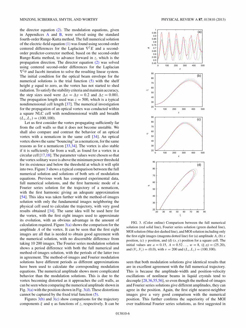
Let us first consider the vortex propagating sufficiently farfrom the cell walls so that it does not become unstable. Weshall also compare and contrast the behavior of an opticalvortex with a nematicon in the same cell [34]. An opticalvortex shows the same “bouncing” as a nematicon, for the samereasons as for a nematicon [33,34]. The vortex is also stableif it is sufficiently far from a wall, as found for a vortex in acircular cell [17,18]. The parameter values were chosen so thatthe vortex solitary wave is above the minimum power thresholdfor its existence and below the threshold at which it will splitinto two. Figure 3 shows a typical comparison between the fullnumerical solution and solutions of both sets of modulationequations. Previous work has compared experimental data,full numerical solutions, and the first harmonic mode of aFourier series solution for the trajectory of a nematicon,with the first harmonic giving an adequate approximation[54]. This idea was taken further with the method-of-imagessolution with only the fundamental images neighboring thephysical cell used to calculate the trajectory, with very goodresults obtained [34]. The same idea will be used here forthe vortex, with the first eight images used to approximateits evolution, with an obvious advantage in the amount ofcalculation required. Figure 3(a) shows the comparison for theamplitude A of the vortex. It can be seen that the first eightimages are all that is needed to obtain good agreement withthe numerical solution, with no discernible difference fromtaking 10 200 images. The Fourier series modulation solutionshows a period difference with both the full numerical andmethod-of-images solution, with the periods of the latter twoin agreement. The method-of-images and Fourier modulationsolutions have different periods as different approximationshave been used to calculate the corresponding modulationequations. The numerical amplitude shows more complicatedbehavior than the modulation solutions. This is due to thevortex becoming distorted as it approaches the cell walls, ascan be seen when comparing the numerical amplitude shown inFig. 3(a) with the position shown in Fig. 3(d). These distortionscannot be captured by the fixed trial function (5).

Figures 3(b) and 3(c) show comparisons for the trajectorycomponents ξ and η as functions of z, respectively. It can be

0.45 0.5

0.55 0.6

0.65 0.7

0.75 0.8

0.85 0.9

0.95 1

0 100 200 300 400 500

z

(a)

20

30

40

50

60

70

80

90

0 100 200 300 400 500

ξ

z

(b)

20

30

40

50

60

70

80

90

0 100 200 300 400 500

η

z

(c)

20

30

40

50

60

70

80

90

20 30 40 50 60 70 80 90

η

ξ

(d)

A

FIG. 3. (Color online) Comparison between the full numericalsolution (red solid line), Fourier series solution (green dashed line),MOI solution (blue dot-dashed line), and MOI solution including onlythe first eight images (magenta dotted line) for (a) amplitude A, (b) x

position, (c) y position, and (d) (x,y) position for a square cell. Theinitial values are a = 0.15, A = 0.52 . . ., w = 8, (ξ,η) = (25,20),and (Vx,Vy) = (0,0), with ν = 200 and (Lx,Ly) = (100,100).

seen that both modulation solutions give identical results thatare in excellent agreement with the full numerical trajectory.This is because the amplitude-width and position-velocityoscillations of nonlinear beams in liquid crystals tend todecouple [28,36,55,56], so even though the method-of-imagesand Fourier series solutions give different amplitudes, they canagree in the position. Again, the first eight nearest-neighborimages give a very good comparison with the numericalposition. This further confirms the superiority of the MOIover traditional Fourier series solutions, as first suggested in

013810-6

OPTICAL VORTEX SOLITARY WAVE IN A BOUNDED . . . PHYSICAL REVIEW A 87, 013810 (2013)

3

4

5

6

7

7 8 9 10 11

Dis

tanc

e of

app

roac

h, ξ

Width, w

FIG. 4. (Color online) A comparison between the analytical sta-bility boundary (30) (red plus sign, +) with the full numerical solution(green crosses, ×) for (Vx,Vy) = (0.8,0) and the full numericalsolution (blue stars, *) for (Vx,Vy) = (1.5,0). The numerical stabilityboundary is the distance from the boundary at which instabilityfirst occurs. The initial conditions used were a given by Eq. (32),(ξ,η) = (50,100) for (Lx,Ly) = (100,200).

Ref. [34]. Taking the z direction to be into the page, the finalplot [Fig. 3(d)] shows the helical trajectory of the vortex as itpropagates down the liquid-crystal cell. The repulsive nature ofthe cell walls can be clearly seen. As the vortex was not givenan initial velocity, the vortex’s initial motion arises from thisrepulsive force. Thus, if the interaction with the boundary doesnot disturb the phase singularity at the center of the vortex, thecell walls will completely repel the vortex and stability will bemaintained, as in a circular cell [17,18]. Figure 3(d) confirmsthe conclusions drawn from Figs. 3(b) and 3(c), i.e., bothmodulation solutions are in agreement and are in excellentagreement with the numerical solution, and the first eightnearest-neighbor images give an excellent approximation tothe vortex trajectory.

A comparison between the analytical minimum distanceof approach for stability (30) and this minimum distanceas given by numerical solutions is shown in Fig. 4. Thisstability boundary is shown as a function of the initial widthw of the vortex for two different initial velocities, (Vx,Vy) =(0.8,0) and (Vx,Vy) = (1.5,0). The stability boundary (30) wasobtained using a small perturbation from the steady vortex.Hence, to obtain a comparison with numerical solutions, thenumerical initial condition must also be near a steady vortex.Equation (C6) of Appendix C gives the amplitude-widthrelation for the steady vortex as

a2w6 = 16ν. (32)

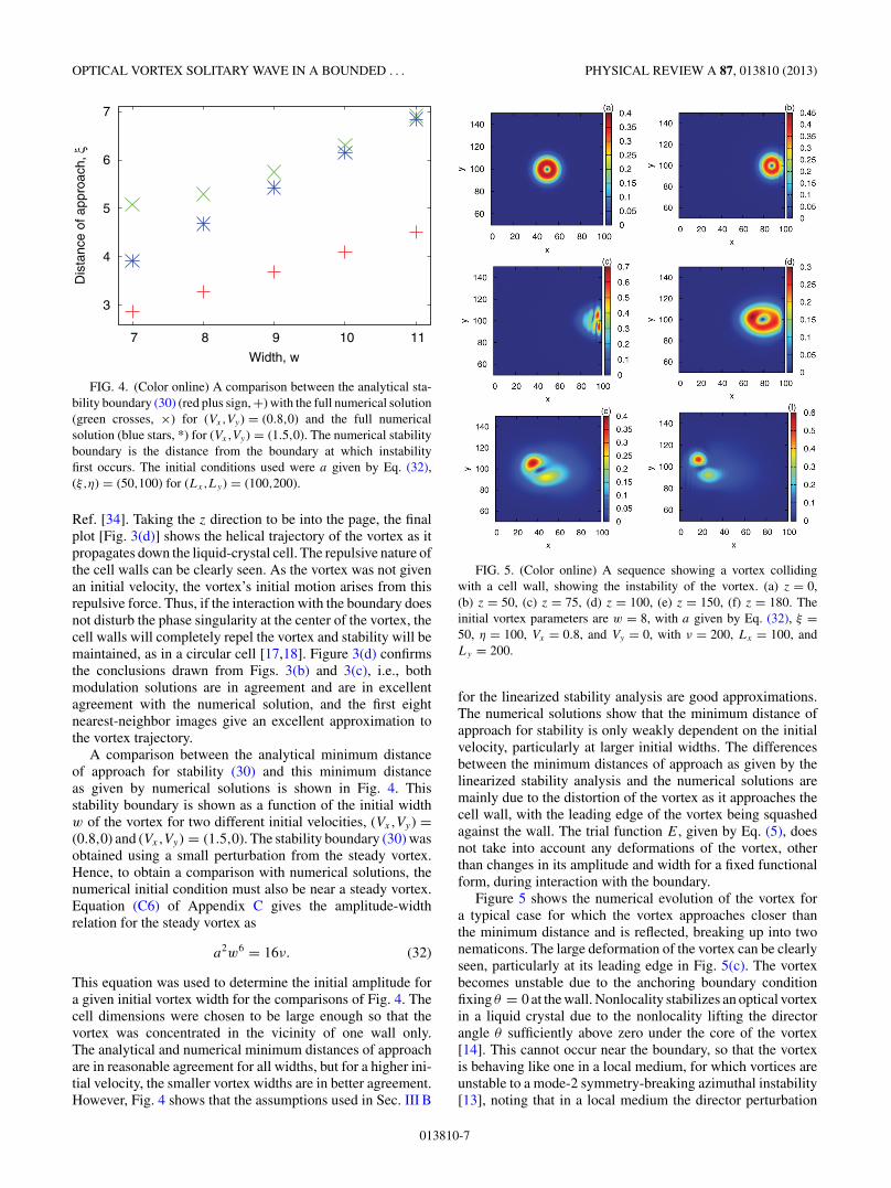
This equation was used to determine the initial amplitude fora given initial vortex width for the comparisons of Fig. 4. Thecell dimensions were chosen to be large enough so that thevortex was concentrated in the vicinity of one wall only.The analytical and numerical minimum distances of approachare in reasonable agreement for all widths, but for a higher ini-tial velocity, the smaller vortex widths are in better agreement.However, Fig. 4 shows that the assumptions used in Sec. III B

FIG. 5. (Color online) A sequence showing a vortex collidingwith a cell wall, showing the instability of the vortex. (a) z = 0,(b) z = 50, (c) z = 75, (d) z = 100, (e) z = 150, (f) z = 180. Theinitial vortex parameters are w = 8, with a given by Eq. (32), ξ =50, η = 100, Vx = 0.8, and Vy = 0, with ν = 200, Lx = 100, andLy = 200.

for the linearized stability analysis are good approximations.The numerical solutions show that the minimum distance ofapproach for stability is only weakly dependent on the initialvelocity, particularly at larger initial widths. The differencesbetween the minimum distances of approach as given by thelinearized stability analysis and the numerical solutions aremainly due to the distortion of the vortex as it approaches thecell wall, with the leading edge of the vortex being squashedagainst the wall. The trial function E, given by Eq. (5), doesnot take into account any deformations of the vortex, otherthan changes in its amplitude and width for a fixed functionalform, during interaction with the boundary.

Figure 5 shows the numerical evolution of the vortex fora typical case for which the vortex approaches closer thanthe minimum distance and is reflected, breaking up into twonematicons. The large deformation of the vortex can be clearlyseen, particularly at its leading edge in Fig. 5(c). The vortexbecomes unstable due to the anchoring boundary conditionfixing θ = 0 at the wall. Nonlocality stabilizes an optical vortexin a liquid crystal due to the nonlocality lifting the directorangle θ sufficiently above zero under the core of the vortex[14]. This cannot occur near the boundary, so that the vortexis behaving like one in a local medium, for which vortices areunstable to a mode-2 symmetry-breaking azimuthal instability[13], noting that in a local medium the director perturbation

013810-7

MINZONI, SCIBERRAS, SMYTH, AND WORTHY PHYSICAL REVIEW A 87, 013810 (2013)

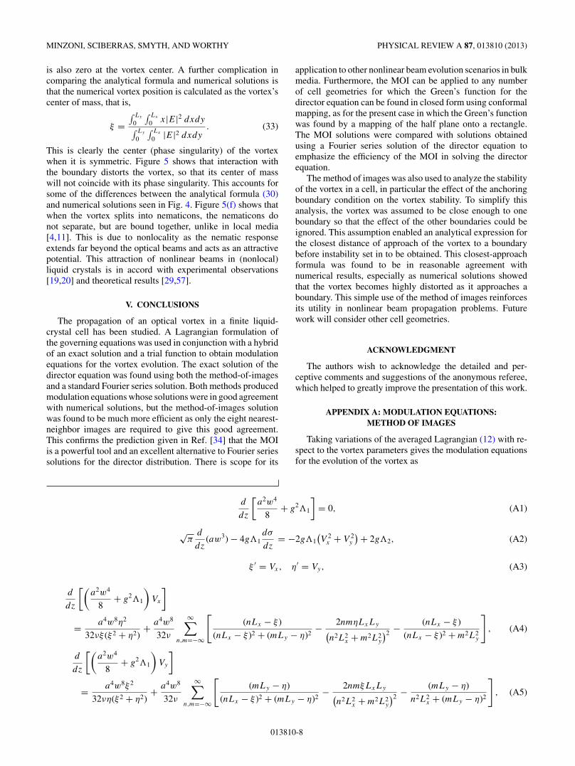
is also zero at the vortex center. A further complication incomparing the analytical formula and numerical solutions isthat the numerical vortex position is calculated as the vortex’scenter of mass, that is,

ξ =∫ Ly

0

∫ Lx

0 x|E|2 dxdy∫ Ly

0

∫ Lx

0 |E|2 dxdy. (33)

This is clearly the center (phase singularity) of the vortexwhen it is symmetric. Figure 5 shows that interaction withthe boundary distorts the vortex, so that its center of masswill not coincide with its phase singularity. This accounts forsome of the differences between the analytical formula (30)and numerical solutions seen in Fig. 4. Figure 5(f) shows thatwhen the vortex splits into nematicons, the nematicons donot separate, but are bound together, unlike in local media[4,11]. This is due to nonlocality as the nematic responseextends far beyond the optical beams and acts as an attractivepotential. This attraction of nonlinear beams in (nonlocal)liquid crystals is in accord with experimental observations[19,20] and theoretical results [29,57].

V. CONCLUSIONS

The propagation of an optical vortex in a finite liquid-crystal cell has been studied. A Lagrangian formulation ofthe governing equations was used in conjunction with a hybridof an exact solution and a trial function to obtain modulationequations for the vortex evolution. The exact solution of thedirector equation was found using both the method-of-imagesand a standard Fourier series solution. Both methods producedmodulation equations whose solutions were in good agreementwith numerical solutions, but the method-of-images solutionwas found to be much more efficient as only the eight nearest-neighbor images are required to give this good agreement.This confirms the prediction given in Ref. [34] that the MOIis a powerful tool and an excellent alternative to Fourier seriessolutions for the director distribution. There is scope for its

application to other nonlinear beam evolution scenarios in bulkmedia. Furthermore, the MOI can be applied to any numberof cell geometries for which the Green’s function for thedirector equation can be found in closed form using conformalmapping, as for the present case in which the Green’s functionwas found by a mapping of the half plane onto a rectangle.The MOI solutions were compared with solutions obtainedusing a Fourier series solution of the director equation toemphasize the efficiency of the MOI in solving the directorequation.

The method of images was also used to analyze the stabilityof the vortex in a cell, in particular the effect of the anchoringboundary condition on the vortex stability. To simplify thisanalysis, the vortex was assumed to be close enough to oneboundary so that the effect of the other boundaries could beignored. This assumption enabled an analytical expression forthe closest distance of approach of the vortex to a boundarybefore instability set in to be obtained. This closest-approachformula was found to be in reasonable agreement withnumerical results, especially as numerical solutions showedthat the vortex becomes highly distorted as it approaches aboundary. This simple use of the method of images reinforcesits utility in nonlinear beam propagation problems. Futurework will consider other cell geometries.

ACKNOWLEDGMENT

The authors wish to acknowledge the detailed and per-ceptive comments and suggestions of the anonymous referee,which helped to greatly improve the presentation of this work.

APPENDIX A: MODULATION EQUATIONS:METHOD OF IMAGES

Taking variations of the averaged Lagrangian (12) with re-spect to the vortex parameters gives the modulation equationsfor the evolution of the vortex as

d

dz

[a2w4

8+ g2�1

]= 0, (A1)

√π

d

dz(aw3) − 4g�1

dσ

dz= −2g�1

(V 2

x + V 2y

) + 2g�2, (A2)

ξ ′ = Vx, η′ = Vy, (A3)

d

dz

[(a2w4

8+ g2�1

)Vx

]

= a4w8η2

32νξ (ξ 2 + η2)+ a4w8

32ν

∞∑n,m=−∞

[(nLx − ξ )

(nLx − ξ )2 + (mLy − η)2− 2nmηLxLy(

n2L2x + m2L2

y

)2 − (nLx − ξ )

(nLx − ξ )2 + m2L2y

], (A4)

d

dz

[(a2w4

8+ g2�1

)Vy

]

= a4w8ξ 2

32νη(ξ 2 + η2)+ a4w8

32ν

∞∑n,m=−∞

[(mLy − η)

(nLx − ξ )2 + (mLy − η)2− 2nmξLxLy(

n2L2x + m2L2

y

)2 − (mLy − η)

n2L2x + (mLy − η)2

], (A5)

013810-8

OPTICAL VORTEX SOLITARY WAVE IN A BOUNDED . . . PHYSICAL REVIEW A 87, 013810 (2013)

dg

dz= a√

πw− a3w5

16√

πν, (A6)

dσ

dz= 1

2

(V 2

x + V 2y

) − 4

w2− a2w4

2ν

[�1 + �2 − �3 − �4 − 1

4

]. (A7)

The modulation equation (A1) is the equation for conservation of mass (optical power), and Eqs. (A4) and (A5) are those forconservation of x and y momentum, respectively. The primary concern of the present work is the trajectory of the vortex, whichis given by the modulation equations (A3), (A4), and (A5).

As the vortex evolves, it sheds diffractive radiation in order to settle to a steady state [27,49,51]. The flux of diffractiveradiation from a nematicon has been calculated previously [27,49,51], but since the linearized equations governing this radiationare the same for a nematicon and a vortex, the same radiative loss results hold. This previous radiation analysis shows that whenradiative loss is included in the modulation equations, the mass equation (A1) and the modulation equation for g (A6) become

d

dz

[a2w4

8+ g2�1

]= −2δ�κ2 (A8)

and

dg

dz= a√

πw− a3w5

16√

πν− 2δg, (A9)

respectively. The loss coefficient δ is given by

δ = −√

2π

32eκ�

∫ z

0πκ(z′) ln[(z − z′)/�]

[({1

2ln[(z − z′)/�]

}2

+ 3π2

16

)2

+ π2

16{ln[(z − z′)/�]}2

]−1dz′

(z − z′), (A10)

where

κ2 = 1

�

[1

8a2w4 − 1

8a2w4 + �g2

]. (A11)

It should be noted that there was a misplaced bracket in the term { 12 ln[(z − z′)/�]}2 in the expression for δ calculated in

Refs. [27,51].One major effect of nonlocality is to shift the point at which the vortex sheds diffractive radiation from the edge of the shelf,√

(x − ξ )2 + (y − η)2 = �2, to a new radius � from the vortex position (ξ,η), which is the edge of the director response [27]. Thisradius for the radiation response is termed the outer-shelf radius [27]. In the present case of a finite cell, the director responseextends to a boundary layer at the cell walls [34]. Hence,

� = min

(Lx

2,Ly

2

), (A12)

and � = �2/2. For a finite cell, the diffractive radiation is then shed in a boundary layer at the cell walls.

APPENDIX B: MODULATION EQUATIONS: FOURIER SERIES

In a similar fashion to the modulation equations of Appendix A, the modulation (variational) equations for the optical vortexwhen the director equation (2) is solved in terms of a Fourier sine series are

d

dz

[a2w4

8+ g2�1

]= −2δ�κ2, (B1)

√π

d

dz(aw3) − 4g�1σ

′ = −2g�1(V 2

x + V 2y

) + 2g�2, (B2)

ξ ′ = Vx, η′ = Vy, (B3)

d

dz

[(a2w4

8+ g2�1

)Vx

]= a4w8

8νL2xLy

∞∑n,m=1

nP 21 e−γ1

Q1sin

(nπξ

Lx

)cos

(nπξ

Lx

)sin2

(mπη

Ly

), (B4)

d

dz

[(a2w4

8+ g2�1

)Vy

]= a4w8

8νLxL2y

∞∑n,m=1

mP 21 e−γ1

Q1sin2

(nπξ

Lx

)sin

(mπη

Ly

)cos

(mπη

Ly

), (B5)

dg

dz= a√

πw−

√πa3w7

8νLxLy

∞∑n,m=1

[(1 + P1

2

)P1e

−γ1 sin2

(nπξ

Lx

)sin2

(mπη

Ly

)]− 2π3/2δg, (B6)

013810-9

MINZONI, SCIBERRAS, SMYTH, AND WORTHY PHYSICAL REVIEW A 87, 013810 (2013)

dσ

dz= 1

2

(V 2

x + V 2y

) − 4

w2+ πa2w6

4νLxLy

∞∑n,m=1

[(1 + P1

2

)P1e

−γ1 sin2

(nπξ

Lx

)sin2

(mπη

Ly

)]

+ a2w4

πνLxLy

∞∑n,m=1

P 21 e−γ1

Q1sin2

(nπξ

Lx

)sin2

(mπη

Ly

). (B7)

Here,

P1 = 2 − γ1, Q1 = n2

L2x

+ m2

L2y

, γ1 = 1

4π2w2Q1. (B8)

The advantage of using the method of images over Fourier series to solve the director equation can be seen by comparing thesemodulation equations with those of Appendix A.

APPENDIX C: MODULATION EQUATIONS: STABILITY, METHOD OF IMAGES

d

dz

[a2w4

8+ g2�1

]= 0, (C1)

√π (aw3)z + 2

√π (aw)φ = 4g�1

(σz − Vxξz − Vyηz + V 2

x

2+ V 2

y

2

)− 2�2(gφφ − g), (C2)

dξ

dz= Vx ,

dη

dz= Vy, (C3)

d

dz

[(a2w4

8+ g2�1

)Vx

]= a4w8

32νξ, (C4)

d

dz

[(a2w4

8+ g2�1

)Vy

]= 0, (C5)

√π

dg

dz= a

w+ aw2

φ

w3+ 2

√πgφ

w2− aφφ

2w− a3w5

16ν, (C6)

dσ

dz= 1

2

(V 2

x + V 2y

) − 4

w2− 3w2

φ

w4+ 2aφwφ

aw3− 8

√πgφ

a2w3+ 2aφφ

aw2+ wφφ

w3− a2w4

2ν

(ln

w√2

+ 1 − 2γ

4− ln 2ξ

). (C7)

[1] J. F. Nye and M. V. Berry, Proc. R. Soc. London A 336, 165(1974).

[2] D. N. Neshev, T. J. Alexander, E. A. Ostrovskaya, Y. S. Kivshar,H. Martin, I. Makasyuk, and Z. Chen, Phys. Rev. Lett. 92, 123903(2004).

[3] J. W. Fleischer, G. Bartal, O. Cohen, O. Manela, M. Segev,J. Hudock, and D. N. Christodoulides, Phys. Rev. Lett. 92,123904 (2004).

[4] V. Tikhonenko, J. Christou, and B. Luther-Daves, J. Opt. Soc.Am. B 12, 2046 (1995).

[5] I. V. Basistiy, V. Yu. Bazhenov, M. S. Soskin, and M. V.Vasnetsov, Opt. Commun. 103, 422 (1993).

[6] T. J. Alexander, E. A. Ostrovskaya, Y. S. Kivshar, and P. S.Julienne, J. Opt. B 4, S33 (2002).

[7] G. Assanto, M. Peccianti, and C. Conti, Opt. Photon. News 14,44 (2003).

[8] G. Assanto, A. Fratalocchi, and M. Peccianti, Opt. Express 15,5248 (2007).

[9] I. C. Khoo, Phys. Rep. 471, 221 (2009).[10] M. Peccianti and G. Assanto, Phys. Rep. 516, 147 (2012).[11] Yu. S. Kivshar and G. Agrawal, Optical Solitons: From

Fibers to Photonic Crystals (Academic, San Diego,2003).

[12] C. Conti, M. Peccianti, and G. Assanto, Phys. Rev. Lett. 91,073901 (2003).

[13] A. I. Yakimenko, Y. A. Zaliznyak, and Y. S. Kivshar, Phys. Rev.E 71, 065603(R) (2005).

[14] A. A. Minzoni, N. F. Smyth, A. L. Worthy, and Y. S. Kivshar,Phys. Rev. A 76, 063803 (2007).

[15] F. Lenzini, S. Residori, F. T. Arecchi, and U. Bortolozzo, Phys.Rev. A 84, 061801(R) (2011).

[16] N. F. Smyth and W. Xia, J. Phys. B 45, 165403 (2012).[17] A. A. Minzoni, L. W. Sciberras, N. F. Smyth, and A. L. Worthy,

in Nematicons: Spatial Optical Solitons in Nematic LiquidCrystals, edited by G. Assanto (Wiley, Hoboken, New Jersey,2012).

[18] A. A. Minzoni, N. F. Smyth, and Z. Xu, Phys. Rev. A 81, 033816(2010).

[19] Ya. V. Izdebskaya, A. S. Desyatnikov, G. Assanto, and Yu. S.Kivshar, Opt. Express 19, 21457 (2011).

[20] Ya. V. Izdebskaya, J. Rebling, A. S. Desyatnikov, and Y. S.Kivshar, Opt. Lett. 37, 767 (2012).

[21] M. Shen, J. J. Zheng, Q. Kong, Y. Y. Lin, C. C. Jeng, R. K. Lee,and W. Krolikowski, Phys. Rev. A 86, 013827 (2012).

[22] M. Padgett, J. Courtial, L. Allen, S. Franke-Arnold, and S. M.Barnett, J. Mod. Opt. 49, 777 (2002).

013810-10

OPTICAL VORTEX SOLITARY WAVE IN A BOUNDED . . . PHYSICAL REVIEW A 87, 013810 (2013)

[23] I. C. Khoo, Phys. Rev. A 25, 1636 (1982).[24] I. C. Khoo, Liquid Crystals: Physical Properties and Nonlinear

Optical Phenomena (Wiley, New York, 1995).[25] A. Alberucci and G. Assanto, J. Opt. Soc. Am. B 24, 2314

(2007).[26] A. Alberucci, G. Assanto, D. Buccoliero, A. S. Desyatnikov,

T. R. Marchant, and N. F. Smyth, Phys. Rev. A 79, 043816(2009).

[27] A. A. Minzoni, N. F. Smyth, and A. L. Worthy, J. Opt. Soc. Am.B 24, 1549 (2007).

[28] B. D. Skuse and N. F. Smyth, Phys. Rev. A 79, 063806(2009).

[29] C. Garcıa Reimbert, A. A. Minzoni, T. R. Marchant, N. F. Smyth,and A. L. Worthy, Physica D 237, 1088 (2008).

[30] B. D. Skuse and N. F. Smyth, Phys. Rev. A 77, 013817 (2008).[31] M. Peccianti, A. De Rossi, G. Assanto, A. De Luca, C. Umeton,

and I. C. Khoo, Appl. Phys. Lett. 77, 7 (2000).[32] M. Peccianti, C. Conti, G. Assanto, A. De Luca, and C. Umeton,

Nature (London) 432, 733 (2004).[33] A. Alberucci, M. Peccianti, and G. Assanto, Opt. Lett. 32, 2795

(2007).[34] A. A. Minzoni, L. W. Sciberras, N. F. Smyth, and A. L. Worthy,

Phys. Rev. A 84, 043823 (2011).[35] G. B. Whitham, Linear and Nonlinear Waves (Wiley, New York,

1974).[36] G. Assanto, A. A. Minzoni, N. F. Smyth, and A. L. Worthy,

Phys. Rev. A 82, 053843 (2010).[37] G. Assanto, A. A. Minzoni, M. Peccianti, and N. F. Smyth, Phys.

Rev. A 79, 033837 (2009).[38] G. Assanto, N. F. Smyth, and W. Xia, Phys. Rev. A 84, 033818

(2011).[39] M. Peccianti, A. Dyadyusha, M. Kaczmarek, and G. Assanto,

Nature Phys. 2, 737 (2006).

[40] M. Peccianti, G. Assanto, A. Dyadyusha, and M. Kaczmarek,Phys. Rev. Lett. 98, 113902 (2007).

[41] M. Peccianti, G. Assanto, A. Dyadyusha, and M. Kuczmarek,Opt. Lett. 32, 271 (2007).

[42] M. Peccianti, K. A. Brzdakiewicz, and G. Assanto, Opt. Lett.27, 1460 (2002).

[43] M. Peccianti, A. Fratalocchi, and G. Assanto, Opt. Express 12,6524 (2004).

[44] W. Wan, S. Jia, and J. W. Fleischer, Nature Phys. 3, 46(2007).

[45] W. Wan, D. V. Dylov, C. Barsi, and J. W. Fleischer,OSA/CLEO/IQEC 2009 (IEEE, New York, 2009).

[46] E. A. Kuznetsov and A. M. Rubenchik, Phys. Rep. 142 103(1986).

[47] C. Rotschild, M. Segev, Z. Xu, Y. V. Kartashov, L. Torner, andO. Cohen, Opt. Lett. 31, 3312 (2006).

[48] C. Rotschild, B. Alfassi, O. Cohen, and M. Segev, Nature Phys.2, 769 (2006).

[49] W. L. Kath and N. F. Smyth, Phys. Rev. E 51, 1484 (1995).[50] J. Yang, Stud. Appl. Math. 98, 61 (1997).[51] C. Garcıa Reimbert, A. A. Minzoni, and N. F. Smyth, J. Opt.

Soc. Am. B 23, 294 (2006).[52] R. Courant and D. Hilbert, Methods of Mathematical Physics

Vol. 1 (Interscience, New York, 1965).[53] J. Yang, New J. Phys. 6, 47 (2004).[54] A. Alberucci, A. Piccardi, M. Peccianti, M. Kaczmarek, and

G. Assanto, Phys. Rev. A 82, 023806 (2010).[55] G. Assanto, B. D. Skuse, and N. F. Smyth, Photon. Lett. Poland

1, 154 (2009).[56] G. Assanto, B. D. Skuse, and N. F. Smyth, Phys. Rev. A 81,

063811 (2010).[57] G. Assanto, C. Garcıa-Reimbert, A. A. Minzoni, N. F. Smyth,

and A. L. Worthy, Physica D 240, 1213 (2011).

013810-11