Optimal compensation for neuron loss

*For correspondence: christian.

[email protected].

org

Present address: †DeepMind,

London, United Kingdom

Competing interests: The

authors declare that no

competing interests exist.

Funding: See page 33

Received: 20 October 2015

Accepted: 08 December 2016

Published: 09 December 2016

Reviewing editor: Frances K

Skinner, University Health

Network, Canada

Copyright Barrett et al. This

article is distributed under the

terms of the Creative Commons

Attribution License, which

permits unrestricted use and

redistribution provided that the

original author and source are

credited.

Optimal compensation for neuron lossDavid GT Barrett1,2†, Sophie Deneve1, Christian K Machens2*

1Laboratoire de Neurosciences Cognitives, Ecole Normale Superieure, Paris, France;2Champalimaud Neuroscience Programme, Champalimaud Centre for the Unknown,Lisbon, Portugal

Abstract The brain has an impressive ability to withstand neural damage. Diseases that kill

neurons can go unnoticed for years, and incomplete brain lesions or silencing of neurons often fail

to produce any behavioral effect. How does the brain compensate for such damage, and what are

the limits of this compensation? We propose that neural circuits instantly compensate for neuron

loss, thereby preserving their function as much as possible. We show that this compensation can

explain changes in tuning curves induced by neuron silencing across a variety of systems, including

the primary visual cortex. We find that compensatory mechanisms can be implemented through the

dynamics of networks with a tight balance of excitation and inhibition, without requiring synaptic

plasticity. The limits of this compensatory mechanism are reached when excitation and inhibition

become unbalanced, thereby demarcating a recovery boundary, where signal representation fails

and where diseases may become symptomatic.

DOI: 10.7554/eLife.12454.001

IntroductionThe impact of neuron loss on information processing is poorly understood (Palop et al., 2006;

Montague et al., 2012). Chronic diseases such as Alzheimer’s disease cause a considerable decline

in neuron numbers (Morrison and Hof, 1997), yet can go unnoticed for years. Acute events such as

a stroke and traumatic brain injury can kill large numbers of cells rapidly, yet the vast majority of

strokes are ‘silent’ (Leary and Saver, 2003). Similarly, the partial lesion or silencing of a targeted

brain area may ‘fail’ to produce any measurable, behavioral effect (Li et al., 2016). This resilience of

neural systems to damage is especially impressive when compared to man-made computer systems

that typically lose all function following only minor destruction of their circuits. A thorough under-

standing of the interplay between neural damage and information processing is therefore crucial for

our understanding of the nervous system, and may also help in the interpretation of various experi-

mental manipulations such as pharmacological silencing (Aksay et al., 2007; Crook and Eysel,

1992), lesion studies (Keck et al., 2008), and optogenetic perturbations (Fenno et al., 2011).

In contrast to the study of information representation in damaged brains, there has been substan-

tial progress in our understanding of information representation in healthy brains (Abbott, 2008). In

particular, the theory of efficient coding, which states that neural circuits represent sensory signals

optimally given various constraints (Barlow, 1961; Atick, 1992; Olshausen and Field, 1996;

Rieke et al., 1997; Simoncelli and Olshausen, 2001; Salinas, 2006), has successfully accounted for

a broad range of observations in a variety of sensory systems, in both vertebrates (Simoncelli and

Olshausen, 2001; Atick, 1992; Olshausen and Field, 1996; Smith and Lewicki, 2006;

Greene et al., 2009) and invertebrates (Rieke et al., 1997; Fairhall et al., 2001; Machens et al.,

2005). However, an efficient representation of information is of little use if it cannot withstand some

perturbations, such as normal cell loss. Plausible mechanistic models of neural computation should

be able to withstand the type of perturbations that the brain can withstand.

In this work, we propose that neural systems maintain stable signal representations by optimally

compensating for the loss of neurons. We show that this compensation does not require synaptic

Barrett et al. eLife 2016;5:e12454. DOI: 10.7554/eLife.12454 1 of 36

RESEARCH ARTICLE

http://creativecommons.org/licenses/by/4.0/

http://creativecommons.org/licenses/by/4.0/

http://dx.doi.org/10.7554/eLife.12454.001

http://dx.doi.org/10.7554/eLife.12454

https://creativecommons.org/

https://creativecommons.org/

http://elife.elifesciences.org/

http://elife.elifesciences.org/

http://en.wikipedia.org/wiki/Open_access

http://en.wikipedia.org/wiki/Open_access

plasticity, but can be implemented instantaneously by a tightly balanced network whose dynamics

and connectivity are tuned to implement efficient coding (Boerlin et al., 2013; Deneve and

Machens, 2016). When too many cells disappear, the balance between excitation and inhibition is

disrupted, and the signal representation is lost. We predict how much cell loss can be tolerated by a

neural system and how tuning curves change shape following optimal compensation. We illustrate

these predictions using three specific neural systems for which experimental data before and after

silencing are available – the oculomotor integrator in the hindbrain (Aksay et al., 2000, 2007), the

cricket cercal system (Theunissen and Miller, 1991; Mizrahi and Libersat, 1997), and the primary

visual cortex (Hubel and Wiesel, 1962; Crook and Eysel, 1992; Crook et al., 1996, 1997, 1998). In

addition, we show that many input/output non-linearities in the tuning of neurons can be re-inter-

preted to be the result of compensation mechanisms within neural circuits. Therefore, beyond deal-

ing with neuronal loss, the proposed optimal compensation principle expands the theory of efficient

coding and provides important insights and constraints for neural population codes.

Results

The impact of neuron loss on neural representationsWe begin by studying how neuron loss can influence neural representations. We assume that infor-

mation is represented within neural systems such that it can be read out or decoded by a down-

stream area through a linear combination of neural firing rates. More specifically, we imagine a

system of N neurons that represents a set of signals x tð Þ ¼ x1 tð Þ; x2 tð Þ; . . .; xM tð Þð Þ. These signals may

be time-dependent sensory signals such as visual images or sounds, for instance, or, more generally,

they may be the result of some computation from within a neural circuit. We assume that these sig-

nals can be read out from a weighted summation of the neurons’ instantaneous firing

rates, riðtÞ, such that

x tð Þ ¼X

N

i¼1

Diri tð Þ; (1)

where x tð Þ is the signal estimate and Di is a M-dimensional vector of decoding weights that deter-

mines how the firing of the i-th neuron contributes to the readout. Such linear readouts are used in

many contexts and broadly capture the integrative nature of dendritic summation.

What happens to such a readout if one of the neurons is suddenly taken out of the circuit? A spe-

cific example is illustrated in Figure 1A. Here the neural system consists of only two neurons that

represent a single, scalar signal, x tð Þ, in the sum of their instantaneous firing rates, x tð Þ ¼ r1 tð Þ þ r2 tð Þ.If initially both neurons fired at 150 Hz, yielding a signal estimate x ¼ 300, then the sudden loss of

one neuron will immediately degrade the signal estimate to x ¼ 150. More generally, in the absence

of any corrective action, the signal estimate will be half the size it used to be.

There are two solutions to this problem. First, a downstream or read-out area could recover the

correct signal estimate by doubling its decoder weight for the remaining neuron. In this scenario,

the two-neuron circuit would remain oblivious to the loss of a neuron, and the burden of adjustment

would be borne by downstream areas. Second, the firing rate of the remaining neuron could double,

so that a downstream area would still obtain the correct signal estimate. In this scenario, the two-

neuron circuit would correct the problem itself, and downstream areas would remain unaffected.

While actual neural systems may make use of both possibilities, here we will study the second solu-

tion, and show that it has crucial advantages.

The principle of optimal compensationTo quantify the ability of a system to compensate for neuron loss, we will assume that the represen-

tation performance can be measured with a simple cost-benefit trade-off. We formalize this trade-

off in a loss function,

E¼ x� xð Þ2þbC rð Þ: (2)

Here, the first term quantifies the signal representation error—the smaller the difference between

the readout, x, and the actual signals, x, the smaller the representation error. The second term


Research article Neuroscience


quantifies the cost of the representation and is problem-specific and system-specific. Generally, we

assume that the costs are small if the signal representation (1) is shared amongst all neurons and (2)

uses as few spikes as possible. The parameter b determines the trade-off between this cost and the

representation error. Quadratic loss functions such as Equation 2 have been a mainstay of efficient

coding theories for many years, for example, in stimulus reconstruction (Rieke et al., 1997) and in

sparse coding (Olshausen and Field, 1996).

0 300

0

300 k.o

intact

Firing rate r1 (Hz)

Firin

g r

ate

r2 (

Hz)

0

4

Sig

nal

V2

V1

10 msec

a b

c

k.o.

r2

x x

r1

^

r2

x x

r1

^

k.o.

x = r1 + r2

^

exc

inhA B

C

Figure 1. Optimal representation and optimal compensation in a two-neuron example. (A) A signal x can be represented using many different firing

rate combinations (dashed line). Before cell loss, the combination that best shares the load between the neurons, requires that both cells are equally

active (black circle). After the loss of neuron 1, the signal must be represented entirely by the remaining neuron, and so, its firing rate must double (red

circle). We will refer to this change in firing rate as an optimal compensation for the lost neuron. (B) This optimal compensation can be implemented in

a network of neurons that are coupled by mutual inhibition and driven by an excitatory input signal. When neuron 1 is knocked out, the inhibition

disappears, allowing the firing rate of neuron 2 to increase. (C) Two spiking neurons, connected together as in B, represent a signal x (black line, top

panel) by producing appropriate spike trains and voltage traces, V1 and V2 (lower panels). To read out the original signal, the spikes are replaced by

decaying exponentials (a simple model of postsynaptic potentials), and summed to produce a readout, x (blue, top panel). After the loss of neuron 1

(red arrow), neuron 2 compensates by firing twice as many spikes.

DOI: 10.7554/eLife.12454.002





The minimum of our loss function indicates the set of firing rates that represent a given signal

optimally. In the two-neuron example in Figure 1A, the initial minimum is reached if both neurons

fire equally strong (assuming a cost of C rð Þ ¼ r21þ r2

2). If we kill neuron 1, then we can minimize the

loss function under the constraint that r1 ¼ 0, and the minimum is now reached if neuron 2 doubles

its firing rates (assuming a small trade-off parameter b). The induced change in the firing rate of neu-

ron 2 preserves the signal representation, and therefore compensates for the loss of neuron 1. More

generally, if the firing rates of a neural system represent a given signal optimally with respect to

some loss function, then we define ’optimal compensation’ as the change in firing rates necessary to

remain at the minimum of that loss function.

Clearly, a system’s ability to compensate for a lost neuron relies on some redundancy in the

representation. If there are more neurons than signals, then different combinations of firing rates

may represent the same signal (see Figure 1A, dashed line, for the two-neuron example). Up to a

certain point (which we will study below), a neural system can always restore signal representation

by adjusting its firing rates.

Optimal compensation through instantaneous restoration of balanceNext, we investigate how this compensation can be implemented in a neural circuit. One possibility

is that a circuit rewires through internal plasticity mechanisms in order to correct for the effect of the

lost neurons. However, we find that plasticity is not necessary. Rather, neural networks can be wired

up such that the dynamics of their firing rates rapidly evolves into the minimum of the loss function,

Equation 2 (Hopfield, 1984; Dayan and Abbott, 2001; Rozell et al., 2008). Such dynamics can be

formulated not just for rate networks, but also for networks of integrate-and-fire neurons

(Boerlin et al., 2013). The step towards spiking neurons will lead us to two crucial insights. First, we

will link the optimal compensation principle to the balance of excitation and inhibition. Second,

unlike networks of idealized rate units, networks of spiking neurons can only generate positive firing

rates. We will show that this constraint alters the nature of compensation in non-trivial ways.

In order to move towards spiking networks, we assume that the instantaneous firing rates, ri tð Þ,are equivalent to filtered spike trains, similar to the postsynaptic filtering of actual spike trains (see

Materials and methods for details). Specifically, a spike fired by neuron i contributes a discrete unit

to its instantaneous firing rate, ri ! ri þ 1, followed by an exponential decay. Next, we assume that

each neuron will only fire a spike if the resulting change in the instantaneous firing rate reduces the

loss function (Equation 2). From these two assumptions, the dynamics and connectivity of the net-

work can be derived (Boerlin et al., 2013; Bourdoukan et al., 2012; Barrett et al., 2013). Even

though neurons in these networks are ordinary integrate-and-fire neurons, the voltage of each neu-

ron acquires an important functional interpretation, as it represents a transformation of the signal

representation error, x� x (see Materials and methods).

If we apply this formalism to the two-neuron example in Figure 1, we obtain a network with two

integrate-and-fire neurons driven by an excitatory input signal and coupled by mutual inhibition

(Figure 1B). If we neglect the cost term, then the neuron’s (subthreshold) voltages directly reflect

the difference between the scalar input signal, x tð Þ, and its linear readout, x tð Þ, so that Vi ¼ D x� xð Þfor i ¼ 1; 2f g (Figure 1C). Initially, the excitatory input signal depolarizes the voltages of both neu-

rons, which reflects an increase in the signal representation error. The neuron that reaches threshold

first produces a spike and corrects the signal readout, x tð Þ. In turn, the errors or voltages in both

neurons are reset, due to the self-reset of the spiking neuron, and due to fast inhibition of the other

neuron. This procedure repeats, so that both neurons work together, and take turns at producing

spikes (Figure 1C). Now, when one neuron dies (Figure 1C, red arrow), the remaining neuron no

longer receives inhibition from its partner neuron and it becomes much more strongly excited, spik-

ing twice as often.

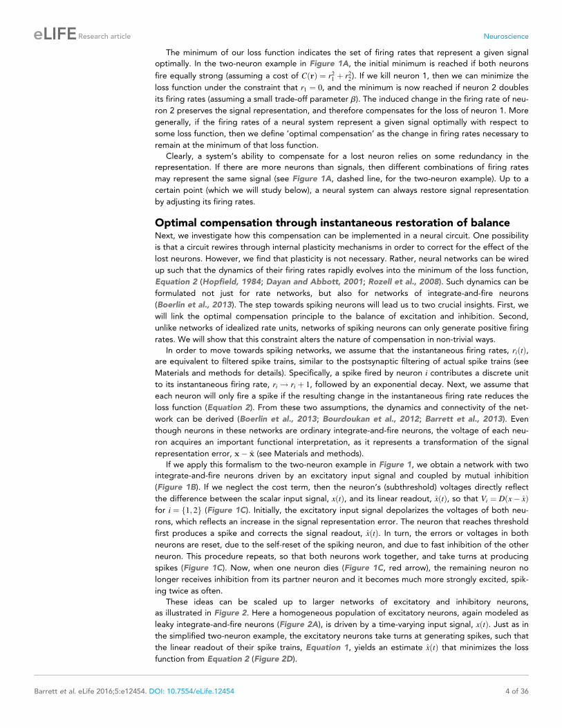
These ideas can be scaled up to larger networks of excitatory and inhibitory neurons,

as illustrated in Figure 2. Here a homogeneous population of excitatory neurons, again modeled as

leaky integrate-and-fire neurons (Figure 2A), is driven by a time-varying input signal, x tð Þ. Just as in

the simplified two-neuron example, the excitatory neurons take turns at generating spikes, such that

the linear readout of their spike trains, Equation 1, yields an estimate x tð Þ that minimizes the loss

function from Equation 2 (Figure 2D).




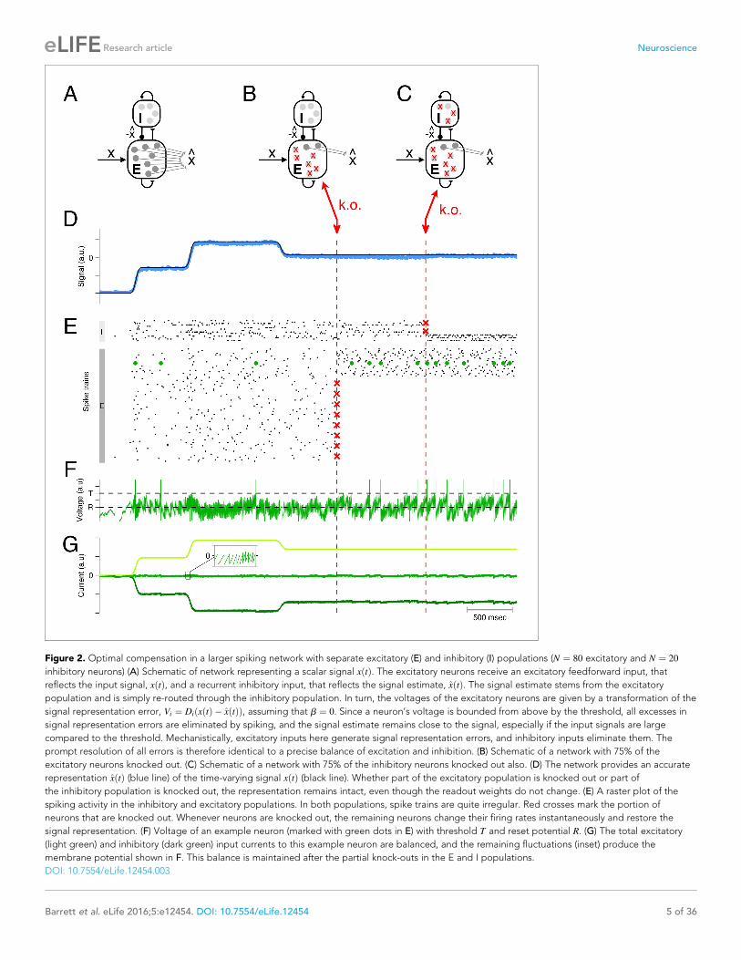
Figure 2. Optimal compensation in a larger spiking network with separate excitatory (E) and inhibitory (I) populations (N ¼ 80 excitatory and N ¼ 20

inhibitory neurons) (A) Schematic of network representing a scalar signal xðtÞ. The excitatory neurons receive an excitatory feedforward input, that

reflects the input signal, xðtÞ, and a recurrent inhibitory input, that reflects the signal estimate, xðtÞ. The signal estimate stems from the excitatory

population and is simply re-routed through the inhibitory population. In turn, the voltages of the excitatory neurons are given by a transformation of the

signal representation error, Vi ¼ DiðxðtÞ � xðtÞÞ, assuming that b ¼ 0. Since a neuron’s voltage is bounded from above by the threshold, all excesses in

signal representation errors are eliminated by spiking, and the signal estimate remains close to the signal, especially if the input signals are large

compared to the threshold. Mechanistically, excitatory inputs here generate signal representation errors, and inhibitory inputs eliminate them. The

prompt resolution of all errors is therefore identical to a precise balance of excitation and inhibition. (B) Schematic of a network with 75% of the

excitatory neurons knocked out. (C) Schematic of a network with 75% of the inhibitory neurons knocked out also. (D) The network provides an accurate

representation xðtÞ (blue line) of the time-varying signal xðtÞ (black line). Whether part of the excitatory population is knocked out or part of

the inhibitory population is knocked out, the representation remains intact, even though the readout weights do not change. (E) A raster plot of the

spiking activity in the inhibitory and excitatory populations. In both populations, spike trains are quite irregular. Red crosses mark the portion of

neurons that are knocked out. Whenever neurons are knocked out, the remaining neurons change their firing rates instantaneously and restore the

signal representation. (F) Voltage of an example neuron (marked with green dots in E) with threshold T and reset potential R. (G) The total excitatory

(light green) and inhibitory (dark green) input currents to this example neuron are balanced, and the remaining fluctuations (inset) produce the

membrane potential shown in F. This balance is maintained after the partial knock-outs in the E and I populations.

DOI: 10.7554/eLife.12454.003





Mechanistically, the excitatory population receives an excitatory input signal, x tð Þ, that is matched

by an equally strong inhibitory input. This inhibitory input is generated by a separate population of

inhibitory interneurons, and is effectively equivalent to the (re-routed) signal estimate, x tð Þ. As a

result, the (subthreshold) voltage of each excitatory neuron is once again determined by the signal

representation error, x tð Þ � x tð Þ, and a neuron will only fire when this error exceeds its (voltage)

threshold. By design, each spike improves the signal estimate, and decreases the voltages. The spike

rasters of both populations are shown in Figure 2E.

Since the signals are excitatory and the signal estimates are inhibitory, the tight tracking of the

signal by the signal estimate corresponds to a tight tracking of excitation by inhibition. The network

is therefore an example of a balanced network in which inhibition and excitation track each

other spike by spike (Deneve and Machens, 2016). Importantly, the excitatory-inhibitory (EI) balance

is a direct correlate of the signal representation accuracy (see Materials and methods for mathemati-

cal details).

Now, when some portion of the excitatory neural population is eliminated (Figure 2B), the inhibi-

tory neurons receive less excitation, and in turn convey less inhibition to the remaining excitatory

neurons. Consequently, the excitatory neurons increase their firing rates, and the levels of inhibition

(or excitation) readjust automatically such that EI balance is restored (see Figure 2G for an example

neuron). The restoration of balance guarantees that the signals continue to be represented accu-

rately (Figure 2D). This compensation happens because each excitatory neuron seeks to keep the

signal representation error in check, with or without the help of the other excitatory neurons. When

one neuron dies, the remaining excitatory neurons automatically and rapidly assume the full burden

of signal representation.

Similar principles hold when part of the inhibitory population is knocked out (Figure 2C). The

inhibitory population here is constructed to faithfully represent its ‘input signals’, which are given by

the postsynaptically filtered spike trains of the excitatory neurons. Consequently, the inhibitory pop-

ulation acts similarly to the excitatory population, and its response to neuron loss is almost identical.

When inhibitory neurons are knocked out, the remaining inhibitory neurons increase their firing rates

in order to restore the EI balance. Again, the compensation happens because each inhibitory neuron

seeks to keep its signal representation error in check, independent of the other inhibitory neurons.

The recovery boundaryNaturally, the recovery from neural loss is not unlimited. As we will show now, the resultant recovery

boundary is marked by a breakdown in the balance of excitation and inhibition. In Figure 2, this

recovery boundary coincides with a complete knock-out of either the excitatory or the inhibitory

population. The nature of the recovery boundary becomes more complex, however, if a network

tracks more than one signal.

In Figure 3 we show an example network that represents two sinusoidal signals,

x tð Þ ¼ x1 tð Þ; x2 tð Þð Þ. The spikes of each neuron contribute to two readouts, and the decoding weights

Di of the neurons correspond to two-dimensional vectors (Figure 3D). The two signals and the cor-

responding signal estimates are shown in Figure 3E, and the spike trains of the excitatory popula-

tion are shown in Figure 3F. (Here and in the following, we will focus on neuron loss in the

excitatory population only, and replace the inhibitory population by direct inhibitory connections

between excitatory neurons, see Figure 3A–C. This simplification does not affect the compensatory

properties of the network, see Materials and methods.)

When part of the excitatory population is lost (Figure 3B,D), the remaining neurons compensate

by adjusting their firing rates, and the signal representation remains intact (Figure 3E,F, first k.o.).

However, when too many cells are eliminated from the network (Figure 3C,D), some portions of the

signal can no longer be represented, no matter how the remaining neurons change their firing rates

(Figure 3E,F, second k.o.). In this example, the recovery boundary occurs when all the neurons with

negative-valued readout weights along the x1-axis have been lost, so that the network can no longer

represent the negative component of the first signal (Figure 3E, second k.o.). The representation of

signal x2 tð Þ is largely unaffected, so the deficits are only partial.

The recovery boundary is characterized by the network’s inability to correct signal representation

errors. Since the neurons’ voltages correspond to transformations of these signal representation

errors, the recovery boundary occurs when some of these voltages run out of bounds (Figure 3G,

arrows). Such aberrations of the voltages are caused by an excess of either positive or negative




Figure 3. Optimal compensation and recovery boundary in a network with N ¼ 32 excitatory neurons representing a two-dimensional signal

xðtÞ ¼ ðx1ðtÞ; x2ðtÞÞ. (A–C) Schematic of network and knock-out schedule. (Inhibitory neurons not explicitly modeled for simplicity, see text.) (B) Neural

knock-out that leads to optimal compensation. (C) Neural knock-out that pushes the system beyond the recovery boundary. (D) Readout or decoding

weights of the neurons. Since the signal is two-dimensional, each neuron contributes to the readout with two decoding weights, shown here as black

Figure 3 continued on next page




currents. Indeed, the ratio of positive to negative currents becomes disrupted after the second k.o.,

precisely when x1 tð Þ becomes negative (Figure 3H). Whereas a neuron can always ‘eliminate’ a posi-

tive, depolarizing current by spiking, it cannot eliminate any negative, hyperpolarizing currents, and

these latter currents therefore reflect signal representation errors that are not eliminated within the

network.

Here, positive currents are generated by excitatory inputs, whereas negative currents are gener-

ated by inhibitory inputs as well as the self-reset currents after an action potential. The self-reset cur-

rents become negligible in networks in which the number of neurons, N, is much larger than the

number of input signals, M (see Figure 2; see also Materials and methods). Even in Figure 3 this is

approximately the case, so that the ratio of positive to negative currents is similar to the ratio of

excitatory to inhibitory synaptic inputs (Figure 3I). The recovery boundary is then signified by a dra-

matic breakdown in the balance of excitatory and inhibitory currents.

In this simple example, the recovery boundary emerged because neurons were knocked out in a

systematic and ordered fashion (according to the features that they represented). Such a scenario

may correspond to lesions or knock-outs in systems in which neural tuning is topologically organized.

If the representational features of neurons are randomly interspersed, we find a different scenario.

Indeed, when neurons are knocked out at random in our model, the network can withstand the loss

of many more neurons. We find that signals are well represented until only a few neurons remain

(Figure 3J).

At the recovery boundary, the few remaining neurons will shoulder the full representational load.

This can easily become an unwieldy situation because the firing rates of the remaining neurons must

become unrealistically large to compensate for all the lost neurons. In reality, neural activity will satu-

rate at some point, in which case the recovery boundary occurs much earlier. For instance, we find

that the example network tolerates up to 70–80% of random neuron loss if the maximum firing rate

of a neuron is unbounded (Figure 3J), whereas it will only tolerate 40–50% of random neuron loss if

the maximum firing rate is 80 Hz (Figure 3K).

The influence of idle neurons on tuning curve shapesSo far we have considered what happens when neurons are lost permanently in a neural circuit,

either because of their death or because of experimental interventions. We have shown that net-

works can compensate for this loss up to a recovery boundary. Independent of whether compensa-

tion is successful or not, it is always marked by changes in firing rates. We will now show how to

quantify and predict these changes.

To do so, we first notice that neurons can also become inactive temporarily in a quite natural

manner. In sensory systems, for instance, certain stimuli may inhibit neurons and silence them. This

natural, temporary inactivity of neurons leads to similar, ‘compensatory’ effects on the population

level in our networks. These effects will provide important clues to understanding how neurons’ fir-

ing rates need to change whenever neurons become inactive, whether in a natural or non-natural

context.

Figure 3 continued

dots. Red crosses in the central and right panel indicate neurons that are knocked out at the respective time. (E) Signals and readouts. In this example,

the two signals (black lines) consist of a sine and cosine. The network provides an accurate representation (blue lines) of the signals, even after 25% of

the neurons have been knocked out (first dashed red line). When 50% of the neurons are knocked out (second dashed red line), the representation of

the first signal fails temporarily (red arrow). (F) A raster plot of the spiking activity of all neurons. Neurons take turns in participating in the

representation of the two signals (which trace out a circle in two dimensions), and individual spike trains are quite irregular. Red crosses mark the

portion of neurons that are knocked out. Colored neurons (green, yellow, and purple dots) correspond to the neurons with the decoder weights shown

in panel D. Note that the green and purple neurons undergo dramatic changes in firing rate after the first and second knock-outs, respectively, which

reflects their attempts to restore the signal representation. (G) Voltages of the three example neurons (marked with green, yellow, and purple dots in D

and F), with threshold T and reset potential R. (H) Ratio of positive (E; excitation) and negative (I+R; inhibition and reset) currents in the three example

neurons. After the first knock-out, the ratio remains around one, and the system remains balanced despite the loss of neurons. After the second knock-

out, part of the signal can no longer be represented, and balance in the example neurons is (temporarily) lost. (I) Ratio of excitatory and inhibitory

currents. Similar to H, except that a neuron’s self-reset current is not included. (J) When neurons are knocked out at random, the network can withstand

much larger percentages of cell loss. Individual grey traces show ten different, random knock-out schemes, and the black trace shows the average. (K)

When neurons saturate, the overall ability of the network to compensate for neuron loss decreases.

DOI: 10.7554/eLife.12454.004





For simplicity, let us focus on constant input signals, x tð Þ ¼ x, and study the average firing rates

of the neurons, �r. For constant inputs, the average firing rates must approach the minimum of the

same loss function as in Equation 2 so that,

�rðxÞ ¼ arg min�ri�0;8i

x� xð Þ2þbCð�rÞh i

(3)

where the signal estimate, x¼P

iDi�ri, is formed using the average firing rates. This minimization is

performed under the constraint that firing rates must be positive, since the firing rates of spiking

neurons are positive valued quantities, by definition. Mathematically, the corresponding optimization

problem is known as ‘quadratic programming’ (see Materials and methods for more details). Tradi-

tionally, studies of population coding or efficient coding assume both positive and negative firing

rates (Dayan and Abbott, 2001; Olshausen and Field, 1996; Simoncelli and Olshausen, 2001),

and the restriction to positive firing rates is generally considered an implementational problem

(Rozell et al., 2008). Surprisingly, however, we find that the constraint changes the nature of the sol-

utions and provides fundamental insights into the shapes of tuning curves in our networks, as clari-

fied below.

An example is shown in Figure 4 where we focus on networks of increasing complexity that rep-

resent two signals. For simplicity, we keep the second signal constant (‘fixed background’ signal,

x2 ¼ rB) and study the firing rates of all neurons as a function of the first signal, x1 ¼ x. Solving Equa-

tion 3 for a range of values, we obtain N neural tuning curves, �r x1ð Þ ¼ r1 x1ð Þ; r2 x1ð Þ; . . .ð Þ (Figure 4,

second column). These tuning curves closely match those measured in simulations of the corre-

sponding spiking networks (Figure 4, third and fourth column; see supplementary materials for

mathematical details).

We observe that the positivity constraint produces non-linearities in neural tuning curves. We illus-

trate this using a two-neuron system with two opposite-valued readout weights for the first signal

(Figure 4A, first column). At signal value x ¼ 0, both neurons fire at equal rates so that the readout

x, Equation 1, correctly becomes x / �r1 � �r2ð Þ ¼ 0. When we move to higher values of x, the firing

rate of the first neuron, �r1, increases linearly (Figure 4A, second column, orange line), and the firing

rate of the second neuron, �r2, decreases linearly (Figure 4A, second column, blue line), so that in

each case, x» x. Eventually, around x ¼ 0:4, the firing rate of neuron two hits zero (Figure 4A, black

arrow). At this point, neuron two has effectively disappeared from the network. Since it cannot

decrease below zero, and because the estimated value x must keep growing with x, the firing rate of

neuron one must grow at a faster rate. This causes a kink in its tuning curve (Figure 4A, black arrow).

This kink in the tuning curve slope is an indirect form of optimal compensation, where the network is

compensating for the temporary silencing of a neuron.

More generally, the firing rates of neurons are piecewise linear functions of the input signals. In

Figure 4B,C, every time one of the neurons hits the zero firing rate lower bound, the tuning curve

slopes of all the other neurons change. We furthermore note that the tuning curves also depend on

the form of the cost terms, C �rð Þ. If there is no cost term, there are many equally favorable firing rate

combinations that produce identical readouts (Figure 1A). The precise choice of a cost term deter-

mines which of these solutions is found by the network. We provide further geometric insights into

the shape of the tuning curves obtained in our networks in Figure 4—figure supplements 1–3 and

in the Materials and methods.

Tuning curves before and after neuronal silencingWe can now calculate how tuning curves change shape in our spiking network following neuronal

loss. When a set of neurons are killed or silenced within a network, their firing rates are effectively

set to zero. We can include this silencing of neurons in our loss function by simply clamping the

respective neurons’ firing rates to zero:

�r xð Þ ¼ arg min�ri�0 if i2X

�rj¼0 if j2Y

x� xð Þ2þbC �rð Þh i

(4)

where X denotes the set of healthy neurons and Y the set of dead (or silenced) neurons. This addi-

tional clamping constraint is the mathematical equivalent of killing neurons. In turn, we can study the




tuning curves of neurons in networks with knocked-out neurons without having to simulate the corre-

sponding spiking networks every single time.

As a first example, we revisit the network shown in Figure 4C, which represents a signal x1 ¼ x,

and a constant ‘background’ signal x2 ¼ rB. This network exhibits a complex mixture of tuning

curves, i.e., firing rates as a function of the primary signal x1 ¼ x, with positive and negative slopes,

and diverse threshold crossings (Figure 5B). When we knock out a subset of neurons (Figure 5A,

Figure 4. Explaining tuning curves in the spiking network with quadratic programming. (A) A network with N ¼ 2 neurons. The first column shows the

decoding weights for the two neurons. The first decoding weight determines the readout of the signal x1 ¼ x, whereas the second decoding weight

helps to represent a constant background signal x2 ¼ rB. The second column shows the tuning curves, i.e., firing rates as a function of x, predicted

using quadratic programming. The third column shows the tuning curves measured during a 1 s simulation of the respective spiking network. The

fourth column shows the match between the measured and predicted tuning curves. (B) Similar to A , but using a network of N ¼ 16 neurons with

inhomogeneous, regularly spaced decoding weights. The resulting tuning curves are regularly spaced. Neurons with small decoding weight magnitude

have eccentric firing rate thresholds and shallow slopes; neurons with large decoding weight magnitudes have central firing rate thresholds and steep

slopes. (C) Similar to B except that decoding weights and cost terms are irregularly spaced. This irregularity leads to inhomogeneity in the balanced

network tuning curves, and in the quadratic programming prediction (see also Figure 4—figure supplements 1–3).

DOI: 10.7554/eLife.12454.005

The following figure supplements are available for figure 4:

Figure supplement 1. The geometry of quadratic programming.

DOI: 10.7554/eLife.12454.006

Figure supplement 2. A taxonomy of tuning curve shapes.

DOI: 10.7554/eLife.12454.007

Figure supplement 3. Quadratic programming firing rate predictions compared to spiking network measurements.

DOI: 10.7554/eLife.12454.008








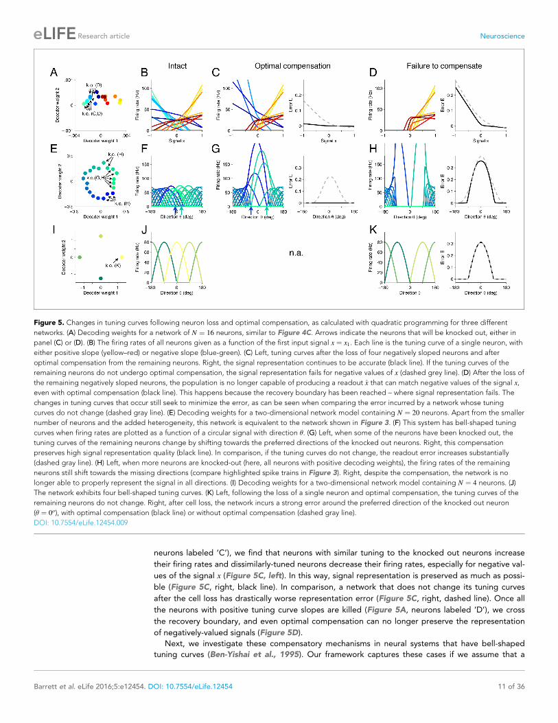
neurons labeled ‘C’), we find that neurons with similar tuning to the knocked out neurons increase

their firing rates and dissimilarly-tuned neurons decrease their firing rates, especially for negative val-

ues of the signal x (Figure 5C, left). In this way, signal representation is preserved as much as possi-

ble (Figure 5C, right, black line). In comparison, a network that does not change its tuning curves

after the cell loss has drastically worse representation error (Figure 5C, right, dashed line). Once all

the neurons with positive tuning curve slopes are killed (Figure 5A, neurons labeled ‘D’), we cross

the recovery boundary, and even optimal compensation can no longer preserve the representation

of negatively-valued signals (Figure 5D).

Next, we investigate these compensatory mechanisms in neural systems that have bell-shaped

tuning curves (Ben-Yishai et al., 1995). Our framework captures these cases if we assume that a

Figure 5. Changes in tuning curves following neuron loss and optimal compensation, as calculated with quadratic programming for three different

networks. (A) Decoding weights for a network of N ¼ 16 neurons, similar to Figure 4C. Arrows indicate the neurons that will be knocked out, either in

panel (C) or (D). (B) The firing rates of all neurons given as a function of the first input signal x ¼ x1. Each line is the tuning curve of a single neuron, with

either positive slope (yellow–red) or negative slope (blue-green). (C) Left, tuning curves after the loss of four negatively sloped neurons and after

optimal compensation from the remaining neurons. Right, the signal representation continues to be accurate (black line). If the tuning curves of the

remaining neurons do not undergo optimal compensation, the signal representation fails for negative values of x (dashed grey line). (D) After the loss of

the remaining negatively sloped neurons, the population is no longer capable of producing a readout x that can match negative values of the signal x,

even with optimal compensation (black line). This happens because the recovery boundary has been reached – where signal representation fails. The

changes in tuning curves that occur still seek to minimize the error, as can be seen when comparing the error incurred by a network whose tuning

curves do not change (dashed gray line). (E) Decoding weights for a two-dimensional network model containing N ¼ 20 neurons. Apart from the smaller

number of neurons and the added heterogeneity, this network is equivalent to the network shown in Figure 3. (F) This system has bell-shaped tuning

curves when firing rates are plotted as a function of a circular signal with direction �. (G) Left, when some of the neurons have been knocked out, the

tuning curves of the remaining neurons change by shifting towards the preferred directions of the knocked out neurons. Right, this compensation

preserves high signal representation quality (black line). In comparison, if the tuning curves do not change, the readout error increases substantially

(dashed gray line). (H) Left, when more neurons are knocked-out (here, all neurons with positive decoding weights), the firing rates of the remaining

neurons still shift towards the missing directions (compare highlighted spike trains in Figure 3). Right, despite the compensation, the network is no

longer able to properly represent the signal in all directions. (I) Decoding weights for a two-dimensional network model containing N ¼ 4 neurons. (J)

The network exhibits four bell-shaped tuning curves. (K) Left, following the loss of a single neuron and optimal compensation, the tuning curves of the

remaining neurons do not change. Right, after cell loss, the network incurs a strong error around the preferred direction of the knocked out neuron

(� ¼ 0o), with optimal compensation (black line) or without optimal compensation (dashed gray line).

DOI: 10.7554/eLife.12454.009





network represents circular signals embedded in a two-dimensional space, x ¼ cos �ð Þ; sin �ð Þð Þ, where� is the direction of our signal. To do so, we construct a network in which the decoding weights of

the neurons are spaced around a circle, with some irregularity added (Figure 5E). As a result, we

obtain an irregular combination of bell-shaped tuning curves (Figure 5F), similar to those found in

the primary visual or primary motor cortex, with each neuron having a different preferred direction

and maximum firing rate as determined by the value of the decoding weights. We note that, apart

from the smaller number of neurons and the greater irregularity of the decoding weights, this net-

work is similar to the spiking network investigated in Figure 3.

If we now kill neurons within a specific range of preferred directions (Figure 5E), then the remain-

ing neurons with the most similar directions increase their firing rates and shift their tuning curves

towards the preferred directions of the missing neurons (Figure 5G, left). Furthermore, neurons fur-

ther away from the knocked-out region will slightly skew their tuning curves by decreasing their firing

rates for directions around zero (Figure 5F,G, arrows). Overall, the portion of space that is under-

represented following cell loss becomes populated by neighboring neurons, which thereby counter-

act the loss. In turn, the signal representation performance of the population is dramatically

improved following optimal compensation compared to a system without compensatory mecha-

nisms (Figure 5G, right). Once all neurons with positive read-out weights along the first axis are

killed, the network can no longer compensate, and signal representation fails, despite the strong

changes in firing rates of the neurons (Figure 5H). This latter scenario is equivalent to the one we

observed in Figure 3 after the second knock-out.

The ability of the system to compensate for the loss of neurons depends on the redundancy of its

representation (although redundancy alone is not sufficient for compensation). If our network con-

sists of only four neurons with equally spaced readout weights (Figure 5I), then it cannot compen-

sate for the loss of neurons. Rather, we find that this model system crosses the recovery boundary

following the loss of a single neuron, and so, optimal compensation does not produce any changes

in the remaining neurons (Figure 5K, left). It occurs because the four neurons exactly partition the

four quadrants of the signal space, and the remaining neurons cannot make any changes that would

improve the signal representation.

Comparison to experimental dataDoes optimal compensation happen in real neural systems? Our framework makes strong predic-

tions for how firing rates should change following neuronal knock-outs. Unfortunately, there is cur-

rently little data on how neural firing rates change directly after the loss of neurons in a given

system. However, we found data from three systems—the oculomotor integrator in the hindbrain,

the cricket cercal system, and the primary visual cortex—which allows us to make a first comparison

of our predictions to reality. We emphasize that a strict test of our theory is left for future work.

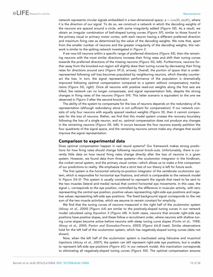
The first system is the horizontal velocity-to-position integrator of the vertebrate oculomotor sys-

tem, which is responsible for horizontal eye fixations, and which is comparable to the network model

in Figure 5A–D. This system is usually considered to represent the signals that need to be sent to

the two muscles (lateral and medial rectus) that control horizontal eye movements. In this case, the

signal x1 corresponds to the eye position, controlled by the difference in muscular activity, with zero

representing the central eye position, positive values representing right-side eye positions and nega-

tive values representing left-side eye positions. The fixed background signal corresponds to the net

sum of the two muscle activities, which we assume to remain constant for simplicity.

We find that the tuning curves of neurons measured in the right half of the oculomotor system

(Aksay et al., 2000) (Figure 6A) are similar to the positively-sloped tuning curves in our network

model calculated using Equation 3 (Figure 6B). In both cases, neurons that encode right-side eye

positions have positive slopes, and these follow a recruitment order, where neurons with shallow tun-

ing curve slopes become active before neurons with steep tuning curve slopes (Fuchs et al., 1988;

Aksay et al., 2000; Pastor and Gonzalez-Forero, 2003) (Figure 6A,B inset). Similar observations

hold for the left half of the oculomotor system, which has negatively-sloped tuning curves (data not

shown).

Now, when the left half of the oculomotor system is inactivated using lidocaine and muscimol

injections (Aksay et al., 2007), the system can still represent right-side eye positions, but is unable

to represent left-side eye positions (Figure 6C). In our network model, this inactivation corresponds

to eliminating all negatively-sloped tuning curves (Figure 5D). The optimal compensation ensures




Figure 6. Tuning curves and inactivation experiments in the oculomotor integrator of the goldfish, and in the cricket cercal system. (A) Tuning curve

measurements from right-side oculomotor neurons (Area 1 of goldfish). Firing rate measurements above 5 Hz are fit with a straight line fn ¼ knðx� Eth;nÞ,where fn is the firing rate of the nth neuron, Eth;n is the firing rate threshold, kn is the firing rate slope and x is the eye position. As the eye position

increases, from left to right, a recruitment order is observed, where neuron slopes increase as the firing rate threshold increases (inset).

Figure 6A has been adapted with permission from The American Physiological Society (Ó copyright The American Physiological Society, 2000. All

Rights Reserved).

(B) Tuning curves from our network model. We use the same parameters as in previous figures (Figure 5A), and fit the threshold-linear model to the

simulated tuning curves (Figure 5B) using the same procedure as in the experiments from Aksay et al. (2000). As in the data, a recruitment order is

observed with slopes increasing as the firing threshold increases (inset). (C) Eye position drift measurements after the pharmacological inactivation of

left side neurons in goldfish. Inactivation was performed using lidocaine and muscimol injections. Here DD ¼ Dafter � Dbefore, where Dbefore is the average

drift in eye position before pharmacological inactivation and is the average drift in eye position after pharmacological inactivation. Averages are

calculated across goldfish.

Figure 6C has been adapted with permission from McMillan Publisher Ltd: Nature Neuroscience (Ó copyright McMillan Publisher Ltd: Nature

Neuroscience, 2007. All Rights Reserved).





that the right part of the signal is still correctly represented, but the left part can no longer be repre-

sented due to the lack of negatively tuned neurons (Figure 5D and Figure 6D). Hence, these meas-

urements are consistent with our optimal compensation and recovery boundary predictions.

The second system is a small sensory system called the cricket (or cockroach) cercal system, which

represents wind velocity (Theunissen and Miller, 1991), and which is comparable to the network

model in Figure 5I–K. In the case of the cercal system, � is the wind-direction. The tuning curves we

obtain are similar to those measured, with each neuron having a different, preferred wind direction

(Theunissen and Miller, 1991), see Figure 6E. The similarity between measured tuning curves

(Figure 6E) and predicted tuning curves (Figure 5J) suggests that we can interpret cercal system

neurons to be optimal for representing wind direction using equally spaced readout weights.

When one neuron in the cercal system is killed, the remaining neurons do not change their firing

rates (Libersat and Mizrahi, 1996; Mizrahi and Libersat, 1997), see Figure 6F. This is analogous to

our predictions (Figure 5K). Indeed, our model of the cercal system has no redundancy (see

Materials and methods for more details). The cercal system in all its simplicity is therefore a nice

example of a system that exists on the ‘edge’ of the recovery boundary.

A high-dimensional example: optimal compensation in V1The relatively simple models we have described so far are useful for understanding the principle of

optimal compensation, but they are unlikely to capture the complexity of large neural populations in

the brain. Even though the network model in Figure 5E–G resembles common network models for

the primary visual or primary motor cortex, it does not capture the high-dimensional nature of repre-

sentations found in these areas. To investigate the compensatory mechanisms in more complex net-

works, we make a final generalization to systems that can represent high-dimensional signals, and

for concreteness we focus on the (primary) visual cortex, which is our third test system.

The visual cortex is generally thought to construct representations of images consisting of many

pixel values (Figure 7A). The tuning of V1 simple cells, for instance, can largely be accounted for by

assuming that neural firing rates provide a sparse code of natural images (Olshausen and Field,

1996; Simoncelli and Olshausen, 2001). In accordance with this theory, we choose a model that

represents image patches (size 12� 12, corresponding to M ¼ 144 dimensions), and we use decod-

ing weights that are optimized for natural images (see Materials and methods). Neurons in this

model are tuned to both the orientation and polarity of edge-like images (Figure 7D), where the

polarity is either a bright edge with dark flanks, or the opposite polarity – a dark edge with bright

flanks. Orientation tuning emerges because natural images typically contain edges at many different

orientations, and a sparse code captures these natural statistics (Olshausen and Field, 1996;

Simoncelli and Olshausen, 2001). Polarity tuning emerges as a natural consequence of the positivity

constraint, because a neuron with a positive firing rate cannot represent edges at two opposing

polarities. Similar polarity tuning has been obtained before, but with an additional constraint that

decoding weights be strictly positive (Hoyer, 2003, 2004).

As before, we compute the firing rates of our neural population by solving Equation 3, which

provides a convenient approximation of the underlying spiking network. We then silence all neurons

with a vertical orientation preference (Figure 7E) and calculate the resulting changes in firing rates

Figure 6 continued

(D) Eye position representation error of the model network following optimal compensation. Here DE ¼ EC � EI , where is the representation error of

the intact system and EC is the representation error following optimal compensation. These representation errors are calculated using the loss function

from Equation 2 . (E) Firing rate recordings from the cricket cercal system in response to air currents from different directions. Each neuron has a

preference for a different wind direction. Compare with Figure 5J.

Figure 6E has been adapted with permission from The American Physiological Society (Ó copyright The American Physiological Society, 1991. All

Rights Reserved).

(F) Measured change of cockroach cercal system tuning curves following the ablation of another cercal system neuron. In all cases, there is no

significant change in firing rate. This is consistent with the lack of compensation in Figure 5K. The notation GI2-GI3 denotes that Giant Interneuron 2 is

ablated and the change in Giant Interneuron 3 is measured. The firing rate after ablation is given as a percentage of the firing rate before ablation.

Figure 6F has been adapted with permission from The American Physiological Society (Ó copyright The American Physiological Society, 1997. All

Rights Reserved).

DOI: 10.7554/eLife.12454.010





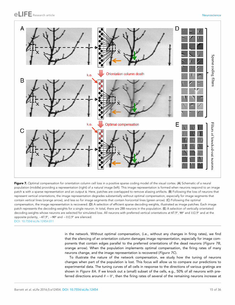
in the network. Without optimal compensation, (i.e., without any changes in firing rates), we find

that the silencing of an orientation column damages image representation, especially for image com-

ponents that contain edges parallel to the preferred orientations of the dead neurons (Figure 7B,

orange arrow). When the population implements optimal compensation, the firing rates of many

neurons change, and the image representation is recovered (Figure 7C).

To illustrate the nature of the network compensation, we study how the tuning of neurons

changes when part of the population is lost. This focus will allow us to compare our predictions to

experimental data. The tuning curves of all cells in response to the directions of various gratings are

shown in Figure 8A. If we knock out a (small) subset of the cells, e.g., 50% of all neurons with pre-

ferred directions around � ¼ 0�, then the firing rates of several of the remaining neurons increase at

Figure 7. Optimal compensation for orientation column cell loss in a positive sparse coding model of the visual cortex. (A) Schematic of a neural

population (middle) providing a representation (right) of a natural image (left). This image representation is formed when neurons respond to an image

patch x with a sparse representation and an output x. Here, patches are overlapped to remove aliasing artifacts. (B) Following the loss of neurons that

represent vertical orientations, the image representation degrades substantially without optimal compensation, especially for image segments that

contain vertical lines (orange arrow), and less so for image segments that contain horizontal lines (green arrow). (C) Following the optimal

compensation, the image representation is recovered. (D) A selection of efficient sparse decoding weights, illustrated as image patches. Each image

patch represents the decoding weights for a single neuron. In total, there are 288 neurons in the population. (E) A selection of vertically orientated

decoding weights whose neurons are selected for simulated loss. All neurons with preferred vertical orientations at 67:5o, 90o and 112:5o and at the

opposite polarity, �67:5o, �90o and �112:5o are silenced.

DOI: 10.7554/eLife.12454.011





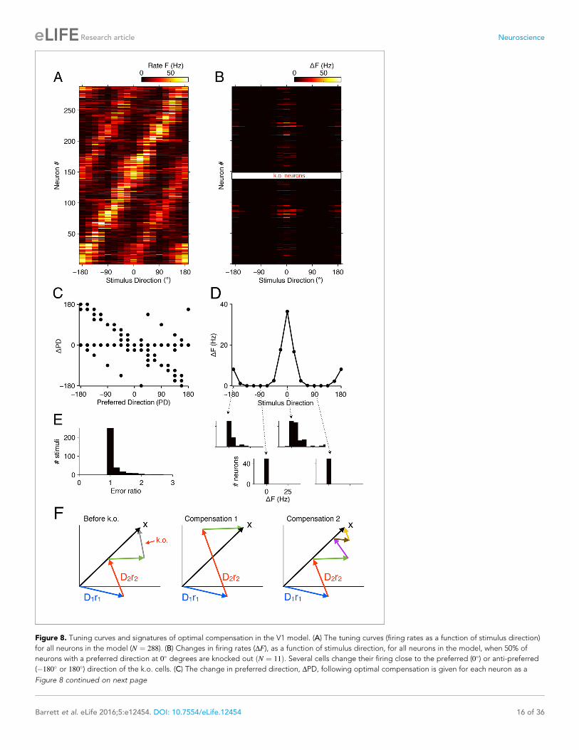
Figure 8. Tuning curves and signatures of optimal compensation in the V1 model. (A) The tuning curves (firing rates as a function of stimulus direction)

for all neurons in the model (N ¼ 288). (B) Changes in firing rates (DF), as a function of stimulus direction, for all neurons in the model, when 50% of

neurons with a preferred direction at 0� degrees are knocked out ðN ¼ 11Þ. Several cells change their firing close to the preferred (0�) or anti-preferred

(�180� or 180�) direction of the k.o. cells. (C) The change in preferred direction, DPD, following optimal compensation is given for each neuron as a





the preferred direction of the silenced cells (Figure 8B,D). As a consequence, the preferred direc-

tions of many cells shift toward the preferred direction of the silenced cells (Figure 8C). Unlike the

simple example in Figure 5G, however, these shifts occur in neurons throughout the population,

and not just in neurons with neighboring directions. For the affected stimuli, the shifts decrease the

representation errors compared to a system without compensation (Figure 8E).

The more complicated pattern of firing rate changes occurs for two reasons. First, neurons repre-

sent more than the direction of a grating—they represent a 12 � 12 image patch, i.e., a vector in a

high-dimensional space (Figure 8F). Such a vector will generally be represented by the firing of

many different neurons, each of which contributes with its decoding vector, Di, weighted by its firing

rate, ri. However, these neurons will rarely point exactly in the right (stimulus) direction, and only

their combined effort allows them to represent the stimulus. When some of the neurons contributing

to this stimulus representation are knocked out, the network will recruit from the pool of all neurons

whose decoding vectors are non-orthogonal to the stimulus vector. In turn, each of these remaining

neurons gets assigned a new firing rate such that the cost term in Equation 2 is minimized. Second,

high-dimensional spaces literally provide a lot of space. Whereas stacking 20 neurons in a two-

dimensional space (as in Figure 5E,F) immediately causes crowding, with neighboring neurons shar-

ing a substantial overlap of information, stacking e.g. 1000 neurons in a 100-dimensional space

causes no such thing. Rather, neurons can remain almost independent, while sharing only small

amounts of information. As a consequence, not a single pair of the naturally trained decoding

weights in our model will point in similar directions. In other words, when we knock out a set of neu-

rons, there are no similarly tuned neurons that could change their firing rates in order to restore the

representation. Rather, the compensation for a single lost neuron will require the concerted effort of

several other neurons, and many of the required changes can be small and subtle. However, all of

these changes will seek to restore the lost information, and cells will shift their tuning towards that

of the lost neurons.

As a consequence of this additional complexity, we find that firing rates at the anti-preferred

direction also increase (Figure 8B,D). A key reason for this behavior is that many neurons are

strongly tuned to orientation, but only weakly tuned to direction, so that eliminating neurons with 0�

degree direction preference also eliminates some of the representational power at the anti-preferred

direction.

Finally, although our model is simply a (positive) sparse coding model, we note that most of its

predictions are consistent with experiments in the cat visual cortex, in which sites with specific orien-

tation or direction tuning are silenced using GABA (Crook et al., 1996, 1997, 1998) (Figure 9 and

Figure 9—figure supplement 1), while recording the firing rates of nearby neurons. Neurons that

escape silencing in the cat visual cortex also shift their tuning curves towards the preferred directions

of the silenced neurons (Figure 9A). More specifically, three types of changes were found: (1) Neu-

rons whose preferred direction was different to that of the silenced neurons (PD>22:5�) will increasetheir firing rates at the knocked-out direction and broaden their tuning (see Figure 9A, top row for

an example). (2) Neurons whose preferred direction was opposite to the silenced neurons will

Figure 8 continued

function of its preferred direction before cell loss. Many cells shift their preferred direction towards the preferred direction of the knocked out cells. (D)

The average change in firing rate due to optimal compensation (DF) is calculated at each stimulus direction, where the average is taken across the

neural population in B. There is a substantial increase in firing rates close to the preferred directions of the knocked out cells. The histograms on the

bottom show the firing rate changes in the population as a function of four different stimulus directions. Stimuli with horizontal orientations (0� or

�180�) lead to firing rate changes, but stimuli with vertical orientations ( �90

�) do not. (E) Ratio of reconstruction errors (no compensation vs. optimal

compensation) across a large range of Gabor stimuli. For most stimuli, no compensation is necessary, but for a few stimuli (mostly those showing edges

with horizontal orientations) the errors are substantially reduced if the network compensates. (F) Schematic of compensation in high-dimensional

spaces. In the intact state (left), a stimulus (black arrow) is represented through the firing of four neurons (colored arrows, representing the decoding

vectors of the neurons, weighted by their firing rates). If the grey neuron is knocked out, one possibility to restore the representation may be to modify

the firing rates of the remaining neurons (center). However, in higher-dimensional spaces, the three remaining arrows will not be sufficient to reach any

stimulus position, so that this possibility is usually ruled out. Rather, additional neurons will need to be recruited (right) in order to restore the stimulus

representation. These neurons may have contributed only marginally (or not at all) to the initial stimulus representation, because their contribution was

too costly. In the absence of the grey neuron, however, they have become affordable. If no combination of neurons allows the system to reach the

stimulus position, then the recovery boundary has been crossed.

DOI: 10.7554/eLife.12454.012





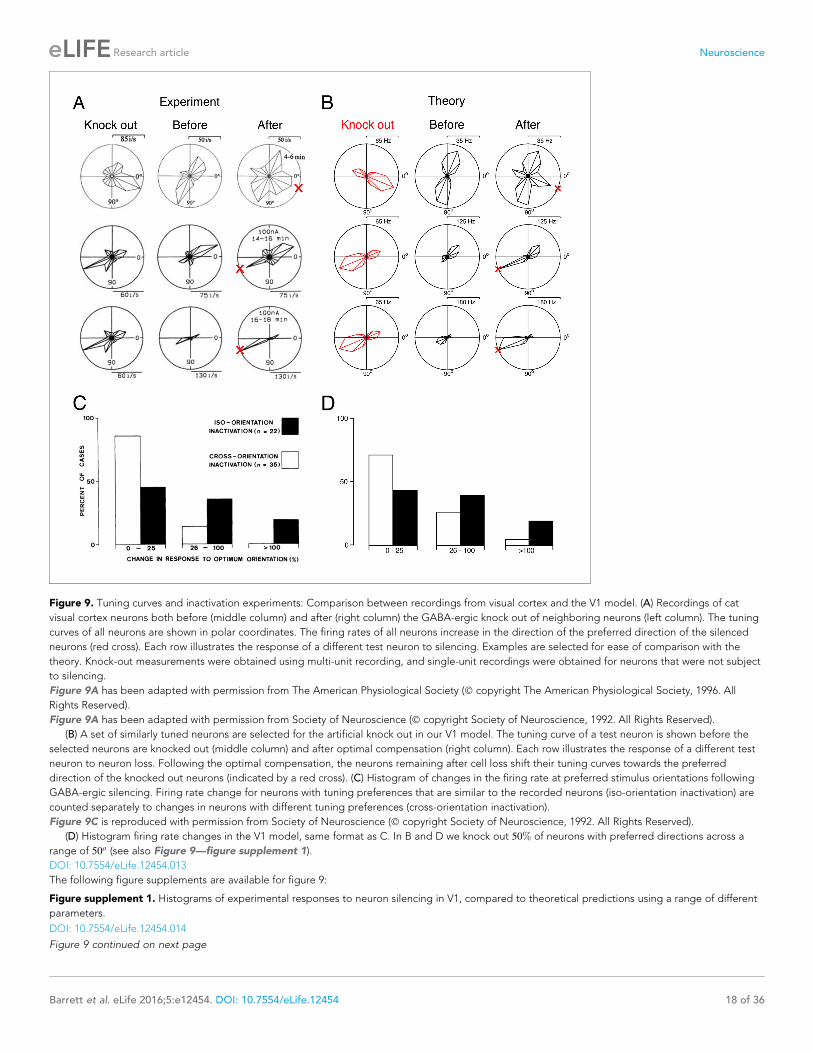
Figure 9. Tuning curves and inactivation experiments: Comparison between recordings from visual cortex and the V1 model. (A) Recordings of cat

visual cortex neurons both before (middle column) and after (right column) the GABA-ergic knock out of neighboring neurons (left column). The tuning

curves of all neurons are shown in polar coordinates. The firing rates of all neurons increase in the direction of the preferred direction of the silenced

neurons (red cross). Each row illustrates the response of a different test neuron to silencing. Examples are selected for ease of comparison with the

theory. Knock-out measurements were obtained using multi-unit recording, and single-unit recordings were obtained for neurons that were not subject

to silencing.

Figure 9A has been adapted with permission from The American Physiological Society (Ó copyright The American Physiological Society, 1996. All

Rights Reserved).

Figure 9A has been adapted with permission from Society of Neuroscience (Ó copyright Society of Neuroscience, 1992. All Rights Reserved).

(B) A set of similarly tuned neurons are selected for the artificial knock out in our V1 model. The tuning curve of a test neuron is shown before the

selected neurons are knocked out (middle column) and after optimal compensation (right column). Each row illustrates the response of a different test

neuron to neuron loss. Following the optimal compensation, the neurons remaining after cell loss shift their tuning curves towards the preferred

direction of the knocked out neurons (indicated by a red cross). (C) Histogram of changes in the firing rate at preferred stimulus orientations following

GABA-ergic silencing. Firing rate change for neurons with tuning preferences that are similar to the recorded neurons (iso-orientation inactivation) are

counted separately to changes in neurons with different tuning preferences (cross-orientation inactivation).

Figure 9C is reproduced with permission from Society of Neuroscience (Ó copyright Society of Neuroscience, 1992. All Rights Reserved).

(D) Histogram firing rate changes in the V1 model, same format as C. In B and D we knock out 50% of neurons with preferred directions across a

range of 50o (see also Figure 9—figure supplement 1).

DOI: 10.7554/eLife.12454.013

The following figure supplements are available for figure 9:

Figure supplement 1. Histograms of experimental responses to neuron silencing in V1, compared to theoretical predictions using a range of different

parameters.

DOI: 10.7554/eLife.12454.014







increase their firing rates towards the knocked out direction (see Figure 9A, middle row for an

example). (3) Neurons whose preferred direction was similar to the silenced neurons (PD<22:5�) willeither increase their firing to the knocked out direction (see Figure 9A, bottom row) or decrease

their firing to the knocked out direction (data not shown).

In our sparse coding model, we find increases in firing rates to the knocked-out directions in all

three types of neurons (with different direction preference, opposite direction preference, or similar

direction preference), see Figure 9B. We do not observe a decrease in firing to the knocked-out

directions. While this mismatch likely points towards the limits of our simplified model (which models

a relatively small set of simple cells) in comparison with the data (which examines both simple and

complex cells in both V1 and V2), it does not violate the optimal compensation principle. Due to the

complexity of interactions in a high-dimensional space, a decrease in firing of a few neurons to the

missing directions is not a priori ruled out in our model, as long as there is a net increase to the miss-

ing directions across the whole population. Indeed, when increasing the redundancy in our V1 model

(e.g. by moving from N ¼ 288 neurons to N ¼ 500 neurons while keeping the dimensionality of the

stimulus fixed), we find that several neurons start decreasing their firing rates in response to the

knocked-out directions, even though the average firing rate changes in the population remain posi-

tive (data not shown).

We emphasize that there are only a few free parameters in our model. Since the decoding

weights are learnt from natural images using the (positive) sparse coding model, we are left with the

dimensionality of the input space, the number of neurons chosen, and the number of neurons

knocked out. The qualitative results are largely independent of these parameters. For instance, the

precise proportion of neurons knocked out in the experimental studies (Crook and Eysel, 1992) is

not known. However, for a range of reasonable parameter choices (50–75% knock out of all neurons

with a preferred direction), our predicted tuning curve changes are consistent with the recorded

population response to neuron silencing (Crook and Eysel, 1992) (Figure 9—figure supplement

1B). Furthermore, if we increase the redundancy of the system by scaling up the number of neurons,

but not the number of stimulus dimensions, we shift the recovery boundary to a larger fraction of

knocked-out neurons, but we do not change the nature of the compensatory response (Figure 9—

figure supplement 2A,B). At high degrees of redundancy (or so-called ‘over-completeness’), quanti-

tive fluctuations in tuning curve responses are averaged out, indicating that optimal compensation

becomes invariant to over-completeness (Figure 9—figure supplement 2C,D). Given the few

assumptions that enter our model, we believe that the broad qualitative agreement between our

theory and the data is quite compelling.

DiscussionTo our knowledge, optimal compensation for neuron loss has not been proposed before. Usually,

cell loss or neuron silencing is assumed to be a wholly destructive action, and the immediate neural

response is assumed to be pathological, rather than corrective. Synaptic plasticity is typically given

credit for the recovery of neural function. For example, synaptic compensation has been proposed

as a mechanism for memory recovery following synaptic deletion (Horn et al., 1996), and optimal

adaptation following perturbations of sensory stimuli (Wainwright, 1999) and motor targets

(Shadmehr et al., 2010; Braun et al., 2009; Kording et al., 2007) has also been observed, but on a

slow time scale consistent with synaptic plasticity. In this work, we have explored the properties of

an instantaneous, optimal compensation, that can be implemented without synaptic plasticity, on a

much faster time scale, through balanced network dynamics.

Our work is built upon a connection between two separate theories: the theory of balanced net-

works, which is widely regarded to be the standard model of cortical dynamics (van Vreeswijk and

Sompolinsky, 1996, 1998; Amit and Brunel, 1997; Renart et al., 2010; Deneve and Machens,

2016) and the theory of efficient coding, which is arguably our most influential theory of neural com-

putation (Barlow, 1961; Salinas, 2006; Olshausen and Field, 1996; Bell and Sejnowski, 1997;

Figure 9 continued

Figure supplement 2. Optimal compensation in V1 models with different degrees of redundancy or over-completeness.

DOI: 10.7554/eLife.12454.015





Greene et al., 2009). This connection relies on the following two derivations: (1) We derive a tightly

balanced spiking network from a quadratic loss function, following the recent work of (Boerlin et al.,

2013; Boerlin and Deneve, 2011) by focusing on the part of their networks that generate a spike-

based representation of the information. (2) We show that the firing rates in these spiking networks

also obey a quadratic loss function, albeit with a positivity constraint on the firing rate

(Barrett et al., 2013). This constrained minimization problem, called quadratic programming, pro-

vides a novel link between spiking networks and firing rate calculations. While the importance of

positivity constraints has been noted in other contexts (Lee and Seung, 1999; Hoyer, 2003,

2004; Salinas, 2006), here we show its dramatic consequences in shaping tuning curves, which had

not been appreciated previously. In turn, we obtain a single normative explanation for the polarity

tuning of simple cells (Figure 7D), tuning curves in the oculomotor system (Figure 6A,B), and tuning

curves in the cricket cercal system (Figure 6E), as well as the mechanisms underlying the generation

of these tuning curves, and the response of these systems to neuron loss.

Several alternative network models have been proposed that minimize similar loss functions as in

our work (Dayan and Abbott, 2001; Rozell et al., 2008; Hu et al., 2012; Charles et al., 2012;

Druckmann and Chklovskii, 2012). However, in all these models, neurons produce positive and

negative firing rates (Dayan and Abbott, 2001; Rozell et al., 2008; Charles et al., 2012;

Druckmann and Chklovskii, 2012), or positive and negative valued spikes (Hu et al., 2012). The

compensatory response of these systems will be radically different, because oppositely tuned neu-

rons can compensate for each other by increasing their firing rates and changing sign, which is

impossible in our networks. Similar reasoning holds for any efficient coding theories that assume

positive and negative firing rates.

Whether general spiking networks support some type of compensation will depend on the specif-

ics of their connectivity (see Materials and methods). For instance, spiking networks that learn to effi-

ciently represent natural images could potentially compensate for neuron loss (Zylberberg et al.,

2011; King et al., 2013). Furthermore, networks designed to generate EI balance through strong

recurrent dynamics will automatically restore balance when neurons are lost (van Vreeswijk and

Sompolinsky, 1996, 1998; Amit and Brunel, 1997; Renart et al., 2010). In turn, networks whose

representations and computations are based on such randomly balanced networks may be able to

compensate for neuron loss as well (Vogels et al., 2011; Hennequin et al., 2014), as has been

shown for neural integrators (Lim and Goldman, 2013). However, the optimality or the speed of the

compensation is likely to increase with the tightness of the balancing. In turn, the tightness of EI bal-

ance is essentially determined by synaptic connectivity, whether through experience-dependent

learning of the synaptic connections (Haas et al., 2006; Vogels et al., 2011; Bourdoukan et al.,

2012; Luz and Shamir, 2012), through scaling laws for random connectivities (van Vreeswijk and

Sompolinsky, 1996, 1998; Amit and Brunel, 1997; Renart et al., 2010), or by design, via the

decoding weights of linear readouts, as in our case (Boerlin et al., 2013; Barrett et al., 2013).

Future work may resolve the commonalities and differences of these approaches.

The principle of optimal compensation is obviously an idealization, and any putative compensa-

tory mechanism of an actual neural system may be more limited. That said, we have catalogued a

series of experiments in which pharmacologically induced changes in neural activities and in behavior

can be explained in terms of optimal compensation. These experiments were not originally con-

ducted to test any specific compensatory mechanisms, and so, the results of each individual experi-

ment were explained by separate, alternative mechanisms (Aksay et al., 2007; Goncalves et al.,

2014; Libersat and Mizrahi, 1996; Mizrahi and Libersat, 1997; Crook et al., 1996,

1997, 1998). The advantage of our optimal compensation theory is that it provides a simple, unify-

ing explanation for all these experiments. Whether it is the correct explanation can only be answered

through further experimental research.

To guide such research, we can use our theory to make a number of important predictions about

the impact of neural damage on neural circuits. First, we can predict how tuning curves change

shape to compensate for neuron loss. Specifically, neurons throughout the network will, on average,

increase their firing rates to the signals that specifically activated the dead neurons. This happens

because the remaining neurons automatically seek to carry the informational load of the knocked

out neurons (which is equivalent to maintaining a balance of excitation and inhibition). This is a

strong prediction of our theory, and as such, an observation inconsistent with this prediction would

invalidate our theory. There have been very few experiments that measure neural tuning before and




after neuron silencing, but in the visual cortex, where this has been done, our predictions are consis-

tent with experimental observations (Figure 9).

Our second prediction is that optimal compensation is extremely fast—faster than the time scale

of neural spiking. This speed is possible because optimal compensation is supported by the tight

balance of excitation and inhibition, which responds rapidly to neuron loss—just as balanced net-

works can respond rapidly to changes in inputs (Renart et al., 2010; van Vreeswijk and Sompolin-

sky, 1998, 1996). We are not aware of any experiments that have explicitly tested the speed of

firing rate changes following neuron silencing. In the pharmacological silencing of direction-selective

cells in the visual cortex, the time scales of the reagents are too slow to out-rule the possibility that

there is some synaptic plasticity (Crook et al., 1996, 1997, 1998). Nonetheless, these experiments

are consistent with our prediction, because the changes observed in tuning curve shape are at least

as fast, if not faster than the speed of pharmacological silencing. Ideally, these predictions could be

tested using neuronal ablations or optogenetic silencing.

Finally, we predict that all neural systems have a cell loss recovery boundary, beyond which neural

function disintegrates. Existing measurements from the oculomotor system (Aksay et al., 2007)

seem to be consistent with this prediction (Figure 6). We predict that this recovery boundary coin-

cides with a disruption in the balance of excitation and inhibition. This has not been explored experi-

mentally, although the disruption of balance has recently been implicated in a range of neural

disorders such as epilepsy (Bromfield, 2006) and schizophrenia (Yizhar et al., 2011). Anecdotally,

there have been many unreported experiments where neural ablation has failed to cause a measur-

able behavioral effect. Our theory suggests that such ‘failed’ lesion experiments may be far more

interesting than previously thought, and that the boundary between a measurable and unnoticeable

behavioral effect deserves specific attention. Indeed, the properties of a recovery boundary may

also shed light on the progression of neurodegenerative diseases—especially those that are charac-

terized by a period of asymptomatic cell loss, followed by a transition to a disabled symptomatic

state, as in Alzheimer’s disease and stroke (Leary and Saver, 2003). We speculate that these transi-

tions occur at the recovery boundary of the diseased system. If this were the case, then an accumula-

tion of asymptomatic damage, through aging for example, or through acute conditions such as

silent stroke, will increase the susceptibility of the brain to symptomatic damage, by moving it closer

to the recovery boundary.

These predictions, and more broadly, the principle of optimal compensation that we have devel-

oped here, promise to be useful across a number of areas. First, as a neuroscience tool, our work

provides a framework for the interpretation of experimental manipulations such as pharmacological

silencing (Aksay et al., 2007), lesion studies (Keck et al., 2008) and optogenetic perturbations

(Fenno et al., 2011; Li et al., 2016). Second, in the study of neural computation, optimal compensa-

tion may be a useful guiding principle, because plausible models of neural computation should be

designed specifically to withstand the type of damage that the brain can withstand. Finally, our work

may provide new perspectives on how neurodegenerative diseases impact behavior through neural

networks, by generalizing the theory of efficient coding from the intact brain state to the damaged

brain state (Morrison and Hof, 1997; Bredesen et al., 2006).

Materials and methodsWe have described the properties of optimal compensation, and given a variety of examples of opti-

mal compensation across a range of systems. Here, we present further technical details. First, we

describe how we tune spiking networks to represent signals optimally, including both networks that

obey Dale’s law and those that do not. Next, we explain quadratic programming with an analytically

tractable example. We then specify our choice of parameters for each figure. For the high-dimen-

sional sparse coding example, we describe how we calculate sparse coding receptive fields and

direction tuning curves. Finally, we provide additional details on the knock-out calculations, and we

prove that our spiking model is tightly balanced and performs optimal compensation. The Matlab

code that we used to generate all the figures in this paper is published online (http://github.com/

machenslab/spikes).



http://TBD

http://TBD


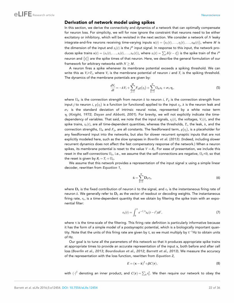
Derivation of network model using spikesIn this section, we derive the connectivity and dynamics of a network that can optimally compensate

for neuron loss. For simplicity, we will for now ignore the constraint that neurons need to be either

excitatory or inhibitory, which will be revisited in the next section. We consider a network of N leaky

integrate-and-fire neurons receiving time-varying inputs x tð Þ ¼ x1 tð Þ; . . .; xj tð Þ; . . .; xM tð Þ� �

, where M is

the dimension of the input and xj tð Þ is the jth input signal. In response to this input, the network pro-

duces spike trains s tð Þ ¼ s1 tð Þ; . . .; si tð Þ; . . .; sN tð Þð Þ, where si tð Þ ¼P

l d t � til� �

is the spike train of the ith

neuron and til�

are the spike times of that neuron. Here, we describe the general formulation of our

framework for arbitrary networks with N � M.

A neuron fires a spike whenever its membrane potential exceeds a spiking threshold. We can

write this as Vi>Ti, where Vi is the membrane potential of neuron i and Ti is the spiking threshold.

The dynamics of the membrane potentials are given by:

dVi

dt¼�lViþ

X

M

j¼1

Fijg xj� �

þX

N

k¼1

iksk þsVhi; (5)

where ik is the connection strength from neuron k to neuron i, Fij is the connection strength from

input j to neuron i, g xj� �

is a function (or functional) applied to the input xj, l is the neuron leak and

sV is the standard deviation of intrinsic neural noise, represented by a white noise term

hi (Knight, 1972; Dayan and Abbott, 2001). For brevity, we will not explicitly indicate the time-

dependency of variables. That said, we note that the input signals, xj tð Þ, the voltages, Vi tð Þ, and the

spike trains, sk tð Þ, are all time-dependent quantities, whereas the thresholds, Ti, the leak, l, and the

connection strengths, ik and Fij, are all constants. The feedforward term, g xj� �

, is a placeholder for

any feedforward input into the networks, but also for slower recurrent synaptic inputs that are not

explicitly modeled here, such as the slow synapses in Boerlin et al. (2013). (Indeed, including slower

recurrent dynamics does not affect the fast compensatory response of the network.) When a neuron

spikes, its membrane potential is reset to the value V ¼ Ri. For ease of presentation, we include this

reset in the self-connections ii, i.e., we assume that the self-connections are negative, ii<0, so that

the reset is given by Ri ¼ Tiþii.

We assume that this network provides a representation of the input signal x using a simple linear

decoder, rewritten from Equation 1,

x¼X

N

k¼1

Dkrk; (6)

where Dk is the fixed contribution of neuron k to the signal, and rk is the instantaneous firing rate of

neuron k. We generally refer to Dk as the vector of readout or decoding weights. The instantaneous

firing rate, rk, is a time-dependent quantity that we obtain by filtering the spike train with an expo-

nential filter:

rk tð Þ ¼Z

¥

0

e�t0=tsk t� t0ð Þdt0; (7)

where t is the time-scale of the filtering. This firing rate definition is particularly informative because

it has the form of a simple model of a postsynaptic potential, which is a biologically important quan-

tity. Note that the units of this firing rate are given by t, so we must multiply by t�1Hz to obtain units

of Hz.

Our goal is to tune all the parameters of this network so that it produces appropriate spike trains

at appropriate times to provide an accurate representation of the input x, both before and after cell

loss (Boerlin et al., 2013; Bourdoukan et al., 2012; Barrett et al., 2013). We measure the accuracy

of the representation with the loss function, rewritten from Equation 2,

E¼ x� xð Þ2þbC rð Þ; (8)

with �ð Þ2 denoting an inner product, and C rð Þ ¼P

k r2

k . We then require our network to obey the




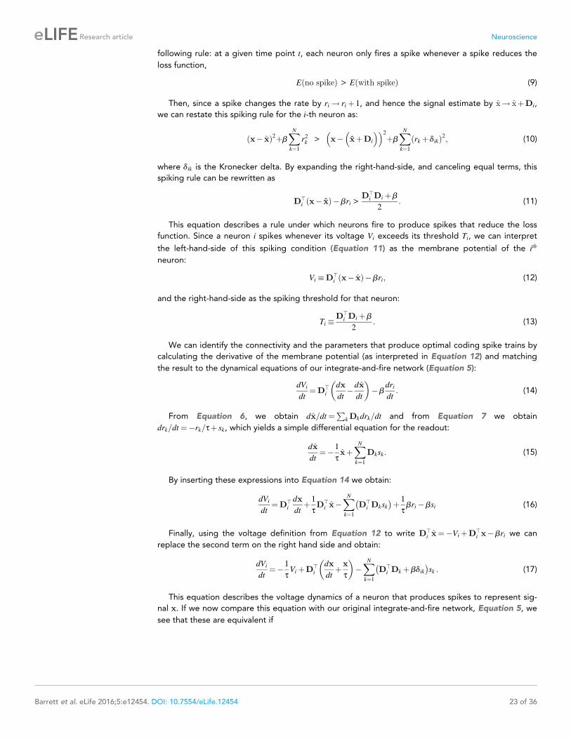
following rule: at a given time point t, each neuron only fires a spike whenever a spike reduces the

loss function,

Eðno spikeÞ > Eðwith spikeÞ (9)

Then, since a spike changes the rate by ri ! riþ 1, and hence the signal estimate by x! xþDi,

we can restate this spiking rule for the i-th neuron as:

x� xð Þ2þbX

N

k¼1

r2k > x� xþDi

� �� 2

þbX

N

k¼1

rk þ dikð Þ2; (10)

where dik is the Kronecker delta. By expanding the right-hand-side, and canceling equal terms, this

spiking rule can be rewritten as

D>i x� xð Þ�bri >

D>i Diþb

2: (11)

This equation describes a rule under which neurons fire to produce spikes that reduce the loss

function. Since a neuron i spikes whenever its voltage Vi exceeds its threshold Ti, we can interpret

the left-hand-side of this spiking condition (Equation 11) as the membrane potential of the ith

neuron:

Vi �D>i x� xð Þ�bri; (12)

and the right-hand-side as the spiking threshold for that neuron:

Ti �D

>i Di þb

2: (13)

We can identify the connectivity and the parameters that produce optimal coding spike trains by

calculating the derivative of the membrane potential (as interpreted in Equation 12) and matching

the result to the dynamical equations of our integrate-and-fire network (Equation 5):

dVi

dt¼D

>i

dx

dt� dx

dt

� �

�bdri

dt: (14)

From Equation 6, we obtain dx=dt¼P

kDkdrk=dt and from Equation 7 we obtain

drk=dt¼�rk=tþ sk, which yields a simple differential equation for the readout:

dx

dt¼�1

txþ

X

N

k¼1

Dksk: (15)

By inserting these expressions into Equation 14 we obtain:

dVi

dt¼D

>i

dx

dtþ 1

tD

>i x�

X

N

k¼1

D>i Dksk

� �

þ 1

tbri�bsi (16)

Finally, using the voltage definition from Equation 12 to write D>i x¼�Vi þD

>i x�bri we can

replace the second term on the right hand side and obtain:

dVi

dt¼�1

tViþD

>i

dx

dtþx

t

� �

�X

N

k¼1

D>i Dk þbdik

� �

sk : (17)

This equation describes the voltage dynamics of a neuron that produces spikes to represent sig-

nal x. If we now compare this equation with our original integrate-and-fire network, Equation 5, we

see that these are equivalent if




ik �� D>i Dk þbdik

� �

; (18)

Fij � ½Di�j ; (19)

gðxjÞ �dxj

dtþ xj

t; (20)

l� 1

t; (21)

Ti �D

>i Di þb

2: (22)

Here, the notation ½z�j refers to the j-th element of the vector z. A network of integrate-and-fire

neurons with these parameters and connection strengths can produce spike trains that represent the

signal x to a high degree of accuracy. Elements of this calculation have been produced before

(Boerlin et al., 2013), but are reproduced here for the sake of completeness. Also, it has been

shown that this connectivity can be learned using simple spike timing-dependent plasticity rules (W.

Brendel, R. Bourdoukan, P. Vertechi, et al, unpublished observations; Bourdoukan et al. (2012)), so

extensive fine-tuning is not required to obtain these spiking networks. We note that the input into

the network consists of a combination of the original signal, xj, and its derivative, dxj=dt. This can be

interpreted in several ways. First, we can think of the original signal, xjðtÞ, as a filtered version of the

actual input, so that dxj=dt¼�lxjþ cjðtÞ, where cjðtÞ is the actual input (and note that

cj ¼ lxjþ dxj=dt). Second, we can think of this as a biophysical computation, in the sense that the neu-

ron receives two types of input, the original signal input, xjðtÞ, and its derivative, dxj=dt. The latter

could be computed through a simple circuit that combines direct excitatory signal inputs with

delayed inhibitory signal inputs (e.g. through feedforward inhibition).

Our derivation of network dynamics directly from our loss function allows us to interpret the prop-

erties of this network in terms of neural function. Each spike can be interpreted as a greedy error

reduction mechanism—it moves x closer to the signal x. This error reduction is communicated back

to the network through recurrent connectivity, thereby reducing the membrane potential of the

other neurons. The membrane potential, in turn, can be interpreted as a representation error—it is

determined by a linear projection of x� x onto the neuron’s decoding weights, Di (Equation 12).

Following this interpretation, whenever the error becomes too big, the voltage becomes too big

and it reaches threshold. This produces a spike, which reduces the error, and so on.

We can also understand these network dynamics in terms of attractor dynamics. This network

implements a point attractor—firing rates evolve towards a stable fixed point in N-dimensional firing

rate space. The location of this point attractor depends on neural input and network connectivity.

When a neuron dies, the point attractor is projected into a subspace given by rk ¼ 0, where neuron k

is the neuron that has died.

Note that in this derivation, we used a quadratic cost. This cost increases the value of the spiking

threshold (Equation 13) and the spiking reset (Equation 18). We can also derive network parame-

ters for alternative cost term choices. For example, if we use a linear cost, we simply need to drop

the second term (bdik) in Equation 18, while keeping all other parameters the same. In other words,

we can implement a quadratic cost by increasing the spiking threshold and the spiking reset, and we

can implement a linear cost by increasing the spiking threshold without increasing the spiking reset.

In this way, the spiking threshold, and the reset determine the cost function. It is conceivable that

these variables may be learned, just as network connectivity may be learned. Alternatively, these val-

ues may be predetermined for various brain areas, depending on the computational target of each

brain area.

Derivation of network model with separate excitatory and inhibitorypopulationsWhen these ideas are applied to large and heterogeneous networks, we run into one problem con-

cerning their biological interpretation. Individual neurons in these networks can sometimes target

postsynaptic neurons with both excitatory and inhibitory synapses, so that they violate Dale’s law.

To avoid this problem, we consider a network that consists of separate pools of excitatory and inhib-

itory neurons. The external signals feed only into the excitatory population, and the inhibitory popu-

lation remains purely local. This scenario is captured by the equations,




dVEi

dt¼�lVE

i þX

M

j¼1

FijgðxjÞþX

NE

k¼1

EEik sEk �

X

NI

k¼1

EIik s

Ik �RE

i sEi þsVhi ; (23)

dV Ii

dt¼�lV I

i þX

NE

k¼1

IEik s

Ek �

X

NI

k¼1

IIiks

Ik �RI

i sIi þsVhi : (24)

The four connectivity matrices, EEik , EI

ik , IEik ,

IIik are all assumed to have only positive entries,

which enforces Dale’s law in this network. The neuron’s self-resets are now explicitly captured in the

terms REi s

Ei and RI

i sIi , and are no longer part of the connectivity matrices themselves. We will now

show how to design the four connectivity matrices such that the resulting network becomes function-

ally equivalent to the networks in the previous section. To do so, we apply the basic ideas outlined

in Boerlin et al. (2013), and simplified due to W. Brendel, R. Bourdoukan, P. Vertechi, and the

authors (personal communication).

We start with the network in the previous section, as described in Equation 5, and split its (non-

Dalian) recurrent connectivity matrix, ik, into self-resets, excitatory connections, and inhibitory con-

nections. The self-resets are simply the diagonal entries of �ik, see Equation 18,

Ri ¼D>i Diþb ; (25)

where the choice of signs is dictated by the sign conventions in Equation 23 and Equation 24. The

excitatory connections are the positive entries of ik, for which we define

EEik ¼ ½�D

>i Dk �bdik�þ ; (26)

where the notation ½x�þ denotes a threshold-linear function, so that ½x�þ ¼ x if x>0 and ½x�þ ¼ 0 other-

wise. The inhibitory connections are the negative, off-diagonal entries of ik, for which we write

Wik ¼ ½D>i Dk þbdik�þ � dikRk : (27)

With these three definitions, we can re-express the recurrent connectivity as

ik ¼EEik �Wik � dikRk.

Using this split of the non-Dalian connectivity matrix, we can trivially rewrite Equation 5 as an

equation for an excitatory population,

dVEi

dt¼�lVE

i þX

M

j¼1

FijgðxjÞþX

NE

k¼1

EEik sEk �

X

NE

k¼1

WiksEk �RE

i sEi þsVhi ; (28)

which is identical to Equation 23 above, except for the term with the inhibitory synapses, Wik, on

the right-hand-side. Here, the inhibitory synapses are multiplied with sEk rather than sIk, and their

number is identical to the number of excitatory synapses. Accordingly, this term violates Dale’s law,

and we need to replace it with a genuine input from the inhibitory population. Since this non-Dalian

term consists of a series of delta-functions, we can only replace it approximately, which will suffice

for our purposes. We simply require that the genuine inhibitory input approximates the non-Dalian

term on the level of the postsynaptic potentials, i.e., the level of filtered spike trains,

X

NE

k¼1

WikrEk »

X

NI

k¼1

EIik r

Ik : (29)

Here the left-hand-side is the given non-Dalian input, and the right-hand-side is the genuine

inhibitory input, which we are free to manipulate and design.

The solution to the remaining design question is simple. In the last section, we showed how to

design arbitrary spiking networks such that they track a given set of signals. Following these recipes,

we assume that the inhibitory population output optimally tracks the (filtered) spike trains of the

excitatory population. More specifically, we assume that we can reconstruct the instantaneous firing

rates of the excitatory neurons, rEi , by applying a linear readout to the instantaneous firing rates of

the inhibitory neurons, rIj , so that




rE ¼

X

NI

j¼1

DIj r

Ij : (30)

Note that all entries of DIj , the inhibitory decoding weights, must be positive. If the estimate of

the excitatory firing rates closely tracks the real firing rates, then we can fulfil Equation 29.

To obtain this relation, we will assume that the inhibitory population minimizes its own loss

function,

EI ¼ ðrE � rEÞ2 þbICðrIÞ : (31)

where the first term is the error incurred in reconstructing the excitatory firing rates, and the second

term is a cost associated with the firing of the inhibitory neurons. Apart from the replacement of the

old input signal, x, by the new ‘input signal’, rE, this is exactly the same loss function as in Equa-

tion 8. An important difference is that here the number of input signals, which corresponds to the

number of excitatory neurons, may be larger than the number of output spike trains, which corre-

sponds to the number of inhibitory neurons. Our spiking networks will in this case still minimize the

mean-square-error above, though the representation could be lossy. Since the effective dimensional-

ity explored by the instantaneous firing rates of the excitatory population is limited by the

dimensionality of the input signal space, however, these losses are generally small for our purposes.

Given the above loss function, we can redo all derivations from the previous section, to obtain

the connections, thresholds, and resets for the inhibitory population. Defining the short-hand

HIik ¼ ðDI

i Þ>DIk þbIdik ; (32)

we find that

IIik �HI

ik �RIkdik ; (33)

IEik � ½DI

i �k ; (34)

Tk �HI

kk

2; (35)

RIk �HI

kk : (36)

Here the first equation is equivalent to Equation 18, except for the different sign convention (IIik

enters negatively in Equation 24), and for the subtraction of the self-reset term, which is not part of

the recurrent connectivity. The second equation is equivalent to Equation 19. The third equation is

equivalent to Equation 22, and the fourth equation is the self-reset term, containing the diagonal

elements of Equation 18. Note that, due to the positivity of the inhibitory decoding weights, the

two connectivity matrices have only positive entries, as presupposed above in Equation 24. Conse-

quently, the inhibitory subnetwork obeys Dale’s law.

In a last step, we replace the excitatory spike trains in Equation 28 with their inhibitory approxi-

mation. Specifically, we rewrite Equation 29 as

X

NE

k¼1

WikrEk »

X

NE

k¼1

Wik rEk (37)

¼X

NE

j¼1

X

NI

k¼1

WijDIjkr

Ik (38)

�X

NI

k¼1

EIik r

Ik ; (39)

where we used Equation 30 in the approximation step. This approximation generally works very

well for larger networks; in smaller networks, finite size effects come into play.

Finally, when we take into account the results from the previous section, write DEi for the excit-

atory decoder weight of the i-th neuron, and introduce the short-hand

HEik ¼ ðDE

i Þ>DEk þbEdik ; (40)




then we find that the excitatory subnetwork has the connections, thresholds, and resets (compare

Equation 25–Equation 27),

Fij ¼ ½DEi �j ; (41)

EEik ¼ �HE

ik

� �

þ ; (42)

EIik ¼

X

NE

j¼1

�

HEij

h i

þ�dijR

Ej

�

DIjk ; (43)

TEk �HE

kk

2; (44)

REk ¼HE

kk : (45)

Importantly, the EI network therefore consists of two populations, one excitatory, one inhibitory,

both of which minimize a loss function. As a consequence, the excitatory subnetwork will compen-

sate optimally as long as the inhibitory subnetwork remains fully functional. In this limit, the excit-

atory subnetwork is essentially identical to the networks discussed in the previous section. The

inhibitory subnetwork will also compensate optimally until its recovery boundary is reached. In the

following, we will focus on one subnetwork (and one loss function again). For notational simplicity,

we will leave out the superscript references ‘E’.

Tuning curves and quadratic programmingFor constant input signals, the instantaneous firing rates of the neurons will fluctuate around some

mean value. Our goal is to determine this mean value. We will start with the most general case, and

rewrite the instantaneous firing rates as riðtÞ ¼ �ri þ hiðt;�riÞ, were hiðt;�riÞ is a zero-mean ’noise’ term

that captures the fluctuations of the instantaneous firing rates around its mean value. Note that

these fluctuations may depend on the neuron’s mean rate. In turn, neglecting the costs for a

moment, we can average the objective function, Equation 8, over time to obtain

hEit ¼D

�

x�X

i

DiriðtÞ�2E

t(46)

¼ ðx�X

i

Di�riÞ2 þX

ij

D>i Djhhið�riÞhjð�rjÞit: (47)

For larger networks, we can assume that the spike trains of neurons are only weakly correlated,

so that hhið�riÞhjð�rjÞit ¼Varðhið�riÞÞdij. Here, Varðhið�riÞÞ is the variance of the noise term. We obtain

hEit ¼ ðx�X

i

Di�riÞ2 þX

i

kDik2Varðhið�riÞÞ: (48)

We furthermore notice that the spike train statistics are often Poisson (Boerlin et al., 2013), in

which case we can make the replacement Varðhið�riÞÞ ¼ �ri. The loss function then becomes a qua-

dratic function of the mean firing rate, which needs to be minimized under a positivity constraint on

the mean firing rate. This type of problem is known as ‘quadratic programming’ in the literature. In

this study, we focused on networks for which the contributions of the firing rate fluctuations can be

neglected, which is generally the case for sufficiently small readout weights and membrane voltage

noise (see Figure 4—figure supplement 3). In this case, we obtain the loss function used in

Equation 3,

hEit ¼ ðx�X

i

Di�riÞ2 þbCð�rÞ (49)

with the cost term included again.

In general, quadratic programming is mathematically intractable, so the objective function must

be minimized numerically. However, in networks with a small number of neurons, we can solve the

problem analytically and gain some insight into the nature of quadratic programming. Here, we do

this for the two neuron example (Figure 4A).

In this example, we assumed that the first neuron contributes with D1 ¼ ðw; cÞ to the readout, and

the second neuron with D2 ¼ ð�w; cÞ. Accordingly, the firing rates �r1 and �r2 are given by the solution

to the following equation:




�r1;�r2ð Þ ¼ arg min�r1�0;�r2�0

x�ðw�r1 �w�r2Þð Þ2þðrB�ðc�r1 þ c�r2ÞÞ2 þbð�r21þ�r2

2Þ

h i

; (50)

where x is the variable signal, and rB is the fixed background signal. The positivity constraint parti-

tions the solution of this equation into three regions, determined by the value of x: region R1 where

�r1 ¼ 0 and �r2 � 0, region R2 where �r1 � 0 and �r2 � 0, and region R3 where �r2 ¼ 0 and �r1 � 0 (Fig-

ure 4—figure supplement 1A). In region 2, we can then easily solve Equation 50 by setting the

derivative of our loss function to zero. This gives �r¼ ðw>wþ c

>cþb1Þ�1ðwxþ crBÞ where

w¼ ðw;�wÞ, c¼ ðc;cÞ, and 1 is the identity matrix. Looking at this equation, we see that �r1 ¼ 0 when

x¼�crB=w and �r2 ¼ 0 when x¼ crB=w. Therefore, the firing rate solution for region two is valid when

�crB=w� x� crB=w. For x� crB=w, we have �r2 ¼ 0 because of the positivity constraint in Equation 50.

This is region 3. We can calculate �r1 by setting �r2 ¼ 0 and then minimizing the loss function. This

gives �r1 ¼ ðw2 þ c2þbÞ�1ðwxþ crBÞ. Similarly, for x��crb=w we have �r1 ¼ 0 because of the positivity

constraint. This is region one and we obtain �r2 ¼ ðw2 þ c2 þbÞ�1ð�wxþ crBÞ. The firing rates within

each region are given by a simple linear projection of x0 ¼ ðx; rBÞ, although the size and direction of

this projection is different in each region. As such, the solution to this quadratic programming prob-

lem is a piece-wise linear function of x.

In networks with larger numbers of neurons, the solution will still be a piece-wise linear function

of x, although there will be more regions and the firing rate solutions are more complicated because

more neurons are simultaneously active. In contrast, the transformation from firing rates to x0 is very

simple (Equation 6). It is given by a simple linear transformation, and is region independent (Fig-

ure 4—figure supplement 1B).

Readout weights and cost terms: 1-d and 2-d exampleThere are a number of free parameters in our model, such as the cost terms and the readout

weights. The choice of these values determine the precise shape of tuning curves. In general, how-

ever, the precise values of these terms have little influence on the coding capability of our system,

once certain properties have been satisfied, which we will outline here.

The cost term that we used for the examples in Figures 1–6 is a quadratic cost, CðrÞ ¼ P

k r2

k .

This cost term encourages the system to find a solution in which all neurons share in the signal repre-

sentation. (Here, and in the following, we will no longer distinguish ri, the instantaneous firing rate

used in the spiking network, and �ri, the mean firing rates used in quadratic programming. The

appropriate notation will be determined by the context.) The cost term for Figures 7–9, the V1

model, is a linear cost, CðrÞ ¼ P

k rk. This cost term limits the overall number of spikes, and generally

encourages sparse solutions, in which most neurons contribute very little to the signal representa-

tion. Regardless of this choice, our general predictions about optimal compensation are qualitatively

similar, as long as the cost term does not dominate the loss function.

The other important parameters that we must choose are the decoding or readout weights. In

Figure 2, the decoding weights of the excitatory population were drawn from a Gaussian distribu-

tion with mean �E ¼ 2, and standard deviation sE ¼ 0:2. For the inhibitory population, we used a

mean �I ¼ 0:3 and a standard deviation sI ¼ 0:03. For the networks in Figures 3–6, we have used

regularly spaced decoding weights, with the addition of some random noise. The parameter values

that we used are plotted in Figure 3D, Figure 4A–C, left column, and Figure 5A,E,I.

All of our quadratic programming and optimal compensation predictions for tuning curve shapes

still hold for alternative choices of readout weights, once the following properties are satisfied. First,

it is important that the readout vectors span the space of the signal that we want our network to

represent. Otherwise, the system will not be able to represent signals along certain directions, or

compensate for neuron loss. Second, it is important to set the scale of the readout, so that the cost

does not dominate. There is a natural scaling that we can use to avoid such problems. We require

the size of firing rates and the readout to be independent of network size. From

xj ¼PN

k Djkrk ~Oð1Þ, it follows that Djk ~Oð1=NÞ. As a consequence, the off-diagonal elements of the

recurrent connectivity are small ik ~Oð1=N2Þ, for i 6¼ k (Equation 18), and if we assume that the

diagonal elements are on the same order of magnitude, then b ~Oð1=N2Þ. This scaling provides a

principled basis for parameter choices in our model.




We may also want to scale our decoder weights without changing the shape of our tuning curve

prediction (Figure 4—figure supplement 3B). To do this, the cost parameter b and the membrane

potential leak l must also be scaled together. Specifically, if the readout weights are given by

a� Djk

�

, where a is a scaling parameter that characterizes the size of the decoder weights and

Djk

�

are fixed decoder weights, then the spiking cost parameter must be set to a2 � b and the

membrane potential leak must be set to a� l. We can see that this preserves the shape of tuning

curves by looking at the resulting structure of our loss function (Equation 2):

EðrÞ ¼ ðx�ðaDÞ � rÞ2 þa2bP

N

i¼1

ri2 : (51)

As before, the minimum of this loss function gives firing rates in units of the inverse membrane

potential leak ðalÞ. Therefore, we must divide r by ðalÞ to obtain firing rates in units of Hz. Our loss

function then becomes:

Eðr=ðalÞÞ ¼ ðx�ðaDÞ � r=ðalÞÞ2 þa2bX

i

ri=ðalÞð Þ2 (52)

¼ ðx�D � r=lÞ2 þbX

i

ri=lð Þ2 : (53)

This loss function is independent of a, and so, using this scaling the optimal tuning curves will

have the same shape for all values of a.

Readout weights and cost terms: V1 exampleThere are many possible choices of decoder weights Dif g that provide a faithful representation of a

signal. In positive sparse coding, we choose the decoder weights that provide the most efficient sig-

nal representation, for a sparse cost term (CðrÞ ¼ P

k rk), under the constraint that firing rates must

be positive. Here, we describe how we calculate these positive sparse coding weights, which we will

use in several of our figures (Figures 7–9 and Figure 9—figure supplement 1–2).

We use the signal vector x ¼ ðx1; . . . ; xj; . . . ; xMÞ to denote an image patch, where each element xjrepresents a pixel from the image patch (Olshausen and Field, 1996). We quantify the efficiency of

a sparse representation using the following loss function:

E¼ ðx� xÞ2D E

þbX

i

ri

* +

; (54)

where :::h i denotes an average across image patches. This is simply Equation 2 with a sparse cost

term, averaged over image patches. The first term in this loss function is the image representation

error. The second term quantifies the sparsity of the representation. The decoding filters that mini-

mize this loss function will be the positive sparse coding filters for natural images.

We assume that the decoding filters are optimized to represent natural images, such as forest

scenes, flowers, sky, water and other images from nature. Natural images are chosen because they

are representative of the images that surround animals throughout evolution. We randomly select

2000 image patches of size 12� 12 from eight natural images taken from Van Hateren’s Natural

Image Database (van Hateren and van der Schaaf, 1998). These images are preprocessed by

removing low-order statistics, so that our sparse coding algorithm can more easily learn the higher-

order statistical structure of natural images. First of all, images are centered so as to remove first

order statistics:

x! x� xh i: (55)

Next, images are whitened, so as to remove second-order statistics:

x!M�1=2

x ; (56)

where M¼ xxTh i is a decorrelating matrix.




We calculate sparse coding filters by minimizing the loss function (Equation 54) using a two step

procedure. First, for each image patch in a subset of 50 image patches, we calculate the firing rates

that minimize the loss function under the constraint that firing rates must be positive:

r¼ arg minri�0 8i

E : (57)

The positivity constraint reduces the representational power of the neural population, so, to coun-

teract this, we use a large population containing twice as many neurons as signal dimensions, N ¼2M and we initialize our decoder matrix to Djk ¼ dj;k � dj;kþM to ensure that our neural population can

easily span the signal space throughout the sparse coding calculation.

Next, we update our decoding vectors by stochastic gradient descent on the loss function, using

the optimal firing rates calculated in the previous step:

Di !Di� �dE

dDi

¼Diþ �2 ðx� xÞrih i : (58)

Decoding weights are normalized for each neuron, so that they do not become arbitrarily large.

This calculation is similar to sparse coding calculations performed before (Olshausen and Field,

1996), except that we enforce the additional requirement that firing rates must be positive. This

constraint was used before for sparse non-negative matrix factorization (Hoyer, 2003, 2004). How-

ever, this method requires an additional constraint that decoding weights be strictly positive, so that

the non-negative matrix factorization method can be applied. This additional constraint will reduce

the efficiency of the representation, because it precludes solutions that may be more efficient, but

violate the additional constraint.

To compare the properties of optimal compensation in this positive sparse coding model to

experiment, we calculate the direction tuning of neurons in our model using a protocol similar to

that used in the experimental work (Crook and Eysel, 1992). Specifically, we drive our model using

a directed, edge-like stimulus. These stimuli are Gabor filters, with a profile similar to the sparse cod-

ing filters. We calculate the firing rate response of each neuron using Equation 57 for 16 different

stimulus directions. For each direction, the Gabor filter is positioned at regularly spaced locations

along a line perpendicular to the Gabor filter orientation and the maximum firing rate of each neu-

ron along this line is taken as the firing rate response of that neuron at that direction. These firing

rate responses form the direction tuning curves that we can compare to experimental recordings.

The impact of neuron lossWe investigate the impact of neuron loss in our spiking model by simulating the network both

before and after neuron loss (Figure 2 and Figure 3). Specifically, we use the Euler method to iter-

ate the dynamics described by Equation 17 or Equation 23, Equation 24, and we measure the

readout x, the spike trains s, and the membrane potentials V. We simulate the loss of a neuron by

setting all the connections to and from that neuron to zero. This is equivalent to silencing a neuron.

We continue to measure the network activity and the readout after neuron loss.

We also calculate the impact of neuron loss on tuning curves with and without optimal compensa-

tion (Figure 5). To calculate tuning curves without compensation we solve Equation 3 in the intact

state. We then constrain the firing rates of neurons selected for loss to zero and calculate the impact

of this on our signal representation. To calculate the impact of neuron loss with optimal compensa-

tion, we solve Equation 4.

The integrate-and-fire model that we have described can produce spikes at arbitrarily large firing

rates. This can be a problem, especially when neurons die and the remaining neurons compensate

with extremely high, unrealistic firing rates. To avoid this, we can include a form of adaptation in our

spiking model. Specifically, we can extend our spiking rule so that a neuron i will only spike if its fir-

ing rate fi is lower than a maximum fmax. Here, the firing rate f is given by the following differential

equation:

df

dt¼�f=tAþ s ; (59)

and tA is the time scale of adaptation. This time scale is much slower than the time scale of




the spiking dynamics t. We use this extended neural model to calculate the recovery boundary in

Figure 3J,K, where we kill neurons in random order.

In turn, we can compute the firing rates and recovery boundary of this extended integrate-and-

fire model using quadratic programming (data not shown). Specifically, the firing rates of this net-

work are given by the solution of the following optimization problem:

rðxÞ ¼ argminR

EðxÞ ; (60)

where R denotes the set of constraints that the firing rates must satisfy:

R¼ rmax � ri � 08 i; rj ¼ 08j 2 X�

(61)

and where X is the set of all dead (or silenced) neurons.

To study the effects of redundancy (or overcompleteness) in the V1 model (Figure 9—figure sup-

plement 2A), we define an over-completeness factor, K, given by K ¼ N=M, where N is the number

of neurons in the representation and M is the signal dimension. In the sparse coding calculation

above, we had K ¼ 2. To increase the redundancy or overcompleteness of the representation, we

generated a new set of readout vectors by two methods. In method one, we randomly drew N ¼KM decoding vectors D

ðKÞi from the V1 model and then added multiplicative noise, in order to avoid

parallel readout weights. Specifically, the new readout vectors DðKÞi were obtained from the old

readout vectors, Dð2Þi , using D

ðKÞiþa ¼ D

ð2Þi � ð1þ jiþaÞ=ðK=2Þ, where i 2 ½1; . . . ; 2M�, �ij ~Nð0; 0:1Þ, a ¼

2Mm and m 2 ½0; . . . ;K=2� 1�. In method two, we also randomly drew decoding vectors from the V1

model, but then shifted the corresponding 12� 12 image patch randomly in space. Both methods

yielded similar results. We used these methods to calculate readout weights for over-complete rep-

resentations because the sparse coding calculation becomes computationally prohibitive for large

values of M.

Tight balance of excitation and inhibitionIn simulations of our spiking model, we see that optimal coding generally coincides with a balance

of excitatory and inhibitory currents into each neuron (Figure 2G and Figure 3H,I). To characterize

this balance, we define three currents for each excitatory neuron. First, we define the excitation Ei as

the total input current received through excitatory synapses. Second, we define the inhibition Ii as

the total input current received through inhibitory synapses. Third, we define the reset current �Ri as

the total current caused by a neuron’s self-reset after an action potential. Since our idealized neuron

model uses delta-functions to capture the synaptic currents evoked by single spikes, we smooth the

delta-functions in order to obtain more realistic synaptic currents. For simplicity, we use the same fil-

ter as in the computation of the instantaneous firing rates, although other filters could be used as

well. In the EI network, Equation 23 and Equation 24, the three currents into the i-th excitatory neu-

ron are then given by

Ei ¼X

N

k¼1

EEik rEk þ

X

M

j¼1

FEij xj ; (62)

Ii ¼X

N

k¼1

EIik r

Ik þ

X

M

j¼1

FIijxj ; (63)

�Ri ¼ REi r

Ei ; (64)

where FEij � Fij if Fijxj>0 (and FE

ij � 0 otherwise), and FIij � Fij if Fijxj<0 (and FI

ij � 0 otherwise). When

the inhibitory subpopulation is not explicitly simulated, we simply set EEik rEk �ikrk unless ik<0 and

EIik r

Ik �ikrk unless ik>0.

Using the above definitions of currents, we can integrate Equation 23 to re-express the voltage

of an excitatory neuron as VEi ¼ Ei � Ii � �Ri. This voltage is trivially bounded from above by a neu-

ron’s threshold, VEi <Ti. Due to the design properties of the network, the voltage is also bounded

from below: since the voltage reflects a representation error, neurons with decoding vectors oppo-

site to those of neuron i will keep negative errors in check. If we neglect cost terms, we obtain




VEi >R

Ei . (Otherwise the bound is lower). Re-expressed for the EI ratio, we obtain the following

bounds

1þ�Ri �RE

i

Ii<

Ei

Ii< 1þ

�RiþTi

Ii: (65)

The EI ratio will therefore approach one (perfect balance) if the inhibitory synaptic currents are

much larger than the self-reset currents and voltage thresholds, or, if excitatory currents are can-

celled by inhibitory currents rather than by a neuron’s spikes and subsequent self-resets.

The network does not reach this balanced regime under two conditions. First, if a network has a

small redundancy, i.e., the number of neurons, N, is not much larger than the number of input sig-

nals, M, then each neuron carries a large load of the representation, and the reset currents become

similar in magnitude to the synaptic currents. This is the case for the cricket cercal system, for

instance, for which N ¼ 4 and M ¼ 2. Second, if a system approaches the recovery boundary, the

representational burden of some neurons also increases a lot, leading to a similar effect. This is the

case for the green neuron in Figure 3I, even after the first k.o, and leads to a more regular firing pat-

tern. In other words, neurons that compensate for neuron loss can sometimes experience excessive

excitatory currents, even if the compensation is successful.

To capture the mechanistic difference between compensation and recovery boundary more

clearly, we therefore also defined the ratio of positive to negative currents, Ei=ðIi þ �RiÞ (Figure 3H).

This ratio is bounded by

1� REi

Iiþ �Ri

<Ei

Ii þ �Ri

<1þ Ti

Ii þ �Ri

: (66)

and remains close to one as long as there are sufficiently large negative currents, or, if excitatory cur-

rents are cancelled by either recurrent inhibition or by spiking. As long as the network is fully func-

tional, the latter will always be the case. Once the recovery boundary is hit, however, the lower

bound on the voltages of some neurons disappears, and so will the lower bound on the above ratio

of positive to negative currents (as well as the EI ratio), which is the effect we observe in Figure 3HI.

Traditionally, balance is often understood in the limit of very large networks (van Vreeswijk and

Sompolinsky, 1996, 1998), and these classical scaling arguments can also be applied to our net-

works (Boerlin et al., 2013). Neglecting Dale’s law once more for simplicity, we can increase the net-

work size, while keeping the relative size and number of the input signals and the neuron’s firing

rates constant. Since xj ¼P

k Djkrk ~Oð1Þ and rk ~Oð1Þ, we find that Djk ~Oð1=NÞ and b ~Oð1=N2Þ. Asa consequence of Equation 18 and Equation 13, we observe that both the recurrent connection

strengths and the spiking thresholds are small, so that ik ~Oð1=N2Þ and Ti ~Oð1=N2Þ. Now, because

recurrent input is summed across the entire population of N neurons, we find that

Vi ~OðN=N2Þ~Oð1=NÞ, and similar observations hold for Ii, Ei, and �Ri. Hence, these currents are N

times larger than the spiking threshold, Ti, or the reset, Ri. The EI ratio in Equation 65 then

approaches one, and excitatory and inhibitory currents cancel precisely. We note that this balance of

excitation and inhibition is much tighter than in balanced networks with random connectivity

(van Vreeswijk and Sompolinsky, 1996, 1998). In randomly connected networks the balance

between excitation and inhibition is of order Oð1=ffiffiffiffi

Np

Þ (van Vreeswijk and Sompolinsky, 1998),

whereas here these fluctuations are Oð1=NÞ. We note that these observations only hold when the

number of input signals, M, is kept constant; if that number grows with N, then the scaling is differ-

ent. The conceptual differences between loose and tight balance were recently highlighted in a

review (Deneve and Machens, 2016).

Optimal compensation proofThe spiking network that we use is capable of rapidly implementing optimal compensation, without

requiring any synaptic plasticity mechanisms. We can prove this by showing that an optimal network

of N � 1 neurons is equivalent to an optimal network of N neurons after the loss of one neuron. For

the EI network, the argument applies separately to the excitatory and inhibitory subnetworks.

For the sake of argument, we suppose that the N th neuron dies. At a mechanistic level, the loss of

this neuron is equivalent to cutting all the connections to and from the dead neuron and from the




dead neuron to the readout x. Therefore, a network where the N th neuron has died is equivalent to

a network with N � 1 neurons with readout matrix D�ij ¼ Dij 8j 2 ½1;N � 1� and 8i 2 ½1;M�, with feed-

forward connectivity F�ij ¼ Fij 8i 2 ½1;N � 1� and 8j 2 ½1;M�, with recurrent connectivity �

ik ¼ik 8i; k 2 ½1;N � 1� and with spiking thresholds T�

i ¼ �ii=28i 2 ½1;N � 1�.Now, we compare this damaged network to an optimal network consisting of N � 1 neurons. To

make a fair comparison, we assume that this network has the same readout matrix D0 � D

� as the

reduced damaged network. Then, the recurrent connectivity for this network is given by 0 ¼

�,

the feedforward connectivity is given by F0 � F

� and the spiking thresholds are given by T0 � T

�.This configuration is equivalent to the reduced damaged network. Therefore, a spiking neural net-

work whose neurons are individually tuned to represent a signal optimally before cell loss will per-

form optimal compensation and provide an optimal signal representation after cell loss.

AcknowledgementsWe thank Tony Movshon, Pedro Goncalves, and Wieland Brendel for stimulating discussions and

Alfonso Renart, Claudia Feierstein, Joe Paton, and Michael Orger for helpful comments on the man-

uscript. S.D. acknowledges the James McDonnell Foundation Award and EU grants BACS FP6-IST-

027140, BIND MECT-CT-20095–024831, and ERC FP7-PREDSPIKE. C.K.M. acknowledges an Emmy-

Noether grant of the Deutsche Forschungsgemeinschaft and a Chaire d’excellence of the Agence

National de la Recherche.

Additional information

Funding

Funder Grant reference number Author

Deutsche Forschungsge-meinschaft

Emmy-Noether Christian K Machens

Agence Nationale de Re-cherche

Chaire d’Excellence Christian K Machens

James S. McDonnell Founda-tion

Sophie Deneve

European Research Council ERC FP7-PREDSPIKE Sophie Deneve

European Research Council BIND MECT-CT-20095-024831

Sophie Deneve

European Research Council BACS 796 FP6-IST-027140 Sophie Deneve

The funders had no role in study design, data collection and interpretation, or the decision tosubmit the work for publication.

Author contributions

DGTB, CKM, Designed the study, Performed the analysis, Wrote the manuscript; SD, Designed the

study

Author ORCIDs

Christian K Machens, http://orcid.org/0000-0003-1717-1562

ReferencesAbbott LF. 2008. Theoretical neuroscience rising. Neuron 60:489–495. doi: 10.1016/j.neuron.2008.10.019,PMID: 18995824

Aksay E, Baker R, Seung HS, Tank DW. 2000. Anatomy and discharge properties of pre-motor neurons in thegoldfish medulla that have eye-position signals during fixations. Journal of Neurophysiology 84:1035–1049.PMID: 10938326

Aksay E, Olasagasti I, Mensh BD, Baker R, Goldman MS, Tank DW. 2007. Functional dissection of circuitry in aneural integrator. Nature Neuroscience 10:494–504. doi: 10.1038/nn1877

Amit DJ, Brunel N. 1997. Model of global spontaneous activity and local structured activity during delay periodsin the cerebral cortex. Cerebral Cortex 7:237–252. doi: 10.1093/cercor/7.3.237, PMID: 9143444



http://orcid.org/0000-0003-1717-1562

http://dx.doi.org/10.1016/j.neuron.2008.10.019

http://www.ncbi.nlm.nih.gov/pubmed/18995824


http://dx.doi.org/10.1038/nn1877

http://dx.doi.org/10.1093/cercor/7.3.237



Atick JJ. 1992. Could information theory provide an ecological theory of sensory processing? Network:Computation in Neural Systems 3:213–251. doi: 10.1088/0954-898X_3_2_009

Barlow H. 1961. Possible principles underlying the transformation of sensory messages. In: Rosenblith W. A (Ed).Sensory Communication. p. 217–234.

Barrett DGT, Deneve S, Machens CK. 2013. Firing rate predictions in optimal balanced networks. Advances inNeural Information Processing Systems 26. p. 1538–1546.

Bell AJ, Sejnowski TJ. 1997. The "independent components" of natural scenes are edge filters. Vision Research37:3327–3338. doi: 10.1016/S0042-6989(97)00121-1, PMID: 9425547

Ben-Yishai R, Bar-Or RL, Sompolinsky H. 1995. Theory of orientation tuning in visual cortex. PNAS 92:3844–3848.doi: 10.1073/pnas.92.9.3844, PMID: 7731993

Boerlin M, Deneve S. 2011. Spike-based population coding and working memory. PLoS Computational Biology7:e1001080. doi: 10.1371/journal.pcbi.1001080, PMID: 21379319

Boerlin M, Machens CK, Deneve S. 2013. Predictive coding of dynamical variables in balanced spiking networks.PLoS Computational Biology 9:e1003258. doi: 10.1371/journal.pcbi.1003258, PMID: 24244113

Bourdoukan R, Barrett DGT, Machens CK, Deneve S. 2012. Learning optimal spike-based representations.Advances in Neural Information Processing 25. p. 2294–2302.

Braun DA, Aertsen A, Wolpert DM, Mehring C. 2009. Learning optimal adaptation strategies in unpredictablemotor tasks. Journal of Neuroscience 29:6472–6478. doi: 10.1523/JNEUROSCI.3075-08.2009, PMID: 19458218

Bredesen DE, Rao RV, Mehlen P. 2006. Cell death in the nervous system. Nature 443:796–802. doi: 10.1038/nature05293, PMID: 17051206

Bromfield EB. 2006. An introduction to epilepsy. American Epilepsy Society.Charles AS, Garrigues P, Rozell CJ. 2012. A common network architecture efficiently implements a variety ofSparsity-Based inference problems. Neural Computation 24:3317–3339. doi: 10.1162/NECO_a_00372

Crook JM, Eysel UT. 1992. GABA-induced inactivation of functionally characterized sites in cat visual cortex (area18): effects on orientation tuning. Journal of Neuroscience 12:1816–1825. PMID: 1578272

Crook JM, Kisvarday ZF, Eysel UT. 1996. GABA-induced inactivation of functionally characterized sites in catvisual cortex (area 18): effects on direction selectivity. Journal of Neurophysiology 75:2071–2088. PMID:8734604

Crook JM, Kisvarday ZF, Eysel UT. 1997. GABA-induced inactivation of functionally characterized sites in catstriate cortex: effects on orientation tuning and direction selectivity. Visual Neuroscience 14:141–158. doi: 10.1017/S095252380000883X, PMID: 9057276

Crook JM, Kisvarday ZF, Eysel UT. 1998. Evidence for a contribution of lateral inhibition to orientation tuningand direction selectivity in cat visual cortex: reversible inactivation of functionally characterized sites combinedwith neuroanatomical tracing techniques. European Journal of Neuroscience 10:2056–2075. doi: 10.1046/j.1460-9568.1998.00218.x, PMID: 9753093

Dayan P, Abbott L. 2001. Theoretical Neuroscience: Computational and Mathematical Modeling of NeuralSystems. Cambridge, Massachusetts: MIT Press.

Deneve S, Machens CK. 2016. Efficient codes and balanced networks. Nature Neuroscience 19:375–382. doi: 10.1038/nn.4243, PMID: 26906504

Druckmann S, Chklovskii DB. 2012. Neuronal circuits underlying persistent representations despite time varyingactivity. Current Biology 22:2095–2103. doi: 10.1016/j.cub.2012.08.058, PMID: 23084992

Fairhall AL, Lewen GD, Bialek W, de Ruyter Van Steveninck RR. 2001. Efficiency and ambiguity in an adaptiveneural code. Nature 412:787–792. doi: 10.1038/35090500, PMID: 11518957

Fenno L, Yizhar O, Deisseroth K. 2011. The development and application of optogenetics. Annual Review ofNeuroscience 34:389–412. doi: 10.1146/annurev-neuro-061010-113817, PMID: 21692661

Fuchs AF, Scudder CA, Kaneko CR. 1988. Discharge patterns and recruitment order of identified motoneuronsand internuclear neurons in the monkey abducens nucleus. Journal of Neurophysiology 60:1874–1895.PMID: 2466962

Goncalves PJ, Arrenberg AB, Hablitzel B, Baier H, Machens CK. 2014. Optogenetic perturbations reveal thedynamics of an oculomotor integrator. Frontiers in Neural Circuits 8:10. doi: 10.3389/fncir.2014.00010,PMID: 24616666

Greene G, Barrett DGT, Sen K, Houghton C. 2009. Sparse coding of birdsong and receptive field structure insongbirds. Network: Computation in Neural Systems 20:162–177. doi: 10.1080/09548980903108267, PMID: 19731147

Haas JS, Nowotny T, Abarbanel HD. 2006. Spike-timing-dependent plasticity of inhibitory synapses in theentorhinal cortex. Journal of Neurophysiology 96:3305–3313. doi: 10.1152/jn.00551.2006, PMID: 16928795

Hennequin G, Vogels TP, Gerstner W. 2014. Optimal control of transient dynamics in balanced networkssupports generation of complex movements. Neuron 82:1394–1406. doi: 10.1016/j.neuron.2014.04.045,PMID: 24945778

Hopfield JJ. 1984. Neurons with graded response have collective computational properties like those of two-state neurons. PNAS 81:3088–3092. doi: 10.1073/pnas.81.10.3088

Horn D, Levy N, Ruppin E. 1996. Neuronal-based synaptic compensation: a computational study in Alzheimer’sdisease. Neural Computation 8:1227–1243. doi: 10.1162/neco.1996.8.6.1227, PMID: 8768393

Hoyer P. 2004. Non-negative matrix factorization with sparseness constraints. The Journal of Machine LearningResearch 5:1457–1469.

Hoyer PO. 2003. Modeling receptive fields with non-negative sparse coding. Neurocomputing 52-54:547–552.doi: 10.1016/S0925-2312(02)00782-8



http://dx.doi.org/10.1088/0954-898X_3_2_009

http://dx.doi.org/10.1016/S0042-6989(97)00121-1


http://dx.doi.org/10.1073/pnas.92.9.3844


http://dx.doi.org/10.1371/journal.pcbi.1001080




http://dx.doi.org/10.1523/JNEUROSCI.3075-08.2009


http://dx.doi.org/10.1038/nature05293



http://dx.doi.org/10.1162/NECO_a_00372



http://dx.doi.org/10.1017/S095252380000883X

http://dx.doi.org/10.1017/S095252380000883X


http://dx.doi.org/10.1046/j.1460-9568.1998.00218.x

http://dx.doi.org/10.1046/j.1460-9568.1998.00218.x


http://dx.doi.org/10.1038/nn.4243



http://dx.doi.org/10.1016/j.cub.2012.08.058


http://dx.doi.org/10.1038/35090500


http://dx.doi.org/10.1146/annurev-neuro-061010-113817



http://dx.doi.org/10.3389/fncir.2014.00010


http://dx.doi.org/10.1080/09548980903108267



http://dx.doi.org/10.1152/jn.00551.2006




http://dx.doi.org/10.1073/pnas.81.10.3088

http://dx.doi.org/10.1162/neco.1996.8.6.1227


http://dx.doi.org/10.1016/S0925-2312(02)00782-8


Hu T, Genkin A, Chklovskii DB. 2012. A network of spiking neurons for computing sparse representations in anenergy-efficient way. Neural Computation 24:2852–2872. doi: 10.1162/NECO_a_00353, PMID: 22920853

Hubel DH, Wiesel TN. 1962. Receptive fields, binocular interaction and functional architecture in the cat’s visualcortex. The Journal of Physiology 160:106–154. doi: 10.1113/jphysiol.1962.sp006837, PMID: 14449617

Keck T, Mrsic-Flogel TD, Vaz Afonso M, Eysel UT, Bonhoeffer T, Hubener M. 2008. Massive restructuring ofneuronal circuits during functional reorganization of adult visual cortex. Nature Neuroscience 11:1162–1167.doi: 10.1038/nn.2181, PMID: 18758460

King PD, Zylberberg J, DeWeese MR. 2013. Inhibitory interneurons decorrelate excitatory cells to drive sparsecode formation in a spiking model of V1. Journal of Neuroscience 33:5475–5485. doi: 10.1523/JNEUROSCI.4188-12.2013, PMID: 23536063

Knight BW. 1972. Dynamics of encoding in a population of neurons. The Journal of General Physiology 59:734–766. doi: 10.1085/jgp.59.6.734

Kording KP, Tenenbaum JB, Shadmehr R. 2007. The dynamics of memory as a consequence of optimaladaptation to a changing body. Nature Neuroscience 10:779–786. doi: 10.1038/nn1901, PMID: 17496891

Leary MC, Saver JL. 2003. Annual incidence of first silent stroke in the united States: a preliminary estimate.Cerebrovascular Diseases 16:280–285. doi: 10.1159/000071128, PMID: 12865617

Lee DD, Seung HS. 1999. Learning the parts of objects by non-negative matrix factorization. Nature 401:788–791. doi: 10.1038/44565, PMID: 10548103

Li N, Daie K, Svoboda K, Druckmann S. 2016. Robust neuronal dynamics in premotor cortex during motorplanning. Nature 532:459–464. doi: 10.1038/nature17643, PMID: 27074502

Libersat F, Mizrahi A. 1996. In situ visualization and photoablation of individual neurons using a low cost fiberoptic based system. Journal of Neuroscience Methods 67:157–162. doi: 10.1016/0165-0270(96)00043-X,PMID: 8872881

Lim S, Goldman MS. 2013. Balanced cortical microcircuitry for maintaining information in working memory.Nature Neuroscience 16:1306–1314. doi: 10.1038/nn.3492, PMID: 23955560

Luz Y, Shamir M. 2012. Balancing feed-forward excitation and inhibition via hebbian inhibitory synaptic plasticity.PLoS Computational Biology 8:e1002334. doi: 10.1371/journal.pcbi.1002334, PMID: 22291583

Machens CK, Gollisch T, Kolesnikova O, Herz AV. 2005. Testing the efficiency of sensory coding with optimalstimulus ensembles. Neuron 47:447–456. doi: 10.1016/j.neuron.2005.06.015, PMID: 16055067

Mizrahi A, Libersat F. 1997. Independent coding of wind direction in cockroach giant interneurons. Journal ofNeurophysiology 78:2655–2661. PMID: 9356415

Montague PR, Dolan RJ, Friston KJ, Dayan P. 2012. Computational psychiatry. Trends in Cognitive Sciences 16:72–80. doi: 10.1016/j.tics.2011.11.018, PMID: 22177032

Morrison JH, Hof PR. 1997. Life and death of neurons in the aging brain. Science 278:412–419. doi: 10.1126/science.278.5337.412, PMID: 9334292

Olshausen BA, Field DJ. 1996. Emergence of simple-cell receptive field properties by learning a sparse code fornatural images. Nature 381:607–609. doi: 10.1038/381607a0, PMID: 8637596

Palop JJ, Chin J, Mucke L. 2006. A network dysfunction perspective on neurodegenerative diseases. Nature 443:768–773. doi: 10.1038/nature05289, PMID: 17051202

Pastor AM, Gonzalez-Forero D. 2003. Recruitment order of cat abducens motoneurons and internuclear neurons.Journal of Neurophysiology 90:2240–2252. doi: 10.1152/jn.00402.2003, PMID: 12801900

Renart A, de la Rocha J, Bartho P, Hollender L, Parga N, Reyes A, Harris KD. 2010. The asynchronous state incortical circuits. Science 327:587–590. doi: 10.1126/science.1179850

Rieke F, Warland D, Steveninck deRvan RR, Bialek W. 1997. Spikes - Exploring the Neural Code. Cambridge,Massachusetts: MIT Press.

Rozell CJ, Johnson DH, Baraniuk RG, Olshausen BA. 2008. Sparse coding via thresholding and local competitionin neural circuits. Neural Computation 20:2526–2563. doi: 10.1162/neco.2008.03-07-486, PMID: 18439138

Salinas E. 2006. How behavioral constraints may determine optimal sensory representations. PLoS Biology 4:e387. doi: 10.1371/journal.pbio.0040387, PMID: 17132045

Shadmehr R, Smith MA, Krakauer JW. 2010. Error correction, sensory prediction, and adaptation in motorcontrol. Annual Review of Neuroscience 33:89–108. doi: 10.1146/annurev-neuro-060909-153135,PMID: 20367317

Simoncelli EP, Olshausen BA. 2001. Natural image statistics and neural representation. Annual review ofneuroscience 24:1193–1216. doi: 10.1146/annurev.neuro.24.1.1193, PMID: 11520932

Smith EC, Lewicki MS. 2006. Efficient auditory coding. Nature 439:978–982. doi: 10.1038/nature04485,PMID: 16495999

Theunissen FE, Miller JP. 1991. Representation of sensory information in the cricket cercal sensory system. II.information theoretic calculation of system accuracy and optimal tuning-curve widths of four primaryinterneurons. Journal of neurophysiology 66:1690–1703. PMID: 1765802

van Hateren JH, van der Schaaf A. 1998. Independent component filters of natural images compared withsimple cells in primary visual cortex. Proceedings of the Royal Society B: Biological Sciences 265:359–366.doi: 10.1098/rspb.1998.0303, PMID: 9523437

van Vreeswijk C, Sompolinsky H. 1996. Chaos in neuronal networks with balanced excitatory and inhibitoryactivity. Science 274:1724–1726. doi: 10.1126/science.274.5293.1724, PMID: 8939866

van Vreeswijk C, Sompolinsky H. 1998. Chaotic balanced state in a model of cortical circuits. NeuralComputation 10:1321–1371. doi: 10.1162/089976698300017214, PMID: 9698348



http://dx.doi.org/10.1162/NECO_a_00353


http://dx.doi.org/10.1113/jphysiol.1962.sp006837







http://dx.doi.org/10.1085/jgp.59.6.734

http://dx.doi.org/10.1038/nn1901


http://dx.doi.org/10.1159/000071128


http://dx.doi.org/10.1038/44565




http://dx.doi.org/10.1016/0165-0270(96)00043-X









http://dx.doi.org/10.1016/j.tics.2011.11.018


http://dx.doi.org/10.1126/science.278.5337.412



http://dx.doi.org/10.1038/381607a0




http://dx.doi.org/10.1152/jn.00402.2003


http://dx.doi.org/10.1126/science.1179850

http://dx.doi.org/10.1162/neco.2008.03-07-486


http://dx.doi.org/10.1371/journal.pbio.0040387


http://dx.doi.org/10.1146/annurev-neuro-060909-153135


http://dx.doi.org/10.1146/annurev.neuro.24.1.1193





http://dx.doi.org/10.1098/rspb.1998.0303




http://dx.doi.org/10.1162/089976698300017214



Vogels TP, Sprekeler H, Zenke F, Clopath C, Gerstner W. 2011. Inhibitory plasticity balances excitation andinhibition in sensory pathways and memory networks. Science 334:1569–1573. doi: 10.1126/science.1211095,PMID: 22075724

Wainwright MJ. 1999. Visual adaptation as optimal information transmission. Vision Research 39:3960–3974.doi: 10.1016/S0042-6989(99)00101-7, PMID: 10748928

Yizhar O, Fenno LE, Prigge M, Schneider F, Davidson TJ, O’Shea DJ, Sohal VS, Goshen I, Finkelstein J, Paz JT,Stehfest K, Fudim R, Ramakrishnan C, Huguenard JR, Hegemann P, Deisseroth K. 2011. Neocortical excitation/inhibition balance in information processing and social dysfunction. Nature 477:171–178. doi: 10.1038/nature10360, PMID: 21796121

Zylberberg J, Murphy JT, DeWeese MR. 2011. A sparse coding model with synaptically local plasticity andspiking neurons can account for the diverse shapes of V1 simple cell receptive fields. PLoS ComputationalBiology 7:e1002250. doi: 10.1371/journal.pcbi.1002250, PMID: 22046123



http://dx.doi.org/10.1126/science.1211095


http://dx.doi.org/10.1016/S0042-6989(99)00101-7








Documents

Optimal compensation for neuron loss