The Optimal Duration of Executive Compensation:

Theory and Evidence∗

Radhakrishnan Gopalan

Todd Milbourn

Fenghua Song

Anjan V. Thakor

February 28, 2012

Abstract

While much is made of the inefficiencies of “short-termism” in executive compensation, in reality

very little is known empirically about the extent of such short-termism. This paper develops a

new measure of CEO pay duration that reflects the vesting periods of different pay components,

thereby quantifying the extent to which compensation is short-term and the extent to which it

is long-term. Using this measure we document a robust negative relationship between CEO pay

duration and abnormal accruals: firms that offer short-duration pay contracts to their CEOs

have higher abnormal accruals, indicating a stronger proclivity to boost short-term earnings,

even after dealing with omitted-variables and endogeneity concerns. We also propose a model

that highlights how pay duration will be related to firm characteristics and find supportive

evidence for the model’s predictions: CEO pay duration is longer in firms with longer-duration

projects and in firms with less risky cash flows.

∗Gopalan, Milbourn, and Thakor are from Olin Business School, Washington University in St. Louis, and Songis from Smeal College of Business, Pennsylvania State University; our email addresses are gopalan@wustl.edu, mil-bourn@wustl.edu, thakor@wustl.edu, and song@psu.edu, respectively. We would like to thank Kerry Back, MarkChen, Jeffery Coles, Laura Lindsey, Richard Mahoney, Vikram Nanda, Denis Sosyura, Wei Xiong, and seminar par-ticipants at Arizona State University, Georgia State University, Rice University, University of Houston, Universityof Illinois at Urbana-Champaigne, University of Missouri-St.Louis, the 2010 Olin annual conference on corporatefinance, Frontiers in Finance 2011 conference, the 2011 Financial Intermediation Research Society (FIRS) annualconference, the 2011 Hong Kong University of Science and Technology finance symposium and our discussant RikSen, and the 2012 American Finance Association (AFA) annual meeting and our discussant Katharina Lewellen forvery helpful comments.

1 Introduction

It is well recognized that executive compensation is an important tool of corporate governance in

aligning the interests of shareholders and managers. Issues related to how executive compensation

should be structured have therefore been front and center in corporate governance discussions ever

since Jensen and Murphy (1990a) argued famously that what matters in CEO pay is not how much

you pay, but how you pay. To this end, an active debate has raged on about what should be the

optimal duration of executive compensation. On the one hand, critics of the executive pay process

(e.g., Bebchuk and Fried (2010)) argue that compensation contracts put too much emphasis on

short-term performance and should be modified. They caution that excessive compensation short-

termism could lead to self-interested and often myopic managerial behavior. On the other side of

the debate, Bolton, Scheinkman, and Xiong (2006) point out that, in a speculative market where

stock prices may deviate from fundamentals, an emphasis on short-term stock performance may be

optimal from the firm’s existing shareholders’ perspective.

This debate leads to a number of important yet unanswered questions: Does the duration of

the compensation contract affect the executive’s investment horizon? In practice, how do firms

determine the duration of their executive compensation contracts? How do the observed compen-

sation contracts compare to theoretical benchmarks? Addressing these questions is hampered by

an obvious gap in our knowledge – we have no existing measure that helps to quantify the extent

to which executive compensation is short-term or long-term. The lack of such a measure renders

moot the question of proceeding to the next step of assessing whether the mix of short-term and

long-term pay affects executive behavior and ultimately whether the observed executive compensa-

tion contracts are inefficiently short-term in nature due to poor corporate governance, or represent

the constrained-efficient (second-best) outcomes of tradeoffs by shareholders.

In this paper, as a first step in filling this gap, we develop a new measure, pay duration, to

quantify the mix of short-term and long-term executive pay. This measure is a close cousin of

the duration measure developed for bonds. We compute it as the weighted average of the vesting

periods of the different components of executive pay (including salary, bonus, restricted stocks,

and stock options), with the weight for each component being the fraction of that component in

the executive’s total compensation package. With this measure in hand, and motivated by the

earlier research on executive compensation, we start our analysis by first addressing a fundamental

question: Does pay duration affect the executive’s investment horizon?

1

To construct the pay duration measure, we obtain data on the levels and vesting schedules of

restricted stock and stock option grants from Equilar Consultants (Equilar). Similar to Standard

and Poor’s (S&P) ExecuComp, Equilar collects their compensation data from the firms’ proxy

statements. We obtain details of all stock and option grants to all named executives of firms covered

by Equilar for the period 2006-09. We obtain data on other components of executive pay, such as

salary and bonus, from ExecuComp, and we ensure comparability of Equilar and ExecuComp by

making sure that the total number of options granted during the year for each executive in our

sample is the same across the two datasets. We believe that this is the first time in the literature

that such comprehensive data on the vesting schedules of restricted stock and stock options have

been brought to bear on the question we address.

We find that the vesting periods of both stock and option grants cluster around three to five

years, with a large proportion of the grants vesting in a fractional (graded) manner (see Table 1).

There is, however, a significant cross-sectional variation in the pay duration across the Fama-French

48 industries. Industries with longer-duration projects, such as Defense and Utilities, offer longer-

duration pay to their executives, suggesting executive pay duration may be matched with project

and asset duration. We also find that firms in the Finance-Trading industry have above-median pay

duration (they rank 11th among the 48 industries). This is somewhat surprising, given the recent

criticism that short-termism in executive compensation at banks may have contributed to the 2007-

09 financial crisis.1 The average pay duration for all executives (including those below the CEO)

in our sample is around 1.22 years, while CEO pay has a slightly longer duration at about 1.44

years. Executives with longer-duration contracts receive higher compensation, but lower bonus, on

average.

We use the level of abnormal accruals as our main proxy for the manager’s investment horizon.

Accruals shift earnings from the future to the present. Firms with high abnormal accruals will have

high current-period earnings and low future earnings. Thus, we expect executives with a short-term

investment horizon to increase abnormal accruals. Accruals have been used in the prior literature to

measure myopia (e.g., Bergstresser and Philipon (2006), and Sloan (1996)). We calculate abnormal

accruals using the procedure outlined in Jones (1991) (modified by including controls for earnings

performance as proposed in Kothari, Leone, and Wasley (2005)), and relate CEO pay duration to

the level of abnormal accruals.

1One caveat is that we only have data on pay contracts for ten CEO-years for the Finance-Trading industry.

2

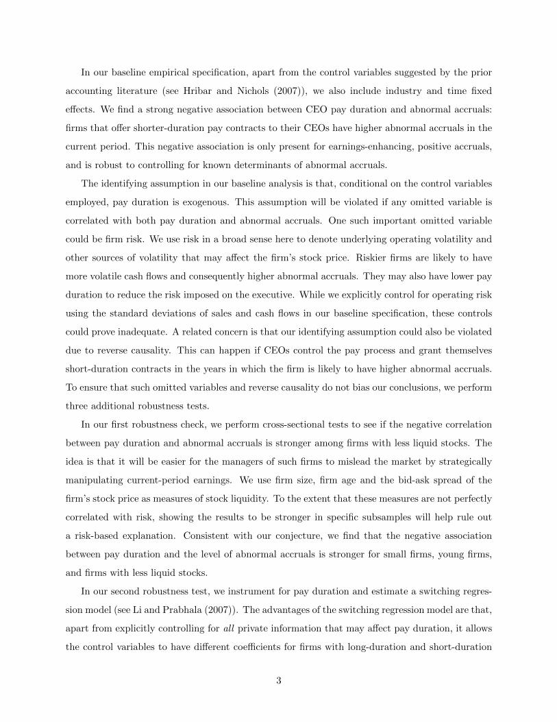
In our baseline empirical specification, apart from the control variables suggested by the prior

accounting literature (see Hribar and Nichols (2007)), we also include industry and time fixed

effects. We find a strong negative association between CEO pay duration and abnormal accruals:

firms that offer shorter-duration pay contracts to their CEOs have higher abnormal accruals in the

current period. This negative association is only present for earnings-enhancing, positive accruals,

and is robust to controlling for known determinants of abnormal accruals.

The identifying assumption in our baseline analysis is that, conditional on the control variables

employed, pay duration is exogenous. This assumption will be violated if any omitted variable is

correlated with both pay duration and abnormal accruals. One such important omitted variable

could be firm risk. We use risk in a broad sense here to denote underlying operating volatility and

other sources of volatility that may affect the firm’s stock price. Riskier firms are likely to have

more volatile cash flows and consequently higher abnormal accruals. They may also have lower pay

duration to reduce the risk imposed on the executive. While we explicitly control for operating risk

using the standard deviations of sales and cash flows in our baseline specification, these controls

could prove inadequate. A related concern is that our identifying assumption could also be violated

due to reverse causality. This can happen if CEOs control the pay process and grant themselves

short-duration contracts in the years in which the firm is likely to have higher abnormal accruals.

To ensure that such omitted variables and reverse causality do not bias our conclusions, we perform

three additional robustness tests.

In our first robustness check, we perform cross-sectional tests to see if the negative correlation

between pay duration and abnormal accruals is stronger among firms with less liquid stocks. The

idea is that it will be easier for the managers of such firms to mislead the market by strategically

manipulating current-period earnings. We use firm size, firm age and the bid-ask spread of the

firm’s stock price as measures of stock liquidity. To the extent that these measures are not perfectly

correlated with risk, showing the results to be stronger in specific subsamples will help rule out

a risk-based explanation. Consistent with our conjecture, we find that the negative association

between pay duration and the level of abnormal accruals is stronger for small firms, young firms,

and firms with less liquid stocks.

In our second robustness test, we instrument for pay duration and estimate a switching regres-

sion model (see Li and Prabhala (2007)). The advantages of the switching regression model are that,

apart from explicitly controlling for all private information that may affect pay duration, it allows

the control variables to have different coefficients for firms with long-duration and short-duration

3

pay contracts while at the same time permitting the estimation of interesting counterfactuals. Our

instruments for pay duration are the median pay duration of all CEOs in the same city as the firm

and the part of stock return that is due to market movement. Apart from the controls mentioned

above, we additionally include within-industry time fixed effects and abnormal stock return. Our

identifying assumption in the switching regression model is that the instruments are correlated with

pay duration, but conditional on duration and other controls employed, do not have an indepen-

dent effect on abnormal accruals. We believe that our instruments satisfy both these requirements.

Both instruments are statistically significant in the first-stage regression. We also believe that the

instruments satisfy the exclusion restriction: there is no a priori reason to expect the pay duration

of a neighboring CEO to affect the level of abnormal accruals of a firm after we control for com-

monality arising from industry affiliation. Furthermore, systematic movements in the stock price

should not affect the level of abnormal (or idiosyncratic) accruals, but they will affect pay duration

by changing the value of stock and option grants. Our estimates from the switching regression

model confirm our conclusion that firms that offer their CEOs shorter-duration pay contracts are

associated with higher abnormal accruals. The magnitude of the effect is greater in the switching

regression model as compared to the OLS model that we employ in our baseline analysis. This

indicates that reverse causality and the omitted variable bias are actually diminishing our OLS

estimates.

In our final robustness test, we introduce an alternative measure of managerial myopia. The

prior accounting literature shows that firms manage both their accounting earnings and real activity

so as to avoid reporting a loss (e.g., Burgstahler and Dichev (1997), and Roychowdhary (2006)).

We expect CEOs of firms with short-duration pay contracts to be particularly interested in avoiding

reporting a loss. Our tests confirm this conjecture. We find that CEOs with shorter-duration pay

contracts are more likely to manage both accounting earnings and real activities in order to avoid

reporting losses.

Summarizing, using the measure of pay duration developed in this paper, our empirical analysis

documents that firms that offer their CEOs shorter-duration pay contracts are associated with

higher abnormal accruals.

To examine the sensitivity of our results to the way we define pay duration, we develop an

alternative measure of pay duration and show that our results are robust to this alternative measure.

This measure differs from our baseline measure along two dimensions. First, it uses the pay-for-

performance sensitivities (PPS) of the stock and option grants, instead of the dollar values in

4

our baseline measure, as the weights to calculate the pay duration. We estimate PPS as the

change in the grant value corresponding to a 1% change in the firm’s stock price (Core and Guay

(2002)). Second, the calculation of duration with the alternative measure uses the executive’s entire

compensation portfolio, including all the prior year grants. We estimate the vesting schedules of

unvested prior year grants by looking at their year-on-year changes (see Section 2.1.3 for details).

This analysis raises an important question: If short-duration pay induces CEO myopia, why do

firms continue to offer such contracts in practice? That is, is there a benefit of short-term pay that

makes it optimal for certain firms? In the second part of the paper, we develop a theoretical model

that illuminates one possible benefit: shortening pay duration may improve the alignment of the

risk preferences of the manager and the firm’s shareholders.

Our model has several features that we believe reflect the real-world contracting environment.

The CEO controls the capital budgeting process and can affect both the length and the risk of

the firm’s projects. Long-term projects are more productive than short-term projects, and high-

risk projects have higher expected returns than low-risk projects. The first-best choice from the

risk-neutral shareholders’ perspective is the long-term, high-risk project, and shareholders design

the CEO’s incentive contract to maximize shareholder wealth. In the second-best case, however,

shareholders face a tradeoff between project duration and risk. On the one hand, exclusive reliance

on long-term compensation induces the CEO to choose the long-term project, but the CEO’s risk

aversion may result in her choosing inefficiently low risk. On the other hand, exclusive reliance on

short-term compensation causes the CEO to prefer the high risk that shareholders prefer but also

inclines the CEO to choose the short-term project. Shareholders optimize the second-best solution

by employing a mix of short-term and long-term pay to the CEO.

The model reveals that firms that have more valuable long-term projects and those that are

less risky offer their CEOs longer-duration pay contracts. To test this prediction, we use firm

size, Tobin’s Q, and R&D intensity to measure the duration of the firm’s projects. We find that

executive pay duration is longer in larger firms, firms with more growth opportunities, and in more

R&D-intensive firms. Consistent with our model’s prediction, we also find that riskier firms offer

shorter-duration pay contracts.

Our model predicts an ambiguous relationship between governance and executive pay duration.

In additional tests, we find empirical evidence consistent with this ambiguity. While pay duration is

shorter for executives in firms with a higher proportion of non-executive director shareholding, for

executives with more shareholdings in the firm, and in firms with lower entrenchment index values

5

(Bebchuck, Cohen, and Ferrel (2009)), it is longer in firms with a larger fraction of independent

directors on the board.

Our paper is related to the vast literature on executive compensation. The broader literature

has covered a wide-ranging set of issues.2 These include whether CEOs are offered sufficient stock-

based incentives and how these vary cross-sectionally,3 whether CEOs are judged using relative

performance evaluation (RPE),4 and ultimately whether executive contracts in practice are set by

the firm’s board of directors or the executives themselves.5

With respect to the duration of executive pay, there have been numerous theoretical contri-

butions, even going back as far as Holmstrom and Ricart i Costa (1986) who examine the pros

and cons of long-term compensation contracts in a managerial career-concerns setting. Examples

of other optimal contracting models that examine executive pay duration include Bizjak, Brickley,

and Coles (1993), Bolton, Scheinkman, and Xiong (2006), and Dutta and Reichelstein (2003). Em-

pirically, numerous papers have documented various features of CEO compensation. Walker (2011)

describes the evolution of stock and option compensation and the aggregate shift away from options

and toward restricted stocks. Core, Holthausen, and Larcker (1999), among others, have examined

the determinants of the cross-sectional variation in CEO compensation. Our marginal contribution

to this literature is that we develop a novel measure of pay duration that directly captures the mix

of short-term and long-term pay, and then use this measure to explain how pay duration varies in

the cross-section based on CEO and firm characteristics in a dataset that is much more detailed

than ExecuComp, and ultimately examine the effect of pay duration on corporate decisions.

Another important contribution of our work is that our duration measure is materially different

from the measures used in the prior literature to characterize executive pay, which include the pro-

portion of non-cash pay in total pay (Bushman and Smith (2001)), the delta and vega of executive

stock and option grants and holdings (Coles, Daniel, and Naveen (2006)), and the correlation of pay

to stock returns and earnings (Bushman et al (1998)).6 The key difference is that our pay duration

measure explicitly takes into account the length of the vesting schedule for each component of the

2We do not attempt to provide a thorough review here; the reader is referred to review papers like Frydman andJenter (2010), and Murphy (1999).

3See Aggarwal and Samwick (1999a), Garen (1994), Hall and Liebman (1998), Haubrich (1994), and Milbourn(2003).

4See Aggarwal and Samwick (1999b), Garvey and Milbourn (2003), Janakiraman, Lambert, and Larcker (1992),and Oyer(2004).

5See Bebchuk and Fried (2003), Bertrand and Mullainathan (2001), Garvey and Milbourn (2006), and Gopalan,Milbourn, and Song (2010).

6Much of this work has appeared in the accounting literature where researchers are also interested as to howincentive-based pay loads on both corporate earnings measures and the firm’s stock price. See also Banker and Datar(1989), Lambert and Larcker (1987), and Sloan (1993).

6

executive’s pay, of which there are often many during a given compensation year. This is important

because, for example, a large stock grant itself is unlikely to contribute to short-term incentives,

and this is particularly true if there is a long vesting schedule. Our empirical analysis confirms that

pay duration does a better job of predicting executive behavior than the coarser measures used in

the previous literature.

The rest of the paper is organized as follows. Section 2 describes our data and the empirical

methodology, and discusses the main results from a preliminary analysis of the data. Section 3

conducts a thorough empirical analysis relating pay duration and managerial myopia. Section 4

develops the model to understand the cross-sectional variation of pay duration, and draws out its

empirical predictions. Section 5 performs further empirical analysis to test the model’s predictions.

Section 6 concludes. All proofs and definitions of empirical variables are in the Appendix.

2 Data and Preliminary Empirical Analysis

In this section, we describe our data, construct the measures of pay duration, present the empirical

methodology, and provide the main results from a preliminary analysis of the data.

2.1 Data and descriptive statistics

We now describe our data sources, the categories of grants in the data, and the vesting schedules

of the grants.

2.1.1 Data sources

Our data come from four sources, Equilar, Execucomp, CRSP and Compustat:

• Data on the vesting schedules of restricted stock and stock options are drawn from Equilar

Consultants (hereafter, Equilar). Similar to S&P (provider of ExecuComp), Equilar collects

their compensation data from the firms’ proxy statements. We obtain details of all stock and

option grants to all named executives covered by Equilar for the years 2006-09.7 Equilar also

provides the grant date and the present value of the grants. The present value of a stock

grant is the product of the stock price on the grant date and the number of stocks granted,

while the value of an option grant is estimated by Equilar using the Black-Scholes formula.

7The sample of executives covered by Equilar is larger than that covered by S&P’s ExecuComp. Since we usedata from both sources, our final sample consists of executives covered by both datasets.

7

Equilar also identifies if either the size or the vesting schedule of the grant is linked to firm

performance.

• We obtain data on other components of executive pay, such as salary and bonus, from Exe-

cuComp. We carefully hand-match Equilar and ExecuComp using firm tickers and executive

names. Since prior studies on executive compensation predominantly use ExecuComp, we

ensure comparability of Equilar and ExecuComp by making sure the total number of options

granted during the year for each executive in our sample is the same across the two datasets.

• We complement the compensation data with stock returns from the Center for Research in

Security Prices (CRSP) and firm financial data from Compustat.

2.1.2 Various categories of grants

In practice, the specific terms of stock and option grants are quite complex. Both the number

of securities granted and the vesting schedule can depend on future firm performance. For our

analysis, we classify the grants into three categories; see Table 1 for the distribution of our sample

grants across the three categories. The first category is the simplest. It includes grants where the

number of securities offered is fixed as of the grant date, and the grant has a time-based vesting

schedule. Of the total 37,304 (25,738) stock (option) grants in our sample, 21,999 (24,531) or

58.97% (95.31%) belong to this category. For each grant in this category, we have information on

the size of the grant, the length of the vesting period (i.e., the time by when the grant is completely

vested) and the nature of the vesting, i.e., whether the grant vests in equal installments over the

vesting period (graded vesting) or entirely at the end of the vesting period (cliff vesting).

The next category includes grants for which the number of securities offered is fixed as of

the grant date but the vesting schedule is contingent on future firm performance. Of all the

grants in our sample, 5.73% (2.79%) of the stock (option) grants belong to this category. For

such grants, Equilar records the grant size, the period over which performance is measured and

the performance metrics used. We assume that these grants vest all at once at the end of the

performance-measurement period. Also, for grants with a performance-linked accelerated vesting

schedule, we assume that they vest according to the initially-specified vesting schedule. We rely

on this approximation because the acceleration provisions in these grants are usually very complex

and depend on multiple performance measures. Thus, it is not at all straightforward to determine

if and when these grants will vest on an accelerated basis.

8

The third group of grants are part of long-term incentive plans in which the number of securities

awarded is contingent on future performance. Some of these grants are also associated with a time-

based vesting schedule for tax purposes (see Gerakos, Ittner, and Larcker (2007)). For such grants,

Equilar records the target number of securities expected to be granted, the period over which

performance is measured and any time-based vesting schedule associated with the grant. Of all the

stock (option) grants in our sample, 35.25% (1.88%) belong to this category. We include all these

grants in calculating our duration measure, with the number of securities used in the calculation

being the target number of securities to be granted. To estimate the vesting schedules of these

grants, we assume that the vesting starts right after the performance measurement period.

We are not able to identify either the performance-measurement period or the vesting period

for 23 grants in our sample. They are categorized as other grants and excluded from our analysis.

We do not specifically differentiate between time-based and performance-based vestings; see Bettis

et al (2010) for a detailed discussion of grants with performance-based vesting.

[Table 1 goes here]

2.1.3 Vesting schedules of pre-2006 grants

Although our analysis focuses on the years 2006-09, obtaining a comprehensive measure of pay dura-

tion for that period requires that we estimate the vesting schedules of unvested pre-2006 (excluding

2006) stock and option grants in the executive’s compensation portfolio. We use ExecuComp to

estimate the vesting schedules of these grants. For every executive, ExecuComp provides details on

the total outstanding unvested stock and option grants at the end of each year, and then aggregates

the option grants into groups with the same exercise price and expiration date. For option grants,

our estimation procedure involves the following steps:

1. We first aggregate the outstanding unvested post-2006 option grants (2006 included) from

Equilar into unique exercise price-expiration date pairs, and merge Equilar and ExecuComp

using executive identity, year, exercise price and expiration date.

2. We then subtract the unvested post-2006 grants from the total outstanding grants (which we

get from ExecuComp) to isolate the unvested pre-2006 grants.

3. We use the year-on-year change in the outstanding unvested pre-2006 grants to estimate their

vesting schedule. We can do this for all grants except those that remain unvested at the end

9

of 2010: there are 2,177 such grants for 1,272 executive-years (3.6% of our sample) in our

sample. We assume that these grants vest at the end of 2011. We check the robustness of

our conclusions by repeating our tests after excluding these executive-years.

We follow the same procedure to approximate vesting schedules of unvested pre-2006 stock grants,

except that we match Equilar and ExecuComp using just executive identity and year (since a

restricted stock has no expiration date or exercise price).

2.2 Measures of pay duration

In this subsection, we introduce our measures of executive pay duration involving both restricted

stock and option grants.8

2.2.1 Baseline measure

Our baseline measure is constructed using only the data on post-2006 awards provided by Equilar.

We follow the fixed income literature and calculate pay duration as the weighted average duration

of the four components of pay (i.e., salary, bonus, restricted stock, and stock options). In cases

where the stock and option awards have a cliff vesting schedule, we estimate pay duration as:

Duration =

(Salary +Bonus)× 0 +ns∑i=1

Restricted stocki × ti +no∑j=1

Optionj × tj

Salary +Bonus+ns∑i=1

Restricted stocki +no∑j=1

Optionj

, (1)

where the subscript i denotes a restricted stock grant and the subscript j denotes an option grant.

Salary and Bonus are, respectively, the dollar values of annual salary and bonus. We calculate du-

ration relative to the year end, so Salary and Bonus have a vesting period of zero. Restricted stocki

is the dollar value of restricted stock grant i with corresponding vesting period ti in years. During

the year, the firm may have other stock grants with different vesting periods (different ti), and

ns is the total number of such stock grants. Optionj is the Black-Scholes value of option grant j

with the corresponding vesting period tj in years; no has a similar interpretation as ns. In cases

8Cadman, Rusticus, and Sunder (2010) also introduce a similar measure of pay duration, but use only the vestingschedule of stock options. Thus, their measure only estimates the duration for the option component of pay. Since weinclude both stock options and restricted stock and estimate the duration for the entire compensation package, ourmeasure is more comprehensive. Chi and Johnson (2009) examine the effect of CEO incentive horizon on firm value,but they only look at the amount of vested stock and option grants relative to unvested ones without estimating ameasure of pay duration.

10

where the restricted stock grant (option grant) has a graded vesting schedule, we modify the above

formula by replacing ti (tj) with (ti + 1)/2 ((tj + 1)/2).9

2.2.2 Alternative measure of pay duration

Our baseline measure of pay duration does not include grants from prior years. To account for

that, we construct our alternative measure by expanding the estimation in (1) to include all stock

and option holdings and grants from prior years. For each year during 2006-09, we include: (i) all

vested stock and option holdings awarded from all prior years (for which we assign a vesting period

of zero), (ii) unvested pre-2006 grants (for which we follow the procedures outlined in Section 2.1.3

to estimate the vesting schedules), and (iii) unvested post-2006 grants (for which we have detailed

information on vesting schedules from Equilar).

The second change we make in constructing the alternative measure is to use the pay-for-

performance sensitivity (PPS) of the stock and option grants, instead of their dollar value, as the

weight to calculate the pay duration.10 We follow Core and Guay (2002) and calculate PPS as

the change in the grant’s value corresponding to a 1% change in the firm’s stock price. We then

combine the PPS and the vesting schedules to calculate the alternative pay duration as:

DurationPPS, total =

ns∑i=1

tsi∑t=0

PPSSi,t × t+no∑j=1

toj∑t=1

PPSOj,t × t

ns∑i=1

PPSSi +no∑j=1

PPSOj

. (2)

In (2), the subscript i denotes a restricted stock grant and the subscript j denotes an option grant.

PPSSi,t is the PPS of the portion of stock grant i that vests in t years; tsi is the final vesting period

of stock grant i, and ns denotes the total number of stock grants, which equals two plus the number

of stock grants from Equilar.11 PPSSi denotes the aggregate PPS of the restricted stock grant i.

Similarly, PPSOj,t is the PPS of the portion of option grant j that vests in t years; toj is the final

vesting period of option grant j, and no denotes the total number of option grants, including: (i)

9To see this, consider a stock grant i′ that vests equally over ti′ years. Since a fraction 1/ti′ of the grant is vested

each year, the term Restricted stocki′ × ti′ in (1) should be replaced by Restricted stocki′ ×(

1ti′

+ 2ti′

+ . . .+ti′ti′

)=

Restricted stocki′ti′

× ti′ (ti′+1)

2= Restricted stocki′ ×

(ti′+1

2

). Optionj × tj can be modified in the same way.

10We thank an anonymous Associate Editor for suggesting that we use PPS in constructing an alternative durationmeasure.

11This is because apart from the post-2006 stock grants from Equilar, we also include: (i) all the vested stock grants(as the first additional count), for which we assign a vesting period of zero, and (ii) the aggregate unvested pre-2006stock grants (as the second additional count), whose vesting schedules are approximated using the procedures outlinedin Section 2.1.3.

11

post-2006 option grants from Equilar, (ii) the aggregate vested pre-2006 option grants, and (iii) the

unvested pre-2006 option grants aggregated into groups with the same exercise price and expiration

date. PPSOj denotes the aggregate PPS of option grant j.

We also construct another alternative measure, DurationPPS, award, which is similar toDurationPPS, total,

but includes only annual grants for each year during the period 2006-09, i.e., it does not include

grants from prior years. We use this as a control variable in some of our tests.

2.2.3 Discussion

Our measure of pay duration has several advantages over the measures used in the prior literature

to characterize executive pay. A principal objective of all these measures is to understand the mix

of short-term and long-term pay and hence the extent to which overall pay provides short-term

incentives to executives. These existing measures include the proportion of stock and option grants

(non-cash pay) in total pay, the delta and vega of the executive’s stock and option holdings, and the

correlation of executive pay with stock returns and accounting earnings. The important difference

between pay duration and those measures is that duration explicitly accounts for the length of the

vesting schedules of the stock and option grants. Clearly, a large stock grant itself is unlikely to

contribute to short-term managerial incentives if it has a long vesting schedule. While the delta

and vega of an executive’s compensation portfolio capture its sensitivities to movements in stock

price and its volatility, respectively, they do not capture the mix of short-term and long-term

incentives in the pay contract, which our measure does. And, unlike the correlation measure, we

directly measure the mix of short-term and long-term pay in computing pay duration. Finally,

our empirical analysis later confirms that our duration measure does a better job in predicting

executive behavior than those existing measures.

Our measure does have some limitations. First, we do not include severance and post-retirement

benefits that may be important for providing long-term incentives. The main reason for this

exclusion is the difficulty in obtaining the vesting schedules of these benefits. Despite this, in our

subsequent empirical analysis we find that pay duration is significantly associated with measures of

myopic behavior such as the level of abnormal accruals. This association survives controls for the

extent of deferred compensation. A second important limitation of our measure (as we explained in

Section 2.1.2) is that we ignore the optionality introduced by linking both the size and the vesting

schedule of the grant to future firm performance.

12

In employing our definition of duration to capture the extent of short-term and long-term pay,

we implicitly assume that other than the vesting schedule, there are no other restrictions, either

explicit or implicit, on the executive’s ability to exercise and sell the stock and option grants as

soon as they vest. To the extent that such restrictions exist, pay duration will be a noisy proxy

that underestimates the extent of long-term incentives provided to the executive. Assuming that

these restrictions are randomly distributed, they are likely to add noise to duration as a measure of

managerial investment horizon and thus bias our estimates downward. Even if the restrictions are

systematically correlated with accruals – firms with such restrictions have lower abnormal accruals

– by not taking these restrictions into account, pay duration will underestimate the investment

horizon of the executives and thus bias against finding the hypothesized relationship between CEO

pay duration and abnormal accruals.

2.3 Empirical specification and key variables

In this section, we discuss our empirical specification as well as our robustness checks.

2.3.1 Baseline regression

In our main empirical analysis, we estimate how CEO pay duration affects her choice of investment

horizon. We achieve this by estimating variants of the following OLS model:

ykt = α+ β1 ×Durationket + β2Xkt + µtT + µiI + εkt, (3)

where the subscript k indicates the firm, e the CEO, t time in years, and i the firm’s three-digit

SIC industry. The terms T, I and Xkt refer to, respectively, a set of year dummies, three-digit SIC

industry dummies and firm characteristics. The variable y is a measure of investment horizon. In

much of our analysis, y represents signed abnormal accruals, Accruals. A larger value of Accruals

implies higher earnings in this period relative to cash flows. Since signed accruals must sum up

to zero in the long-run, larger accruals in the current period imply a lower level of accruals and

consequently lower earnings in future periods. Thus, managers can use “discretionary accruals” to

shift income across time periods. We calculate Accruals following the procedure outlined in Jones

(1991), modified by including controls for earnings performance as proposed in Kothari, Leone,

and Wasley (2005). In some of our tests, we split Accruals into positive and negative accruals to

13

shed further light on the mechanism at work. The standard errors in our regressions are robust to

heteroskedasticity and are clustered at the three-digit SIC code industry level.

Our sample for these regressions includes one observation per firm-year. Our choice of control

variables is guided by the prior accounting literature (see, for example, Hribar and Nichols (2007)).

To control for differences in firm size, we include Log(Total assets) and Log(Market cap), the

natural logarithm of the firm’s book value of total assets and market capitalization, respectively.

We control for growth opportunities using the market-to-book ratio (Market to book) and annual

sales growth (Sales growth), for profitability using Cashflows, for operating volatility using the

standard deviations of cash flows and sales (S.D. Cashflow and S.D. Sales, respectively), and for

leverage using DebtTotal assets (the ratio of total debt over total assets). We also include industry and

time fixed effects, and only rely on within-industry differences in the level of accruals for our

identification.

The identifying assumption in (3) is that conditional on all the control variables employed,

Duration is exogenous. This allows us to interpret the coefficient on Duration as a measure of

the causal effect of pay duration on abnormal accruals. Our assumption will be violated if any

omitted variable is correlated with both Duration and Accruals. One such important omitted

variable could be firm risk. Riskier firms – those with more volatile operating performance – may

have higher abnormal accruals as they try to smooth accounting earnings over time. Such firms

may also have shorter pay durations, for example, because pay uncertainty increases the cost of

long-term compensation.

We employ two methods in our baseline model to control for such risk differences. First, in

calculating Accruals, we isolate the discretionary portion of accruals. We calculate Accruals as

the residuals from regressing total accruals on firm size, firm growth and asset structure. We

run this regression individually for every industry-year. This ensures that Accruals measures only

deviations from the industry average. Second, we explicitly control for operating risk using the

standard deviations of sales and cash flows in our baseline model.

However, one could still argue that these two steps may not be enough. Specifically, unobserved

risk differences could bias our conclusions. Further, the identifying assumption in our baseline

model could also be violated due to reverse causality. This can happen if CEOs control the pay

process and grant themselves a short-duration contract especially in the years when the firm is

14

likely to have higher abnormal accruals.12 To deal with such a potential omitted-variable bias and

reverse causality, we perform three additional tests, which are discussed below.

2.3.2 Methodologies for robustness check

For our first robustness check, we observe that if higher Accruals among firms with short CEO

pay duration reflect managerial effort to boost the short-term stock price, then this should be

more prevalent among firms with less liquid stock. Such firms will have less scrutiny in the public

equity market, making it easier for the manager to manipulate the stock price by reporting high

short-term earnings. To test this conjecture, we conduct cross-sectional tests differentiating firms

based on size, age and bid-ask spread. These tests help our identification because any competing

risk-based explanation must not only fit our baseline estimates, but also explain why the results

are stronger in specific subsamples. Moreover, if the board of directors serves a monitoring role to

limit managerial myopia, then the effect of pay duration on Accruals should be stronger for firms

with weaker board oversight. We use the extent of non-executive director shareholding as a proxy

for board oversight to test this.

In our second robustness test, we use a switching regression model to explicitly control for pri-

vate information that may be correlated with pay duration (see Li and Prabhala (2007)). We do

this by instrumenting for Duration using the median duration of all CEOs in the same city as the

firm’s CEO (City duration) and the part of stock return due to market movement (Expected return).

The advantages of the switching regression model are that, apart from explicitly controlling for all

private information that may affect pay duration, it allows the control variables to have coefficients

for firms with long-duration pay that differ from those with short-duration pay, while at the same

time enabling us to estimate interesting counterfactuals. Apart from the controls mentioned above,

we also include abnormal returns, Abnormal return, and within-industry time fixed effects in this

model. Our identifying assumption for the switching regression model is that the two instruments

are correlated with Duration, but not related to Accruals conditional on Duration and the other

controls employed (i.e., the exclusion restriction). We believe our instruments satisfy both require-

ments. First, both instruments are statistically significant in the first-stage regression, where the

dependent variable is Duration. We also believe that the instruments satisfy the exclusion restric-

tion for the following reasons. Given that we control for within-industry time fixed effects, there

12Note that this explanation does not invalidate the assumption that a short-duration pay contract allows themanager to exploit short-term stock mispricing arising from higher accruals.

15

is no a priori reason to expect a relationship between the pay duration of a neighboring CEO and

the level of abnormal accruals of a firm. We also believe the portion of stock return due to market

movement should be uncorrelated with abnormal accruals that are calculated net of an expected

level of accruals based on firm and industry characteristics.

For our third robustness check, we test whether our results are robust to alternative measures

of managerial myopia. The prior literature shows that managers are reluctant to report losses.

This can be seen from the abnormally high (low) fraction of firms with small positive (negative)

earnings (Burgstahler and Dichev (1997)). There is also evidence that managers manipulate both

real investment activity (Roychowdhury (2006)) and accruals (Burgstahler and Dichev (1997)) in

order to avoid reporting losses. We expect the loss-reporting-avoidance incentives to be stronger

for executives with shorter pay durations. We test this to further establish how pay duration affects

the manager’s investment horizon.

2.4 Summary statistics and univariate analysis

We now present the summary statistics for the distribution of vesting schedules, the industry

distribution of pay duration, and the key variables in the analysis. We also present the results of our

univariate analysis that examines how pay duration is related to executive and firm characteristics.

2.4.1 Distribution of vesting schedules

In Panel A of Table 2, we provide the distributions of the vesting periods for restricted stock and

option grants for all executives in our sample. The distributions are somewhat similar for stocks

and options, although a chi-squared test rejects the null that the two are identical. The vesting

periods cluster around the three to five-year horizon for both stocks and options and a large fraction

of the vesting schedules are graded. In Panel B, we provide the distributions of the vesting periods

just for CEOs (identified by the CEOANN field in ExecuComp). The distributions are similar to

those in Panel A for all executives. For both stocks and options, we find that the distributions of

vesting periods for CEOs first-order stochastic dominate (FOSD) those for all other executives. This

suggests a longer pay duration for CEOs, which is confirmed later by our univariate evidence. Note

that while in Tables 1 and 2 we include all the stock and option grants for which we have vesting

schedules from Equilar, our sample in subsequent tables is confined to executive-years for which we

are able to exactly match the number of annual option grants across Equilar and Execucomp.

16

[Table 2 goes here]

2.4.2 Industry distribution of pay duration

Table 3 provides the industry distributions of Duration and DurationPPS, total for CEOs and all

executives in our sample. We use the Fama-French 48 industry classification and report the average

pay duration of all executives and CEOs in separate columns within each industry. We include all

industries with pay duration information for at least five executives. For ease of reference, we sort

the data in terms of decreasing Duration for CEOs. We find that industries that have assets with

longer duration (e.g., Defense, Electrical Equipment, and Coal) are also those that have longer

executive pay duration (for CEOs and for all executives). We also find that DurationPPS, total

is consistently lower than Duration. This is because DurationPPS, total includes both vested and

unvested grants from prior years that have shorter remaining vesting periods.

It is interesting to note that executives in the Finance-Trading industry (e.g., securities broker-

dealers) have relatively long pay durations on average; they rank 11th among the 48 industries.13

This evidence seems to be at odds with the notion of excessive short-termism in executive com-

pensation for financial services firms. In fact, the relatively long pay duration in these firms may

reflect recognition by the boards of directors of these firms that it is relatively easy for the CEOs

to alter the portfolios of their firms to boost the short-term stock price, so a longer pay duration

must be used to counteract this propensity.

[Table 3 goes here]

2.4.3 Summary statistics of key variables

Panels A and B of Table 4 provide, respectively, the summary statistics of the key variables used

in our analysis for all executives and for CEOs in our sample. Focusing on Panel A, we find that

the average annual total compensation for our sample executive is $2,214,425, which consists of

$447,365 of salary, $143,252 of bonus, $908,969 of stock options, and $711,228 of restricted stocks.

These numbers are comparable to those reported in previous studies. The average executive pay

duration in our sample, measured by Duration, is 1.218 years. Thus, executive pay vests, on

average, about one year after it is granted. In comparison, the average value of DurationPPS, total

13It is also interesting to note that Banking firms (e.g., depository institutions) have shorter average executive payduration than firms in the Finance-Trading industry.

17

in our sample is 0.61 years. Our sample tilts towards larger firms in Compustat, as shown by the

median value of total assets of $2,195 million.

Our next set of variables measure the corporate governance characteristics of the sample firms.

As for the shareholding of non-executive directors (Director shareholding), the average is 2.334%,

whereas the median is less than 1%; note that ExecuComp records director shareholding less than

1% as zero. The average Bebchuk, Cohen, and Ferrell (2009) entrenchment index of our sample

firms is about 3 (out of 6), and the average fraction of independent directors on our sample firms’

boards (Fraction independent) is 76.3%. The average executive in our sample holds about 0.642%

of the firm’s shares (Shareholding), and is 52 years old. The average level of Accruals in our sample

is 0.002.

In Panel B, we present the summary statistics for the subsample of CEOs. Comparing with

Panel A, we find that, as expected, the CEOs in our sample have a higher annual total compensation

than the average executive ($4,841,917 vs. $2,214,425). This higher compensation is reflected in

four pay components (salary, bonus, options, and restricted stock). The pay duration, measured by

Duration, is also longer for the CEO than for the average executive (1.44 years vs. 1.218 years).

Interestingly, we find that the average CEO has a lower DurationPPS, total as compared to the

average executive (0.456 years vs. 0.61 years). This is because of a large amount of vested stock

and option grants in the average CEO’s compensation portfolio. The average CEO is 55 years old,

and holds more shares in the firm than the average executive (2.239% vs. 0.642%). To reduce

the effects of outliers, our variables of empirical interest are all winsorized at the 1% level and we

estimate standard errors that are robust to heteroskedasticity throughout our analysis.

[Table 4 goes here]

2.4.4 Univariate test

In this subsection, we present the findings of our univariate analysis of the relationship of pay

duration to executive and firm characteristics. In Panel A of Table 5, we split our sample into

executives with above and below median pay duration as measured by Duration (the difference

in Duration across the subsamples is 1.595 years), and compare the characteristics across the two

subsamples. Executives with above-median pay duration have a higher annual total compensation,

which is reflected in three components of pay, but most starkly in the values of option and restricted

stock grants. Interestingly, executives with longer-duration pay contracts receive about $62,523

18

less bonus on average. Pay duration is longer among larger firms (shown by the difference in Total

assets). Firms awarding longer-duration pay contracts have higher sales growth (7.5% vs. 6.2%),

higher market-to-book ratios (1.838 vs. 1.601) and higher R&D expenditures as a proportion of

total assets (2.5% vs. 2.2%). These indicate that firms that are growing faster and have more

growth opportunities offer longer-duration pay contracts. Executives with longer pay duration are

from firms that are more profitable (measured by EBITSales ), have lower stock volatility, and have

greater stock liquidity as reflected in a lower bid-ask spread.

Focusing on the governance characteristics, we find that firms that offer longer-duration pay

contracts have higher entrenchment index values and lower shareholdings by both non-executive

directors and executives. If larger shareholdings of non-executive directors and executives and a

lower entrenchment index value signify firms with better governance, then these results suggest

that better-governed firms offer shorter-duration pay contracts. However, firms that offer longer-

duration pay contracts also have higher proportions of independent directors. So, if a higher

proportion of independent directors signifies a more independent board, then this conflicts with the

idea that better-governed firms offer shorter-duration pay contracts. We also find that executives

with longer pay duration are younger on average. Finally, firms that offer longer-duration pay

contracts have higher abnormal accruals. Since these are univariate comparisons, we do not control

for the other firm-level determinants of Accruals.

In Panel B, we confine our comparisons to the subsample of CEOs. We only examine pay and

executive characteristics as the comparisons of firm characteristics are similar to those in Panel A.

We find that CEOs with longer pay durations have significantly higher annual total compensation

as well as higher pay along three subcategories: salary, restricted stock, and options. CEOs with

longer-duration pay contracts have significantly lower bonus and lower shareholdings on average,

and are younger.

In Panel C of Table 5, we split our sample into executives with above and below median

DurationPPS, total, and compare the two subsamples. It is immediately evident from Panel C that

the two subsamples here are more similar to each other than the two subsamples presented in

Panel A. DurationPPS, total is affected by both the vesting schedule of the annual pay contract

and the executive’s decision to exercise and sell vested stock and option grants. To the extent the

latter decision depends on idiosyncratic executive characteristics, the difference in the nature of

the pay contract and firm characteristics between executives with above-median and below-median

DurationPPS, total will be lower than the corresponding difference between executives with above-

19

median and below-median Duration. Executives with longer DurationPPS, total have higher annual

total compensation, which is mainly driven by more restricted stock grants. Executives with longer

DurationPPS, total actually have lower salary, bonus and option grants, on average.

There is no significant difference in firm size across the two subsamples, but executives with

longer DurationPPS, total manage firms with higher leverage (measured by DebtTotal assets). Firms with

longer executive DurationPPS, total have lower sales growth, lower market-to-book ratios, lower

R&D expenditures (as a proportion of total assets), but higher capital expenditures. Thus, there

does not appear to be a consistent relationship between DurationPPS, total and growth opportu-

nities. Executives with longer DurationPPS, total are from firms that are less profitable, and from

firms with higher stock volatility and more liquid stocks (as manifested by lower bid-ask spreads).

Focusing on the governance characteristics, we find that firms with longer executiveDurationPPS, total

have lower shareholdings by both non-executive directors and executives (signifying weak gover-

nance), but are associated with a higher proportion of independent directors (signifying good gov-

ernance). There is no significant relationship between DurationPPS, total, the entrenchment index

and the level of abnormal accruals. We also find that executives with longer DurationPPS, total are

younger.

Panel D confines the comparisons to CEOs. Here again, we only examine pay and executive

characteristics, since the comparisons of firm characteristics are similar to those in Panel C. We

find that CEOs with longer DurationPPS, total are younger, and have significantly higher annual

total compensation (mainly driven by restricted stock grants) and lower shareholdings.

[Table 5 goes here]

3 Pay Duration and Managerial Myopia

In this section, we examine the effect of pay duration on managerial behavior. We first perform

baseline regressions, with a host of control variables, that explore the relationship between pay

duration and managerial myopia, as reflected in an emphasis on the use of accruals to boost short-

term earnings. We then perform three robustness checks to deal with the potential violation of our

assumption that pay duration is exogenous. We end the section with an analysis of the robustness

of our results to an alternative definition of pay duration.

20

3.1 Results from baseline regressions

In Panel A of Table 6, we relate CEO pay duration to the level of signed abnormal accruals, Accruals.

Our specification in these tests follows Hribar and Nicholas (2007). The results in Column (1) show

that firms that offer longer-duration pay contracts to their CEOs are associated with lower levels

of abnormal accruals. The coefficients on the control variables indicate that firms with higher

market-to-book ratios (positive coefficient on Market to book), less volatile cash flows (negative

coefficient on S.D. Cashflow), more volatile sales (positive coefficient on S.D. Sales), lower cash

flows (negative coefficient on Cashflows), higher sales growth (positive coefficient on Sales growth)

and higher market capitalization (positive coefficient on Log(Market cap)) have higher abnormal

accruals. Note that the R2 in our regression, 28.6%, is influenced by the inclusion of industry and

time dummies. In Column (2), we repeat our estimates after controlling for the fraction of the

executives’ shareholding and find our results to be robust.

In Columns (3) and (4), we split Accruals into positive and negative accruals and repeat our

estimation. Specifically, our dependent variable in Column (3) is Accruals×Positive accruals (where

Positive accruals is a dummy variable that identifies firm-years with positive abnormal accruals),

while the dependent variable in Column (4) is Accruals × (1 − Positive accruals). Bergstresser

and Philippon (2006) show that the sensitivity of CEO pay to stock price movements affects the

executive’s incentive to manage earnings. We control for that by including the natural logarithm

of the delta of the CEO’s stock and option portfolio, Log(Delta). We measure Delta using the

procedure in Coles, Daniel, and Naveen (2009). Our results indicate that pay duration is negatively

related to positive accruals. We do not find a significant relationship between pay duration and

negative accruals. This indicates that a longer-duration pay contract reduces the CEO’s incentive

to engage in earnings-enhancing accruals.

Apart from a long vesting schedule, executives can also be given long-term incentives through

deferred compensation. To see if the effect of Duration on Accruals is robust to controlling for

the extent of long-term incentives provided by such deferred compensation, in unreported tests we

repeat our estimations after controlling for the extent of deferred pay using High deferred pay, a

dummy that identifies executives with above median value of deferred compensation as a fraction

of total compensation. We obtain results similar to those reported here.

Summarizing, our results in Panel A show that firms that offer their CEOs longer-duration pay

contracts are associated with lower levels of accruals and more specifically, less positive accruals,

21

which is consistent with the intuition that short-duration pay provides incentives for managers to

emphasize short-term earnings. Our results are economically significant as well. Comparing the

coefficient in Column (3) to the mean value of positive accruals in our sample, we find that a one

standard deviation increase in Duration (0.967 years) leads to an 8% reduction in the extent of

positive accruals as compared to its sample mean.

3.2 Robustness checks

As indicated earlier, because of the possibility of violation of our baseline-regression assumption

that pay duration is exogenous, we perform three robustness checks. These are: (i) an examination

of whether the effect of pay duration on managerial myopia is stronger for firms that are smaller,

younger, have less liquid stocks, and weaker board oversight; (ii) a switching regression model to

control for endogeneity; and (iii) the use of an alternative measure of managerial myopia. We show

that our results survive all of these robustness checks.

3.2.1 First robustness check: linking the effect of pay duration on managerial myopia

to firm size, age, stock liquidity and governance

In Panel B of Table 6, we test our cross-sectional predictions by repeating our tests in different

subsamples. In Columns (1) and (2), we divide our sample into small and large firms and repeat

our tests. We identify firms as small if they have below-sample-median market capitalization. Our

results indicate that while Duration is negatively related to Accruals both for small and large

firms, the absolute value of the coefficient for small firms is twice the size of that for large firms.

The economic magnitude of the effect is also greater for small firms, because the mean value of

absolute Accruals is lower for small firms as compared to that for large firms (0.0002 vs. 0.0035).14

In Columns (3) and (4), we divide our sample based on bid-ask spread. Our results indicate that

Duration has a statistically significant effect on Accruals only for firms with above median bid-ask

spreads. In Columns (5) and (6), we divide our sample into young and old firms. We classify

firms as young if they have below-median firm age, where firm age is the number of years since the

IPO year. Since older firms are likely to have greater institutional shareholding (Bennett, Sias, and

Starks (2003)), we expect duration to have a greater affect on accruals for younger firms. Consistent

with this, we find Duration has a significant effect on Accruals only for young firms. Finally, in

14We compare the coefficient with the mean value of absolute accruals because signed accruals tend to have anaverage close to zero.

22

Columns (7) and (8) we repeat our tests in subsamples of firms with high and low board oversight.

We classify firms in which non-executive directors own more than 1% of the shares as having better

board oversight. Again, we find that the negative correlation between Duration and Accruals is

present only in the subsample of firms with weak board oversight.

Overall, our results in Panel B show that the effect of Duration on Accruals is greater for

smaller firms, younger firms, firms with less liquid stocks, and firms with weak board oversight.

When we repeat our tests using Short duration instead of Duration, where Short duration identifies

firms with below median CEO pay durations, we obtain results similar to the ones reported here.

These results provide strong evidence that pay duration affects the manager’s investment horizon.

[Table 6 goes here]

3.2.2 Second robustness check: switching regression model to control for endogeneity

We now perform tests that explicitly control for private information that may affect pay duration

and abnormal accruals. In particular, we wish to deal with the possibility that the manager may

possess private information about impending high abnormal accruals and may therefore choose a

short-duration contract to take advantage of it. In Panels A and B of Table 7, we relate Accruals

to CEO pay duration after controlling for endogeneity. To do this, we first convert our main inde-

pendent variable, Duration, into a dummy variable, Short duration, which takes the value one for

CEOs with below sample-median pay duration as measured by Duration. To control for endogene-

ity, we estimate a switching regression model (see Fang (2005), and Li and Prabhala (2007)). The

model consists of estimating three regressions: a probit selection model with Short duration as the

dependent variable, and two separate OLS models with Accruals as the dependent variable that

are estimated for firms with below-median and above-median CEO pay duration.15 We augment

the two OLS models with the Inverse Mills ratio and the Mills ratio, respectively, estimated from

the first-stage regression.16

In Column (1) of Panel A, we present the results of the first-stage probit model. We use two

exogenous instruments for pay duration. Our first instrument is the median Duration of all CEOs

15The switching regression model, while similar to a Heckman selection model, is more general because it estimatestwo second-stage equations and thus allows for different coefficients on the covariates for the “selected” and the“not-selected” samples. Similar to the Heckman model, the identification comes from the non-linearity of the model,which arises from the assumption of joint normality for the error terms.

16The Mills ratio and the Inverse Mills ratio are given by the formulas φ(γZ′)Φ(γZ′) and −1×φ(γZ′)

1−Φ(γZ′) , where φ and Φdenote, respectively, the probability density function and the cumulative distribution function of the standard normaldistribution, Z is the vector of regressors used in the selection model, and γ denotes the vector of coefficient estimatesfrom the selection model.

23

of firms in the same city as the CEO (see Hochberg and Lindsey (2010) for a similar idea), City

duration. Our second instrument is Expected return, which is the part of stock return due to

market movements. We believe these instruments satisfy the two requirements necessary for our

identification. First, we believe City duration will be correlated with Duration through local peer

effects. CEOs are likely to meet each other socially and exchange information on the structure of

their compensation contracts. Such interaction is also likely at the board level. These may lead

to geographic clustering in the structure of compensation contracts. Apart from Hochberg and

Lindsey (2010), Shue (2011) also documents peer effects in the structure of CEO compensation.

These studies offer support for why City duration will be correlated with Duration. To ensure

that this relationship is not due to industry similarity, we include within-industry time effects in

our regressions. By changing the value of stock and option grants, Expected return, is also likely

to affect Duration.17 We believe our instruments also satisfy the exclusion restriction. There is

no a priori reason to expect the duration of a neighboring CEO (of a firm in the same city) to

affect the level of abnormal accruals. We also believe the portion of stock return due to market

movements should be uncorrelated with abnormal accruals that are net of expected accruals. The

Jones (1991) model that we employ is designed to estimate expected accruals using industry and

firm characteristics. Since idiosyncratic movements in the stock price may be correlated with

Accruals, we include Abnormal return (part of stock return not due to market movement) as an

additional control in our regression.

Apart from the exogenous instruments, we also include all observable firm and executive char-

acteristics that may affect duration and also the level of accruals. We confine this regression to

firms in cities with a minimum of three firms. The coefficients in Column (1) indicate that the

median pay duration of CEOs in the same city is significantly negatively related to Short duration.

We also find that firms with higher Expected return have longer pay duration. Firms with higher

market-to-book ratios, lower leverage, more volatile sales, and lower abnormal returns in the recent

past have shorter-duration pay contracts. We find that firm size has an ambiguous effect. While

the coefficient on Log(Total assets) is positive, that on Log(Market cap) is negative and significant.

In Columns (2) and (3), we present the results of the OLS regressions with Accruals as the

dependent variable for firms with below-median CEO pay durations (Column (2)) and those with

above-median CEO pay durations (Column (3)). The empirical specification in these columns is

similar to that in Column (1) in Panel A of Table 6, except that we include the Inverse Mills

17We thank an anonymous Associate Editor for suggesting this instrument.

24

ratio and Mills ratio as additional regressors in Columns (2) and (3), respectively, to control

for unobserved characteristics (i.e., private information) that may affect both pay duration and

Accruals. A test of whether Accruals is higher for firms with below-median CEO pay duration is

to compare the actual level of Accruals for such firms with the counterfactual level of Accruals if

the same firms had above-median pay duration. We estimate the counterfactual by combining the

coefficient estimates in Column (3) with the firm and executive characteristics for firms with below-

median pay durations. In Panel B, we report the result of a t-test for the statistical significance

of the difference between the actual accruals and the counterfactual. Our results indicate that

the level of accruals for firms with below-median pay durations is significantly higher than the

counterfactual level of accruals. Note that the sizes of our estimates from the switching regression

model are significantly larger than our OLS estimates. When we estimate (3) with Short duration

instead of Duration, our coefficient on Short duration is 0.004. This indicates that unobserved

variables that are not included in our baseline model actually bias our estimates downward.

Overall, the switching regression model allows us to explicitly control for the endogenous selec-

tion of pay duration based on unobserved characteristics and to estimate the effect of pay duration

on Accruals. We find that, even after explicitly controlling for such private information, shorter

pay duration for CEOs leads to higher accruals.

[Table 7 goes here]

3.2.3 Third robustness check: alternative measure of managerial myopia

In Table 8, we relate the CEO’s pay duration to her incentives to manage cash flows and accruals

to avoid reporting a loss. To do this, we first identify firms with very small positive earnings, the

ones we refer to as having “suspect incomes” (Suspect), i.e., these are firms that are highly likely

to have “managed” their earnings through accounting or real-activity manipulations in order to

avoid having to report negative earnings. Following Roychowdhary (2006), we classify firms with

Net incomeTotal assets ∈ [0, 0.05] as having “suspect incomes.” Roychowdhary (2006) predicts that firms with

“suspect incomes” will have abnormally low cash flows – due to higher expenses from trying to

pump up sales – along with abnormally high accruals. We expect these effects to be stronger for

firms with shorter CEO pay durations.

We first estimate abnormal cash flows using the procedure in Roychowdhary (2006). This

involves regressing Cashflows on 1Total assets ,

SalesTotal assets and ∆Sales

Total assets for every industry-year where

25

we define industry at the level of two-digit SIC code. We use the estimated coefficients to calculate

the expected cash flow for all firms in our sample and calculate abnormal cash flows as the difference

between the actual cash flows and expected cash flows. Thus, this procedure is similar in spirit to

the one we use to calculate abnormal accruals.

In Columns (1) and (2) of Table 8, we estimate a model similar to (3) with Abnormal cash flow as

the dependent variable. The control variables include Log(Total assets)t−1, Market to book t−1 and

Abnormal net income. Our main independent variable of interest is Suspect. Roychowdhary (2006)

estimates a similar model and interprets the negative coefficient on Suspect as being consistent

with managers manipulating real activity to affect the reported earnings. In our tests, we divide

our sample into firms with above-median and below-median pay duration (measured by Duration)

and separately estimate the regression in the two subsamples. Our results indicate that firms with

“suspect incomes” have relatively low cash flows only if they also have below-median pay durations.

Unfortunately, perhaps due to the noise in our estimation, we find that the coefficients across the

two subsamples are not significantly different from each other. In Columns (3) and (4), we repeat

our tests with Accruals as the dependent variable and find that while firms with “suspect incomes”

and below-median pay durations have higher abnormal accruals, firms with “suspect incomes” and

above-median pay durations have lower abnormal accruals. While the individual coefficients are

not significantly different from zero, we find that they are significantly different from each other.

Overall, our results in Table 8 show that firms with “suspect incomes” and shorter pay durations

have lower abnormal cash flows and higher abnormal accruals than other firms. Thus, it appears

that shorter-duration pay contracts lead to greater managerial myopia even under our alternative

measure of myopia.

[Table 8 goes here]

3.3 Further robustness tests with an alternative definition of pay duration

In this section, we repeat our tests with DurationPPS, total as our independent variable. Note that

in calculating DurationPPS, total, we include all prior year grants and holdings. Apart from the

standard controls, we also include DurationPPS, award as an additional control in these regressions.

To recall, DurationPPS, award is the PPS-weighted duration calculated using annual grants alone.

Thus, we control for the structure of the annual compensation contract and hence the coefficient

on DurationPPS, total only captures the effect of prior year grants on Accruals. To the extent that

26

prior year grants are less affected by time-varying unobserved factors that may affect the current

period’s Accruals, this specification helps to further control for unobserved private information.

In Panel A of Table 9, we repeat our tests from Panel A of Table 6 after replacing Duration

with DurationPPS, total. The results in Column (1) show that firms managed by CEOs with longer-

duration compensation portfolios are associated with lower levels of abnormal accruals. The coeffi-

cients on the control variables are similar to those reported in Panel A of Table 6. In Column (2),

we repeat our estimates after controlling for the fraction of the executives’ shareholding and find

our results to be unaffected. In Columns (3) and (4), we split Accruals into positive and negative

accruals and also control for the delta of the executive’s compensation portfolio. We find that firms

with higher DurationPPS, total have higher negative accruals.

In Panels B and C, we repeat our estimates with the switching regression model usingDurationPPS, total

as the dependent variable. Here again, we use City durationPPS, total and Expected return as the

instruments for Short durationPPS, total, where City durationPPS, total and Short durationPPS, total

are similarly defined as City duration and Short duration, respectively. Our identifying assumption

behind these estimates is similar to the one in Table 7. Here again, we confine the sample to firms

in cities with a minimum of three firms. From Column (1) of Panel B, we find that both City du-

rationPPS, total and Expected return are strongly negatively correlated with DurationPPS, total. We

also find that smaller firms, firms with lower leverage, higher market capitalization of equity, higher

bid-ask spreads, higher delta and lower abnormal stock returns have shorter DurationPPS, total. In

Columns (2) and (3), we present the results of the OLS regressions with Accruals as the dependent

variable for firms with below-median CEO DurationPPS, total (Column (2)) and those with above-

median CEO DurationPPS, total (Column (3)). Here again, we include DurationPPS, award as an

additional control.

In Panel C, we report the result of a t-test for the statistical significance of the difference

between the actual accruals for firms with below-median DurationPPS, total and the counterfactual.

Note that we calculate the counterfactual by combining the coefficient estimates in Column (3)

with the characteristics of firms with below-median DurationPPS, total. Our results indicate that

the level of accruals for firms with below-median DurationPPS, total is significantly higher than the

counterfactual level of accruals. Note that the sizes of our estimates from the switching regression

model are significantly larger than our OLS estimates.

[Table 9 goes here]

27

Our analysis so far indicates that firms with shorter-duration CEO pay have higher abnormal

accruals. To the extent that the stock market does not correctly price accruals, such behavior may

lead to temporary mispricing of the firm’s shares and prove costly for some shareholders. In some

cases, this may even lead to some inefficient corporate decisions. Thus, our analysis highlights

a potentially important cost of short-duration pay. An important question suggested by this is:

in light of this cost, why do some firms award short-duration pay contracts to their managers?

To formally address this question, we now present a theoretical model that attempts to capture

both the costs and benefits of short pay duration, so as to produce predictions about optimal pay

duration. We test some of the cross-sectional predictions of our model in Section 5.

4 A Theoretical Model of Optimal Pay Duration

In this section, we develop a theoretical model of the optimal mix of short-term and long-term

pay for executives. The model generates predictions about how the optimal mix is related to firm

characteristics and how it affects executive behavior.

4.1 Agents and economic environment

Consider a firm owned by risk-neutral shareholders (who are represented by a board of directors)

and run by a risk-averse CEO. There are three dates, t = 0, 1, 2, and discount rates between dates

are normalized to zero. At t = 0, the firm has one unit of capital that can be allocated between

a long-term project and a short-term project. The short-term project generates a cash flow X1 at

t = 1, while the long-term project’s cash flow X2 is realized at t = 2; both X1 and X2 are publicly

observable and contractible. Let κ ∈ [0, 1] denote the amount of capital allocated by the CEO

to the long-term project and 1 − κ the amount deployed towards the short-term project. Besides

making this capital allocation decision, the CEO also chooses the risk of the long-term project (r)

at t = 0, which can be either low (r = l) or high (r = h). We assume X2 ∼ N(κµr, σ2r ), with

σ2h > σ2

l and µh > µl, reflecting the usual risk-return tradeoff.

The earnings from the short-term project are modeled as X1 = (1 − κ)µl − 0.5(1 − κ)2. This

specification for X1 captures two intuitive ideas. First, capital is more productive in the long-term

project than in the short-term project. This is captured by the term −0.5(1 − κ)2.18 Second, the

short-term project’s cash flow is less volatile than that of the long-term project. This specification

18The expected payoff from allocating each unit of capital to the less risky long-term project is µl, while for theshort-term project it is µl − 0.5(1− κ).

28

captures the idea that uncertainty grows with time and is similar to a diffusion process in which the

variance associated with the terminal distribution increases with the time to termination. While

our analysis only requires the short-term project’s cash flow to be less volatile than the long-term

project’s cash flow, to simplify the analysis, without loss of generality we normalize the volatility

of X1 to zero. The earnings from the short-term project are paid out immediately at t = 1 as

dividends. We further assume µl > 1.5, so the net expected return from the investment is always

positive.19 Note that since shareholders are risk neutral, absent delegation, the shareholders prefer

the high-risk, long-term project.

The CEO’s capital allocation decision and her choice of project risk are not observable to others

and hence not contractible. Moreover, instead of investing the capital in the project, the CEO can

take some hidden action to divert the capital for perquisites consumption, which is detrimental to

firm value. Reflecting this, we assume that each unit of capital diverted by the CEO yields her a

private benefit b > 0, while the total expected firm value decreases by βb; we assume β > 1, so

such diversion is inefficient. This value loss is reflected in the reduction in the cash flows of both

projects in proportion to the capital allocation. That is, if the CEO diverts b, the expected value

of the long-term project decreases by κβb, and the value of the short-term project decreases by

(1− κ)βb. The possibility of capital diversion generates the need for an incentive contract.

At t = 0, the board designs a compensation contract with three components: (i) w0 in cash

awarded to the CEO at t = 0 (salary), (ii) w1 shares of the firm’s short-term earnings at t = 1,

and (iii) w2 shares of the firm’s long-term value at t = 2. The CEO has negative exponential

utility, −e−λW , where W denotes her total compensation, and λ > 0 is her coefficient of absolute

risk aversion; for mathematical convenience, we will work with her certainty equivalent throughout,

VE(W ) = E(W ) − (λ/2)Var(W ). We assume that the CEO’s reservation utility in terms of the

certainty equivalent is a constant VE .

To make our setup with two possibilities of risk-return tradeoff meaningful for our analysis of

the optimal compensation contract, we make the following parametric assumption throughout:

µh − µlσ2h − σ2

l

<λ

2β. (4)

This assumption bounds the return of the high-risk, long-term project. If (4) is violated, then the

high-risk (long-term) project is so attractive relative to the low-risk (long-term) project and the

19Under this condition, κµr > κ and X1 > 1− κ ∀κ, r. Moreover, X1 is maximized at κ = 0.

29

short-term project that not only does the board want to always ensure its selection, but can also

design a long-term contract that will make the CEO pick the project. Thus in this case, long-term

compensation, which rewards the CEO for picking the long-term project, unambiguously dominates

short-term compensation, and there is no cross-sectional variation in pay duration. We make the

assumption above to rule out this uninteresting case.

4.2 Optimal compensation contract

We begin our analysis of the optimal compensation contract by examining the polar cases of pure

long-term compensation and pure short-term compensation. This sequential analysis helps to

sharply delineate the key tradeoffs in the model.

4.2.1 Pure long-term compensation: distorted risk choice

Suppose the CEO’s compensation is not linked to short-term earnings, i.e., w1 = 0. It is clear that,

conditional on not diverting capital, the CEO invests the entire unit of capital in the long-term

project, i.e., κ = 1.20 The board’s problem at t = 0 is to design a contract to maximize the expected

payoff to the existing shareholders by making it incentive compatible for the CEO to not divert the

capital.

Lemma 1. Suppose the CEO’s compensation is not linked to short-term earnings, i.e., w1 = 0.

Then the CEO allocates the entire unit of capital to the long-term project, i.e., κ = 1, and chooses

low project risk, r = l.

The intuition is as follows. To discourage capital diversion, w2 needs to be set sufficiently high

to ensure that the CEO internalizes the cost of the diversion. However, a larger w2 also exposes the

risk-averse CEO to greater pay uncertainty due to the greater randomness in the earnings of the

long-term project; choosing high project risk (r = h) magnifies such pay uncertainty. Under the

parametric assumption in (4), the minimum w2 that is required to discourage capital diversion is

sufficiently large, so that the benefit to the CEO from choosing high project risk (with high expected

long-term value) is outweighed by the cost associated with the greater pay uncertainty. As a result,

the CEO chooses low project risk (r = l). From the risk-neutral shareholders’ perspective, this

represents a distorted risk choice, where the high-return investment opportunity (by choosing high

20One important reason for this result is our assumption that short-term earnings are not retained but paid outimmediately at t = 1 as dividends.

30

risk) is foregone. However, this is an inefficiency that shareholders have to accept if they want to

discourage capital diversion but are limited to awarding only long-term compensation.

4.2.2 Pure short-term compensation: distorted capital allocation

Now suppose the CEO has no long-term compensation, i.e., w2 = 0. In this case, conditional on

not diverting, the CEO will invest all the capital in the short-term project, i.e., κ = 0.

Lemma 2. Suppose the CEO’s compensation is not linked to long-term firm value, i.e., w2 = 0.

Then the CEO allocates the entire unit of capital to the short-term project, i.e., κ = 0.

Thus, if the CEO is compensated only with short-term earnings, capital allocation is distorted.

4.2.3 Optimal mix

The above analysis exposes a conflict between the twin objectives of shareholders: ensuring efficient

capital allocation (κ = 1) and efficient risk choice (r = h). Pure long-term compensation induces the

efficient use of capital but distorts the risk choice, whereas pure short-term compensation distorts

capital allocation. This conflict is reminiscent of the classic multitask agency problem analyzed by

Holmstrom and Milgrom (1991). In our subsequent analysis, we examine how the optimal mix of

long-term and short-term pay can mitigate such problem.

It is useful to see the intuition before the formal details. As explained earlier, the cost of long-

term compensation is that it distorts the manager’s risk choice. Reducing the contract’s weight on

long-term value (i.e., lowering w2) helps to mitigate this distortion, but it may lead to inefficient

capital diversion. Since both long-term and short-term compensation are effective in discouraging

capital diversion, the board can lower w2 (so as to ensure the efficient risk choice), and increase w1

while maintaining sufficient total pay-for-performance sensitivity to discourage capital diversion.

The optimal contract does involve some inefficient capital allocation to the short-term project

(κ < 1), since part of the CEO’s pay is linked to short-term earnings. Such a tradeoff between the

benefit and the cost of increasing pay duration results in the optimal mix of long-term pay and

short-term pay.

Proposition 1. In an optimal pay contract:

1. the CEO is awarded both short-term and long-term compensation, i.e., w1 > 0 and w2 > 0;

31

2. the CEO chooses high project risk, i.e., r = h, and capital is allocated to both the long-term

project and the short-term project, i.e., κ ∈ (0, 1); and

3. when the Sharpe ratio of the high-risk project relative to the low-risk project, µh−µlσ2h−σ

2l

, increases,

the pay contract shifts more toward long-term compensation relative to short-term compensa-

tion, i.e., w2/w1 increases, and the CEO allocates more capital to the long-term project, i.e.,

κ increases.

To understand the comparative statics results, note that when µh−µlσ2h−σ

2l

increases, the benefit

of choosing high project risk (µh − µl) increases relative to its cost (σ2h − σ2

l ). This elevates the

comparative advantage of using long-term compensation and induces the board to rely more on

long-term pay relative to short-term pay, i.e., w2/w1 increases as well. As more of her compensation

is tied to long-term firm value, the CEO optimally allocates more capital to the long-term project

(i.e., κ increases).

Our model also predicts that the compensation weight on long-term value, w2, is decreasing

in β. However, the sign of the comparative static of the ratio, w2/w1, with respect to β is not

unambiguous. One can interpret β, within the context of our model, as the quality of the firm’s

corporate governance, with a larger β corresponding to better governance: note that when β is

larger, the CEO is ceteris paribus less likely to divert capital for perquisites consumption.

4.3 Empirical predictions

We now gather the empirical predictions of our model. We know from Proposition 1 that the

amount of long-term pay relative to short-term pay, w2/w1, is on average higher for larger µh−µlσ2h−σ

2l.

As mentioned before, µh−µlσ2h−σ

2l

is a measure of the attractiveness of the high-risk project relative to the

low-risk project. It is reasonable to expect industries with longer-duration projects and longer-lived

assets have a larger µh−µlσ2h−σ

2l. With w2/w1 representing pay duration, our model predicts that:

Prediction 1. The optimal pay duration is longer in firms with longer-term projects.

To test this prediction, we use firm size, market-to-book ratio, and R&D intensity as proxies

for the duration of the firm’s projects.

Ceteris paribus, an increase in the volatility of the cash flows of the high-risk project will reduce

µh−µlσ2h−σ

2l, leading to predictably lower reliance on long-term compensation.

Prediction 2. The optimal pay duration is shorter for firms with more volatile cash flows.

32

We test this prediction using the volatility of the firm’s stock, cash flows and sales. We now

present our final prediction.

An important cost of short-term compensation in our model is that it induces the CEO to allocate

capital away from the long-term project and in the direction of the inefficient short-term project.

From Proposition 1, we know that the amount of capital allocated to the long-term project, κ,

is increasing in the contract’s weight on the long-term firm value (w2) relative to the weight on

short-term earnings (w1). This leads to the following prediction, which we have already tested:

Prediction 3. CEOs of firms with shorter pay durations are more likely to engage in myopic

investment behavior.

Finally, as mentioned before, our model does not yield an unambiguous relation between w2/w1

and β, the proxy for the firm’s corporate governance quality.

5 Further Empirical Analysis

In this section, we test the first two predictions of our model by estimating variants of the following

regression:

Durationket = α+ β1Xkt + β2Xet + µit(I× T) + εket, (5)

where the subscript k indicates the firm, e the executive, t time in years, and i the firm’s three-digit

SIC industry. The term T refers to a set of year dummies, I to a set of three-digit SIC industry

dummies, Xkt is a set of firm characteristics, and Xet refers to executive characteristics. Detailed

definitions of all the variables used in our analysis are provided in Appendix B. The main firm

characteristics we include are firm size measured using Log(Total assets), leverage as measured

by DebtTotal assets , and growth opportunities as captured by Market to book and R&D intensity using

the ratio R&DTotal assets . We use Log(Total assets), Market to book and R&D

Total assets to measure the

“duration” of the firm’s assets, with higher values indicating firms with longer-duration assets. We

use Volatility, S.D. Cashflow and S.D. Sales to measure the volatility of the firm’s operations. To

control for stock performance, we also include the firm’s stock return over the previous year, Stock

return, a dummy variable that identifies CEOs, CEO, and the liquidity of the firm’s stock, Spread.

Since there is likely to be substantial similarity in the pay contracts for executives of firms in the

33

same industry, in all our tests we include within-industry time fixed effects. Thus, our identification

comes only from cross-sectional within-industry-year differences in firm characteristics.

5.1 Pay duration and firm characteristics

In Panel A of Table 10, we test Prediction 1 and Prediction 2 by relating pay duration to firm

characteristics. To understand the extent to which pay duration is similar for firms within the same

industry, we begin our empirical analysis in Column (1) by estimating equation (5) with only the

within-industry time fixed effects. In this specification, we obtain an R2 of 13.7%. Thus, within-

industry clustering is able to explain about 14% of the variation in pay duration in our sample.

In Column (2), we include a number of firm characteristics along with the fixed effects and find

that the R2 increases to 24.3%. Thus, firm characteristics are also important determinants of pay

duration across firms.21 The positive and significant coefficient on Log(Total assets) in Column

(2) indicates that, consistent with Prediction 1, pay duration is longer for larger firms. From the

coefficients on the control variables, we find that shorter-duration pay contracts are offered by firms

with higher leverage, lower stock returns in the recent past, and those with a less liquid stock, and

such contracts are more likely to be offered to executives other than the CEO.

Our coefficient estimates are also economically significant. The coefficient on Log(Total assets)

in Column (2) indicates that pay duration for an executive in a firm with Log(Total assets) equal

to 8.96 (75th percentile in our sample) is about 0.42 years longer than the pay duration for an

executive in a firm with Log(Total assets) equal to 6.57 (25th percentile in our sample). We also

find that, on average, CEOs have pay contracts with about 0.28 years longer duration than other

executives.

In Column (3), we use Market to book to measure the duration of the firm’s projects and

find that firms with higher market-to-book ratios offer longer-duration pay contracts. Finally, in

Column (4) we use R&DTotal assets to proxy for the duration of the firm’s projects and consistent with

Prediction 1, find that firms with higher R&D expenditures have longer-duration pay contracts.

In Columns (5) – (7), we test Prediction 2. In Column (5), we use the lagged volatility of stock

prices, Volatility, as a measure of firm risk and find that firms with more volatile stock prices have

shorter-duration pay contracts. This is consistent with long-term pay being more expensive for

21Note that within-industry clustering in pay duration may also result from forces we model. Since we are unableto isolate the different factors that drive the within-industry clustering in duration, in testing our model predictions,we control for within-industry clustering. To this extent, our estimates represent lower bounds on the true magnitudeof the effect.

34

riskier firms. The negative association between volatility and pay duration may also reflect the

greater risk taken by executives with shorter-duration pay. To partly control for this latter effect,

we use lagged volatility in our analysis. From Columns (6) and (7) we find that, consistent with

Prediction 2, firms with more volatile cash flows and more volatile sales offer shorter-duration pay

contracts.

Overall, our evidence from Panel A indicates that firms with shorter-duration projects and

greater risk offer shorter-duration pay contracts. In unreported tests, we find our results are robust

to excluding non-CEOs, and to explicitly controlling for the proportion of non-cash pay.

Given the significant clustering in pay duration across firms in the same industry, in unreported

tests, we also collapse the dataset to one observation per industry-year and replace the variables by

their industry median values. We then repeat our tests on this smaller dataset and find that pay

duration is longer in industries with more long-lived assets and more volatile performance. This

again is consistent with Prediction 1 and Prediction 2.

5.2 Pay duration and governance characteristics

In Panel B of Table 10, we examine how the firm’s governance characteristics affect executive pay

duration. In Column (1), we use the extent of shareholding of non-executive directors as a measure

of firm governance and repeat our tests after including a dummy variable, High director sharehold-

ing, which identifies firms with more than 1% shareholding by non-executive directors. Our results

indicate that pay duration is shorter in firms with higher shareholding by non-executive directors.

If higher director shareholding improves the incentives of the directors to monitor the executive

and prevent capital diversion (e.g., Ryan and Wiggins (2004)), then this result is consistent with

better-governed firms offering shorter-duration pay contracts. In Column (2), we limit the sam-

ple to CEOs, and find that CEOs of firms with higher non-executive director shareholding have

shorter-duration pay contracts.

In Column (3), we employ the Bebchuk, Cohen, and Ferrell (2009) entrenchment index as a

governance measure and find that firms with higher entrenchment index values offer longer-duration

pay contracts. In Column (4), we limit the sample to CEOs and repeat our test in Column (3).

We again find pay duration to be longer for CEOs of firms with higher entrenchment index values.

If a higher entrenchment index indicates weaker governance, then these results are consistent with

those in Columns (1) and (2).

35

In Columns (5) and (6), we relate the fraction of independent directors on the firm’s board

to pay duration and find that firms with a larger fraction of independent directors have longer

pay durations. If a larger fraction of independent directors improves governance, then this result

suggests that better-governed firms employ longer-duration pay contracts. This is inconsistent with

our previous results. Finally, in Column (6), we confine the sample to CEOs and again find that

CEO pay duration is longer in firms with more independent directors on the board.22 In unreported

tests, we find that the number of directors on the firm’s board is not significantly related to pay

duration.

Overall, our results in Panel B do not show a consistent relationship between firm governance

and pay duration. This seems to be in line with the theory developed earlier which reveals an

ambiguous relationship between pay duration and governance.

In unreported tests, we also estimate how pay duration is related to executive age and tenure,

and find that pay duration is shorter for older executives and executives with longer tenure. While

our model does not have any direct prediction about this relationship, there are several plausible

interpretations of this finding. Older executives are likely to have more reputational capital at

stake and better-established legacies to lose if caught diverting capital to boost short-term results

at the expense of long-term value. Consequently, there is greater self-policing and the need for

long-duration pay contracts to prevent such managerial myopia is diminished. Alternatively, in an

inefficient contracting framework a la Bebchuk and Fried (2003), one can argue that older executives

and those with longer tenure are more likely to be entrenched and thus they give themselves more

short-term pay to avoid the higher risk of long-term pay. We will not be able to differentiate

between these competing explanations. But our results do indicate that pay contracts are not

longer for older executives and those with longer tenure.

[Table 10 goes here]

6 Conclusion

There has been a long-standing intuition in the executive compensation literature that the extent

to which a CEO’s compensation is long-term or short-term will affect the investment and effort

22Our failure to find a deterministic relationship between pay duration and firm governance quality suggests thatthe interaction between pay duration and governance is more complex than simply being substitutes or complementswith each other. Exploring the interplay between the two variables, however, is beyond the scope of the paper andawaits further research.

36

allocation decisions of the CEO. In fact, this is the main reason for the enormous attention devoted

– both in research and policy discussions – to the issue of possibly inefficient “short-termism”

in executive compensation. However, lacking an empirical measure that quantifies the extent to

which compensation is short-term or long-term, it has not been possible to give legs to this intuition.

Filling such a gap in the literature has been the motivation for this paper.

We develop a new measure of the extent to which executive compensation is short-term versus

long-term. This measure is called Duration and is conceptually similar to the duration for fixed-

income securities. We also obtain data on the vesting schedules of restricted stock and stock

options, the use of which is novel, to calculate the pay duration for a large sample of executives.

Our empirical analysis shows that CEOs with short-duration pay contracts are more likely to engage

in myopic investment behavior. We find our results to be robust to alternative ways of calculating

duration and to instrumenting for pay duration. We also develop a theoretical model that highlights

a benefit of short-term pay and generates predictions about the relationship between pay duration

on the one hand, and the nature of the firm’s projects on the other. Consistent with the predictions

of the model, we find that firms with long-term projects and less risky firms offer longer-duration

pay contracts.

We believe that potential applications of our pay duration measure in future empirical research

could go far beyond what we have done in this paper. For example, it would be interesting to exam-

ine the intertemporal properties of pay duration and the factors that impinge on these dynamics.

We leave this to future research.

37

Appendix A: Proofs

Proof of Lemma 1. The CEO chooses κ = 1, since short-term earnings are not retained. Suppose the CEO

diverts θ fraction of the capital and chooses r ∈ {l, h}. Her expected utility is V rE = w0 +θb+w2(µr−βθb)−λw2

2σ2r

2 . To discourage capital diversion (i.e., θ = 0), the board needs to set w2 ≥ 1/β, and in equilibrium

w2 = 1/β. The parametric assumption in (4) ensures that V hE < V lE , so the CEO chooses r = l. �

Proof of Lemma 2. It is clear that the CEO chooses κ = 0, since she has no stake in long-term firm value

and X1 is maximized at κ = 0. Suppose the CEO diverts θ fraction of the capital to perquisites consumption

her expected utility is VE = w0 + θb+ w1(µl − 0.5− βθb). To discourage capital diversion, the board needs

to set w1 ≥ 1/β. The board’s expected payoff in this case is (1− w1)(µl − 0.5)− w0 = µl − 0.5− VE . �

Proof of Proposition 1. If the CEO diverts θ fraction of the capital to perquisites consumption, her

expected utility is V rE = w0 + θb+ w1[(1− κ)µl − 0.5(1− κ)2 − (1− κ)βθb] + w2(κµr − κβθb)− λw22σ

2r

2 . To

discourage capital diversion (i.e., θ = 0), we need

w2κ+ w1(1− κ) ≥ 1

β. (A1)

Suppose (A1) is satisfied. The CEO’s expected utility becomes V rE = w0 +w1[(1− κ)µl − 0.5(1− κ)2] +

w2(κµr)− λw22σ

2r

2 . Given the contract, the CEO chooses

κ = 1−(µl −

w2

w1µr

)∀r ∈ {l, h}. (A2)

It is clear from (A2) that κ is increasing in w2/w1. We need w2/w1 < µl/µh in order to get interior solution

for κ; we assume the parametric condition for this to hold is satisfied.

Finally, the CEO needs to be incentivized to choose r = h, i.e., V hE ≥ V lE , which yields

w2 ≤2κ(µh − µl)λ(σ2

h − σ2l ). (A3)

In equilibrium, (A1) must be binding; otherwise, the board can decrease both w1 and w2, while keeping

w2/w1 unchanged so κ remains unchanged (see (A2)), and this increases the board’s expected payoff without

violating (A1). In equilibrium, (A3) must also be binding. To see this, suppose (A3) is lax, and the board

increases w2 and w1 both by ε > 0 that is arbitrarily small. The left-hand-side of (A1), w2κ+ w1(1− κ) =

w2(1−µl)+w2

2

w1µr+(w1−w2)(µl−µr), increases and hence (A1) becomes lax. At the same time, κ increases

(see (A2)). As a result, the board’s expected payoff increases, which breaks the equilibrium. The equilibrium

contract is thus given by the solutions to the system of equations (A1) – (A3). When µh−µl

σ2h−σ

2l

increases, it is

clear from (A3) that w2 increases as well, say by τ . If w1 increases to the same extent, then the left-hand-side

of (A1) increases by τ , which makes (A1) lax. Thus, w1 will increase by less than τ in equilibrium, which

results in w2/w1 increasing since w2/w1 < 1. �

38

Appendix B: Empirical variable definitions

The variables used in the empirical analysis are defined as follows:

• Abnormal return is the difference between the actual return on the firm’s stock and its Expected return.

• Accruals is the signed abnormal accruals. We calculate this measure following the procedure outlined

in Jones (1991), modified by including controls for earnings performance as proposed in Kothari,

Leone, and Wasley (2005).

• Age is the executive’s age in the data year.

• Bonus is the executive’s yearly bonus value.

• Capital expenditure is the ratio of capital expenditure to lagged book value of total assets.

• Cashflows is the ratio of cash flows from operations to lagged value of total assets. We calculate cash

flows from operations as the difference between operating income after depreciation and accruals for

the year. Accruals is the change in net working capital less depreciation expense.

• CEO is a dummy variable that takes the value one if the executive is a CEO and zero otherwise.

• City duration (City durationPPS, total) is the median pay duration of all CEOs of firms in the same

city, where duration is measured by Duration (DurationPPS, total).

• DebtTotal assets is the ratio of sum of long-term and short-term debt (Compustat items: dltt and dlc) to

the book value of total assets.

• Delta is the sensitivity of the executive’s stock and options portfolio to a 1% change in the level of

stock price; Log(Delta) is the natural logarithm of Delta.

• Director shareholding is the non-executive directors’ share ownership.

• Duration is the baseline measure of executive pay duration calculated in (1); DurationPPS, total is

our alternate measure of pay duration calculated in (2); DurationPPS, award is constructed similar to

DurationPPS, total but only includes annual grants for each year during the period 2006-09.

• EBITSales is the ratio of earnings before interest and taxes over sales.

• Entrenchment index is the Bebchuk, Cohen, and Ferrell (2009) entrenchment index.

• Expected return is the predicted annual return on the firm’s stock based on the market and industry

performance. To estimate it, we regress the monthly return on the firm’s stock on the equal and value

weighted market and industry returns, where industry is defined as the Fama-French industry. We

use the coefficient estimates to calculate expected return for each month and compound them over the

year to estimate the annual buy and hold expected return.

• Fraction independent is the fraction of independent directors on the firm’s board.

39

• High director shareholding is a dummy variable that takes the value one if Director shareholding is

greater than 1%, and zero otherwise.

• High deferred pay is a dummy variable that takes the value one for executives with above median value

of deferred pay as a proportion of total pay. We calculate deferred pay as the sum of unvested stock

and option grants and deferred compensation.

• Log(Market cap) is the natural logarithm of the firm’s market capitalization.

• Market to book is the ratio of market value of total assets to book value of total assets.

• Options represents the Black-Scholes value of the options granted to the executive during the year.

• R&D/Total assets is the ratio of research and development expenditure over the book value of total

assets. We code missing values of research and development expenditure as zero.

• Restricted stock represents the value of the restricted stock granted to the executive during the year.

• Salary is the executive’s yearly salary value.

• Sales growth is the firm’s annual sales growth rate.

• S.D. Sales is the standard deviation of the firm’s annual sales growth during the prior five years.

• S.D. Cashflow is the standard deviation of the ratio of cash flows over lagged total assets over the

previous five years.

• Shareholding is the executive’s share ownership in the firm.

• Spread is the average daily stock bid-ask spread during the previous year.

• Stock return is the one-year percentage return for the firm’s stock over the previous fiscal year.

• Suspect is a dummy variable that identifies firms with ‘suspect incomes’, i.e., Net incomeTotal assets ∈ [0, 0.05].

• Total assets is the book value of total assets; Log(Total assets) is the natural logarithm of Total assets.

• Total compensation is the sum of salary, bonus, other annual compensation, long-term incentive pay-

outs, other cash payouts, and the value of restricted stock and stock option awards.

• Volatility is the stock return volatility calculated as the annualized volatility of daily stock returns

during the previous year.

40

References

[1] Aggarwal, R.K., and A.A. Samwick. 1999a. The Other Side of the Trade-Off: The Impact of Risk on

Executive Compensation. Journal of Political Economy 107: 65-105.

[2] Aggarwal, R.K., and A.A. Samwick. 1999b. Executive Compensation, Strategic Competition, and Rel-

ative Performance Evaluation: Theory and Evidence. Journal of Finance 54: 1999-2043.

[3] Banker, R.D., and S.M. Datar. 1989. Sensitivity, Precision, and Linear Aggregation of Signals for

Performance Evaluation. Journal of Accounting Research 27: 21-39.

[4] Bebchuk, L.A., A. Cohen, and A. Ferrell. 2009. What Matters in Corporate Governance? Review of

Financial Studies 22: 783-827.

[5] Bebchuk, L.A., and J.M. Fried. 2003. Executive Compensation as an Agency Problem. Journal of

Economic Perspectives 17: 71-92.

[6] Bebchuk, L.A., and J.M. Fried. 2010. Paying for Long-Term Performance. University of Pennsylvania

Law Review 158: 1915-60.

[7] Bennett, J., R. Sias, and L. Starks. 2003. Greener pastures and the impact of dynamic institutional

preferences. Review of Financial Studies 16: 1203-1238.

[8] Bergstresser, D., and T. Philippon. 2006. CEO Incentives and Earnings Management. Journal of Fi-

nancial Economics 80: 511-29.

[9] Bertrand, M., and S. Mullainathan. 2001. Are CEOs Rewarded for Luck? The Ones without Principals

Are. Quarterly Journal of Economics 116: 901-32.

[10] Bettis, C., J.M. Bizjak, J.L. Coles, and S. Kalpathy. 2010. Stock and option grants with performance-

based vesting provisions. Review of Financial Studies 23: 3849-88.

[11] Bizjak, J.M., J.A. Brickley, and J.L. Coles. 1993. Stock-based incentive compensation and investment

behavior. Journal of Accounting and Economics 16: 349-72.

[12] Bolton, P., J. Scheinkman, and W. Xiong. 2006. Executive Compensation and Short-Termist Behaviour

in Speculative Markets. Review of Economic Studies 73: 577-610.

[13] Burgstahler, D., and I. Dichev. 1997. Earnings management to avoid earnings decreases and losses.

Journal of Accounting and Economics 24: 99-126.

[14] Bushman, R.M., E. Engel, J.C. Milliron, and A.J. Smith. 1998. An Empirical Investigation of Trends

in the Absolute and Relative Use of Earnings in Determining Cash Compensation of CEOs. Working

Paper, UNC Chapel Hill.

[15] Bushman, R.M., and A.J. Smith. 2001. Financial Accounting Information and Corporate Governance.

Journal of Accounting and Economics 32: 237-333.

41

[16] Cadman, B., T. Rusticus, and J. Sunder. 2010. Stock Option Grant Vesting Terms: Economic and

Financial Reporting Determinants. Working Paper, Northwestern University.

[17] Chi, J., and S.A. Johnson. 2009. The Value of Vesting Restrictions on Managerial Stock and Option

Holdings. Working Paper, Texas A&M University.

[18] Coles, J.L., N.D. Daniel, and L. Naveen. 2006. Managerial Incentives and Risk-taking. Journal of

Financial Economics 79: 431-68.

[19] Core, J., and W. Guay. 2002. Estimating the Value of Employee Stock Option Portfolios and their

Sensitivities to Price and Volatility. Journal of Accounting Research 40, 613-630.

[20] Core, J., R.W. Holthausen, and D.F. Larcker. 1999. Corporate Governance, Chief Executive Officer

Compensation, and Firm Performance. Journal of Financial Economics 51: 371-406.

[21] Dutta, S., and S. Reichelstein. 2003. Leading Indicator Variables, Performance Measurement and Long-

Term versus Short-Term Contracts. Journal of Accounting Research 41: 837-66.

[22] Fang, L.H. 2005. Investment Bank Reputation and the Price and Quality of Underwriting Services.

Journal of Finance 60: 2729-61.

[23] Frydman C., and D. Jenter. 2010. CEO Compensation. Annual Review of Financial Economics 2:

75-102.

[24] Garvey, G., and T. Milbourn. 2003. Incentive Compensation When Executives Can Hedge the Market:

Evidence of Relative Performance Evaluation in the Cross Section. Journal of Finance 58: 1557-81.

[25] Garvey, G., and T. Milbourn. 2006. Asymmetric Benchmarking in Compensation: Executives Are

Rewarded for Good Luck but not Penalized for Bad. Journal of Financial Economics 82: 197-225.

[26] Garen, J.E. 1994. Executive Compensation and Principal-Agent Theory. Journal of Political Economy

102: 1175-99.

[27] Gerakos, J. J., C. Ittner, and D. Larcker. 2007. The structure of performance-vested stock option grants.

In R. Antle, P. Liang, and F. Gjesdahl (eds.), Essays on Accounting Theory in Honor of Joel S. Demski.

New York: Springer.

[28] Gopalan, R., T. Milbourn, and F. Song. 2010. Strategic Flexibility and the Optimality of Pay for Sector

Performance. Review of Financial Studies 23: 2060-98.

[29] Hall, B.J., and J.B. Liebman. 1998. Are CEOS Really Paid Like Bureaucrats? Quarterly Journal of

Economics 113: 653-91.

[30] Haubrich, J.G. 1994. Risk Aversion, Performance Pay, and the Principal-Agent Problem. Journal of

Political Economy 102: 258-76

42

[31] Hochberg, Y.V., and L. Lindsey. 2010. Incentives, targeting, and firm performance: an analysis of

non-executive stock options. Review of Financial Studies 23: 4148-86.

[32] Holmstrom, B., and J. Ricart i Costa. 1986. Managerial Incentives and Capital Management. Quarterly

Journal of Economics 101: 835-60.

[33] Holmstrom, B., and P. Milgrom. 1991. Multitask Principal-Agent Analyses: Incentive Contracts, Asset

Ownership, and Job Design. Journal of Law, Economics, and Organization 7: 24-52.

[34] Hribar, P., and D.C. Nichols. 2007. The Use of Unsigned Earnings Quality Measures in Tests of Earnings

Management. Journal of Accounting Research 45: 1017-1053.

[35] Janakiraman, S.N., R.A. Lambert, and D.F. Larcker. 1992. An Empirical Investigation of the Relative

Performance Evaluation Hypothesis. Journal of Accounting Research 30: 53-69.

[36] Jensen, M.C., and K.J. Murphy. 1990a. CEO Incentives - It’s Not How Much You Pay, But How.

Harvard Business Review 68: 138-49.

[37] Jensen, M.C., and K.J. Murphy. 1990b. Performance Pay and Top-Management Incentives.. Journal of

Political Economy 98: 225-64.

[38] Jones, J.J. 1991. Earnings Management During Import Relief Investigations. Journal of Accounting

Research 29: 193-228.

[39] Kothari, S.P., A.J. Leone, and C.E. Wasley. 2005. Performance Matched Discretionary Accrual Mea-

sures. Journal of Accounting and Economics 39: 163-97.

[40] Lambert, R.A., and D.F. Larcker. 1987. An Analysis of the Use of Accounting and Market Measures of

Performance in Executive Compensation Contracts. Journal of Accounting Research 25: 85-125.

[41] Li, K., and N.R. Prabhala. 2007. Self-Selection Models in Corporate Finance. Handbook of Corporate

Finance: Empirical Corporate Finance. Elsevier Science.

[42] Milbourn, T. 2003. CEO Reputation and Stock-Based Compensation. Journal of Financial Economics

68: 233-63.

[43] Murphy, K.J. 1999. Executive Compensation. Handbook of Labor Economics. Elsevier Science.

[44] Oyer, P. 2004. Why Do Firms Use Incentives That Have No Incentive Effects? Journal of Finance 59:

1619-50.

[45] Roychowdhury, S. 2006. Earnings Management through Real Activities Manipulation. Journal of Ac-

counting and Economics 42: 335-370.

[46] Ryan, H.E., and R.A. Wiggins. 2004. Who is in Whose Pocket? Director Compensation, Board Inde-

pendence, and Barriers to Effective Monitoring. Journal of Financial Economics 73: 497-524.

43

[47] Shue, K. 2011. Executive Networks and Firm Policies: Evidence from the Random Assignment of MBA

Peers. Working Paper, University of Chicago.

[48] Sloan, R.G. 1993. Accounting Earnings and Top Executive Compensation. Journal of Accounting and

Economics 16: 55-100.

[49] Sloan, R.G. 1996. Do Stock Prices Fully Reflect Information in Accruals and Cash Flows about Future

Earnings? The Accounting Review 71: 289-315.

[50] Walker, D.I. 2011. Evolving Executive Equity Compensation and the Limits of Optimal Contracting.

Vanderbilt Law Review 64: 611-74.

44

Table 1: Distributions of stock and option grants

Year 2006 2007 2008 2009 Total

Stock grants

Total number 9,867 9,969 9,330 8,138 37,304

Grants with time-based vesting 5,797 5,769 5,517 4,916 21,999

(58.75%) (57.87%) (59.13%) (60.41%) (58.97%)

Grants with performance-based vesting 478 707 557 394 2,136

(4.84% ) (7.09%) (5.97%) (4.84%) (5.73%)

Performance-contingent grants with time-based vesting 3,580 3,488 3,255 2,828 13,151

(36.28%) (34.99%) (34.89%) (34.75%) (35.25%)

Other grants 12 5 1 0 18

Option grants

Total number 6,072 7,383 6,447 5,836 25,738

Grants with time-based vesting 5,810 7,102 6,104 5,515 24,531

(95.69%) (96.19%) (94.68%) (94.50%) (95.31%)

Grants with performance-based vesting 135 171 238 175 719

(2.22%) (2.32%) (3.69%) (3.00%) (2.79%)

Performance-contingent grants with time-based vesting 127 105 105 146 483

(2.09%) (1.42%) (1.63%) (2.50%) (1.88%)

Other grants 0 5 0 0 5

Distributions of the restricted stock and option grants in our sample covered by Equilar for the period 2006-09. The fraction

of a particular category is provided within brackets.

45

Table 2: Distribution of vesting schedules

Panel A: All executives

Restricted stock OptionsVesting period (years) Frequency Percent (%) Fraction graded Frequency Percent (%) Fraction graded0 486 1.31 0.00 674 2.62 0.001 1,610 4.34 0.12 1,066 4.14 0.072 2,529 6.81 0.59 724 2.81 0.693 20,030 53.94 0.31 9,682 37.59 0.864 7,524 20.26 0.77 9,774 37.95 0.985 4,212 11.34 0.69 3,278 12.73 0.936 266 0.72 0.51 289 1.12 0.417 174 0.47 0.48 59 0.23 0.858 67 0.18 0.58 84 0.33 0.189 24 0.06 0.79 9 0.03 0.8910 189 0.51 0.66 97 0.38 0.4211 3 0.01 0.33 0 0.00 0.0012 1 0.00 1.00 4 0.02 0.0013 6 0.02 1.00 0 0 0.0014 1 0.00 1.00 15 0.06 0.0015 4 0.01 0.00 0 0 0.0020 9 0.02 0.89 1 0.00 0.00Total 37,135 100 25,756 100

Panel B: CEOs

Restricted stock OptionsVesting period (years) Frequency Percent (%) Fraction graded Frequency Percent (%) Fraction graded0 113 1.62 0.01 170 3.46 01 371 5.33 0.12 226 4.60 0.072 506 7.27 0.59 158 3.22 0.663 3,696 53.09 0.32 1,848 37.61 0.864 1,347 19.35 0.75 1,776 36.14 0.975 790 11.35 0.66 619 12.60 0.946 49 0.70 0.49 63 1.28 0.337 39 0.56 0.41 9 0.18 0.898 10 0.14 0.60 24 0.49 0.049 4 0.06 0.50 2 0.04 1.0010 32 0.46 0.53 17 0.35 0.3513 2 0.03 1.00 0 0.00 0.0014 0 0.00 0.00 2 0.04 0.0020 3 0.04 0.67 0 0.00 0.00Total 6,962 100 4,914 100

Distributions of vesting schedules for restricted stock and option grants in our sample covered by Equilar for the period 2006-09.Panel A includes data for all executives, and Panel B only includes the subsample of CEOs. For all the grants with a givenvesting period, the percentage of grants that vest in a fractional (i.e., graded) manner is given by the column Fraction graded.

46

Table 3: Industry distribution of pay duration

Industry CEOs All executives

N Duration DurationPPS, total N Duration DurationPPS, total

Candy & Soda 20 2.094 0.740 110 1.421 0.908Beer & Liquor 28 2.036 0.438 105 2.074 0.439Defense 17 1.908 0.864 85 1.491 0.810Electrical Equipment 52 1.796 0.365 278 1.457 0.573Coal 33 1.756 0.787 184 1.351 0.700Rubber and Plastic Products 32 1.748 0.283 175 1.327 0.437Medical Equipment 142 1.730 0.368 783 1.453 0.517Communication 348 1.726 0.703 1968 1.366 0.797Machinery 201 1.723 0.557 1117 1.375 0.647Utilities 269 1.684 0.444 1506 1.444 0.613Finance - Trading 14 1.660 0.717 61 1.342 0.960Ship building and Railroad Equipment 34 1.638 0.431 182 1.506 0.604Transportation 36 1.627 0.422 191 1.365 0.597Pharmaceutical Products 229 1.595 0.402 1240 1.434 0.525Construction Materials 107 1.539 0.669 589 1.216 0.686Measuring and Control Equipment 355 1.534 0.518 1982 1.262 0.633Healthcare 130 1.514 0.441 685 1.306 0.618Chemicals 143 1.513 0.516 819 1.266 0.627Real Estate 348 1.512 0.380 1937 1.229 0.543Personal Services 148 1.491 0.436 863 1.327 0.662Wholesale 171 1.490 0.452 960 1.328 0.636Petroleum and Natural Gas 15 1.481 0.408 82 1.290 0.639Business Supplies 134 1.471 0.423 686 1.342 0.554Shipping Containers 101 1.465 0.639 591 1.158 0.785Business Services 68 1.460 0.422 393 1.085 0.452Construction 82 1.454 0.441 449 1.164 0.558Other 422 1.452 0.388 2152 1.284 0.580Banking 111 1.409 0.384 608 1.108 0.570Retail 187 1.408 0.463 1009 1.154 0.596Food and Food Products 114 1.393 0.575 597 1.280 0.643Computers 633 1.361 0.444 3454 1.169 0.662Steel Works etc. 95 1.300 0.392 511 1.097 0.635Printing and Publishing 32 1.250 0.605 193 1.044 0.861Electronic Equipment 231 1.231 0.450 1166 1.161 0.622Aircraft 98 1.225 0.569 542 0.949 0.706Restaurants, Hotels and Motels 320 1.220 0.442 1662 1.078 0.637Insurance 465 1.184 0.268 2565 0.992 0.403Recreation 34 1.182 0.415 172 0.983 0.532Apparel 99 1.169 0.452 510 1.019 0.661Consumer Goods 69 1.123 0.426 369 1.012 0.721Textiles 19 1.106 0.774 124 0.683 0.727Agriculture 17 1.036 0.290 96 0.891 0.476Automobiles and Trucks 49 0.927 0.396 219 0.909 0.480Precious Metals 17 0.919 0.217 104 0.659 0.341Entertainment 72 0.707 0.428 360 0.708 0.614

Distributions of executive pay duration (in years), measured by Duration and DurationPPS, total, in our sample across industriesbased on the Fama-French 48 industry classification. Definitions of Duration and DurationPPS, total are provided in AppendixB.

47

Table 4: Summary statistics

Panel A: Full sample

Variable N Mean Median Std. Dev.Pay characteristics

Total compensation ($ thousand) 35084 2214.425 962.429 4832.741Salary ($ thousand) 35084 447.365 372.83 311.281Bonus ($ thousand) 35084 143.252 0 953.572Options ($ thousand) 35084 908.969 26.553 3567.12Restricted stock ($ thousand) 35084 711.228 148.747 1889.774Duration (years) 35084 1.218 1.33 0.967DurationPPS, award (years) 32798 2.224 2.5 1.342DurationPPS, total (years) 32233 0.61 0.365 0.745

Firm characteristicsTotal assets ($ million) 35002 17618.78 2195.21 97745.87Debt/Total assets 34893 0.231 0.201 0.2Sales growth 34906 0.069 0.059 0.231Market to book 34636 1.721 1.379 1.009R&D/Total assets 35002 0.024 0 0.047Capital expenditure 34863 0.049 0.029 0.062EBIT/Sales 34961 0.124 0.111 0.168Volatility 32639 0.323 0.185 0.405Spread (%) 32639 0.213 0.133 0.309Director shareholding (%) 25694 2.334 0 7.733Entrenchment index 19701 3.235 3 1.364Fraction independent 25694 0.763 0.778 0.129Accruals 27848 0.002 0.003 0.064

Executive characteristicsShareholding (%) 35084 0.642 0 3.796Age (years) 30013 51.943 52 7.621

Panel B: Subsample of CEOs

Variable N Mean Median Std. Dev.Pay characteristics

Total compensation ($ thousand) 6461 4841.917 2410.1 8530.523Salary ($ thousand) 6461 735.249 691.667 407.826Bonus ($ thousand) 6461 287.582 0 1839.468Options ($ thousand) 6461 2165.038 194.5 6557.308Restricted stock ($ thousand) 6461 1644.266 542.92 3298.175Duration (years) 6461 1.44 1.631 1.045DurationPPS, award (years) 6348 2.209 2.5 1.381DurationPPS, total (years) 6264 0.456 0.23 0.641

Executive characteristicsShareholding (%) 6461 2.239 0 6.28Age (years) 6320 54.92 55 7.449

Descriptive statistics of our sample executives and firms. The data are collected for all executives that we are able to matchacross ExecuComp and Equilar for the period 2006-09. Panel A summarizes the full sample for all executives, and Panel Bsummarizes the subsample of CEOs. Details on the definition of the variables reported in this table are provided in AppendixB.

48

Table 5: Univariate comparison

Panel A: Univariate comparison for the full sample based on Duration

Variable Short duration Long duration DifferencePay characteristics

Total compensation ($ thousand) 840.142 3588.708 -2748.57∗∗∗

Salary ($ thousand) 383.672 511.058 -127.386∗∗∗

Bonus ($ thousand) 174.514 111.991 62.523∗∗∗

Options ($ thousand) 123.862 1694.076 -1570.21∗∗∗

Restricted stock ($ thousand) 151.894 1270.562 -1118.67∗∗∗

Duration (years) 0.421 2.016 -1.595∗∗∗

DurationPPS, award (years) 1.407 2.934 -1.527∗∗∗

DurationPPS, total (years) 0.436 0.756 -0.32∗∗∗

Firm characteristicsTotal assets ($ million) 12950.55 22269.44 -9318.89∗∗∗

Debt/Total assets 0.231 0.23 0.001Sales growth 0.062 0.075 -0.013∗∗∗

Market to book 1.601 1.838 -0.237∗∗∗

R&D/Total assets 0.022 0.025 -0.003∗∗∗

Capital expenditure 0.047 0.051 -0.004∗∗∗

EBIT/Sales 0.102 0.145 -0.043∗∗∗

Volatility 0.404 0.245 0.159∗∗∗

Spread (%) 0.285 0.143 0.142∗∗∗

Director shareholding (%) 2.795 1.968 0.827∗∗∗

Entrenchment index 3.164 3.296 -0.132∗∗∗

Fraction independent 0.743 0.779 -0.036∗∗∗

Accruals 0 0.003 -0.003∗∗∗

Executive characteristicsShareholding (%) 0.812 0.471 0.341∗∗∗

Age (years) 52.207 51.686 0.521∗∗∗

Panel B: Univariate comparison for CEOs based on Duration

Variable Short duration Long duration DifferencePay characteristics

Total compensation ($ thousand) 2101.848 7582.835 -5480.99∗∗∗

Salary ($ thousand) 651.923 818.601 -166.678∗∗∗

Bonus ($ thousand) 410.347 164.779 245.568∗∗∗

Options ($ thousand) 511.492 3819.096 -3307.6∗∗∗

Restricted stock ($ thousand) 509.49 2779.394 -2269.9∗∗∗

Duration (years) 0.615 2.265 -1.65∗∗∗

DurationPPS, award (years) 1.398 2.992 -1.594∗∗∗

DurationPPS, total (years) 0.318 0.587 -0.269∗∗∗

Executive characteristicsShareholding (%) 3.041 1.436 1.605∗∗∗

Age (years) 55.581 54.269 1.312∗∗∗

49

Panel C: Univariate comparison for the full sample based on DurationPPS, total

Variable Short duration Long duration DifferencePay characteristics

Total compensation ($ thousand) 2139.509 2601.579 -462.07∗∗∗

Salary ($ thousand) 470.509 449.748 20.761∗∗∗

Bonus ($ thousand) 156.215 132.872 23.343∗∗

Options ($ thousand) 1063.685 915.044 148.641∗∗∗

Restricted stock ($ thousand) 447.428 1100.865 -653.437∗∗∗

Duration (years) 1.036 1.616 -0.58∗∗∗

DurationPPS, award (years) 1.9 2.715 -0.815∗∗∗

DurationPPS, total (years) 0.12 1.101 -0.981∗∗∗

Firm characteristicsTotal assets ($ million) 17534.01 18110.83 -576.82Debt/Total assets 0.218 0.241 -0.023∗∗∗

Sales growth 0.07 0.064 0.006∗

Market to book 1.759 1.675 0.084∗∗∗

R&D/Total assets 0.024 0.023 0.001∗∗

Capital expenditure 0.047 0.051 -0.004∗∗∗

EBIT/Sales 0.129 0.122 0.007∗∗∗

Volatility 0.316 0.334 -0.018∗∗∗

Spread (%) 0.222 0.195 0.027∗∗∗

Director shareholding (%) 2.474 2.143 0.331∗∗∗

Entrenchment index 3.248 3.253 -0.005Fraction independent 0.749 0.779 -0.03∗∗∗

Accruals 0.001 0.002 -0.001Executive characteristics

Shareholding (%) 1.241 0.136 1.105∗∗∗

Age (years) 53.387 50.607 2.78∗∗∗

Panel D: Univariate comparison for CEOs based on DurationPPS, total

Variable Short duration Long duration DifferencePay characteristics

Total compensation ($ thousand) 3902.393 5999.921 -2097.53∗∗∗

Salary ($ thousand) 703.41 777.635 -74.225∗∗∗

Bonus ($ thousand) 273.929 280.148 -6.219Options ($ thousand) 2169.619 2296.636 -127.017Restricted stock ($ thousand) 751.648 2640.307 -1888.66∗∗∗

Duration (years) 1.113 1.858 -0.745∗∗∗

DurationPPS, award (years) 1.79 2.722 -0.932∗∗∗

DurationPPS, total (years) 0.068 0.845 -0.777∗∗∗

Executive characteristicsShareholding (%) 3.81 0.77 3.04∗∗∗

Age (years) 56.118 53.719 2.399∗∗∗

This table compares the mean values of the key variables across the subsamples of executives with pay duration below (Shortduration) and above (Long duration) the sample median, where pay duration is measured by Duration in Panels A and B,and DurationPPS, total in Panels C and D. Panels A and C include data for all executives, and Panels B and D only includethe subsample of CEOs. Details on the definition of the variables reported in this table are provided in Appendix B. Asterisksdenote statistical significance at the 1%(***), 5%(**), and 10%(*) levels.

50

Table 6: Accruals and pay duration (OLS)

Panel A: Signed accruals and Duration

Signed accruals Positive accruals Negative accruals(1) (2) (3) (4)

Duration -.002 -.002 -.002 .0001(.0009)∗∗ (.0009)∗∗ (.0007)∗∗ (.0006)

Log(Total assets) -.004 -.004 -.003 .002(.003) (.003) (.002) (.002)

Market to book .008 .008 .005 -.004(.003)∗∗∗ (.003)∗∗∗ (.002)∗∗∗ (.002)∗∗

Debt/Total assets .005 .005 .002 -.004(.008) (.008) (.005) (.005)

S.D. Cashflow -.167 -.167 .017 .182(.041)∗∗∗ (.041)∗∗∗ (.026) (.026)∗∗∗

S.D. Sales .021 .021 .024 .003(.010)∗∗ (.010)∗∗ (.006)∗∗∗ (.007)

Cashflows -.282 -.282 -.151 .140(.039)∗∗∗ (.039)∗∗∗ (.020)∗∗∗ (.023)∗∗∗

Sales growth .041 .041 .038 -.005(.011)∗∗∗ (.011)∗∗∗ (.007)∗∗∗ (.006)

Log(Market cap) .008 .008 .004 -.005(.003)∗∗∗ (.003)∗∗∗ (.002)∗∗ (.002)∗∗∗

Shareholding (%) .0001(.0002)

Log(Delta) -.0004 .0003(.0004) (.0004)

Const. .002 .002 .025 .024(.008) (.008) (.005)∗∗∗ (.006)∗∗∗

Obs. 4745 4745 4745 4745R2 .286 .286 .252 .301

Panel B: Signed accruals and Duration – Cross-sectional tests

Small Large Illiquid Liquid Young Old Low director High director(1) (2) (3) (4) (5) (6) (7) (8)

Duration -.004 -.002 -.003 -.002 -.003 .0002 -.003 -.001(.001)∗∗ (.001)∗ (.001)∗∗ (.001) (.002)∗ (.001) (.001)∗∗ (.002)

Log(Total assets) .001 -.013 -.011 -.00004 -.007 -.0007 -.011 -.011(.004) (.005)∗∗ (.005)∗∗ (.003) (.004)∗ (.004) (.005)∗∗ (.008)

Market to book .007 .007 .009 .006 .007 .009 .009 .019(.003)∗∗ (.003)∗∗ (.003)∗∗∗ (.004) (.003)∗∗ (.004)∗∗ (.004)∗∗ (.006)∗∗∗

Debt/Total assets -.006 .019 .025 -.010 .018 -.012 .020 .043(.012) (.009)∗∗ (.010)∗∗∗ (.011) (.013) (.009) (.010)∗∗ (.019)∗∗

S.D. Cashflow -.122 -.233 -.170 -.134 -.228 -.123 -.169 -.202(.045)∗∗∗ (.070)∗∗∗ (.066)∗∗ (.046)∗∗∗ (.066)∗∗∗ (.042)∗∗∗ (.075)∗∗ (.111)∗

S.D. Sales .027 .040 .026 .015 .046 .005 .026 .041(.013)∗∗ (.017)∗∗ (.015)∗ (.013) (.018)∗∗ (.013) (.019) (.025)∗

Cashflows -.318 -.264 -.307 -.282 -.277 -.288 -.303 -.373(.048)∗∗∗ (.044)∗∗∗ (.042)∗∗∗ (.046)∗∗∗ (.043)∗∗∗ (.050)∗∗∗ (.062)∗∗∗ (.046)∗∗∗

Sales growth .049 .030 .050 .037 .027 .052 .040 .051(.016)∗∗∗ (.009)∗∗∗ (.012)∗∗∗ (.014)∗∗∗ (.015)∗ (.011)∗∗∗ (.011)∗∗∗ (.023)∗∗

Log(Market cap) .013 .014 .011 .007 .011 .006 .014 .015(.004)∗∗∗ (.005)∗∗∗ (.005)∗∗ (.004)∗ (.003)∗∗∗ (.004) (.004)∗∗∗ (.008)∗

Const. -.056 .030 .041 -.017 .007 -.009 .019 -.019(.017)∗∗∗ (.016)∗ (.015)∗∗∗ (.013) (.013) (.012) (.014) (.023)

Obs. 2388 2357 2343 2402 2267 2478 2878 767R2 .319 .347 .388 .291 .305 .33 .325 .462

This table reports the results of the regression relating signed accruals to CEO pay duration. Specifically, we estimate the OLSregression: ykt = α+ β1 ×Durationket + β2Xkt + µtT + µiI + εkt, where y is Accruals in all columns except Columns (3) and(4) in Panel A; y is Accruals×Positive accruals (Accruals× (1 −Positive accruals)) in Column (3) (Column (4)) of Panel A.For Panel B, in Column (1) (Column (2)) we report the results for the subsample of firms with below (above) sample medianmarket capitalization, in Column (3) (Column (4)) we report the results for the subsample of firms with above (below) samplemedian bid-ask spread, in Column (5) (Column (6)) we report the results for the subsample of firms with below (above) samplemedian firm age, and in Column (7) (Column (8)) we report the results for the subsample of firms with non-executive directors

51

holding less (more) than 1% shares of the firm. Details on the definition of the variables in this table are provided in AppendixB. The sample includes one observation per firm-year and includes all firm-year data that we are able to obtain by matchingEquilar and ExecuComp. Standard errors reported in parentheses are robust to heteroskedasticity and are clustered at thethree-digit SIC industry level. Asterisks denote statistical significance at the 1% (∗ ∗ ∗), 5% (∗∗) and 10% (∗) levels.

Table 7: Accruals and pay duration (switching regression model)

Panel A: CEO pay Duration and signed accruals

Short duration AccrualsShort-duration firms Long-duration firms

(1) (2) (3)Inverse Mills -.005

(.016)

Mills .008(.013)

City duration -.923(.100)∗∗∗

Expected return -.101(.094)

Log(Total assets) .453 -.014 -.026(.117)∗∗∗ (.008)∗ (.010)∗∗

Market to book .209 .005 -.00004(.081)∗∗∗ (.006) (.005)

Debt/Total assets -.518 .040 .023(.290)∗ (.027) (.015)

S.D. Cashflow .571 -.055 -.217(1.176) (.100) (.087)∗∗

S.D. Sales .709 .049 .030(.344)∗∗ (.031) (.033)

Cashflows -.226 -.270 -.308(.290) (.057)∗∗∗ (.034)∗∗∗

Sales growth -.007 .023 .027(.140) (.024) (.027)

Log(Market cap) -.769 .016 .025(.111)∗∗∗ (.008)∗∗ (.012)∗∗

Log(Delta) .044 -.002 -.0003(.035) (.002) (.001)

R&D/Total assets -.650 -.232 -.265(.770) (.054)∗∗∗ (.029)∗∗∗

Spread .406 -.023 -.075(.269) (.012)∗ (.027)∗∗∗

Abnormal return -.233 -.001 -.007(.079)∗∗∗ (.011) (.006)

Const. 3.608 .024 .078(.618)∗∗∗ (.031) (.028)∗∗∗

Obs. 2604 777 917R2 or Pseudo R2 .264 .536 .591

Panel B: Test of significance of difference between actual and counterfactual Accruals

Actual Predicted DifferenceAccruals for firms with short duration .051 -.013 .065

(.002)∗∗∗

This table reports the results of the regression relating signed accruals to the CEO pay duration after controlling for endogeneityusing the switching regression model. The model consists of a selection equation (Probit) to estimate the probability that afirm has a short-duration pay contract (Column (1) in Panel A), and two outcome equations that examine Accruals separatelyfor firms with below and above-median pay duration in Columns (2) and (3) in Panel A. The Inverse Mills Ratio and theMills Ratio are used as additional controls in Columns (2) and (3), respectively. Panel B presents the results of a t-test for thedifference between the actual Accruals for firms with below-median pay duration and the counterfactual Accruals (estimatedusing the coefficient estimates from Column (3)) if the same firm had a long-duration pay contract. Details on the definitionof the variables in this table are provided in Appendix B. The sample includes one observation per firm-year and includes allfirm-year data that we are able to obtain by matching Equilar and ExecuComp. Standard errors reported in parentheses arerobust to heteroskedasticity and are clustered at the three-digit SIC industry level. Asterisks denote statistical significance atthe 1% (∗ ∗ ∗), 5% (∗∗) and 10% (∗) levels.

52

Table 8: Suspect income, real activity, accrual manipulation and pay duration

Abnormal cashflow AccrualsShort duration Long duration Short duration Long duration

(1) (2) (3) (4)Log(Total assets)t−1 .006 .008 .001 .001

(.003)∗∗ (.002)∗∗∗ (.001) (.001)

Market to bookt−1 .008 .018 -.0006 .0003(.005) (.005)∗∗∗ (.001) (.001)

Suspect -.049 -.016 .019 -.009(.015)∗∗∗ (.010) (.016) (.014)

Net income .00005 .00003 .0004 .0001(.0001) (.0003) (.0001)∗∗∗ (.0003)

Const. -.064 -.093 -.0003 -.001(.017)∗∗∗ (.021)∗∗∗ (.012) (.012)

Obs. 2210 2178 2572 2371R2 .04 .075 .01 .005∆ Suspect .009 .043

(.017) (.017)∗∗

This table reports the results of the regression relating CEO pay duration (measured by Duration) and suspectible income toabnormal cashflow (Columns (1) and (2)) and Accruals (Columns (3) and (4)). The specification is similar to that in Table 6.Details on the definition of the variables in this table are provided in Appendix B. The sample includes one observation perfirm-year and includes all firm year data that we are able to obtain by matching Equilar and ExecuComp. Standard errorsreported in parentheses are robust to heteroskedasticity and are clustered at the three-digit SIC industry level. Asterisks denotestatistical significance at the 1% (∗ ∗ ∗), 5% (∗∗) and 10% (∗) levels.

Table 9: Signed accruals and DurationPPS, total

Panel A: Signed accruals and DurationPPS, total (OLS)

Signed accruals Positive accruals Negative accruals(1) (2) (3) (4)

DurationPPS, total -.003 -.003 -.0007 .002(.002)∗ (.002)∗ (.001) (.001)∗

DurationPPS, award .00005 .0001 -.0006 -.0007(.0008) (.0008) (.0005) (.0005)

Log(Total assets) -.004 -.004 -.003 .002(.003) (.003) (.002)∗ (.002)

Market to book .008 .008 .005 -.004(.003)∗∗∗ (.003)∗∗∗ (.002)∗∗∗ (.002)∗∗

Debt/Total assets .006 .006 .002 -.004(.008) (.008) (.005) (.006)

S.D. Cashflow -.168 -.169 .018 .184(.041)∗∗∗ (.041)∗∗∗ (.027) (.027)∗∗∗

S.D. Sales .019 .019 .022 .003(.010)∗ (.010)∗ (.006)∗∗∗ (.007)

Cashflows -.280 -.281 -.149 .140(.039)∗∗∗ (.039)∗∗∗ (.020)∗∗∗ (.023)∗∗∗

Sales growth .041 .041 .038 -.006(.011)∗∗∗ (.011)∗∗∗ (.007)∗∗∗ (.006)

Log(Market cap) .008 .008 .004 -.005(.003)∗∗∗ (.003)∗∗∗ (.002)∗∗ (.002)∗∗∗

Shareholding (%) .0001(.0002)

Log(Delta) -.0004 .0006(.0004) (.0005)

Const. .005 .005 .027 .023(.009) (.009) (.006)∗∗∗ (.006)∗∗∗

Obs. 4705 4705 4705 4705R2 .287 .287 .249 .304

53

Panel B: Signed accruals and CEO pay DurationPPS, total (Switching regression model)

Short duration AccrualsShort-duration firms Long-duration firms

(1) (2) (3)Inverse Mills .008

(.018)

Mills .005(.010)

City durationPPS, total -1.918(.337)∗∗∗

Expected return -.234(.104)∗∗

Log(Total assets) -.130 -.022 -.013(.102) (.008)∗∗∗ (.004)∗∗∗

Market to book .091 -.003 .011(.062) (.005) (.007)

Debt/Total assets -.225 .030 .024(.258) (.018)∗ (.015)

S.D. Cashflow -.084 -.088 -.203(.850) (.098) (.087)∗∗

S.D. Sales -.257 .045 .036(.357) (.027)∗ (.029)

Cashflows -.516 -.254 -.297(.384) (.049)∗∗∗ (.051)∗∗∗

Sales growth -.097 .032 .030(.141) (.019)∗ (.015)∗∗

Log(Market cap) .233 .025 .013(.092)∗∗ (.007)∗∗∗ (.005)∗∗

Log(Delta) .381 .00006 -.001(.029)∗∗∗ (.005) (.003)

R&D/Total assets -.015 -.313 -.205(1.043) (.062)∗∗∗ (.072)∗∗∗

Spread .214 .0003 -.034(.153) (.015) (.014)∗∗

Abnormal return -.216 -.009 -.006(.081)∗∗∗ (.008) (.005)

Const. -1.470 .017 .044(.346)∗∗∗ (.048) (.021)∗∗

Obs. 2668 1060 1121R2 or Pseudo R2 .212 .471 .516

Panel C: Test of significance of difference between actual and counterfactual Accruals

Actual Predicted Difference

Accruals for firms with short DurationPPS, total .049 .004 .044(.001)∗∗∗

Panel A of this table reports the OLS regression relating the level of signed accruals to the CEO pay duration (measured byDurationPPS, total). The specification is similar to that in Panel A of Table 6. Panel B of this table reports the results of theregression relating the level of signed accruals to the CEO pay duration after controlling for endogeneity using the switchingregression model. The specification is similar to that in Table 7, except that pay duration here is measured by DurationPPS, total.The model consists of a selection equation (Probit) to estimate the probability that a firm has a short-duration pay contract(Column (1) in Panel B), and two outcome equations that examine Accruals separately for firms with below and above-medianpay duration in Columns (2) and (3) in Panel B. The Inverse Mills Ratio and the Mills Ratio are used as additional controlsin Columns (2) and (3), respectively. Panel C presents the results of a t-test for the difference between the actual Accruals forfirms with below-median pay duration and the counterfactual Accruals (estimated using the coefficient estimates from Column(3)) if the same firm had a long-duration pay contract. Details on the definition of the variables in this table are provided inAppendix B. The sample includes one observation per firm-year and includes all firm-year data that we are able to obtain bymatching Equilar and ExecuComp. Standard errors reported in parentheses are robust to heteroskedasticity and are clusteredat the three-digit SIC industry level. Asterisks denote statistical significance at the 1% (∗ ∗ ∗), 5% (∗∗) and 10% (∗) levels.

54

Table 10: Project duration, firm governance, and pay duration

Panel A: Firm characteristics and pay duration

(1) (2) (3) (4) (5) (6) (7)Log(Total assets) .175 .185 .196 .183 .180 .180

(.010)∗∗∗ (.011)∗∗∗ (.011)∗∗∗ (.011)∗∗∗ (.011)∗∗∗ (.011)∗∗∗

Market to book .114 .109 .116 .120 .121(.027)∗∗∗ (.030)∗∗∗ (.026)∗∗∗ (.027)∗∗∗ (.027)∗∗∗

R&D/Total assets .540(.267)∗∗

Volatility -.287(.035)∗∗∗

S.D. Cashflow -.505(.231)∗∗

S.D. Sales -.231(.091)∗∗

Debt/Total assets -.267 -.219 -.196 -.145 -.213 -.229(.090)∗∗∗ (.088)∗∗ (.097)∗∗ (.085)∗ (.088)∗∗ (.087)∗∗∗

CEO .284 .284 .273 .284 .284 .284(.018)∗∗∗ (.018)∗∗∗ (.018)∗∗∗ (.018)∗∗∗ (.018)∗∗∗ (.018)∗∗∗

Stock return .184 .128 .119 .119 .126 .126(.025)∗∗∗ (.026)∗∗∗ (.028)∗∗∗ (.023)∗∗∗ (.025)∗∗∗ (.025)∗∗∗

Spread -.403 -.337 -.321 -.202 -.315 -.322(.034)∗∗∗ (.036)∗∗∗ (.036)∗∗∗ (.041)∗∗∗ (.037)∗∗∗ (.035)∗∗∗

Const. 1.221 -.034 -.327 -.392 -.266 -.280 -.265(9.56e-18)∗∗∗ (.086) (.117)∗∗∗ (.121)∗∗∗ (.120)∗∗ (.120)∗∗ (.123)∗∗

Obs. 35002 31995 31988 27536 31988 31960 31982R2 .137 .243 .251 .271 .256 .252 .252

Panel B: Governance characteristics and pay duration

(1) (2) (3) (4) (5) (6)High director shareholding -.122 -.162

(.038)∗∗∗ (.064)∗∗

Entrenchment index .040 .078(.012)∗∗∗ (.020)∗∗∗

Fraction independent .605 .800(.107)∗∗∗ (.188)∗∗∗

Log(Total assets) .182 .169 .189 .185 .182 .165(.014)∗∗∗ (.023)∗∗∗ (.015)∗∗∗ (.025)∗∗∗ (.016)∗∗∗ (.024)∗∗∗

Market to book .128 .093 .143 .092 .119 .095(.026)∗∗∗ (.039)∗∗ (.024)∗∗∗ (.039)∗∗ (.028)∗∗∗ (.038)∗∗

Debt/Total assets -.110 .129 -.035 .140 -.059 .071(.103) (.141) (.105) (.153) (.104) (.137)

Volatility -.331 -.366 -.322 -.219 -.289 -.377(.043)∗∗∗ (.064)∗∗∗ (.066)∗∗∗ (.105)∗∗ (.046)∗∗∗ (.063)∗∗∗

Stock return .116 .086 .097 .103 .116 .086(.025)∗∗∗ (.039)∗∗ (.036)∗∗∗ (.053)∗ (.027)∗∗∗ (.038)∗∗

CEO .288 .304 .274(.019)∗∗∗ (.020)∗∗∗ (.018)∗∗∗

Spread -.226 -.319 -.276 -.555 -.234 -.279(.087)∗∗∗ (.108)∗∗∗ (.117)∗∗ (.263)∗∗ (.086)∗∗∗ (.115)∗∗

Const. -.216 .225 -.515 -.225 -.709 -.383(.150) (.240) (.170)∗∗∗ (.293) (.163)∗∗∗ (.242)

Obs. 24442 4519 18875 3497 20866 4519R2 .268 .319 .26 .308 .292 .323

This table reports the results of the regression relating executive pay duration to firm, governance, and executive characteristics.Specifically, we estimate the OLS regression: Durationket = α+β1Xkt +β2Xet +µit(T× I) + εket. The regressions in Columns(2), (4) and (6) of Panel B confine to the subsample of CEOs, whereas the regressions in the rest columns of the table arefor all executives. Details on the definition of the variables in this table are provided in Appendix B. The sample includes allfirm-year data that we are able to obtain by matching Equilar and ExecuComp. Standard errors reported in parentheses arerobust to heteroskedasticity and are clustered at the three-digit SIC industry level. Asterisks denote statistical significance atthe 1% (∗ ∗ ∗), 5% (∗∗) and 10% (∗) levels.

55