Optimal DC Cable Courtesy Advanced Energy Selection …mccalmont.fatcow.com/...optimal-dc-cable-selection-in-pv-designs.pdf · DC Cable Selection in PV Designs Courtesy Advanced Energy

64 S o l a r Pr o | august/September 201264 S o l a r Pr o | august/September 2012

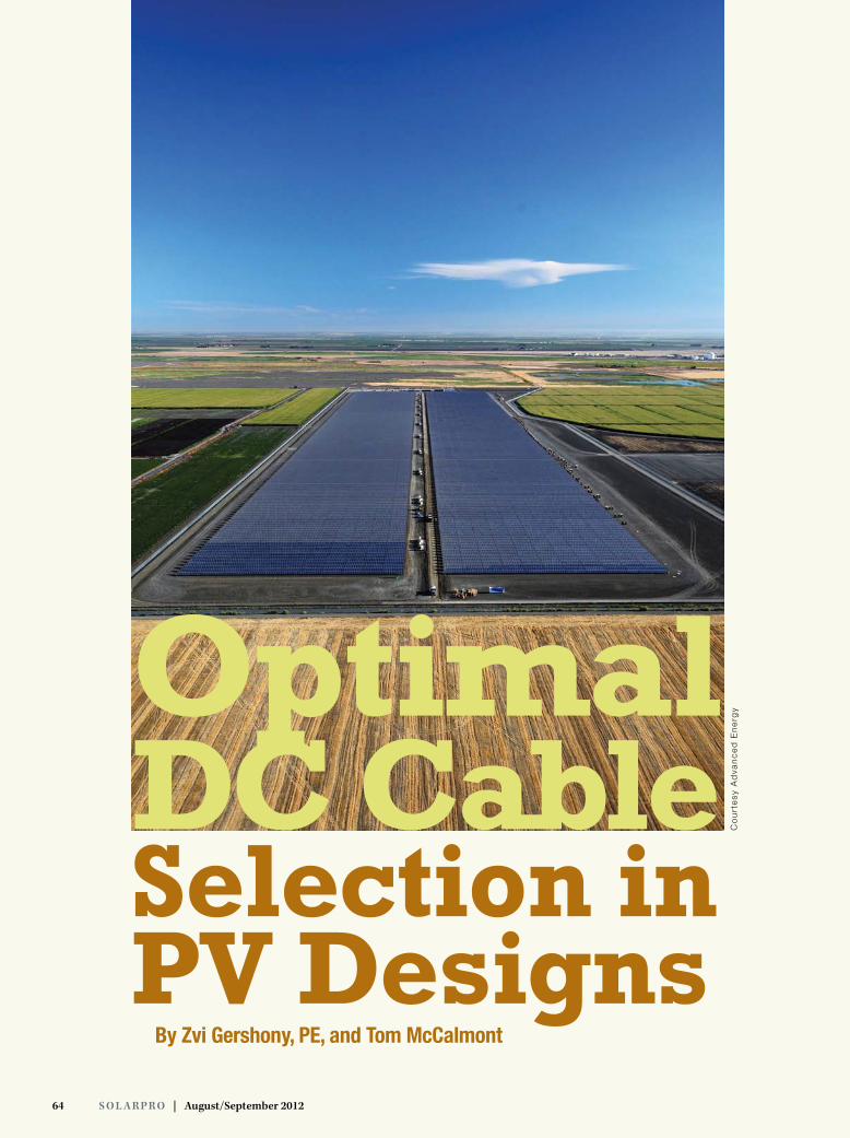
By Zvi Gershony, PE, and Tom McCalmont

Optimal DC Cable Selection in PV Designs

Co

urt

esy

Ad

van

ce

d E

ne

rgy

solarprofessional.com | S o l a r Pr o 65

PV designers spend a good deal of time assessing the optimal size of dc con-ductors, such as those that run from combiner boxes in a large array field to the location of the inverter. If these

conductors are specified too small, power losses erode a mean-ingful percentage of the potential solar energy harvest. If the conductors are specified too large, the cost of the conductors themselves becomes a meaningful proportion of overall system costs, driving up the levelized cost of energy. Neither situation is acceptable, yet there has been little quantitative analysis to determine optimal cable size.

In our engineering business designing large solar power plants, we frequently wrestle with this problem. We have mod-eled and analyzed it with the goal of optimizing the size, and therefore the cost, of these conductors for our customers. This article presents some of the surprising conclusions we have found through this analysis, which will help solar contractors determine optimal conductor sizing in terms of cost and trans-mission losses between the array and inverters.

Solar inverters are designed to operate within a wide range of dc input voltages to accommodate varying solar radiation levels. Determining voltage losses in the cables that deliver the solar power to inverters has traditionally been done via rules of thumb. For example, it is common practice in the electrical design industry to allow no more than a 5% voltage drop in cables. Such a limit is justified when designing commercial electrical systems for traditional industrial loads, such as motors, computer centers and lighting, which could be affected by voltages lower than nominal. Solar inverters, however, can operate flawlessly at lower dc input voltages—so long as they are within the operating voltage input window of the inverter. Therefore, if there were no other considerations, solar systems could be designed with greater voltage drops than 5% on the dc cables.

However, for economic reasons stemming from previously high module costs and high projected energy rates, designers have historically strived to minimize power losses on the dc con-ductors as much as possible by increasing the conductor size and cross-sectional area and, hence, the conductor cost. Many designers minimize losses on these conductors by designing for as little as 1.5% voltage drop as a standard for losses.

In this article, we suggest a method for optimally selecting the size of solar dc conductors considering only the solar irra-diation at the site, cable cost, utility tariff rates and financial factors. If math is not your passion, we present our key findings here in the text and tell you where to skip ahead when we get to the equations.

Cable Cost ModelThe cost model for installed dc conductors in a solar field con-sists of three separate elements:

1. D = costs that are proportional to the conductor cross-sectional area, such as the capital cost of the cable itself and the labor required to install it.

2. E = costs that are inversely proportional to the conductor cross-sectional area, such as energy losses due to resistance.

3. F = constant costs that are relatively unrelated to con-ductor cross-sectional area, such as the cost of trenching and conduits.

To simplify the model, we have assumed that a small variation in fixed costs, such as a slightly wider trench or a slightly larger conduit to accommodate larger conductors with respect to a reference conductor size, has a negligible impact on overall costs compared to the cost of the conduc-tors themselves. In other words, conduit and trenching costs do not change much, even if the required conductors increase or decrease a wire size or two.

In addition, as a model simplification, we assume that conductor cost is roughly proportional to the conductor’s cross-sectional area since conductor material (copper or alu-minum) is the dominant cost factor. This approximation is adequate if we assume that the optimal wire size is within a size or two of a wire size at a reference cross-sectional area for ampacity.

Ampacity Requirements The lower limit for required dc conductor size is derived from ampacity considerations. This is the minimum acceptable con-ductor size when applying ampacity calculations required by the National Electrical Code. We use this as our lower limit since in the design of large solar arrays, the conductor size derived based on required NEC ampacity considerations alone usually results in excessive voltage drops due to resistance, and the conductors must be upsized.

In this article, we assign the subscript A to all values result-ing from ampacity calculations. For instance, where S is used to indicate a conductor of a particular cross-sectional area, SA indicates the cross-sectional area of the minimally sized cable that has been selected to satisfy ampacity requirements.

Knowing the conductor cost structure of a minimally sized cable SA , the conductor cost at cross-sectional area S may be represented by the three cost elements DA , EA and FA as in Equa-tion 1:

where the conductor cost consists of capital cost, installa-tion labor, energy losses and fixed costs during the useful life of the cable.

It is clear from Equation 1 that as S approaches infinity, the first term dominates and Costconductor becomes very large. It is also clear that as S approaches zero, the second term dominates and Costconductor again grows very large. In other words, Equation 1 represents a bathtub curve, and we can conclude that between the two extremes there must be a minimum point between zero and very large. This point cor-responds to the ideal cable’s minimum cost and is the object of our pursuit.

Costconductor = DA + EA + FA 1

Costconductor' = DA − 2

= 3

DA = (U + W) × l × n 4

LA = × RA × n 5

K = 6

RA = ρ 7

LA = 8

EA = LA × T × γ25 9

EA = 10

= 11

Tc = 12

= 13

S = SA × 14

SSA

SA

S

SSA

EA

( )2

SSA( ) EA

DA

∑ h = 1

h = 8760 I h 2

lSA

K × Imp × 8760 × ρ × l × nSA × 1000

2

K × Imp × 8760 × ρ × l × n × T × γ25

SA × 1000

2

SSA

K × Imp × 8760 × ρ × T × γ25

SA × 1000 × (U + W)

2

SA × (U + W)K × Imp

× 8.76 × ρ × γ252

SSA

TTc

∑h = 1h = 8760

I mp 2 × 8760

I h 2

TTc

66 S o l a r Pr o | august/September 2012

Our Pursuit and Interesting Result Number One Rearranging the terms of Equation 1 and calculating the cable cost first derivative using S ÷ SA as the argument, we obtain Equation 2:

Since our pursuit is for the lowest cost cable that meets the requirements of both ampacity and voltage loss, we can substitute zero (the ideal minimum) for the first derivative, Costconductor', and then solve for the ratio of S to SA, which assures the minimum conductor cost:

This leads to our first interesting and somewhat surprising result: The selection of an optimally sized conductor does not require any knowledge of the constant cost factor, FA. In other words, the costs of trenches and conduits are not relevant to the selection of optimally sized conductors.

Note that the derivative of Equation 3 reflects the minimum conductor cost function, regardless of the ampacity require-ment. In the case where S ÷ SA <1, the minimum acceptable conductor size must continue to be SA since that is the mini-mum size required for ampacity. In that instance, we consider below whether a designer needs to increase the conductor size to reduce voltage losses. In the case where S ÷ SA >1, we develop a procedure for selecting the optimally sized conductor.

Calculating Proportional and Inversely Proportional Costs

Equation 3 tells us that to calculate S, the optimal cross- sectional area of our cable, we need to know the costs that are proportional and inversely proportional to the conductor cross-sectional area. Understanding the mathematics involved is not critical to our conclusions, so if you wish, you may safely skip ahead to the next section.

The costs DA that are proportional to conductor area may be expressed as:

where U is the unit cost of the conductor itself in dollars per meter ($/m), W is the labor (burdened wages) cost to install the conductor in dollars per meter ($/m), l is the point-to-point length of the conductors in meters (m), and n is the number of current-carrying conductors in a particular run.

The costs EA that are inversely proportional to conductor area are a function of energy losses related to resistance. The

smaller the conductor—and hence the less it costs—the greater the voltage losses due to resistance.

In a typical commercial installation such as a factory, electrical conductors for lighting or motors are designed to carry the designated current for 24 hours a day, year round. In a solar installation, however, the current carried by con-ductors from the combiner boxes varies from zero to Imp with the intensity of the sun throughout the day. Because of this difference, solar conductors are underutilized from a finan-cial investment viewpoint because they must be large enough to handle the highest current even while they are frequently idling throughout the day, carrying much lower currents.

The i2r losses LA in each run of n conductors in a solar field may be expressed in watt-hours per year as the sum of the losses for each of the 8,760 hours of solar generation in a year times the number of conductors:

where Ih is the current I in amperes during hour h, and RA is the conductor resistance in ohms. We can forecast the hourly current for a particular solar field based on the equipment being used and site conditions using a software program such as PVSyst.

Next, to evaluate this conductor’s economic utilization, we can define the shape factor K for the current I as follows:

This equation expresses the cable’s utilization from an eco-nomic viewpoint as a ratio of the current produced during each hour of generation versus the maximum power current if that were to be carried by the conductor every hour of the year. As Equation 6 shows, only site data and the Imp of the installed PV modules are required to calculate the shape factor.

Finally, the resistance of the cable in ohms can be expressed as:

where ρ is the specific resistance of the conductor measured in ohm-square millimeter per meter (Ω-mm2/m), and l is the length of the conductors in meters.

The value of ρ depends on whether the conductor is cop-per or aluminum. For copper at 75°C, the value of ρ is approximately 0.0222, and for aluminum, the value of ρ is approximately 0.0352. ρ is not a constant value. It depends on conductor temperature, which in turn depends on the cur-rent being carried and on-site conditions. However, since the change in ρ is small during normal conductor operation, we have assumed an average ρ that is constant. C o n t i n u E d o n pA g E 6 8



= 3

DA = (U + W) × l × n 4

LA = × RA × n 5

K = 6

RA = ρ 7

LA = 8

EA = LA × T × γ25 9

EA = 10

= 11

Tc = 12

= 13

S = SA × 14

SSA

SA

S

SSA

EA

( )2

SSA( ) EA

DA

∑ h = 1

h = 8760 I h 2

lSA

K × Imp × 8760 × ρ × l × nSA × 1000

2

K × Imp × 8760 × ρ × l × n × T × γ25

SA × 1000

2

SSA

K × Imp × 8760 × ρ × T × γ25

SA × 1000 × (U + W)

2


× 8.76 × ρ × γ252

SSA

TTc

∑h = 1h = 8760

I mp 2 × 8760

I h 2

TTc



= 3

DA = (U + W) × l × n 4

LA = × RA × n 5

K = 6

RA = ρ 7

LA = 8

EA = LA × T × γ25 9

EA = 10

= 11

Tc = 12

= 13

S = SA × 14

SSA

SA

S

SSA

EA

( )2

SSA( ) EA

DA

∑ h = 1

h = 8760 I h 2

lSA

K × Imp × 8760 × ρ × l × nSA × 1000

2

K × Imp × 8760 × ρ × l × n × T × γ25

SA × 1000

2

SSA

K × Imp × 8760 × ρ × T × γ25

SA × 1000 × (U + W)

2


× 8.76 × ρ × γ252

SSA

TTc

∑h = 1h = 8760

I mp 2 × 8760

I h 2

TTc



= 3

DA = (U + W) × l × n 4

LA = × RA × n 5

K = 6

RA = ρ 7

LA = 8

EA = LA × T × γ25 9

EA = 10

= 11

Tc = 12

= 13

S = SA × 14

SSA

SA

S

SSA

EA

( )2

SSA( ) EA

DA

∑ h = 1

h = 8760 I h 2

lSA

K × Imp × 8760 × ρ × l × nSA × 1000

2

K × Imp × 8760 × ρ × l × n × T × γ25

SA × 1000

2

SSA

K × Imp × 8760 × ρ × T × γ25

SA × 1000 × (U + W)

2


× 8.76 × ρ × γ252

SSA

TTc

∑h = 1h = 8760

I mp 2 × 8760

I h 2

TTc



= 3

DA = (U + W) × l × n 4

LA = × RA × n 5

K = 6

RA = ρ 7

LA = 8

EA = LA × T × γ25 9

EA = 10

= 11

Tc = 12

= 13

S = SA × 14

SSA

SA

S

SSA

EA

( )2

SSA( ) EA

DA

∑ h = 1

h = 8760 I h 2

lSA

K × Imp × 8760 × ρ × l × nSA × 1000

2

K × Imp × 8760 × ρ × l × n × T × γ25

SA × 1000

2

SSA

K × Imp × 8760 × ρ × T × γ25

SA × 1000 × (U + W)

2


× 8.76 × ρ × γ252

SSA

TTc

∑h = 1h = 8760

I mp 2 × 8760

I h 2

TTc



= 3

DA = (U + W) × l × n 4

LA = × RA × n 5

K = 6

RA = ρ 7

LA = 8

EA = LA × T × γ25 9

EA = 10

= 11

Tc = 12

= 13

S = SA × 14

SSA

SA

S

SSA

EA

( )2

SSA( ) EA

DA

∑ h = 1

h = 8760 I h 2

lSA

K × Imp × 8760 × ρ × l × nSA × 1000

2

K × Imp × 8760 × ρ × l × n × T × γ25

SA × 1000

2

SSA

K × Imp × 8760 × ρ × T × γ25

SA × 1000 × (U + W)

2


× 8.76 × ρ × γ252

SSA

TTc

∑h = 1h = 8760

I mp 2 × 8760

I h 2

TTc



= 3

DA = (U + W) × l × n 4

LA = × RA × n 5

K = 6

RA = ρ 7

LA = 8

EA = LA × T × γ25 9

EA = 10

= 11

Tc = 12

= 13

S = SA × 14

SSA

SA

S

SSA

EA

( )2

SSA( ) EA

DA

∑ h = 1

h = 8760 I h 2

lSA

K × Imp × 8760 × ρ × l × nSA × 1000

2

K × Imp × 8760 × ρ × l × n × T × γ25

SA × 1000

2

SSA

K × Imp × 8760 × ρ × T × γ25

SA × 1000 × (U + W)

2


× 8.76 × ρ × γ252

SSA

TTc

∑h = 1h = 8760

I mp 2 × 8760

I h 2

TTc

DC Cable Selection


Now, putting all three of the preceding equations together, we can express the annual losses for a particular run of conduc-tors as:

where a factor of 1,000 was added to express the result in kilowatt-hours per year.

The losses in Equation 8 recur every year until the end of the cable’s useful life. For solar power plants, we estimate that time frame at 25 years. If we assume that the utility buys the solar power at a tariff of T dollars per kilowatt-hour, then the annual economic loss in dollars over the life of the plant due to the use of this run of conductors can be expressed as LA × T.

This cost must be adjusted for inflation and expressed in terms of present value for the 25-year life of the plant. Calcu-lating the present value of a 25-year, $1 annuity, adjusted for inflation (see γ25 Calculations, p. 72), we express this as factor γ25, which, when multiplied by the economic loss in the first year, yields the total cost for use of this conductor over the expected life of the power plant:

Finally, substituting Equation 8 into Equation 9, we arrive at an expression for the costs that are inversely proportional to conductor area:

In summary, Equations 4 and 10 provide expressions for the costs of using a particular cable in a solar plant that are pro-portional and inversely proportional to the conductor cross-sectional area.

Interesting Result Number TwoThe fun part now is seeing the results that fall out of the preceding analysis. Equations 4 and 10 allow us to express the proportional and inversely proportional costs of a par-ticular cable, but those results can be simplified when com-bined in Equation 3 to solve for our optimally sized cable S of ideal cost:



= 3

DA = (U + W) × l × n 4

LA = × RA × n 5

K = 6

RA = ρ 7

LA = 8

EA = LA × T × γ25 9

EA = 10

= 11

Tc = 12

= 13

S = SA × 14

SSA

SA

S

SSA

EA

( )2

SSA( ) EA

DA

∑ h = 1

h = 8760 I h 2

lSA

K × Imp × 8760 × ρ × l × nSA × 1000

2

K × Imp × 8760 × ρ × l × n × T × γ25

SA × 1000

2

SSA

K × Imp × 8760 × ρ × T × γ25

SA × 1000 × (U + W)

2


× 8.76 × ρ × γ252

SSA

TTc

∑h = 1h = 8760

I mp 2 × 8760

I h 2

TTc



= 3

DA = (U + W) × l × n 4

LA = × RA × n 5

K = 6

RA = ρ 7

LA = 8

EA = LA × T × γ25 9

EA = 10

= 11

Tc = 12

= 13

S = SA × 14

SSA

SA

S

SSA

EA

( )2

SSA( ) EA

DA

∑ h = 1

h = 8760 I h 2

lSA

K × Imp × 8760 × ρ × l × nSA × 1000

2

K × Imp × 8760 × ρ × l × n × T × γ25

SA × 1000

2

SSA

K × Imp × 8760 × ρ × T × γ25

SA × 1000 × (U + W)

2


× 8.76 × ρ × γ252

SSA

TTc

∑h = 1h = 8760

I mp 2 × 8760

I h 2

TTc



= 3

DA = (U + W) × l × n 4

LA = × RA × n 5

K = 6

RA = ρ 7

LA = 8

EA = LA × T × γ25 9

EA = 10

= 11

Tc = 12

= 13

S = SA × 14

SSA

SA

S

SSA

EA

( )2

SSA( ) EA

DA

∑ h = 1

h = 8760 I h 2

lSA

K × Imp × 8760 × ρ × l × nSA × 1000

2

K × Imp × 8760 × ρ × l × n × T × γ25

SA × 1000

2

SSA

K × Imp × 8760 × ρ × T × γ25

SA × 1000 × (U + W)

2


× 8.76 × ρ × γ252

SSA

TTc

∑h = 1h = 8760

I mp 2 × 8760

I h 2

TTc

DC Cable Selection


Equation 11 demonstrates surprising result number two from our analysis: The optimal cross-sectional area and hence the cost of a particular cable run is independent of both cable length and the number of current-carrying conductors; those terms have fallen out of the equation. A fascinating corollary of this result is that since cable length is not a factor in determining optimal conductor size, volt-age drop, which is a function of conductor length, does not affect optimal conductor size either.

Critical Utility Tariff First, analyze Equation 11 for the case where S ≥ SA, when the optimally sized conductor is greater than the minimum size required to meet ampacity requirements. (When S < SA, the size of the conductor will be smaller than the minimum required to satisfy conductor ampacity requirements. In that case, SA must be selected as the optimal conductor size.)

A special case of interest is when S = SA, since this is when the optimal conductor cross-sectional area equals the

minimum cross-sectional area required for ampacity. There-fore, substituting the value 1 for S ÷ SA in Equation 11 and solving for T, we get:

expressed in dollars per kilowatt-hour ($/kWh). Note that the utility tariff T in Equation 12 has been designated as Tc to define it as the critical utility tariff at which S = SA, or in other words, the utility tariff that would be required for the optimally sized con-ductor on a particular run to be the same size as that required to meet ampacity requirements.

Optimum-Cost Cable and Interesting Result Number Three

For most solar power plants, T will not be equal to Tc , since the optimally sized conductor must be greater than the minimum size required for ampacity. When the local utility tariff T > Tc , we can substitute Tc from Equation 12 into Equation 11, which simplifies to:



= 3

DA = (U + W) × l × n 4

LA = × RA × n 5

K = 6

RA = ρ 7

LA = 8

EA = LA × T × γ25 9

EA = 10

= 11

Tc = 12

= 13

S = SA × 14

SSA

SA

S

SSA

EA

( )2

SSA( ) EA

DA

∑ h = 1

h = 8760 I h 2

lSA

K × Imp × 8760 × ρ × l × nSA × 1000

2

K × Imp × 8760 × ρ × l × n × T × γ25

SA × 1000

2

SSA

K × Imp × 8760 × ρ × T × γ25

SA × 1000 × (U + W)

2


× 8.76 × ρ × γ252

SSA

TTc

∑h = 1h = 8760

I mp 2 × 8760

I h 2

TTc



= 3

DA = (U + W) × l × n 4

LA = × RA × n 5

K = 6

RA = ρ 7

LA = 8

EA = LA × T × γ25 9

EA = 10

= 11

Tc = 12

= 13

S = SA × 14

SSA

SA

S

SSA

EA

( )2

SSA( ) EA

DA

∑ h = 1

h = 8760 I h 2

lSA

K × Imp × 8760 × ρ × l × nSA × 1000

2

K × Imp × 8760 × ρ × l × n × T × γ25

SA × 1000

2

SSA

K × Imp × 8760 × ρ × T × γ25

SA × 1000 × (U + W)

2


× 8.76 × ρ × γ252

SSA

TTc

∑h = 1h = 8760

I mp 2 × 8760

I h 2

TTc


where Tc was calculated as above, as the tariff at which S = SA . Rearranging Equation 13 to solve for S, the optimal conductor cross-sectional area, we get:

Equation 14 demonstrates our interesting result number three: An optimally sized conductor for a particular run in a solar power plant depends only on the local utility’s tariff paid for delivered solar energy as a function of the critical tariff rate at which S = SA. In other words, the cross-sectional area S of the optimally sized conductor to be used is expressed as a function of only SA, the conductor size required for ampac-ity; the local utility tariff T; and the critical utility tariff to Tc , which we can calculate.

It is also clear from Equation 14 that a special case is when T > Tc , as this corresponds to situations in which the optimally sized conductor S > SA , the conductor size for ampacity. In the case when T < Tc , S cannot be less than SA since the minimum acceptable conductor size must be SA, as determined by ampacity requirements.

Bringing It All TogetherAlthough the derivation was complex, the result is simple: Using a few well-known or easily determined parameters, you can follow a simple procedure to find the critical tariff Tc and from that derive the optimal conductor size. To calculate Tc , you need the following inputs:

• Minimum conductor size SA as derived from ampacity calculations,• Unit cost U for the cable selected and the labor cost W associated with its installation,• Solar insolation at the particular site, to determine K factor,• Solar module selected, to determine Imp, • Conductor material (copper or aluminum), to determine ρ, and• Expected inflation and discount rates for the next 25 years, to determine γ25.

Once you have calculated Tc and SA, you need to know only the local utility’s tariff, T, paid for delivered solar energy to calculate the optimal cross-sectional conductor size, S, using Equation 14. The metric result of that calculation should then be converted to a conductor size in kcmil for US installations.

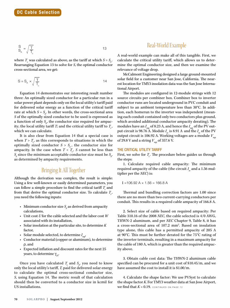
Real-World ExampleA real-world example can make all of this tangible. First, we calculate the critical utility tariff, which allows us to deter-mine the optimal conductor size, and then we examine the relevance of voltage drop.

McCalmont Engineering designed a large ground-mounted solar field for a customer near San Jose, California. The near-est location for TMY3 insolation data was the San Jose Interna-tional Airport.

The modules are configured in 12-module strings with 12 source circuits per combiner box. Combiner box to inverter conductor runs are located underground in PVC conduit and subject to an ambient temperature less than 30°C. In addi-tion, each homerun to the inverter was independent (mean-ing each conduit contained only two conductors plus ground, which avoided additional conductor ampacity derating). The modules have an Imp of 8.23 A, and hence the Imp of the PV out-put circuit is 98.76 A. Module Isc is 8.91 A and the Isc of the PV output circuit is 106.92 A. Working voltages are a module Vmp of 29.8 V and a string Vmp of 357.6 V.

THE CRITICAL UTILITY TARIFFFirst, we solve for Tc . The procedure below guides us through the steps:

1. Calculate required cable ampacity: The minimum required ampacity of the cable (the circuit Isc and a 1.56 mul-tiplier per the NEC) is:

I =106.92 A × 1.56 = 166.8 A

Thermal and bundling correction factors are 1.00 since there are no more than two current-carrying conductors per conduit. This results in a required cable ampacity of 166.8 A.

2. Select size of cable based on required ampacity: Per Table 310.16 of the 2008 NEC, the cable selected is 4/0 AWG, THWN-2 aluminum, and per NEC Chapter 9, Table 8, it has a cross-sectional area of 107.2 mm2. Based on insulation type alone, this cable has a permitted ampacity of 205 A at 90°C. This must be further derated for the 75°C rating of the inverter terminals, resulting in a maximum ampacity for the cable of 180 A, which is greater than the required ampac-ity above.

3. Obtain cable cost data: The THWN-2 aluminum cable specified can be procured for a unit cost of $10.45/m, and we have assumed the cost to install it is $1.00/m.

4. Calculate the shape factor: We use PVSyst to calculate the shape factor K. For TMY3 weather data at San Jose Airport, we find that K = 0.19. C o n t i n u E d o n pA g E 7 2



= 3

DA = (U + W) × l × n 4

LA = × RA × n 5

K = 6

RA = ρ 7

LA = 8

EA = LA × T × γ25 9

EA = 10

= 11

Tc = 12

= 13

S = SA × 14

SSA

SA

S

SSA

EA

( )2

SSA( ) EA

DA

∑ h = 1

h = 8760 I h 2

lSA

K × Imp × 8760 × ρ × l × nSA × 1000

2

K × Imp × 8760 × ρ × l × n × T × γ25

SA × 1000

2

SSA

K × Imp × 8760 × ρ × T × γ25

SA × 1000 × (U + W)

2


× 8.76 × ρ × γ252

SSA

TTc

∑h = 1h = 8760

I mp 2 × 8760

I h 2

TTc

DC Cable Selection



= 3

DA = (U + W) × l × n 4

LA = × RA × n 5

K = 6

RA = ρ 7

LA = 8

EA = LA × T × γ25 9

EA = 10

= 11

Tc = 12

= 13

S = SA × 14

SSA

SA

S

SSA

EA

( )2

SSA( ) EA

DA

∑ h = 1

h = 8760 I h 2

lSA

K × Imp × 8760 × ρ × l × nSA × 1000

2

K × Imp × 8760 × ρ × l × n × T × γ25

SA × 1000

2

SSA

K × Imp × 8760 × ρ × T × γ25

SA × 1000 × (U + W)

2


× 8.76 × ρ × γ252

SSA

TTc

∑h = 1h = 8760

I mp 2 × 8760

I h 2

TTc


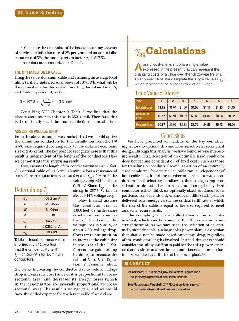
5. Calculate the time value of the losses: Assuming 25 years of service, an inflation rate of 2% per year and an annual dis-count rate of 5%, the annuity return factor γ25 is $17.53.

These data are summarized in Table 1.

THE OPTIMALLY SIZED CABLE Using the same aluminum cable and assuming an average local utility tariff for delivered solar power of 13¢/kWh, what will be the optimal size for this cable? Inserting the values for Tc , SA and T into Equation 14, we find:

Consulting NEC Chapter 9, Table 8, we find that the closest conductor to this size is 250-kcmil. Therefore, this is the optimally sized aluminum cable for this installation.

ASSESSING VOLTAGE DROP From the above example, we conclude that we should upsize the aluminum conductors for this installation from the 4/0 AWG size required for ampacity to the optimal economic size of 250-kcmil. The key point to recognize here is that this result is independent of the length of the conductors. Here we demonstrate this surprising result.

First, assume the length of the conductor run is just 50 feet. Our optimal cable of 250-kcmil aluminum has a resistance of 0.100 ohms per 1,000 feet, so at 50 feet and Imp of 98.76 A, the

voltage drop will be about 0.494 V. Since Vmp for the string is 357.6 V, this is about 0.14% voltage drop.

Now instead assume the conductor run is 1,000 feet. Using the same sized aluminum conduc-tor of 250-kcmil, the voltage loss is 9.88 V, or about 2.8% voltage drop. Contrary to our intuition to increase the cable size in the case of the 1,000-foot run, we gain nothing by doing so because the ratio of DA to EA in Equa-tion 3 remains about

the same. Increasing the conductor size to reduce voltage drop increases its cost (since cost is proportional to cross- sectional area) and decreases its energy losses (which in the denominator are inversely proportional to cross- sectional area). The result is no net gain, and we would have the added expense for the larger cable if we did so.

Conclusions We have presented an analysis of the key contribut-

ing factors to optimal dc conductor selection in solar plant design. Through this analysis, we have found several interest-ing results. First, selection of an optimally sized conductor does not require consideration of fixed costs, such as those for trenching or conduits. Second, selection of an optimally sized conductor for a particular cable run is independent of both cable length and the number of current-carrying con-ductors. Its fascinating corollary is that voltage drop con-siderations do not affect the selection of an optimally sized conductor either. Third, an optimally sized conductor for a particular run depends only on the local utility’s tariff paid for delivered solar energy versus the critical tariff rate at which the size of the cable is equal to the size required to meet ampacity requirements.

The example given here is illustrative of the principles involved, which can be complex. But the conclusions are straightforward. As we have seen, the selection of an opti-mally sized dc cable in a large solar power plant is a decision that should not be made based on voltage drop, regardless of the conductor lengths involved. Instead, designers should consider the utility tariff rates paid for the solar power gener-ated at the site to analyze the economic benefit of the conduc-tor size selected over the life of the power plant.

S = 107.2 x = 115.0 mm21311.3√

g C O N T A C T

Zvi Gershony, PE / Campbell, CA / McCalmont Engineering /

[email protected] / mccalmont.net

Tom McCalmont / Campbell, CA / McCalmont Engineering /

[email protected] / mccalmont.net

γ25Calculations

Time Value of Money

DC Cable Selection

Determining Tc

SA 107.2 mm2

U $10.45/m

W $1.00/m

K 0.19

Imp 98.76 A

ρ 0.0382 for Al

γ 25$17.53

Table 1 Inserting these values into Equation 12, we find that the critical utility tariff Tc = 11.3¢/kWh for aluminum conductors.

Year 1 2 3 4 5 6 7 8 9 10 11 12 13 14 15 16 17 18 19 20 21 22 23 24 25

Inflated Loss $1.02 $1.04 $1.06 $1.08 $1.10 $1.13 $1.15 $1.17 $1.20 $1.22 $1.24 $1.27 $1.29 $1.32 $1.35 $1.37 $1.40 $1.43 $1.46 $1.49 $1.52 $1.55 $1.58 $1.61 $1.64

Discounted Loss

$0.97 $0.94 $0.92 $0.89 $0.87 $0.84 $0.82 $0.79 $0.77 $0.75 $0.73 $0.71 $0.69 $0.67 $0.65 $0.63 $0.61 $0.59 $0.58 $0.56 $0.54 $0.53 $0.51 $0.50 $0.48

Present Value $0.97 $1.92 $2.83 $3.72 $4.59 $5.43 $6.24 $7.04 $7.81 $8.56 $9.28 $9.99 $10.68 $11.34 $11.99 $12.62 $13.23 $13.82 $14.40 $14.96 $15.50 $16.03 $16.54 $17.04 $17.53

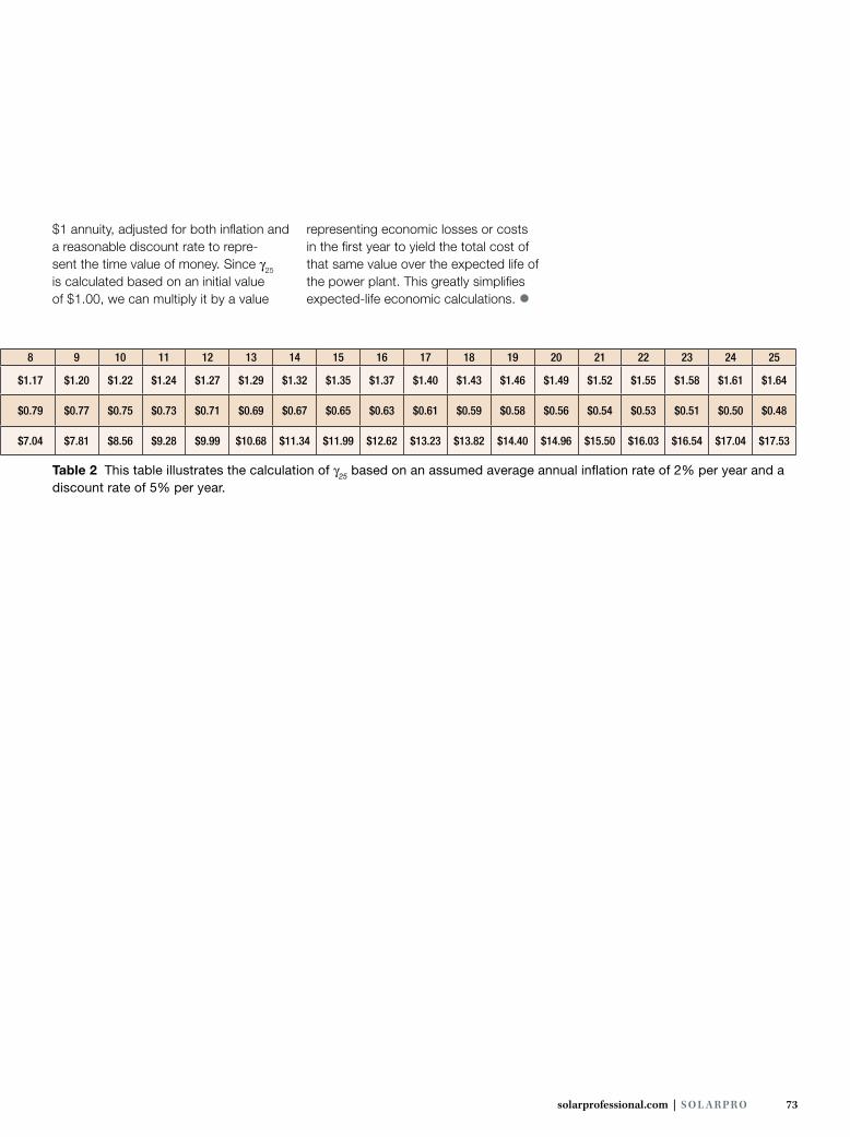
A useful cost-analysis tool is a single value expressed in the present that can represent the

changing costs of a value over the full 25-year life of a solar power plant. We designate this single value as γ25, which represents the present value of a 25-year,

http://www.mccalmont.net

http://www.mccalmont.net


Table 2 This table illustrates the calculation of γ25 based on an assumed average annual inflation rate of 2% per year and a discount rate of 5% per year.

Year 1 2 3 4 5 6 7 8 9 10 11 12 13 14 15 16 17 18 19 20 21 22 23 24 25

Inflated Loss $1.02 $1.04 $1.06 $1.08 $1.10 $1.13 $1.15 $1.17 $1.20 $1.22 $1.24 $1.27 $1.29 $1.32 $1.35 $1.37 $1.40 $1.43 $1.46 $1.49 $1.52 $1.55 $1.58 $1.61 $1.64

Discounted Loss

$0.97 $0.94 $0.92 $0.89 $0.87 $0.84 $0.82 $0.79 $0.77 $0.75 $0.73 $0.71 $0.69 $0.67 $0.65 $0.63 $0.61 $0.59 $0.58 $0.56 $0.54 $0.53 $0.51 $0.50 $0.48

Present Value $0.97 $1.92 $2.83 $3.72 $4.59 $5.43 $6.24 $7.04 $7.81 $8.56 $9.28 $9.99 $10.68 $11.34 $11.99 $12.62 $13.23 $13.82 $14.40 $14.96 $15.50 $16.03 $16.54 $17.04 $17.53

$1 annuity, adjusted for both inflation and a reasonable discount rate to repre-sent the time value of money. Since γ25 is calculated based on an initial value of $1.00, we can multiply it by a value

representing economic losses or costs in the first year to yield the total cost of that same value over the expected life of the power plant. this greatly simplifies expected-life economic calculations. {

Documents

Optimal DC Cable Courtesy Advanced Energy Selection …mccalmont.fatcow.com/...optimal-dc-cable-selection-in-pv-designs.pdf · DC Cable Selection in PV Designs Courtesy Advanced Energy