Optimal Need-Based Financial Aid∗

Sebastian FindeisenUniversity of Mannheim

Dominik SachsEuropean University Institute

July 4, 2017

Abstract

We study the optimal design of student financial aid as a function of parental income.We characterize the sufficient statistics of the policy problem in a general model. Fora simple model version, we derive mild conditions on primitives under which poorerstudents receive more aid even without distributional concerns. We quantitatively extendthis result to an empirical model of selection into college for the U.S. We allow forheterogeneity in parental transfers, returns to college, and other variables. Optimalfinancial aid is strongly declining in parental income also without distributional concerns.Equity and efficiency go hand in hand.

JEL-classification: H21, H23, I22, I24, I28

Keywords: Financial Aid, College Subsidies, Optimal Taxation, Inequality

∗Contact: findeisen@uni-mannheim.de, dominik.sachs@eui.eu. An earlier version of this paper was cir-culated under the title Designing Efficient College and Tax Policies. We thank Rüdiger Bachmann, FelixBierbrauer, Richard Blundell, Christian Bredemeier, Friedrich Breyer, David Card, Pedro Carneiro, JuanDolado, Alexander Gelber, Marcel Gerard, Emanuel Hansen, Nathaniel Hendren, Bas Jacobs, Leo Kaas,Marek Kapicka, Kory Kroft, Paul Klein, Tim Lee, Lance Lochner, Normann Lorenz, Thorsten Louis, AlexLudwig, Marti Mestieri, Nicola Pavoni, Michael Peters, Emmanuel Saez, Aleh Tsyvinski, Gianluca Violante,Matthew Weinzierl, Nicolas Werquin and seminar participants at seminar participants at Berkeley, Bocconi,Bonn (MPI & MEE), CEMFI, Dortmund, EIEF, EUI, Frankfurt, IFS/UCL, Louvain (CORE), Notre Dame,Lausanne, Queen’s, Salzburg, St. Gallen, Toronto, Toulouse, Uppsala, Warwick as well as conference partici-pants at CEPR Public Meeting 16, CESifo Public Sector Economics, IIPF, NBER SI Macro Public Finance,NORMAC, SEEK and the Taxation Theory Conference. Dominik Sachs’ research was partly funded by a post-doc fellowship of the Fritz-Thyssen Foundation and the Cologne Graduate School in Management, Economicsand Social Sciences.

1 Introduction

In all OECD countries, college students benefit from financial support (OECD, 2014). More-

over, with the goal of guaranteeing equality of opportunity, financial aid is typically need-based

and targeted specifically to students with low parental income. In the United States the largest

need-based program is the Pell Grant. Federal spending on this program exceeded $30 billion

in 2015 and has grown by over 80% during the last 10 years (College Board, 2015).

One justification for student financial aid in the policy debate is that the social returns

to college exceed the private returns because the government receives a share of the financial

returns through higher tax revenue (Carroll and Erkut, 2009; Baum et al., 2013). This lowers

the effective fiscal costs (i.e. net of tax revenue increases) of student financial aid.

The Congressional Budget Office (CBO), following a request by the Senate Committee

on the Budget, recently documented the growth in the fiscal costs of Pell Grant spending

(Alsalam, 2013). Dynamic scoring aspects are neglected in this report: the positive fiscal

effects through higher tax revenue in the future are not taken into account.1

In this paper, we study the optimal design of financial aid and show that considering

dynamic scoring aspects is crucial to assess the desirability of need-based programs like the

Pell Grant. The reduction of effective fiscal costs of student financial aid due to dynamic

fiscal effects varies along the parental income distribution. We show that the effective fiscal

costs are increasing in parental income and are therefore lowest for those children that are

targeted by the Pell Grant. The policy implication is that need-based financial aid is not only

desirable because it promotes intergenerational mobility and equality of opportunity. Need-

based financial aid is also desirable from an efficiency point of view because subsidizing college

education of children with weak parental background is cheaper for society than subsidizing

students from an "average" parental background. The usual equity-efficiency trade-off does

not apply for need-based financial aid.

To arrive there, we start with a general model without imposing restrictions on the under-

lying heterogeneity in the population and express the optimality conditions for financial aid

in terms of four sufficient statistics. The formula transparently highlights the key trade-offs

of the problem. At a given level of parental income, optimal financial aid decreases in the

share of inframarginal students, which captures the marginal costs. These costs are scaled

down by the marginal social welfare weights attached to these students. Optimal financial aid

increases in the share of marginal students2 and the fiscal externality per marginal student,

which jointly capture the marginal benefits of the subsidy. The fiscal externality is the change

of lifetime fiscal contributions causal to college attendance. For the optimality condition, the1Generally, the CBO does consider issues of dynamic scoring: https://www.cbo.gov/publication/

50919.2Those students that are at the margin of attending college with respect to financial aid.

1

specific reason why marginal students change their behavior due to a change in subsidies is

not important (e.g. borrowing constraints or preferences): the share of marginal students is a

sufficient statistic or policy elasticity (Chetty, 2009; Hendren, 2015).

Although this policy elasticity has been estimated frequently in the literature (e.g. by

Dynarski (2003) and Castleman and Long (2016)), it has – perhaps surprisingly – not yet been

exploited to study the optimal design of financial aid.3 These papers provide guidance about

the average value of this policy elasticity or about its value at a particular parental income

level. However, knowledge about how this policy elasticity varies along the parental income

distribution is missing. Further, policy elasticities are not deep parameters but might change

substantially as policy changes. The main approach of this paper is therefore a structural

model of selection into college that provides numbers for this policy elasticity along the parental

income distribution and for alternative policies. The mentioned quasi-experimental studies

provide an empirical moment that we target with our model.

As a first step, however, before studying this empirical model of selection into college, we

consider a simple theoretical setting for which we obtain closed form solutions for our sufficient

statistics. We reduce the complexity of the problem by focusing on (i) the role of parental

transfers and (ii) heterogeneity in the returns to college. We show under which conditions

low-parental-income students should receive more aid. As in the more general model, this

depends on the ratio of marginal students, which scale the fiscal benefits of financial aid,

to the fraction of inframarginal students, which the scale the fiscal costs. In this simple

setting, this ratio is pinned down by the hazard rate of the distribution of returns. If this

hazard rate is decreasing – which is true, for example, for the normal distribution – optimal

financial aid is progressive even in the absence of distributional concerns between students with

different parental background.4 This theoretical exercise provides a lot of intuition behind the

mechanisms that determine the optimal level of student financial aid along the parental income

distribution. However, it relies on some unrealistic assumptions, e.g., it abstracts from the fact

that parental income and ability of the children at age 18 are positively correlated (Carneiro

and Heckman, 2003; Altonji and Dunn, 1996). We do account for this correlation in our

structural model, however.

We estimate our structural model with data from the National Longitudinal Survey of

Youth 1979 and 1997, which contains information on parental income and ability determined

before college as measured by the Armed Forced Qualification Test Score (AFQT). Using

simple regressions, we estimate how parental income, AFQT and college education determine3A notable exception is Lawson (2016) who studies optimal tuition subsidies in a homogenous agent setting

and therefore disregards the question on how such policies should vary with parental income.4The model ignores three mechanisms which would lead to a a higher progressiveness. First, borrowing

constraints for lower income households naturally would give the government an incentive to provide liquiditywith financial aid. Second, a higher welfare weight placed on low-income students would give a redistributivegain. Third, utility costs of attending college which differ across income groups.

2

other variables of our model: the distribution from which individuals draw their wage (to cap-

ture returns to college), parental transfers (to capture the direct impact of parental income)

and financial aid receipt (to capture the current degree of need and merit based elements). An

additional crucial ingredient of the model is heterogeneity in the psychic costs of education

because monetary returns can only account for a small part of the observed college atten-

dance patterns (Heckman et al., 2006). We estimate the distribution of psychic costs through

maximum likelihood in a discrete choice model to fit college decisions in the data.

The model successfully replicates quasi-experimental studies: First, it is consistent with es-

timated elasticities of college attendance and graduation rates w.r.t. financial aid expansions

(Deming and Dynarski, 2009). Second, it is consistent with the causal impact of parental in-

come changes on college graduation rates (Hilger, 2016). Further, our model yields (marginal)

returns to college that are in line with the empirical literature (Card, 1999; Oreopoulos and

Petronijevic, 2013; Zimmerman, 2014).

We find that optimal financial aid policies are strongly progressive. In our preferred spec-

ification, the level of financial aid drops by more than 60% moving from the 5th percentile

of the parental income distribution to the 95th percentile. The strong progressivity is very

robust and holds for a broad range of different parameter choices: different tax functions,

welfare criteria, and assumptions on credit markets. In particular, we find that even for a

government purely interested in maximizing tax revenue, progressive financial aid is the best

policy. Second, our estimates suggest that targeted increases in financial aid for low-income

students, approximately between the 15th and 45th percentile of the parental income distribu-

tion, are self-financing by increases in future tax-revenue; this implies that targeted financial

aid expansions could be Pareto improving free-lunch policies. Both results point out that

financial aid policies for students are a rare case where there is no equity-efficiency trade-off:

education policies which lead to a cost-effective distribution of financial aid are also in line

with redistributive concerns and social mobility.

One may have expected that efficiency considerations would make a case against need-based

financial aid because of the positive correlation between returns to college and parental income.

This correlation is indeed positive in our empirical model and the fiscal externality of the

average marginal student with high parental income is much higher (up to a factor of 3) than

for the average marginal student with low parental income. However, this effect is dominated

by the fact that at higher parental income levels much more students are inframarginal.

Finally, we also allow the government to optimally set the Mirleesian tax schedule.5 The

optimal Utilitarian tax system has higher average tax rates than the current US tax schedule.5The main text contains the quantitive results for this exercise and the theoretical characterization is in

the appendix. Since college enrollment is modeled as a binary choice, our formal approach is similar to optimaltax papers with both, intensive and extensive margin, as in Saez (2002). This part is also related to otherrecent papers that study optimal (history-independent) income taxation with endogenous skills such as Bestand Kleven (2013) and Heathcote et al. (2016).

3

This has large implications for the average level of the education subsidy which is now twice

as high, compared to the case with the current US tax schedule. But the main result is also

obtained with an endogenous optimal tax schedule. The optimal financial aid system features

a negative dependence on parental income also if the income tax is optimally designed.

Our paper contributes to the existing literature in several ways. Stantcheva (2016) char-

acterizes optimal human capital policies in a very general dynamic model with continuous

education choices. The main differences with our approach are twofold. First, theoretically,

the education choice has to be discrete if one wants to study optimal financial aid policies

and, as we show, the optimality conditions are quite distinct from the continuous case and

different elasticities are required to characterize the optimum.6 Second, the extensive margin

education decision allows to incorporate a large degree of heterogeneity without making the

optimal policy problem intractable. This allows for a modeling approach close to the empirical,

structural literature.

Bovenberg and Jacobs (2005) consider a static model with a continuous education choice

and derive a ‘siamese twins’ result: they find that the optimal marginal education subsidy

should be as high as the optimal marginal income tax rate, which fully offsets the distor-

tions from the income tax on the human capital margin.7 Lawson (2016) uses a sufficient

statistic approach to characterize optimal uniform tuition subsidies for all college students.8

We contribute to this line of research by developing a new framework to analyze how edu-

cation policies should depend on parents’ resources9 and also trade-off merit-based concerns.

Our theoretical characterization of optimal financial aid (and tax policies) allows for a large

amount of heterogeneity, and we tightly connect our theory directly to the data by estimating

the relevant parameters ourselves. Finally, the paper is also related to many empirical papers,

from which we take the evidence to gauge the performance of the estimated model. Those

papers are discussed in detail in Section 4.

We progress as follows. In Section 2 we develop the general model and study optimal policies

in terms of sufficient statistics. In Section 3 we consider a simplified version of the model,

which allows to transparently study mild conditions on primitives implying that financial

aid is optimally decreasing in parental income. In Section 4 we describe our calibration6This resembles the different results in the optimal tax literature along the extensive versus the intensive

margin (Diamond, 1980; Saez, 2001, 2002).7Bohacek and Kapicka (2008) derive a similar result as in a dynamic deterministic environment. In

Findeisen and Sachs (2016), we focus on history-dependent policies and show how history-dependent laborwedges can be implemented with an income-contingent college loan system. Koeniger and Prat (2017) studyoptimal history-dependent human capital policies in a dynastic economy where education policies also dependon parental background. Stantcheva (2015) derives education and tax policies in a dynastic model with multi-dimensional heterogeneity, characterizing the relationship between education and bequest policies.

8Our work is also complementary to Abbott et al. (2016) and Krueger and Ludwig (2013, 2016) who studyeducation policies computationally in very rich overlapping-generation models.

9Gelber and Weinzierl (2016) study how tax policies should take into account that the ability of childrenis linked to parents’ resources and find that the optimal policy is more redistributive towards low incomefamilies.

4

and estimation approach and discuss the relationship to previous empirical work. Section 5

presents optimal financial aid policies and Section 6 considers the jointly optimal education

and tax policies. In Section 7 we discuss the robustness of our results with respect to college

dropout and general equilibrium effects on wages. Section 8 concludes.

2 Optimal Financial Aid Policies

In this section we characterize optimal financial aid policies for college students. We start by

stressing the need-based component of financial aid and derive optimal policies as a function

of parental income. Optimal policies will be a function of a set of estimable parameters. In

particular, the elasticity of college graduation rates w.r.t. changes in financial aid generosity,

the returns for marginal students, and the fraction of inframarginal students will be the key

forces driving the most important results. Subsequently, we also allow the government to

condition financial aid policies on other observables like academic merit or jointly on the

combination of parental income and academic merit.

In the model, individuals start life as high school graduates and decide whether to obtain

a college degree. If an individual decides against a college degree, she directly enters the

labor market. The decision to enroll in college will depend on a vector of characteristics X.

For example, potential students may be aware of their returns to college and these returns

are likely to be heterogeneous. It could also capture geographical origins, endurance or any

other aspect that influences the decision to study. In addition to the sources of heterogeneity

in X, parental income I can determine the college decision. We stress this dimension as an

extra parameter because of our strong focus on the need-based element of student financial

aid. Parental income I is associated with parental transfers during college. Parental transfers

matter for two reasons. First, parental transfers matter because of (potentially binding)

borrowing constraints. Second, parental transfers act as a price subsidy because parents make

transfers contingent on the educational decision.

The model also incorporates uncertainty about labor market outcomes. We focus on a

simple two period version of the model with an education period and a labor market period.

It is inconsequential for the interpretation of the optimal financial aid formulas, as they also

hold if taxable incomes and wages change over the life cycle.

2.1 Individual Problem

Individuals graduate from high-school and are characterized by a vector X ∈ χ and (perma-

nent) parental income I ∈ R+. A type (I,X) is also labeled by j. Individuals face a binary

choice at the beginning of the model: enrolling in college or not. We assume that life after

the college entry decision lasts T years, college takes Te years and individuals’ yearly discount

5

factor is β. Then we can think of βC1 =∑Te

t=1 βt−1 and βC2 =

∑Tt=Te+1 β

t−1. If a young

individual j enrolls, her expected lifetime utility is:

βC1UC(cCj ; I,X) + βC2

∫Ω

UW(cWjw, y

Wjw;w, I,X

)dGC(w|I,X).

UC(cCj ; I,X) denotes utility during the college years. It depends on consumption cCj during

those years, and level of consumption will depend on j = (I,X). For example higher parental

income is strongly associated with higher parental transfers during college. I and X can

also have a direct utility effect of attending college; for example empirical studies have found

a strong correlation between parents’ and children’s educational attainment, conditional on

parental income. This would be captured by the direct effect of X.

The wage w ∈ Ω is drawn from a conditional distribution function GC(w|I,X). X can

include, for example, a measure of ability, which leads to heterogeneous returns to college.

Empirical paper have stressed the importance of complementarity between ability measures

and college education, which can be flexibly captured by GC(w|I,X). Consumption and tax-

able income during the working life are cWjw and yWjw. They depend on the wage draw, as well as

the type from the previous period. We assume that the utility function UW(cWjw, y

Wjw;w, I,X

)is such that there are no income effects on labor supply. We discuss the relaxation of this

assumption in Section 7.

The problem of a college graduate with parental income I and vector X becomes:

V C(I,X;G(I), T (.)) = maxcCj ,c

Wjw,y

Wjw

βC1UC(cCj ; I,X) + βC2

∫Ω

UW(cWjw, y

Wjw;w, I,X

)dGC(w|I,X)

subject to

∀ w : cWjw = yWjw − T (yWjw)− (1 + r)L

and

cCj = trC(I) + G(I)− C + L,

and

L ≤ L.

where, as explained above, βC1 and βC2 capture discounting and the different length of periods

as described above. T (.) are taxes on earnings. trC(I) is the transfer function mapping

parental income into transfers received when going to college. Students can take loans L with

some interest r. Potentially, there may be an exogenous borrowing limit on loans taken out

given by L. The government runs a financial aid program G(I) which subsidizes college costs

based on financial needs. C represents the tuition cost of attending college.

6

Expected utility of a high-school graduate entering the labor market directly is:

βH∫

Ω

UH(cHjw, y

Hjw;w, I,X

)dGH(w|I,X),

where βH = βC1 +βC2 captures the length of the labor market period of high school graduates.

The wage realization is drawn from a different conditional distribution GH(w|I,X), but is

allowed to depend on attributes in X. Importantly, ability should be expected to influence

wages also for high-school graduates. The difference in GH(w|I,X) and GC(w|I,X) captures

returns to college. A natural assumption would be that the latter first-order stochastically

dominates the former. For our theoretical considerations, however, we do not need to impose

such an assumption. We will from now on refer to all individuals not attending college as

high-school graduates. The problem of a high-school graduate with parental income I and

vector X becomes:

V H(I,X;T (.)) = maxcHjw,y

Hjw

βH∫

Ω

UH(cHjw, y

Hjw;w, I,X

)dGH(w|I,X)

subject to

∀ w : cHjw = yHjw − T (yHjw) + trH(I).

So a high-school graduate solves a static problem under this formulation. Note that we also

allow for the possibility that high-school graduates receive financial support from their parents

trH(I). We observe positive transfers in the data also for working high-school graduates and

the majority of these transfers happen at the beginning of the working life.

Finally, each type (I,X) decides to attend college or not, comparing V C(I,X;G(I), T (.))

and V H(I,X;T (.)). We assume that the value functions are differentiable in policies.

2.2 Government Problem and Optimal Policies

We now characterize the optimal level of financial aid function G(I) for a given tax function.

We denote by F (I) the unconditional parental income distribution, by K(I,X) the joint

c.d.f. and by H(X|I) the conditional one; the densities are f(I), k(I,X) and h(X|I). The

government assigns Pareto weights k(I,X) = f(I)h(X|I) which are normalized to integrate

up to one.

Importantly, we assume that the government takes the income tax T (·) as given and the

optimal reform of G(I) has to be budget neutral. We consider this as the more policy relevant

exercise than considering also the optimal choice of T (·). Nevertheless, to complete the picture,

in Section 6, we consider the joint optimal design of financial aid G(I) and the tax-transfer

system T (·).

7

Taking the tax-transfer system as given, the problem of the government is:

maxG(I)

∫R+

∫χ

maxV C(I,X), V H(I,X)k(I,X)dIdX (1)

subject to the government budget constraint:

∫R+

∫χ

βC1G(I)1V Cj ≥V Hj k(I,X)dIdX =

∫Ω

∫R+

∫χ

βHT (yHjw)1V Cj <V Hj k(I,X)dIdXdGH(w|I,X)

+

∫Ω

∫R+

∫χ

βC2T (yWjw)1V Cj ≥V Hj k(I,X)dIdXdGC(w|I,X),

where 1V Cj <V Hj and 1V Cj ≥V Hj are indicator functions capturing the education choice for each

type j = (I,X). The budget constraint simply equates government spending on financial aid

to tax revenues. We label the multiplier on the budget constraint with ρ and assume, for

notational convenience, that the government discounts tax revenue at the same rate as the

agents discount utility.

Before we derive optimal education subsidies, we ease the upcoming notation a little bit

and define the share of college students at parental income level I as follows:

FC(I) =

∫χ

1V Cj ≥V Hj h(X|I)dX.

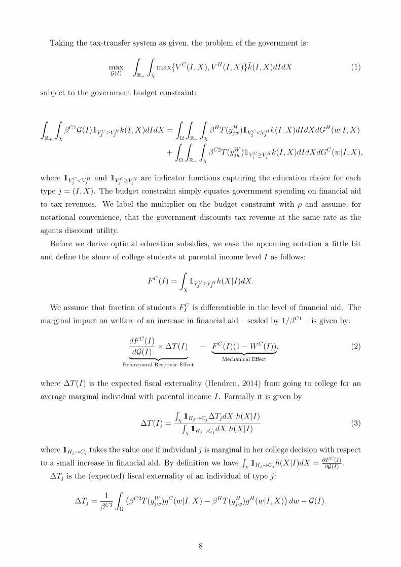
We assume that fraction of students FCI is differentiable in the level of financial aid. The

marginal impact on welfare of an increase in financial aid – scaled by 1/βC1 – is given by:

dFC(I)

dG(I)×∆T (I)︸ ︷︷ ︸

Behavioural Response Effect

− FC(I)(1−WC(I))︸ ︷︷ ︸Mechanical Effect

, (2)

where ∆T (I) is the expected fiscal externality (Hendren, 2014) from going to college for an

average marginal individual with parental income I. Formally it is given by

∆T (I) =

∫χ

11Hj→Cj∆TjdX h(X|I)∫χ

11Hj→CjdX h(X|I)(3)

where 11Hj→Cj takes the value one if individual j is marginal in her college decision with respect

to a small increase in financial aid. By definition we have∫χ

11Hj→Cjh(X|I)dX = ∂FC(I)∂G(I)

.

∆Tj is the (expected) fiscal externality of an individual of type j:

∆Tj =1

βC1

∫Ω

(βC2T (yWjw)gC(w|I,X)− βHT (yHjw)gH(w|I,X)

)dw − G(I).

8

Generally one should expect ∆Tj to be positive if returns to college (captured by the difference

in the wage distributions GH(w|I,X) and GC(w|I,X)) are sufficiently large. If the increase

in annual earnings due to college education is rather low, ∆Tj could be negative (i) because

of the subsidies G(I) paid and (ii) because college graduates enter the labor market later and

work fewer years (both captured by βH < βC2).

The behavioral response effect in (2) captures exactly these fiscal benefits of more financial

aid. The reform will trigger enrollment from a certain set of students with parental income

level I, those who were at the margin of enrolling before the reform. We denote these studentsdFC(I)dG(I)

as marginal students. They were just indifferent between going to college or not, so

their change in decision has no first-order effect on welfare. However, they contribute to public

funds which is captured by the fiscal externality ∆T (I).

The second term in (2) captures the mechanical aspect of the reform: for all inframarginal

students FC(I) at the parental income level in question, the government has to spend one

more dollar. The marginal costs are scaled down by the welfare weights on students

WC(I) =f(I)

f(I)

∫χ1V C≥V HU

Cc (cCj ; I,X)h(I|X)dX,

ρ

where UCc is the marginal utility of consumption and ρ is the marginal value of public funds –

thus, WC(I) is the money-metric marginal social welfare weight (Saez and Stantcheva, 2016).

Summing up, to understand the welfare effects of an increase in financial aid G(I) one

needs to know four sufficient statistics: (i) the share of marginal students, (ii) the average

fiscal externality per marginal student, (iii) the share of infra-marginal students and (iv) the

social marginal welfare weight the students.10

Multiplying (2) by G(I) and setting to zero yields a formula for the optimal level of financial

aid at parental income I:

G(I) =η(I)∆T (I)

FC(I)(1−WC(I))(4)

where η(I) is a local semi elasticity of college enrollment rates: the percentage point change

in the share of students in parental income group I in terms of a percentage change in G(I).

Formally it is given by η(I) = dFC(I)dG(I)/G(I)

.

The formula for optimal financial aid (4) has a very intuitive interpretation. Optimal

financial aid is increasing in the effectiveness of increasing college attendance measured by

η(I); such behavioral responses have been estimated in the literature exploiting financial aid10Note that if the utility function UW

(cWjw, y

Wjw;w, I,X

)would not satisfy the no income effect assumption,

there would be an additional effect. If individuals are not borrowing constraint during college, an increase infinancial aid will decrease their borrowing. If leisure is a normal good, this would then imply less labor supplyand therefore a decrease in tax payment. We discuss the implications of this in Section 7.

9

reforms, see the discussion in Section 4.3. This behavioral effect is a policy elasticity as

discussed in Hendren (2015). This effect is weighted by the fiscal externality created, i.e.

the increase in tax payments. Intuitively, the size of the fiscal externality will depend on

the returns to college for marginal students, another parameter which has been estimated

in different contexts in prior work. Optimal financial aid is decreasing in the number of

inframarginal students, capturing the cost of financial aid, and increasing in the value placed

on college students’ welfare.

The formula is a sufficient statistic formula, providing intuition for the main trade-offs

underlying the design of financial aid. It is valid without taking a stand on the functioning

of credit markets for students, the riskiness of education decisions or the exact modeling

how parental transfers are influenced by parental income. Changes in those factors would of

course influence the values of the sufficient statistics. For example, a tightening of borrowing

constraints should increase the sensitivity of enrollment especially for low income students.

Notice that the essence of the main trade-offs are unchanged if taxable incomes change

over the life-cycle. This affects the calculation of the term Tj which then reflects the differ-

ence in discounted present values of yearly tax payments over the life-cycle. Additionally, if

wages change stochastically over the life-cycle, the fiscal externality still reflects differences in

expected tax payments for the group of marginal students.

Besides studying the optimal level, our approach allows to answer a related but different

question: to what extent could small reforms to the current US financial aid be self-financing

through higher future tax-revenue? We consider this as an interesting complementary question

for at least two reasons. First, it may be easier to implement small reforms to the existing

current federal financial aid system. Second, it points out whether there are potential Pareto

improving free-lunch policy reforms on the table which are independent of the underlying

welfare function.

Setting WC(I) = 0 to focus on fiscal magnitudes, we can rewrite (2) and obtain an expres-

sion for the fiscal return R(I) of increasing financial aid:

R(I) =

∂FC(I)∂G(I)

∆T (I)

FC(I)− 1 (5)

This expression can be interpreted as the rate of return on one dollar invested in additional

college subsidies at income level I. If it takes the value .2, it says that the government gets

$1.20 in additional tax revenue for one marginal dollar invested into college subsidies. If it

is -.5, it implies that the government gets 50 Cents back for each dollar invested – increasing

subsidies by one dollar costs the government only 50 Cents per dollar spent. Therefore, another

way of interpreting (5) is to say that the effective costs of providing one more dollar to students

of parental income level I is equal to −R(I) dollar. Whenever enrollment is responsive (i.e.

10

∂FC(I)∂G(I)

> 0) and education is sufficiently beneficial such that ∆T (I) > 0, effective marginal

costs are below one dollar.

2.3 Merit-Based Policies

Our approach is more general and can be extended to condition financial aid policies on other

observables like academic merit or jointly on the combination of parental income and academic

merit. In fact, in our empirical application we will allow the government to also target financial

aid policies on a signal of academic ability. Suppose the government can observe such a signal

of academic ability like the SAT score. We take that factor out of the vector X and label it

θ. For notational simplicity, we will still denote the vector without θ by X; in this case X

includes all factors influencing the college decision except for parental income and the measure

of academic ability. Suppose we are interested in deriving the optimal policy schedule which

conditions on need- and merit-based components jointly. Formally, the government maximizes

over G(I, θ). The derivation of the optimal financial aid policy schedule is analogous to the

derivation of G(I) and yields:

G(I, θ) =η(I, θ)∆T (I, θ)

FC(I, θ)(1−WC(I, θ)), (6)

where all terms are evaluated at a parental income-ability pair (I, θ).

How should we expect optimal financial aid to vary with academic ability, holding parental

income fixed? At first glance, one may expect that the optimal grant G(I, θ) is increasing in

θ as the returns to college education should increase in θ, which boosts the fiscal externality.

By conditioning on ability directly, the government can implicitly guarantee that marginal

students have a certain minimum expected return to college attendance, circumventing some

of the potential problems of a pure need-based system. Working against this, is that among

higher ability students there are (likely) more inframarginal students: i.e. they opt for college

in any financial aid system. Our empirical model in Section 4 will shed light on this first

question, which has no clear theoretical answer.

3 Is Optimal Financial Aid Progressive? A Simple Model

In the previous section, we characterized optimal financial aid policies that are valid for a

very general class of models. We expressed our optimality condition (4) in terms of sufficient

statistics, which transparently clarified the main underlying trade-offs. In Section 4 we study a

rich structural model in order to realistically quantify these sufficient statistics at all parental

income levels and for alternative policies.

11

In this intermediary Section 3 we characterize these sufficient statistics in terms of model

primitives. For this purpose, we work out a simplified version of the model and show that

plausible parameter constellations imply that optimal financial aid is progressive even in the

absence of distributional concerns between poor and rich students. These model versions are

deliberately kept as simple as possible but, nevertheless, capture the main trade-offs ade-

quately. Our results here will also build intuition for the results of the full quantitative model,

where we find that optimal financial aid policies are strongly progressive.

Environment. Wemake several key simplifying assumptions compared to the general frame-

work. We assume that individuals are risk-neutral and that labor incomes are taxed linearly

at rate τ . We assume there are only two parental income types I = P,R of equal size. So

one can think of a setting where we split the population into one ‘poor’ group below and

one ‘rich’ group above the median of household income. Parents support their children when

they decide to go to college with transfers tr(I) and we impose the reasonable condition that

tr(R) > tr(P ). When not going to college, each group would get the same lifetime labor in-

come yH . The returns to college are deterministic and labeled θ. The cumulative distribution

function of returns across the population is F (θ) and independent of parental income.

Individual Problem. The problem of self-selection into college is very simple in this envi-

ronment. We define, for each income level I, a marginal type θ(I):

βC1(trC(I) + G(I)− C) + βC2(1 + θ(I))yH(1− τ) = βHyH(1− τ), (7)

where the discount factors are as defined in Section 2 and take into account that going to college

also has an opportunity cost in terms of forgone earnings. All types (θ, I) with θ > θ(I) attend

college.

Government Problem. We assume that the government is indifferent between redistribut-

ing a marginal dollar between all college students, independent of their type j = (I, θ). This

shuts down any redistributive case for progressive financial aid. It is not necessary to specify

a complete welfare function for the results that follow, but one can think of this as a situation

where the government mostly cares about individuals without a college degree in the lower

part of the income distribution.

First of all, note that the analogue of (2) for this environment reads as

− ∂θ(I)

∂G(I)f(θ(I))× βC2

βC1τyhθ(I) −

(1− F (θ(I))

) (1−WC

)(8)

12

where ∂θ(I)∂G(I)

= − βC1

βC2yH(1−τ). To show that this implies G(P ) > G(R), we start from a situation

in which G(P ) = G(R), so the same subsidy is paid out, independent of parental income. The

government now wants to introduce a program like the Pell Grant and increases G(P ) while

reducing G(R) at the same time. We assume that the government designs this reform in such

a way that welfare would be unchanged if there were no change in college attendance, i.e. that

the mechanical effect on welfare would be zero:

dG(R)(1− F (θ(R))) + dG(P )(1− F (θ(P ))) = 0.

Using (8), we can see that the impact of the reform on welfare is:(− ∂θ(P )

∂G(P )f(θ(P ))× βC2

βC1τ θ(P )yH − (1− F (θ(P )))

(1−WC

))dG(P )

−

(− ∂θ(R)

∂G(R)f(θ(R))× βC2

βC1τ θ(R)yH − (1− F (θ(R)))

(1−WC

)) 1− F (θ(P ))

1− F (θ(R))dG(P ). (9)

Dividing by 1 − F (θ(P )) and using ∂θ(P )∂G(P )

= ∂θ(R)∂G(R)

implies that the sign of (9) has the same

sign as

f(θ(P ))

1− F (θ(P ))θ(P )− f(θ(R))

1− F (θ(R))θ(R).

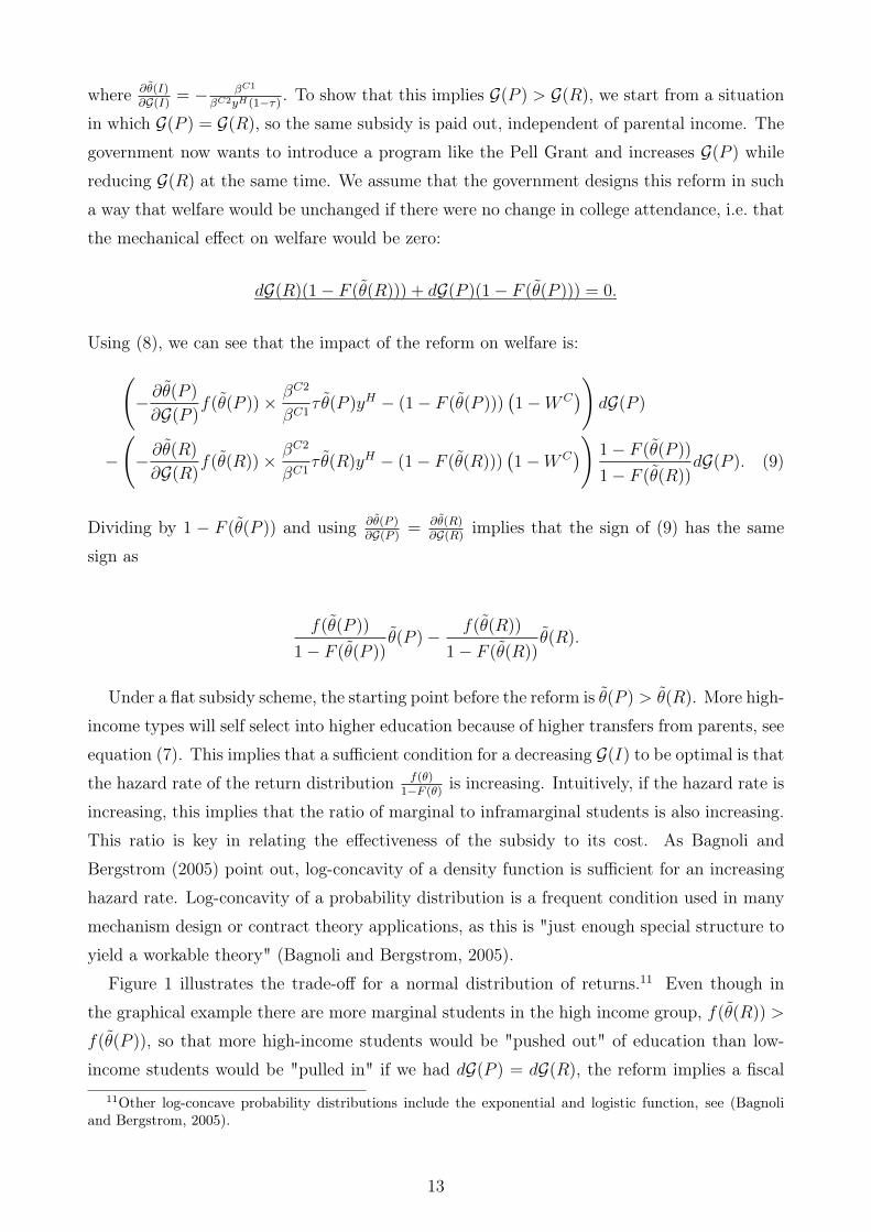
Under a flat subsidy scheme, the starting point before the reform is θ(P ) > θ(R). More high-

income types will self select into higher education because of higher transfers from parents, see

equation (7). This implies that a sufficient condition for a decreasing G(I) to be optimal is that

the hazard rate of the return distribution f(θ)1−F (θ)

is increasing. Intuitively, if the hazard rate is

increasing, this implies that the ratio of marginal to inframarginal students is also increasing.

This ratio is key in relating the effectiveness of the subsidy to its cost. As Bagnoli and

Bergstrom (2005) point out, log-concavity of a density function is sufficient for an increasing

hazard rate. Log-concavity of a probability distribution is a frequent condition used in many

mechanism design or contract theory applications, as this is "just enough special structure to

yield a workable theory" (Bagnoli and Bergstrom, 2005).

Figure 1 illustrates the trade-off for a normal distribution of returns.11 Even though in

the graphical example there are more marginal students in the high income group, f(θ(R)) >

f(θ(P )), so that more high-income students would be "pushed out" of education than low-

income students would be "pulled in" if we had dG(P ) = dG(R), the reform implies a fiscal11Other log-concave probability distributions include the exponential and logistic function, see (Bagnoli

and Bergstrom, 2005).

13

surplus. The reason is that dG(P ) is scaled up by 1−F (θ(P ))

1−F (θ(R))as compared to G(P ). Because

of the increasing hazard ratio assumption the increase in the number of low parental income

students due to the reform is larger than the decrease in the number of high parental income

students.

(R) (P )Returns

f()

PDF: Low-Income

PDF: High-Income

(R) (P )Returns

f()

1

Figure 1: Illustration of progressivity result if parental income and returns are iid.

The model ignores three mechanisms which would lead to a higher progressiveness. First,

borrowing constraints for lower income households naturally would give the government an

incentive to provide liquidity with financial aid. Second, a higher welfare weight placed on

low-income students would give a redistributive gain. Third, suppose there are utility costs of

attending college which differ across income groups. Such utility costs are known as psychic

costs in the empirical literature. If the utility costs is correlated with parental income such

that they are higher for the low-income group, this re-enforces the mechanisms described

above. The reason is that in this model the marginal θ type will be shifted to the left even

further in the high-income distribution, as there is more self-selection of this group.

However, the model also ignores mechanisms that might work against the need-based result.

As Carneiro and Heckman (2003, p.27) write: "Family income and child ability are positively

correlated, so one would expect higher returns to schooling for children of high- income families

for this reason alone." In a famous paper, Altonji and Dunn (1996) find higher returns to

schooling for children with more-educated parents than for children with less-educated parents.

Whereas the simple model provides an interesting and intuitive benchmark, a richer empir-

ical model is needed to answer the question for the question of how need-based financial aid

policies should be. In the next section we set up such a model and quantify it for the U.S.

14

4 Estimation and Calibration of Full Model

Although plausible, the theoretical result that progressive subsides are efficient relies on func-

tional form assumptions. For this reason, and to obtain quantitative insights, we now move

to our empirical model. We first explain how we concretely specify the model in Section 4.1.

In Section 4.2 we explain how we quantify the model using micro data and information on

current policies. In Section 4.3 we show in detail that the quantitative model performs very

well in replicating patterns in the data and quasi-experimental evidence on returns to college

and the elasticity of college education with respect to financial aid.

4.1 Empirical Model Specification

We now specify the concrete set-up for the empirical model. Concerning the underlying het-

erogeneity, in addition to parental income the main variables of interest are ability θ and

psychic costs κ. Importantly, we allow for any correlation structure between parental income,

ability, and the psychic costs of attending college. We will use other information like parental

education, race, and location to improve the fit of the model – the details are found below in

the estimation description. We assume that ability directly influences the wage distribution,

i.e. we specify the wage distributions as GC(w|θ) and GH(w|θ). We assume these functions

to be independent of parental income because we did not find a strong significant effect of

parental income.

Psychic costs an be interpreted as a one-dimensional aggregate that captures factors that

influence the decision to go to college beyond the budget constraint. Taking into account the

psychic costs of education has been shown to be very important because monetary returns can

only account for a small part of the observed college attendance patterns (Cunha et al., 2005;

Heckman et al., 2006; Johnson, 2013). This is also true in our model as unreported estimation

results show: not allowing for psychic costs that vary with ability and parental characteristics

would imply that we cannot match well the cross-sectional college graduation patterns. As is

standard in the literature, they enter the model additively.

Given these assumptions, the value functions in case of college attendance is

V C(I, θ;G(·), T (·)) = maxcCj ,c

Wjw,y

Ww

βC1UC(cCj ) + βC2

∫Ω

UW(cWjw, y

Ww ;w

)dGC(w|θ) (10)

subject to

∀ w : cWjw = yWjw − T (yWw )− (1 + r)L

cCj = trC(I) + G(.)− C + L,

15

L ≤ L,

where j is a realization of the triple (I, θ). Psychic costs (which can also take negative values,

i.e. be psychic benefits) κ are just subtracted from the value function. For the flow utility

function, we assume (for both high-school and college graduates)

(C − ( yw)

1+ε

1+ε

)1−γ

1− γ.

which implies that labor income y only depends on w. So we make the standard assumption

that preferences over consumption and work are homogenous. Consumption in college differs

because of heterogeneity in parental transfers, financial aid receipt, and borrowing. We assume

that agents are borrowing constrained and can only borrow up to L but show that our policy

implications are not altered if agents can freely borrow. For high-school graduates, we have:

V H(I, θ;T (.)) = maxcHw ,y

Hw

βH∫

Ω

UH(cHw , y

Hw ;w

)dGH(w|θ) (11)

subject to

∀ w : cHw = yHw − T (yHw ) + trH(I).

An individuals of type (θ, I, κ) goes to college if V C(I, θ;G(·), T (·))−κ ≥ V H(I, θ;T (.)). This

implies that we can capture the college margin w.r.t. policies by a simple threshold function

κ(θ, I) = V C(I, θ;G(·), T (·))− V H(I, θ;T (.)).

An important simplifying assumption that we make is to abstract from the direct modeling

of labor supply behavior over the life-cycle because we are mostly interested in getting the

net-present value of the fiscal externalities over the life-cycle right. This is achieved by using

annuity values of the average discounted sums of income, as we describe below. Such simpli-

fications are also commonly made in other calculations, calculating the lifetime present value

effects of policies on earnings in the literature, for example in Chetty et al. (2014) and Kline

and Walters (2016).

4.2 Data & Procedure

To bring our model to the data, we make use of the National Longitudinal Survey of the Youth

97 (henceforth NLSY97). A big advantage of this data set is that it contains information

on parental income and the Armed Forced Qualification Test Score (AFQT-score) for most

individuals. The latter is a cognitive ability score for high-school students that is conducted

by the US army. The test score is a good signal of ability. Cunha et al. (2011), e.g., show that

it is the most precise signal of innate ability among comparable scores in other data sets.

16

Table 1: Parameters and Targets

Object Description Procedure/Target

F (I) Marginal distribution of parental income Directly taken from NSLY97(θ, I) Joint and conditional distribution of innate abilities Directly taken from NSLY97GH(w|θ) Conditional Wage Distribution High-school Estimated from regressionsGC(w|θ) Conditional Wage Distribution College Estimated from regressionstrH(I) Conditional Transfer Distribution High-school Estimated from regressionstrC(I) Conditional Transfer Distribution College Estimated from regressionsK(θ, I, κ) Joint distributions with psychic costs Maximum Likelihood

Utility Function:(C− l1+ε

1+ε

)1−γ

1−γ

ε=0.5 Labor Supply Elasticity Chetty et al. (2011)γ=1.85 Curvature of Utility Enrollment Elasticities

Current Policies

L Stafford Loan Maximum Value in year 2000T (y) Current Tax Function Gouveia-Strauss (Guner et al., 2014)G(θ, I) Need- and Merit-Based Grants Estimated from regressions

Since individuals in the NLSY97 are born between 1980 and 1984, not enough information

about their earnings is available. We therefore also use the NLSY79 as this data set contains

more information about labor market outcomes – individuals are born between 1957 and 1964.

Combining both data sets in such a way has proven to be a fruitful way in the literature to

overcome the limitations of each individual data set, see Johnson (2013) and Abbott et al.

(2016). The underlying assumption is that the relation between AFQT and wages has not

changed over that time period. We use the method of Altonji et al. (2012) to make the

AFQT-scores comparable between the two samples and different age groups.

Finally, we define an individual as a college graduate if she has completed at least a bache-

lor’s degree. Otherwise she counts as a high school graduate. Since individuals in the NLSY97

turn 18 years old between 1998 and 2002, we express all US-dollar amounts in year 2000 dollars.

An overview of our calibration and estimation procedure is given in Table 1. First of all,

to quantify the joint distribution of parental income and ability, we take the cross-sectional

joint distribution in the NLSY97. We then proceed in 4 steps:

1. We calibrate and preset a few parameters in Section 4.2.1.

2. We calibrate current U.S. tax and college policies in Section 4.2.2.

3. We estimate trC(I), trH(I), GC(w|θ) and GH(w|θ) with simple regressions in Sec-

tion 4.2.3.

17

4. Based on that, we calculate V C(I, θ;G(.), T (.)) and V H(I, θ;T (.)) for each individual

and estimate the distribution of psychic costs with maximum likelihood in Section 4.2.4.

4.2.1 Calibrated Parameters

We assume that college takes 4.5 years (i.e. Te = 4.5) and assume that individuals spend 43.5

or 48 years on the labor market depending on whether they went to college. The choice of

4.5 years for degree completion corresponds to the average years to graduation we observe in

the NLSY97, which is 4.57 years. This lines up well with numbers from other sources, for

example, from the National Center for Education Statistics (NCES).12 We set the risk-free

interest rate to 3%, i.e. R = 1.03 and assume that individuals’ discount factor is β = 1R.

For the labor supply elasticity, we choose ε = 2, which implies a compensated labor supply

elasticity of .513 Note that the value of the labor supply elasticity does not influence our results

for given taxes because we calibrate wages from elasticities and income as in Saez (2001). We

are more explicit about that in Section 4.2.3. The value of the curvature parameter γ matters

for the elasticity of the college education decision. We set γ = 1.85 as this implies an elasticity

in the mid range of estimates from the empirical literature. We comment on that more in

Section 4.3.

4.2.2 Calibration of Current Policies

To capture current tax policies, we use the approximation of Guner et al. (2014), which

has been shown to work well in replicating the US tax code. More details are contained in

Appendix A.2.1.

For tuition costs, we take average values for the year 2000 from Snyder and Hoffman

(2001) for the regions North East, North Central, South and West, as they are defined in the

NLSY. We also take into account the amount of money that is spent per student by public

appropriations, which has to be taken into account for the fiscal externality. Both procedures

are described in detail in Appendix A.2.2. The average values are $7,434 for annual tuition

and $4,157 for the annual public appropriations per student.

Besides these implicit subsidies, students receive explicit subsidies in the form of grants and

tuition waivers. We estimate how this grant receipt varies with parental income and ability in

Appendix A.2.5 using information provided in the NLSY97. We find a strong negative effect of

parental transfers on financial aid receipt at the extensive and intensive margin. Additionally,

we can capture merit-based grants by the conditional correlation of AFQT scores with grant

receipt.12See http://nces.ed.gov/fastfacts/display.asp?id=569.13Micro-evidence suggests that the compensated elasticity is probably lower, around .33 (Chetty et al.,

2011), Given that our elasticity reflects the labor supply responsiveness over the life cycle, we take a largervalue of .5.

18

Finally, we make the assumption that individuals can only borrow through the public

loan system. In the year 2000, the maximum amount for Stafford Loans per student was

$23,000. The latter assumption does not seem innocuous. For our results about the desirability

of increasing college subsidies, it is rather harmless because we show how our results can

be understood in terms of sufficient statistics and our quantified model is targeted to the

respective quasi-experimental evidence (by choosing the parameter γ). Further, we show that

our main result about the progressivity of optimal financial aid prevails if we allow for free

borrowing in Section 5.3.

4.2.3 Reduced Form Regressions

Wage Distributions. In our model, y refers to an average income over the lifetime as

we only have one labor market period. Therefore, we take annuitized income as the data

counterpart. Our approach to estimate the relationship between innate ability, education and

labor market outcomes relates to Abbott et al. (2016) and Johnson (2013). We run regressions

of log annuitized income on AFQT for both education levels. This gives us conditional log-

normal distributions of labor income (see Appendix A.2.3 for details).

Top incomes are underrepresented in the NLSY as in most survey data sets. Following

common practice in the optimal tax literature (Piketty and Saez, 2013), we therefore append

Pareto tails to each income distribution, starting at incomes of $350,000. We set the shape

parameter a of the Pareto distribution to 2 for all income distributions.14 Figure 12(a) in

Appendix A.1 shows the expected annual before tax income as a function of the AFQT (in

percentiles) for both education levels and clearly demonstrates the complementarity between

innate ability and education, which has also been highlighted in previous papers (Carneiro and

Heckman, 2003). The red bold line in Figure 12(b) in Appendix A.1 shows how this translates

into an expected NPV difference in lifetime earnings. As was argued in the theoretical section,

the returns to education play an important role for the fiscal effects of an increase in college

enrollment. The additional tax payment (again in NPV) is clearly increasing in AFQT (black

dotted line). To get the overall impact on the government budget, subsidies have to be

subtracted, which are given by the black dashed-line. Subsidies are increasing in ability which

reflects the fact that individuals with higher ability currently obtain higher scholarships (merit-

based financial aid), which we elaborate in Section A.2.5. The net impact on public funds is

given by the blue dashed-dotted line.14Diamond and Saez (2011) find that starting from ≈ $350, 000 the Pareto parameter is constant and

1.5. Since their data are for 2005 and our data are also for earlier periods, we choose a Pareto parameterof 2 because top incomes were less concentrated earlier. The rationale for having the Pareto parameterindependent of education and innate ability is that we did not find any systematic relationship between thePareto parameter and either θ or education in the NLSY.

19

The last step consists of calibrating the respective skill/wage distribution from the income

distributions by exploiting the first-order condition of individuals as pioneered by Saez (2001).

This highlights that our results for an exogenous tax function are independent of the labor

supply elasticity. The wages are always calibrated such that they produce the income distribu-

tion that we estimated. If we change the value of the elasticity, the wages adjust accordingly.

For our results on optimal taxes that we study in Section 6, the labor supply elasticity matters

of course – the higher it is the lower are optimal taxes. However, it does not have significant

consequences for the optimal progressivity of financial aid as we find in unreported simulation

exercises.

Parental Transfers. For brevity, details of the estimation are relegated to Appendix A.2.4.

Economically, the most important results for parental transfers is the strong dependence on

education choice by the child. This contingency of parental transfers acts as a price subsidy

for college. On top, we recover the well-known positive correlation between parental income

and transfers.

4.2.4 Structural Estimation of Psychic Costs

Based on the estimated reduced form relationships, we can calculate the two value functions

(10) and (11) for each individual in the NLSY97 – after dropping individuals for whom the

relevant information is not known, we are left with 3,897 individuals. In line with the empirical

literature, we assume that the decision to go to college is also influenced by heterogeneity in

preferences for college. We assume that these psychic costs are determined by parental educa-

tion and by innate ability – see Cunha et al. (2005), among others.15 To achieve identification,

we impose a normality assumption on the distribution of preferences. The model is estimated

as a standard discrete choice model with maximum-likelihood and details of the procedure

are found in Appendix A.2.6. As expected, higher ability and parental education increase

the non-pecuniary benefits from college (i.e. lower the psychic costs). As shown in the fol-

lowing Section 4.3, the estimated model performs very well in replicating quasi-experimental

evidence.

4.3 Model Performance and Relation to Empirical Evidence

In order to assess the suitability of the model for policy analysis, we look at how well it

replicates well-known findings from the empirical literature and especially quasi-experimental

studies.15The literature also suggests that individuals that grew up in urban areas are more likely to go to college.

The coefficient did not turn out as significant in our estimation and we therefore do not include it in ouranalysis. The inclusion of the variable does not affect any of our results.

20

Graduation Shares. Figure 2 illustrates graduation rates as a function of parental income

and AFQT in percentiles respectively. The bold lines indicate results from the model and the

dashed lines are from the data. We slightly underestimate the parental income gradient. The

correlation between AFQT and college graduation, however, is well-fitted. The overall number

of individuals with a bachelor degree is 30.56% in our sample and 30.85% in our model. Data

from the United States Census Bureau are very similar: the share of individuals aged 25-29

in the year 2009 holding a bachelor degree is 30.6% – this comes very close to our data, where

we look at cohorts born between 1980 and 1984.

0 0.2 0.4 0.6 0.8 1Parental Income Percentile

0

0.1

0.2

0.3

0.4

0.5

0.6

0.7

Sh

are

of

Co

lleg

e G

rad

ua

tes

ModelData

(a) Graduation Rates and Parental Income

0 20 40 60 80 100AFQT-Percentile

0

0.1

0.2

0.3

0.4

0.5

0.6

0.7

0.8

Sh

are

of

Co

lleg

e G

rad

ua

tes

ModelData

(b) Graduation Rates and AFQT

Figure 2: Graduation Rates

Responsiveness of Graduation to Grant Increases. Many papers have analyzed the

impact of increases in grants or decreases in tuition on college enrollment. Kane (2006)

and Deming and Dynarski (2009) survey the literature. The estimated impacts of a $1,000

increase in yearly grants (or a respective reduction in tuition) on enrollment ranges from 1-6

percentage points, depending on the policy reform and research design. Numbers differ since

some of the evaluated programs were targeted towards low-income groups and others were

not, and sometimes the higher amount of grants was associated with a lot of paperwork,

which might create selection. The majority of studies arrive at numbers between 3 and 5

percentage points, however. As our model is a model of college graduation instead of college

enrollment, the numbers are not directly comparable for two reasons: (i) not all of the newly

enrolled students will indeed graduate with a bachelor’s degree, (ii) some of the newly enrolled

students enroll in community colleges and (iii) students that have enrolled also for lower grants

are less likely to drop out of college. Relatively little is known about (iii). Concerning (i), we

know that in the year 2000 roughly 66% of newly enrolled students enroll in 4-year institutions

(Table 234 of Snyder and Dillow (2013)). Of those 66%, only slightly more than half should

be expected to graduate with a bachelor’s degree. We estimate that the dropout probability

21

of the marginal students in our model is 45%. However, of those initially enrolled at two-year

colleges, also 10% graduate with a bachelor’s degree (Shapiro et al. 2012, Figure 6). Thus,

translating the 3-5 percentage points increase in enrollment into numbers for graduation rates,

we get 1.2-2 percentage points when taking into account (i) and (ii). Taking into account

(iii) would yield slightly higher numbers. However, there is no strong empirical evidence on

this effect that would guide us about the quantitative importance. We chose the parameter

γ = 1.85 of the utility function such that we are exactly in the middle of this range at 1.6.

A more recent study by Castleman and Long (2016) looks at the impact of grants targeted

to low-income children. Applying a regression-discontinuity design for need-based financial

aid in Florida (Florida Student Access Grant), they find that a $1,000 increase in yearly

grants for children with parental income around $30,000 increases enrollment by 2.5 percentage

points. Interestingly, they find an even larger increase in the share of individuals that obtain a

bachelor’s degree after 6 years by 3.5 percentage points. After 5 years the number is also quite

high at 2.5 percentage points. These results show that grants can have substantial effects on

student achievement after enrollment.

Importance of Parental Income. It is a well-known empirical fact that individuals with

higher parental income are more likely to receive a college degree, see also Figure 2(a). How-

ever, it is not obvious whether this is primarily driven by parental income itself or variables

correlated with parental income and college graduation. Using income tax data and a research

design exploiting parental layoffs, Hilger (2016) finds that a $1,000 increase in parental income

leads to an increase in college enrollment of .43 percentage points. Using a similar back of the

envelope calculation as in the previous paragraph – i.e. that a 1 percentage point enrollment

increase leads to a .40 percentage points increase in graduation rates – this implies an increase

in graduation rates of .17 percentage points. To test our model, we increased parental income

for each individual by $1,000 and obtained increases in bachelor’s completion by 0.08 percent-

age points. In line with Hilger (2016), our model predicts a very moderate effect of parental

income, smaller but in line with Hilger (2016).

The College Wage Premium and Marginal Returns. The college-earnings premium

in our model is 99%, i.e. the average income of a college graduate is twice as high as the

average income of a high-school graduate. As our earnings data are for the 1990s and the

2000s, this is well in line with empirical evidence in Oreopoulos and Petronijevic (2013); see

also Lee et al. (2014). Doing the counterfactual experiment and asking how much the college

graduates would earn if they had not gone to college, we find that the returns to college are

62.9%. This implies a return of 12.43% for one year of schooling, which is in the upper half

22

of the range of values found in Mincer equations (Card, 1999; Oreopoulos and Petronijevic,

2013).16

The more important number for our analysis is the return to college for marginal students.

We find it to be slightly lower at 58.62%, which implies a return to one year of schooling of

11.53%. This reflects that marginal students are of lower ability on average than inframarginal

students and is also in line with Oreopoulos and Petronijevic (2013). A clean way to infer

returns for marginal students is found in Zimmerman (2014). In his study, students are

marginal w.r.t. academic ability, measured by a GPA admission cutoff. He finds returns of

about 9.9% per year.17 However, since his number refer to the academically marginal students

with GPA’s around 3, whereas in our thought experiment we refer to those students who are

marginal w.r.t. a small change in financial aid, these students are likely to be of higher ability

than the academically marginal students. We explore this issue and make use of the fact that

the NLSY also provides GPA data. In fact, our model gives a return to college of 51.73% for

students with a GPA in the neighborhood of 3, which implies a Mincer return of 10.42% for

one year of schooling – which comes very close to the 9.9% from Zimmerman (2014).

Finally, we do not account for differing rates of unemployment and disability insurance

rates. Both numbers are typically found to be only half as large for college graduates (see

Oreopoulos and Petronijevic (2013) for unemployment and Laun and Wallenius (2016) for

disability insurance). Further, the fiscal costs of Medicare are likely to be much lower for

individuals with college degree. Lastly, we assume that all individuals work until 65 not taking

into account that college graduates on average work longer (Laun and Wallenius, 2016). These

facts would generally strengthen the case for an increase in college subsidies.

The Role of Borrowing Constraints. To assess the importance of borrowing constraints,

we completely remove them and ask by how much graduation increases. In this experiment,

enrollment increases by 3.94 percentage points from 30.85% to 34.79%. This value is in the

realm of values the literature has found, see, e.g., Johnson (2013) and Navarro (2011). This

significant enrollment increase due to the removal of borrowing constraints is also in line

with Belley and Lochner (2007) who find, based on NLSY data, that borrowing constraints

are likely to have become more stringent. As Figure 13(a) in Appendix A.1 reveals, the

removal of borrowing constraints has larger effects for low-income children. Figure 13(b) in

Appendix A.1 illustrates the importance of borrowing constraints for individuals with different16The calculation is as follows. In a Mincer regression, the log of earnings is regressed on years of schooling.

The difference in log(1.64y) and log(y) is equal to log(1.64). Dividing by four years of schooling (for a bachelor’sdegree) yields 12.20% per year of schooling.

17He finds gains of 22% to obtain four-year college admission, which should be compared to the returnof community colleges, which are the most frequent outside options for those students and take on averageabout 2 year less to complete. In addition, his findings are for earnings around 8 and 14 years after highschool completion. Given that college students have a steeper earnings profile (see, e.g., Lee et al. 2014), thesenumbers are likely to underestimate the return to lifetime earnings.

23

innate abilities. Naturally, individuals with high ability have the strongest need for more

borrowing because of high expected future earnings.

5 Results: Optimal Financial Aid

We now present our main quantitative results. After the benchmark in Section 5.1, we show

that results are robust to the welfare function and also hold if the government only wants to

maximize tax revenue in Section 5.2. One might think that results are driven by borrowing

constraints. As we show in Section 5.3, even if a perfect credit market could be provided,

the optimal financial aid schedule is strongly progressive. In Section 5.4, we also chose the

need-based element optimal and find that this does not alter our result at all. We show that

a larger degree of progressivity can be implemented in a Pareto improving way in Section 5.5.

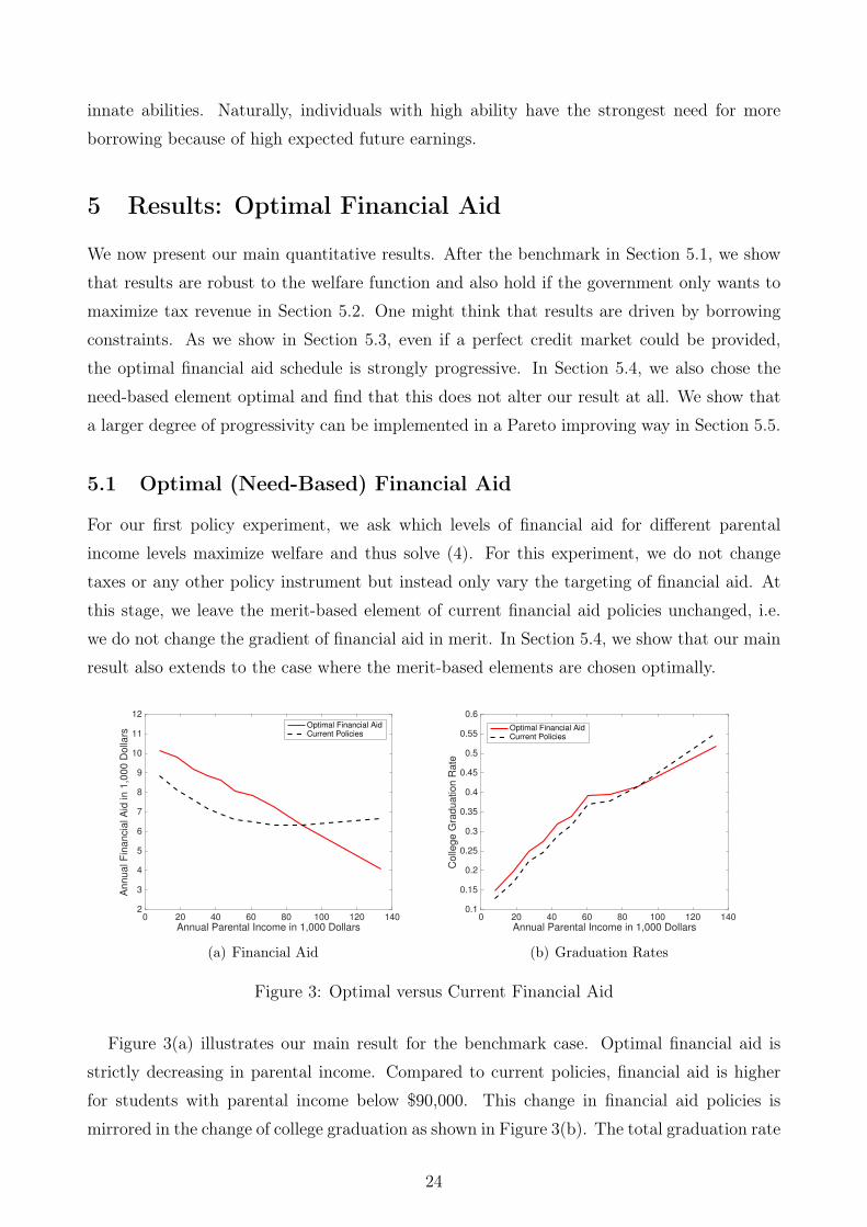
5.1 Optimal (Need-Based) Financial Aid

For our first policy experiment, we ask which levels of financial aid for different parental

income levels maximize welfare and thus solve (4). For this experiment, we do not change

taxes or any other policy instrument but instead only vary the targeting of financial aid. At

this stage, we leave the merit-based element of current financial aid policies unchanged, i.e.

we do not change the gradient of financial aid in merit. In Section 5.4, we show that our main

result also extends to the case where the merit-based elements are chosen optimally.

0 20 40 60 80 100 120 140Annual Parental Income in 1,000 Dollars

2

3

4

5

6

7

8

9

10

11

12

An

nu

al F

ina

ncia

l A

id in

1,0

00

Do

llars

Optimal Financial AidCurrent Policies

(a) Financial Aid

0 20 40 60 80 100 120 140Annual Parental Income in 1,000 Dollars

0.1

0.15

0.2

0.25

0.3

0.35

0.4

0.45

0.5

0.55

0.6

Co

lleg

e G

rad

ua

tio

n R

ate

Optimal Financial AidCurrent Policies

(b) Graduation Rates

Figure 3: Optimal versus Current Financial Aid

Figure 3(a) illustrates our main result for the benchmark case. Optimal financial aid is

strictly decreasing in parental income. Compared to current policies, financial aid is higher

for students with parental income below $90,000. This change in financial aid policies is

mirrored in the change of college graduation as shown in Figure 3(b). The total graduation rate

24

increases by 1.6 percentage points to 32.44%. This number highlights the efficient character

of this reform.

Why Are Optimal Policies So Progressive? A Decomposition. We now illustrate

what drives the progressivity result. From the optimality condition

∂FC(I)

∂G(I)×∆T (I)− FC(I)× (1−WC(I)) = 0

we plot each of the components evaluated at the optimal system. Figure 4(a) plots the share

of marginal students ∂FC(I)∂G(I)

against parental income in the optimal system. It actually shows

0 20 40 60 80 100 120 140Annual Parental Income in 1,000 Dollars

0.0115

0.012

0.0125

0.013

0.0135

0.014

0.0145

0.015

0.0155

0.016

0.0165

Sh

are

Share of Marginal Students for $1,000 Increase

(a) Marginal Students

0 20 40 60 80 100 120 140Annual Parental Income in 1,000 Dollars

20

30

40

50

60

70

80

90

100

Do

llar

in 1

,00

0

Average Expected Fiscal Externality

(b) Fiscal Externality

Figure 4: Marginal Students and Fiscal Externality in Optimal System

an increasing share of marginal students but the relative differences are small as the share

increases from 1.2% to around 1.6%. This works against our progressivity result. Figure 4(b)

shows the implied average fiscal externality at the optimal system. It increases by a factor

around 3 from $30,000 to $100,000. This implies that also the shape of ∆T (I) works against

the progressivity result because marginal students from higher income households have higher

returns. Figure 5(a) plots the share of inframarginal students, showing that even in the optimal

system there is a strong parental income gradient, as the share increases from around 12% to

around 55% implying a factor of around 4.5. Finally, Figure 5(b) shows the implied marginal

welfare weights at the optimum. They imply that 1−WC(I), which is the relevant term for

the formula, increases from around 0.5 to around 0.7 at the top, so by a factor of around

1.4. Taken together, the decomposition yields that the share of inframarginal students is key

in explaining the progressivity result. Although marginal students from higher incomes have

higher returns to college, working against progressive aid policies, this is overturned by the fact

that college attendance is still highly correlated with parental resources. Put differently, even

25

0 20 40 60 80 100 120 140Annual Parental Income in 1,000 Dollars

0.1

0.15

0.2

0.25

0.3

0.35

0.4

0.45

0.5

0.55

0.6

Sh

are

Share of Infra-Marginal Students

(a) Inframarginal Students

0 20 40 60 80 100 120 140Annual Parental Income in 1,000 Dollars

0.32

0.34

0.36

0.38

0.4

0.42

0.44

0.46

0.48

0.5

In t

erm

s o

f p

ub

lic f

un

ds

Marginal Social Welfare Weight

(b) Marginal Welfare Weights

Figure 5: Inframarginal Students and Welfare Weights in Optimal System

though a progressive system subsidizes low-income children much more, high-income children

are still more likely to attend college.

5.2 Tax-Revenue Maximizing Financial Aid

One might be suspicious of whether the progressivity is driven by a desire for redistribution

from rich to poor students. If this were the case, the question would naturally arise whether the

financial aid system is the best means of doing so. However, we now show that the result even

holds in the absence of redistributive purposes. We ask the following question: how should a

government that is only interested in maximizing tax revenue (net of expenditures for financial

aid) set financial aid policies? Figure 6(a) provides the answer: revenue maximizing financial

aid in this case is very progressive as well. Whereas the overall level is naturally lower if the

consumption utility of students is not valued, the declining pattern is basically unaffected.

For lower parental income levels, revenue maximizing aid is even above the current one which

implies that an increase must be more than self-financing. We study this in more detail in

Section 5.5. The implied graduation patterns are illustrated in Figure 6(b).

5.3 The Role of Borrowing Constraints

We have shown that the optimal progressivity is not primarily driven by redistributive tastes

but rather by efficiency considerations. Given that our analysis assumes that students cannot

borrow more than the Stafford Loan limit, the question arises whether these efficiency consid-

erations are driven by borrowing limits that should be particularly binding for low parental

income children.

To elaborate upon this question, we ask how normative prescriptions for financial aid

policies change if students can suddenly borrow as much as they want. As illustrated in

26

0 20 40 60 80 100 120 140Annual Parental Income in 1,000 Dollars

2

3

4

5

6

7

8

9

10

11

12

An

nu

al F

ina

ncia

l A

id in

1,0

00

Do

llars

Revenue Maximizing AidOptimal Financial AidCurrent Policies

(a) Financial Aid

0 20 40 60 80 100 120 140Annual Parental Income in 1,000 Dollars

0.1

0.15

0.2

0.25

0.3

0.35

0.4

0.45

0.5

0.55

0.6

Co

lleg

e G

rad

ua

tio

n R

ate

Revenue Maximizing AidOptimal Financial AidCurrent Policies

(b) Graduation Rates

Figure 6: Tax Revenue Maximizing Financial Aid Policies

Figure 7(a), optimal financial aid policies become even more progressive in this case. The

abolishment of borrowing constraints implies a boost in college education which implies a

large increase in tax revenue that can now be used to increase financial aid. The increase is

mainly targeted at low parental income children. First, because of their higher welfare weight.

Second, because also in the absence of borrowing constraint, the general force that subsidizing

low parental income children is relatively cost-effective survives because of the much lower

share of inframarginal students as can be seen in Figure 7(b).

0 20 40 60 80 100 120 140Annual Parental Income in 1,000 Dollars

2

4

6

8

10

12

14

16

An

nu

al F

ina

ncia

l A

id in

1,0

00

Do

llars

Optimal Financial Aid + Free BorrowingOptimal Financial AidCurrent Policies

(a) Financial Aid

0 20 40 60 80 100 120 140Annual Parental Income in 1,000 Dollars

0.1

0.15

0.2

0.25

0.3

0.35

0.4

0.45

0.5

0.55

0.6

Co

lleg

e G

rad

ua

tio

n R

ate

Optimal Financial Aid + Free BorrowingOptimal Financial AidCurrent Policies

(b) Graduation Rates

Figure 7: Financial Aid and Graduation with Free Borrowing

5.4 Merit-Based Financial Aid

Up to now, we have assumed that the merit-based element of financial aid policies stays

unaffected. We now allow the government to optimally choose the gradient in merit and

parental income. Figure 8(a) shows that – if optimally targeted also in terms of merit –

27

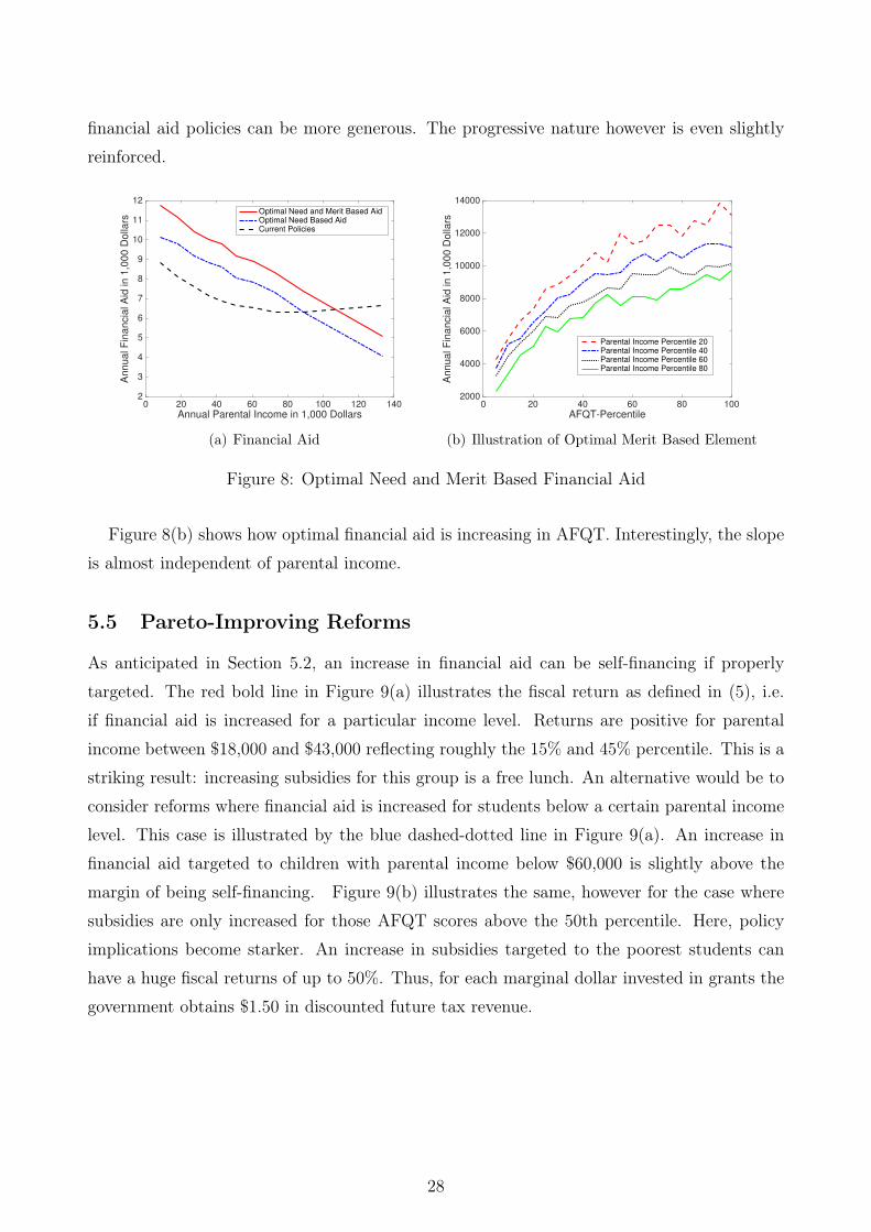
financial aid policies can be more generous. The progressive nature however is even slightly

reinforced.

0 20 40 60 80 100 120 140Annual Parental Income in 1,000 Dollars

2

3

4

5

6

7

8

9

10

11

12

An

nu

al F

ina

ncia

l A

id in

1,0

00

Do

llars

Optimal Need and Merit Based AidOptimal Need Based AidCurrent Policies

(a) Financial Aid

0 20 40 60 80 100

AFQT-Percentile

2000

4000

6000

8000

10000

12000

14000

An

nu

al F

ina

ncia

l A

id in

1,0

00

Do

llars

Parental Income Percentile 20Parental Income Percentile 40Parental Income Percentile 60Parental Income Percentile 80

(b) Illustration of Optimal Merit Based Element

Figure 8: Optimal Need and Merit Based Financial Aid

Figure 8(b) shows how optimal financial aid is increasing in AFQT. Interestingly, the slope

is almost independent of parental income.

5.5 Pareto-Improving Reforms

As anticipated in Section 5.2, an increase in financial aid can be self-financing if properly

targeted. The red bold line in Figure 9(a) illustrates the fiscal return as defined in (5), i.e.

if financial aid is increased for a particular income level. Returns are positive for parental

income between $18,000 and $43,000 reflecting roughly the 15% and 45% percentile. This is a

striking result: increasing subsidies for this group is a free lunch. An alternative would be to

consider reforms where financial aid is increased for students below a certain parental income

level. This case is illustrated by the blue dashed-dotted line in Figure 9(a). An increase in

financial aid targeted to children with parental income below $60,000 is slightly above the

margin of being self-financing. Figure 9(b) illustrates the same, however for the case where

subsidies are only increased for those AFQT scores above the 50th percentile. Here, policy

implications become starker. An increase in subsidies targeted to the poorest students can

have a huge fiscal returns of up to 50%. Thus, for each marginal dollar invested in grants the

government obtains $1.50 in discounted future tax revenue.

28

0 20 40 60 80 100 120 140Parental Income in 1,000

-50

-40

-30

-20

-10

0

10

20

30

40

50

Re

turn

in

%Targeted to Parental Income XProfitability ThresholdTargeted to Parental Incomes Lower or Equal X

(a) All Ability Levels

0 20 40 60 80 100 120 140Parental Income in 1,000

-50

-40

-30

-20

-10

0

10

20

30

40

50

Re

turn

in

%

Targeted to Parental Income XProfitability ThresholdTargeted to Parental Incomes Lower or Equal X

(b) Targeted to Above Median Ability

Figure 9: Fiscal Returns on Increase in Financial Aid

6 Results: Jointly Optimal Financial Aid and

Income Taxation

The size of the fiscal externality of college education depends on the tax and transfer system

in place. Our stuctural estimates took the current US tax system as given. An interesting

question to ask is how optimal subsidies change when the tax schedule is chosen optimally.

To address this, we enrich the optimal policy space such that the planner can also pick a

nonlinear tax function T (y) as is standard in the public finance literature (Piketty and Saez,

2013).18

First, the optimal formulas for the subsidy schedule are unchanged and still given by the

formulas in Section 2. In Appendix B, we show what the endogenous extensive education

margin implies for optimal marginal tax rates.19 For the sake of brevity, we discuss the

theory only in the Appendix and now move on to the quantitative implications of optimal

taxes. We assume that agents are borrowing constrained and the government only (besides

the tax schedule) maximizes the need-based element of the financial aid schedule. Results are

barely changed if borrowing constraints are relaxed and/or the merit-based element is chosen

optimally as well.

Figure 10(a) displays optimal average tax rates in the optimal as well as in the current US

system. Average tax rates are higher for most part of the income distribution. As Figure 10(b)

shows, this is driven by higher marginal tax rates throughout but especially at the bottom of

the distribution, a familiar result from the literature (Diamond and Saez, 2011). In unreported

results, we find that the direct effect of taxes on enrollment decisions, which we discussed in18We abstract from education dependent taxation; for such cases please see Findeisen and Sachs (2016) and

Stantcheva (2016).19The formula is therefore related to the formulas of Saez (2002) and Jacquet et al. (2013), where the

extensive margin is due to labor market participation, or Lehmann et al. (2014) where the extensive margincaptures migration.

29

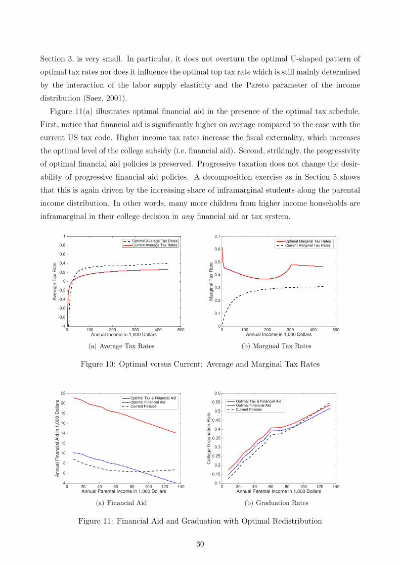
Section 3, is very small. In particular, it does not overturn the optimal U-shaped pattern of

optimal tax rates nor does it influence the optimal top tax rate which is still mainly determined

by the interaction of the labor supply elasticity and the Pareto parameter of the income

distribution (Saez, 2001).

Figure 11(a) illustrates optimal financial aid in the presence of the optimal tax schedule.

First, notice that financial aid is significantly higher on average compared to the case with the

current US tax code. Higher income tax rates increase the fiscal externality, which increases

the optimal level of the college subsidy (i.e. financial aid). Second, strikingly, the progressivity

of optimal financial aid policies is preserved. Progressive taxation does not change the desir-

ability of progressive financial aid policies. A decomposition exercise as in Section 5 shows

that this is again driven by the increasing share of inframarginal students along the parental

income distribution. In other words, many more children from higher income households are

inframarginal in their college decision in any financial aid or tax system.

Annual Income in 1,000 Dollars0 100 200 300 400 500

Ave

rag

e T

ax R

ate

-1

-0.8

-0.6

-0.4

-0.2

0

0.2

0.4

0.6

0.8

1Optimal Average Tax RatesCurrent Average Tax Rates

(a) Average Tax Rates

0 100 200 300 400 500Annual Income in 1,000 Dollars

0

0.1

0.2

0.3

0.4

0.5

0.6

0.7

Ma

rgin

al T

ax R

ate

Optimal Marginal Tax RatesCurrent Marginal Tax Rates

(b) Marginal Tax Rates

Figure 10: Optimal versus Current: Average and Marginal Tax Rates

0 20 40 60 80 100 120 140Annual Parental Income in 1,000 Dollars

4

6

8

10

12

14

16

18

20

22

An

nu

al F

ina

ncia

l A

id in

1,0

00

Do

llars

Optimal Tax & Financial AidOptimal Financial AidCurrent Policies

(a) Financial Aid

0 20 40 60 80 100 120 140Annual Parental Income in 1,000 Dollars

0.1

0.15

0.2

0.25

0.3

0.35

0.4

0.45

0.5

0.55

0.6

Co

lleg

e G

rad

ua

tio

n R

ate

Optimal Tax & Financial AidOptimal Financial AidCurrent Policies

(b) Graduation Rates

Figure 11: Financial Aid and Graduation with Optimal Redistribution

30

7 Further Aspects

In this section we argue that the result about the progressive nature of optimal student

financial aid is unlikely to change if college dropout, general equilibrium effects on wages,

income effects and parental incentives are taken into account.

Dropout In our analysis we assumed that anybody who goes to college indeed graduates.

Shapiro et al. (2012, Table 6) document that for the cohort which was first enrolled in a

four-year college in the fall of 2006, 62% graduated 6 years later. Thus, at most 38% never

received a bachelor’s degree. So one might wonder to what extent our results are robust to the

incorporation of dropout. If one thinks about the optimality condition (4), what is changed?

(i) The marginal costs of the reform are increased because the increase in subsidies now must

also be paid for students that are inframarginal but do not graduate. If, for example, 38%

are dropouts and they stay in college for two years on average, the marginal cost term –

abstracting from discounting – is increased by 50% (obtained from 0.380.62

24.5

). (ii) An increase

in college subsidies does not only imply marginal students that graduate but also marginal

students that dropout. Note that for our quantitative part we did not make the mistake of

assuming that every additionally enrolled student graduates. Instead, we were only taking into

account the share of those that actually graduate, see also our discussion in Section 4.3. Taking

into account that higher subsidies in addition induce marginal students that dropout might

make an increase of grants more or less desirable depending on whether the college dropouts

contribute more to public funds over their lifecycle than they would have in the absence of any

college education. According to Lee et al. (2014), the earnings premium for ‘some college’ was

between 25% and 40% between 1980 and 2005. In an earlier version of that paper (Findeisen

and Sachs, 2015) we extended our marginal reform approach to incorporate these two aspects

of dropout. We found that overall, the desirability to increase grants is muted by dropout but

did not find that it significantly changed the result that increasing grants for students with

low parental income yields higher fiscal returns than for the average. However, there is a third

effect that we did not take into account and which should reinforce the progressive nature of

optimal financial aid. College grants increase persistence, in particular for students with weak

parental background (Angrist et al., 2015; Bettinger, 2004; Castleman and Long, 2016). This

effect would reinforce our normative implications about the progressivity of financial aid.

General Equilibrium Effects on Wages Our analysis abstracted from general equilib-

rium effects on relative wages. What does this imply for our findings? Accounting for these

effects would imply that the behavioral effects of financial aid on enrollment might be miti-

gated in the long run: if more individuals go to college, the college wage premium should be

expected to decrease because of an increase in the supply of college educated labor (Goldin and

31

Katz, 2009). This in turn would mitigate the initial enrollment increase. This issue has been

elaborated in a large scale overlapping generations model by Abbott et al. (2016). Whereas

these effects can alter the desirability of increasing financial aid in general, it seems unlikely

that they have strong effects on the progressive nature of optimal financial aid.

Income Effects We assumed away income effects on labor supply for simplicity. How would

our analysis change if income effects were taken into account? If an increase in financial aid

decreases borrowing (which should happen unless individuals are borrowing constrained), it

lowers the stock of student debt when individuals enter the labor market. If leisure is a normal

good, this implies lower earnings of college graduates. This then triggers a reduction in tax

revenue and makes the increase in financial aid less desirable ceteris paribus.

A reasonable upper bound is to assume that a one dollar increase in financial aid leads to a

one dollar decrease of borrowing for inframarginal students. This approximately decreases the

stock of student debt by one dollar. How can we expect this to affect lifetime earnings? Imbens

et al. (2001) use a survey of lottery players to estimate income effects finds that a one Dollar

increase in wealth triggers a decrease in earnings of about 0.11 Dollars. For a marginal tax

rate of 30% this would imply a loss in tax revenue of about 0.03 Dollars. Thus, the marginal

fiscal costs of increasing financial aid would be increased by 3% according to this simple back

of the envelope calculation. If this effect were constant along the parental income distribution,

the return curves in Figure 9 would be shifted down by 0.03. Whereas this generally is an

effect that policy makers should bear in mind, we conjecture that it does not weaken our result

about the optimal progressivity of financial aid. To weaken our progressivity result, the effect

would have to be larger for lower parental income levels. However, since low parental income

students are actually more likely to be borrowing constrained, the income effects should be

smaller for them and we conjecture that the opposite is true and income effects would rather

reinforce our results.

Parental Earnings Incentives An increase in the progressivity of financial aid can of

course have adverse effects on parental incentives. Need-based financial aid implies an increase

in effective marginal tax rates and can lower parental labor supply (or reported income more

generally) which lowers tax revenue and increases financial aid payments. In an earlier version

of this paper (Findeisen and Sachs, 2015), we elaborated this potential additional fiscal effect

when considering the fiscal effects of financial aid reforms such as in (5). The quantitative

extent of these effects turned out rather modest.

32

8 Conclusion

This paper has analyzed the normative question of how to design financial aid policies for

students optimally. We find the very robust result that optimal financial aid policies are

strongly progressive. This result is very robust. It holds for different social welfare functions,

assumptions on credit markets for students, and assumptions on income taxation. Moreover,

we find that a progressive expansion in financial aid policies could be self-financing through

higher tax revenue, thus, benefitting all taxpayers as well as low-income students directly.

Financial aid policies are a rare case with no classic equity-efficiency trade-off because a

cost-effective targeting of financial aid goes hand in hand with goals of social mobility and

redistribution. We do think that our results can be used for policy recommendation according

to the criteria of Diamond and Saez (2011):20 the economic mechanism is empirically relevant

and first-order to the problem. The result is reasonably robust to general equilibrium effects,

higher dropout rates of marginal students, and a more detailed modeling of the life-cycle.

Progressive financial aid systems are clearly implementable as they are already in use in all

OECD countries.

20Diamond and Saez (2011) write in their abstract: "We argue that a result from basic research is relevantfor policy only if (a) it is based on economic mechanisms that are empirically relevant and first order to theproblem, (b) it is reasonably robust to changes in the modeling assumptions, (c) the policy prescription isimplementable (i.e., is socially acceptable and is not too complex)."

33

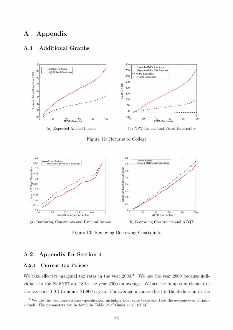
A Appendix

A.1 Additional Graphs

0 20 40 60 80 10020

30

40

50

60

70

80

90

100

Exp

ecte

d A

nn

ua

l In

co

me

in

1,0

00

AFQT−Percentile

College Graduate

High School Graduate

(a) Expected Annual Income

0 20 40 60 80 100−100

0

100

200

300

400

500

600

700

800

Do

llar

in 1

,00

0AFQT−Percentile

Expected NPV Earnings

Expected NPV Tax Payment

NPV Subsidies

Fiscal Externality

(b) NPV Income and Fiscal Externality

Figure 12: Returns to College

0 0.2 0.4 0.6 0.8 1Parental Income Percentile

0.1

0.15

0.2

0.25

0.3

0.35

0.4

0.45

0.5

0.55

0.6

Sh

are

of

Co

lleg

e G

rad

ua

tes

Current PoliciesRemoval of Borrowing Constraints

(a) Borrowing Constraints and Parental Income

0 20 40 60 80 100AFQT-Percentile

0

0.1

0.2

0.3

0.4

0.5

0.6

0.7

0.8

Sh

are

of

Co

lleg

e G

rad

ua

tes

Current PoliciesRemoval of Borrowing Constraints

(b) Borrowing Constraints and AFQT

Figure 13: Removing Borrowing Constraints

A.2 Appendix for Section 4

A.2.1 Current Tax Policies

We take effective marginal tax rates in the year 2000.21 We use the year 2000 because indi-

viduals in the NLSY97 are 18 in the year 2000 on average. We set the lump sum element of

the tax code T (0) to minus $1,800 a year. For average incomes this fits the deduction in the21We use the “Gouveia-Strauss”-specification including local sales taxes and take the average over all indi-

viduals. The parameters can be found in Table 12 of Guner et al. (2014).

34

US-tax code quite well.22 For low incomes this reflects that individuals might receive transfers

such as food stamps.23 We set the value of exogenous government spending to 11.2% of the

GDP, which is the value that leads to a balanced government budget. This value is a bit low,

but this should not be too surprising as we do not take into account corporate taxes or capital

income taxes and the population age structure.

A.2.2 Tuition Fees and Public Costs of Colleges

First, we categorize the following 4 regions:

• Northeast: CT, ME, MA, NH, NJ, NY, PA, RI, VT

• North Central: IL, IN, IA, KS, MI, MN, MO, NE, OH, ND, SD, WI

• South: AL, AR, DE, DC, FL, GA, KY, LA, MD, MS, NC, OK, SC, TN , TX, VA, WV

• West: AK, AZ, CA, CO, HI, ID, MT, NV, NM, OR, UT, WA, WY

We base the following calculations on numbers presented by Snyder and Hoffman (2001). Table

313 of this report contains average tuition fees for four-year public and private universities.

According to Table 173, 65% of all four-year college students went to public institutions,

whereas 35% went to private institutions. For each state we can therefore calculate the

average (weighted by the enrollment shares) tuition fee for a four-year college. We then use

these numbers to calculate the average for each of the four regions, where we weigh the different

states by their population size. We then arrive at numbers for yearly tuition & fees of $9,435

(North East), $7,646 (North Central), $6,414 (South) and $7,073 (West). For all individuals

in the data with missing information about their state of residence, we chose a country wide

population size weighted average of $7,434.

Tuition revenue of colleges typically only covers a certain share of their expenditure. Figures

18 and 19 in Snyder and Hoffman (2001) illustrate by which sources public and private colleges

finance cover their costs. Unfortunately no distinction between two and four-year colleges is

available. From Figures 18 and 19 we then infer how many dollars of public appropriations

are spent for each dollar of tuition. Many of these public appropriations are also used to

finance graduate students. It is unlikely that the marginal public appropriation for a bachelor

student therefore equals the average public appropriation at a college given that costs for22Guner et al. (2014) report a standard deduction of $7,350 for couples that file jointly. For an average tax

rate of 25% this deduction could be interpreted as a lump sum transfer of slightly more than $1,800.23The average amount of food stamps per eligible person was $72 per month in the

year 2000. Assuming a two person household gives roughly $1,800 per year. Source:http://www.fns.usda.gov/sites/default/files/pd/SNAPsummary.pdf

35

graduate students are higher. To solve this issue, we focus on institutions “that primarily

focus on undergraduate education” as defined in Table 345. Lastly, to avoid double counting

of grants and fee waivers, we exclude them from the calculation as we directly use the detailed

individual data about financial aid receipt from the NLSY (see Section A.2.5). Based on these

calculations we arrive at marginal public appropriations of $5,485 (Northeast), $4,514 (North

Central), $3,558 (South), $3,604 (West) and $4,157 (No information about region).

A.2.3 Details on Income Regressions

We first quickly explain the construction of the annuitized income variable. Assume that for

a high school graduate i, one observes yit for t = 1, ..., 48 – i.e. from 18 to 65. The discounted

present value of earnings (at age 18) is then given by∑48

t=0yit

(1+r)t−1 . Simply taking the average

over yt to obtain the relevant income for our model would be misleading since discounting is

not taken into account. Thus, we use annuitized income yi which is given by:

yi =

∑48t=1

yit(1+r)t−1∑48

t=11

(1+r)t−1

.

Everyone with less than 16 years of schooling is defined as a high school graduate.24 Ev-

eryone with 16 or more years of schooling is defined as a college graduate.

We run separate regressions, one for high school graduates and one for college graduates,

of the form:

ln yi = αce + βINe ln(AFQTi) + εincei , (12)

for e = hs, co. αce is a cohort-education fixed effect. We find that a one percent increase

in AFQT-test scores leads to a 1.88% increase in income for college graduates and 1.28%

increase in income for high school graduates, which reflects a complementarity between skills

and education.This procedure gives us the mean of log incomes as a function of an individual’s

AFQT-score and education level. Based on that, we then calculate the respective average

annual income over the life cycle for each AFQT-score and education level. We assume errors

are normally distributed, so income is distributed log-normally. To determine the second

moment of this log-normal distribution across education and innate ability levels, we use the

sample variances of the error terms from (12) for each education level.

For most individuals, we do not have information in every year. First of all, we never have

information after age 53. Second, since 1994 the survey is conducted biannually. Third, we

often have to deal with missing values. To resolve the first issue, we assume that incomes

are flat afterwards, which is roughly what one finds in data sets with information on earnings

over the whole life cycle. See, e.g., Figures 13 and 14 in Lee et al. (2014). Concerning the24Note that this definition also includes high school dropouts and individuals with community college

degrees. We also worked with different specifications but our main results were not significantly affected.

36

Table 2: Transfer Equation

Parental Income College Dependent Children

Coefficient .3136*** .5829*** -.0667**Standard Error (.0449) (.0563) (.0329 )

N=3,238. Robust standard errors. * p ≤ 0.10, ** p ≤ 0.05, *** p ≤ 0.01.

second issue, we take the average of the income in the year before and after. Concerning

the third issue, we proceed similarly but also take values that are two and three years away

if information for the year before and after is missing as well. All other years that are still

missing are then just not taken into account for calculating yi. Assume, e.g., that only income

at age 19, 33 and 46 were observable. Then we would calculate

yi =

yi19(1+r)

+ yi33(1+r)14

+ yi46(1+r)27

1(1+r)

+ 1(1+r)14

+ 1(1+r)27

.

All for all other monetary variables, incomes are measured in 2000 dollars.

Our estimates for the slopes are. βINC = 1.88 (0.186) and βINH = 1.28 (0.074). As described

in the main text, the second-moments of the log-normal parts are education dependent, so

that until 350k, ln y is normal with standard deviation σe. We directly take the estimates for

σe from the distribution of residuals from (12). The values are 0.6548 for college and 0.6631

for high-school.

A.2.4 Parental Transfers

In the NLSY97 we can observe the amount of transfers an individual obtained from its par-

ents as well as family income. We take the constructed variable for parental transfers from

Johnson (2013), who also takes into account the value of living at home as part of the parental

transfer, for those individuals who cohabitate with their parents. We take yearly averages of

those transfers for the ages 19-23. The sample average is $6,703. We estimate the following

equation:25

log(tri) = αtr + βtr1 log(Ii) + βtr2 coi + βtr3 depkidsi + εtri , (13)

where depkids is the number of dependent kids living in the household of the parents. The

coefficients are provided in Table 2. A 1% increase in parental income increases parental

transfers by 0.31% and college graduates receive transfers that are 79% (exp(.5829) − 1)

higher than for high school graduates. Note that this implies that the absolute increase of

parental transfers because of going to college is higher for high income kids. Johnson (2013)25We also estimated models with an interaction term between log parental income and college graduation.

The coefficient on the interaction term is statistically insignificant.

37

and Winter (2014) have argued that it is crucial to take this effect into account to explain the

large impact of parental income on college enrollment and completion.

Besides transfers that individuals receive during that time, they can also have some assets

when they decide to study. In the NLSY97, information is provided on individual net worth

at age 20. Certainly, this is not the best number for our purposes since it is highly influenced

by choices at ages 18 and 19. We nevertheless take this noisy measure into account because

it gives our quantitative model a better fit concerning the importance of parental income. To

measure how net wealth varies with parental income, we estimate the following regression:

wi = αw + βwIi + εwi . (14)

We find a gradient for parental income of .127 (0.02) and an intercept of $7,950 (1164). To

obtain the parental transfer for the model, we take the implied parental transfer from equation

(13) and adjust it by the implied level of wealth from equation (14) and thereby recalculate

the wealth into an annual transfer.

A.2.5 Estimation of Grant Receipt

In practice, grants and tuition subsidies are provided by a variety of different institutions. Pell

grants, for example, are provided by the federal government. In addition, there exist various

state and university programs. To make progress, similar to Johnson (2013) and others, we

go on to estimate grant receipt directly from the data.

Next, we estimate the amount of grants conditional on receiving grants:

gri = αgr + βgr1 Ii + βgr2 I2i + βgr3 blacki + βgr4 AFQTi + βgr5 depkidsi + εgri . (15)

Besides grant generosity being need-based (convexly decreasing) and in favor of blacks, gen-

erosity is also merit-based as βgr4 > 0 and increases with the number of other dependent

children (besides the considered student) in the family.

Table 3: OLS for Grants

Parental Income Parental Income2 Black AFQT Dependent Children

Coefficient -.0915*** 6.00e-07 *** 649.06** 23.90*** 224.69**Standard Error (0.0192) (1.83e-07) (296.03 ) ( 4.57) (99.11)

N=968. * p ≤ 0.10, ** p ≤ 0.05, *** p ≤ 0.01.

38

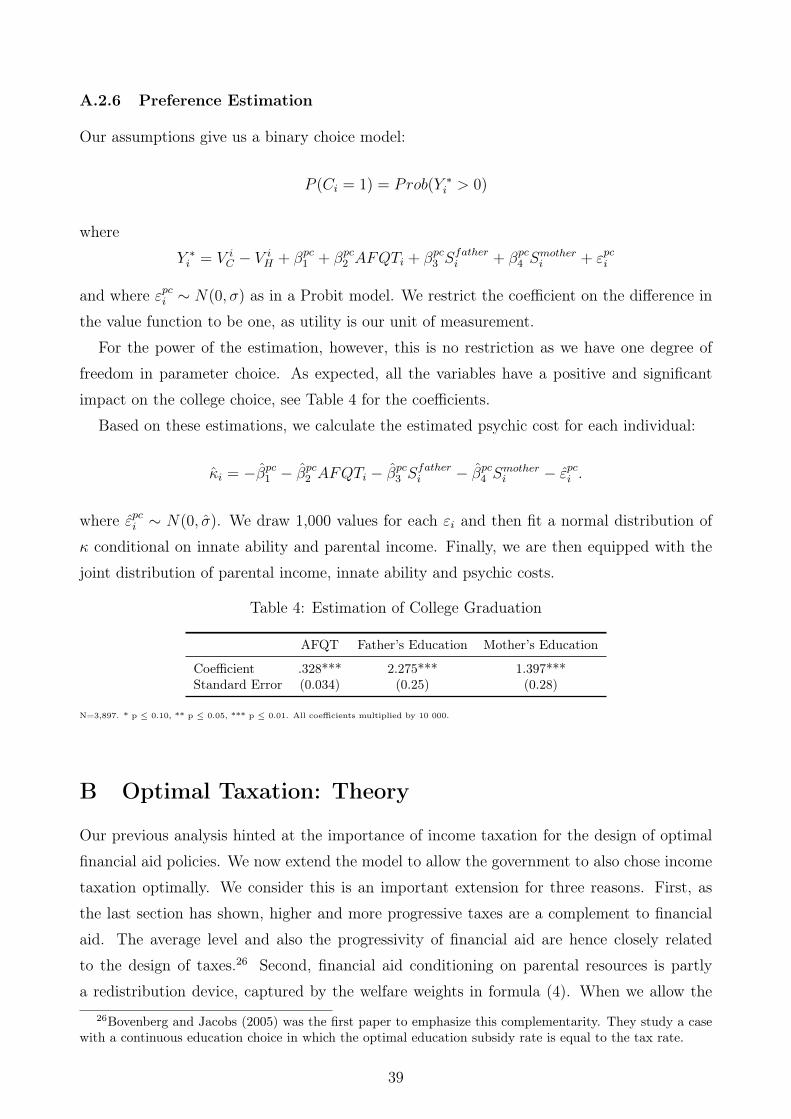
A.2.6 Preference Estimation

Our assumptions give us a binary choice model:

P (Ci = 1) = Prob(Y ∗i > 0)

where

Y ∗i = V iC − V i

H + βpc1 + βpc2 AFQTi + βpc3 Sfatheri + βpc4 S

motheri + εpci

and where εpci ∼ N(0, σ) as in a Probit model. We restrict the coefficient on the difference in

the value function to be one, as utility is our unit of measurement.

For the power of the estimation, however, this is no restriction as we have one degree of

freedom in parameter choice. As expected, all the variables have a positive and significant

impact on the college choice, see Table 4 for the coefficients.

Based on these estimations, we calculate the estimated psychic cost for each individual:

κi = −βpc1 − βpc2 AFQTi − β

pc3 S

fatheri − βpc4 S

motheri − εpci .

where εpci ∼ N(0, σ). We draw 1,000 values for each εi and then fit a normal distribution of

κ conditional on innate ability and parental income. Finally, we are then equipped with the

joint distribution of parental income, innate ability and psychic costs.

Table 4: Estimation of College Graduation

AFQT Father’s Education Mother’s Education

Coefficient .328*** 2.275*** 1.397***Standard Error (0.034) (0.25) (0.28)

N=3,897. * p ≤ 0.10, ** p ≤ 0.05, *** p ≤ 0.01. All coefficients multiplied by 10 000.

B Optimal Taxation: Theory

Our previous analysis hinted at the importance of income taxation for the design of optimal

financial aid policies. We now extend the model to allow the government to also chose income

taxation optimally. We consider this is an important extension for three reasons. First, as

the last section has shown, higher and more progressive taxes are a complement to financial

aid. The average level and also the progressivity of financial aid are hence closely related

to the design of taxes.26 Second, financial aid conditioning on parental resources is partly

a redistribution device, captured by the welfare weights in formula (4). When we allow the26Bovenberg and Jacobs (2005) was the first paper to emphasize this complementarity. They study a case

with a continuous education choice in which the optimal education subsidy rate is equal to the tax rate.

39

government to design the optimal non-linear tax system, we can analyze how much of the

progressivity of financial aid is driven by the desire to ex-ante redistribute. Finally, we can

theoretically and empirically analyze how taxes themselves may distort education decisions,

a channel analyzed in a prominent paper by Trostel (1993).

We build on the large literature following Mirrlees (1971) and the modern literature orig-

inating with Diamond (1998) and Saez (2001) expressing optimal tax schedules in terms of

observables (see Piketty and Saez (2013) for a review). Our model can stay very general in

terms of the underlying heterogeneity, while still preserving tractability.

The planner’s problem is the same as in (1) with the difference that the planner also opti-

mally chooses the income tax schedule T (·). Notice that the formula for optimal financial aid

policies is unaltered. We allow the tax function T (·) to be arbitrarily nonlinear in the spirit of

Mirrlees (1971). We restrict the tax function to be only a function of income and to be inde-

pendent of the education decision. This tax problem can either be tackled with a variational or

tax perturbation approach (Saez, 2001; Golosov et al., 2014; Jacquet and Lehmann, 2016) or

with a restricted mechanism design approach for nonlinear history-independent income taxes

that we explore in Findeisen and Sachs (2017).

Assumption Preferences UH(cHjw, y

Hjw;w, I,X

)and UW

(cWjw, y

Wjw;w, I,X

)imply no income

effects on labor supply.

As we show in Appendix B.1, the optimal marginal tax rate can be expressed as:

T ′(y(w∗))

1− T ′(y(w∗))=

1

εy(w∗),1−T ′×

(Haz(y(w∗)) (1−W(y(w∗))) +

∫R+ξ(I, y)∆T (I, y)dF (I)

h(y(w∗))y(w∗)

)(16)

where

Haz(y(w∗)) =

∫∞y(w∗)

h(y)dy

h(y(w∗))y(w∗)

and

h(y(w∗)) =βC2

∫R+

∫χ

1V C≥V Hk(I,X)gC(w∗|I,X)dIdX

+ βH∫R+

∫χ

1V H≤V Hk(I,X)gC(w∗|I,X)dIdX.

Note that Haz(y(w∗)) and h(y(w∗)) are basically the Hazard ratio (Saez, 2001) and the

density of income, only adjusted by period length. W(w) is a money metric average social

welfare weights of individuals with wage w. εy(w∗),1−T ′ is the local labor supply elasticity along

40

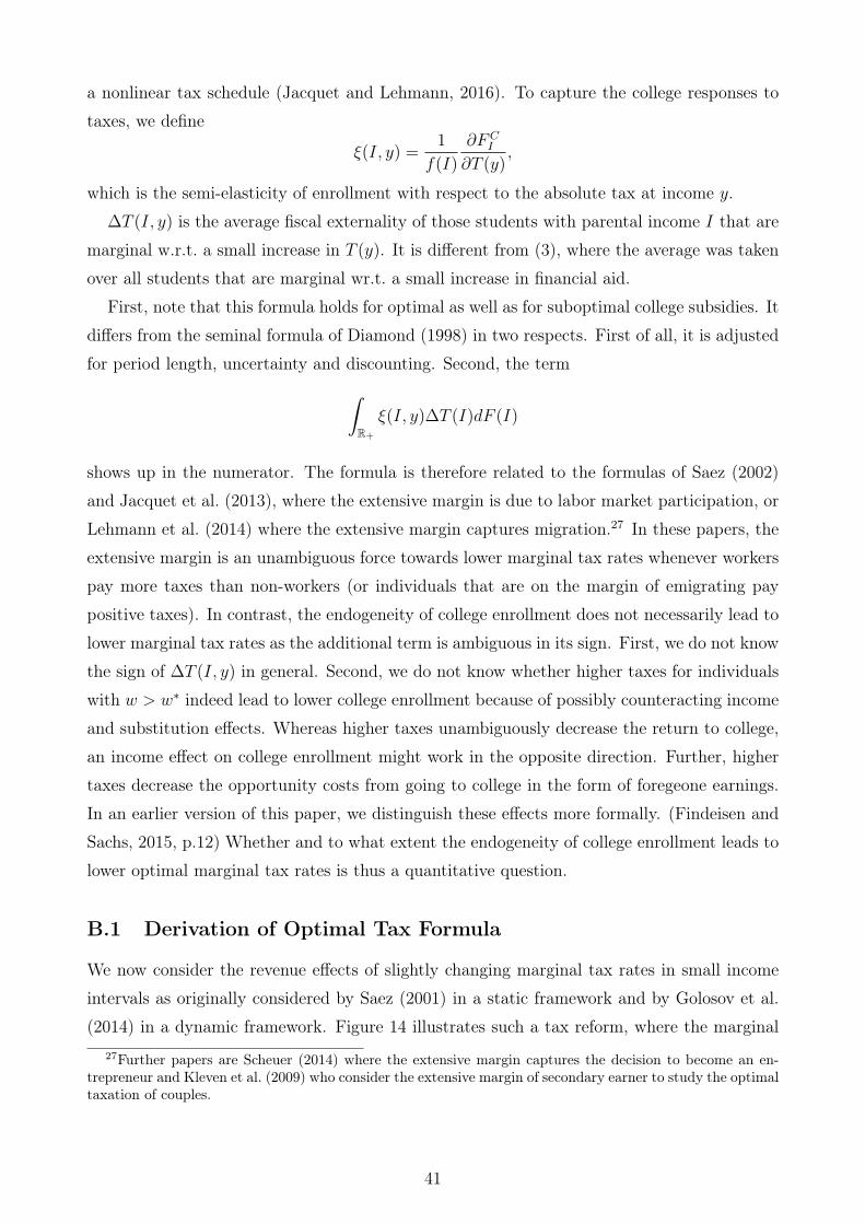
a nonlinear tax schedule (Jacquet and Lehmann, 2016). To capture the college responses to

taxes, we define

ξ(I, y) =1

f(I)

∂FCI

∂T (y),

which is the semi-elasticity of enrollment with respect to the absolute tax at income y.

∆T (I, y) is the average fiscal externality of those students with parental income I that are

marginal w.r.t. a small increase in T (y). It is different from (3), where the average was taken

over all students that are marginal wr.t. a small increase in financial aid.

First, note that this formula holds for optimal as well as for suboptimal college subsidies. It

differs from the seminal formula of Diamond (1998) in two respects. First of all, it is adjusted

for period length, uncertainty and discounting. Second, the term∫R+

ξ(I, y)∆T (I)dF (I)

shows up in the numerator. The formula is therefore related to the formulas of Saez (2002)

and Jacquet et al. (2013), where the extensive margin is due to labor market participation, or

Lehmann et al. (2014) where the extensive margin captures migration.27 In these papers, the

extensive margin is an unambiguous force towards lower marginal tax rates whenever workers

pay more taxes than non-workers (or individuals that are on the margin of emigrating pay

positive taxes). In contrast, the endogeneity of college enrollment does not necessarily lead to

lower marginal tax rates as the additional term is ambiguous in its sign. First, we do not know

the sign of ∆T (I, y) in general. Second, we do not know whether higher taxes for individuals

with w > w∗ indeed lead to lower college enrollment because of possibly counteracting income

and substitution effects. Whereas higher taxes unambiguously decrease the return to college,

an income effect on college enrollment might work in the opposite direction. Further, higher

taxes decrease the opportunity costs from going to college in the form of foregeone earnings.

In an earlier version of this paper, we distinguish these effects more formally. (Findeisen and

Sachs, 2015, p.12) Whether and to what extent the endogeneity of college enrollment leads to

lower optimal marginal tax rates is thus a quantitative question.

B.1 Derivation of Optimal Tax Formula

We now consider the revenue effects of slightly changing marginal tax rates in small income

intervals as originally considered by Saez (2001) in a static framework and by Golosov et al.

(2014) in a dynamic framework. Figure 14 illustrates such a tax reform, where the marginal27Further papers are Scheuer (2014) where the extensive margin captures the decision to become an en-

trepreneur and Kleven et al. (2009) who consider the extensive margin of secondary earner to study the optimaltaxation of couples.

41

tax is increased by an infinitesimal amount dT ′ in an income interval of infinitesimal length

[y(w∗), y(w∗) + dy].

Income

Taxes

Increase of Marginal

Increase of Absolute Tax Payment

y(w*)

= dT' dy

=dy

Tax Rate by dT'

Figure 14: Tax Reform

As a consequence of this reform, all individuals with y > y(w∗) (and therefore w > w∗) face

an increase of the absolute tax level of dT ′dy. The tax reform therefore induces a mechanical

increase in tax revenue of

M(y(w∗)) = dT ′dy

∫ ∞y(w∗)

.h(y)dy

where

h(y) =βC2

∫R+

∫χ

1V C≥V Hk(I,X)gC(w(y)|I,X)dIdX

+ βH∫R+

∫χ

1V C≤V Hk(I,X)gC(w(y)|I,X)dIdX.

The increase in taxes for individuals with w > w∗ also changes incentives for enrollment.

In fact, graduation will increase by:

CG(y(w∗)) = dT ′dy

∫ ∞y(w∗)

∫R+

ξ(I, y)dF (I)dy.

where

ξ(I, y) =1

f(I)

∂FCI

∂T (y),

is the semi-elasticity of college graduation with respect to an increase in T (y). This increase

in graduation has no first-order effect on welfare as these marginal individuals are just indif-

ferent between obtaining a college degree or not. It has a first-order effect on the government

budget which is given by:

42

CG(y(w∗)) = dT ′dy

∫ ∞y(w∗)

∫R+

ξ(I, y)∆T (I, y)dF (I)dy.

∆T (I, y) is the average fiscal externality of those students with parental income y∗ that are

marginal w.r.t. a small increase in T (y). It is different from (3), where the average was taken

overall that are marginal wr.t. a small increase in financial aid.

In addition, an increase in the marginal tax rate also affects labor supply behavior for

individuals within the interval [y(w∗), y(w∗)+dy]. Individuals within this infinitesimal interval

change their labor supply by

∂y(w∗)

∂T ′dT ′ = −εy,1−T ′

y

1− T ′dT ′. (17)

Whereas this change in labor supply has no first-order effect on welfare via individual utilities

by the envelope theorem, it has an effect on tax revenue. The mass of these individuals is

then given by

h(y(w∗))dy

The overall impact on public funds (adjusted by period length and discounting) is therefore

given by

LS(y(w∗)) = −εy(w∗),1−T ′y(w∗)

1− T ′dT ′h(y(w∗))dy.

The overall impact on welfare of the considered tax reform is thus given by

Γ(y(w∗)) = M(y(w∗)) + CG(y(w∗)) + LS(y(w∗)). (18)

For an optimal tax system these effects have to add up to zero. Γ(y(w∗)) = 0 yields the

optimal tax formula (16).

43

References

Abbott, B., G. Gallipoli, C. Meghir, and G. L. Violante (2016): “Education Policy

and Intergenerational Transfers in Equilibrium,” Cowles Foundation Discussion Paper No.

1887R.

Alsalam, N. (2013): “The Federal Pell Grant program: Recent growth and policy options,”

Washington, DC: Congressional Budget Office.

Altonji, J., P. Bharadwaj, and F. Lange (2012): “Changes in the characteristics of

American youth: Implications for adult outcomes,” Journal of Labor Economics, 30, 783–

828.

Altonji, J. and T. Dunn (1996): “The Effects of Family Characteristics on the Return to

Education,” The Review of Economics and Statistics, 78, 692–704.

Angrist, J., D. Autor, S. Hudson, and A. Pallais (2015): “Leveling Up: Early Results

from a Randomized Evaluation of Post-Secondary Aid,” Working Paper.

Bagnoli, M. and T. Bergstrom (2005): “Log-concave probability and its applications,”

Economic theory, 26, 445–469.

Baum, S., J. Ma, and K. Payea (2013): “Education Pays, 2013: The Benefits of Higher

Education for Individuals and Society. Trends in Higher Education Series.” College Board.

Belley, P. and L. Lochner (2007): “The changing role of family income and ability in

determining educational achievement,” Journal of Human capital, 1, 37–89.

Best, M. and H. Kleven (2013): “Optimal Income Taxation with Career Effects of Work

Effort,” Working Paper, London School of Economics.

Bettinger, E. (2004): “How financial aid affects persistence,” in College choices: The eco-

nomics of where to go, when to go, and how to pay for it, University of Chicago Press,

207–238.

Bohacek, R. and M. Kapicka (2008): “Optimal Human Capital Policies,” Journal of

Monetary Economics, 55, 1–16.

Bovenberg, L. and B. Jacobs (2005): “Redistribution and Education Subsidies are

Siamese Twins,” Journal of Public Economics, 89, 2005–2035.

Card, D. (1999): “The causal effect of education on earnings,” Handbook of Labor Economics,

3, 1801–1863.

44

Carneiro, P. and J. Heckman (2003): “Human Capital Policy,” IZA Discussion Paper

No. 821.

Carroll, S. J. and E. Erkut (2009): The benefits to taxpayers from increases in students’

educational attainment, vol. 686, Rand Corporation.

Castleman, B. L. and B. T. Long (2016): “Looking beyond enrollment: The causal

effect of need-based grants on college access, persistence, and graduation,” Journal of Labor

Economics, 34, 1023–1073.

Chetty, R. (2009): “Sufficient Statistics for Welfare Analysis: A Bridge Between Structural

and Reduced-Form Methods,” Annu. Rev. Econ., 1, 451–488.

Chetty, R., J. N. Friedman, and J. E. Rockoff (2014): “Measuring the Impacts of

Teachers II: Teacher Value-Added and Student Outcomes in Adulthood,” American Eco-

nomic Review, 104, 2633–79.

Chetty, R., A. Guren, D. Manoli, and A. Weber (2011): “Are Micro and Macro

Labor Supply Elasticities Consistent? A Review of Evidence on the Intensive and Extensive

Margins,” American Economic Review Papers and Proceedings, 101, 471–475.

College Board (2015): “Trends in Student Aid 2015,” College Board.

Cunha, F., J. Heckman, and S. Navarro (2005): “Separating uncertainty from hetero-

geneity in life cycle earnings,” Oxford Economic Papers, 57, 191–261.

Cunha, F., F. Karahan, and I. Soares (2011): “Returns to skills and the college pre-

mium,” Journal of Money, Credit and Banking, 43, 39–86.

Deming, D. and S. Dynarski (2009): “Into college, out of poverty? Policies to increase the

postsecondary attainment of the poor,” NBER Working Paper 15387.

Diamond, P. (1980): “Income Taxation with Fixed Hours of Work,” Journal of Public Eco-

nomics, 13, 101–110.

Diamond, P. A. and E. Saez (2011): “The Case for a Progressive Tax: From Basic Research

to Policy Recommendations,” Journal of Economic Perspectives, 25, 165–190.

Dynarski, S. M. (2003): “Does Aid Matter? Measuring the Effect of Student Aid on College

Attendance and Completion,” The American Economic Review, 93, 279–288.

Findeisen, S. and D. Sachs (2015): “Designing Efficient College and Tax Policies,” Working

Paper.

45

——— (2016): “Education and Optimal Dynamic Taxation: The Role of Income-Contingent

Student Loans,” Journal of Public Economics, 138, 1–21.

——— (2017): “Redistribution and Insurance with Simple Tax Instruments,” Journal of Public

Economics, 146, 58–78.

Gelber, A. and M. Weinzierl (2016): “Equalizing Outcomes vs. Equalizing Opportunities:

Optimal Taxation when Children’s Abilities Depend on Parents’ Resources,” National Tax

Journal, 69, 11–40.

Goldin, C. D. and L. F. Katz (2009): The race between education and technology, Harvard

University Press.

Golosov, M., A. Tsyvinski, and N. Werquin (2014): “A Variational Approach to the

Analysis of Tax Systems,” Working Paper.

Guner, N., R. Kaygusuz, and G. Ventura (2014): “Income taxation of US households:

Facts and parametric estimates,” Review of Economic Dynamics, 17, 559–581.

Heathcote, J., K. Storesletten, and G. L. Violante (2016): “Optimal tax progres-

sivity: An analytical framework,” Quarterly Journal of Economics (forthcoming).

Heckman, J. J., L. J. Lochner, and P. E. Todd (2006): “Earnings functions, rates of

return and treatment effects: The Mincer equation and beyond,” Handbook of the Economics

of Education, 1, 307–458.

Hendren, N. (2014): “The inequality deflator: Interpersonal comparisons without a social

welfare function,” NBER Working Paper 20351.

——— (2015): “The Policy Elasticity,” in Tax Policy and the Economy, Volume 30, University

of Chicago Press.

Hilger, N. G. (2016): “Parental Job Loss and Children’s Long-Term Outcomes: Evidence

from 7 Million Fathers’ Layoffs,” American Economic Journal: Applied Economics, 8, 247–

283.

Imbens, G. W., D. B. Rubin, and B. I. Sacerdote (2001): “Estimating the effect of

unearned income on labor earnings, savings, and consumption: Evidence from a survey of

lottery players,” American Economic Review, 778–794.

Jacquet, L. and E. Lehmann (2016): “Optimal Taxation with Heterogeneous Skills and

Elasticities: Structural and Sufficient Statistics Approaches,” THEMA Working Paper 2016-

04.

46

Jacquet, L., E. Lehmann, and B. Van der Linden (2013): “The Optimal Marginal Tax

Rates with both Extensive and Intensive Responses,” Journal of Economic Theory, 148,

1770–1805.

Johnson, M. T. (2013): “Borrowing Constraints, College Enrollment, and Delayed Entry,”

Journal of Labor Economics, 31, 669–725.

Kane, T. J. (2006): “Public intervention in post-secondary education,” Handbook of the

Economics of Education, 2, 1369–1401.

Kleven, H., C. Kreiner, and E. Saez (2009): “The Optimal Income Taxation of Couples,”

Econometrica, 77, 537–560.

Kline, P. and C. R. Walters (2016): “Evaluating public programs with close substitutes:

The case of Head Start,” The Quarterly Journal of Economics, 131, 1795–1848.

Koeniger, W. and J. Prat (2017): “Human Capital and Optimal Redistribution,” Working

Paper.

Krueger, D. and A. Ludwig (2013): “Optimal Progressive Labor Income Taxation and

Education Subsidies when Education Decisions and Intergenerational Transfers are Endoge-

nous,” American Economic Review Papers & Proceedings, 103, 496–501.

——— (2016): “On the optimal provision of social insurance: Progressive taxation versus

education subsidies in general equilibrium,” Journal of Monetary Economics, 77, 72–98.

Laun, T. and J. Wallenius (2016): “Social insurance and retirement: a cross-country

perspective,” Review of Economic Dynamics, 22, 72–92.

Lawson, N. (2016): “Liquidity Constraints, Fiscal Externalities and Optimal Tuition Subsi-

dies,” American Economic Journal: Economic Policy (forthcoming).

Lee, D., S. Y. Lee, and Y. Shin (2014): “The Option Value of Human Capital,” Working

Paper.

Lehmann, E., L. Simula, and A. Trannoy (2014): “Tax me if you can! Optimal nonlinear

income tax between competing governments,” The Quarterly Journal of Economics, 129,

1995–2030.

Navarro, S. (2011): “Using observed choices to infer agent’s information: Reconsidering the

importance of borrowing constraints, uncertainty and preferences in college attendance,”

CIBC Working Paper.

47

OECD (2014): “Education at a Glance 2014: OECD Indicators,” URL:

http://dx.doi.org/10.1787/eag-2014-en.

Oreopoulos, P. and U. Petronijevic (2013): “Making college worth it: A review of

research on the returns to higher education,” NBER Working Paper 19053.

Piketty, T. and E. Saez (2013): “Optimal labor income taxation,” Handbook of Public

Economics, Vol 5.

Saez, E. (2001): “Using Elasticities to Derive Optimal Income Tax Rates,” The Review of

Economic Studies, 68, 205–229.

——— (2002): “Optimal Income Transfer Programs: Intensive versus Extensive Labor Supply

Responses,” Quarterly Journal of Economics, 117, 1039–1073.

Saez, E. and S. Stantcheva (2016): “Generalized Social Marginal Welfare Weights for

Optimal Tax Theory,” American Economic Review, 106, 24–45.

Scheuer, F. (2014): “Entrepreneurial Taxation with Endogenous Entry,” American Eco-

nomic Journal: Economic Policy, 6, 126–163.

Shapiro, D., A. Dundar, J. Chen, M. Ziskin, E. Park, V. Torres, and Y.-C. Chiang

(2012): “Completing College: A National View of Student Attainment Rates. Signature

[TM] Report 4.” National Student Clearinghouse.

Snyder, T. D. and S. A. Dillow (2013): Digest of education statistics 2012, National

Center for Education Statistics.

Snyder, T. D. and C. M. Hoffman (2001): Digest of education statistics 2000, National

Center for Education Statistics.

Stantcheva, S. (2015): “Optimal Income, Education, and Bequest Taxes in an Intergener-

ational Model,” NBER Working Paper No. 21177.

——— (2016): “Optimal Taxation and Human Capital Policies Over the Lifecycle,” Journal

of Political Economy (forthcoming).

Trostel, P. A. (1993): “The effect of taxation on human capital,” Journal of Political

Economy, 327–350.

Winter, C. (2014): “Accounting for the Changing Role of Family Income in Determining

College Entry,” Scandinavian Journal of Economics, 116, 909–963.

Zimmerman, S. (2014): “The returns to college admission for academically marginal stu-

dents,” Journal of Labor Economics, 32, 711–754.

48