Optimal queue-size scaling in switched networks · 4 D. SHAH, N. S. WALTON AND Y. ZHONG ﬁrst describe the policy for single-hop switched networks, and state our main result, Theorem

arX

iv:1

110.

4697

v3 [

mat

h.PR

] 3

Sep

201

4

The Annals of Applied Probability

2014, Vol. 24, No. 6, 2207–2245DOI: 10.1214/13-AAP970c© Institute of Mathematical Statistics, 2014

OPTIMAL QUEUE-SIZE SCALING IN SWITCHED NETWORKS

By D. Shah1, N. S. Walton and Y. Zhong1

Massachusetts Institute of Technology, University of Amsterdamand Columbia University

We consider a switched (queuing) network in which there areconstraints on which queues may be served simultaneously; such net-works have been used to effectively model input-queued switches andwireless networks. The scheduling policy for such a network specifieswhich queues to serve at any point in time, based on the currentstate or past history of the system. In the main result of this pa-per, we provide a new class of online scheduling policies that achieveoptimal queue-size scaling for a class of switched networks includ-ing input-queued switches. In particular, it establishes the validityof a conjecture (documented in Shah, Tsitsiklis and Zhong [Queue-ing Syst. 68 (2011) 375–384]) about optimal queue-size scaling forinput-queued switches.

1. Introduction. A switched network consists of a collection of, say,N queues, operating in discrete time. At each time slot, queues are offeredservice according to a service schedule chosen from a specified finite set,denoted by S . The rule for choosing a schedule from S at each time slotis called the scheduling policy. New work may arrive to each queue at eachtime slot exogenously and work served from a queue may join another queueor leave the network. We shall restrict our attention, however, to the casewhere work arrives in the form of unit-sized packets, and once it is servedfrom a queue, it leaves the network, that is, the network is single-hop.

Switched networks are special cases of what Harrison [15, 16] calls “stochas-tic processing networks.” Switched networks are general enough to model a

Received October 2011; revised December 2012.1Supported by NSF TF collaborative project and NSF CNS CAREER project. When

this work was performed, the third author was affiliated with the Laboratory for Informa-tion and Decision Systems as well as the Operations Research Center at MIT. The thirdauthor is now affiliated with the Department of Industrial Engineering and OperationsResearch at Columbia University.

AMS 2000 subject classifications. 60K25, 60K30, 90B36.Key words and phrases. Switched network, maximum weight scheduling, fluid models,

state space collapse, heavy traffic, diffusion approximation.

This is an electronic reprint of the original article published by theInstitute of Mathematical Statistics in The Annals of Applied Probability,2014, Vol. 24, No. 6, 2207–2245. This reprint differs from the original inpagination and typographic detail.

1

http://arxiv.org/abs/1110.4697v3

http://www.imstat.org/aap/

http://dx.doi.org/10.1214/13-AAP970

http://www.imstat.org

http://www.ams.org/msc/

http://www.imstat.org

http://www.imstat.org/aap/

http://dx.doi.org/10.1214/13-AAP970

2 D. SHAH, N. S. WALTON AND Y. ZHONG

variety of interesting applications. For example, they have been used to ef-fectively model input-queued switches, the devices at the heart of high-endInternet routers, whose underlying silicon architecture imposes constraintson which traffic streams can be transmitted simultaneously [8]. They havealso been used to model multihop wireless networks in which interferencelimits the amount of service that can be given to each host [35]. Finally,they can be instrumental in finding the right operational point in a datacenter [31].

In this paper, we consider online scheduling policies, that is, policies thatonly utilize historical information (i.e., past arrivals and scheduling deci-sions). The performance objective of interest is the total queue size or totalnumber of packets waiting to be served in the network on average (appro-priately defined). The questions that we wish to answer are: (a) what isthe minimal value of the performance objective among the class of onlinescheduling policies, and (b) how does it depend on the network structure,S , as well as the effective load.

Consider a work-conservingM/D/1 queue with a unit-rate server in whichunit-sized packets arrive as a Poisson process with rate ρ ∈ (0,1). Then, thelong-run average queue-size scales2 as 1/(1− ρ). Such scaling dependence ofthe average queue size on 1/(1 − ρ) (or the inverse of the gap, 1− ρ, fromthe load to the capacity) is a universally observed behavior in a large classof queuing networks. In a switched network, the scaling of the average to-tal queue size ought to depend on the number of queues, N . For example,consider N parallel M/D/1 queues as described above. Clearly, the aver-age total queue size will scale as N/(1− ρ). On the other hand, consider avariation where all of these queues pool their resources into a single serverthat works N times faster. Equivalently, by a time change, let each of theN queues receive packets as an independent Poisson process of rate ρ/N ,and each time a common unit-rate server serves a packet from one of thenonempty queues. Then, the average total queue-size scales as 1/(1 − ρ).Indeed, these are instances of switched networks that differ in their schedul-ing set S , which leads to different queue-size scalings. Therefore, a naturalquestion is the determination of queue-size scaling in terms of S and (1−ρ),where ρ is the effective load. In the context of an n-port input-queued switchwith N = n2 queues, the optimal scaling of average total queue size has beenconjectured to be n/(1− ρ), that is,

√N/(1− ρ) [29].

As the main result of this paper, we propose a new online schedulingpolicy for any single-hop switched network. This policy effectively emulatesan insensitive bandwidth sharing network with a product-form stationary

2In this paper, by scaling of quantity we mean its dependence (ignoring universalconstants) on 1

1−ρand/or the number of queues, N , as these quantities become large.

Of particular interest is the scaling of ρ→ 1 and N →∞, in that order.

OPTIMAL SCHEDULING 3

distribution with each component of this product-form behaving like anM/M/1 queue. This crisp description of stationary distribution allows us toobtain precise bounds on the average queue sizes under this policy. This leadsto establishing, as a corollary of our result, the validity of a conjecture statedin [29] for input-queued switches. In general, it provides explicit bounds onthe average total queue size for any switched network. Furthermore, dueto the explicit bound on the stationary distribution of queue sizes underour policy, we are able to establish a form of large-deviations optimality ofthe policy for a large class of single-hop switched networks, including theinput-queued switches, and the independent-set model of wireless networks,when the underlying interference graph is bipartite, for example, and moregenerally, perfect.

The conjecture from [29] that we settle in this paper, states that in theheavy-traffic regime (i.e., ρ→ 1), the optimal average total queue-size scalesas

√N/(1− ρ). The validity of this conjecture is a significant improvement

over the best-known bounds of O(N/(1− ρ)) (due to the moment bounds of[24] for the maximum weight policy) or O(

√N logN/(1− ρ)2) (obtained by

using a batching policy [25]).Our analysis consists of two principal components. First, we propose and

analyze a scheduling mechanism that is able to emulate, in discrete time,any continuous-time bandwidth allocation within a bounded degree of error.This scheduler maintains a continuous-time queuing process and tracks itsown queue size process. If, valued under a certain decomposition, the gapbetween the idealized continuous-time process and the real queuing processbecomes too large, then an appropriate schedule is allocated. Second, weimplement specific bandwidth allocation named the store-and-forward al-location policy (SFA). This policy was first considered by Massoulie, andwas consequently discussed in the thesis of Proutiere [26], Section 3.4. Itwas shown to be insensitive with respect to phase-type service distributionsin works by Bonald and Proutiere [3, 4]. The insensitivity of this policyfor general service distributions was established by Zachary [41]. The store-and-forward policy is closely related to the classical product-form multi-classqueuing network, which have highly desirable queue-size scalings. By emu-lating these queuing networks, we are able to translate results which renderoptimal queue-size bounds for a switched network. An interested reader isreferred to [38] and [20] for an in-depth discussion on the relation betweenthis policy, the proportionally fair allocation, and multi-class queuing net-works.

1.1. Organization. In Section 2, we specify a stochastic switched networkmodel. In Section 3, we discuss related works. Section 4 details the necessarybackground on the insensitive store-and-forward bandwidth allocation (SFA)policy. The main result of the paper is presented and proved in Section 5. We


first describe the policy for single-hop switched networks, and state our mainresult, Theorem 5.2. This is followed by a discussion of the optimality of thepolicy. We then provide a proof of Theorem 5.2. A discussion of directionsfor future work is provided in Section 6.

Notation. Let N be the set of natural numbers {1,2, . . .}, let Z+ = {0,1,2, . . .}, let R be the set of real numbers and let R+ = {x ∈ R :x ≥ 0}. LetI[A] be the indicator function of an event A, Let x∧ y =min(x, y), x∨ y =max(x, y) and [x]+ = x ∨ 0. When x is a vector, the maximum is takencomponentwise.

We will reserve bold letters for vectors in RN , where N is the number

of queues. For example, x = [xn]1≤n≤N . Superscripts on vectors are usedto denote labels, not exponents, except where otherwise noted; thus, forexample, (x0,x1,x2) refers to three arbitrary vectors. Let 0 be the vector ofall 0s and 1 the vector of all 1s. The vector ei is the ith unit vector, withall components being 0 but the ith component equal to 1. We use the norm|x|=maxn |xn|. For vectors u and v, we let u · v=

∑Nn=1 unvn. Let A

T bethe transpose of matrix A. For a set S ⊂R

N , denote its convex hull by 〈S〉.For n ∈N, let n! =

∏nℓ=1 ℓ be the factorial of n, and by convention, 0! = 1.

2. Switched network model. We now introduce the switched networkmodel. Section 2.1 describes the general system model, Section 2.2 lists theprobabilistic assumptions about the arrival process and Section 2.3 intro-duces some useful definitions.

2.1. Queueing dynamics. Consider a collection of N queues. Let time bediscrete, and indexed by τ ∈ {0,1, . . .}. Let Qi(τ) be the amount of workin queue i ∈ {1, . . . ,N} at time slot τ . Following our general notation forvectors, we write Q(τ) for [Qi(τ)]1≤i≤N . The initial queue sizes are Q(0).Let Ai(τ) be the total amount of work arriving to queue i, and Bi(τ) be thecumulative potential service to queue n, up to time τ , with A(0) =B(0) = 0.

We first define the queuing dynamics for a single-hop switched network.Defining dA(τ) =A(τ +1)−A(τ) and dB(τ) =B(τ +1)−B(τ), the basicLindley recursion that we will consider is

Q(τ + 1) = [Q(τ)− dB(τ)]+ + dA(τ),(1)

where the operation [·]+ is applied componentwise. The fundamental switchednetwork constraint is that there is some finite set S ⊂R

N+ such that

dB(τ) ∈ S for all τ.(2)

For the purpose of this work, we shall focus on S ⊂ {0,1}N . We will refer toσ ∈ S as a schedule and S as the set of allowed schedules. In the applications


in this paper, the schedule is chosen based on current queue sizes, which iswhy it is natural to write the basic Lindley recursion as (1) rather than themore standard [Q(τ) + dA(τ)− dB(τ)]+.

For the analysis in this paper, it is useful to keep track of two otherquantities. Let Zi(τ) be the cumulative amount of idling at queue n, definedby Z(0) = 0 and

dZ(τ) = [dB(τ)−Q(τ)]+,(3)

where dZ(τ) = Z(τ +1)−Z(τ). Then, (1) can be rewritten as

Q(τ) =Q(0) +A(τ)−B(τ) +Z(τ).(4)

Also, let Sσ(τ) be the cumulative amount of time that is spent on usingschedule σ up to time τ , so that

B(τ) =∑

σ∈S

Sσ(τ)σ.(5)

A policy that decides which schedule to choose at each time slot τ ∈ Z+

is called a scheduling policy. In this paper, we will be interested in onlinescheduling policies. That is, the scheduling decision at time τ will be basedon historical information, that is, the cumulative arrival process A(·) tilltime τ .

2.2. Stochastic model. We shall assume that the exogenous arrival pro-cess for each queue is independent and Poisson. Specifically, unit-sized pack-ets arrive to queue i as a Poisson process of rate λi. Let λ= [λi]

Ni=1 denote

the vector of all arrival rates. The results presented in this paper extend tomore general arrival process with i.i.d. interarrival times with finite means,using a Poissonization trick. We discuss this extension in Section 6.

2.3. Useful quantities. We shall assume that the scheduling constraintset S is monotone. This is captured in the following assumption.

Assumption 2.1 (Monotonicity). If S contains a schedule, then S alsocontains all of its sub-schedules. Formally, for any σ ∈ S , if σ′ ∈ {0,1}N andσ′ ≤ σ componentwise, then σ′ ∈ S .

Without loss of generality, we will assume that each unit vector ei belongsto S . Next, we define some quantities that will be useful in the remainderof the paper.

Definition 2.2 (Admissible region). Let S ⊂ {0,1}N be the set of al-lowed schedules. Let 〈S〉 be the convex hull of S , that is,

〈S〉={∑

σ∈S

ασσ :∑

σ∈S

ασ = 1 and ασ ≥ 0, for all σ

}.


Define the admissible region C to be

C = {λ ∈RN+ :λ≤ σ componentwise, for some σ ∈ 〈S〉}.

Note that under Assumption 2.1, the capacity region C and the convexhull 〈S〉 of S coincide.

Given that 〈S〉 is a polytope contained in [0,1]N , there exists an integerJ ≥ 1, a matrix R ∈R

J×N+ and a vector C ∈R

J+ such that

〈S〉= {x ∈ [0,1]N :Rx≤C}.(6)

We call J the rank of 〈S〉 in the representation (6). When it is clear fromthe context, we simply call J the rank of 〈S〉. Note that this rank may bedifferent from the rank of matrix R. Our results will exploit the fact thatthe rank J may be an order of magnitude smaller than N .

Definition 2.3 (Static planning problems and load). Define the staticplanning optimization problem PRIMAL(λ) for λ ∈R

N+ to be

minimize∑

σ∈S

ασ,(7)

subject to λ≤∑

σ∈S

ασσ,(8)

ασ ∈R+ for all σ ∈ S.(9)

Define the induced load by λ, denoted by ρ(λ), as the value of the optimiza-tion problem PRIMAL(λ).

Note that λ is admissible if and only if ρ(λ)≤ 1. It also follows immedi-ately from Definition 2.3 that

ρ(λ) = inf{γ ≥ 0 :Rλ≤ γC},(10)

and λ is admissible if and only if Rλ≤C, componentwise.In the sequel, we will often consider the quantities ρj =

∑iRjiλi/Cj , for

j ∈ {1,2, . . . , J}, which can be interpreted as loads on individual “resources”of the system (this interpretation will be made precise in Section 4). Theyare closely related to the system load ρ(λ). We formalize this relation in thefollowing lemma, whose proof is straightforward and omitted.

Lemma 2.4. Consider a nonnegative matrix R ∈ RJ×N+ and a vector

C ∈RJ with Cj > 0 for all j. For a nonnegative vector λ ∈R

N+ , define ρ(λ)

by (10) and ρj = (∑

iRjiλi)/Cj . Then ρ(λ) = maxj ρj .

The following is a simple and useful property of ρ(·): for any a,b∈RN+ ,

ρ(a+ b)≤ ρ(a) + ρ(b).(11)


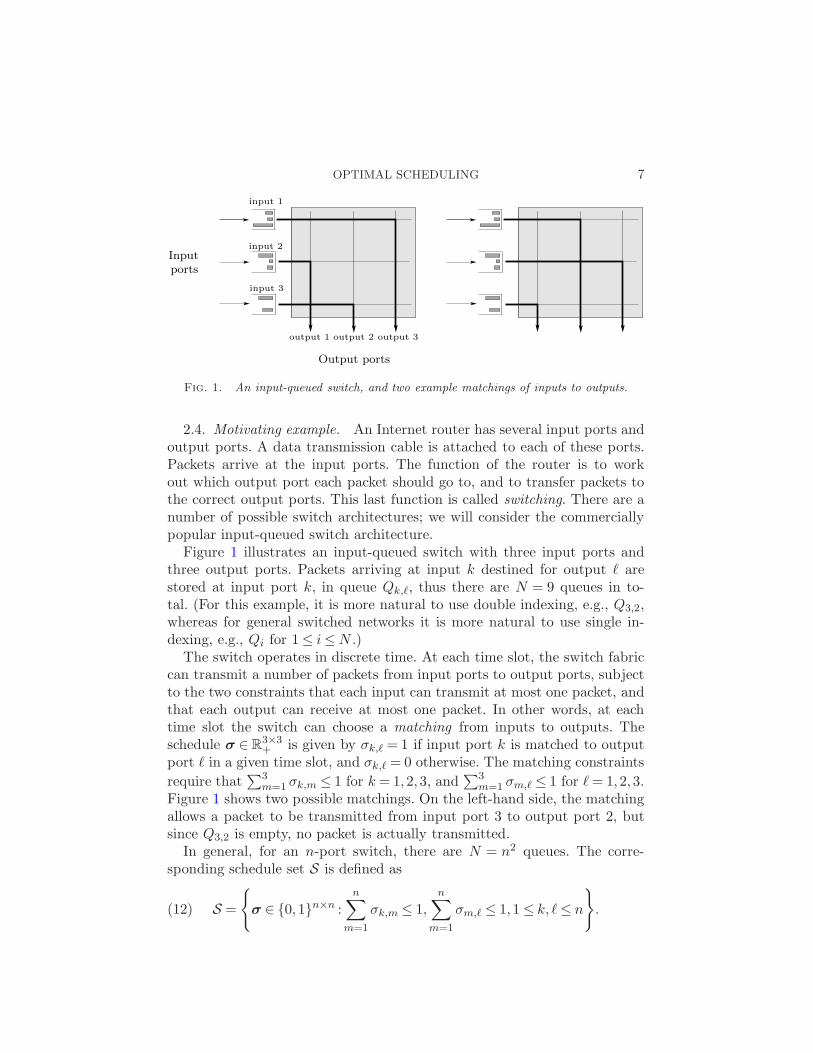
Fig. 1. An input-queued switch, and two example matchings of inputs to outputs.

2.4. Motivating example. An Internet router has several input ports andoutput ports. A data transmission cable is attached to each of these ports.Packets arrive at the input ports. The function of the router is to workout which output port each packet should go to, and to transfer packets tothe correct output ports. This last function is called switching. There are anumber of possible switch architectures; we will consider the commerciallypopular input-queued switch architecture.

Figure 1 illustrates an input-queued switch with three input ports andthree output ports. Packets arriving at input k destined for output ℓ arestored at input port k, in queue Qk,ℓ, thus there are N = 9 queues in to-tal. (For this example, it is more natural to use double indexing, e.g., Q3,2,whereas for general switched networks it is more natural to use single in-dexing, e.g., Qi for 1≤ i≤N .)

The switch operates in discrete time. At each time slot, the switch fabriccan transmit a number of packets from input ports to output ports, subjectto the two constraints that each input can transmit at most one packet, andthat each output can receive at most one packet. In other words, at eachtime slot the switch can choose a matching from inputs to outputs. Theschedule σ ∈R

3×3+ is given by σk,ℓ = 1 if input port k is matched to output

port ℓ in a given time slot, and σk,ℓ = 0 otherwise. The matching constraints

require that∑3

m=1 σk,m ≤ 1 for k = 1,2,3, and∑3

m=1 σm,ℓ ≤ 1 for ℓ= 1,2,3.Figure 1 shows two possible matchings. On the left-hand side, the matchingallows a packet to be transmitted from input port 3 to output port 2, butsince Q3,2 is empty, no packet is actually transmitted.

In general, for an n-port switch, there are N = n2 queues. The corre-sponding schedule set S is defined as

S =

{σ ∈ {0,1}n×n :

n∑

m=1

σk,m ≤ 1,n∑

m=1

σm,ℓ ≤ 1,1≤ k, ℓ≤ n

}.(12)


It can be checked that S is monotone. Furthermore, due to Birkhoff–vonNeumann theorem, [2, 37], the convex hull of S is given by

〈S〉={x ∈ [0,1]n×n :

n∑

m=1

xk,m ≤ 1,n∑

m=1

xm,ℓ ≤ 1,1≤ k, ℓ≤ n

}.(13)

Thus, the rank of 〈S〉 is less than or equal to 2n= 2√N for an n-port switch.

Finally, given an arrival rate matrix3 λ ∈ [0,1]n×n, ρ(λ) is given by

ρ(λ) = max1≤k,ℓ≤n

{n∑

m=1

λk,m,n∑

m=1

λm,ℓ

}.

3. Related works. The question of determining the optimal scaling ofqueue sizes in switched networks, or more generally, stochastic processingnetworks, has been an important intellectual pursuit for more than a decade.The complexity of the generic stochastic processing network makes this taskextremely challenging. Therefore, in search of tractable analysis, most of theprior work has been on trying to understand optimal scaling and schedulingpolicies for scaled systems: primarily, with respect to fluid and heavy-trafficscaling, that is, ρ→ 1.

In heavy-traffic analysis, one studies the queue-size behavior under a diffu-sion (or heavy-traffic) scaling. This regime was first considered by Kingman[21]; since then, a substantial body of theory has developed, and moderntreatments can be found in [5, 14, 39, 40]. Stolyar [33] has studied a classof myopic scheduling policies, known as the maximum weight policy, intro-duced by Tassiulas and Ephremides [35], for a generalized switch model inthe diffusion scaling. In a general version of the maximum weight policy, aschedule with maximum weight is chosen at each time step, with the weightof a schedule being equal to the sum of the weights of the queues chosen bythat schedule. The weight of a queue is a function of its size. In particular,for the choice of one parameter class of functions parameterized by α > 0,f(x) = xα, the resulting class of policies are called the maximum weightpolicies with parameter α > 0, and denoted as MW-α.

In [33], a complete characterization of the diffusion approximation for thequeue-size process was obtained, under a condition known as “complete re-source pooling,” when the network is operating under the MW-α policy, forany α> 0. Stolyar [33] showed the remarkable result that the limiting queue-size vector lives in a one-dimensional state space. Operationally, this meansthat all one needs to keep track of is the one-dimensional total amount ofwork in the system (called the rescaled workload), and at any point in time

3Not a vector, for notational convenience, as discussed earlier.


one can assume that the individual queues have all been balanced. Further-more, it was established that a max-weight policy minimizes the rescaledworkload induced by any policy under the heavy-traffic scaling (with com-plete resource pooling). Dai and Lin [6, 7] have established that a similarresult holds (with complete resource pooling) in the more general setting ofa stochastic processing network. In summary, under the complete resourcepooling condition, the results in [6, 7, 33] imply that the performance of themaximum weight policy in an input-queued switch, or more generally in astochastic processing network, is always optimal (in the diffusion limit, andwhen each queue size is appropriately weighted). These results suggest thatthe average total queue-size scales as 1/(1− ρ) in the ρ→ 1 limit. However,such analyses do not capture the dependence on the network schedulingstructure S . Essentially, this is because the complete resource pooling con-dition reduces the system to a one-dimensional space (which may be highlydependent on a network’s structure), and optimality results are then initiallyexpressed with respect to this one-dimensional space.

Motivated to capture the dependence of the queue sizes on the networkscheduling structure S , a heavy-traffic analysis of switched networks withmultiple bottlenecks (without resource pooling) was pursued by Shah andWischik [32]. They established the so-called multiplicative state space col-lapse, and identified a member, denoted by MW-0+ (obtained by takingα→ 0), of the class of maximum-weight policies as optimal with respect toa critical fluid model. In a more recent work, Shah and Wischik [31] estab-lished the optimality of MW-0+ with respect to overloaded fluid models aswell. However, this collection of works stops short of establishing optimalityfor diffusion scaled queue-size processes.

Finally, we take note of the work by Meyn [23], which establishes that aclass of generalized maximum weight policies achieve logarithmic [in 1/(1−ρ)] regret with respect to an optimal policy under certain conditions.

In a related model—the bandwidth-sharing network model—Kang et al.[18] have established a diffusion approximation for the proportionally fairbandwidth allocation policy, assuming a technical “local traffic” condition,but without assuming complete resource pooling.4 They show that the re-sulting diffusion approximation has a product-form stationary distribution.Shah, Tsitsiklis and Zhong [30] have recently established that this product-form stationary distribution is indeed the limit of the stationary distribu-tions of the original stochastic model (an interchange-of-limits result). Asa consequence, if one could utilize a scheduling policy in a switched net-work that corresponds to the proportionally fair policy, then the resulting

4Kang et al. [18] assume that critically loaded traffic is such that all the constraintsare saturated simultaneously.


diffusion approximation will have a product-form stationary distribution, aslong as the effective network scheduling structure S (precisely 〈S〉) satisfiesthe “local traffic condition.” Now, proportional fairness is a continuous-time rate allocation policy that usually requires rate allocations that area convex combination of multiple schedules. In a switched network, a pol-icy must operate in discrete time and has to choose one schedule at anygiven time from a finite discrete set S . For this reason, proportional fair-ness cannot be implemented directly. However, a natural randomized policyinspired by proportional fairness is likely to have the same diffusion approx-imation (since the fluid models would be identical, and the entire machineryof Kang et al. [18], building upon the work of Bramson [5] and Williams [40],relies on a fluid model). As a consequence, if S (more accurately, 〈S〉) satis-fies the “local traffic condition,” then effectively the diffusion-scaled queuesizes would have a product-form stationary distribution, and would resultin bounds similar to those implied by our results. In comparison, our resultsare nonasymptotic, in the sense that they hold for any admissible load, havea product-form structure, and do not require technical assumptions such asthe “local traffic condition.” Furthermore, such generality is needed becausethere are popular examples, such as the input-queued switch, that do notsatisfy the “local traffic condition.”

Another line of works—so-called large-deviations analysis—concerns ex-ponentially decaying bounds on the tail probability of the steady-state dis-tributions of queue sizes. Venkataramanan and Lin [36] established that themaximum weight policy with weight parameter α > 0, MW-α, optimizes thetail exponent of the 1+α norm of the queue-size vector. Stolyar [34] showedthat a so-called “exponential rule” optimizes the tail exponent of the maxnorm of the queue-size vector. However, these works do not characterize thetail exponent explicitly. See [28] which has the best-known explicit boundson the tail exponent.

In the context of input-queued switches, the example that has primarilymotivated this work, the policy that we propose has the average total queuesize bounded within factor 2 of the same quantity induced by any policy,in the heavy-traffic limit. Furthermore, this result does not require condi-tions like complete resource pooling. More generally, our policy providesnonasymptotic bounds on queue sizes for every arrival rate and switch size.The policy even admits exponential tail bounds with respect to the station-ary distribution, and the exponent of these tail bounds is optimal. Theseresults are significant improvements to the state-of-the-art bounds for bestperforming policies for input-queued switches. As noted in the Introduction,our bound on the average total queue size is

√N times better than the ex-

isting bound for the maximum-weight policy, and logN/(1− ρ) times betterthan that for the batching policy in [25]. (Here N is the number of queues,and ρ the system load.) For further details of these results, see [29].


For a generic switched network, our policy induces average total queuesize that scale linearly with the rank of 〈S〉, under the diffusion scaling.This is in contrast to the best-known bounds, such as those for maximumweight policy, where the average queue-size scales as N , under the diffusionscaling. Therefore, whenever the rank of 〈S〉 is smaller than N (the numberof queues), our policy provides tighter bounds. Under our policy, queue sizesadmit exponential tail bounds. The bound on the distribution of queue sizesunder our policy leads to an explicit characterization of the tail exponent,which is optimal for a wide range of single-hop switched networks, includinginput-queued switches and the independent-set model of wireless networks,when the underlying interference graph is perfect.

4. Insensitivity in stochastic networks. This section recalls the back-ground on insensitive stochastic networks that underlies the main resultsof this work. We shall focus on descriptions of the insensitive bandwidthallocation in so-called bandwidth-sharing networks operating in continuoustime. Properties of these insensitive networks are provided in the Appendix.

We consider a bandwidth-sharing network operating in continuous timewith capacity constraints. The particular bandwidth-sharing policy of in-terest is the store-and-forward allocation (SFA) mentioned earlier. We shalluse the SFA as an idealized policy to design online scheduling policies forswitched networks. We now describe the precise model, the SFA policy, andits performance properties.

Model. Let time be continuous and indexed by t ∈ R+. Consider a net-work with J ≥ 1 resources indexed from 1, . . . , J . Let there be N routes, andsuppose that each packet on route i consumes an amount Rji ≥ 0 of resourcej, for each j ∈ {1,2, . . . , J}. Let K be the set of all resource–route pairs (j, i)such that route i uses resource j, that is, K= {(j, i) :Rji > 0}. Without loss

of generality, we assume that for each i ∈ {1,2, . . . ,N}, ∑Jj=1Rji > 0. Let

R be the J ×N matrix with entries Rji. Let C ∈RJ+ be a positive capacity

vector with components Cj . For each route i, packets arrive as an indepen-dent Poisson process of rate λi. Packets arriving on route i require a unitamount of service, deterministically.

We denote the number of packets on route i at time t by Mi(t), anddefine the queue-size vector at time t by M(t) = [Mi(t)]

Ni=1 ∈ Z

N+ . Each

packet gets service from the network at a rate determined according toa bandwidth-sharing policy. We also denote the total residual workload onroute i at time t by Wi(t), and let the vector of residual workload at timet be W(t) = [Wi(t)]

Ni=1. Once a packet receives its total (unit) amount of

service, it departs the network.We consider online, myopic bandwidth allocations. That is, the bandwidth

allocation at time t only depends on the queue-size vector M(t). When


there are mi packets on route i, that is, if the vector of packets is m =[mi]

Ni=1, let the total bandwidth allocated to route i be φi(m) ∈ R+. We

consider a processor-sharing policy, so that each packet on route i is servedat rate φi(m)/mi, if mi > 0. If mi = 0, let φi(m) = 0. If the bandwidth vectorφ(m) = [φi(m)]Ni=1 satisfies the capacity constraints

Rφ(m)≤C componentwise(14)

for all m ∈ ZN+ , then, in light of Definition 2.2, we say that φ(·) is an admis-

sible bandwidth allocation. A Markovian description of the system is givenby a process Y(t) which contains the queue-size vector M(t) along with theresidual workloads of the set of packets on each route.

Now, on average, λi units of work arrive to route i per unit time. There-fore, in order for the Markov process Y(·) to be positive (Harris) recurrent,it is necessary that

Rλ<C componentwise.(15)

All such λ = [λi]Ni=1 ∈ R

N+ will be called strictly admissible, in the same

spirit as strictly admissible vectors for a switched network. Similarly to thecorresponding switched network, given λ ∈R

N+ , we can define ρ(λ), the load

induced by λ, using (10), as well as ρj = (∑

iRjiλi)/Cj . Then by Lemma 2.4,ρ(λ) = maxj ρj , where ρj can be interpreted as the load induced by λ onresource j.

Store-and-forward allocation (SFA) policy. We describe the store-and-forward allocation policy that was first considered by Massoulie and lateranalyzed in the thesis of Proutiere [26]. Bonald and Proutiere [4] establishedthat this policy induces product-form stationary distributions and is insen-sitive with respect to phase-type distributions. This policy is shown to beinsensitive for general service time distributions, including the deterministicservice considered here, by Zachary [41]. The relation between this policy,the proportionally fair allocation, and multi-class queuing networks is dis-cussed in depth by Walton [38] and Kelly, Massoulie and Walton [20]. Theinsensitivity property implies that the invariant measure of the process M(t)only depends on the parameters λ= [λi]

Ni=1 ∈ R

N+ , and no other aspects of

the stochastic description of the system.We first give an informal motivation for SFA. SFA is closely related to

quasi-reversible queuing networks. Consider a continuous-time multi-classqueuing network (without scheduling constraints) consisting of processorsharing queues indexed by j ∈ {1, . . . , J} and job types indexed by the routesi ∈ {1, . . . ,N}. Each route i job has a service requirement Rji at each queuej, and a fixed service capacity Cj is shared between jobs at the queue. Hereeach job will sequentially visit all the queues (so-called store-and-forward)


and will visit each queue a fixed number of times. If we assume that jobson each route arrive as a Poisson process, then the resulting queuing net-work will be stable for all strictly admissible arrival rates. Moreover, eachstationary queue will be independent with a queue size that scales, with itsload ρ, as ρ/(1 − ρ). For further details, see Kelly [19]. So, assuming eachqueue has equal load, the total number of jobs within the network is ofthe order Jρ/(1− ρ). In other words, these networks have the stability andqueue-size scaling that we require, but do not obey the necessary schedulingconstraints (14). However, these networks do produce an admissible sched-ule on average. For this reason, we consider an SFA policy which, given thenumber of jobs on each route, allocates the average rate with which jobs aretransferred through this multi-class network. Next, we describe this policy(using notation similar to those used in [20, 38]).

Given m ∈ ZN+ , define

U(m) =

{m= (mji : (j, i) ∈K) ∈ Z

|K|+ :

∑

j : j∈i

mji =mi, for all 1≤ i≤N

}.

For L ∈ ZJ+, we also define

V (L) =

{m= (mji : (j, i) ∈K) ∈ Z

|K|+ :

∑

i : i∋j

mji = Lj, for all 1≤ j ≤ J

}.

Here, by notation j ∈ i (and i ∋ j) we mean Rji > 0. For each m ∈U(m), weexploit notation somewhat and define mj =

∑i : j∈i mji, for all j ≤ J . Also

define (mj

mji : i ∋ j

)=

mj!∏i : j∈i(mji!)

.

For m ∈ ZN+ , we define Φ(m) as

Φ(m) =∑

m∈U(m)

∏

j∈J

((mj

mji : i ∋ j

) ∏

i : j∈i

(Rji

Cj

)mji).(16)

We shall define Φ(m) = 0 if any of the components of m is negative. Thestore-and-forward allocation (SFA) assigns rates according to the functionφ :ZN

+ →RN+ , so that for any m ∈ Z

N+ , φ(m) = (φi(m))Ni=1, with

φi(m) =Φ(m− ei)

Φ(m),(17)

where, recalling that m− ei is the same as m at all but the ith component,its ith component equals mi − 1. The bandwidth allocation φ(m) is thestationary throughput of jobs on the routes of a multi-class queuing network(described above), conditional on there being m jobs on each route.


A priori it is not clear if the above described bandwidth allocation iseven admissible, that is, satisfies (14). This can be argued as follows. Theφ(m) can be related to the stationary throughput of a multi-class networkwith a finite number of jobs, m, on each route. Under this scenario (dueto finite number of jobs), each queue must be stable. Therefore, the loadon each queue, Rφ(m), must be less than the overall system capacity C.That is, the allocation is admissible. The precise argument along these linesis provided in, for example, [20], Corollary 2 and [38], Lemma 4.1.

The SFA induces a product-form invariant distribution for the numberof packets waiting in the bandwidth-sharing network and is insensitive. Wesummarize this in the following result.

Theorem 4.1. Consider a bandwidth-sharing network with Rλ < C.Under the SFA policy described above, the Markov process Y(t) is positive(Harris) recurrent, and M(t) has a unique stationary probability distributionπ given by

π(m) =Φ(m)

Φ

N∏

i=1

λmi

i for all m ∈ ZN+ ,(18)

where

Φ=

J∏

j=1

(Cj

Cj −∑

i : i∋j Rjiλi

)(19)

is a normalizing factor. Furthermore, the steady-state residual workload ofpackets waiting in the network can be characterized as follows. First, thesteady-state distribution of the residual workload of a packet is independentfrom π. Second, in steady state, conditioned on the number of packets oneach route of the network, the residual workload of each packet is uniformlydistributed on [0,1], and is independent from the residual workloads of otherpackets.

Note that statements similar to Theorem 4.1 have appeared in otherworks, for example, [3], [38], Proposition 4.2, and [20]. Theorem 4.1 is asummary of these statements, and for completeness, it is proved in Ap-pendix A.

The following property of the stationary distribution π described in The-orem 4.1 will be useful.

Proposition 4.2. Consider the setup of Theorem 4.1, and let π be

described by (18). Define a measure π on Z|K|+ as follows: for m ∈ Z

|K|+ ,

π(m) =1

Φ

J∏

j=1

((mj

mji : i ∋ j

) ∏

i : j∈i

(Rjiλi

Cj

)mji).(20)


Then, for any L ∈ Z+,

π

({m :

N∑

i=1

mi = L

})= π

({m :

J∑

j=1

mj =L

}).(21)

We relate the distribution π to the stationary distribution of an insensitivemulti-class queuing network with a product-form stationary distribution andgeometrically distributed queue sizes.

Proposition 4.3. Consider the distribution π defined in (20). Then,for any L= (L1, . . . ,LJ) ∈ Z

J+,

π(m1 = L1, . . . , mJ = LJ) =∑

(mji)∈V (L)

π((mji)) =

J∏

j=1

ρLj

j (1− ρj),(22)

where ρj = (∑

i : i∋j Rjiλj)/Cj .

Using Theorem 4.1 and Propositions 4.2 and 4.3, we can compute theexpected value and the probability tail exponent of the steady-state totalresidual workload in the system. Recall that the total residual workload inthe system at time t is given by

∑Ni=1Wi(t).

Proposition 4.4. Consider a bandwidth-sharing network with Rλ <C, operating under the SFA policy. Denote the load induced by λ to beρ = ρ(λ)(< 1), and for each j, let ρj = (

∑iRjiλi)/Cj . Then W(·) has a

unique stationary probability distribution. With respect to this stationarydistribution, the following properties hold:

(i) The expected total residual workload is given by

E

[N∑

i=1

Wi

]=

1

2

J∑

j=1

ρj1− ρj

.(23)

(ii) The distribution of the total residual workload has an exponential tailwith exponent given by

limL→∞

1

LlogP

(N∑

i=1

Wi ≥L

)=−θ∗,(24)

where θ∗ is the unique positive solution of the equation ρ(eθ − 1) = θ.

5. Main result: A policy and its performance. In this section, we de-scribe an online scheduling policy and quantify its performance in terms ofexplicit, closed-form bounds on the stationary distribution of the inducedqueue sizes. Section 5.1 describes the policy for a generic switched network


and provides the statement of the main result. Section 5.2 discusses its im-plications. Specifically, it discusses (a) the optimality of the policy for a largeclass of switched networks with respect to exponential tail bounds, and (b)the optimality of the policy for a class of switched networks, including input-queued switches, with respect to the average total queue size. Section 5.3proves the main result stated in Section 5.1.

5.1. A policy for switched networks. The basic idea behind the policy,to be described in detail shortly, is as follows. Given a switched network,denoted by SN, with constraint set S and N queues, let 〈S〉 have rank Jand representation [cf. (6)]

〈S〉= {x ∈ [0,1]N :Rx≤C}, R ∈RN×J+ ,C ∈R

J+.

Now consider a virtual bandwidth-sharing network, denoted by BN, with Nroutes corresponding to each of these N queues. The resource–route relationis determined precisely by the matrix R, and the J resources have capacitiesgiven by C. Both networks, SN and BN, are fed identical arrivals. That is,whenever a packet arrives to queue i in SN, a packet is added to route i inBN at the same time. The main question is that of determining a schedulingpolicy for SN; this will be derived from BN. Specifically, BN will operateunder the insensitive SFA policy described in Section 4. By Theorem 4.1 andPropositions 4.2 and 4.3, this will induce a desirable stationary distributionof queue sizes in BN. Therefore, if we could use the rate allocation of BN,that is, the SFA policy, directly in SN, it would give us a desired performancein terms of the stationary distribution of the induced queue sizes. Now therate allocation in BN is such that the instantaneous rate is always inside〈S〉. However, it could change all the time and need not utilize points of S asrates. In contrast, in SN we require that the rate allocation can change onlyonce per discrete time slot and it must always employ one of the generatorsof 〈S〉, that is, a schedule from S . The key to our policy is an effective wayto emulate the rate allocation of BN under SFA (or for that matter, anyadmissible bandwidth allocation) by utilizing schedules from S in an onlinemanner and with the discrete-time constraint. We will see shortly that thisemulation policy relies on S being monotone; cf. Assumption 2.1.

To that end, we describe this emulation policy. Let us start by introducingsome useful notation. Let A(·) = (Ai(·)) be the vector of exogenous, indepen-dent Poisson processes according to which unit-sized packets arrive to bothBN and SN, simultaneously. Recall that Ai(·) is a Poisson process with rateλi. Let M(t) = (Mi(t)) denote the vector of numbers of packets waiting onthe N routes in BN at time t≥ 0. In BN, the services are allocated accordingto the SFA policy described in Section 4. Let ΛSFA(·) = (ΛSFA

i (·)) ∈RN+ de-

note the cumulative amount of service allocated to the N routes in BN underthe SFA policy: ΛSFA

i (t) denotes the total amount of service allocated to all


packets on route i during the interval [0, t], for t≥ 0, with ΛSFAi (0) = 0 for

1 ≤ i≤N . By definition, all components of ΛSFA(·) are nondecreasing andLipschitz continuous. Furthermore, (ΛSFA(t+ s)−ΛSFA(t))/s ∈ 〈S〉 for anyt≥ 0 and s > 0. Recall that the (right-)derivative of ΛSFA(·) is determinedby M(·) through the function φ(·) as defined in (17).

Now we describe the scheduling policy for SN that will rely on ΛSFA(·). LetB(τ) = (Bi(τ)) denote the cumulative amount of service allocated in SN bythe scheduling policy up to time slot τ ≥ 0, with B(0) = 0. The schedulingpolicy determines how B(·) is updated. Let Q(τ) = (Qi(τ)) be the queuesizes measured at the end of time slot τ . Let service be provided accordingto the scheduling policy instantly at the beginning of a time slot. Thus, thescheduling policy decides the schedule dB(τ) =B(τ + 1)−B(τ) ∈ S at thevery beginning of time slot τ+1. This decision is made as follows. Let D(τ) =ΛSFA(τ)−B(τ). We will see shortly that under our policy, D(τ) is alwaysnonnegative. This fact will be useful at various places, and in particular, forbounding the discrepancy between the continuous-time policy SFA and itsdiscrete-time emulation. Let ρ(D(τ)) be the optimal objective value in theoptimization problem PRIMAL(D(τ)) defined in (7). In particular, thereexists a nonnegative combination of schedules in S such that

∑

σ∈S

ασσ ≥D(τ) and∑

σ∈S

ασ = ρ(D(τ)).(25)

We claim that in fact, we can find nonnegative numbers ασ , σ ∈ S , suchthat

∑

σ∈S

ασσ =D(τ) and∑

σ∈S

ασ = ρ(D(τ)).(26)

This is formalized in the following lemma.

Lemma 5.1. Let D ∈ RN+ be a nonnegative vector. Consider the static

planning problem PRIMAL(D) defined in (7). Let the optimal objective valueto PRIMAL(D) be ρ(D). Then there exists ασ ≥ 0, σ ∈ S, such that (26)holds.

The proof of the lemma relies on Assumption 2.1, and is provided in theAppendix.

There could be many possible nonnegative combinations of D(τ) satisfy-ing (26). If there exist nonnegative numbers ασ , σ ∈ S , satisfying (26) withασ

′ ≥ 1 for some σ′ ∈ S , then choose σ′ as the schedule: set dB(τ) = σ′. Ifno such decomposition exists for D(τ), then set dB(τ) = σ, where σ is asolution (ties broken arbitrarily) of

maximize∑

i

σi over σ ∈ S,σ ≤D(τ).(27)


Here first observe that for all time τ , dB(τ)≤D(τ), so D(τ)≥ 0. Hence, 0is a feasible solution for the above problem, as 0 ∈ S .

The above is a complete description of the scheduling policy. Observethat it is an online policy, as the virtual network BN can be simulated in anonline manner, and, given this, the scheduling decision in SN relies only onthe history of BN and SN. The following result quantifies the performanceof the policy.

Theorem 5.2. Given a strictly admissible arrival rate vector λ, withρ= ρ(λ)< 1, under the policy described above, the switched network SN ispositive recurrent and has a unique stationary distribution. Let ρj =(∑

iRjiλi)/Cj , j = 1,2, . . . , J be the same as in Proposition 4.4. With respectto this stationary distribution, the following properties hold:

(1) The expected total queue size is bounded as

E

[N∑

i=1

Qi

]≤ 1

2

(J∑

j=1

ρj1− ρj

)+K(N +2),(28)

where K =maxσ∈S(∑

i σi).(2) The distribution of the total queue size has an exponential tail with

exponent given by

limL→∞

1

LlogP

(N∑

i=1

Qi ≥ L

)=−θ∗,(29)

where θ∗ is the unique positive solution of the equation ρ(eθ − 1) = θ.

5.2. Optimality of the policy. This section establishes the optimality ofour policy for input-queued switches, both with respect to expected totalqueue-size scaling and tail exponent. General conditions under which ourpolicy is optimal with respect to tail exponent are also provided.

Scaling of queue sizes. We start by formalizing what we mean by theoptimality of expected queue sizes and of their tail exponents. We considerpolicies under which there is a well-defined limiting stationary distribution ofthe queue sizes for all λ such that ρ(λ)< 1. Note that the class of policies isnot empty; indeed, the maximum weight policy and our policy are membersof this class. With some abuse of notation, let π denote the stationarydistribution of the queue-size vector under the policy of interest. We areinterested in two quantities:

(1) Expected total queue size. Let Q be the expected total queue sizeunder the stationary distribution π, defined by

Q= Eπ

[∑

i

Qi

].


Note that by ergodicity, the time average of the total queue size and theexpected total queue size under π are the same quantity.

(2) Tail exponent. Let βL(Q), βU (Q) ∈ [−∞,0] be the lower and upperlimits of the tail exponent of the total queue size under π (possibly −∞ or0), respectively, defined by

βL(Q) = lim infℓ→∞

1

ℓlogPπ

(∑

i

Qi ≥ ℓ

)and(30)

βU (Q) = lim supℓ→∞

1

ℓlogPπ

(∑

i

Qi ≥ ℓ

).(31)

If βL(Q) = βU (Q), then we denote this common value by β(Q).

We are interested in policies that can achieve minimal Q and β(Q). Fortractability, we focus on scalings of these quantities with respect to S (equiv-alently, N ) and ρ(λ), as 1/(1−ρ(λ)) and N increase. For different λ′ and λ,it is possible that ρ(λ) = ρ(λ′), but the scaling of Q, for example, could bewildly different. For this reason, we consider the worst possible dependenceon 1/(1− ρ) and N among all λ with ρ(λ) = ρ.

Note that we are considering scalings with respect to two quantities, ρand N , and we are interested in two limiting regimes, ρ→ 1 and N →∞.The optimality of queue-size scaling stated here is with respect to the orderof limits ρ → 1 and then N → ∞. As noted in [29], taking the limits indifferent orders could potentially result in different limiting behaviors of theobject of interest, for example, Q. For further discussion, see Section 6. Itshould be noted, however, that whenever the tail exponent is optimal, thisoptimality holds for any ρ and N .

Optimality of the tail exponent. Here we establish sufficient conditionsunder which our policy is optimal with respect to tail exponent. First, wepresent a universal lower bound on the tail exponent, for a general single-hopswitched network under any policy. We then provide a condition under whichthis lower bound matches the tail exponent under our policy. This conditionis satisfied by both input-queued switches and the independent-set model ofwireless networks.

Consider any policy under which there exists a well-defined limiting sta-tionary distribution of the queue sizes for all λ such that ρ(λ) < 1. Letπ0 denote the stationary distribution of queue sizes under this policy. Thefollowing lemma establishes a universal lower bound on the tail exponent.

Lemma 5.3. Consider a switched network as described in Theorem 5.2,with scheduling set S and admissible region {x ∈ [0,1]N :Rx ≤C}. Let π0


and λ be as described. For each j, let ρj =∑N

i=1Rjiλi/Cj be defined as inTheorem 5.2. Then under π0,

lim infL→∞

1

LlogPπ0

(∑

i

Qi ≥ L

)≥− min

j=1,2,...,Jθ∗j ,(32)

where, for each j ∈ {1,2, . . . , J}, θ∗j is the unique positive solution of theequation

N∑

i=1

λi(eRjiθ − 1) = θ.

Proof. Consider a fixed j ∈ {1,2, . . . , J}. Without loss of generality, weassume that Cj = 1, by properly normalizing the inequality (Rx)j ≤Cj . Inthis case, Rji ≤ 1 for all i, since for each i ∈ {1,2, . . . ,N}, ei ∈ S ⊂ 〈S〉, andsatisfies the constraint (Rei)j =Rji ≤Cj = 1.

Now consider the following single-server queuing system. The arrival pro-cess is given by the sum

∑Ni=1RjiAi(·), so that arrivals across time slots

are independent, and that in each time slot, the amount of work that ar-rives is

∑Ni=1Rjiai, where ai is an independent Poisson random variable

with mean λi, for each i. Note that the arriving amount in a single timeslot does not have to be integral. Note also that

∑Ni=1Rjiλi = ρj < 1, since

ρ(λ) = maxj ρj < 1. In each time slot, a unit amount of service is allocatedto the total workload in the system. Then, for this system, the workloadprocess W (·) satisfies

W (τ +1) = [W (τ)− 1]+ +

N∑

i=1

Rjiai(τ),

where ai(τ) is the number of arrivals to queue i in the original system in timeslot τ . We make two observations for this system. First,W (·) is stochasticallydominated by

∑Ni=1RjiQi(·), where Qi(·) is the size of queue i in the original

system, under any online scheduling policy. This is because for all schedules

σ ∈ S , σ satisfies Rσ ≤C, and hence∑N

i=1Rjiσi ≤Cj = 1 for every σ ∈ S .Second, since Rji ≤ 1 for all i,

∑Ni=1RjiQi(·) is stochastically dominated by∑N

i=1Qi(·). Thus we have

lim infL→∞

1

LlogPπ0

(∑

i

Qi ≥L

)≥ lim inf

L→∞

1

LlogP(W (∞)≥ L).

We now show that

lim infL→∞

1

LlogP(W (∞)≥ L)≥−θ∗j ,


where θ∗j is the unique positive solution of the equation

N∑

i=1

λi(eRjiθ − 1) = θ.

Consider the log-moment generating function (log-MGF) of∑N

i=1Rjiai, thearriving amount in one time slot. Since ai is a Poisson random variable withmean λi for each i, its moment generating function is given by

f(θ) = exp

(N∑

i=1

λi(eRjiθ − 1)

).

Hence the log-MGF is

log f(θ) =N∑

i=1

λi(eRjiθ − 1).

By Theorem 1.4 of [13],

limL→∞

1

LlogP(W (∞)≥L) =−θ∗j ,

where θ∗j = sup{θ > 0 : log f(θ)< θ}. Since log f(θ)− θ is strictly convex, θ∗jsatisfies

N∑

i=1

λi(eRjiθ∗j − 1) = θ∗j .

j ∈ {1,2, . . . , J} is arbitrary, so

lim infL→∞

1

LlogPπ0

(∑

i

Qi ≥ L

)≥− min

j=1,2,...,Jθ∗j .

�

For general switched networks, the lower bound above need not match thetail exponent achieved under our policy [cf. (29)]. However, for a wide classof switched networks, these two quantities are equal. The following corollaryof Lemma 5.3 is immediate.

Corollary 5.4. Consider a switched network as described in Lemma 5.3,with scheduling set S and admissible region {x ∈ [0,1]N :Rx≤ 1}. If for allj and i, Rji ∈ {0,1}, then our policy achieves optimal tail exponent, for anystrictly admissible arrival-rate vector λ.

Proof. Let λ ∈ RN+ be strictly admissible, that is, Rλ < 1. Let ρj =∑

iRjiλi for each j, and let ρ = ρ(λ) be the system load induced by λ.


Consider the θ∗j in Lemma 5.3. When Rji ∈ {0,1} for all j, and i, θ∗j is theunique positive solution of the equation

ρj(eθ − 1) = θ

for each j. Using the relation ρ=maxj ρj , we see that minj θ∗j is the unique

positive solution of the equation

ρ(eθ − 1) = θ.

Comparing this with equation (29) of Theorem 5.2, we see that our policyachieves the optimal tail exponent. �

Consider an n× n input-queued switch, defined in Section 2.4, and withthe admissible region described by (13). By Corollary 5.4, it is clear that thetail exponent in input-queued switches is optimal under our policy. More-over, input-queued switches are not the only network model that satisfies thecondition stated in Corollary 5.4. For example, consider the independent-set model of a wireless network. When the underlying interference graphis bipartite, it is easy to see that the admissible region is characterized byinequalities of the form xi + xj ≤ 1 over all edges (i, j) of the graph, andxi ≤ 1 for isolated nodes i. More generally, when the underlying graph isperfect, inequality constraints characterizing the admissible region take theform

∑i xi ≤ 1, where the summation is over all vertices of a clique. This

latter fact follows from a proof of the weak perfect graph theorem, see, forexample, Theorem 12.1.2 in [22]. Thus the incidence matrix R has all entriesin {0,1}, and the tail exponent under our policy is optimal for this model.

Optimality in input-queued switches. Here we argue the optimality ofour policy for input-queued switches. As discussed above, the scaling of tailexponent is optimal under our policy for input-queued switches. We wouldargue the optimal scaling of the average total queue size under our policy forinput-queued switches. To that end, as argued in Shah, Tsitsiklis and Zhong[29], when all input and output ports approach critical load, the averagetotal queue size under any policy for input-queued switch must scale atleast as fast as

√N/(1 − ρ), for any n-port switch with N = n2 queues.

For completeness, we include the proof for this lower bound here. As inSection 2.4, we use double indexing.

Lemma 5.5. Consider an n-port input-queued switch, with an arrivalrate vector λ. Suppose that the loads on all input and output ports are ρ,that is,

∑nk=1λk,ℓ =

∑m λℓ,m = ρ, for all ℓ ∈ {1,2, . . . , n}, where ρ ∈ (0,1).

Consider any policy under which the queue-size process has a well-defined


limiting stationary distribution, and let this distribution be denoted by π0.Then under π0, we must have

Eπ0

[n∑

k,ℓ=1

Qk,ℓ

]≥ nρ

2(1− ρ).

Proof. We consider the sums of queue sizes at each output port, that is,the quantities

∑nk=1Qk,ℓ for each ℓ ∈ {1,2, . . . , n}. Since at most one packet

can depart at each time slot,∑n

k=1Qk,ℓ stochastically dominates the queuesize in an M/D/1 system, with arrival rate ρ and deterministic service rate1. Therefore, for each ℓ ∈ {1,2, . . . , n},

Eπ0

[n∑

k=1

Qk,ℓ

]≥ ρ

2(1− ρ).

Here, ρ2(1−ρ) is the expected queue size in steady state in an M/D/1 system.

Summing over ℓ gives us the desired bound. �

The optimality in terms of the average total queue size is a direct conse-quence of Theorem 5.2 and Lemma 5.5.

Corollary 5.6. Consider the same setup as in Lemma 5.5. Then inthe heavy-traffic limit ρ→ 1, our policy is 2-optimal in terms of the averagetotal queue size. More precisely, consider the expected total queue size in thediffusion scale in steady state, that is, (1− ρ)Q. Then

lim supρ→1

(1− ρ)Q≤ n

under our policy, and

lim infρ→1

(1− ρ)Q≥ n

2

under any other policy.

Proof. Lemma 5.5 implies that

lim infρ→1

(1− ρ)Q≥ n

2

under any policy. For the upper bound, note that by Theorem 5.2, underour policy,

Q≤ J

2(1− ρ)+ (N +2)K.


For input-queued switches, J ≤ 2n, as remarked in Section 5.2, N = n2 andK = n. Therefore, we have that under our policy, the expected total queuesize satisfies

Q≤ n

1− ρ+ (n2 + 2)n.(33)

Now consider the steady-state heavy-traffic scaling (1− ρ)Q. We have that

(1− ρ)Q≤ n+ (1− ρ)(n2 + 2)n.(34)

The term (1−ρ)(n2+2)n goes to zero as ρ→ 1, and hence under our policy,

lim supρ→1

(1− ρ)Q≤ n.�

Our policy is not optimal in terms of the average total queue size, in gen-eral switched networks. In cases where J ≫N , the moment bounds for themaximum-weight policy gives tighter upper bounds. For further discussion,see Section 6.

5.3. Proof of Theorem 5.2. The proof is divided into three parts. Thefirst part describes a sample-path-wise relation between Q(·) and W(·), theresidual workload vector in BN, which states that Q(·) and W(·) differonly by at most a constant at all times. Note that this domination is adistribution-free statement. The second part utilizes this fact to establish thepositive recurrence of the SNMarkov chain. The third part, as a consequenceof the first two parts, and using Theorem 4.1, establishes the quantitativeclaims in Theorem 5.2.

Part 1. Dominance. We start by establishing that the queue sizes Q(·)of SN are effectively dominated by the workloads W(·) of BN at all times.We state this result formally in Proposition 5.9, which is a consequence ofLemmas 5.7 and 5.8 below.

Lemma 5.7. Consider the evolution of queue sizes in both BN and SN

networks fed by identical arrival process. Initially, Q(0) = M(0) = 0. LetW(τ) = (Wi(τ)) denote the amount of unfinished work in all N queues underthe BN network at time τ . Then for any τ ≥ 0 and 1≤ i≤N ,

Wi(τ)≤Qi(τ)≤Wi(τ) +Di(τ),(35)

where D(τ) = ΛSFA(τ)−B(τ) is as described in Section 5.1.

Proof. Consider any i ∈ {1,2, . . . ,N} and τ ≥ 0. From (4), in SN,

Qi(τ) =Ai(τ)−Bi(τ) +Zi(τ),(36)


where Zi(τ) is the cumulative amount of idling at the ith queue in SN.Similarly in BN,

Wi(τ) =Ai(τ)−ΛSFAi (τ) + Zi(τ),(37)

where Zi(τ) is the cumulative amount of idling for the ith queue in BN.Since by construction, D(τ) = ΛSFA(τ)−B(τ), and D(τ)≥ 0, we have that

Bi(τ)≤ ΛSFAi (τ)≤Bi(τ) +Di(τ).(38)

By definition, the instantaneous rate allocation to the ith queue satisfiesd

dt+ΛSFAi (t) = 0 if Wi(t) = 0 [equivalently, if Mi(t) = 0] for any t≥ 0. There-

fore, Zi(τ) = 0, and Wi(τ) = Ai(τ)− ΛSFAi (τ). On the other hand, by Sko-

rohod’s map,

Zi(τ) = sup0≤s≤τ

[Bi(s)−Ai(s)]+

≤ sup0≤s≤τ

[ΛSFAi (s)−Ai(s)]

+(39)

= Zi(τ) = 0,

hence for all i and τ , Zi(τ) = 0, and Qi(τ) =Ai(τ)− Si(τ). It then followsthat

Qi(τ) =Ai(τ)−Bi(τ)

≤Ai(τ)−ΛSFAi (τ) +Di(τ)(40)

=Wi(τ) +Di(τ)

and

Wi(τ) =Ai(τ)−ΛSFAi (τ)

(41)≤Ai(τ)−Bi(τ) =Qi(τ).

Inequalities (40) and (41) together imply (35). �

Lemma 5.8. Let D(τ) be the same as in Lemma 5.7. Then, for all τ ≥ 0,ρ(D(τ))≤N + 2. In particular,

∑

i

Di(τ)≤K(N +2) where K =maxσ∈S

∑

i

σi.(42)

Proof. This result is established as follows. First, observe that D(0) =0 and therefore ρ(D(0)) = 0. Next, we show that ρ(D(τ +1))≤ ρ(D(τ))+1.That is, ρ(D(·)) can at most increase by 1 in each time slot. And finally,we show that ρ(D(·)) cannot increase once it exceeds N + 1. That is, ifρ(D(τ))≥N +1, then ρ(D(τ +1))≤ ρ(D(τ)). This will complete the proof.


We start by establishing that ρ(D(·)) increases by at most 1 in unit time.By definition,

D(τ +1) = ΛSFA(τ + 1)−B(τ +1)

= ΛSFA(τ)−B(τ) + (ΛSFA(τ + 1)−ΛSFA(τ)− dB(τ))(43)

=D(τ) + dΛSFA(τ)− dB(τ)

= (D(τ)− dB(τ)) + dΛSFA(τ),

where dΛSFA(τ) = ΛSFA(τ+1)−ΛSFA(τ). As remarked earlier, dB(τ)≤D(τ)componentwise. Therefore, by (11) it follows that

ρ(D(τ +1))≤ ρ(D(τ)− dB(τ)) + ρ(dΛSFA(τ)).

Note that ρ(dΛSFA(τ))≤ 1 because the instantaneous service rate under SFAis always admissible. Since D(τ)≥D(τ)− dB(τ)≥ 0, any feasible solutionto PRIMAL(D(τ)) is also feasible to PRIMAL(D(τ)− dB(τ)), and hence

ρ(D(τ)− dB(τ))≤ ρ(D(τ)).

It follows that

ρ(D(τ + 1))≤ ρ(D(τ)) + 1.(44)

Next, we shall argue that if ρ(D(τ))≥N+1, then ρ(D(τ+1))≤ ρ(D(τ)). Tothat end, suppose that ρ(D(τ))≥N +1. Now 1

ρ(D(τ))D(τ) ∈ 〈S〉. Note that

〈S〉 is a convex set in a N -dimensional space with extreme points containedin S . Therefore, by Caratheodory’s theorem, 1

ρ(D(τ))D(τ) can be written as

a convex combination of at most N + 1 elements in S . That is, there existsαk ≥ 0 with

∑N+1k=1 αk = 1, and σk ∈ S , k ∈ {1,2, . . . ,N +1}, such that

1

ρ(D(τ))D(τ) =

N+1∑

k=1

αkσk.(45)

Therefore, there exists some k∗ ∈ {1,2, . . . ,N + 1}, such that αk∗ ≥ 1/(N +1). Since ρ(D(τ))≥N +1, ρ(D(τ))αk∗ ≥ 1. That is, D(τ) can be writ-ten as a nonnegative combination of elements from S with one of them, σk∗ ,having an associated coefficient that satisfies ρ(D(τ))αk∗ ≥ 1, as required.In this case, we have

D(τ)−σk∗ =

N+1∑

k=1,k 6=k∗

ρ(D(τ))αkσk + (ρ(D(τ))αk∗ − 1)σk∗.(46)

Therefore,

ρ(D(τ)−σk∗)≤ ρ(D(τ))− 1.(47)


Our scheduling policy chooses such a schedule, that is, σk∗ ; that is, dB(τ) =σk∗ . Therefore,

D(τ + 1) =D(τ)−σk∗ + dΛSFA(τ).(48)

By another application of (11) it follows that

ρ(D(τ +1))≤ ρ(D(τ)−σk∗) + ρ(dΛSFA(τ))

≤ ρ(D(τ))− 1 + 1,(49)

= ρ(D(τ)),

where again we have used the fact that ρ(dΛSFA(τ))≤ 1, due to the feasibilityof SFA policy and (47). This establishes that ρ(D(τ))≤N +2 for all τ ≥ 0.That is, for each τ ≥ 0, there exists ασ ≥ 0 for all σ ∈ S , ∑

σρ(D(τ))ασ ≤

N +2 and

D(τ)≤∑

σ

ασσ.(50)

Therefore,∑

i

Di(τ) =D(τ) · 1≤∑

σ

ρ(D(τ))ασσ · 1

(51)

≤(∑

σ

ρ(D(τ))ασ

)(maxσ∈S

∑

i

σi

)≤ (N +2)K,

where K =maxσ∈S∑

i σi. This completes the proof of Lemma 5.8. �

Lemmas 5.7 and 5.8 together imply the following proposition.

Proposition 5.9. Let Q(·), W(·) and M(·) be as in Lemma 5.7. Then

N∑

i=1

Qi(τ)≤N∑

i=1

Wi(τ) +K(N +2)≤N∑

i=1

Mi(τ) +K(N +2),(52)

where K =maxσ∈S(∑N

i=1 σi).

Proof. We obtain the bounds of (52) by summing inequality (35) overi ∈ {1,2, . . . ,N}, and using bound (42). �

Part 2. Positive recurrence. We start by defining the Markov chain de-scribing the system evolution under the policy of interest. There are essen-tially two systems that evolve in a coupled manner under our policy: thevirtual bandwidth-sharing network BN and the switched network SN of in-terest. These two networks are fed by the same arrival processes which areexogenous and Poisson (and hence Markov). The virtual system BN has aMarkovian state consisting of the packets whose services are not completed,


represented by the vector M(·), and their residual services. The residualservices of Mi(·) packets queued on route i can be represented by a nonneg-ative, finite measure µi(·) on [0,1]: unit mass is placed at each of the points0 ≤ s1, . . . , sMi(t) ≤ 1 if the unfinished work of Mi(t) packets are given by0< s1, . . . , sMi(t) ≤ 1.

We now consider a Markovian description of the network SN in discretetime: let X(τ) be the state of the system defined as

X(τ) = (M(τ),µ(τ),Q(τ),D(τ)),(53)

where (M(τ),µ(τ)) represents the state of BN at time τ , Q(τ) is the vectorof queue sizes in SN at time τ and D(τ) is the “difference” vector maintainedby the scheduling policy for SN, as described in Section 5.1. Observe that thestate X(τ +1) is a function of the previous state X(τ) and the independentrandom arrival times occurring in the time interval (τ, τ+1) according to ourPoisson process. This ensures conditional independence between X(τ + 1)and X(τ − 1) given X(τ). So, by standard arguments, X(·) is Markov and,indeed, strong Markov.

We now define the state space X of the Markov chain X(·):X= Z

N+ ×M([0,1])N × Z

N+ ×D,

where M([0,1]) is the space of all nonnegative, finite measures on [0,1] andwhere D= (N+2) ·C is the admissible region C expanded by a multiplicativefactor N + 2. The set D is exactly the set of vectors d ∈ RN

+ for whichρ(d) ≤ N + 2; cf. (10). Thus, by Lemma 5.8, our process D(·) can neverleave the set D.

We endow M([0,1]) with the weak topology, which is induced by theProhorov’s metric. This results in a complete and separable metric (Polish)space. The set D is a closed convex subset of RN

+ . We endow Z+ and D withthe obvious metrics (e.g., ℓ1). The entire product space is endowed with themetric that is the maximum of metrics on component spaces. The resultingproduct space is Polish, on which a Borel σ-algebra, BX, can be defined.

We remark that the Markov chain X(·) need not be recurrent (nor neigh-borhood recurrent) for all states in X. However, we can start our Markovchain from any state x ∈ X and it will hit state 0 in finite expected time.We can then prove that our Markov chain is positive Harris recurrent. Theresulting stationary measure defines the subset of X for which X(·) is recur-rent.

Given the Markovian description X(τ) of SN, we establish its positiveHarris recurrence in the following lemma.

Lemma 5.10. Consider a switched network SN with a strictly admissiblearrival rate vector λ, with ρ(λ) < 1. Suppose that at time 0 the system isempty. Let X(·) be as defined in equation (53). Then X(·) is positive Harrisrecurrent and ergodic.


The proof of the lemma is technical, and is deferred to Appendix C. Theidea is that the evolution of BN is not affected by SN, and that BN is,on its own, positive recurrent. Hence, starting from any initial state, theMarkov process (M(·),µ(·)) that describes the evolution of BN, reaches thenull state, that is, (M(·),µ(·)) = 0 at some finite expected time. Once BN

reaches the null state, it stays at this state for an arbitrarily large amountof time with positive probability. By our policy, Q(·) and D(·) can be drivento 0 within this time interval. This establishes that X(·) reaches the nullstate in finite expected time and that X(·) is positive recurrent.

Part 3. Completing the proof. The positive recurrence of the Markovchain X(·) implies that it possesses a unique stationary distribution. Let

W = Eπ[∑N

i=1Wi], where, similarly to Proposition 4.4, Wi is the steady-state workload on queue i in BN. By ergodicity, the time average of thetotal queue size equals the expected total queue size in steady state, that is,Q, and similarly for W . Therefore, by Proposition 5.9,

Q≤W +K(N +2).

By Proposition 4.4,

W =1

2

(J∑

j=1

ρj1− ρj

).

Thus

Q≤W +K(N +2) =1

2

(J∑

j=1

ρj1− ρj

)+K(N +2).

We now establish the tail exponent in (29). By Proposition 5.9,

N∑

i=1

Wi(τ)≤N∑

i=1

Qi(τ)≤N∑

i=1

Wi(τ) +K(N +2),

deterministically and for all times τ . SinceK(N+2) is a constant,∑N

i=1Qi(·)and

∑Ni=1Wi(·) have the same tail exponent in steady state. By Proposi-

tion 4.4, the tail exponent β(W) of∑N

i=1Wi in steady state is given by −θ∗,where θ∗ is the unique positive solution of the equation ρ(eθ − 1) = θ, so

β(Q) = β(W) =−θ∗.

6. Discussion. We present a novel scheduling policy for a general single-hop switched network model. The policy, in effect, emulates the so-calledStore-and-forward (SFA) continuous-time bandwidth-sharing policy. The in-sensitivity property of SFA along with the relation of its stationary distribu-tion with that of a multi-class queuing network leads to the explicit charac-terization of the stationary distribution of queue sizes induced by our policy.


This allows us to establish the optimality of our policy in terms of tail expo-nent for a large class of switched networks, including input-queued switches,and the independent-set model of wireless networks when the underlying in-terference graph is perfect, and that with respect to the average total queuesize for a class of switched networks, including the input-queued switches. Asa consequence, this settles a conjecture stated in [29]. On the technical end,a key contribution of the paper is creating a discrete-time scheduling policyfrom a continuous-time rate allocation policy, and this may be of indepen-dent interest in other domains of applications. We also remark that the ideaof designing a discrete-time policy by emulating a continuous-time policy isnot new; for example, similar emulation schemes have appeared in [9, 12].Our emulation scheme is novel in that it captures the switched networkstructure where queues may be served simultaneously. This simultaneity ofservice is absent from earlier models.

The switched network model considered here requires the arrival processesto be Poisson. However, this is not a major restriction, due to a Poissoniza-tion trick considered, for example, in [10] and [17]: all arriving packets arefirst passed through a “regularizer,” which emits out packets according to aPoisson process with a rate that lies between the arrival rate and the networkcapacity. This leads to the arrivals being effectively Poisson, as seen by thesystem with a somewhat higher rate—by choosing the rate of “regularizer”so that the effective gap to the capacity, that is, (1 − ρ), is decreased byfactor 2.

The scheduling policy that we propose is not optimal for general switchednetworks. For example, in the independent-set model of ad-hoc wireless net-works, there are as many constraints as the number of edges in the inter-ference graph, which is often much larger than the number of nodes. Underour policy, the average total queue size would scale with the number ofedges, whereas maximum-weight policy achieves a scaling with the numberof nodes.

There are many possible directions for future research. One direction is thesearch for low-complexity and optimal scheduling policies. In the context ofinput-queued switches, our policy has a complexity that is exponential in N ,the number of queues, because one has to compute the sum of exponentiallymany terms at every time instance. This begs the question of finding anoptimal policy with polynomial complexity in N . One candidate is the MW-α policy, α> 0, which has polynomial complexity, but its optimality appearsdifficult to analyze. Another possible candidate could be, as discussed in theIntroduction, a randomized version of proportional fairness. The relationshipbetween SFA and proportional fairness is explored in [38], where it wasformally established that SFA converges to proportional fairness under theheavy-traffic limit, in an appropriate sense. The question remains whether(a version of) proportional fairness is optimal for input-queued switches.


Another interesting direction to pursue has to do the analysis of differentlimiting regimes. We are interested in two limits: N →∞, and ρ→ 1, whereN is the number of queues, and ρ is the system load. Again, take the exampleof input-queued switches. In this paper, we have considered the heavy-trafficlimit, that is, ρ→ 1, and show that our policy is optimal. However, if wetake the limit N →∞, while keeping ρ fixed, then the average total queue-size scales as N3/2, whereas maximum-weight policy produces a bound ofN . A more interesting question is in the regime where (1 − ρ)

√N remain

bounded, and where N →∞. In this regime, under our policy, under themaximum-weight policy, and under the batching policy in [25], the averagetotal queue sizes all scale as O(N3/2). In contrast, the scaling conjecturedin [29] is O(N). It is therefore of interest to see whether the 3/2 barrier canbe broken. In [27], the authors device a policy that achieves Nγ scaling, forsome γ ∈ [1,3/2).

APPENDIX A: PROPERTIES OF SFA

This section proves results stated in Section 4, specifically Theorem 4.1,Propositions 4.2, 4.3 and 4.4. First, we note that Propositions 4.2 and 4.3are fairly easy consequences of Theorem 4.1, and their proofs are includedfor completeness. We then prove Proposition 4.4. Theorem 4.1 follows fromthe work of Zachary [41].

Proof of Proposition 4.2. To verify (21), we can calculate both sidesof the equation directly. Note that by definition, mj =

∑i : j∈i mji, so

π

({m :

J∑

j=1

mj =L

})= π

({m :

∑

(j,i)∈K

mji = L

}).(54)

On the other hand,

π

({m :

N∑

i=1

mi = L

})

=∑

m∈Z|I|+

I

[N∑

i=1

mi =L

]Φ(m)

Φ

N∏

i=1

λmi

i(55)

=1

Φ

∑

m∈Z|I|+

I

[N∑

i=1

mi = L

]

(56)

×∑

m∈U(m)

N∏

i=1

λmi

i

J∏

j=1

((mj

mji : i ∋ j

) ∏

i : j∈i

(Rji

Cj

)mji)


=1

Φ

∑

m∈Z|I|+

∑

m∈U(m)

I

[N∑

i=1

mi = L

]

(57)

×J∏

j=1

((mj

mji : i ∋ j

) ∏

i : j∈i

(Rjiλi

Cj

)mji)

=1

Φ

∑

m∈Z|K|+

I

[ ∑

(j,i)∈K

mji =L

]

(58)

×J∏

j=1

((mj

mji : i ∋ j

) ∏

i : j∈i

(Rjiλi

Cj

)mji)

= π

({m :

∑

(j,i)∈K

mji =L

}).(59)

Equality (55) follows from the definition of π given in (18), (56) followsfrom the definition of Φ(m) given in (16), (57) follows from the fact that form ∈ U(m),

∑j : j∈i mji =mi for all i ∈ I , (58) follows from the fact that

∑

m∈Z|K|+ ,m∈Z

|I|+

I

[N∑

i=1

mi =L,∑

j : j∈i

mji =mi

]= I

[ ∑

(j,i)∈K

mji =L

]

and (59) follows from the definition of π given in (20). Equations (54) and(59) together establish (21). �

Proof of Proposition 4.3. We can verify (22) directly. Indeed,

π({mj = Lj : j = 1,2, . . . , J})

=1

Φ

∑

m∈Z|K|+

I

[N∑

i=1

mji = Lj

]J∏

j=1

((Lj

mji : i ∋ j

) ∏

i : j∈i

(Rjiλi

Cj

)mji)

(60)

=1

Φ

J∏

j=1

(∑

i : j∈i

Rjiλi

Cj

)Lj

(61)

=

J∏

j=1

(Cj −

∑i : i∋j Rjiλi

Cj

)(∑

i : j∈i

Rjiλi

Cj

)Lj

(62)

=J∏

j=1

(1− ρj)ρLj

j .


Equality (60) follows from the definition of π in (20). Equality (61) collects

all terms in the Newton expansion of the term (∑

i : i∋jRjiλi

Cj)Lj . Equality

(62) follows from the definition of Φ. �

Proof of Proposition 4.4. Consider∑N

i=1Mi, the total number of

packets waiting in BN, in steady state. By Propositions 4.2 and 4.3,∑N

i=1Mi

has the same distribution as the sum of J geometric random variables, withparameters 1− ρ1, . . . ,1− ρJ . Hence,

E

[N∑

i=1

Mi

]=

J∑

j=1

ρj1− ρj

.

By Theorem 4.1, the individual residual workload in steady state is indepen-dent from the number of packets in the network, and is uniformly distributedon [0, 1]. Thus

E

[N∑

i=1

Wi

]=

1

2E

[N∑

i=1

Mi

]=

1

2

J∑

j=1

ρj1− ρj

.

This establishes equation (23).To establish equation (24), consider the following interpretation of∑Ni=1Wi, the total residual workload in steady state. By Theorem 4.1,∑Ni=1Wi has the same distribution as

∑Mℓ=1Uℓ, where M =

∑Ni=1Mi, and

Uℓ are i.i.d. uniform random variables on [0,1], all independent from M . Wefirst establish that

lim supL→∞

1

LlogP

(M∑

ℓ=1

Uℓ ≥L

)≤−θ∗,(63)

where θ∗ is the unique positive solution of the equation ρ(eθ − 1) = θ. ByMarkov’s inequality, for any θ > 0, we have

P

(M∑

ℓ=1

Uℓ ≥ L

)≤ exp(−θL)E

[exp

(θ

M∑

ℓ=1

Uℓ

)]

= exp(−θL)E

[E

[exp

(θ

M∑

ℓ=1

Uℓ

)∣∣∣∣∣M]]

= exp(−θL)E

[(eθ − 1

θ

)M].

For notational convenience, let x= eθ−1θ . We now consider the term E[xM ].

Let Mj be independent geometric random variables with parameter 1− ρj ,


j = 1,2, . . . , J . Then M is distributed as∑J

j=1 Mj . Thus

E[xM ] = E[x∑J

j=1 Mj ] =

J∏

j=1

E[xMj ] =

J∏

j=1

1− ρj1− ρjx

for any x > 0 with ρx < 1 (note that ρjx < 1 for all j if and only if ρx =maxj ρjx < 1, by Lemma 2.4). Therefore, for all θ > 0 such that ρx= ρ(eθ −1)/θ < 1, we have

limsupL→∞

1

LlogP

(M∑

ℓ=1

Uℓ ≥L

)≤ lim sup

L→∞

1

Llog

{exp(−θL)

J∏

j=1

1− ρj1− ρjx

}=−θ.

Taking the infimum over θ satisfying ρ(eθ − 1)/θ < 1, we have estab-lished (63), that is,

lim supL→∞

1

LlogP

(M∑

ℓ=1

Uℓ ≥L

)≤−θ∗.

We now prove the converse inequality. Without loss of generality, suppose

that ρ= ρ1, and M1 is a geometric random variable with parameter 1− ρ.

Then we can couple∑M

ℓ=1Uℓ and∑M1

ℓ=1Uℓ on the same probability space so

that∑M

ℓ=1Uℓ ≥∑M1

ℓ=1Uℓ with probability 1. Thus, it suffices to show that

lim infL→∞

1

LlogP

(M1∑

ℓ=1

Uℓ ≥ L

)≥−θ∗.

Instead of calculating the quantity directly, consider a M/D/1 queue withload ρ, under the processor-sharing (PS) policy. Note that for this queuing

system, SFA coincides with the PS policy. By Theorem 4.1,∑M1

ℓ=1Uℓ is thesteady-state distribution of the total residual workload in the system. Onthe other hand, consider the same queuing system under a FIFO policy.

Since the workload is the same under any work-conserving policy,∑M1

ℓ=1Uℓ

is also the steady-state distribution of the total workload in this system,

which we denote by WFIFO. By Theorem 1.4 of [13], we can characterize1L logP(WFIFO ≥ L) as follows. Let f(θ) = logE[eθX ], where X is a Poissonrandom variable with parameter ρ. Then we have

limL→∞

1

LlogP(WFIFO ≥ L) =−θ∗,

where θ∗ = sup{θ > 0 :f(θ)< θ}. It is a simple calculation to see that f(θ) =ρ(eθ−1), so θ∗ > 0 satisfies f(θ∗) = θ∗. With this lower bound and the upperbound (63), we have established (24). �


We now provide justifications for Theorem 4.1. Consider a bandwidth-sharing network model as described in Section 4. Instead of having packetsrequiring a unit amount of service, suppose each route i packet has a servicerequirement that is independent identically distributed with distribution µi

and mean 1. We note that such bandwidth-sharing networks are a specialcase of the processor-sharing (PS) queuing network model, as consideredby Zachary [41]. In particular, a bandwidth-sharing network is a processor-sharing network, where network jobs depart the network after completingservice. General, insensitivity results for the bandwidth-sharing networksfollow as a consequence of the work of Zachary [41].

Following Zachary [41], for i ∈ {1,2, . . . ,N}, we define the probability dis-tribution µi to be the stationary residual life distribution of the renewalprocess with inter-event distribution µi. That is, if µi has cumulative distri-bution function F , then µi has distribution function G given by

G(x) = 1−∫ ∞

x(1−F (y))dy, x≥ 0.

Note that if the service requests are deterministically 1, that is, µi is thedistribution of the deterministic constant 1, then µi is a uniform distributionon [0,1], for all i ∈ {1,2, . . . ,N}.

Insensitive rate allocation. Consider a bandwidth-sharing network de-scribed above, with rate allocation φ(·). A Markovian description of thesystem is given by a process Y(t) which contains the queue-size vector M(t)along with the residual workloads of the set of packets on each route. Ifthe Markov process Y(t) admits an invariant measure, then it induces aninvariant measure π on the process M(t). Such π, when it exists, is calledinsensitive if it depends on the statistics of the arrivals and service requestsonly through the parameters λ= (λi)

Ni=1; in particular, it does not depend

on the detailed service distributions of incoming packets. A rate allocationφ(·) = (φi(·))Ni=1 is called insensitive if it induces an insensitive invariantmeasure π on M(t).

It turns out that if the rate allocation φ satisfies a balance property, thenit is insensitive.

Definition A.1 (Definition 1, [4]). Consider the bandwidth-sharingnetwork just described. The rate allocation φ(·) is balanced if there existsa function Φ :ZN → R+ with Φ(0) = 1, and Φ(m) = 0 for all m /∈ Z

N+ , such

that

φi(m) =Φ(m− ei)

Φ(m)for all m ∈ Z

N+ , i ∈ {1,2, . . . ,N}.(64)


Bonald and Proutiere [3] proved that a balanced rate allocation is in-sensitive with respect to all phase-type service distributions. Zachary [41]showed that a balanced rate allocation is indeed insensitive with respectto all general service distributions. He also gave the characterization of thedistribution of the residual workloads in steady state.

Theorem A.2 (Theorem 2, [41]). Consider the bandwidth-sharing net-work described earlier. A measure π on Z

N+ is stationary for M(t) and is

insensitive to all service distributions with mean 1, if and only if it is relatedto the rate allocation φ as follows:

π(m)φi(m) =π(m− ei)λi for all m ∈ ZN+ , i ∈ {1,2, . . . ,N},(65)

where we set π(m − ei) to be 0, if mi = 0. Consequently, π is given byexpression

π(m) = Φ(m)N∏

i=1

λmi

i .(66)

Furthermore, if π can be normalized to a probability distribution, then Y(t)is positive recurrent, and in steady state, the residual workload of each route-i packet in the network is distributed as µi, independent from π, and isconditionally independent from the residual workloads of other packets, whenwe condition on the number of packets on each route of the network.

Note that conditions (64) and (65) are equivalent. Suppose that φ(·) satis-fies (64), then an invariant measure π is given by (66). Substituting equation(66) into equation (64) gives equation (65). Conversely, if equation (65) is

satisfied, then we can just set Φ(m) = π(m)/∏N

i=1 λmi

i , and equations (64)and (66) are satisfied.

Proof of Theorem 4.1. Theorem 4.1 is now a fairly easy consequenceof Theorem A.2. Consider a bandwidth-sharing network described in Sec-tion 4. The additional structures are the additional capacity constraints (14),and that arriving packets only require an unit amount of service, determin-istically. The capacity constraints (14) impose the necessary condition forstability, given by (15). Recall that all arrival rate vectors λ that satisfyRλ<C are called strictly admissible.

Consider the bandwith vector φ as defined by (16) and (17). As remarkedearlier, φ is admissible, that is, it satisfies the capacity constraints (14). Itis balanced by definition, and hence is insensitive by Theorem A.2. Thus, itinduces an stationary measure π on the queue-size vector M(t), given by(66). For a strictly admissible arrival rate vector λ, the measure is finite,with the normalizing constant Φ given by (19). Hence, we can normalize π

to obtain the unique stationary probability distribution for M(t).


Finally, using Theorem A.2 and the fact that all service requests aredeterministically 1, we see that the stationary residual workloads are alluniformly distributed on [0,1] and independent. �

APPENDIX B: PROOF OF LEMMA 5.1

Let D ≥ 0, and let (ασ)σ∈S be an optimal solution to the programPRIMAL(D). Then ασ ≥ 0 for all σ ∈ S , D≤∑

σ∈S ασσ, and∑

σ∈S ασ =ρ(D). We will construct (ασ)σ∈S from (ασ)σ∈S such that ασ ≥ 0 for allσ ∈ S , D=

∑σ∈S ασσ and

∑σ∈S ασ = ρ(D).

If D =∑

σ∈S ασσ, then there is nothing to prove. Thus, suppose thatthere exists i such that Di <

∑σ∈S ασσi. We now modify (ασ)σ∈S to reduce

the “gap” between∑

σ∈S ασσi and Di.Indeed, since

∑σ∈S ασσi >Di ≥ 0, there is some σ ∈ S such that σi = 1,

and ασ > 0. We now modify (ασ) by reducing ασ by a positive amount

ε=min(ασ , θi −Di),

increasing ασ−eiby ε > 0, and keeping all other ασ the same (σ − ei ∈

S by Assumption 2.1). Then it is easy to check that∑

σ∈S ασσi −Di isreduced by ε,

∑σ∈S ασσℓ − Dℓ remains the same for all ℓ 6= i, (ασ)σ∈S

remain nonnegative and we still have∑

σ∈S ασ = ρ(D).By repeating this procedure finitely many times, it follows that we can

modify (ασ)σ∈S to make it satisfy (26). This completes the proof of Lemma 5.1.

APPENDIX C: PROOF OF LEMMA 5.10

First we note that by Theorem 4.1, BN is positive recurrent under theSFA policy, if ρ(λ)< 1. Starting from any initial state, it also has a strictlypositive probability of reaching the null-state (M(·),µ(·)) = 0 at some finitetime. Since the evolution of the virtual system BN does not depend onthat of SN, it is, on its own, positive recurrent. Next we argue the positiverecurrence of the entire network state building upon this property of BN.

Sufficient conditions to establish positive Harris recurrence and ergodicityof a discrete-time Markov chain X(τ) with state space X are given by thefollowing (see, [1], pages 198–202, and [11], Section 4.2, for details):

(C1) There exists a bounded set A ∈ BX such that

Px(TA <∞) = 1 for any x ∈ X(67)

supx∈A

Ex[TA]<∞.(68)

In the above, the stopping time TA = inf{τ ≥ 1 :X(τ) ∈A}; notation Px(·)≡P(·|X(0) = x) and Ex[·]≡ E[·|X(0) = x].


(C2) Given A satisfying (67)–(68), there exists x∗ ∈ X, finite ℓ ≥ 1 andδ > 0 such that

Px(X(ℓ) = x∗)≥ δ for any x ∈A(69)

Px∗(X(1) = x∗)> 0.(70)

Next, we verify conditions (C1) and (C2). For the set of points where BNis empty, say A, condition (C1) follows immediately from the following facts:(a) BN is positive recurrent and hence (M(·),µ(·)) returns to 0 state in finiteexpected time starting from any finite state; (b) D(·) is always bounded dueto Lemma 5.8; and (c) Q(·) returns to the bounded set

∑iQi(·)≤K(N +2)

whenever M(·) = 0 due to Lemma 5.7. Condition (C2) can be verified for thenull-state x∗ = 0 as follows: (a) (M(·),µ(·)) returns to the null state withpositive probability; (b) given this, it remains there for further K(N +2)+1time with strictly positive probability due to Poisson arrival process; (c) inthis additional time K(N +2)+1, the Q(·) and D(·) are driven to 0. To see(c), observe that when M(·) = 0, D(·) ∈ Z

N+ . By construction of our policy

and Assumption 2.1 on structure of S , it follows that if M(·) continuesto remain 0, the

∑iDi(·) is reduced by at least unit amount till D(·) =

0; at which moment Q(·) reaches 0 as well. Since∑

iDi(·) ≤ K(N + 2)by Lemma 5.8, it follows that M(·) need to remain 0 for this to happenonly for K(N + 2) + 1 amount of time. This completes the verification ofthe conditions (C1) and (C2). Consequently, we establish that the networkMarkov chain, represented by X(·), is positive recurrent and ergodic.

Acknowledgments. Devavrat Shah and Yuan Zhong would like to thankJohn Tsitsiklis for a careful reading of the paper which has helped improvethe readability, and for his insights and support of this project. We wouldalso like to thank the referee and Associated Editor for many valuable com-ments, which helped with resolving some technical issues and improving thereadability.

REFERENCES

[1] Asmussen, S. (2003). Applied Probability and Queues, 2nd ed. Springer, New York.MR1978607

[2] Birkhoff, G. (1946). Three observations on linear algebra. Univ. Nac. Tucuman.Revista A. 5 147–151. MR0020547

[3] Bonald, T. and Proutiere, A. (2002). Insensitivity in processor-sharing networks.Perform. Eval. 49 193–209.

[4] Bonald, T. and Proutiere, A. (2003). Insensitive bandwidth sharing in data net-works. Queueing Syst. 44 69–100. MR1989867

[5] Bramson, M. (1998). State space collapse with application to heavy traffic limits formulticlass queueing networks. Queueing Syst. 30 89–148. MR1663763

[6] Dai, J. G. and Lin, W. (2005). Maximum pressure policies in stochastic processingnetworks. Oper. Res. 53 197–218. MR2131925

http://www.ams.org/mathscinet-getitem?mr=1978607






[7] Dai, J. G. and Lin, W. (2008). Asymptotic optimality of maximum pressure policiesin stochastic processing networks. Ann. Appl. Probab. 18 2239–2299. MR2473656

[8] Dai, J. G. and Prabhakar, B. (2000). The throughput of switches with and withoutspeed-up. In Proceedings of IEEE Infocom 556–564. IEEE, New York.

[9] Demers, A., Keshav, S. and Shenker, S. (1990). Analysis and simulation of a fairqueuing algorithm. Internetworking: Research and Experience 1 3–26.

[10] El Gamal, A., Mammen, J., Prabhakar, B. and Shah, D. (2006). Optimalthroughput-delay scaling in wireless networks. II. Constant-size packets. IEEETrans. Inform. Theory 52 5111–5116. MR2300378

[11] Foss, S. and Konstantopoulos, T. (2004). An overview of some stochastic stabilitymethods. J. Oper. Res. Soc. Japan 47 275–303. MR2174067

[12] Gallager, R. and Parekh, A. (1993). A generalized processor sharing approach toflow control in integrated services networks: The single-node case. IEEE/ACMTransactions on Networking 1 344–357.

[13] Ganesh, A., O’Connell, N. and Wischik, D. (2004). Big Queues. Springer, Berlin.MR2045489

[14] Harrison, J. M. (1995). Balanced fluid models of multiclass queueing networks:A heavy traffic conjecture. In Stochastic Networks. IMA Vol. Math. Appl. 71

1–20. Springer, New York. MR1381003[15] Harrison, J. M. (2000). Brownian models of open processing networks: Canonical

representation of workload. Ann. Appl. Probab. 10 75–103. MR1765204[16] Harrison, J. M. (2003). Correction: “Brownian models of open processing networks:

Canonical representation of workload” [Ann. Appl. Probab. 10 (2000), no. 1, 75–103; MR1765204 (2001g:60230)]. Ann. Appl. Probab. 13 390–393. MR1952004

[17] Jagabathula, S. and Shah, D. (2008). Optimal delay scheduling in networks witharbitrary constraints. In Proceedings of the 2008 ACM SIGMETRICS Interna-tional Conference on Measurement and Modeling of Computer Systems 395–406.ACM, New York.

[18] Kang, W. N., Kelly, F. P., Lee, N. H. and Williams, R. J. (2009). State spacecollapse and diffusion approximation for a network operating under a fair band-width sharing policy. Ann. Appl. Probab. 19 1719–1780. MR2569806

[19] Kelly, F. P. (1979). Reversibility and Stochastic Networks. Wiley, Chichester.MR0554920

[20] Kelly, F. P., Massoulie, L. and Walton, N. S. (2009). Resource pooling in con-gested networks: Proportional fairness and product form. Queueing Syst. 63

165–194. MR2576010[21] Kingman, J. F. C. (1962). On queues in heavy traffic. J. Roy. Statist. Soc. Ser. B

24 383–392. MR0148146[22] Matousek, J. (2002). Lectures on Discrete Geometry. Springer, New York.

MR1899299[23] Meyn, S. (2009). Stability and asymptotic optimality of generalized maxweight poli-

cies. SIAM J. Control Optim. 47 3259–3294. MR2476439[24] Meyn, S. P. and Tweedie, R. L. (1993). Markov Chains and Stochastic Stability.

Springer, London. MR1287609[25] Neely, M., Modiano, E. and Cheng, Y. (2007). Logarithmic delay for n×n packet

switches under the crossbar constraint. IEEE/ACM Transactions on Networking(TON) 15 657–668.

[26] Proutiere, A. (2003). Insensitivity and stochastic bounds in queuing netwokrs—applications to flow level traffic modelling in telecommunication networks. Ph.D.thesis, Ecole Doctorale, de l’Ecole Polytechnique.
















[27] Shah, D., Tsitsiklis, J. N. and Zhong, Y. Queue-size scaling for input-queuedswitches. Unpublished manuscript.

[28] Shah, D., Tsitsiklis, J. N. and Zhong, Y. (2010). Qualitative properties of α-weighted scheduling policies. In ACM SIGMETRICS Performance EvaluationReview 239–250. ACM, New York.

[29] Shah, D., Tsitsiklis, J. N. and Zhong, Y. (2011). Optimal scaling of average queuesizes in an input-queued switch: An open problem. Queueing Syst. 68 375–384.MR2834209

[30] Shah, D., Tsitsiklis, J. N. and Zhong, Y. (2014). Qualitative properties of α-fair policies in bandwidth-sharing networks. Ann. Appl. Probab. 24 76–113.MR3161642

[31] Shah, D. and Wischik, D. (2011). Fluid models of congestion collapse in overloadedswitched networks. Queueing Syst. 69 121–143. MR2836736

[32] Shah, D. andWischik, D. (2012). Switched networks with maximum weight policies:Fluid approximation and multiplicative state space collapse. Ann. Appl. Probab.22 70–127. MR2932543

[33] Stolyar, A. L. (2004). Maxweight scheduling in a generalized switch: State spacecollapse and workload minimization in heavy traffic. Ann. Appl. Probab. 14 1–53.MR2023015

[34] Stolyar, A. L. (2008). Large deviations of queues sharing a randomly time-varyingserver. Queueing Syst. 59 1–35. MR2429895

[35] Tassiulas, L. and Ephremides, A. (1992). Stability properties of constrained queue-ing systems and scheduling policies for maximum throughput in multihop radionetworks. IEEE Trans. Automat. Control 37 1936–1948. MR1200609

[36] Venkataramanan, V. J. and Lin, X. (2007). Structural properties of LDP forqueue-length based wireless scheduling algorithms. In 45th Annual Allerton Con-ference on Communication, Control, and Computing 759–766. IEEE, New York.

[37] von Neumann, J. (1953). A certain zero-sum two-person game equivalent to theoptimal assignment problem. In Contributions to the Theory of Games. 5–12.Princeton Univ. Press, Princeton, NJ. MR0054920

[38] Walton, N. S. (2009). Proportional fairness and its relationship with multi-classqueueing networks. Ann. Appl. Probab. 19 2301–2333. MR2588246

[39] Whitt, W. (2002). Stochastic-Process Limits. Springer, New York. MR1876437[40] Williams, R. J. (1998). Diffusion approximations for open multiclass queueing net-

works: Sufficient conditions involving state space collapse. Queueing Syst. 30

27–88. MR1663759[41] Zachary, S. (2007). A note on insensitivity in stochastic networks. J. Appl. Probab.

44 238–248. MR2312999

D. Shah

Department of EECS

Massachusetts Institute of Technology

Cambridge, Massachusetts 02139

USA

E-mail: [email protected]

N. Walton

Korteweg-de Vries Institute for Mathematics

University of Amsterdam

1090 GE Amsterdam

The Netherlands


Y. Zhong

Department of IEOR

Columbia University

New York, New York 10027

USA














mailto:[email protected]



Documents

Optimal queue-size scaling in switched networks · 4 D. SHAH, N. S. WALTON AND Y. ZHONG ﬁrst describe the policy for single-hop switched networks, and state our main result, Theorem