Embed Size (px)
Citation preview

Graduate Theses, Dissertations, and Problem Reports
2014
Optimal Scheduling of Power Plant Maintenance with Gas Optimal Scheduling of Power Plant Maintenance with Gas
Portfolio Portfolio
Yixin Du West Virginia University
Follow this and additional works at: https://researchrepository.wvu.edu/etd
Recommended Citation Recommended Citation Du, Yixin, "Optimal Scheduling of Power Plant Maintenance with Gas Portfolio" (2014). Graduate Theses, Dissertations, and Problem Reports. 283. https://researchrepository.wvu.edu/etd/283
This Thesis is protected by copyright and/or related rights. It has been brought to you by the The Research Repository @ WVU with permission from the rights-holder(s). You are free to use this Thesis in any way that is permitted by the copyright and related rights legislation that applies to your use. For other uses you must obtain permission from the rights-holder(s) directly, unless additional rights are indicated by a Creative Commons license in the record and/ or on the work itself. This Thesis has been accepted for inclusion in WVU Graduate Theses, Dissertations, and Problem Reports collection by an authorized administrator of The Research Repository @ WVU. For more information, please contact [email protected].

Optimal Scheduling of Power Plant
Maintenance with Gas Portfolio
by
Yixin Du
Thesis submitted to theCollege of Engineering and Mineral Resources
at West Virginia Universityin partial fulfillment of the requirements
for the degree of
Master of Sciencein
Industrial Engineering
Feng Yang, Ph.D.Wafik H. Iskander, Ph.D.
Qipeng Phil Zheng, Ph.D., Chair
Department of Industrial and System Management Engineering
Morgantown, West Virginia2014
Keywords: Power Plan Maintenance Scheduling, Gas Portfolio, Mathematical Modeling
Copyright 2014 Yixin Du

Abstract
Optimal Scheduling of Power Plant Maintenance with Gas Portfolio
by
Yixin DuMaster of Science in Industrial Engineering
West Virginia University
Qipeng Phil Zheng, Ph.D., Chair
Power plant maintenance scheduling aims at defining the sequence of preventive maintenanceoutages of each unit over the planning time horizon so that the overall costs are minimizedand all the constraints are satisfied. Optimization in maintenance scheduling could reducegreenhouse gases and help meeting the surging global energy demand. Maintenance schedul-ing with gas portfolio could not only cut down the cost for purchasing gas and performingmaintenance in the power plant, they could also stabilize the gas network and electricitygrid. The goal of this research is to build an applicable mathematical model for optimizingthe maintenance scheduling as well as gas purchasing strategy. Firstly, a novel stochasticmathematical model is proposed for making production and maintenance decisions. Thenthe reformulation of the original model is introduced in order to obtain a tighter convex hull.Thirdly, the reformulated model is decomposed by Branch-and-Price algorithm for solvinglarge-scale problems. Finally, the computational results are compared and future researchis proposed. This research helps reduce the risks and costs in the power generation whendecision making is needed by managers, investors and traders.
iii
Acknowledgements
I would like to firstly thank my committee chair and advisor, Dr. Qipeng Phil Zheng,
for giving me the opportunity to work with him and his students. This thesis would not be
possible without his constant guidance and support.
I would also like to thank Dr. Wafik H. Iskander and Dr. Feng Yang for being on my
committee. I have been fortunate to have had the opportunity to ask for suggestions with
all of my committee members, and their help has been essential to this project.
Next, I would also like to thank the students in Dr. Zheng’s research group with whom
I’ve had the pleasure of working alongside. In particular, I would like to thank my colleague
Yuping Huang, who has been a great help to me over the last two years.
Finally, I would like to express my gratitude to my family. Their support seemingly has
no limit, and has been much appreciated throughout my life.
This work has been in part supported by the National Science Foundation under grant
ECCS-1232168.
iv
Contents
Acknowledgements iii
List of Figures vi
List of Tables vii
1 Introduction to Power Plant Maintenance Scheduling 1
2 Literature Review of Maintenance Scheduling Models 72.1 Decisions . . . . . . . . . . . . . . . . . . . . . . . . . . . . . . . . . . . . . . 72.2 Objectives . . . . . . . . . . . . . . . . . . . . . . . . . . . . . . . . . . . . . 8
2.2.1 Least-cost based criterion . . . . . . . . . . . . . . . . . . . . . . . . 82.2.2 Reliability based criterion . . . . . . . . . . . . . . . . . . . . . . . . 9
2.3 Constraints . . . . . . . . . . . . . . . . . . . . . . . . . . . . . . . . . . . . 112.3.1 Maintenance constraints . . . . . . . . . . . . . . . . . . . . . . . . . 112.3.2 Generation constraints . . . . . . . . . . . . . . . . . . . . . . . . . . 12
2.4 Deterministic Model . . . . . . . . . . . . . . . . . . . . . . . . . . . . . . . 152.5 Stochastic Model . . . . . . . . . . . . . . . . . . . . . . . . . . . . . . . . . 17
3 Power Plant Maintenance Considering Fuel Contracts 223.1 Problem Statement . . . . . . . . . . . . . . . . . . . . . . . . . . . . . . . . 22
3.1.1 Maintenance Scheduling with Gas Portfolio . . . . . . . . . . . . . . . 223.1.2 The Assumptions . . . . . . . . . . . . . . . . . . . . . . . . . . . . . 25
3.2 Stochastic Model . . . . . . . . . . . . . . . . . . . . . . . . . . . . . . . . . 253.2.1 Introduction to Stochastic Programming . . . . . . . . . . . . . . . . 253.2.2 General Nomenclature . . . . . . . . . . . . . . . . . . . . . . . . . . 273.2.3 Objective Function . . . . . . . . . . . . . . . . . . . . . . . . . . . . 273.2.4 Constraints . . . . . . . . . . . . . . . . . . . . . . . . . . . . . . . . 293.2.5 Optimization Model . . . . . . . . . . . . . . . . . . . . . . . . . . . 32
3.3 Model Reformulation . . . . . . . . . . . . . . . . . . . . . . . . . . . . . . . 323.4 Decomposition . . . . . . . . . . . . . . . . . . . . . . . . . . . . . . . . . . 343.5 Computational Results . . . . . . . . . . . . . . . . . . . . . . . . . . . . . . 37
3.5.1 Analyze the Solution of the Original Model . . . . . . . . . . . . . . . 37

CONTENTS v
3.5.2 Compare the Solution and Computational Time of the Original andReformulated Model . . . . . . . . . . . . . . . . . . . . . . . . . . . 38
3.5.3 Solution of the Decomposed Model . . . . . . . . . . . . . . . . . . . 423.6 Conclusions and Future Research . . . . . . . . . . . . . . . . . . . . . . . . 42
References 47

vi
List of Figures
1.1 Primary energy consumption by sector in U.S, 2011 (Sources: EIA data) . . 21.2 Growth in world real GDP and growth in world energy use (Sources: World
Bank data) . . . . . . . . . . . . . . . . . . . . . . . . . . . . . . . . . . . . 3
3.1 Gas transfer direction . . . . . . . . . . . . . . . . . . . . . . . . . . . . . . . 243.2 Multistage decision process . . . . . . . . . . . . . . . . . . . . . . . . . . . . 263.3 Scenario tree . . . . . . . . . . . . . . . . . . . . . . . . . . . . . . . . . . . 273.4 Reformulation technique . . . . . . . . . . . . . . . . . . . . . . . . . . . . . 333.5 Decomposition . . . . . . . . . . . . . . . . . . . . . . . . . . . . . . . . . . 353.6 Compare computational time when t=6 . . . . . . . . . . . . . . . . . . . . . 403.7 Compare computational time when t=9 . . . . . . . . . . . . . . . . . . . . . 413.8 Compare computational time when t=12 . . . . . . . . . . . . . . . . . . . . 41

vii
List of Tables
2.1 Summary of decisions . . . . . . . . . . . . . . . . . . . . . . . . . . . . . . . 82.2 Summary of objectives . . . . . . . . . . . . . . . . . . . . . . . . . . . . . . 102.3 Summary of constraints . . . . . . . . . . . . . . . . . . . . . . . . . . . . . 142.4 Summary of assumptions in deterministic model . . . . . . . . . . . . . . . . 152.5 Summary of assumptions in stochastic model . . . . . . . . . . . . . . . . . . 21
3.1 Maintenance factors . . . . . . . . . . . . . . . . . . . . . . . . . . . . . . . . 253.2 Indices . . . . . . . . . . . . . . . . . . . . . . . . . . . . . . . . . . . . . . . 273.3 Variables . . . . . . . . . . . . . . . . . . . . . . . . . . . . . . . . . . . . . . 283.4 Parameters . . . . . . . . . . . . . . . . . . . . . . . . . . . . . . . . . . . . 283.5 Input parameters of prices($/MMBTU) . . . . . . . . . . . . . . . . . . . . . 373.6 Other parameters . . . . . . . . . . . . . . . . . . . . . . . . . . . . . . . . . 373.7 Objective value of the original model using parameters in Table 3.5 & 3.6 . . 383.8 Solution of the original model using parameters in Table 3.5 & 3.6 . . . . . . 383.9 Objective value of the reformulated model using parameters in Table 3.5 & 3.6 393.10 Solution of the reformulated model using parameters in Table 3.5 & 3.6 . . . 393.11 Solution of Wzn of decomposed model, Part 1 . . . . . . . . . . . . . . . . . 453.12 Solution of Wzn of decomposed model, Part 2 . . . . . . . . . . . . . . . . . 46

1
Chapter 1
Introduction to Power Plant
Maintenance Scheduling
Energy is a crucial element in our daily life. The primary energy sources include petroleum,
natural gas, coal, renewable energy, and nuclear energy. These energy sources are converted
and consumed for generating electricity, transportation, industry, commercial, and residen-
tial buildings use. The primary energy consumption by sector in 2011 is shown in Figure 1.1
[1]. Power generation is the largest sector in the United States which consumed nearly 40
percent of primary energy sources.
Electricity is a secondary energy source which is converted from the primary energy
sources. In 2011, nearly 46 percent of electricity was generated from coal. Most power
plants use steam turbines which are connected with generators. A steam turbine converts
kinetic energy to mechanical energy. The generator connected with steam turbine converts
mechanical energy to electrical energy.
According to U.S. Energy information administration (EIA), the average of energy ex-
penditures as a share of gross domestic product (GDP)in the U.S. was 8.8 percent from 1970
to 2010 [2]. Figure 1.2 shows the relationship between World GDP growth and World energy
use from 1971-2010. Prior to 2008, the growth in World GDP was faster than the growth in
World energy use. From 2008-2009, both of them have a big drop because of financial crisis.
However, the growth rate of energy use exceeded the GDP in 2009. Unlike the growth of
GDP, the growth of energy use fluctuated in history. The overall trend of both of them is

CHAPTER 1. INTRODUCTION TO POWER PLANTMAINTENANCE SCHEDULING2
40%
28%
21%
4%
7%
ElectricityTransportationIndustrialCommercialResidential
Figure 1.1: Primary energy consumption by sector in U.S, 2011 (Sources: EIA data)
increasing. We can conclude that the growth of energy use could boom the World GDP. It
is a factor which indicates the trend of the growth of GDP.
According to EIA, at the beginning of the 20th century, there were 4000 electric utilities
which were operated individually. Local customers were serviced from nearby power plants
which were connected with low-voltage transmission lines. With the growing demand for
electricity during the last 40 years, it is much more efficient to implement larger generators
and connect power plants in different areas with high-voltage transmission lines. In the way
of implementing the interconnected system, the operation cost for power plant has been
significantly reduced and reliability could be promised.
The average power plant maintenance expenses for major U.S. investor-owned electric
utilities, such as nuclear, fossil steam, and hydro-electric utilities, have kept increasing from
2001 to 2011 [3]. Large-scale system has further complicated the maintenance scheduling
problem. Even a small improvement of the maintenance scheduling strategy could reduce the
maintenance cost significantly. Thus a lot of decision makers and researchers have focused
on maintenance scheduling problem, finding a way to reduce operational cost and ensure
system reliability.
Maintenance includes a variety of topics, such as corrective maintenance, planned main-
tenance, condition-based maintenance, preventive maintenance, and so on. Corrective main-
tenance is performed when failure happens in the system [4]. Planned maintenance is a

CHAPTER 1. INTRODUCTION TO POWER PLANTMAINTENANCE SCHEDULING3
1970 1975 1980 1985 1990 1995 2000 2005 20100
2
4
6
8x 10
13
GD
P (
curr
ent
US
$)
1970 1975 1980 1985 1990 1995 2000 2005 20101200
1400
1600
1800
2000
Ene
rgy
use
(kg
of o
il eq
uiva
len
t pe
r ca
pita
l)
Energy useReal GDP
Figure 1.2: Growth in world real GDP and growth in world energy use (Sources: World
Bank data)
scheduled maintenance to an item. Conditional-based maintenance is performed when need
arises. Condition-based maintenance and planned maintenance comprise preventive mainte-
nance. In power plants, we mainly focus on the preventive maintenance scheduling.
Before we discuss maintenance scheduling, a brief introduction is given to electricity
market. The objective of an electricity market is to ensure a secure and economical operation.
This could be realized by implementing a restructured power system. Restructuring could
reduce the cost of electricity, and enhance the system security. There are two components of a
restructured power system: market operators and market participants [5]. A market operator
is independent of the market participants, e.g. the independent system operator (ISO). The
objective of ISO is to coordinate the maintenance scheduling among market participants
and maintain the system security. The key market participants are generating companies
(GENCOs) and transmitting companies (TRANSCOs). Other market participants include
distributing companies (DISCOs), customers, and so on. GENCOs not only manage and
maintain generating plants, but also coordinate the maintenance of generating units with
ISO by performing maintenance which is approved by ISO. Their goal is to maximize profits.
TRANSCOs manage and maintain the transmission system, in order to provide a reliable
electricity system. In order to better understand the maintenance scheduling problem, we
explain some basic concepts:
CHAPTER 1. INTRODUCTION TO POWER PLANTMAINTENANCE SCHEDULING4
• Unit: Unit includes turbines, boilers, generators, transmission lines, and so on. An
outage of a unit will result in a loss of capacity. It also requires manpower and resource
from a limited pool to do the maintenance. A unit must be scheduled for maintenance
after being used for a given number of time intervals.
• Time horizon: The time period which is considered for maintenance scheduling.
• Maintenance cost: Cost of the maintenance of a unit in an outage, such as labor cost,
purchasing new parts for replacement, and so on.
• Generation cost: Cost to generate electricity.
• Loss-of-load-probability (LOLP): The probability that the system generation available
is less than the system load.
• Forced outage: A unit will not be able to provide service when required. Forced outage
time is the time during which the unit is in forced outage.
The maintenance scheduling aims at defining the sequence of preventive maintenance
outages of each unit over the planning time horizon so that the maintenance cost and gener-
ation cost are minimized, the resource constraint, system reliability constraint, and a number
of other constraints are satisfied.
Typically, the time horizon of maintenance scheduling is categorized into three classes:
short-term maintenance scheduling (STMS), mid-term maintenance scheduling (MTMS),
and long-term maintenance scheduling (LTMS). The time scales which have been used are
as follows:
• STMS: a few weeks prior to the start of maintenance;
• MTMS: a few months to one year prior to the start of maintenance;
• LTMS: more than one year prior to the start of maintenance.
Except for the maintenance scheduling problem, unit commitment is a critical problem
for electricity generation. The unit commitment problem is to minimize the generation cost
by finding an optimal commitment scheduling of generation units [6]. Several issues within

CHAPTER 1. INTRODUCTION TO POWER PLANTMAINTENANCE SCHEDULING5
the maintenance scheduling have also been considered in the unit commitment, such as:
reliability, generation capacity, transmission constraints, stochastic demand [7]. Many tech-
niques, such as Lagrangian relaxation [8], branch-and-bound [9], and Benders decomposition
techniques are used to solve the unit commitment problem [10] [11].
We classify the maintenance scheduling goals into three points of view: equipment, power
plant, and power market.
From the equipment point of view: Preventive maintenance, including check-ups, repair,
and parts replacement, performed to keep unit failures from happening. A timely main-
tenance could bring the failed units into good working condition, reduce the happening of
outages, slow the degradation process and extend the equipment life [12]. If an outage takes
place too late, the forced outage rate will increase and repair will become more expensive.
In order to increase the availability, all the units are recommended to be maintained in a
timely manner.
From the power plant point of view: The maintenance goals are minimizing maintenance
costs and generation costs, reducing LOLP, and ensuring the system reliability. The relia-
bility of power systems and operational costs are highly associated with the maintenance of
generating units. Tightening reserve and avoiding unnecessary maintenance could increase
system reliability and decrease the operation cost.
From the market point of view: a well-designed maintenance schedule could minimize
the cost of generating electricity so that the social welfare can be promised. It could also
prevent blackout from happening.
The maintenance scheduling is a large-scale constrained optimization problem. Some
key elements need to be considered, such as fuel supply, market price for electricity, forced
outages, load, and resource availability. Also, there are dozens to hundreds of units in modern
power plants, which means that dozens to hundreds of variables exist. When we consider
time increments as well, the number of feasible solutions to the problem is extremely high,
which is called the curse of dimensionality.
The complexities of the maintenance scheduling are a result of the following aspects of
power system:
• Supply must equal to demand at every second, in other words, they happen simulta-

CHAPTER 1. INTRODUCTION TO POWER PLANTMAINTENANCE SCHEDULING6
neously. This is the most important feature in power system, if supply is less than
demand, load shedding may occur and then customers’ needs could not be satisfied.
• In addition to keep supply equal to demand, a sufficient level of reserve energy is
required to ensure reliability. The extra amount of energy is produced to deal with the
demand fluctuation. Meanwhile, it compensates the shortage in electricity generation
when forced outages happen.
• GENCO and TRANSCO are connected to the power pool. Not only should the main-
tenance policy for each GENCO be considered, the maintenance coordination from
the pool level should also be concerned. As we mentioned above, modern restructured
power system is comprised with many GENCOs and TRANSCOs, if one of them loses
service, the rest will be affected.

7
Chapter 2
Literature Review of Maintenance
Scheduling Models
In this chapter, we will introduce different decision variables, objectives, and constraints
of maintenance models of previous literature. Then we will analyze and compare the mod-
eling techniques, and the effectiveness of deterministic models and stochastic models.
2.1 Decisions
The most important set of decisions represent the status of units, such as maintenance,
start-up, shut-down, and online status. These decision variables define the time period of
occurrences of maintenance, online/offline, start up and shut down of generators.
Another set of decision variables represent the decisions involved in electricity generating
process, such as the output of generator, expected energy purchased from outside resources,
fuel allocation, and expected energy not served (EPNS).
Table 2.1 lists different variables which have been used in previous literature. xi,t is used
to represent maintenance starting time, it defines the status and time period of maintenance
of a unit. pi,t is the output of generator which is closely related with the maintenance, when
the number of maintenance increases, the other one will decrease. zi,t and yi,t are used when
one consider unit commitment problem and maintenance scheduling problem simultaneously.

CHAPTER 2. LITERATURE REVIEW OF MAINTENANCE SCHEDULING MODELS8
Type Decisions Explanation Referencesxi,t Binary Maintenance status of unit i in pe-
riod t, 0 if a unit (i) is on mainte-nance in period t, otherwise 1.
[13],[14], [15], [16], [16], [17],[18], [19], [20], [21], [22], [23],[24], [25], [26], [27], [28], [29],[30]
yi,t Binary Start up status of units, 1 if a u-nit starts up at the beginning ofperiod t, otherwise 0
[31], [16]
zi,t Binary Online status of units of generatori, 1 if a unit is connected in periodt, otherwise 0
[16]
pi,t Continuous Output of unit i in period t [13], [31], [14], [15], [16], [16],[18], [29], [20], [32], [21]
kt Continuous Expected cost of energy purchasedfrom outside resources at period t
[33], [16], [26]
φi,t Continuous Amount of fuel allocated to unit iduring period t
[14]
γt Continuous Expected energy not served (EP-NS) in period t
[15]
Table 2.1: Summary of decisions
2.2 Objectives
In the maintenance scheduling, a key requirement is selected as the objective criterion,
other requirements are formulated into constraints. There are two kinds of general objective
criteria: least-cost based criterion and reliability based criterion.
2.2.1 Least-cost based criterion
Costs, including maintenance cost of generating utilities and transmission lines, gener-
ation cost, penalty cost for purchasing energy from nearby power plants when the demand
could not be satisfied, are the main motivation considered in previous literature.
Least-cost objective criterion chooses one of the costs or some combinations of the costs
summarized above as the objective.
1. Maintenance cost of unit i: C(1− xi,t),
where C is constant of performing maintenance.

CHAPTER 2. LITERATURE REVIEW OF MAINTENANCE SCHEDULING MODELS9
2. Generation cost of generator i in period t: FiUtpi,t,
where Fi is the electric energy cost for generator i ($/MWh), Ut is the duration of
period t (h).
3. Penalty cost for purchasing energy from other plants in period t: kt($),
when demand cannot be satisfied, electricity must be purchased from other plants, typ-
ically the cost for purchasing electricity is more expensive than the electricity generated
by power plants themselves.
Escudero [18] aimed to minimize the generation cost over the planning horizon, subject
to four types of constraints: one-time maintenance, maintenance and connection constraint,
generation capacity and demand constraint. In order to reduced the computational difficulty
caused by binary variables in the non-linear problem, the last three constraints are relaxed by
replacing them with some continuous constraints suggested by Biggs [34]. After transforming
the original problem into a non-linear problem, it is solved through constrained non-linear
programming algorithm.
2.2.2 Reliability based criterion
Krishnasamy et al. [35] developed a risk-based maintenance (RBM) strategy by apply-
ing four steps: identification of the scope, risk assessment, risk evaluation, and maintenance
planning. Particularly, the first procedure identifies the components within the power plants,
defines relationship of components in the systems. The risk assessment procedure calculates
the probability of failure, and the result of each failure is analysed. The third procedure de-
termines whether the risk of each failure scenario is acceptable or not. If it is not acceptable,
the last procedure redesigns the scenario and tries to reduce the risk to an acceptable level.
Carazas and Souza [36] developed a new risk-based decision making method for main-
tenance policy selection. The analyst can predict the future equipment reliability based
on each maintenance policy, evaluate the equipment failure consequences, and calculate the
maintenance cost. Once the above procedures are completed, a decision tree is used to select
the maintenance procedure which minimizes failure risk and failure cost.

CHAPTER 2. LITERATURE REVIEWOFMAINTENANCE SCHEDULINGMODELS10
Objectives Examples ReferencesLeast cost Minimize maintenance cost [24], [27], [38], [22]Least cost Minimize maintenance cost plus penalty
cost[30]
Least cost Minimize generation cost [25], [18], [28], [19]Least cost Minimize generation cost plus start-up cost [31]Least cost Minimize maintenance cost plus genera-
tion cost[13], [17], [26], [29], [20]
Least cost Minimize maintenance cost plus genera-tion cost plus penalty cost
[16], [32]
Least cost Maximize income minus (generation costplus maintenance cost plus shut down cost)
[14], [21]
Least cost Minimize maintenance cost plus genera-tion cost plus shut down cost plus start-upcost plus penalty cost
[15]
Least cost Minimize generation cost plus penalty costplus EPNS
[23], [39]
Reliability basedcriterion
Minimize the risk penalty factor subject tomaintaining adequate level of reliability
[35], [36], [21]
Reliability basedcriterion
Minimize the sum of squared reserve gen-eration
[37], [40], [41], [42], [43]
Reliability basedcriterion
Maximize reliability index which is the netreserve divided by the gross reserve in pe-riod t
[16]
Table 2.2: Summary of objectives
Nayak et al. [37] used the levelized reserve method to evaluate the reliability. The
objective function is represented by minimizing the sum of squares of reserve generation
considering statutory safety regulations. A Genetic Algorithm is used to solve the problem.
The reliability is represented by Loss of Load Probability (LOLP), and load forecasting is
performed to evaluate the reliability.
Conejo et al. [16] explored the coordination between ISO and producers. Two models are
introduced accordingly: maximizing reliability for ISO and maximizing profit for producers.
In the plan for ISO, the target is to maximize the reliability index which is net reserve divided
by gross reserve along the time horizon. A detailed seven-step procedure is introduced to
achieve a generation maintenance plan that not only achieves a sufficient level of safety, but
also maximizes producer’s profit. Table 2.2 summarizes the objectives in previous works.

CHAPTER 2. LITERATURE REVIEWOFMAINTENANCE SCHEDULINGMODELS11
2.3 Constraints
Here we classify maintenance scheduling constraints into two sets: Maintenance con-
straints and Generation constraints.
Maintenance constraints specify the starting time and sequence of maintenance outages,
and point out the amount of resources required by the outages, such as maintenance duration,
allowed/not allowed periods of time, non-stop maintenance, maintenance priority, and so on.
Generation constraints are applied to ensure that the impact of maintenance outages on
the system is within an acceptable level. In other words, maintenance outages should not
affect generating required electricity.
In the following subsection, we discuss the maintenance constraints and generation con-
straints which have been used in previous works.
2.3.1 Maintenance constraints
1. Maintenance duration: (1) ensures that each unit is maintained for a required number
of periods:
T∑t=1
(1− xi,t) = Di, ∀i ∈ Q, (2.1)
where Di is the maintenance duration of unit i, T is the number of periods to be
considered, Q is the set of units.
If the maintenance duration of unit i is 2, and the available maintenance periods is
from 1 to 3, shown as xi,1 + xi,2 + xi,3 = 2, the maintenance outage then could start
from period 1, and end at period 2, or start from period 2, and end at period 3.
2. Not allowed/allowed periods of time: Maintenance outages could only happen within
the allowed period of time of one window,
xi,t = 1, t < Tmini and t > tmaxT , ∀i ∈ Q, ∀t ∈ T, (2.2a)
xi,t ∈ {0, 1}, Tmini ≤ t ≤ Tmaxi . ∀i ∈ Q, ∀t ∈ T, (2.2b)

CHAPTER 2. LITERATURE REVIEWOFMAINTENANCE SCHEDULINGMODELS12
where Tmini is the earliest maintenance period of unit i, Tmaxi is the latest maintenance
period of unit i.
3. Resource constraint: Constraint (2.3) indicates the maximum number of maintenance
which could happen simultaneously due to the manpower and other resource limits,
Q∑i
(1− xi,t) ≤ Nt, ∀t ∈ T, (2.3)
where Nt is the maximum number of maintenance outages that could happen in period
t.
4. Exclusiveness: If it is required that maintenance for i and j could not happen simul-
taneously, then the following constraint must be held. The mathematic formulation
specifies in the same time period t that the summation of xi,t and xj,t should be less
or equal to 1:
xi,t + xj,t ≤ 1, ∀t ∈ T. (2.4)
2.3.2 Generation constraints
1. Power generation limit: Each generating unit is limited by its minimum and maximum
capacity:
zi,tPmini,t ≤ pi,t ≤ zi,tP
maxi,t , ∀i ∈ Q, ∀t ∈ T, (2.5)
where Pmaxi,t is the maximum power generation capacity for generator i(MW) in period
t, Pmini,t is the minimum power generation capacity for generator i(MW) in period t.
2. Demand: Power demand needs to be satisfied in each period:
Q∑i
pi,t = PDt, ∀t ∈ T, (2.6)
where PDt is the power demand in period t(MW).
3. Reserve: In order to ensure that the total available power is greater than demand
when contingency happens, a sufficient amount of power reserve must be ensured.

CHAPTER 2. LITERATURE REVIEWOFMAINTENANCE SCHEDULINGMODELS13
This constraint could prevent power shortages for serving customers when some units
are randomly in outages:
Q∑i
zi,tPmaxi,t ≥ PDt +Rt, ∀t ∈ T, (2.7)
where Rt is the reserved power which ensures reliability in period t(MW).
4. Start-up logic: Constraint (2.8) considers the logic of unit status between start-up and
connection:
zi,t − zi,t−1 ≤ yi,t, ∀i ∈ Q, ∀t ∈ T, (2.8)
where yi,t equals to 1 if generator i starts at the beginning of period t, otherwise 0.
5. Maintenance and connection logic: Constraint (2.9) enforces that a unit cannot be
online and on maintenance at the same time:
xi,t + zi,t ≤ 1, ∀i ∈ Q, ∀t ∈ T. (2.9)
6. Emission and fuel: An upper bound of electricity generation (MWh) is imposed to
reduce the environment pollution, and make sure that the fuel constraint is not violated:
T∑t
pi,t ≤ Ei,t, ∀i ∈ Q, (2.10)
where Ei,t is the maximum amount of energy (MWh) to be produced by unit i in period
t.
For example, coal is the primary resource which has been used to generate electricity.
Coal combustion is the top source of carbon dioxide emissions, which is the primary
cause of global warming (Zheng et al. [44]). Taking into account the environmental
issues is also critical in selecting maintenance scheduling.
7. Transmission network: The transmission line flow should not exceed the maximum
transmission line capacity.
ft ≤ Fmaxt , ∀t ∈ T, (2.11)

CHAPTER 2. LITERATURE REVIEWOFMAINTENANCE SCHEDULINGMODELS14
Constraints ReferencesMaintenance duration (2.1) [23], [31], [14], [15], [16], [16], [26], [27],
[39], [19], [21], [22]Not allowed/allowed periods of time(2.2a),(2.2b)
[23], [24], [13], [16], [17], [25], [39], [29],[22], [30]
Resource (2.3) [23], [13], [31], [14], [15], [16], [17], [25],[27], [28], [39], [29], [21], [22], [30]
Exclusiveness (2.4) [31], [14], [15], [16], [26], [28], [30]Power generation limit (2.5) [23], [24], [13], [31], [16], [17], [26], [18],
[19], [21], [22], [30]Demand (2.6) [24], [13], [31], [26], [18], [19], [40], [29],
[20], [21], [22], [30]Reserve (2.7) [31], [16], [17], [26], [28], [22]Start-up logic (2.8) [31], [16]Maintenance and connection logic (2.9) [31], [16]Emission and fuel limits (2.10) [31], [16], [22]Transmission limit (2.11) [24], [13], [19], [40], [20], [21], [22], [30]Expected energy not served (2.12) [13], [20], [21]
Table 2.3: Summary of constraints
where ft is the transmission flow in period t, Fmaxt is the maximum transmission line
capacity.
8. Expected energy not served: The expected energy not served in period t should be
within an acceptable level.
γt ≤ ξt, ∀t ∈ T, (2.12)
where ξt is the acceptable level of EPNS in period t.
Table 2.3 is a summary of constraints which have been used in the maintenance schedul-
ing models. We can conclude that maintenance duration, one-time maintenance, not al-
lowed/allowed periods of time, resource, power generation limit, and capacity are essential
constraints. Separation between consecutive maintenance outages, overlap in maintenance,
start-up logic, maintenance and connection logic, and emission and fuel limits constraints
are barely used.

CHAPTER 2. LITERATURE REVIEWOFMAINTENANCE SCHEDULINGMODELS15
Assumptions ReferencesPower demand is known [18], [29], [26], [19], [45], [20],
[16]Prices of fuel, energy, and ancillary servicesare known
[18], [26], [19], [29], [45], [20],[16]
Forced outage rate is 0 [18], [26], [19], [29], [45], [20],[16]
Table 2.4: Summary of assumptions in deterministic model
2.4 Deterministic Model
The deterministic model maximizes the system spinning and operating reserves consider-
ing the highest demand case or worst outage case. The main disadvantage of this approach is
that it neglects the stochastic nature of the maintenance scheduling, such as the uncertainty
of system demand, or forced outages of generators and transmission lines. Neglecting the
randomness of maintenance scheduling may lead to a very high operating cost. Meanwhile,
an unforeseen failure is possible to happen, which could affect the whole system. Table 2.4
shows different assumptions in deterministic models.
As we can see from Table 2.4, most of the deterministic models have the assumptions
that: the power demand in each period is known and typically peak demand is chosen as the
threshold for the demand constraint. However in reality, power demand is not all the same
during one period, so using this deterministic demand may increase the generation cost.
Another assumption is the prices of fuel, energy, and ancillary services are known; however
the spot prices are fluctuating all the times, and neglecting the uncertainty in prices may lose
money. The last assumption is that the forced outages of generators and transmission lines
are 0, this assumption could dramatically simplify the maintenance scheduling problem, but
it may cause inaccuracy of the scheduling.
Chattopadhyay et al. [19] presented a Mixed Integer Programming (MIP) model con-
sidering fuel production, fuel transportation, maintenance scheduling, generation scheduling
and inter-utility transfers. Coal production capacity constraint and coal linkage constraint
are two different ones from others. The author compared the maintenance scheduling meth-
ods among Levelized Reserve, LOLP Levelling, LOLP minimization, and Least Cost method.

CHAPTER 2. LITERATURE REVIEWOFMAINTENANCE SCHEDULINGMODELS16
They conclude that even though the Least Cost method has the highest LOLP, it is within a
0.05 permissible limit. Also, the effect of fuel supply constraints has been analysed in detail.
Finally, the author confirmed that inter-area transfer consideration could significantly reduce
the overall system costs.
Conejo et al. [16] explored the coordination between ISO and producers. Two models are
introduced accordingly: maximizing reliability for ISO and maximizing profit for producers.
In the plan for ISO, the target is to maximize the reliability index which is net reserve divided
by gross reserve along the time horizon. A seven step detailed procedure is introduced in
order to obtain a generation maintenance plan that could not only achieve a sufficient level
of reliability, but also guarantee producers with maximum profits. It should be pointed out
that in step 3, a tuned-up incentive/disincentive is considered to direct producers to modify
their plan and achieve a sufficient level of reliability.
Escudero [18] aimed to find a strong lower bound for the solution of maintenance schedul-
ing problems. It formulates the model as minimizing the operating cost over the planning
horizon, subject to four types of constraints: one time maintenance, start-up logic, gener-
ation capacity and demand constraints. In order to reduce the difficulty caused by binary
variables in non-linear problems, the last three constraints are relaxed by replacing them
with some continuous constraints suggested by Biggs [34]. After transforming the original
problem into a non-linear problem, it is solved through constrained non-linear programming
algorithm.
Kim et al. [29] formulated the maintenance problem as a deterministic 0-1 integer pro-
gramming. It assumes that the power demand for each period is known. The constraints
include demand constraint, consecutive periods of maintenance, maintenance crew constrain-
t, and available extensions. The difference from others is that the variance of spinning reserve
rate is also considered in the objective function. In order to find a better solution, it combines
Tabu search, Genetic Algorithm, and simulated annealing method to solve the problem.
Marwali and Shahidehpour [45] presented a Mixed Integer Programming (MIP) model
to solve both generation and transmission maintenance scheduling problems simultaneously.
The decoupling constraints (network constraints) represented by transportation model are
the key parts in their paper. They use Benders decomposition to decompose the global
CHAPTER 2. LITERATURE REVIEWOFMAINTENANCE SCHEDULINGMODELS17
generator/transmission scheduling problem into a master problem which minimizes unit
maintenance and transmission maintenance cost subject to coupling constraints, and a sub-
problem considering minimizing generation cost subject to decoupling constraints.
2.5 Stochastic Model
The other category is the stochastic model. Many works have focused on how to simulate
the maintenance scheduling, and transform a large scale stochastic model into a number of
deterministic problems. In this way, a maintenance scheduling may ensure an acceptable
risk level and maximize social welfare.
In this part, we would like to discuss different approaches incorporating the stochastic
nature of maintenance scheduling problems among literatures, at the end of this part, we
will show the comparison of assumptions.
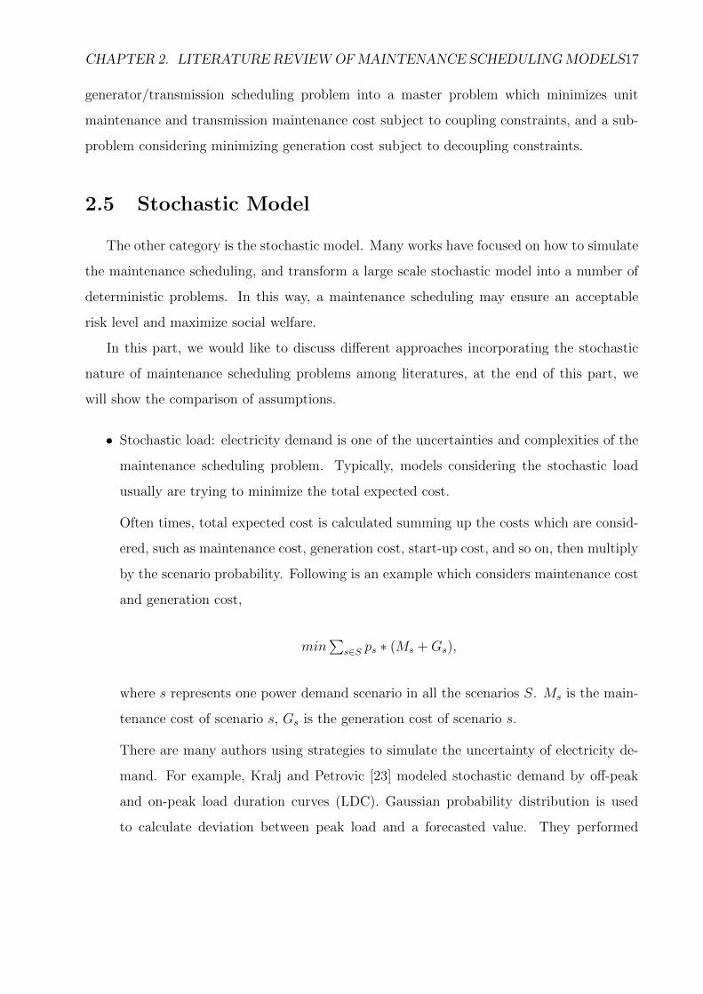
• Stochastic load: electricity demand is one of the uncertainties and complexities of the
maintenance scheduling problem. Typically, models considering the stochastic load
usually are trying to minimize the total expected cost.
Often times, total expected cost is calculated summing up the costs which are consid-
ered, such as maintenance cost, generation cost, start-up cost, and so on, then multiply
by the scenario probability. Following is an example which considers maintenance cost
and generation cost,
min∑
s∈S ps ∗ (Ms +Gs),
where s represents one power demand scenario in all the scenarios S. Ms is the main-
tenance cost of scenario s, Gs is the generation cost of scenario s.
There are many authors using strategies to simulate the uncertainty of electricity de-
mand. For example, Kralj and Petrovic [23] modeled stochastic demand by off-peak
and on-peak load duration curves (LDC). Gaussian probability distribution is used
to calculate deviation between peak load and a forecasted value. They performed

CHAPTER 2. LITERATURE REVIEWOFMAINTENANCE SCHEDULINGMODELS18
simulation before the optimization in order to save the computation during the search-
ing procedure. They treated the maintenance scheduling problem as a combinatorial
optimization task: minimizing fuel costs, maximizing reliability, and minimizing con-
straints violations simultaneously. Branch and bound is used to solve the problem.
Canto [31] formulated the maintenance scheduling problem into three demand scenar-
ios: high, medium, and low electricity demand. The possibility of each scenario is fixed
by each specific power plant, for example, in the case study, the possibility of electric
demand of a 75 power plant grid is 0.1 ( low demand ), 0.6 ( medium demand ), 0.3 (
high demand ). Each scenario is divided into 13 months, then divided into 6 subperiods
namely peak, middle, and low demand of business days and weekend days. By claiming
that maintenance cost is insignificant regarding start-up and production cost, the au-
thor does not consider maintenance cost in the objective function. The model is clearly
represented by maintenance constraints, economic unit commitment constraints, main-
tenance and connection constraints, and generating volume constraints. The problem
is solved by Bender’s decomposition.
• Uncertain forced outages of transmission lines and generating units: in Marwali and
Shahidehpour [13], whether forced outages will happen is decided at the end of a week
in the short term scheduling. Long term scheduling is determined by those forecasted
parameters. The authors used a two-state continuous-time Markov model to calculate
the forced outage rates of each utility. Then the updated value of forced outage rates are
applied to the network constraints in the long term scheduling, Monte-Carlo sampling is
used to generate 1000 random future scenarios, each of them represents the availability
of generating units and transmission lines. Then these 1000 samples are evaluated by
dynamic scheduling, using the system reserve energy as the indicator.
• Stochastic load and forced outages of generators and transmission lines: except for the
stochastic nature of demand, the uncertainty in generation capacity and transmission
line availability has also been considered. For example, Silva et al. [24] considered the
uncertainties of generators, transmission lines, and peak load of certain areas defined
by stochastic vectors. The operation subproblem aimed at minimizing the expected

CHAPTER 2. LITERATURE REVIEWOFMAINTENANCE SCHEDULINGMODELS19
energy not served (EPNS). The operation subproblem is checked with a pre-established
upper bound on EPNS in the original problem. First, the master problem (decision)
establishes a trial maintenance schedule subjected to resource, sequence and other
constraints. This result is one of the stochastic vectors. Then this vector is checked in
the operation sub problem. If the trail schedule does not violate operation subproblem
reliability constraint, the proposed trial schedule is optimal. Otherwise, Benders cut
is generated and added to the master problem. This procedure is performed until
convergence.
• Uncertainties in prices of energy, ancillary services, and fuel: from the GENCO’s point
of view, the goal is to maximize its payoffs and minimize its financial risk. The payoff
of a GENCO is highly dependent on the prices of energy, ancillary services, and fuel.
If a GENCO could adjust its maintenance outage to periods when the prices of energy
and ancillary services are relatively low and the price of fuel is high, it could save a
lot of money. In Wu et al. [14], the author realized this coordination by Monte Carlo
simulation. First, a stochastic maintenance scheduling model which maximizes the
GENCOS’s payoff subject to maintenance outage windows and resource constraints is
proposed, then it introduces hourly priced-based unit commitment constraints includ-
ing energy, ancillary services, fuel constraints, and many other constraints. Following
is the objective function which incorporates uncertain prices in scenarios,
max∑
s∈S∑
t∈T ps ∗ {Gt,(s) + St,(s) +NSt,(s) +Bt,(s) − (Mt,(s) + Ft,(s) + SDt,(s))},
where Gt,(s), St,(s), NSt,(s), Bt,(s) represent generation income, spinning reserve income,
non-spinning reserve income, and bilateral income of scenario s in period t, Mt,(s), Ft,(s),
SDt,(s) represent maintenance cost, fuel cost, and shut down cost of scenario s in period
t.
Monte carlo method is used to generate all initial scenarios, each of them has an
associated probability. After checking the bundle constraints, each scenario subproblem
is solved in order to maximize payoffs in the entire period. Once a trial schedule is
obtained, fuel, emission, and maintenance coupling constraints are checked. If all the

CHAPTER 2. LITERATURE REVIEWOFMAINTENANCE SCHEDULINGMODELS20
constraints are not violated, go to the next scenario, otherwise recalculate the problem
by updating Lagrangian multipliers. After the solution for all the scenarios are found,
an optimal schedule is obtained if the solution does not violate the bundle constraints
among scenarios.
• Stochastic forced outages, fuel prices,and load forecast errors
In Wu et al. [15], Lagrangian relaxation is used to decompose the original problem,
moreover, the Monte Carlo method is used to simulate the random outages of gener-
ators and transmission lines, fuel price fluctuations and load forecast errors. Scenario
bundle constraints are decomposed in long term security-constrained UC subproblem,
thus the final solution is a combination of weighted scenarios. The objective function
is
min∑
s∈S∑
t∈T{Mt,(s) + ps ∗ (Ft,(s) + SDt,(s) + SUt,(s)) + Pt,(s)},
where SUt,(s), Pt,(s) represent start up cost and penalty cost of scenario s in period t.
As we showed before, the uncertainty of forced outages of generating units and trans-
mission lines, the load forecast errors, the fluctuation in energy, ancillary services, and
fuel prices are all key items considered in stochastic maintenance scheduling models.
In Table 2.5, some authors choose one of them to deal with, some choose the combina-
tion of them. The key point in proposing a stochastic maintenance scheduling model
is how to simulate different scenarios, each of them has a corresponding probability.
Branch-and-bound and Monte-Carlo simulation are used to realize that goal.

CHAPTER 2. LITERATURE REVIEWOFMAINTENANCE SCHEDULINGMODELS21
Assumptions ReferencesPower demand in each time period is mod-eled by load duration curves
[25], [23], [46], [47], [24], [30],[22], [48], [15]
The fluctuation in prices of fuel, energy,and ancillary services could influence aGENCO’s payoff
[21], [14], [15]
Forced outage rate is considered [46], [47], [30], [24], [30], [21],[15]
Table 2.5: Summary of assumptions in stochastic model

22
Chapter 3
Power Plant Maintenance Considering
Fuel Contracts
In this chapter the assumptions of maintenance scheduling with gas portfolio have been
made. A novel optimization model of maintenance scheduling is proposed including model
reformulation and decomposition. Finally the computational results among the original
model, reformulated model and decomposed model have been compared.
3.1 Problem Statement
This section introduces the logic and assumptions in the model. A Take-or-Pay gas
portfolio is proposed. The rule of gas transfer between reservoirs and power plant has been
defined.
3.1.1 Maintenance Scheduling with Gas Portfolio
In previous chapters we have introduced the maintenance within power plant itself. How-
ever the power plant is not isolated from the outside pool. All the market participants, such
as GENCOS, TRANSCOS, and DISCOS, are closely related to power plants [49]. Henceforth
many researchers have not only considered maintenance modeling within power plant, they
have also took other participants into consideration. In this research, we assume that we

CHAPTER 3. POWER PLANTMAINTENANCE CONSIDERING FUEL CONTRACTS23
are dealing with a power plant that runs on natural gas, a non-renewable resource. This as-
sumption has motivated us to consider maintenance with gas portfolio because every natural
gas power station needs to deal with gas purchasing.
Gas portfolio optimization is performed to optimally use the flexibility in gas purchasing
[50]. It helps reduce the risks and costs in a gas portfolio when decision making is needed
by managers, investors and traders. The uncertain demand is the first priority to be served.
For example, in a power plant using natural gas generating electricity, the demand of gas
is uncertain due to the uncertain demand of electricity from customers, maintenance of
generating units, and so on. Then several aspects should be considered to meet the demand,
such as gas purchasing price, gas spot market trading, and gas storage reservoir capacity.
Gas portfolio optimization could contribute to the reduction of gas costs, and avoid buying
gas from gas spot market at high price or not being able to meet demand.
The main goal of combining gas contract optimization and power plant maintenance
scheduling is to decrease the cost for both purchasing gas and performing maintenance,
and increase the revenue from power generation. Since the gas price and electricity price
are fluctuating all the time, so these two factors are the main sources driving our model.
Our goal is to purchase gas when gas price is relatively low, and postpone maintenance
when electricity price is relatively high but not overuse the power generating units without
maintenance.
Take-or-Pay Gas Contract
We consider a Take-or-Pay(ToP) gas contract in this project. A Take-or-Pay gas con-
tract is a rule established between companies and gas suppliers [51]. The company must
take an agreed amount of gas from the supplier [52]. We model the Take-or-pay gas con-
tract with the maximum monthly gas withdraw volume of M , together with the minimum
monthly withdraw percentage X%. We also have an annual minimum withdraw percentage
of Y%(Y ≥ X), and maximum storage time of gas of N periods. The following assumptions
are made in this project:
• Two reservoirs are considered, A and B. Reservoir B is the receiver of yearly gas volume,
and it can transfer gas to reservoir A in every month. Reservoir A is the receiver of

CHAPTER 3. POWER PLANTMAINTENANCE CONSIDERING FUEL CONTRACTS24
monthly gas volume from both reservoir B and the distributors, and it can transfer gas
to the power plant.
• Gas in reservoir A must be less than or equal to the maximum monthly gas withdraw
volume of M , and greater than or equal to the minimum monthly gas withdraw volume
of X%M .
• At the beginning of each year, Y% ∗ 12M amount of gas is pushed into reservoir B.
• Reservoirs A and B must be restored to full capacity at the end of each year.
Figure 3.1 points out the gas transfer direction in our assumptions. It shows the ToP
gas contract. If gas from the ToP contract cannot meet the demand of power plant, it will
directly purchase gas from the spot market, and it can also sell the redundant gas to spot
market.
Reservoir B Reservoir A
Power Plant
Spot Market
Distributor
Figure 3.1: Gas transfer direction
Maintenance Factors
As we surveyed previously, there are a lot of factors one can consider in maintenance
scheduling, such as maintenance duration, resource, priority, and so on. In this project, we
consider three factors, namely maintenance duration, frequency, and maintenance cost. Table
3.1 shows an example of maintenance-related frequency, duration, and cost in a moderate-size
power plant.

CHAPTER 3. POWER PLANTMAINTENANCE CONSIDERING FUEL CONTRACTS25
Equipment Time between maintenance Average Duration Cost($)
1 2300 hours 7 days 11002 2600 hours 14 days 13003 2800 hours 21 days 1900
Table 3.1: Maintenance factors
3.1.2 The Assumptions
To facilitate the model formulation, the mathematical model has the following assump-
tions:
1. Electricity generated can always be sold to the market.
2. The maximum storage time of gas in reservoirs A&B is one year.
3. All maintenance performed has fixed amount of time and cost, and no contingency
exist.
4. The gas usage per day of the power plant is a constant.
5. Gas availability is stable as long as it satisfies our gas contract logic.
3.2 Stochastic Model
Based on the assumptions and logic stated in previous section, this section introduces
the original stochastic optimization model including objectives and constraints.
3.2.1 Introduction to Stochastic Programming
Compared with deterministic problems, stochastic problems take uncertainties into con-
sideration [53]. The stochastic programming model is more suitable to describe the problems
since unknown parameter exists in the real world. In stochastic programming models, un-
certainty is expressed in probabilities. The series of events and actions which are possible to
happen are called scenarios. Most of stochastic problems have probability distributions for

CHAPTER 3. POWER PLANTMAINTENANCE CONSIDERING FUEL CONTRACTS26
scenarios. The optimization goal is to minimize or maximize the expectations of objective
function [54].
A stage is a point of progress. Decisions must be made in each stage. In a two stage
stochastic model, a set of decisions need to be made without full information on some random
events [55]. These decisions are called first-stage decisions. The second-stage or corrective
actions are taken when full information is received on the realization of some random factor
[56].
The multistage stochastic programming problems is an extension of the two stage prob-
lems described above. A sequence of observations ξ1, ξ2, ..., ξt will be used as decision making
criterion. The current stage decisions are made based on previous observations. Figure 3.2
shows the multistage decision process[57].
Figure 3.2: Multistage decision process
Let node 1 to be the root node. Since a decision needs to be made without full information
when t = 1, there is only one node in the first stage. After the first stage, if we assume
that there are two uncertainties in each stage, then every node will generate two nodes in
the following stage. Let a(n) be the ancestor of node n. Figure 3.3 shows the scenario tree
with three stages. If node n is a leaf node, then the path from the root node to n is called
a scenario (k) [58]. Each scenario has a corresponding probability (Pk).
In our model, multistage stochastic model is applied. Each month is considered as a stage.
Gas and electricity price in each month will be the uncertainties which could influence the
maintenance and power generation decisions.

CHAPTER 3. POWER PLANTMAINTENANCE CONSIDERING FUEL CONTRACTS27
Figure 3.3: Scenario tree
Indices Descriptionsξ Senariosi Maintenance equipmentst Time period(days, months or years)T Time horizon to be considered(years)T0 Beginning of each yearTE End of each yearn Scenario bundles nodej columns
Table 3.2: Indices
3.2.2 General Nomenclature
The indices, parameters and variables used in the stochastic model are showed in Table
3.2, 3.3, 3.4.
3.2.3 Objective Function
The objective of this study is to minimize negative of the total profit of electricity gen-
eration over the planning horizon. probξ means the probability of the occurrence of each
scenario ξ; cξt (mξt + f ξt ) is the gas purchasing cost from the contract, and qξt s
ξt
−is the gas
purchasing cost from spot market; hξt (gξt +sξt
−) is the revenue coming from selling electricity,
and pξtsξt
+is the income for selling redundant gas to spot market; uiz
ξi,t is the maintenance
CHAPTER 3. POWER PLANTMAINTENANCE CONSIDERING FUEL CONTRACTS28
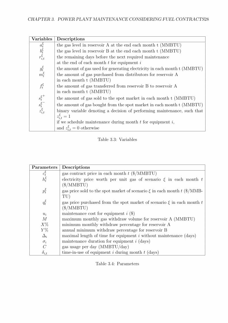
Variables Descriptions
aξt the gas level in reservoir A at the end each month t (MMBTU)
bξt the gas level in reservoir B at the end each month t (MMBTU)
rξi,t the remaining days before the next required maintenanceat the end of each month t for equipment i
gξt the amount of gas used for generating electricity in each month t (MMBTU)
mξt the amount of gas purchased from distributors for reservoir A
in each month t (MMBTU)
f ξt the amount of gas transferred from reservoir B to reservoir Ain each month t (MMBTU)
sξt+
the amount of gas sold to the spot market in each month t (MMBTU)
sξt−
the amount of gas bought from the spot market in each month t (MMBTU)
zξi,t binary variable denoting a decision of performing maintenance, such thatzξi,t = 1if we schedule maintenance during month t for equipment i,
and zξi,t = 0 otherwise
Table 3.3: Variables
Parameters Descriptions
cξt gas contract price in each month t ($/MMBTU)
hξt electricity price worth per unit gas of scenario ξ in each month t($/MMBTU)
pξt gas price sold to the spot market of scenario ξ in each month t ($/MMB-TU)
qξt gas price purchased from the spot market of scenario ξ in each month t($/MMBTU)
ui maintenance cost for equipment i ($)M maximum monthly gas withdraw volume for reservoir A (MMBTU)X% minimum monthly withdraw percentage for reservoir AY% annual minimum withdraw percentage for reservoir B∆i maximal length of time for equipment i without maintenance (days)σi maintenance duration for equipment i (days)C gas usage per day (MMBTU/day)δi,t time-in-use of equipment i during month t (days)
Table 3.4: Parameters

CHAPTER 3. POWER PLANTMAINTENANCE CONSIDERING FUEL CONTRACTS29
cost. The total profit is the summation of the above items with income having a negative sign
and outcome having a positive sign. The objective function can be represented as follows,
min∑
ξ∈Ξ probξ[∑
t∈T (cξt (mξt + f ξt )− hξt (g
ξt + sξt
−)− pξts
ξt
++ qξt s
ξt
−) +
∑i∈I
∑t∈T uiz
ξi,t]
3.2.4 Constraints
The motivation in this project is to consider both maintenance part and gas portfolio
part, and then connect those two with their relationships. The motivation is represented by
the following constraints.
Gas Balance In Reservoirs
In this model, we consider the gas balance in reservoir A and B between one month and
the previous month. For reservoir A, the input is the amount of gas purchased from distrib-
utors (mξt ) and transferred from reservoir B (f ξt ), and the output will be the amount of gas
sold to the spot market (sξt+
) and used for electricity generation (gξt ). For each scenario ξ
and each time period t, gas balance constraint can be represented as follows:
aξt = aξt−1 +mξt + f ξt − s
ξt
+ − gξt
For reservoir B, there will be only one output, that is the amount of gas transferred to
reservoir A (f ξt ):
bξt = bξt−1 − fξt
Gas Transfer Logic
According to the assumption, for reservoir A, the maximum monthly gas withdraw vol-
ume is M , and the minimum gas withdraw percentage is X%. Again, for each scenario ξ
and each time period t, gas transfer logic can be represented as follows:
X%M ≤ mξt + f ξt ≤M

CHAPTER 3. POWER PLANTMAINTENANCE CONSIDERING FUEL CONTRACTS30
For reservoir B, the annual minimum withdraw percentage is Y%:
bξt = Y%(12M)− f ξt
Also, reservoir A and B must be restored to full capacity at the end of the maximum storage
time N , and if N is one year, then the following constraints are established:
bξt = 0, aξt = 0
when t = 12.
Maintenance Logic
At the end of each month t, the remaining days before the next required maintenance
(rξi,t) should be related with the maintenance decision (zξi,t) and electricity generation (δi,t) in
each month t. Maintenance logic for each scenario ξ, each equipment i and each time period
t can be represented as follows:
rξi,t ≤ rξi,t−1 − δi,t + (∆i + σi)zξi,t
The upper bound of rξi,t should be the maximum days without maintenance minus the usage
of equipment i in each month t:
rξi,t ≤ ∆i + σi − δi,t
Power Generation Logic
The amount of gas used for electricity generation in each month t should be related with
the maintenance decision. The lower number of maintenance happened in one month, the
higher amount of gas would be consumed to generate electricity:
gξt + sξt− ≤ C(δi,t − σizξi,t)

CHAPTER 3. POWER PLANTMAINTENANCE CONSIDERING FUEL CONTRACTS31
Nonanticipativity Constraint
We use Sn,t to denote scenario bundles node n if scenario ξ and η have the same history
until time t at node n, so variables related with node n should have the same decisions in
time t:
xξt = xηt , ∀(ξ, η) ∈ Sn,t
where xξt = [aξt , bξt , g
ξt , s
ξt
+, sξt
−, mξ
t , fξt , z
ξt , r
ξt ].

CHAPTER 3. POWER PLANTMAINTENANCE CONSIDERING FUEL CONTRACTS32
3.2.5 Optimization Model
The general stochastic programming model is summarized as follows:
min∑ξ∈Ξ
probξ[∑t∈T
(cξt (mξt + f ξt )− hξt (g
ξt + sξt
−)− pξts
ξt
++ qξt s
ξt
−) +
∑i∈I
∑t∈T
uizξi,t] (3.1)
s.t. aξt = aξt−1 +mξt + f ξt − s
ξt
+ − gξt , ∀t ∈ T, ξ ∈ Ξ, (3.2)
bξt = bξt−1 − fξt , ∀t ∈ T\T0, ξ ∈ Ξ, (3.3)
X%M ≤ mξt + f ξt ≤M, ∀t ∈ T, ξ ∈ Ξ, (3.4)
bξt = Y%(12M)− f ξt , ∀t ∈ T0, ξ ∈ Ξ, (3.5)
bξt = 0, aξt = 0, ∀t ∈ TE, ξ ∈ Ξ, (3.6)
rξi,t ≤ rξi,t−1 − δi,t + (∆i + σi)zξi,t, ∀t ∈ T\1, ξ ∈ Ξ, i ∈ I, (3.7)
gξt + sξt− ≤ C(δi,t − σizξi,t), ∀t ∈ T, ξ ∈ Ξ, i ∈ I, (3.8)
rξi,t ≤ ∆i + σi − δi,t, ∀t ∈ T, ξ ∈ Ξ, i ∈ I, (3.9)
xξt = xηt , ∀(ξ, η) ∈ Sn,t, t ∈ T, n ∈ N, ξ ∈ Ξ, (3.10)
zξi,t ∈ {0, 1}, ∀t ∈ T, i ∈ I, ξ ∈ Ξ, (3.11)
aξt , bξt , g
ξt , s
ξt
+, sξt
−, mξ
t , fξt , r
ξi,t ≥ 0 ∀t ∈ T, i ∈ I, ξ ∈ Ξ, (3.12)
where xξt = [aξt , bξt , g
ξt , s
ξt
+, sξt
−, mξ
t , fξt , z
ξt , r
ξt ], zξt = [ zξ1,t, . . . , z
ξi,t], rξt = [ rξ1,t, . . . , r
ξi,t].
ξ denotes scenarios. Constraint (3.2) and (3.3) show the balance of gas level in reservoir A
and B in each period. Constraint (3.4) points out the upper and lower bound of monthly
withdraw volume. Constraint (3.10) is the nonanticipativity constraint.
3.3 Model Reformulation
We can interpret maintenance in the way that maintenance in one period must be per-
formed so that the decreasing of capacity of the equipment can be restored. In this way,
maintenance is considered as replenishment to the usage of the equipment. We can also
consider that the maintenance in one period will affect the following periods such as the
maintenance decisions in those periods. In other words, maintenance is considered as an
action which will impact the following periods. If maintenance is interpreted in the second

CHAPTER 3. POWER PLANTMAINTENANCE CONSIDERING FUEL CONTRACTS33
way, we need to answer how it affect the following periods and what is the contribution of
one maintenance in terms of meeting the capacity requirements in the following periods.
The main contribution of reformulation is obtaining a tighter approximation of the convex
hull of feasible solutions so that the computational speed will be faster [59]. We use ζ iτt
to denote whether maintenance of i in period τ contributes toward meeting the capacity
requirement of i in period t, φi denotes equipment i should be maintained every φ months,
and τ denotes time periods (days, months, or years).
Figure 3.4 shows that if one equipment must been maintained every three months, then we
can split maintenance decision variable in time period 3 (z3) into three variables: ζ13, ζ23, ζ33.
Instead of analyzing z3, we are now interested in what will affect z3 using ζ13, ζ23, ζ33.
Figure 3.4: Reformulation technique
According to [59], if the summation of ζ iτt is greater or equal to 1 which means at least
there will be one ζ iτt contribute toward meeting the capacity requirement in the following
τ periods, the equipment will be in good condition since all the necessary maintenance has
been performed. So constraint (3.7)&(3.9) can be reformulated as
ζt−τ,t ≤ zt−τ , ∀τ ∈ [0, φi − 1], (3.13)φi−1∑τ=0
ζt−τ,t ≥ 1. (3.14)
According to the previous principles, the original stochastic programming model can be
developed to a reformulated model as follows:

CHAPTER 3. POWER PLANTMAINTENANCE CONSIDERING FUEL CONTRACTS34
min∑ξ∈Ξ
probξ[∑t∈T
(cξt (mξt + f ξt )− hξt (g
ξt + sξt
−)− pξts
ξt
++ qξt s
ξt
−+∑i∈I
∑t∈T
uizξi,t](3.15)
s.t. aξt = aξt−1 +mξt + f ξt − s
ξt
+ − gξt , ∀t ∈ T, ξ ∈ Ξ, (3.16)
bξt = bξt−1 − fξt , ∀t ∈ T\T0, ξ ∈ Ξ, (3.17)
X%M ≤ mξt + f ξt ≤M, ∀t ∈ T, ξ ∈ Ξ, (3.18)
bξt = Y%(12M)− f ξt , ∀t ∈ T0, ξ ∈ Ξ, (3.19)
bξt = 0, aξt = 0, ∀t ∈ TE, ξ ∈ Ξ, (3.20)
ζξi,t−τ,t ≤ zξi,t−τ , ∀τ ∈ [0, φi − 1], t ∈ T, ξ ∈ Ξ, i ∈ I, (3.21)
φi−1∑τ=0
ζξi,t−τ,t ≥ 1, ∀t ∈ T, ξ ∈ Ξ, i ∈ I, (3.22)
gξt + sξt− ≤ C(δi,t − σizξi,t), ∀t ∈ T, ξ ∈ Ξ, i ∈ I, (3.23)
xξt = xηt , ∀(ξ, η) ∈ Sn,t, t ∈ T, n ∈ N, ξ ∈ Ξ, (3.24)
ζξi,t−τ,t ∈ {0, 1}, ∀τ ∈ [0, φi − 1], t ∈ T, ξ ∈ Ξ, i ∈ I, (3.25)
0 ≤ zξi,t ≤ 1, ∀t ∈ T, ξ ∈ Ξ, i ∈ I, (3.26)
aξt , bξt , g
ξt , s
ξt
+, sξt
−, mξ
t , fξt ≥ 0 ∀t ∈ T, ξ ∈ Ξ (3.27)
3.4 Decomposition
If we enlarge the problem, there will be a bottleneck that the computer cannot solve
the model due to insufficient memory since there are too many feasible solutions for the
computer to find all of them. In this case, decomposition could help solve large-scaled prob-
lems. The main idea of decomposition is that starting solving the model when some of the
feasible solutions have been obtained serving as basis, then use this basis to search for more
feasible solutions. When no more feasible solution can help improve the objective value, the
combination of current feasible solutions is optimal. We use Dantzig-Wolfe Decomposition
technique to further decompose the reformulated model [59].
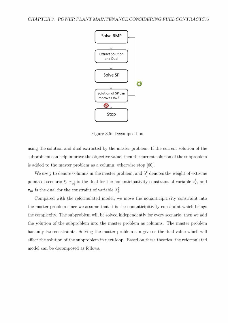
Figure 3.5 shows the Dantzig-Wolfe Decomposition procedure. The master problem is
solved initially, and the solution and dual are extracted. Then the subproblem is solved
CHAPTER 3. POWER PLANTMAINTENANCE CONSIDERING FUEL CONTRACTS35
Solve RMP
Extract Solution and Dual
Solve SP
Solution of SP can improve Obv?
Stop
Figure 3.5: Decomposition
using the solution and dual extracted by the master problem. If the current solution of the
subproblem can help improve the objective value, then the current solution of the subproblem
is added to the master problem as a column, otherwise stop [60].
We use j to denote columns in the master problem, and λξj denotes the weight of extreme
points of scenario ξ. πxξtis the dual for the nonanticipativity constraint of variable xξt , and
π0ξ is the dual for the constraint of variable λξj .
Compared with the reformulated model, we move the nonanticipitivity constraint into
the master problem since we assume that it is the nonanticipitivity constraint which brings
the complexity. The subproblem will be solved independently for every scenario, then we add
the solution of the subproblem into the master problem as columns. The master problem
has only two constraints. Solving the master problem can give us the dual value which will
affect the solution of the subproblem in next loop. Based on these theories, the reformulated
model can be decomposed as follows:

CHAPTER 3. POWER PLANTMAINTENANCE CONSIDERING FUEL CONTRACTS36
SB-MP:
min∑ξ∈Ξ
probξ∑j∈Jξ
Rξjλ
ξj (3.28)
s.t.Wxn −∑j∈Jξ
(xξt )jλξj = 0, ∀(ξ, t) ∈ Sn, n ∈ N, [πxξt
] (3.29)
∑j∈Jξ
λξj = 1, ∀ξ ∈ Ξ, [πξ0] (3.30)
0 ≤ λξj ≤ 1, ∀j ∈ Jξ, ξ ∈ Ξ, (3.31)
where (xξt )j = [(aξt )
j, (bξt )j, (mξ
t )j, (f ξt )j, (gξt )
j, (sξ+t )j, (sξ−t )j, (zξt )j], (zξt )
j = [(zξ1,t)j, . . . , (zξi,t)
j],
Rξj =
∑t∈T [cξt ((m
ξt )j + (f ξt )j)− hξt ((g
ξt )j + (sξ−t )j)− pξt (s
ξ+t )j + qξt (s
ξ−t )j] +
∑t∈T
∑i∈I ui(z
ξi,t)
j.
SB-SP(ξ):
min∑t∈T
[(cξt + πmξt)mξ
t + (cξt + πfξt)f ξt − (hξt − πgξt )g
ξt − (hξt − πsξ−t )sξ−t (3.32)
−(pξt − πsξ+t )sξ+t + (qξt + πsξ−t)sξ−t + πaξt
aξt + πbξtbξt ] (3.33)
+∑t∈T
∑i∈I
(ui + πzξi,t)zξi,t − π
ξ0 (3.34)
s.t. aξt = aξt−1 +mξt + f ξt − s
ξt
+ − gξt , ∀t ∈ T, (3.35)
bξt = bξt−1 − fξt , ∀t ∈ T\T0, (3.36)
X%M ≤ mξt + f ξt ≤M, ∀t ∈ T, (3.37)
bξt = Y%(12M)− f ξt , ∀t ∈ T0, (3.38)
bξt = 0, aξt = 0, ∀t ∈ TE, (3.39)
ζξi,t−τ,t ≤ zξi,t−τ , ∀τ ∈ [0, φi − 1], t ∈ T, i ∈ I, (3.40)
φi−1∑τ=0
ζξi,t−τ,t ≥ 1, ∀t ∈ T, i ∈ I, (3.41)
gξt + sξt− ≤ C(δi,t − σizξi,t), ∀t ∈ T, i ∈ I, (3.42)
ζξi,t−τ,t ∈ {0, 1}, ∀τ ∈ [0, φi − 1], t ∈ T, i ∈ I, (3.43)
0 ≤ zξi,t ≤ 1, ∀t ∈ T, i ∈ I, (3.44)
aξt , bξt , g
ξt , s
ξt
+, sξt
−, mξ
t , fξt ≥ 0, ∀t ∈ T, i ∈ I. (3.45)

CHAPTER 3. POWER PLANTMAINTENANCE CONSIDERING FUEL CONTRACTS37
3.5 Computational Results
In this chapter, the solution of the original stochastic model is firstly analyzed. Then we
compare the solution of the reformulated model with the original one to see whether they
have the same result. Thirdly, the contribution of decomposition is discussed.
3.5.1 Analyze the Solution of the Original Model
We initially obtained all the rough data on Energy Information Administration. In order
to show the effectiveness of the original model, we would like to see if we manipulate the
data such as making the data higher in the first 6 months and lower in the following 6
months, the model will certainly give us logical solutions according to that manipulation.
For this purpose, we manipulated cξt , qξt and hξt higher/lower in the first half of the year and
lower/higher in the rest of the year, and we kept pξt to be a very low value since we do not
want to purchase any redundant gas and sold them to the spot market. The parameters
used are as follows:
TimePeriod
1 2 3 4 5 6 7 8 9 10 11 12
cξt 2.12 2.13 2.21 2.31 2.05 2.07 2.93 2.92 2.73 2.99 2.89 2.88
qξt 2.66 2.76 2.73 2.63 2.83 2.70 2.32 2.31 2.28 2.15 2.22 2.18
hξt 11.83 11.79 11.71 11.89 11.76 11.86 9.95 9.96 9.88 9.89 9.91 9.92
pξt 1 1 1 1 1 1 1 1 1 1 1 1
Table 3.5: Input parameters of prices($/MMBTU)
Scenario# Unit# ∆i(day) σi(day) ui($)1 1 87 7 1000
Table 3.6: Other parameters
The model was solved by IBM Cplex Optimization Studio. The objective value and
solution reported by Cplex are as follows:
The maintenance decision reflects that the equipment must be maintained at least every
3 months which makes sense because we used 87 days as the longest time of one unit without

CHAPTER 3. POWER PLANTMAINTENANCE CONSIDERING FUEL CONTRACTS38
Objective Value -481717
Table 3.7: Objective value of the original model using parameters in Table 3.5 & 3.6
TimePeriod
1 2 3 4 5 6 7 8 9 10 11 12
mξt 0 5000 5000 5000 0 0 0 1000 0 1000 1000 0
f ξt 5000 0 0 0 5000 5000 1000 0 1000 0 0
sξ−t 200 0 0 0 0 0 2120 2910 4100 5100 1910 4100
gξt 4900 5100 3910 5100 3910 5100 2980 1000 1000 0 2000 1000
sξ+t 0 0 0 0 0 0 0 0 0 0 0 0
zξi,t 0 0 1 -0 1 -0 0 1 0 0 1 -0
rξi,t 57 27 30 0 64 34 4 60 30 0 30 0
aξt 100 0 1090 990 2080 1980 0 0 0 1000 0 0
bξt 13000 13000 13000 13000 8000 3000 2000 2000 1000 1000 1000 0
Table 3.8: Solution of the original model using parameters in Table 3.5 & 3.6
maintenance. Also, we can interpret from the solution that the model is able to select the
optimal gas sources, that is, when gas price in ToP contract is low, then ToP is selected as
the gas source, when gas price from the distributor is low, then the distributor will provide
gas. Finally, the electricity generation is significantly affected by the electricity price. For
example, the amount of electricity generated in the first six months is much higher than the
second half of the year due to the relatively high electricity price. Also, no gas has been sold
to the spot market because the spot market selling price is very low. So model can responde
to different input data and the solution makes sense.
3.5.2 Compare the Solution and Computational Time of the O-
riginal and Reformulated Model
Compare the Solution
It is clear from Table 3.7 and 3.9 that the objective value of the reformulated model is
exactly the same as the original one, and the solutions of the reformulated model are slightly
different with the original ones since alternative solutions may exit. This indicates that
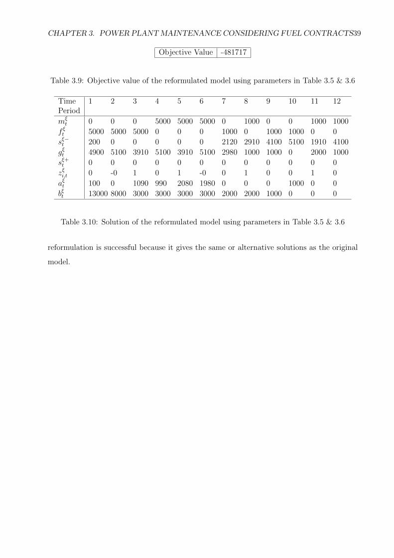
CHAPTER 3. POWER PLANTMAINTENANCE CONSIDERING FUEL CONTRACTS39
Objective Value -481717
Table 3.9: Objective value of the reformulated model using parameters in Table 3.5 & 3.6
TimePeriod
1 2 3 4 5 6 7 8 9 10 11 12
mξt 0 0 0 5000 5000 5000 0 1000 0 0 1000 1000
f ξt 5000 5000 5000 0 0 0 1000 0 1000 1000 0 0
sξ−t 200 0 0 0 0 0 2120 2910 4100 5100 1910 4100
gξt 4900 5100 3910 5100 3910 5100 2980 1000 1000 0 2000 1000
sξ+t 0 0 0 0 0 0 0 0 0 0 0 0
zξi,t 0 -0 1 0 1 -0 0 1 0 0 1 0
aξt 100 0 1090 990 2080 1980 0 0 0 1000 0 0
bξt 13000 8000 3000 3000 3000 3000 2000 2000 1000 0 0 0
Table 3.10: Solution of the reformulated model using parameters in Table 3.5 & 3.6
reformulation is successful because it gives the same or alternative solutions as the original
model.

CHAPTER 3. POWER PLANTMAINTENANCE CONSIDERING FUEL CONTRACTS40
0
5
10
15
20
25
30
35
40
45
10 33 50 75 100 125 150
com
pu
tati
on
al t
ime/
sec
i
t=6
Ori Ref
Figure 3.6: Compare computational time when t=6
Compare the Computational Time
Except for the effectiveness of the reformulation, we are more interested with the effi-
ciency. For this purpose, we continuously increased the number of period t and the number
of equipment i. We assumed that there will be 2 uncertainties in each time period, and the
random data are generated in Excel based on the rough data obtained on Energy Informa-
tion Administration. For example, if we consider 6 periods, the number of scenarios would
be 25 = 32. Figure 3.6, 3.7, and 3.8 compare the computational time between the original
and reformulated models when we consider different time horizon and different number of
equipment.
The reformulated model is very efficient when the time horizon considered is relatively
short and the number of equipment is low. For example, when t=9, and i=33, the computa-
tional time of reformulation is only 17 seconds, while the original model needs 150 seconds.
However, when we consider long time horizon and large number of equipment, the efficiency
will drop. This is one part of the future research, that is, making the reformulated model

CHAPTER 3. POWER PLANTMAINTENANCE CONSIDERING FUEL CONTRACTS41
0
50
100
150
200
250
300
350
400
10 33 50 75 100 125 150
com
pu
tati
on
al t
ime/
sec
i
t=9
Ori Ref
Figure 3.7: Compare computational time when t=9
0
1000
2000
3000
4000
5000
6000
7000
8000
9000
10 33 50 75 100 125 150
com
pu
tati
on
al t
ime/
sec
i
t=12
Ori Ref
Figure 3.8: Compare computational time when t=12

CHAPTER 3. POWER PLANTMAINTENANCE CONSIDERING FUEL CONTRACTS42
efficient when dealing with large-scale problems.
3.5.3 Solution of the Decomposed Model
We have selected number of time periods being 6 and number of scenarios being 32. Since
Wzn is the maintenance decision in the decomposed model, the evolution of Wzn during loops
will indicate how decomposition works. The solution of Wzn has been extracted and showed
in Table 3.11 and 3.12:
In the first loop, all the Wzn are binary and the objective value is -250237. The objective
value continued decreasing as the number of loops increases. In the 22nd loop, the objective
value is -257575 and Wzn became decimal. After the 29th loop, the objective value remained
-257946 and nearly all the Wzn are binary solutions with only four Wzn being decimals.
This is the best solution our decomposed model can obtain so far. What is expected from
the decomposed model is that the upper bond and lower bond should converge quickly and
all the Wzn are binary when the objective value remains the same and cannot be further
improved. This is also part of the future research.
3.6 Conclusions and Future Research
As we surveyed in Chapter 2, there are many kinds of decisions, constraints, and ob-
jectives used in previous literature of power plant maintenance scheduling. We established
the assumption that we are dealing with the power plant using natural gas as resources, so
gas portfolio should be considered in the model. Based on that assumption, least-cost based
criterion is selected as objective since our primary goal is to minimize maintenance and pro-
duction cost, as well as maximizing revenues. Also, a couple of constraints are established
specifying maintenance logic, power generation logic, gas purchasing, and the relationship
among those. Some variables are defined to represent maintenance decision, power genera-
tion, and gas reservoir status. The model is considered as a stochastic one since the possible
combinations of data have been used as input.
The computational result of the original stochastic model indicates that if the input data
has some general pattern, the model will return logical solutions according to the data. For

CHAPTER 3. POWER PLANTMAINTENANCE CONSIDERING FUEL CONTRACTS43
example, the model would tell the decision maker where gas should be purchased and how
much should be purchased according to gas price of different resources such as spot market
and gas contract, the model also tells that how much electricity should be generated in
each period. The most important aspect is that the model ensures that all the maintenance
requirements are satisfied. The optimal objective value indicates how much profit will be
generated under current data. However, computational speed of the original model is not
very satisfying which motivated us to find better model formulations.
Maintenance problems can be considered as capacity planning problems. One reformula-
tion technique has been successfully applied on capacity planning problems by splitting the
capacity expansion variables into multiple ones. The benefit is obtaining a tighter convex
hull which could help reduce computational time. We applied this reformulation technique
on our maintenance decision variables, trying to analyze the effect of maintenance by ask-
ing what does one maintenance mean and how will it affect the following maintenances, in
other words, what is the contribution of one maintenance in terms of meeting the capacity
requirements in the following periods. The computational results of the reformulated model
is satisfying because the reformulation not only gives us the optimal solution but also takes
much less computational time. But the reformulation also has some bottleneck. The ad-
vantage of reformulation becomes less obvious as we expand the problem. This called us to
propose decomposition.
When problem size is so large that no matter how powerful the computer is, the problem
still cannot be solved by Cplex and it even cannot return one feasible solution because there
are too many feasible solutions for Cplex to find all of them. Decomposition has some
advantages in this situation. The main idea of decomposition is to only consider part of the
feasible solutions. When part of the feasible solutions have been found, decomposition will
add more feasible solutions through loops under the assumption that those added feasible
solutions can help improve the objective value. Otherwise, when no further feasible solution
can improve the objective value, the process will be terminated and we claim that the
combination of current feasible solutions is optimal. Now this algorithm has already been
achieved in Cplex: from the example computational results of decomposition we can see that
the objective value has been improved continuously as more and more columns are added

References 44
into the model. But we did not obtain the optimal solution since some of the maintenance
decision variables are not binary. As we discussed before, decomposition starts from some
basic feasible solutions. In order to find the optimal solution of decomposition, we may
improve the original feasible solutions added to the model serving as basis by either changing
the number of feasible solutions added at the beginning of decomposition or changing the
data used to obtain those original feasible solutions.
Since the reformulated model is efficient only when the problem size is small. We did not
obtain the optimal solution from the decomposed model, and the converging speed is very
slow. Future work will focus on the following areas:
• Accelerate the computational speed of the reformulated model, enable it to solve large-
scale problems very quickly.
• Accelerate the converging speed of the decomposed model so that the optimal solution
can be obtained in a reasonable time.
• The proposed optimization model will be evaluated by comparing computational results
with production schedules obtained in the real world.

References 45
Loop 1 22 29 Loop 1 22 29Wz000 0 0 0 Wz1016 0 0 0Wz001 0 0 0 Wz1017 0 0 0Wz002 0 0 0 Wz1018 0 0 0Wz003 0 0 0 Wz1019 0 0 0Wz004 0 0 0 Wz1020 0 0 0Wz005 0 0 0 Wz1021 0 0 0Wz006 0 0 0 Wz1022 0 0 0Wz007 0 0 0 Wz1023 0 0 0Wz008 0 0 0 Wz1024 0 0 0Wz009 0 0 0 Wz1025 0 0 0Wz0010 0 0 0 Wz1026 0 0 0Wz0011 0 0 0 Wz1027 0 0 0Wz0012 0 0 0 Wz1028 0 0 0Wz0013 0 0 0 Wz1029 0 0 0Wz0014 0 0 0 Wz1030 0 0 0Wz0015 0 0 0 Wz1031 0 0 0Wz0016 0 0 0 Wz200 1 0.946329 1Wz0017 0 0 0 Wz201 1 0.946329 1Wz0018 0 0 0 Wz202 1 0.946329 1Wz0019 0 0 0 Wz203 1 0.946329 1Wz0020 0 0 0 Wz204 1 0.946329 1Wz0021 0 0 0 Wz205 1 0.946329 1Wz0022 0 0 0 Wz206 1 0.946329 1Wz0023 0 0 0 Wz207 1 0.946329 1Wz0024 0 0 0 Wz208 1 0.946329 1Wz0025 0 0 0 Wz209 1 0.946329 1Wz0026 0 0 0 Wz2010 1 0.946329 1Wz0027 0 0 0 Wz2011 1 0.946329 1Wz0028 0 0 0 Wz2012 1 0.946329 1Wz0029 0 0 0 Wz2013 1 0.946329 1Wz0030 0 0 0 Wz2014 1 0.946329 1Wz0031 0 0 0 Wz2015 1 0.946329 1Wz100 0 0.0536712 0 Wz2016 1 1 1Wz101 0 0.0536712 0 Wz2017 1 1 1Wz102 0 0.0536712 0 Wz2018 1 1 1Wz103 0 0.0536712 0 Wz2019 1 1 1Wz104 0 0.0536712 0 Wz2020 1 1 1Wz105 0 0.0536712 0 Wz2021 1 1 1Wz106 0 0.0536712 0 Wz2022 1 1 1Wz107 0 0.0536712 0 Wz2023 1 1 1Wz108 0 0.0536712 0 Wz2024 1 1 1Wz109 0 0.0536712 0 Wz2025 1 1 1Wz1010 0 0.0536712 0 Wz2026 1 1 1Wz1011 0 0.0536712 0 Wz2027 1 1 1Wz1012 0 0.0536712 0 Wz2028 1 1 1Wz1013 0 0.0536712 0 Wz2029 1 1 1Wz1014 0 0.0536712 0 Wz2030 1 1 1Wz1015 0 0.0536712 0 Wz2031 1 1 1
Table 3.11: Solution of Wzn of decomposed model, Part 1

References 46
Loop 1 22 29 Loop 1 22 29Wz300 0 0.0665487 0 Wz4016 1 0 0Wz301 0 0.0665487 0 Wz4017 1 0 0Wz302 0 0.0665487 0 Wz4018 1 0 0Wz303 0 0.0665487 0 Wz4019 1 0 0Wz304 0 0.0631072 0.00423958 Wz4020 1 0 0Wz305 0 0.0631072 0.00423958 Wz4021 1 0 0Wz306 0 0.0631072 0.00423958 Wz4022 1 0 0Wz307 0 0.0631072 0.00423958 Wz4023 1 0 0Wz308 0 0.0536712 0 Wz4024 1 0 0Wz309 0 0.0536712 0 Wz4025 1 0 0Wz3010 0 0.0536712 0 Wz4026 1 0 0Wz3011 0 0.0536712 0 Wz4027 1 0 0Wz3012 0 0.0536712 0 Wz4028 1 0 0Wz3013 0 0.0536712 0 Wz4029 1 0 0Wz3014 0 0.0536712 0 Wz4030 1 0 0Wz3015 0 0.0536712 0 Wz4031 1 0 0Wz3016 0 0 0Wz3017 0 0 0Wz3018 0 0 0Wz3019 0 0 0Wz3020 0 0 0Wz3021 0 0 0Wz3022 0 0 0Wz3023 0 0 0Wz3024 0 0 0Wz3025 0 0 0Wz3026 0 0 0Wz3027 0 0 0Wz3028 0 0 0Wz3029 0 0 0Wz3030 0 0 0Wz3031 0 0 0Wz400 1 0.0248519 0Wz401 1 0.0248519 0Wz402 1 0.0758763 0Wz403 1 0.0758763 0Wz404 1 0.00560909 0Wz405 1 0.00560909 0Wz406 1 0.0176817 0Wz407 1 0.0176817 0Wz408 1 0.0639356 0Wz409 1 0.0639356 0Wz4010 1 0.0438035 0Wz4011 1 0.0438035 0Wz4012 1 0.0903802 0Wz4013 1 0.0903802 0Wz4014 1 0.0347284 0Wz4015 1 0.0347284 0
Table 3.12: Solution of Wzn of decomposed model, Part 2
47
References
[1] “Annual energy review 2011,” Tech. Rep., U.S. Energy Information Administration,September 2012.
[2] J. J. Conti, P. D. Holtberg, J. A. Beamon, S. A. Napolitano, A. M. Schaal, and J. T.Turnure, “Annual energy outlook 2012,” Tech. Rep., U.S. Energy Information Admin-istration, June 2012.
[3] “Electric power annual 2011,” Tech. Rep., U.S. Energy Information Administration,January 2013.
[4] C. H. Lie and Y. H. Chun, “An algorithm for preventive maintenance policy,” Reliability,IEEE Transactions on, vol. 35, no. 1, pp. 71–75, April.
[5] M. Shahidehpour, H. Yamin, and Z. Li, Market operations in electric power system-s:Forecasting, Scheduling, and Risk Management, New York:Wiley, 2002.
[6] Q. P. Zheng, J. Wang, P. M. Pardalos, and Y. Guan, “A decomposition approach tothe two-stage stochastic unit commitment problem,” Annals of Operations Research,vol. 210, pp. 387–410, November 2013.
[7] Y. Fu, M. Shahidehpour, and Z. Li, “Ac contingency dispatch based on security-constrained unit commitment,” Power Systems, IEEE Transactions on, vol. 21, no.2, pp. 897–908, 2006.
[8] D. Dentcheva and W. Romisch, “Optimal power generation under uncertainty viastochastic programming,” in Stochastic Programming Methods and Technical Appli-cations (K. Marti and P. Kall Eds.), Lecture Notes in Economics and MathematicalSystems. 1997, pp. 22–56, Springer-Verlag.
[9] B. F. Hobbs, M. H. Rothkopf, R. P. ONeil, and H. Chao, The next generation of electricpower unit commitment models, Norwell: Kluwer Academic, 2001.
[10] P. Carpentier, G. Gohen, J. C. Culioli, and A. Renaud, “Stochastic optimization of unitcommitment: a new decomposition framework,” Power Systems, IEEE Transactionson, vol. 11, no. 2, pp. 1067–1073, 1996.

REFERENCES 48
[11] L. Wu and M. Shahidehpour, “Accelerating the benders decomposition for network-constrained unit commitment problems,” Energy Systems, vol. 1, no. 3, pp. 339–376,August 2010.
[12] R. V. Canfield, “Cost optimization of periodic preventive maintenance,” Reliability,IEEE Transactions on, vol. 35, no. 1, pp. 78–81, April.
[13] M. K. C. Marwali and S. M. Shahidehpour, “Coordination between long-term andshort-term generation scheduling with network constraints,” IEEE Transactions onpower systems, vol. 15, no. 3, pp. 1161–1167, August 2000.
[14] L. Wu, M. Shahidehpour, and T. Li, “Genco’s risk-based maintenance outage schedul-ing,” IEEE Transactions on power systems, vol. 23, no. 1, pp. 127–136, February 2008.
[15] L. Wu, M. Shahidehpour, and Y. Fu, “Security-constrained generation and transmissionoutage scheduling with uncertainties,” IEEE Transaction on power systems, vol. 25, no.3, pp. 1674–1685, August 2010.
[16] A. J. Conejo, R. Garcia-Bertrand, and M. Diaz-Salazar, “Generation maintenancescheduling in restructed power systems,” IEEE Transaction on power plant systems,vol. 20, no. 2, pp. 984–992, May 2005.
[17] J. Yellen, T. M. Al-Khamais, S. Vemuri, and L. Lemonidis, “A decomposition approachto unit maintenance scheduling,” Transactions on Power systems, vol. 7, no. 2, pp.726–733, May 1992.
[18] L. F. Escudero, “Lower bounds strategies in combinatorial nonlinear programming. acase study: Energy generators maintenance and operation scheduling,” Qestii, vol. 5,no. 2, pp. 85–93, June 1981.
[19] D. Chattopadhyay, K. Bhattacharya, and J. Parikh, “A systems approach to least-costmaintenance scheduling for an interconnected power system,” IEEE Transactions onPower Systems, vol. 10, no. 4, pp. 2002–2007, November 1995.
[20] D. Hayashi, K. Nagasaka, and C. H. K. Chu, “Generation maintenance scheduling forderegulated power systems,” International Conference on Electrical Engineering 2002,2002.
[21] T. Geetha and K. S. Swarup, “Coordinated maintenance scheduling of gencos andtranscos in restructured power system,” 2006.
[22] Y. Fu, M. Shahidehpour, and Z. Li, “Security-constrained optimal coordination ofgeneration and transmission maintenance outage scheduling,” IEEE Transaction onpower plant systems, vol. 22, no. 3, pp. 1302–1313, August 2007.
[23] B. Kralj and R. Petrovic, “A multiobjective optimization approach to thermal generat-ing units maintenance scheduling,” European Journal of Operational Research, vol. 84,pp. 481–493, September 1995.

REFERENCES 49
[24] E. L. Silva, M. Morozowski, L. G. D. Fonseca, G. C. Oliveira, A. C. G. Melo, andJ. C. O. Mello, “Transmission constrained maintenance scheduling of generating units:A stocastic programming approcach,” IEEE Transactions on Power Systems, vol. 10,no. 2, pp. 695–701, May 1995.
[25] K. W. Edwin and F. Curtius, “New maintenance scheduling method with productioncost minimization via integer linear programming,” International journal of electricalpower energy systems, vol. 12, pp. 165–170, July 1990.
[26] T. Satoh and K. Nara, “Maintenance scheduling by using simulated annealing method,”IEEE Transactions on Power Systems, vol. 6, no. 2, pp. 850–857, May 1991.
[27] J. F. Dopazo and H. M. Merrill, “Optimal generator maintenance scheduling usinginteger programming,” IEEE Transactions on Power Apparatus and Systems, vol. PAS-94, no. 5, pp. 1537–1545, September/October 1975.
[28] R. Mukerji and J. H. Parker, “Power plant maintenance scheduling: optimizing eco-nomics and reliability,” IEEE Transactions on Power Systems, vol. 6, no. 2, pp. 476–473,May 1991.
[29] H. Kim, Y. Hayashi, and K. Nara, “An algorithm for thermal unit maintenance schedul-ing through combined use of ga sa and ts,” IEEE Transactions on Power systems, vol.12, no. 1, pp. 329–335, February 1997.
[30] E. L. da Silva, M. Th. Schilling, and M. C. Rafael, “Generation maintenance schedulingconsideration transmission constraints,” IEEE Transaction on Power Systems, vol. 15,no. 2, pp. 838–843, May 2000.
[31] S. P. Canto, “Application of bender’s decomposition to power plant preventive main-tenance scheduling,” European Journal of Operational Research, vol. 184, pp. 759–777,January 2008.
[32] C. A. Koay and Srinivasan, “Particle swarm optimization-based approach for generatormaintenance scheduling,” in Swarm Intelligence Symposium, 2003 SIS 03, Proceedingsof the 2003 IEEE, 2003, pp. 167–173.
[33] L. Wu, M. Shahidehpour, and T. Li, “Cost of reliability analysis based on stochastic unitcommitment,” IEEE Transaction on power plant systems, vol. 23, no. 3, pp. 1364–1374,August 2008.
[34] C. Biggs, An Approach to Optimal Scheduling of an Electrical Power System, Techni-cal report: Numerical Optimisation Centre. Numerical Optimisation Centre, HatfieldPolytechnic, 1975.
[35] L. Krishnasamy, F. Khan, and M. Haddara, “Development of a resk-based mainte-nance(rbm) strategy for a power-generating plant,” Science Direct, vol. 18, pp. 69–81,January 2005.

REFERENCES 50
[36] F. G. Carazas and G. F. M. Souza, “Risk-based decision making method for maintenancepolicy selection of thermal power plant equipment,” Energy, vol. 35, no. 2, pp. 964 –975, 2010.
[37] A. K. Nayak, D. K. Mohanta, and M. J. B. Reddy, “Generation reliability evaluationincorporating maintenance scheduling and load forecasting,” in Environment and Elec-trical Engineering (EEEIC), 2012 11th International Conference on, may 2012, pp. 485–489.
[38] G. Bretthauer, T. Gamaleja, E. Handschin, U. Neumann, and W. Hoffmann, “Integratedmaintenance scheduling system for electrical energy systems,” Power Delivery, IEEETransactions on, vol. 13, no. 2, pp. 655–660, April 1998.
[39] H. H. Zurn and V. H. Quintana, “Generaor maintenance scheduling via successiveapproximations dynamic programming,” Power Apparatus and Systems, IEEE Trans-actions on, vol. 94, no. 2, pp. 665–671, March 1975.
[40] L. Chen and Junichi Toyoda, “Optimal generating unit maintenance scheduling formulti-area system with network constraints,” Transactions on Power Systems, vol. 6,no. 3, pp. 1168–1174, August 1991.
[41] W. K. Foong, H. R. Maier, and A. R. Simpson, “Ant colony optimization for powerplant maintenance scheduling optimization,” Annals of Operations Research, vol. 159,pp. 433–450, June 2005.
[42] D. K. Mohanta, P. K. Sadhu, and R. Chakrabarti, “Fuzzy reliability evaluation ofcaptive power plant maintenance scheduling incorporating uncertain forced outage rateand load representation,” Science Direct, vol. 72, pp. 73–84, November 2004.
[43] D. K. Mohanta, P. K. Sadhu, and R. Chakrabarti, “Deterministic and stochastic ap-proach for safety and reliability optimization of captive power maintenance schedulingusing ga/sa-based hybrid techniques: A comparison of results,” Science Direct, vol. 92,pp. 187–199, 2007.
[44] Q. P. Zheng, S. Rebennack, P. M. Pardalos, N. A. Iliadis, and M. V. F. Pereira, Handbookof CO2 in Power Systems, Springer, April 2012.
[45] M. K. C. Marwali and S. M. Shahidehpour, “A deterministic approach to generationand transmission maintenance scheduling with network constraints,” Electric PowerSystems Research, vol. 47, pp. 101–113, March 1998.
[46] M. K. C. Marwali and S. M. Shahidehpour, “Integrated generation and transmissionmaintenance scheduling with network constraints,” IEEE Transactions on Power sys-tems, vol. 13, no. 3, pp. 1063–1068, August 1998.
[47] M. K. C. Marwali and S. M. Shahidehpour, “Long-term transmission and generationmaintenance scheduling with network, fuel and emission constraints,” IEEE Transac-tions on Power Systems, vol. 14, no. 3, pp. 1160–1165, August 1999.

REFERENCES 51
[48] Y. Fu, Z. Li, M. Shahidehpour, T. Zheng, and E. Litvinov, “Coordination of midter-m outage scheduling with short-term security-constrained unit commitment,” IEEETransaction on power plant systems, vol. 24, no. 4, pp. 1818–1830, November 2009.
[49] M. Shahidehpour H. Yamin, S. AI-Agtash, “Security-constrained optimal generationscheduling for gencos,” IEEE, vol. 19, pp. 1365–1372, 2004.
[50] D. P. Fichter, “Application of genetic algorithms in portfolio optimization for the oiland gas industry,” SPE Annula Technical Conference and Exhibition, 2000.
[51] S. E. Masten and K. J. Crocker, “Efficient adaptation in long-term contracts: Take-or-pay provisions for natural gas,” The American Economic Review, vol. 75, pp. 1083–1093,1985.
[52] Q. P. Zheng, S. Rebennack, N. A. Iliadis, and P. M. Pardalos, “Optimization modelsin natural gas industry,” Handbook of Power Systems I, pp. 121–148, 2010, Springer.
[53] Q. P. Zheng and P. M. Pardalos, “Stochastic and risk management models and solutionalgorithm for gas transmission network expansion and lng terminal location planning,”Journal of Optimization Theory and Applications, vol. 147, pp. 337–357, 2010.
[54] Y. Huang, S. Rebennack, and Q. P. Zheng, “Techno-economic analysis and optimizationmodels for carbon capture and storage - a survey.,” Energy Systems, vol. 4, no. 4, pp.315–353, December 2013.
[55] Y. Huang, Q. P. Zheng, and J. Wang, “Two-stage stochastic unit commitment modelincluding non-generation resources with conditional value-at-risk constraints,” ElectricalPower Systems Research, in press, 2014.
[56] A. Shapiro and A. Kleywegt, “Minimax analysis of stochastic problems,” OptimizationMethods and Software, vol. 17, pp. 523–542, 2010.
[57] Y. Huang, Q. P. Zheng, N. Fan, and K. Aminian, “Optimal scheduling for enhancedcoal bed methane production through co2 injection,” Applied Energy, vol. 113, pp.1475–1483, January 2014.
[58] H. Heitsch and W. Romisch, “Scenario tree modeling for multistage stochastic pro-grams,” Mathematical Programming, vol. 118, pp. 371–406, 2009.
[59] K. J. Singh, A. B. Philpott, and R. K. Wood, “Dantzig-wolfe decomposition for solvingmultistage stochastic capacity-planning problems,” Operation Research, vol. 57, pp.1271–1286, 2009.
[60] F. Vanderbeck, “On dantzig-wolfe decomposition in integer programming and ways toperform branching in a branch-and-price algorithm,” Operations Research, vol. 48, pp.111–128, 2000.


![[Webinar] Scheduling Classes for Optimal Results](https://img.pdfslide.net/doc/110x75/588997c01a28ab330e8b67d5/webinar-scheduling-classes-for-optimal-results.jpg)