Optimal Scheduling of Secondary Content for

Aggregation in Video-on-Demand Systems∗

Prithwish Basu Ashok Narayanan† Wang KeThomas D.C. Little Azer Bestavros‡

Multimedia Communications Laboratory

Department of Electrical and Computer EngineeringBoston University

8 Saint Mary’s St., Boston, MA 02215, USA

Ph: 617-353-8042, Fax: 617-353-1282{pbasu, ke, tdcl, best}@bu.edu, ashokn@cisco.com

MCL Technical Report No. 12-16-1998

Abstract– Dynamic service aggregation techniques can exploit skewed access popularity

patterns to reduce the costs of building interactive VoD systems. These schemes seek to

cluster and merge users into single streams by bridging the temporal skew between them,

thus improving server and network utilization. Rate adaptation and secondary content

insertion are two such schemes.

In this paper, we present and evaluate an optimal scheduling algorithm for inserting

secondary content in this scenario. The algorithm runs in polynomial time, and is optimal

with respect to the total bandwidth usage over the merging interval. We present constraints

on content insertion which make the overall QoS of the delivered stream acceptable, and

show how our algorithm can satisfy these constraints. We report simulation results which

quantify the excellent gains due to content insertion. We discuss dynamic scenarios with user

∗A shorter version of this paper is to appear in Proc. 8th International Conference on Computer Com-munications and Networks (ICCCN ’99), Boston-Natick, MA, USA, October 1999. This work is supportedin part by the NSF under grants No. NCR-9523958 and CCR-9706685

†Now with Cisco Systems, Chelmsford, MA‡Department of Computer Science

1

arrivals and interactions, and show that content insertion reduces the channel bandwidth

requirement to almost half. We also discuss differentiated service techniques, such as N-VoD

and premium no-advertisement service, and show how our algorithm can support these as

well.

Keywords: Video-on-demand, service aggregation, secondary content insertion, scheduling

2

1 Introduction

Non-uniform popularities of movies can result in skewed user access patterns in VoD systems[6]

. Several techniques exploit this principle to aggregate individual users and serve them in

groups. These resource sharing schemes map multiple “logical” channels onto a smaller

number of “physical” channels to perform service aggregation. They include batching[6],

server caching[12], client caching or bridging[2], chaining[11] (a limited form of distributed

caching), rate adaptive merging[7], content insertion[10, 13] and content excision[13].

Stream clustering minimizes end-to-end bandwidth requirements by bridging the tem-

poral skew between streams carrying the same content. This can be done by adaptive

piggybacking[7] (we call it rate adaptive merging) and by content insertion[10]. One can

view stream clustering as a synchronization problem where the leading and trailing streams

are out of “sync” and we can bridge the skew by changing the relative content progression

rates, e.g. by slowing the leading stream via insertion of secondary content. Rate adap-

tive merging of two streams can be achieved by accelerating the trailing stream towards the

leading stream by about 7%1 until both are at the same position in the program[9]. At this

time, all users on both streams can be served off the same stream using multicast.

Secondary content insertion is similar to rate adaptation, although at a much coarser

granularity. Here, the temporal skew between two streams is bridged by inserting short

segments of secondary content into the leading stream, to allow the trailer to catch up. In

[10], content insertion is presented in server overload situations and is unconstrained. We

propose to use this technique to actively aggregate streams during normal operation of a VoD

system. Clearly, indiscriminate insertion of content may cause unacceptable degradation of

the viewing experience for some users. We address this problem by introducing a number of

QoS constraints which bound the amount of secondary content inserted into streams, and

also shape the inserted content to make the entire package acceptable. We also discuss tech-

niques to support multiple levels of ad insertion, including the use of N-VoD, and premium

subscription with no content insertion.

Secondary content can take the form of advertisements, short news flashes, weather

information, stock updates, sports scores, or other items of interest. Advertisements also

serve to directly defray the cost of content production and service. We believe that such a

scheme would help the VoD service provider in earning extra revenue, and at the same time

subsidize the cost of programming to subscribers who are willing to receive QoS-constrained

1an acceptable limit according to an empirical study

3

secondary content. Some subscribers may wish to receive premium service with no adver-

tisements, or receive all the ads at the beginning of the movie (near VoD). Our algorithm

supports these cases too, optimally. Furthermore, these techniques are not restricted to the

commercial VoD scenario, but can be extended to video-over-IP streaming frameworks as

well.

The aggregation process involves two steps:clustering and merging. A clustering

algorithm is used to generate clusters of streams to be merged [3]. A cluster consists of

a number of streams, each serving the same content, but skewed temporally with respect

to each other. The channels in a cluster are then merged by selectively inserting secondary

content.

In this paper, we deal with stream merging. We discuss optimal techniques for

scheduling of secondary content under different constraints with the primary goal of min-

imizing total bandwidth used during merging. We refer to this as the “static snapshot”

case because a snapshot of the stream positions is taken at the beginning of the merging

period and no user interactions are allowed to take place during this period. We begin with

a constrained situation where the inter-stream spacings are multiples of intervals equivalent

to a group of ads and present a dynamic programming (DP) algorithm of time complexity

O(n3) to solve the problem. We then relax the constraint and consider a situation where

the inter-stream spacing need not be a multiple of the ad-group interval. Here, unlike the

previous case, secondary content need not be inserted in groups of fixed intervals. We adapt

our earlier DP algorithm to include this case. We also outline certain heuristics for the

harder “dynamic” version of the problem where user arrivals and interactions2 are allowed

to occur during the merging process. Throughout this paper, the terms “advertisement”,

“ad(s)” and “secondary content” have been used interchangeably, and they refer to the same

thing.

With the increasing popularity of streaming media over the Internet, user demand

may frequently outstrip the resources available at popular streaming servers. Using secondary

content insertion, the server can continue supporting the existing users while merging them

dynamically, meanwhile trying to accommodate new users, who would otherwise have been

blocked.

The main contribution of this paper is an optimal solution for the QoS-constrained

content insertion problem. The use of content insertion for bridging large skews and rate

2Fast-Forward, Rewind, Pause, Quit

4

a1

v1

a v2

a v2 3 3

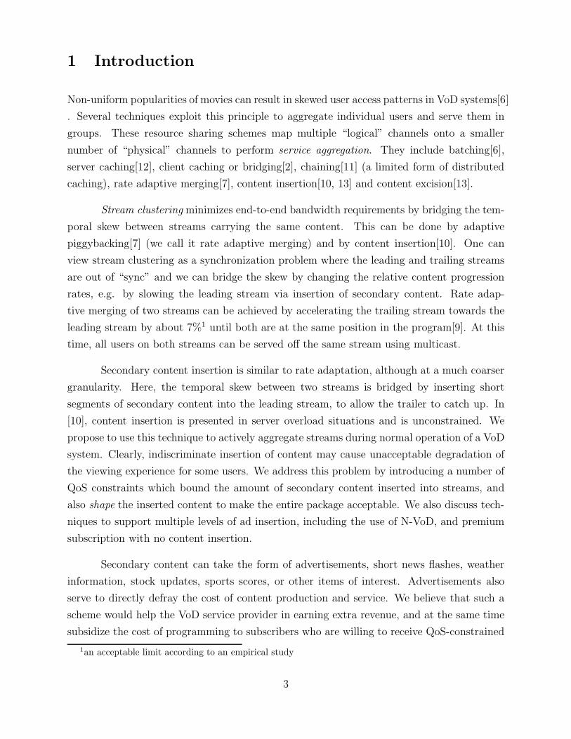
Figure 1: Ad schedule for a single user

adaptation for fine-tuning has been described in [10]. Content insertion and excision have

been discussed in conjugation with dynamic buffer management for near-VoD systems by

Tsai and Lee [13]. Optimal techniques for performing rate-adaptive merging or adaptive pig-

gybacking have been discussed in [3, 1]. An implementation of dynamic service aggregation

using rate-adaptive merging has been described in [4].

Section 2 describes the problem and the constraints in detail; Section 3 discusses a

restricted case of the problem and proposes a solution for this case; Section 4 extends this

solution to the generalized case; Section 5 touches upon some practical issues which may

be encountered during implementation. Section 6 discusses some simulation results for the

snapshot case. Section 7 concludes the paper.

2 Problem Formulation

We define an ad schedule as a sequence of tuples, of the form (aj , vj). This represents delivery

of advertisements for time aj, followed by delivery of video content for time vj . Figure 1

depicts a possible ad schedule for a single user. When generalized to a set of U users, the ad

schedule becomes a matrix of tuples (aij , vij), where each tuple represents the jth pair of ad

and video time given to user i. Typically, the interval aij will consist of a burst of multiple

ads.

If the system could insert ads in an unconstrained manner, the optimal way to merge

two users temporally separated by T seconds, is to keep the leader on ads for T seconds, and

allow the trailer to catch up in this time period. For large values of T , this unacceptably

degrades the viewing experience for the leader. Therefore, aggressive use of advertisement

scheduling can succeed only when it is controlled by a set of QoS constraints which ensure

that the viewing experience is not intolerably degraded due to advertising: no burst of ads

should be excessively long; neither should ad bursts be delivered too close to each other;

no user should receive more than a certain amount of ad time over some viewing interval;

partial ads cannot be displayed. These constraints can be formally stated as follows:

5

aij = nAmin n ∈ Z+ ∀i,j (1)

aij ≤ Amax ∀i,j (2)

vij ≥ Vmin ∀i,j (3)∑

T

aij ≤ α∑

T

(aij + vij) ∀i,j (4)

In this paper, we assume that all advertisements are of the same length, Amin which

represents the granularity of every aij. However, this approach can easily be extended to

serve ads of different lengths, as long as all the ad-lengths are integer multiples of some base

value Amin. Amax is the maximum length of a single ad burst. Clearly, Amax should also be

an integer multiple of Amin. Vmin is the minimum video time that has to occur between two

ad-bursts. There are two limits on the fraction of viewing time that can be used to display

ads. One is the long-term ad-dosage limit (α, T ), which represents the fraction of viewing

time available for ads α, over some time interval T . This is a pinwheel scheduling constraint

[8], applicable over any time interval T . The other is the short-term ad-dosage limit which

represents the maximum rate at which ads can be inserted in video. It is given by

β =Amax

Amax + Vmin

(5)

It is easy to see that in general, α ≤ β. The problem which we are trying to address

in this paper is the following:

“For a group of N streams carrying the same content but at different points in

time (i.e. if a snapshot of the stream positions is taken at a particular time

instant), what is the ad-video schedule that minimizes the total bandwidth while

merging them into one stream, at the same time obeying the above QoS con-

straints?”

If at the start of the merging cycle, stream i was at position pi and stream j was at

position pj, then for these two streams to merge, the following should hold:

pi − pj = nAmin n ∈ Z+ (6)

This implies that ad scheduling can only be used to bridge skews which are integral

multiples of the minimum ad length. In practice, such temporal skews are uncommon,

therefore ad insertion must be coupled with another, more fine-grained aggregation technique

like rate adaptive merging [7].

6

3 A Restricted Case

We first consider a restricted scenario, where ad scheduling is constrained by a number of

simplifying assumptions. In further sections, we will remove these and discuss a generalized

solution to the problem. The simplified problem has the following additional constraints:

α = β (7)

aij = 0 |Amax ∀i,j (8)

vij = Vmin ∀i,j (9)

Briefly, we simplify the problem by making the two constraints on ad dosage equal.

Also, we constrain the ad dosage to zero, or a fixed value which is the maximum we can

give. Inter-ad video dosage is also fixed at the minimum possible limit. It is clear that

any solution satisfying these constraints will also satisfy the general constraints presented

earlier. As described previously we observe an additional constraint on program positions

at the start of the merging cycle:

pi − pj = nAmax n ∈ Z+ ∀i,j (10)

Hence, the restricted problem can only merge programs whose initial difference is an

integral multiple of our ad dosage unit (Amax in this case).

3.1 Preliminaries

We first introduce a graphical notation to denote the merge-able streams with different

content progression rates on a time scale. On the left in Figure 2 is an intuitive representation

of the streams on Cartesian axes; diagonal motion along a line with slope 1 refers to a

stream with normal speed and vertical motion refers to a stream in content-insertion state.

For simplicity, we use a rectilinear representation of this graph, as shown on the right in

Figure 2. The figure has two time axes: horizontal for video time, and vertical for ad time.

Units on both these axes are taken to be equal. Note that for two streams with an initial

skew ∆ to merge, the leading stream must be given ads for ∆ time more than the trailing

stream. The leading stream is farthest to the right. Other streams are placed along the

7

Time

merge points

program position

ads

(j) (i)(k+1) (k)

3

7

9

(b) Rectilinear Representation(a) Intuitive Representation

Time

Vmin

Vmin

Amax

45o

0 3 7 9

Program Position

25

m = 0.5

Slope = -1

Amax = 1Vmin = 2

m = 1/2

P(i,j)

Vmin

Amax

(i)

(j)

(k+1)

(k)

T(i,k)

T(k+1,j)

P(k+1,j)

β = 1/3P(i,k)

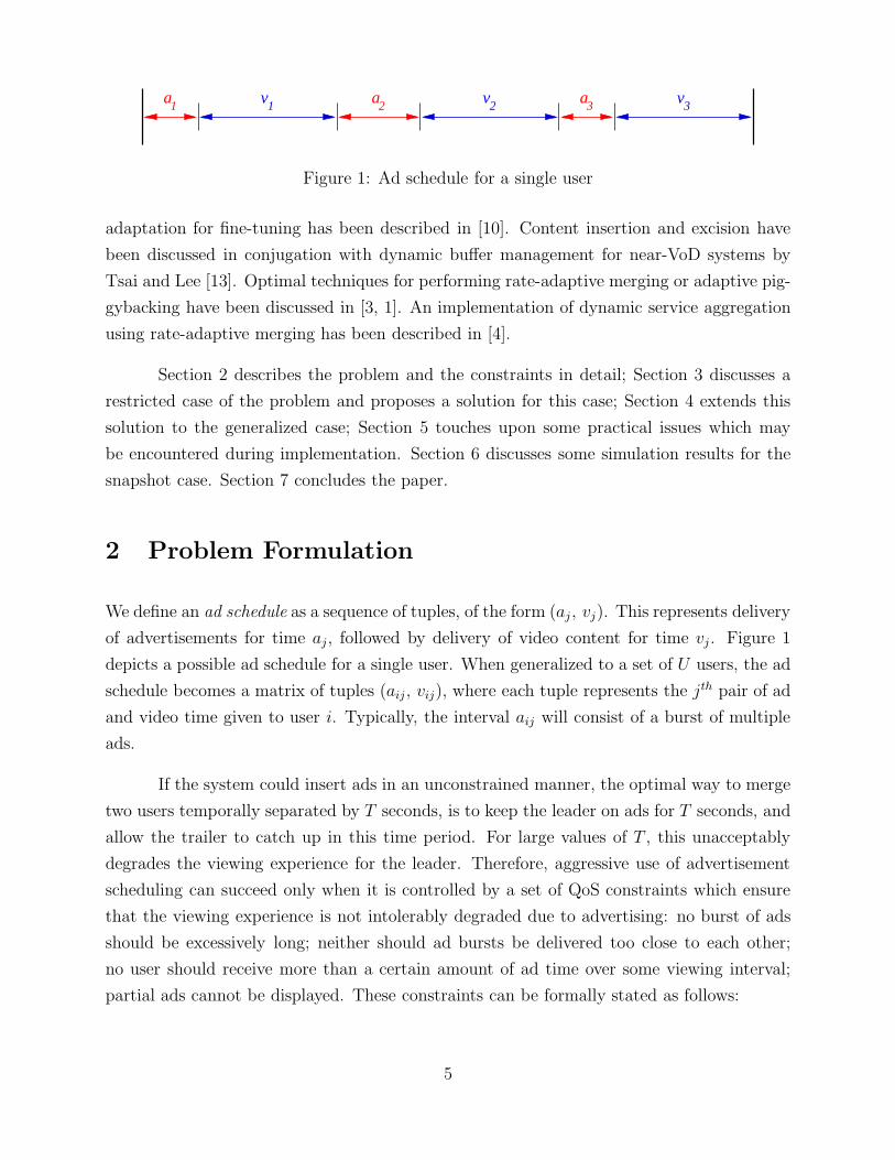
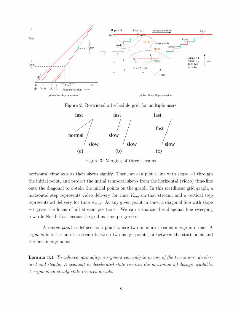
Figure 2: Restricted ad schedule grid for multiple users

(a) (b) (c)

normal

fast

slow slow

fast fast

slow

fastslow

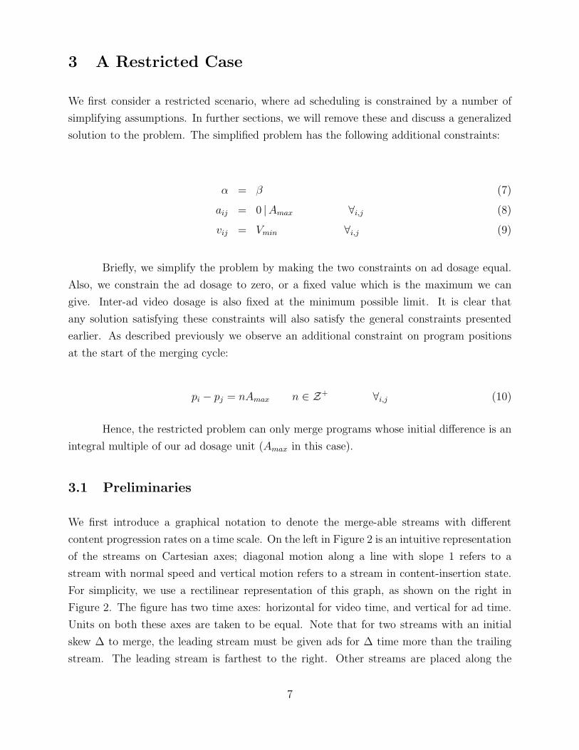
Figure 3: Merging of three streams

horizontal time axis as their skews signify. Then, we can plot a line with slope −1 through

the initial point, and project the initial temporal skews from the horizontal (video) time-line

onto the diagonal to obtain the initial points on the graph. In this rectilinear grid graph, a

horizontal step represents video delivery for time Vmin on that stream, and a vertical step

represents ad delivery for time Amax. At any given point in time, a diagonal line with slope

−1 gives the locus of all stream positions. We can visualize this diagonal line sweeping

towards North-East across the grid as time progresses.

A merge point is defined as a point where two or more streams merge into one. A

segment is a section of a stream between two merge points, or between the start point and

the first merge point.

Lemma 3.1 To achieve optimality, a segment can only be in one of the two states: deceler-

ated and steady. A segment in decelerated state receives the maximum ad-dosage available.

A segment in steady state receives no ads.

8

Lemma 3.2 At each merge point, exactly two segments merge into a single segment.

This can be deduced by noting that a segment lies between merge points, and therefore

does not contain any merge points within itself. Therefore, the aim of giving advertisements

to a stream can only be to slow it down so that a trailing stream may catch up. Since this state

of affairs will not change through the length of the segment, clearly the optimal scheduling

policy will decelerate the segment at the maximum possible rate. This is illustrated in Figure

3. It is clear that both case (b) and case (c) have less cost than case (a).

Lemma 3.3 If advertisements are to be inserted in a segment, it is less costly to give ad-

vertisements as early as possible, and video content later.

If the decelerated stream is not going to merge with any stream within the current

ad-video pair, then it does not matter. However, if the decelerated stream is merging with a

trailing stream within this ad-video pair, optimal use of bandwidth is achieved by having ads

as early as possible. In Figure 4(a), the decelerated stream merges earlier with the trailing

stream than in 4(b), because ads are given earlier. This lemma is central to many of the

proofs in this paper.

Lemma 3.4 For a decelerated segment, the optimal ad scheduling technique is to give the

maximum possible ad dosage in the beginning, followed by the video complement for this ad

dosage. This pattern is repeated periodically throughout the segment.

This follows from Lemma 3.3 and the pinwheel scheduling constraint in Equation

4. So as not to violate the pinwheel scheduling requirement, we must give a periodic ad-

video-pairing, with each period satisfying the scheduling requirement. A notable exception

to this lemma occurs when giving ads early violates some other constraint. For example,

immediately before a merge point, the decelerated stream receives an ad burst. Therefore,

immediately after the merge point, the merged segment must receive a video burst; otherwise,

the viewers of the prior decelerated stream receive too many ads.

Lemma 3.5 The point where all streams finally merge occurs at a time Vmin before the

intersection of a horizontal line drawn from the trailing stream, and a diagonal line of slope

m = β

1−βdrawn from the leading stream. All streams are constrained within the envelope

formed by these two lines.

9

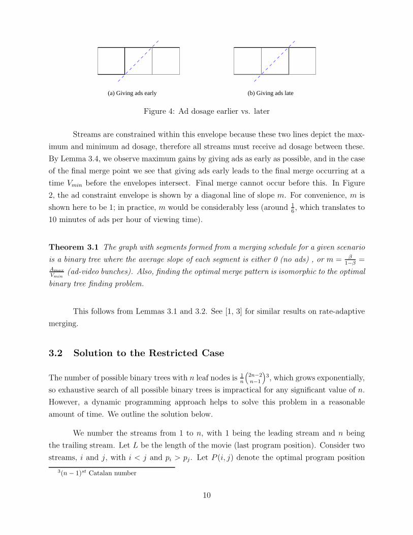
(a) Giving ads early (b) Giving ads late

Figure 4: Ad dosage earlier vs. later

Streams are constrained within this envelope because these two lines depict the max-

imum and minimum ad dosage, therefore all streams must receive ad dosage between these.

By Lemma 3.4, we observe maximum gains by giving ads as early as possible, and in the case

of the final merge point we see that giving ads early leads to the final merge occurring at a

time Vmin before the envelopes intersect. Final merge cannot occur before this. In Figure

2, the ad constraint envelope is shown by a diagonal line of slope m. For convenience, m is

shown here to be 1; in practice, m would be considerably less (around 1

6, which translates to

10 minutes of ads per hour of viewing time).

Theorem 3.1 The graph with segments formed from a merging schedule for a given scenario

is a binary tree where the average slope of each segment is either 0 (no ads) , or m = β

1−β=

Amax

Vmin(ad-video bunches). Also, finding the optimal merge pattern is isomorphic to the optimal

binary tree finding problem.

This follows from Lemmas 3.1 and 3.2. See [1, 3] for similar results on rate-adaptive

merging.

3.2 Solution to the Restricted Case

The number of possible binary trees with n leaf nodes is 1

n

(

2n−2

n−1

)

3, which grows exponentially,

so exhaustive search of all possible binary trees is impractical for any significant value of n.

However, a dynamic programming approach helps to solve this problem in a reasonable

amount of time. We outline the solution below.

We number the streams from 1 to n, with 1 being the leading stream and n being

the trailing stream. Let L be the length of the movie (last program position). Consider two

streams, i and j, with i < j and pi > pj . Let P (i, j) denote the optimal program position

3(n − 1)st Catalan number

10

where streams i and j would merge, if these were the only two streams under consideration.

This is well-defined from Lemma 3.5 as a point which is Vmin time before the intersection

of a horizontal line through j and a line of slope m = β

1−βthrough i. If we now consider

the streams i, . . . , j, then an optimal merge policy cannot merge these streams earlier than

P (i, j). Also, it is easy to see that the existence of other streams in the range i, . . . , j cannot

prevent i and j from merging at P (i, j). Therefore, P (i, j) is the optimal final merge point

for streams i, . . . , j and is given by:

P (i, j) = pi, i = j (11)

= pj +pi − pj

β− Vmin, i 6= j (12)

Let T (i, j) denote an optimal binary tree for merging streams i, . . . , j. Let C(i, j)

denotes the cost of this tree. Since this is a binary tree, there exists a point k such that the

right subtree contains the nodes i, . . . , k and the left subtree contains the nodes k +1, . . . , j.

From the principle of optimality, if T (i, j) is optimal (has minimum cost) then both the left

and right subtrees must be optimal. That is, the right and left subtrees of T (i, j) must be

T (i, k) and T (k + 1, j). The cost of this tree is given by

C(i, j) = L − pi, i = j (13)

= C(i, k) + C(k + 1, j) − max(L − P (i, j), 0) + (pk − pj), i 6= j (14)

and the optimal policy merges T (i, k∗) and T (k∗ +1, j) into T (i, j), where k∗ is given

by

k∗ = argmini≤k<j{C(i, k) + C(k + 1, j) − max(L − P (i, j), 0) + (pk − pj)} (15)

Here C(i, k) and C(k+1, j) are the costs of the right and the left subtrees respectively,

calculated all the way till the end of the movie. The third term is subtracted to eliminate

the cost duplication after the streams i and j merge. The fourth term is added to figure in

the ad time after P (i, k) into the cost formulation. This is because, even if a certain stream

has been put on ads momentarily, the resources allocated to it in the server and the network

(in case of bandwidth reservation) cannot be freed until it actually merges with some other

11

stream. Since the number of ad channels is assumed to be fixed (ideally, one multicast ad

channel suffices), the bandwidth costs due to those channels do not feature in Equation 14.

We begin by calculating T (i, i) and C(i, i) for all i. Then, we calculate T (i, i+1) and

C(i, i + 1), then T (i, i + 2) and C(i, i + 2) and so on, until we find T (1, n) and C(1, n). This

gives us our optimal cost. The algorithm can be summarized as follows:

Algorithm DP Find Tree{

for (i=1 to n)initialize P (i, i), C(i, i) and T (i, i) from equations 11 and 13

for (p=1 to n − 1)for (q=1 to n − p)Compute P (q, q + p), C(q, q + p) and T (q, q + p) from equations 12, 14 and 15

}

There are O(n) iterations of the outer loop and O(n) iterations of the inner loop.

Additionally, determination of C(i, j) requires O(n) comparisons in the argmin step. Hence,

the algorithm DP Find Tree has a complexity of O(n3). A point to be noted here is that

in real systems, n is not likely to be very high, thus making the complexity acceptable. We

show later in the simulation section that not much optimality is lost by reducing the size of

a snapshot.

4 The General Case

In this section, we attempt to solve the scheduling problem for more general cases by relaxing

the constraints imposed in the previous section.

4.1 First-Stage Constraint Relaxation

We begin by relaxing the constraints outlined in Equation 8. Therefore, aij is now variable,

subject to equations 1 and 2. The graphical representation of this case is shown in Figure 5.

From lemma 3.3, the optimal scheduling policy schedules as much ad time as early

as possible, and then fills in the video as necessary. We can easily see that the problem

12

Vmin

A max

A min

Video Time

Ad T

ime

i

slope=m

k

k+1

j

l

Snapshot

P’

P(i, j)P

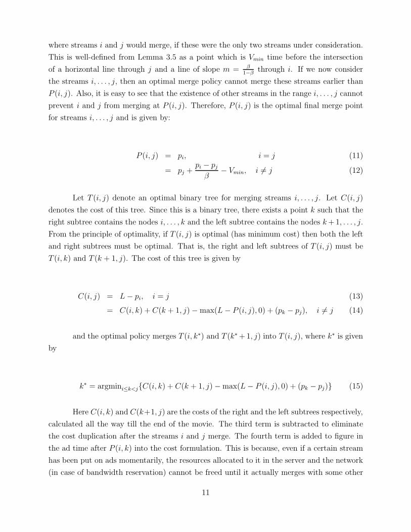
Figure 5: First-stage constraint relaxation

once again reduces to an optimal binary tree problem. In this case, calculation of P (i, j) is

different from the previous one since a merge point can occur during an ad-burst. It is given

by:

P (i, j) = pi + (dpi − pj

Amax

e − 1) × Vmin, (16)

where dpi−pj

Amaxe − 1 is the number of times ads are given till point P’ on the tree.

Multiplying this quantity by Vmin yields the amount of video given till point P, since no

video is given between P’ and P. To represent the tree T (i, j) completely, we also need to

store at each merge point the additional amount of ads that can be given to that stream

without violating any constraints. We represent this by SAgo and it is given by,

SAgo(i, j) = Amax − (pi − pj) mod Amax (17)

Since we can accurately determine P (i, j) for any i, j using Equation 16, we can

use algorithm DP Find Tree to find an optimal tree for this generalized case, substituting

equation 16 in place of equation 12. Further, since the complexity of determining P (i, j) is

O(1), the complexity of this algorithm remains O(n3).

13

Amax

Amin

i

T-T’

slope=q

slope=p

kVmin

T’

j

k+1

i

Snapshot

P(i, j)

P’

P

O

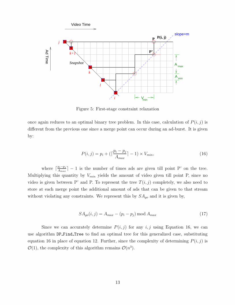
Figure 6: Second-stage constraint relaxation

4.2 Further Relaxation of Constraints

We complete the generalization by relaxing the final artificial constraint, given in equation

7. Now we have to handle two ad constraints, the short-term constraint and the long-term

constraint. The short-term ad constraint, defined in Equation 5, is represented on the grid

graph by a line of slope p, where p = β

1−β. The long-term ad constraint (α, T ) is represented

on the graph by a line of slope q, where q = α1−α

.

These constraints are depicted in figure 6 where we attempt to calculate P (i, j) by

considering the subtrees T (i, k) and T (k + 1, j). Through i, we draw two diagonal lines of

slopes p and q. Initially, the decelerated segment follows line p as specified in section 4.1.

However, now the long-term constraint is also in force. Therefore, the scheduler must ensure

that after time T , segment OP has an average slope q. This can be enforced by the following

technique. We know that T ′ = αT is the maximum ad-dosage possible within time interval

T . Therefore, the scheduler keeps track of how much ad-dosage has been given within this

long-term interval T . If the ad-dosage given is T ′, then the scheduler will not give any more

ads for the remaining time in interval T . Once time interval T has elapsed, the scheduler

once again begins inserting ads at an average rate p.

Again in this case, P (i, j) has to be calculated in a slightly different manner:

P (i, j) = pi + (d(pi − pj)

T ′e − 1) × (T − T ′) + (d

MOD(pi − pj , T′)

Amax

e − 1) × Vmin(18)

MOD(x, k) = 1 + (x − 1)mod k (19)

14

The second additive term corresponds to the video given in the segment OP ′ and the

third term amounts to the video given in the segment P ′P . Each merge point stores SAgo,

representing the ad-time remaining in the current burst, and LAgo, representing the ad-time

remaining in this current long-term section. The equations for these quantities can be found

out using logic similar to that used in Equations 17 and 18, and have been omitted due to

paucity of space. Note that if pi − pj < T ′, then this merge can be scheduled by the rules in

section 4.1.

Since we can obtain P (i, j) accurately, once again the algorithm DP Find Tree can

be used to generate the optimal merging schedule. Furthermore, since evaluation of P (i, j)

is an O(1) operation, the complexity of the algorithm remains O(n3). This analysis is valid

only for static snapshots; changing scenarios due to user interactions are discussed in the

next section. In the above analysis, we also assume that the counters SAgo and LAgo have

been reset to Amax and T ′ respectively at the beginning of the snapshot. One way to ensure

this is to run all the streams at a steady state for some time t, such that the ad-counters

are reset. Essentially t will be the maximum of the long-run “to-go” video time over all

streams. Clearly t ≤ T ′. But running all the streams at steady state for time t can be a

source of suboptimality in dynamic situations, hence we require schemes that do not need

the ad-counters to be reset. We discuss one such scheme in the following subsection.

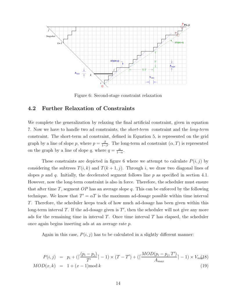
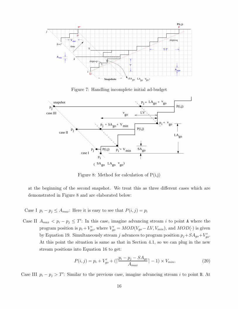
4.3 Optimal Scheduling with Incomplete Initial Ad-Budget

In this case, a starting stream i is characterized by a program position pi and a triplet

(SAgo, LAgo, Vgo). SAgo is the remaining short-term ad budget as described previously, LAgo

is the long-term ad budget which can be calculated similarly, and Vgo is the remaining amount

of video that has to be given to this stream in the current long-term period. Whenever a

stream enters the system or goes through a long-term period of time T , this triplet is set

to (Amax, T′, T − T ′). In order to calculate the new optimal paths for streams with triplet

constraints from a current snapshot, we need to modify the equations 16 and 18. The

situation has been represented in Figure 7 at the second snapshot. Stream i has a triplet

constraint associated with it. Lemma 3.4 instructs the scheduler to give all the remaining ads

(SAgo) right-away, followed by periodic ad-video bursts. So essentially the leading stream

keeps on running the way it was.

Now, we will derive the modified expressions for P (i, j) for all pairs of streams (i, j)

in this scenario. Let pi, pj be the positions of the leading and trailing streams respectively,

15

XXXXXXXX

S

(SAgo LAgo Vgo )

time

Amax

Vmin

Amin

P(i, j)

P

Oi

k+1

j

k

Snapshots

T’

T-T’

slope=q

slope=p

P’’

P’

Figure 7: Handling incomplete initial ad-budget

pi

pj

pj

pj

pj

pi

pi

pj

goSA Vmin

Vmin

gov

goLA

gov

goSA goLA gov

goSA

goLA

gov

+ +

+

+ +

+

P(i,j)

P(i,j)

P(i,j)

( )

snapshot

case II

case III

case I

LV

Figure 8: Method for calculation of P(i,j)

at the beginning of the second snapshot. We treat this as three different cases which are

demonstrated in Figure 8 and are elaborated below:

Case I pi − pj ≤ Amax: Here it is easy to see that P (i, j) = pi

Case II Amax < pi − pj ≤ T ′: In this case, imagine advancing stream i to point A where the

program position is pi +V ′go, where V ′

go = MOD(Vgo−LV, Vmin), and MOD(·) is given

by Equation 19. Simultaneously stream j advances to program position pj +SAgo+V ′go.

At this point the situation is same as that in Section 4.1, so we can plug in the new

stream positions into Equation 16 to get:

P (i, j) = pi + V ′go + (d

pi − pj − SAgo

Amax

e − 1) × Vmin, (20)

Case III pi − pj > T ′: Similar to the previous case, imagine advancing stream i to point B. At

16

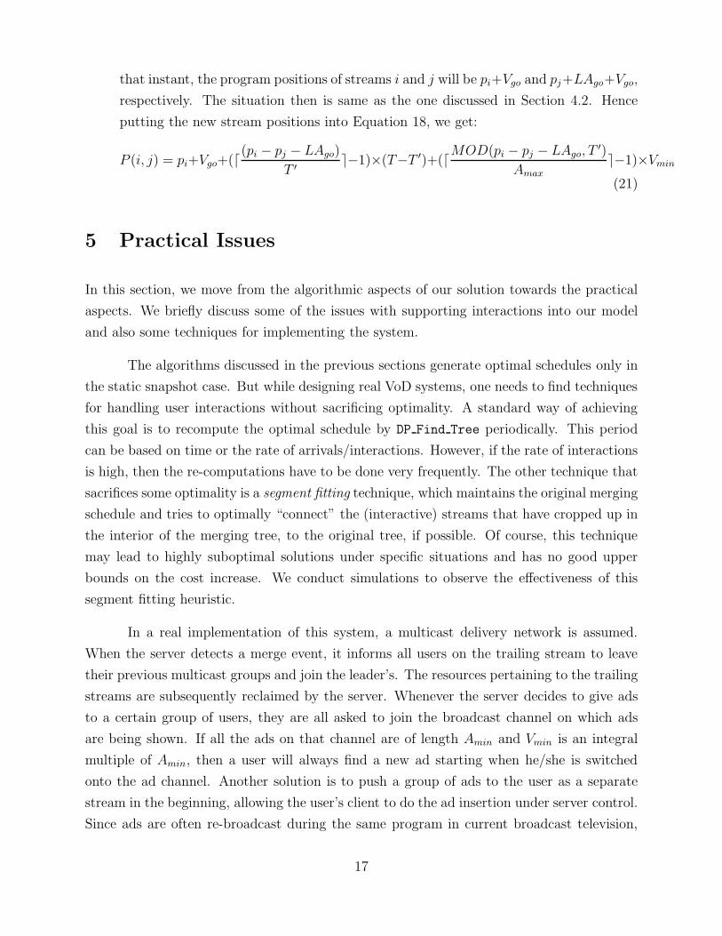
that instant, the program positions of streams i and j will be pi+Vgo and pj+LAgo+Vgo,

respectively. The situation then is same as the one discussed in Section 4.2. Hence

putting the new stream positions into Equation 18, we get:

P (i, j) = pi+Vgo+(d(pi − pj − LAgo)

T ′e−1)×(T−T ′)+(d

MOD(pi − pj − LAgo, T′)

Amax

e−1)×Vmin

(21)

5 Practical Issues

In this section, we move from the algorithmic aspects of our solution towards the practical

aspects. We briefly discuss some of the issues with supporting interactions into our model

and also some techniques for implementing the system.

The algorithms discussed in the previous sections generate optimal schedules only in

the static snapshot case. But while designing real VoD systems, one needs to find techniques

for handling user interactions without sacrificing optimality. A standard way of achieving

this goal is to recompute the optimal schedule by DP Find Tree periodically. This period

can be based on time or the rate of arrivals/interactions. However, if the rate of interactions

is high, then the re-computations have to be done very frequently. The other technique that

sacrifices some optimality is a segment fitting technique, which maintains the original merging

schedule and tries to optimally “connect” the (interactive) streams that have cropped up in

the interior of the merging tree, to the original tree, if possible. Of course, this technique

may lead to highly suboptimal solutions under specific situations and has no good upper

bounds on the cost increase. We conduct simulations to observe the effectiveness of this

segment fitting heuristic.

In a real implementation of this system, a multicast delivery network is assumed.

When the server detects a merge event, it informs all users on the trailing stream to leave

their previous multicast groups and join the leader’s. The resources pertaining to the trailing

streams are subsequently reclaimed by the server. Whenever the server decides to give ads

to a certain group of users, they are all asked to join the broadcast channel on which ads

are being shown. If all the ads on that channel are of length Amin and Vmin is an integral

multiple of Amin, then a user will always find a new ad starting when he/she is switched

onto the ad channel. Another solution is to push a group of ads to the user as a separate

stream in the beginning, allowing the user’s client to do the ad insertion under server control.

Since ads are often re-broadcast during the same program in current broadcast television,

17

this technique can save network bandwidth by rotating ads in the client.

Personalization and value-added secondary content such as news are important factors

in increasing the acceptability of this solution. For example, we may have four multicast

ad channels, one multicast news channel, one multicast sports channel, and so on. These

channels may show the same content in one-minute bursts, for half an hour. By appropriately

switching the leader to different multicast channels, we can improve his overall viewing

experience. Further, the ad channels may be personalized to groups of target customers.

Preloading ads to the client as discussed above could also be leveraged for personalization.

Another important factor for the success of ad insertion is an appropriate pricing

policy. Inserting ads in this manner has the dual benefit of reducing server requirements

by aggregating users, and providing a revenue stream to content and service providers.

Any pricing structure has to provide enough subsidies to the user to make an ad-inserted

package attractive to him/her. On the other hand, users interacting heavily during ads and

video should be made to pay the price. Also, uniform ad insertion into a video stream

is not always feasible due to the occurrence of “gripping” situations. We propose off-line

insertion of certain metadata into the stream which will instruct the server not to attempt

any aggregation at that point in time.

6 Simulation Results

In this section, we describe the simulation experiments that we designed for evaluating the

gains due to secondary content insertion. We report the results for the snapshot case in the

next subsection. The simulation procedure and results for the dynamic case are presented

in Section 6.2.

6.1 Snapshot Case Results

In this section we present the simulation results for the most general case of the content

insertion algorithm presented in Section 4. We assume a static snapshot of the program

positions of all users and try to merge them using our algorithm. Table 1 enlists the various

parameters used in the simulations.

For simulating a static snapshot, we generate exponentially distributed program po-

sitions separated by mean time interval 1

λ. Then we try to merge the streams using two

18

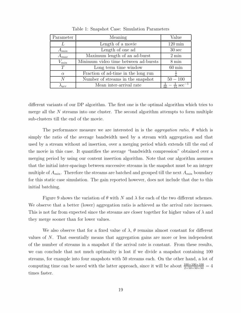
Table 1: Snapshot Case: Simulation Parameters

Parameter Meaning Value

L Length of a movie 120 minAmin Length of one ad 30 secAmax Maximum length of an ad-burst 2 minVmin Minimum video time between ad-bursts 8 minT Long term time window 60 minα Fraction of ad-time in the long run 1

6

N Number of streams in the snapshot 50 − 100λarr Mean inter-arrival rate 1

60− 1

15sec−1

different variants of our DP algorithm. The first one is the optimal algorithm which tries to

merge all the N streams into one cluster. The second algorithm attempts to form multiple

sub-clusters till the end of the movie.

The performance measure we are interested in is the aggregation ratio, θ which is

simply the ratio of the average bandwidth used by a stream with aggregation and that

used by a stream without ad insertion, over a merging period which extends till the end of

the movie in this case. It quantifies the average “bandwidth compression” obtained over a

merging period by using our content insertion algorithm. Note that our algorithm assumes

that the initial inter-spacings between successive streams in the snapshot must be an integer

multiple of Amin. Therefore the streams are batched and grouped till the next Amin boundary

for this static case simulation. The gain reported however, does not include that due to this

initial batching.

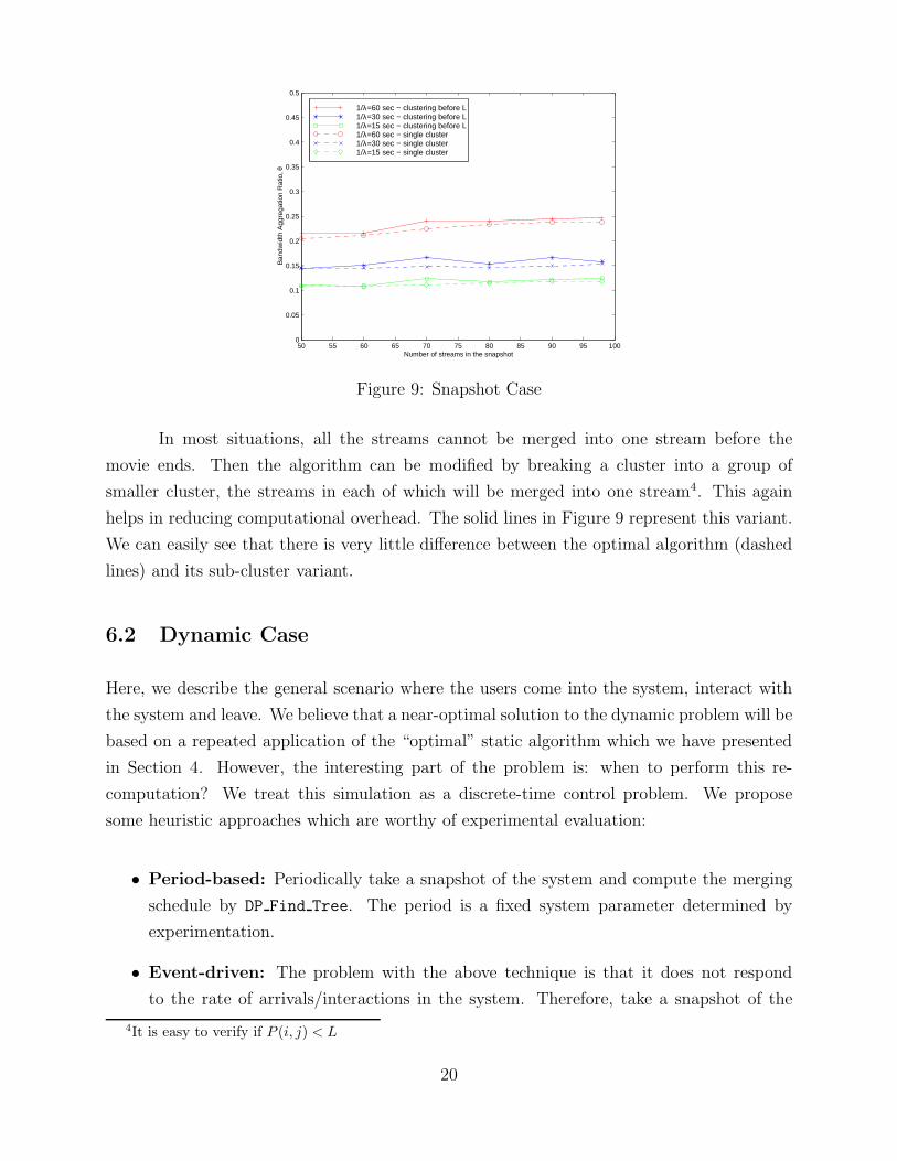
Figure 9 shows the variation of θ with N and λ for each of the two different schemes.

We observe that a better (lower) aggregation ratio is achieved as the arrival rate increases.

This is not far from expected since the streams are closer together for higher values of λ and

they merge sooner than for lower values.

We also observe that for a fixed value of λ, θ remains almost constant for different

values of N . That essentially means that aggregation gains are more or less independent

of the number of streams in a snapshot if the arrival rate is constant. From these results,

we can conclude that not much optimality is lost if we divide a snapshot containing 100

streams, for example into four snapshots with 50 streams each. On the other hand, a lot of

computing time can be saved with the latter approach, since it will be about 100×100×100

2×50×50×50= 4

times faster.

19

50 55 60 65 70 75 80 85 90 95 1000

0.05

0.1

0.15

0.2

0.25

0.3

0.35

0.4

0.45

0.5

Number of streams in the snapshot

Ban

dwid

th A

ggre

gatio

n R

atio

, θ

1/λ=60 sec − clustering before L1/λ=30 sec − clustering before L1/λ=15 sec − clustering before L1/λ=60 sec − single cluster 1/λ=30 sec − single cluster 1/λ=15 sec − single cluster

Figure 9: Snapshot Case

In most situations, all the streams cannot be merged into one stream before the

movie ends. Then the algorithm can be modified by breaking a cluster into a group of

smaller cluster, the streams in each of which will be merged into one stream4. This again

helps in reducing computational overhead. The solid lines in Figure 9 represent this variant.

We can easily see that there is very little difference between the optimal algorithm (dashed

lines) and its sub-cluster variant.

6.2 Dynamic Case

Here, we describe the general scenario where the users come into the system, interact with

the system and leave. We believe that a near-optimal solution to the dynamic problem will be

based on a repeated application of the “optimal” static algorithm which we have presented

in Section 4. However, the interesting part of the problem is: when to perform this re-

computation? We treat this simulation as a discrete-time control problem. We propose

some heuristic approaches which are worthy of experimental evaluation:

• Period-based: Periodically take a snapshot of the system and compute the merging

schedule by DP Find Tree. The period is a fixed system parameter determined by

experimentation.

• Event-driven: The problem with the above technique is that it does not respond

to the rate of arrivals/interactions in the system. Therefore, take a snapshot of the

4It is easy to verify if P (i, j) < L

20

system whenever the number of new arrivals or interactions exceeds a given threshold.

As a refinement the count can be on a per-movie basis, that is, recompute for that

movie if the number of arrivals and interactions exceeds a threshold. Recomputing on

every event may lead to sub-optimal results. Again, the threshold parameter has to be

determined experimentally.

• Adaptive: Adapt the re-computation period based on interactivity and the state of

the system. For example, for high degrees of interaction, the re-computation period

should be small, and vice-versa.

• Policy iteration: Based on observed system behavior over a large period of time,

compute the best policy for each set of circumstances. Choose the best policy for the

current circumstance.

• Customer Profiling: Some customers may be highly interactive, whereas others may

be relatively passive. If we can trace a customer’s profile from the logs, we can decide

whether to keep him/her on a separate stream (if he/she interacts often) or to include

him/her in a current snapshot. Accurate profiling may result in near-optimal solutions.

The set up consists of two logical modules: a discrete event simulation driver and a

content insertion (CI) unit. The simulation driver maintains the state of all streams and

generates events for user arrivals, departures and VCR actions (fast-forward, rewind, pause

and quit) with inter-event times obeying a given probability distribution. A re-computation

period is an interval of time during which a content insertion algorithm attempts to release

channels. Once in every re-computation period, the simulation driver conveys the position

and status of each stream to the CI unit (which computes the merging schedule) and queries

it after every simulation tick to get the status of the streams. It then advances each stream

accordingly. For instance, if the clustering unit reports that a particular stream is to remain

in the content insertion state for a particular amount of time, the simulation driver keeps the

stream on secondary content for that time. If any customer interacts, then the simulation

driver changes the state of the corresponding stream or allocates a new one if necessary.

This experimental set up will help us evaluate all the control heuristics under different

dynamic situations, and will help us verify how much of the gain due to ad insertion in the

static case holds for the dynamic case.

In this work, we investigate the period based re-computation strategy, which is the

simplest and the easiest to implement. The main performance measure that we are interested

21

Table 2: Dynamic Case: Additional Simulation Parameters

Parameter Meaning Value

M Number of movies 100R Re-computation interval 1200 sec

B Initial batching interval Amin = 30 sec

λarr Mean inter-arrival rate 0.0833 sec−1

λint Mean interaction rate 0.07 sec−1

λdur Mean interaction duration 5 secf Rate of Rewind/FF 5x

in, in the dynamic scenario is the ratio of the number of running streams to the number of

users in the system, which directly quantifies the gains due to secondary content insertion.

We outline the dynamic simulation scheme in Figure 10.

R is the re-computation window after which a new snapshot is taken. Initially all

streams are run for time R at normal speed and only then the ad-insertion starts. At

the beginning of every snapshot, algorithm DP Find Tree computes the optimal paths for

each stream and stores them in local data structures. Until the next snapshot happens, all

currently running (non-interacting) streams follow the paths as prescribed by the algorithm.

Newly arrived streams, however are allowed to run at normal speed until the next snapshot.

One important assumption that we make in the interaction model is that interactions are

not allowed during ad-bursts. All interactions that occur during an ad-burst are serviced

at the end of the burst. When a user interacts, he/she is allocated a new stream at least

for the duration of interaction. But after resuming the user can be merged with any other

stream since the ad-budget of that stream is reset after the interaction event. This is to

discourage users from interacting for the sole purpose of skipping the ads. However, if a user

has premium service, he/she should not be affected by this.

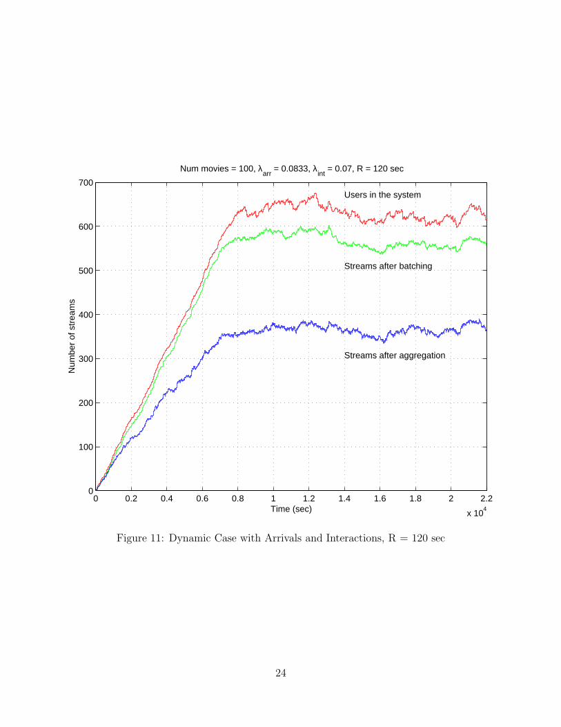
The additional simulation parameters for the dynamic case can be found in Table 2.

We simulate the case where the most popular movie has arrivals once every minute which

translates to the aggregate arrival rate of 1

12sec−1 for 100 movies. Figures 11 and 12 show the

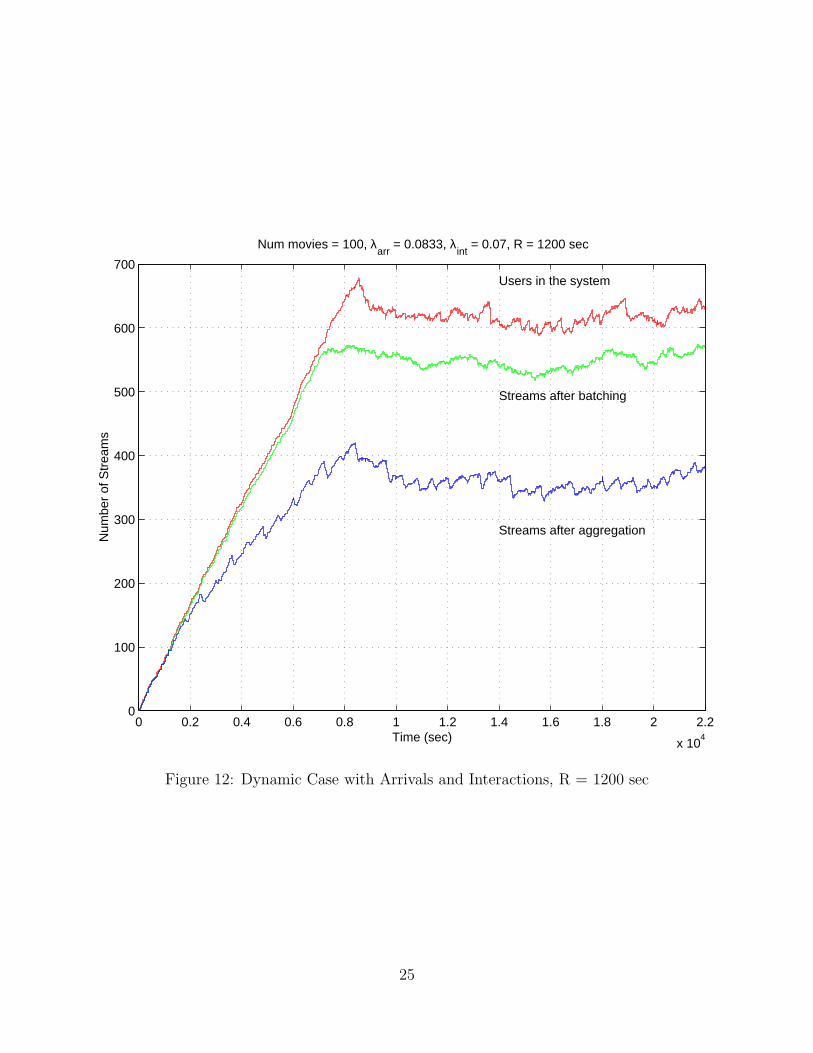
gains due to ad-insertion in this dynamic interactive scenario. The average number of users

in the system U should approximately be λarr ×L = 600, in our case. The simulations show

a slightly higher value (around 625) since ad-insertion slows users down resulting in more

number of users. But, after aggregation, the number of streams in the system is only around

350, which directly translates to a 45% saving in capacity. Therefore secondary content

insertion helps us in cutting down the bandwidth requirement to almost half the original

22

Initialize a subscriber pool, P

timecurrent = timeprev = 0;while (timecurrent < MAXSIMTIME) {

Generate movie requests from users in P ; The movies are selected from a list of M

movies according to a Zipfian popularity distribution. The inter-arrival times areexponentially distributed;

Batch the requests till the nearest Amin boundary to make the streams fall on thediscrete grid;

Generate VCR actions (FF, Rewind, Pause, Quit) and handle them;

if (timecurrent − timeprev == R)

Call algorithm DP Find Tree with the current snapshot of stream positions;Form multiple sub-clusters keeping in mind the end of the movie.Advance all streams accordingly;

timeprev = timecurrent;

else if (timecurrent < R)

Advance all streams normally with no ad-insertion;

else /* timecurrent − timeprev < R */

Advance all streams as instructed by DP Find Tree;

timecurrent + +;

}

Figure 10: Simulation Algorithm

23

0 0.2 0.4 0.6 0.8 1 1.2 1.4 1.6 1.8 2 2.2

x 104

0

100

200

300

400

500

600

700

Num movies = 100, λarr

= 0.0833, λint

= 0.07, R = 120 sec

Time (sec)

Num

ber

of s

trea

ms

Users in the system

Streams after batching

Streams after aggregation

Figure 11: Dynamic Case with Arrivals and Interactions, R = 120 sec

24

0 0.2 0.4 0.6 0.8 1 1.2 1.4 1.6 1.8 2 2.2

x 104

0

100

200

300

400

500

600

700

Num movies = 100, λarr

= 0.0833, λint

= 0.07, R = 1200 sec

Num

ber

of S

trea

ms

Time (sec)

Users in the system

Streams after batching

Streams after aggregation

Figure 12: Dynamic Case with Arrivals and Interactions, R = 1200 sec

25

amount; the spare bandwidth, if any can be used to serve a larger number of customers.

Figures 11 and 12 also show the effect of increasing the re-computation interval and

using segment fitting heuristics. R was increased from 120 seconds (fig 11) to 1200 seconds

(fig 12). We observed no appreciable increase in resource usage. This shows that for low to

medium interaction levels, segment fitting heuristics work well and re-computation can be

done relatively infrequently. This reduces the computational overhead of the algorithm.

7 Conclusions and Future Work

In this paper, we presented and evaluated an optimal algorithm for scheduling secondary

content in video-on-demand systems. We demonstrated that the algorithm runs in O(n3)

time, where n is the number of streams in a cluster. For a static snapshot of 50 − 100 users

separated with a mean inter-spacing of 1 min, we have shown a bandwidth compression by

about a factor between 4 and 5. This algorithm is well-suited for performing the merging step

in a dynamic service aggregation system. We have also presented the simulation results for a

fully interactive scenario where the users are arriving, interacting and leaving the system. For

a mean arrival rate of around 1

12sec−1, and a combined interaction rate of around 0.07sec−1,

we show almost 50% reduction in the number of channels required.

The general problem of multiple levels of differentiated content insertion needs to be

examined. Analysis of the effect of changing access patterns and interaction rates on the

performance of our algorithm is currently underway. Finally, a real prototype demonstrating

constraint ad-insertion needs to be developed for exploring some systems issues which have

been abstracted out in this modeling phase.

References

[1] C.C. Aggarwal, J.L. Wolf and P.S. Yu, “On Optimal Piggyback Merging Policies for

Video-on-Demand Systems,” Proc. SIGMETRICS ’96: Conference on Measurement

and Modeling of Computer Systems, Philadelphia, PA, USA, pp. 200-209, May 1996.

[2] K.C. Almeroth and M.H. Ammar, “On the Use of Multicast Delivery to Provide a

Scalable and Interactive Video-on-Demand Service,” IEEE Journal on Selected Areas

in Communication, Vol. 14, No. 6, pp. 1110-1122, Aug 1996.

26

[3] P. Basu, R. Krishnan, T.D.C. Little, “Optimal Stream Clustering Problems in Video-on-

Demand,” Proc. Parallel and Distributed Computing and Systems ’98 - Special Session

on Distributed Multimedia Computing, Las Vegas, NV, USA, pp. 220-225, Oct 1998.

[4] P. Basu, A. Narayanan, R. Krishnan and T.D.C. Little, “An Implementation of Dynamic

Service Aggregation for Interactive Video Delivery,” Proc. SPIE Multimedia Computing

and Networking ’98, San Jose, CA, USA, pp. 110-122, Jan 1998.

[5] P. Basu, A. Narayanan, W. Ke, T.D.C. Little and A. Bestavros, “Schedul-

ing of Secondary Content for Aggregation in Commercial Video-on-

Demand Systems,” MCL Technical Report MCL-TR-12-16-98, Dec 1998.

URL: http://hulk.bu.edu/pubs/papers/1999/basu-adins99/TR-12-16-98.ps.gz

[6] A. Dan, D. Sitaram, and P. Shahabuddin, “Scheduling Policies for an On-Demand Video

Server with Batching,” Proc. ACM Multimedia, San Francisco, CA, USA, pp. 15-23, Oct

1994.

[7] L. Golubchik, J.C.S. Lui and R.R. Muntz, “Adaptive Piggybacking: A Novel Tech-

nique for Data Sharing in Video-On-Demand Storage Servers,” Multimedia Systems,

ACM/Springer-Verlag, Vol. 4, pp. 140-155, 1996.

[8] R. Holte et al., “The pinwheel: A real-time scheduling problem” Proc. 22nd Hawaii

International Conference on System Science pp 693-702, Kailua-Kona, HI, USA, Jan

1989.

[9] R. Krishnan and T. D. C. Little, “Service Aggregation Through a Novel Rate Adaptation

Technique Using a Single Storage Format,” Proc. 7th Intl. Workshop on Network and

Operating System Support for Digital Audio and Video, St. Louis, MO, USA, May 1997.

[10] R. Krishnan, D. Ventakesh and T.D.C. Little, “A Failure and Overload Tolerance Mech-

anism for Continuous Media Servers,” Proc. Fifth Intl. ACM Multimedia Conference,

Seattle, WA, USA, pp. 131-142, Nov 1997.

[11] S. Sheu and K.A. Hua, “Virtual batching: A new scheduling technique for video-on-

demand servers,” Fifth International Conference on Database Systems for Advanced

Applications, Melbourne, Australia, Apr 1997.

[12] W.D. Sincoskie, “System Architecture for a Large Scale Video on Demand Service,”

Computer Networks and ISDN systems, Vol. 22, pp. 155-162, 1991.

27

[13] W.-J. Tsai and S.-Y. Lee, “Dynamic Buffer Management for Near Video-On-Demand

Systems,” Multimedia Tools and Applications, Kluwer Academic Publishers, Vol. 6 Issue

1, pp. 61-83, Jan 1998.

28