Optimal Selection of Classification Algorithms for Well Log Interpretation

- 37 - http://www.sj-ce.org

ScientificJournalofControlEngineeringJune2015,Volume5,Issue3,PP.37‐50

Optimal Selection of Classification Algorithms for Well Log Interpretation Guangren Shi†, Jinshan Ma, Dan Ba

Research Institute of Petroleum Exploration and Development, PetroChina, P. O. Box 910, Beijing 100083, China †Email: [email protected]

Abstract

Three classification algorithms and one regression algorithm have been applied to well log interpretation. The three classification

algorithms are the classification of support vector machine (C-SVM), the naïve Bayesian (NBAY), and the Bayesian successive

discrimination (BAYSD), while the one regression algorithm is the multiple regression analysis (MRA). In these four algorithms,

only MRA is a linear algorithm whereas the other three are nonlinear algorithms. In general, when all these four algorithms are

used to solve a real-world problem, they often produce different solution accuracies. Toward this issue, the solution accuracy is

expressed with the total mean absolute relative residual for all samples, R(%). Then three criteria have been proposed: 1)

nonlinearity degree of a studied problem based on R(%) of MRA (weak if R(%)<10, and strong if R(%)≥10); 2) solution accuracy

of a given algorithm application based on its R(%) (high if R(%)<10, and low if R(%)≥10); and 3) results availability of a given

algorithm application based on its R(%) (applicable if R(%)<10, and inapplicable if R(%)≥10). Four case studies have been used

to validate the proposed approach. These four case studies are a classification problem. The calculation results indicate that a)

when a case study is a weakly nonlinear problem, C-SVM, NBAY and BAYSD are all applicable, and BAYSD is better than C-

SVM and NBAY; b) when a case study is a strongly nonlinear problem, C-SVM is applicable, NBAY is inapplicable, whereas

BAYSD is sometimes applicable; and c) BAYSD and C-SVM can be applied to dimensionality reduction.

Keywords: Support Vector Machine; Naïve Bayesian; Bayesian Successive Discrimination; Multiple Regression Analysis;

Problem Nonlinearity; Solution Accuracy; Results Availability; Dimensionality Reduction

1 INTRODUCTION

In the recent years, the classification algorithms have seen enormous success in some fields of business and sciences, but the application of these classification algorithms to well log interpretation is still in initial stage. This is because the well log interpretation is different from the other fields, with miscellaneous data types, huge quantity, different measuring precision, and lots of uncertainties to results.

Three classification algorithms and one regression algorithm have been applied to well log interpretation. The three classification algorithms are the classification of support vector machine (C-SVM), the naïve Bayesian (NBAY), and the Bayesian successive discrimination (BAYSD), while the one regression algorithm is the multiple regression analysis (MRA). In the four algorithms, only MRA is a linear algorithm whereas the other three are nonlinear algorithms. In general, when all these four algorithms are used to solve a real-world problem, they often produce different solution accuracies. Toward this issue, the solution accuracy is expressed with the total mean absolute relative residual for all samples, R(%). Then three criteria have been proposed that: 1) nonlinearity degree of a studied problem based on R(%) of MRA (weak if R(%)<10, and strong if R(%)≥10); 2) solution accuracy of a given algorithm application based on its R(%) (high if R(%)<10, and low if R(%)≥10); and 3) results availability of a given algorithm application based on its R(%) (applicable if R(%)<10, and inapplicable if R(%)≥10). Four case studies have been used to validate the proposed approach.

2 METHODOLOGY

The methodology consists of the following three major parts: definitions commonly used by four algorithms;


instruction of four algorithms; dimensionality reduction.

2.1 Definitions Commonly Used by Four Algorithms

The aforementioned four algorithms share the data of samples.

The four algorithms (C-SVM, NBAY, BAYSD, MRA) use the same known parameters, and also share the same unknown that is predicted. The only difference between them is the approach and calculation results.

Assume that there are n learning samples, each associated with m+1 numbers (x1, x2, …, xm, y*) and a set of observed values (xi1, xi2, …, xim, *

iy ), with i=1, 2, …, n for these numbers. In principle, n>m, but in actual practice n>>m. The n samples associated with m+1 numbers are defined as n vectors:

xi=(xi1, xi2, …, xim, *

iy ) (i=1, 2, …, n) (1)

where n is the number of learning samples; m is the number of independent variables in samples; xi is the ith learning sample vector; xij is the value of the jth independent variable in the ith learning sample, j=1, 2, …, m; and *

iy is the observed value of the ith learning sample.

Equation 1 is the expression of learning samples.

Let x0 be the general form of a vector of (xi1, xi2, …, xim). The principles of NBAY, BAYSD and MRA are the same, i.e., try to construct an expression, y=y(x0), such that Eq. 2 is minimized. Certainly, these three different algorithms use different approaches and obtain calculation results in differing accuracies.

2

*0

1i i

n

iy y

x (2)

where y=y(x0i) is the calculation result of the dependent variable in the ith learning sample; and the other symbols have been defined in Eq. 1.

However, the principle of C-SVM algorithm is to try to construct an expression, y=y(x0), such that to maximize the margin based on support vector points so as to obtain the optimal separating line.

This y=y(x0) is called the fitting formula obtained in the learning process. The fitting formulas of different algorithms are different. In this paper, y is defined as a single variable.

The flowchart is as follows: the 1st step is the learning process, using n learning samples to obtain a fitting formula; the 2nd step is the learning validation, substituting n learning samples (xi1, xi2, …, xim) into the fitting formula to get prediction values (y1, y2, …, yn), respectively, so as to verify the fitness of a algorithm; and the 3rd step is the prediction process, substituting k prediction samples expressed with Eq. 3 into the fitting formula to get prediction values (yn+1, yn+2, …, yn+k), respectively.

xi=(xi1, xi2, …, xim) (i=n+1, n+2, …, n+k) (3) where k is the number of prediction samples; xi is the ith prediction sample vector; and the other symbols have been defined in Eq. 1.

Equation 3 is the expression of prediction samples.

In the four algorithms, only MRA is a linear algorithm whereas the other three are nonlinear algorithms, this is due to the fact that MRA constructs a linear function whereas the other three construct nonlinear functions, respectively.

To express the calculation accuracies of the prediction variable y for learning and prediction samples when the four algorithms are used, the following four types of residuals are defined.

The absolute relative residual for each sample, R(%)i (i=1, 2, …, n, n+1, n+2, …, n+k), is defined as

* *(%) ( ) 100/i i iiR y y y = - (4)

where yi is the calculation result of the dependent variable in the ith sample; and the other symbols have been defined in Eqs. 1 and 3. R(%)i is the fitting residual to express the fitness for a sample in learning or prediction process.

It is noted that zero must not be taken as a value of *iy to avoid floating-point overflow. Therefore, for regression


algorithm, delete the sample if its *iy =0; and for classification algorithm, positive integer is taken as values of *

iy .

The mean absolute relative residual for all learning samples, R1(%), is defined as

1 1(%) /i

n

iR R n

(%)= (5)

where all symbols have been defined in Eqs. 1 and 4. R1(%) is the fitting residual to express the fitness of learning process.

The mean absolute relative residual for all prediction samples, R2(%), is defined as

2 1(%) /i

k

i nR R k

(%)= (6)

where all symbols have been defined in Eqs. 3 and 4. R2(%) is the fitting residual to express the fitness of prediction process.

The total mean absolute relative residual for all samples, R(%), is defined as

1(%) (%) / ( )i

n k

iR R n k

= (7)

where all symbols have been defined in Eqs. 1, 3 and 4. If there are no prediction samples, k=0, then R(%)=R1(%).

R(%) is the fitting residual to express the fitness of learning and prediction processes.

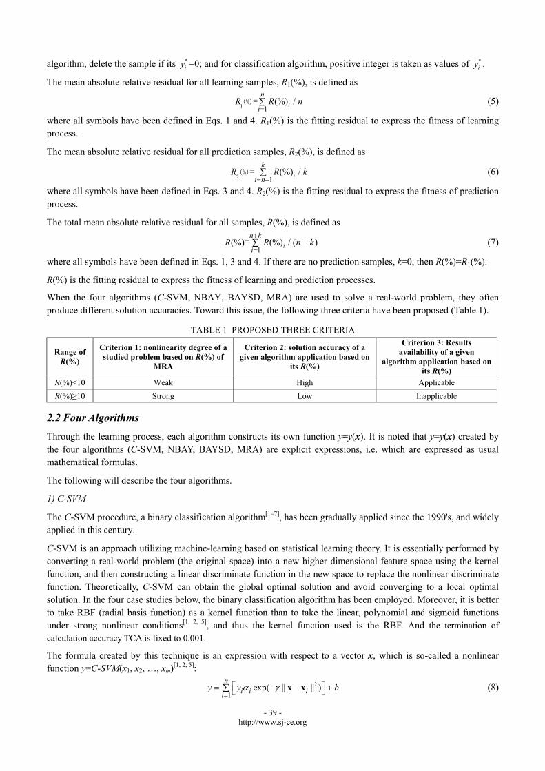
When the four algorithms (C-SVM, NBAY, BAYSD, MRA) are used to solve a real-world problem, they often produce different solution accuracies. Toward this issue, the following three criteria have been proposed (Table 1).

TABLE 1 PROPOSED THREE CRITERIA

Range of R(%)

Criterion 1: nonlinearity degree of a studied problem based on R(%) of

MRA

Criterion 2: solution accuracy of a given algorithm application based on

its R(%)

Criterion 3: Results availability of a given

algorithm application based on its R(%)

R(%)<10 Weak High Applicable

R(%)≥10 Strong Low Inapplicable

2.2 Four Algorithms

Through the learning process, each algorithm constructs its own function y=y(x). It is noted that y=y(x) created by the four algorithms (C-SVM, NBAY, BAYSD, MRA) are explicit expressions, i.e. which are expressed as usual mathematical formulas.

The following will describe the four algorithms.

1) C-SVM

The C-SVM procedure, a binary classification algorithm[1–7], has been gradually applied since the 1990's, and widely applied in this century.

C-SVM is an approach utilizing machine-learning based on statistical learning theory. It is essentially performed by converting a real-world problem (the original space) into a new higher dimensional feature space using the kernel function, and then constructing a linear discriminate function in the new space to replace the nonlinear discriminate function. Theoretically, C-SVM can obtain the global optimal solution and avoid converging to a local optimal solution. In the four case studies below, the binary classification algorithm has been employed. Moreover, it is better to take RBF (radial basis function) as a kernel function than to take the linear, polynomial and sigmoid functions under strong nonlinear conditions[1, 2, 5], and thus the kernel function used is the RBF. And the termination of

calculation accuracy TCA is fixed to 0.001.

The formula created by this technique is an expression with respect to a vector x, which is so-called a nonlinear function y=C-SVM(x1, x2, …, xm)[1, 2, 5]:

2

1exp( || || )

n

i i ii

y y b

x x (8)


where α is the vector of Lagrange multipliers, α=(α1, α2, …, αn), 0≤αi≤C where C is the penalty factor, and the

constraint 1

n

i ii

y =0; 2exp( || || )i x x is a RBF kernel function; γ is the regularization parameter, γ>0; and b is the

offset of the separating hyperplane, which can be calculated using the free vectors xi. These free xi are those vectors corresponding to αi>0, on which the final C-SVM model depends.

αi, C, and γ can be solved using the dual quadratic optimization:

2

1 , 1

1max exp( || || )

2

n n

i i j i j i ji i j

y y

α

x x (9)

It is noted that in the four case studies below the formulas corresponding to Eq. 8 are not concretely written out due to their large size.

2) NBAY

The NBAY procedure has been widely applied since the 1990's, and widely applied in this century[1, 2, 8]. The following introduces a NBAY technique, i.e. the naïve Bayesian. The formula created by this technique is a set of nonlinear products with respect to m parameters (x1, x2, …, xm)[1, 2, 9, 10]:

2

21

( )1

22( ) exp j jl

jljl

mjl

xN

x (l=1, 2, …, L) (10)

where l is the class number, L is the number of classes, Nl(x) is the discrimination function of the lth class with respect to x, σjl is the mean square error of xj in Class l, μjl is the mean of xj in Class l. Eq. 10 is so-called a naïve Bayesian discrimination function.

Once Eq. 10 is created, any sample shown by Eq. 1 or Eq. 3 can be substituted in Eq. 10 to obtain L values: N1, N2, …, NL. If

b 1max ll l L

N N

, then

y=lb (11) for this sample.

Eq. 11 is so-called a nonlinear function y=NBAY (x1, x2, …, xm).

3) BAYSD

The BAYSD procedure has been widely applied since the 1990's, and widely applied in this century[1, 2, 11, 12]. The following introduces BAYSD technique. The formula created by this technique is a set of nonlinear combinations with respect to m parameters (x1, x2,…, xm), plus two constant terms[1, 2]:

0 1( ) ln( ) ( 1,2,... )

m

jl l l jljB p c c x l L

x (12)

where l is the class number, L is the number of classes, Bl(x) is the discrimination function of the lth class with respect to x, cjl is the coefficient of xj in the lth discrimination function, pl and c0l are two constant terms in the lth discrimination function. The constants pl, c0l, c1l, c2l, …, cml are deduced using Bayesian theorem and calculated by the successive Bayesian discrimination of BAYSD. Eq. 12 is so-called a Bayesian discrimination function. In rare cases an introduced xk can be deleted in the Bayesian discrimination function, and in much rarer cases a deleted xk

could be again introduced into the Bayesian discrimination function. Therefore, usually Eq. 12 is solved via m iterations.

Once Eq. 12 is created, any sample shown by Eq. 1 or Eq. 3 can be substituted in Eq. 12 to obtain L values: B1, B2, …, BL. If

b 1max ll l L

B B

, then

y=lb (13) for this sample.

Eq. 13 is so-called a nonlinear function y=BAYSD(x1, x2, …, xm).

4) MRA

The MRA procedure has been widely applied since the 1970's, and the successive regression analysis, the most


popular MRA technique, is still a very useful tool[1, 2, 13, 14]. The formula created by this technique is a linear combination with respect to m parameters (x1, x2, …, xm), plus a constant term, which is so-called a linear function y=MRA(x1, x2, …, xm)[1, 2]:

y=b0+b1x1+b2x2+…+bmxm (14) where the constants b0, b1, b2, …, bm are deduced using regression criteria and calculated by the successive regression analysis of MRA. Eq. 14 is a so-called “regression equation”. In rare cases an introduced xk can be deleted in the regression equation, and in much rarer cases a deleted xk could be again introduced into the regression equation. Therefore, usually Eq. 14 is solved via m iterations.

2.3 Dimensionality Reduction

The definition of dimensionality reduction is to reduce the number of dimensions of a data space as small as possible but the results of studied problem are unchanged. The benefits of dimensionality reduction are to reduce the amount of data can enhance the calculating speed, to reduce the independent variables can extend applying ranges, and to reduce misclassification ratio of prediction samples can enhance processing quality.

Among the aforementioned four algorithms, each of MRA and BAYSD can serve as a promising dimension-reduction tool, respectively, because the two algorithms all can give the dependence of the predicted value (y) on independent variables (x1, x2, …, xm), in decreasing order. However, because MRA belongs to data analysis in linear correlation whereas BAYSD is in nonlinear correlation, in applications the preferable tool is BAYSD, whereas MRA is applicable only when the studied problems are linear. The called “promising tool” means whether it succeeds or not that needs a high-class nonlinear tool (e.g., C-SVM) for the validation, so as to determine how many independent variables can be reduced. For instance, Case study 1 below can be reduced from 5-D problem (x1, x2, x3, x4, y) to 2-D problem (x3, y) by using BAYSD and C-SVM; Case study 3 below cannot be reduced from 9-D problem (x1, x2, x3, x4, x5, x6, x7, x8, y) to 8-D problem (x2, x3, x4, x5, x6, x7, x8, y) by using BAYSD and C-SVM.

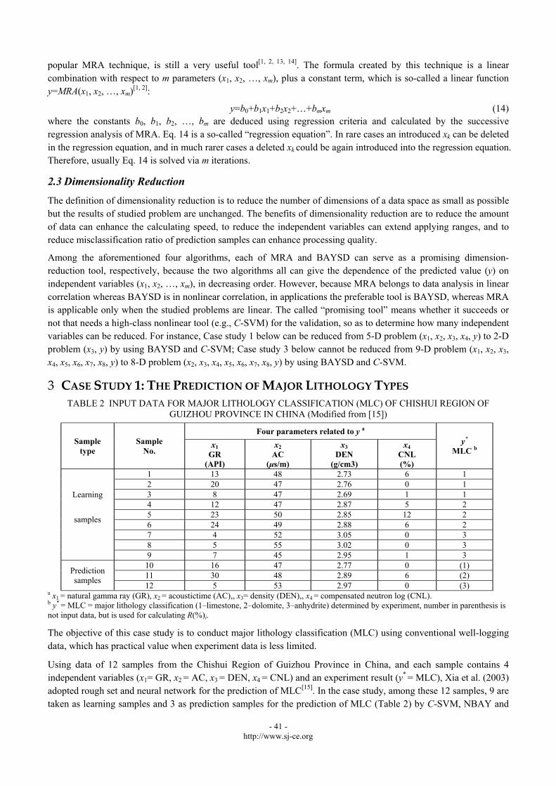
3 CASE STUDY 1: THE PREDICTION OF MAJOR LITHOLOGY TYPES

TABLE 2 INPUT DATA FOR MAJOR LITHOLOGY CLASSIFICATION (MLC) OF CHISHUI REGION OF GUIZHOU PROVINCE IN CHINA (Modified from [15])

Sample type

Sample No.

Four parameters related to y a y*

MLC b x1

GR (API)

x2

AC (μs/m)

x3

DEN (g/cm3)

x4

CNL (%)

Learning

samples

1 13 48 2.73 6 1 2 20 47 2.76 0 1 3 8 47 2.69 1 1 4 12 47 2.87 5 2 5 23 50 2.85 12 2 6 24 49 2.88 6 2 7 4 52 3.05 0 3 8 5 55 3.02 0 3 9 7 45 2.95 1 3

Prediction samples

10 16 47 2.77 0 (1) 11 30 48 2.89 6 (2) 12 5 53 2.97 0 (3)

a x1 = natural gamma ray (GR), x2 = acoustictime (AC),, x3= density (DEN),, x4 = compensated neutron log (CNL). b y* = MLC = major lithology classification (1–limestone, 2–dolomite, 3–anhydrite) determined by experiment, number in parenthesis is not input data, but is used for calculating R(%)i.

The objective of this case study is to conduct major lithology classification (MLC) using conventional well-logging data, which has practical value when experiment data is less limited.

Using data of 12 samples from the Chishui Region of Guizhou Province in China, and each sample contains 4 independent variables (x1= GR, x2 = AC, x3 = DEN, x4 = CNL) and an experiment result (y*

= MLC), Xia et al. (2003) adopted rough set and neural network for the prediction of MLC[15]. In the case study, among these 12 samples, 9 are taken as learning samples and 3 as prediction samples for the prediction of MLC (Table 2) by C-SVM, NBAY and


BAYSD.

3.1 Learning Process

Using the 9 learning samples (Table 2) and by C-SVM, NBAY, BAYSD and MRA, the following four functions of MLC (y) with respect to 4 independent variables (x1, x2, x3, x4) have been constructed.

Using C-SVM, the result is an explicit nonlinear function corresponding to Eq. 8:

y=C-SVM(x1, x2, x3, x4) (15) with C=32768, =0.000031, 7 free vectors xi, and the cross validation accuracy CVA=88.9%.

Using NBAY, the result is an explicit nonlinear discriminate function corresponding to Eq. 10:

2

2

41

( )1

22( ) exp j jl

jljl

jl

xN

x (l=1, 2, 3) (16)

where for l=1, σj1=4.92, 0.471, 0.029, 2.63, μj1=13.7, 47.3, 2.73, 2.33; for l=2, σj2=5.44, 1.25, 0.012, 3.09, μj2=19.7, 48.7, 2.87, 7.67; for l=3, σj3=1.25, 4.19, 0.042, 0.471, μj3=5.33, 50.7, 3.01, 0.333.

Using BAYSD, the result is an explicit nonlinear discriminate function corresponding to Eq. 12:

1 1 2 3 4

2 1 2 3 4

3 1 2 3 4

ln(0.333) 4733 6.75 25.5 3929 20.7ln(0.333) 5339 7.05 27.3 4177 22.6ln(0.333) 5821 7.83 28.4 6362 22.9

B x x x xB x x x xB x x x x

xxx

(17)

From the successive process, MLC (y) is shown to depend on the 4 independent variables in decreasing order: x3, x4, x2, and x1.

Though MRA is a regression algorithm rather than a classification algorithm, MRA can provide the nonlinearity degree of the studied problem, and thus it is required to run MRA.

Using MRA, the result is an explicit linear function corresponding to Eq. 14:

y=−!5.9−0.0196x1−0.0475x2+7.11x3+0.0317x4 (18) Equation 18 yields a residual variance of 0.0337 and a multiple correlation coefficient of 0.983. From the regression process, MLC (y) is shown to depend on the 4 independent variables in decreasing order: x3, x2, x1, and x4.

3.2 Prediction Process

Substituting the values of 4 independent variables (x1, x2, x3, x4) given by the 9 learning samples and 3 prediction samples (Table 2) in Eqs. 15, 16 (and then use Eq. 11), 17 (and then use Eq. 13) and 18, respectively, the MLC (y) of each sample is obtained (Table 3).

TABLE 3 PREDICTION RESULTS FROM MAJOR LITHOLOGY CLASSIFICATION (MLC) OF CHISHUI REGION OF GUIZHOU PROVINCE IN CHINA

Sample type

Sample No.

MLC a

y* Classification algorithm

MRA C-SVM NBAY BAYSD

y R(%) y R(%) y R(%) y R(%)

Learning samples

1 1 1 0 1 0 1 0 1.15 14.9 2 1 1 0 1 0 1 0 1.08 8.30 3 1 1 0 1 0 1 0 0.852 14.8 4 2 2 0 2 0 2 0 2.18 9.00 5 2 2 0 2 0 2 0 1.90 4.91 6 2 2 0 2 0 2 0 1.95 2.35 7 3 3 0 3 0 3 0 3.22 7.36 8 3 3 0 3 0 3 0 2.85 5.15 9 3 3 0 3 0 3 0 2.82 6.17

Prediction samples

10 1 1 0 1 0 1 0 1.23 23.2 11 2 2 0 2 0 2 0 1.95 2.29 12 3 3 0 3 0 3 0 2.59 13.8

a y* = MLC = major lithology classification (1–limestone, 2–dolomite, 3–anhydrite) determined by experiment.


TABLE 4 COMPARISON AMONG THE APPLICATIONS OF CLASSIFICATION ALGORITHMS (C-SVM, NBAY AND BAYSD) TO MAJOR LITHOLOGY CLASSIFICATION (MLC) OF CHISHUI REGION OF GUIZHOU

PROVINCE IN CHINA

Algorithm Fitting

formula

Mean absolute relative residual

Dependence of the predicted value (y) on independent

variables (x1, x2, x3, x4), in

decreasing order

Time consuming

on PC (Intel

Core 2)

Problem nonlinearity

Solution accuracy

Results availability

R1(%) R2(%) R(%)

C-SVM Nonlinear,

explicit 0 0 0 N/A 5 s N/A High Applicable

NBAY Nonlinear,

explicit 0 0 0 N/A <1 s N/A High Applicable

BAYSD Nonlinear,

explicit 0 0 0 x3, x4, x2, x1 1 s N/A High Applicable

MRA Linear, explicit

8.11 13.1 9.36 x3, x2, x1, x4 <1 s Weak N/A N/A

From Table 4 and based on Table 1, it shown that a) the nonlinearity degree of this studied problem is weak since R(%) of MRA is 9.36; b) the solution accuracies of C-SVM, NBAY and BAYSD are high due to the fact that their R(%) values are all 0; and c) the results availability of C-SVM, NBAY and BAYSD are applicable due to the indication that their R(%) values are all 0.

3.3 Dimension-reduction succeeded from 5-D to 2-D problem by using BAYSD and C-SVM

BAYSD gives the dependence of the predicted value (y) on 4 independent variables, in decreasing order: x3, x4, x2, x1 (Table 4). According to this dependence order, at first, deleting x1 and running C-SVM, it is found the results of C-SVM are the same as before, i.e., R(%)=0, thus 5-D problem (x1, x2, x3, x4, y) can become 4-D problem (x2, x3, x4, y). In the same way, it is found that this 4-D problem can become 3-D problem by deleting x2, this 3-D problem can become 2-D problem by deleting x4. Therefore, the 5-D problem (x1, x2, x3, x4, y) at last can become 2-D problem (x3, y).

4 CASE STUDY 2: THE PREDICTION OF OIL LAYER

The objective of this case study is to conduct oil layer classification in clayey sandstone using conventional well-logging data, which has practical value when oil test data is less limited.

From Table 5 and based on Table 1, it shown that a) the nonlinearity degree of this studied problem is weak since R(%) of MRA is 5.04; b) the solution accuracies of C-SVM, NBAY and BAYSD are high due to the fact that their R(%) values are all 0; and c) the results availability of C-SVM, NBAY and BAYSD are applicable due to the indication that their R(%) values are all 0.

TABLE 5 COMPARISON AMONG THE APPLICATIONS OF CLASSIFICATION ALGORITHMS (C-SVM, NBAY AND BAYSD) TO OIL LAYER CLASSIFICATION OF LOWER H3 FORMATION IN XIA’ERMEN OILFIELD OF

HENAN OIL PROVINCE IN CENTRAL CHINA (Modified from [2])

Algorithm Fitting

formula


Dependence of the predicted value (y) on independent variables (x1, x2, …, x8), in

decreasing order

Time consuming

on PC (Intel

Core 2)


Solution accuracy


R1(%) R2(%) R(%)

C-SVM Nonlinear,


NBAY Nonlinear,

explicit 0 0 0 N/A <1 s N/A High Applicable

BAYSD Nonlinear,

explicit 0 0 0

x5, x8 x6, x1, x3, x2, x4, x7

1 s N/A High Applicable


1.68 15.11 5.04x5, x8 x6, x1, x4, x2,

x3, x7 <1 s Weak N/A N/A


TABLE 6 INPUT DATA FOR HYDROCARBON LAYER CLASSIFICATION (HLC) OF TARIM BASIN IN WESTERN CHINA (Modified from [16])

Sample type

Sample No.

Well No.

Interval (m)

Eight parameters related to y a y*

HLCx1

H (m)

x2

RT (Ω·m)

x3

RXO (Ω·m)

x4

SP (mv)

x5

GR (API)

x6

AC (μs/m)

x7

CNL (%)

x8

DEN (g/cm3)

Learning samples

1 Lu9 1031.3–1034 2.7 8 8.6 -56.9 58.9 108 27 2.11 1

2 Lu9 1037–1042 5.1 5 6.1 -57.6 60 105 35 2.15 4

3 Lu9 1122.5–1127 4.6 5 7 -53.7 55 106 32.9 2.17 4

4 Lu9 1186–1192 6.1 9 9.4 -54.4 61.6 104.2 31.8 2.16 3

5 Lu9 1233–1237 4.1 7 8.3 -59.1 64 106 34.3 2.13 3

6 Lu9 1295-1299.1 4.1 5 7.2 -58.4 64.9 102 32.4 2.16 4

7 Lu9 1323.1–1328 5 7 9 -58 67.4 104 33.1 2.14 2

8 Lu9 1415–1418 3.1 11 8.3 -58 63.9 99.9 33.1 2.15 2

9 Lu9 1424–1426 2.1 5 8.3 -58.2 67.4 102 32.3 2.14 2

10 Lu9 1434–1437 2.8 5 7.5 -60.1 67.4 102 32.3 2.14 4

11 Lu101 1180–1187.7 6.8 6 5.2 -20.2 62 106 32.2 2.12 3

12 Lu101 1273–1275 2.1 7 11 -22.6 65 94.9 30.4 2.22 3

13 Lu101 1409–1413 4.8 7 5.9 -24.5 68 98 30.9 2.18 2

14 Lu102 1216–1219 3.1 5 4.6 -5.4 64.6 102 34.1 2.16 3

15 Lu102 1400–1403.3 3.3 5 5.4 -7.8 69.3 105 32.7 2.14 3

16 Lu103 1367–1270 3.1 9 11 -11.2 65.4 103 33.9 2.13 3

17 Lu103 1352–1356 4.1 13 15 -16 70.5 96.9 30.9 2.2 3

18 Lu104 1002–1010 8 5 14 -20.9 65.8 105 33.4 2.16 4

19 Lu104 1192.2–1194 1.9 5 14 -20.9 65.8 105 33.4 2.16 4

20 Lu104 1202–1208 6.6 6 6 -17.9 82.1 98 32.1 2.3 3

21 Lu104 1214–1218.9 5 5 5 -20.3 60.9 104 33.7 2.13 4

22 Lu108 1030–1036 6.1 5 6.7 -49.5 64 107 35.3 2.15 4

23 Lu108 1122–1126 4.1 5 7 -49.8 69.2 108 34.4 2.16 4

24 Lu108 1215–1217 2.1 6 7.9 -52.4 77.2 103 34.8 2.17 4

25 Lu109 1346–1350 3.4 8 8.6 -25.6 65 97.5 31.9 2.18 3

26 Lu111 1166.8–1172 5.2 11 13 -74.4 61.1 111 31.4 2.14 2

27 Lu111 1197–1202 5.1 8 9.7 -72.4 64.1 120 30.7 2.12 3

28 Lu111 1276–1278 1.9 7 9.3 -71.1 64.2 111 31.1 2.12 3

29 Lu112 1133–1136 3.1 6 6.2 -14.8 77.4 102 32.3 2.2 4

30 Lu112 1225–1228 2.1 5 6.2 -18.7 69.5 104 33.5 2.14 4

31 Lu113 1264.5–1266 1.5 6 6.8 -30.5 74.1 99.2 31.4 2.23 4

32 Lu113 1334–1335 1.1 7 7.2 -43.1 67.2 102 33.4 2.19 2

33 Lu113 1333.8–1340 2.1 6 7.3 -48.2 64.6 97.9 30.6 2.19 4

Prediction samples

34 Lu102 1164–1168 4.1 7 4.9 -5.2 64.2 106 33 2.12 (3)

a x1= thickness (H), x2 = true formation resistivity (RT), x3 = micro-spherically focused log (RXO), x4 = spontaneous potential (SP), x5 = natural gamma ray (GR), x6 = acoustictime (AC), x7 = compensated neutron log (CNL), x8= density (DEN). b y* = HLC = hydrocarbon layer classification (1–gas layer, 2–oil layer, 3–water/oil layer, 4–water layer) determined by the well test, number in parenthesis is not input data, but is used for calculating R(%)i.

5 CASE STUDY 3: THE PREDICTION OF HYDROCARBON LAYER

The objective of this case study is to conduct hydrocarbon layer classification (HLC) using conventional well-logging data, which has practical value when well test data is less limited.

Using data of 34 samples from the Tarim Basin in western CHINA, and each sample contains 8 independent variables (x1= H, x2 = RT, x3 = RXO, x4 = SP, x5 = GR, x6 = AC, x7 = CNL, x8 = DEN) and a well test result (y*

= HLC), Wang et al. (2007) adopted fuzzy clustering for the prediction of HLC[16]. In the case study, among these 34 samples, 33 are taken as learning samples and one as prediction sample for the prediction of HLC (Table 6) by C-SVM, NBAY and BAYSD.


5.1 Learning Process

Using the 33 learning samples (Table 6) and by C-SVM, NBAY, BAYSD and MRA, the following four functions of HLC (y) with respect to 8 independent variables (x1, x2, x3, x4, x5, x6, x7, x8) have been constructed.

Using C-SVM, the result is an explicit nonlinear function corresponding to Eq. 8:

y=C-SVM(x1, x2, x3, x4, x5, x6, x7, x8) (19)

with C=8, =2, 33 free vectors xi, and the cross validation accuracy CVA=54.5%.

Using NBAY, the result is an explicit nonlinear discriminate function corresponding to Eq. 10:

2

2

81

( )1

22( ) exp j jl

jljl

jl

xN

x (l=1, 2, 3, 4) (20)

where for l=1, σj1=0, 0, 0, 0, 0, 0, 0, 0, μj1=2.7, 8, 8.6, -56.9, 58.9, 108, 27, 2.11; for l=2, σj2=1.57, 2.24, 2.2, 15.5, 2.5, 4.11, 0.934, 0.021, μj2=3.55, 8, 8.62, -52.7, 65.8, 103, 32.4, 2.16; for l=3, σj3=1.59, 2.1, 2.88, 23.9, 5.31, 6.64, 1.29, 0.052, μj3=4.14, 7.5, 8.63, -32, 66.5, 104, 32.2, 2.17; for l=4, σj4=1.81, 0.452, 2.63, 16.8, 6.13, 2.71, 1.32, 0.026, μj4=3.76, 5.29, 7.78, -39.7, 66.8, 104, 33.2, 2.17.

Using BAYSD, the result is an explicit nonlinear discriminate function corresponding to Eq. 12:

1 1 2 3 4 5 6 7 8

2 1 2 3 4 5 6 7 8

3 1 2 3 4

ln(0.030) 7066 25.7 11.7 1.225 1.43 13.5 28.1 47.2 5064

ln(0.182) 7315 25.6 11.8 0.833 1.34 13.4 27.8 51.5 5128

ln(0.364) 7372 25.6 11.8 0.826 1.43 13

B x x x x x x x x

B x x x x x x x x

B x x x x

x

x

x

5 6 7 8

4 1 2 3 4 5 6 7 8

.5 28.1 51.2 5148

ln(0.424) 7393 25.6 10.7 0.503 1.37 13.4 28.0 51.9 5156

x x x x

B x x x x x x x x

x

(21)

From the successive process, HLC (y) is shown to depend on the 8 independent variables in decreasing order: x7, x2, x8, x4, x6, x3, x5, and x1.

Though MRA is a regression algorithm rather than a classification algorithm, MRA can provide the nonlinearity degree of the studied problem, and thus it is required to run MRA.

Using MRA, the result is an explicit linear function corresponding to Eq. 14:

y=−18.1−0.012x1−0.215x2+0.074x3+0.00311x4 −0.0106x5+0.0223x6+0.184x7+6.81x8 (22)

Equation 22 yields a residual variance of 0.52 and a multiple correlation coefficient of 0.693. From the regression process, HLC (y) is shown to depend on the 8 independent variables in decreasing order: x2, x7, x3, x8, x6, x4, x5, and x1.

5.2 Prediction Process

Substituting the values of 8 independent variables (x1, x2, x3, x4, x5, x6, x7, x8) given by the 33 learning samples and 1 prediction sample (Table 6) in Eqs. 19, 20 (and then use Eq. 11), 21 (and then use Eq. 13) and 22, respectively, the HLC (y) of each sample is obtained (Table 7).

From Table 8 and based on Table 1, it shown that a) the nonlinearity degree of this studied problem is strong since R(%) of MRA is 18.3; b) the solution accuracies of C-SVM, NBAY and BAYSD are high, low and low due to the fact that their R(%) are 0, 19.4 and 12.3, respectively; and c) the results availability of C-SVM, NBAY and BAYSD are applicable, inapplicable and inapplicable due to the indication that their R(%) are 0, 19.4 and 12.3, respectively.

5.3 Dimension-reduction Failed by Using BAYSD and C-SVM

BAYSD gives the dependence of the predicted value (y) on 8 independent variables, in decreasing order: x7, x2, x8, x4, x6, x3, x5, x1 (Table 8). According to this dependence order, at first, deleting x1 and running C-SVM, it is found the results of C-SVM are changed with R(%)=3.68 which is greater than previous R(%)=0 (Table 8). Thus the 9-D problem (x1, x2, x3, x4, x5, x6, x7, x8, y) cannot become 8-D problem (x2, x3, x4, x5, x6, x7, x8, y), showing that the expression of y needs all of x1, x2, x3, x4, x5, x6, x7, x8. In general, the dimension-reduction succeeds for high-dimensional problem[1, 4, 7].


TABLE 7 PREDICTION RESULTS FROM HYDROCARBON LAYER CLASSIFICATION (HLC) OF TARIM BASIN IN WESTERN CHINA

Sample type

Sample No.

HLC a

y* Classification algorithm

MRA C-SVM NBAY BAYSD

y R(%) y R(%) y R(%) y R(%)

Learning samples

1 1 1 0 3 200 1 0 1.69 68.9 2 4 4 0 4 0 4 0 3.79 5.36 3 4 4 0 4 0 4 0 3.69 7.64 4 3 3 0 2 33.3 3 0 2.61 13.0 5 3 3 0 2 33.3 4 33.3 3.24 8.01 6 4 4 0 4 0 4 0 3.35 16.3 7 2 2 0 2 0 2 0 3.05 52.6 8 2 2 0 2 0 2 0 2.18 8.80 9 2 2 0 2 0 4 100 3.27 63.6

10 4 4 0 2 50 4 0 3.20 20.0 11 3 3 0 4 33.3 3 0 2.88 3.97 12 3 3 0 3 0 3 0 3.21 7.14 13 2 2 0 3 50 3 50 2.66 32.8 14 3 3 0 4 33.3 3 0 3.65 21.6 15 3 3 0 4 33.3 3 0 3.32 10.7 16 3 3 0 3 0 3 0 3.02 0.520 17 3 3 0 3 0 3 0 2.16 28.0 18 4 4 0 4 0 4 0 4.16 4.03 19 4 4 0 4 0 4 0 4.23 5.86 20 3 3 0 3 0 4 33.3 3.77 25.6 21 4 4 0 4 0 3 25 3.41 14.7 22 4 4 0 4 0 4 0 3.90 2.49 23 4 4 0 4 0 4 0 3.82 4.61 24 4 4 0 4 0 4 0 3.63 9.28 25 3 3 0 2 33.3 3 0 2.86 4.71 26 2 2 0 3 50 3 50 2.34 17.2 27 3 3 0 3 0 3 0 2.66 11.5 28 3 3 0 2 33.3 3 0 2.76 8.16 29 4 4 0 4 0 3 25 3.33 16.8 30 4 4 0 4 0 4 0 3.48 12.9 31 4 4 0 3 25 4 0 3.35 16.2 32 2 2 0 2 0 4 100 3.36 68.2 33 4 4 0 2 50 4 0 2.98 25.5

Prediction samples

10 3 3 0 3 0 3 0 2.85 5.11

a y* = HLC = hydrocarbon layer classification (1–gas layer, 2–oil layer, 3–water/oil layer, 4–water layer) determined by the well test.

TABLE 8 COMPARISON AMONG THE APPLICATIONS OF CLASSIFICATION ALGORITHMS (C-SVM, NBAY AND BAYSD) TO HYDROCARBON LAYER CLASSIFICATION (HLC) OF TARIM BASIN IN WESTERN CHINA

Algorithm Fitting

formula



decreasing order

Time consuming

on PC (Intel Core

2)


Solution accuracy


R1(%) R2(%) R(%)

C-SVM Nonlinear,


NBAY Nonlinear,

explicit 20.0 0 19.4 N/A <1 s N/A Low Inapplicable

BAYSD Nonlinear,

explicit 12.6 0 12.3

x7, x2, x8, x4, x6, x3, x5, x1

1 s N/A Low Inapplicable


18.7 5.11 18.3 x2, x7, x3, x8, x6, x4,

x5, x1 <1 s Strong N/A N/A

6 CASE STUDY 4: THE PREDICTION OF FRACTURE

The objective of this case study is to predict fractures using conventional well-logging data, which has practical


values when the data of imaging log and core sample are limited.

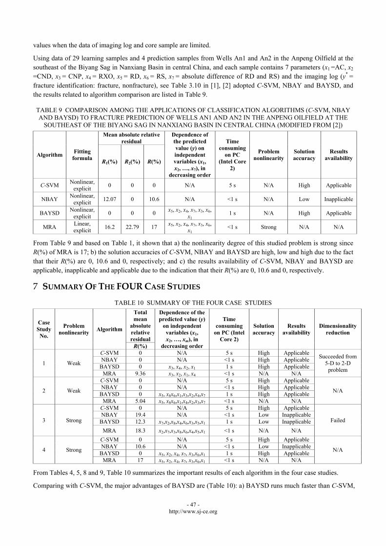
Using data of 29 learning samples and 4 prediction samples from Wells An1 and An2 in the Anpeng Oilfield at the southeast of the Biyang Sag in Nanxiang Basin in central China, and each sample contains 7 parameters (x1 =AC, x2

=CND, x3 = CNP, x4 = RXO, x5 = RD, x6 = RS, x7 = absolute difference of RD and RS) and the imaging log (y* =

fracture identification: fracture, nonfracture), see Table 3.10 in [1], [2] adopted C-SVM, NBAY and BAYSD, and the results related to algorithm comparison are listed in Table 9.

TABLE 9 COMPARISON AMONG THE APPLICATIONS OF CLASSIFICATION ALGORITHMS (C-SVM, NBAY AND BAYSD) TO FRACTURE PREDICTION OF WELLS AN1 AND AN2 IN THE ANPENG OILFIELD AT THE

SOUTHEAST OF THE BIYANG SAG IN NANXIANG BASIN IN CENTRAL CHINA (MODIFIED FROM [2])

Algorithm Fitting

formula



decreasing order

Time consuming

on PC (Intel Core

2)


Solution accuracy


R1(%) R2(%) R(%)

C-SVM Nonlinear,


NBAY Nonlinear,

explicit 12.07 0 10.6 N/A <1 s N/A Low Inapplicable

BAYSD Nonlinear,

explicit 0 0 0

x5, x2, x4, x7, x3, x6, x1

1 s N/A High Applicable


16.2 22.79 17 x5, x2, x4, x7, x3, x6,

x1 <1 s Strong N/A N/A

From Table 9 and based on Table 1, it shown that a) the nonlinearity degree of this studied problem is strong since R(%) of MRA is 17; b) the solution accuracies of C-SVM, NBAY and BAYSD are high, low and high due to the fact that their R(%) are 0, 10.6 and 0, respectively; and c) the results availability of C-SVM, NBAY and BAYSD are applicable, inapplicable and applicable due to the indication that their R(%) are 0, 10.6 and 0, respectively.

7 SUMMARY OF THE FOUR CASE STUDIES

TABLE 10 SUMMARY OF THE FOUR CASE STUDIES

Case Study

No.


Algorithm

Total mean

absolute relative residual

Dependence of the predicted value (y)

on independent variables (x1, x2, …, xm), in

decreasing order

Time consuming

on PC (Intel Core 2)

Solution accuracy


Dimensionalityreduction

R(%)

1 Weak

C-SVM 0 N/A 5 s High Applicable Succeeded from

5-D to 2-D problem

NBAY 0 N/A <1 s High Applicable BAYSD 0 x3, x4, x2, x1 1 s High Applicable

MRA 9.36 x3, x2, x1, x4 <1 s N/A N/A

2 Weak

C-SVM 0 N/A 5 s High Applicable

N/A NBAY 0 N/A <1 s High Applicable

BAYSD 0 x5, x8x6,x1,x3,x2,x4,x7 1 s High Applicable MRA 5.04 x5, x8x6,x1,x4,x2,x3,x7 <1 s N/A N/A

3 Strong


Failed NBAY 19.4 N/A <1 s Low Inapplicable

BAYSD 12.3 x7,x2,x8,x4,x6,x3,x5,x1 1 s Low Inapplicable

MRA 18.3 x2,x7,x3,x8,x6,x4,x5,x1 <1 s N/A N/A

4 Strong


N/A NBAY 10.6 N/A <1 s Low Inapplicable

BAYSD 0 x5, x2, x4, x7, x3,x6,x1 1 s High Applicable MRA 17 x5, x2, x4, x7, x3,x6,x1 <1 s N/A N/A

From Tables 4, 5, 8 and 9, Table 10 summarizes the important results of each algorithm in the four case studies.

Comparing with C-SVM, the major advantages of BAYSD are (Table 10): a) BAYSD runs much faster than C-SVM,


b) it is easy to code the BAYSD program whereas very complicated to code the C-SVM program, and c) BAYSD can serve as a promising dimension-reduction tool. So BAYSD is better than C-SVM when nonlinearity of studied problem is weak.

8 CONCLUSIONS

Through the aforementioned four case studies, five major conclusions can be drawn as follows:

1) the total mean absolute relative residual R(%) of MRA can be used to measure the nonlinearity degree of a studied problem, and thus MRA should be run at first;

2) the proposed three criteria [nonlinearity degree of a studied problem based on R(%) of MRA, solution accuracy of a given algorithm application based on its R(%), results availability of a given algorithm application based on its R(%)] are practical;

3) if a classification problem has weak nonlinearity, in genaral, C-SVM, NBAY and BAYSD are applicable, and BAYSD is better than C-SVM and NBAY;

4) any of NBAY cannot be applied to any classification problems with strong nonlinearity, but BAYSD sometims could be applied, and C-SVM always could be applied;

5) BAYSD and C-SVM can be applied to dimensionality reduction.

ACKNOWLEDGMENT

This work was supported by the Research Institute of Petroleum Exploration and Development (RIPED) and PetroChina.

REFERENCES

[1] Shi G. “Data Mining and Knowledge Discovery for Geoscientists.” Elsevier Inc, USA, 2013

[2] Shi G. “Optimal prediction in petroleum geology by regression and classification methods.” Sci J Inf Eng 5(2): 14-32, 2015

[3] Shi G. “The use of support vector machine for oil and gas identification in low-porosity and low-permeability reservoirs.” Int J

Math Model Numer Optimisa 1(1/2): 75-87, 2009

[4] Shi G, Yang X. “Optimization and data mining for fracture prediction in geosciences.” Procedia Comput Sci 1(1): 1353-1360, 2010

[5] Chang C, Lin C. “LIBSVM: a library for support vector machines, Version 3.1.” Retrieved from www.csie.ntu.edu.tw/~cjlin

/libsvm, 2011

[6] Zhu Y, Shi G. “Identification of lithologic characteristics of volcanic rocks by support vector machine.” Acta Petrolei Sinica 34(2):

312-322, 2013

[7] Shi G, Zhu Y, Mi S, Ma J, Wan J. “A big data mining in petroleum exploration and development.” Adv Petrol Expl Devel 7(2): 1-

8, 2014

[8] Ramoni M, Sebastiani P. “Robust Bayes classifiers.” Artificial Intelligence 125(1-2): 207-224, 2001

[9] Tan P, Steinbach M, Kumar V. “Introduction to Data Mining.” Pearson Education, Boston, MA, USA, 2005

[10] Han J, Kamber M. “Data Mining: Concepts and Techniques, 2nd Ed.” Morgan Kaufmann, San Francisco, CA, USA, 2006

[11] Denison DGT, Holmes CC, Mallick BK, Smith AFM. “Bayesian Methods for Nonlinear Classification and Regression.” John

Wiley & Sons Inc, Chichester, England, UK, 2002

[12] Shi G. “Four classifiers used in data mining and knowledge discovery for petroleum exploration and development.” Adv Petrol

Expl Devel 2(2): 12-23, 2011

[13] Sharma MSR, O'Regan M, Baxter CDP, Moran K, Vaziri H, Narayanasamy R. “Empirical relationship between strength and

geophysical properties for weakly cemented formations.” J Petro Sci Eng 72(1-2): 134-142, 2010

[14] Singh J, Shaik B, Singh S, Agrawal VK, Khadikar PV, Deeb O, Supuran CT. “Comparative QSAR study on para-substituted

aromatic sulphonamides as CAII inhibitors: information versus topological (distance-based and connectivity) indices.” Chem Biol

Drug Design 71, 244-259, 2008

[15] Xia K, Song J, Li C. “An approach to oil log data mining based on rough set & neural network.” Information and Control 32(4):

300-303, 2003


[16] Wang Z, Wang X, Qu J, Fang H, Jian H. “Study and application of data mining technologe in petroleum exploration and

development.” Petrol Ind Comp Appl 15(1): 17-20, 2007

AUTHORS 1Guangren Shi was born in Shanghai,

China in February, 1940, Expert,

Professor with qualification of directing

Ph. D. students. He was graduated from

Xi’an Jiaotong University, China in 1963,

majoring in applied mathematics (1958–

1963). Since 1963, he has been engaged in

computer applications for petroleum

exploration and development. In the recent 30 years, his research

only contains two fields of basin modeling (petroleum system)

and data mining for geosciences. In the recent years, however,

he has focused on the latter more than the former.

He has more than 51 years of professional career, working for

the computer center, Daqing Oilfield, petroleum ministry, China,

as Associate Engineer and Head of software group (1963–1967);

for the computer center, Shengli Oilfield, petroleum ministry,

China, as Engineer and Director (1967–1978); for the computer

center, petroleum ministry, China, as Engineer and Head of

software group (1978–1985); for the Aldridge laboratory of

applied geophysics, Columbia university at New York City,

U.S.A, as Visiting Scholar (1985–1987); for the computer

application technology research department, Research Institute

of Petroleum Exploration and Development (RIPED), China

National Petroleum Corporation (CNPC), China, as Professor,

Director (1987–1997); for the RIPED, PetroChina Company

Limited (PetroChina), China, as Professor with qualification of

directing Ph. D. students, Deputy Chief Engineer (1997–2001);

and for the department of experts in RIPED of PetroChina,

China, as Expert, Professor with qualification of directing Ph. D.

students (2001–Present). He published eight books, in which

there are three in English, i.e. 1) Shi G. R. 2013. Data Mining

and Knowledge Discovery for Geoscientists. Elsevier Inc, USA.

367pp; 2) Shi G. R. 2005. Numerical Methods of Petroliferous

Basin Modeling, 3rd edition. Petroleum Industry Press, Beijing,

China. 338pp, which was book-reviewed by Mathematical

Geosciences in 2009; and 3) Shi G. R. 2000. Numerical Methods

of Petroliferous Basin Modeling, 2nd edition. Petroleum Industry

Press, Beijing, China. 233pp, which was book-reviewed by

Mathematical Geology in 2006. He also published 75 articles, in

which there are 17 in English, e.g. four articles indexed by SCI:

1) Shi G. R., Zhang Q., C., Yang X. S., Mi S. Y. 2010. Oil and

gas assessment of the Kuqa Depression of Tarim Basin in

western China by simple fluid flow models of primary and

secondary migrations of hydrocarbons. Journal of Petroleum

Science and Engineering, 75 (1-2): 77–90; 2) Shi G. R. 2009. A

simplified dissolution-precipitation model of the smectite to

illite transformation and its application. Journal of Geophysical

Research-Solid Earth, 114, B10205, doi:10.1029/2009JB006406;

3) Shi G. R. 2008. Basin modeling in the Kuqa Depression of

the Tarim Basin (Western China): A fully temperature-

dependent model of overpressure history. Mathematical

Geosciences, 40 (1): 47–62; and 4) Shi G. R., Zhou X. X.,

Zhang G. Y., Shi X. F., Li H. H. 2004. The use of artificial

neural network analysis and multiple regression for trap quality

evaluation: a case study of the Northern Kuqa Depression of

Tarim Basin in western China. Marine and Petroleum Geology,

21 (3): 411–420.

Prof. Shi is Member of Society of Petroleum Engineers

(International), Member of Chinese Association of Science and

Technology, Member of Petroleum Society of China. And he

also is Regional Editor (Asia), International Journal of

Mathematical Modelling and Numerical Optimisation, and

Member of Editorial Board, Journal of Petroleum Science

Research. He received three honors: 1) A Person Studying

Overseas and Return with Excellent Contribution, appointed by

the Ministry of Education of China (1991); 2) Special

Government Allowance, awarded by the State Council of China

(1994); and 3) Grand Award of Sun Yueqi Energy, awarded by

the Ministry of Science-Technology of China (1997). And he

also obtained four awards of Science-Technology Progress, in

which one is China National Award, and three are from CNPC

and PetroChina. 2Jinshan Ma, was born in Shandong

Province, China in November, 1974. He

was graduated from Shandong University,

China in 1998, majoring in computer

sciences (1994–1998), and received a

Bachelor of Science degree in computer

and application. From 1998 to 2000, he

was an assistant engineer at Shengli Oilfield, China, working for

China Petroleum and Chemical Corporation (Sinopec). He was

graduate student at the Research Institute of Petroleum

Exploration and Development (RIPED), Petrochina (2000–2003),

and received a Master of Engineering degree in mineral

prospecting and exploration. Since 2003, he has been working

for RIPED. His experiences with Shengli Oilfield and RIPED

are primarily in petroleum data management. He engages in

petroleum data managemeent and petroleum database design for

PetroChina. He participated directly in the effort of EPDM

(exploration and production data model) designing, which was


an oil and gas E&P data model for PetroChina and was released

in 2012 as enterprise standard. He participated in the publication

of several papers on petroleum data management, database

design, and data mining. He is now a Senior Engineer of

information management.

3Dan Ba, was born in Heilongjiang

Province, China in July, 1988. She was

graduated from Northeast Petroleum

University, China in 2011, majoring in

computer & information technology

(2007–2011), and received a Bachelor of

Engineering degree in computer science &

technology. Then she went aboard and studied at Queen Mary,

University of London, UK. At the end of 2012, received a

Master of Science degree in intelligent web technology, and

achieved a distinction honor. Particularly, her research fields are

primarily in information retrieval (semantic web) and data

interchange. In July 2013, she was employed by Research

Institute of Petroleum Exploration and Development, Petrochina,

China. Currently, she is an Assistant Engineer in establishing

global petroleum resources database system and developing oil

and gas resources evaluation software. She participated directly

in the design of data mining (dedicating on textual data mining)

tools, which is a sub-project belonging to one of the important

national science & technology specific project. Besides, she has

already participated in the publication of two papers, one on

Earth Science Frontiers while another one on China Petroleum

Exploration.

Documents

Optimal Selection of Classification Algorithms for Well Log Interpretation