Embed Size (px)
Citation preview

Optimal supply &Structure detection
Single Source
DistributedSourcesFacility location
Size-density law
A reasonable derivation
Global redistributionnetworks
StructureDetectionHierarchy by division
Hierarchy by shuffling
Spectral methods
Hierarchies & Missing Links
General structure detection
Final words
References
Frame 1/78
Optimal supply & Structure detectionComplex Networks, SFI Summer School, June, 2010
Prof. Peter Dodds
Department of Mathematics & StatisticsCenter for Complex Systems
Vermont Advanced Computing CenterUniversity of Vermont
Licensed under the Creative Commons Attribution-NonCommercial-ShareAlike 3.0 License.
Optimal supply &Structure detection
Single Source
DistributedSourcesFacility location
Size-density law
A reasonable derivation
Global redistributionnetworks
StructureDetectionHierarchy by division
Hierarchy by shuffling
Spectral methods
Hierarchies & Missing Links
General structure detection
Final words
References
Frame 2/78
Outline
Single Source
Distributed SourcesFacility locationSize-density lawA reasonable derivationGlobal redistribution networks
Structure DetectionHierarchy by divisionHierarchy by shufflingSpectral methodsHierarchies & Missing LinksGeneral structure detection
Final words
References
Optimal supply &Structure detection
Single Source
DistributedSourcesFacility location
Size-density law
A reasonable derivation
Global redistributionnetworks
StructureDetectionHierarchy by division
Hierarchy by shuffling
Spectral methods
Hierarchies & Missing Links
General structure detection
Final words
References
Frame 3/78
Optimal supply networks
What’s the best way to distribute stuff?
I Stuff = medical services, energy, nutrients, people, ...I Some fundamental network problems:
1. Distribut e stuff from single source to many sinks2. Collect stuff coming from many sources at a single
sink3. Distribute stuff from many sources to many sinks4. Redistribute stuff between many nodes
I Q: How do optimal solutions scale with system size?
Optimal supply &Structure detection
Single Source
DistributedSourcesFacility location
Size-density law
A reasonable derivation
Global redistributionnetworks
StructureDetectionHierarchy by division
Hierarchy by shuffling
Spectral methods
Hierarchies & Missing Links
General structure detection
Final words
References
Frame 4/78
Single source optimal supply
Basic Q for distribution/supply networks:
I How does flow behave given cost:
C =∑
j
I γj Zj
whereIj = current on link jandZj = link j ’s impedance?
I Example: γ = 2 for electrical networks.

Optimal supply &Structure detection
Single Source
DistributedSourcesFacility location
Size-density law
A reasonable derivation
Global redistributionnetworks
StructureDetectionHierarchy by division
Hierarchy by shuffling
Spectral methods
Hierarchies & Missing Links
General structure detection
Final words
References
Frame 5/78
Single source optimal supply
the potential at the nodes by solving the system of linearequations ik !
PlRkl"Uk #Ul$, then the currents through
the links Ikl are determined. We use these currents todetermine a first approximation of the optimal conductiv-ities on the basis of the scaling relation. Then, the currentsare recalculated with this set of conductivities, and thescaling relation is reused for the next approximation.These steps are repeated until the values have converged.We check by perturbing the solution that it actually is aminimum of the dissipation, which was always the case.
For all !> 1, independently of the initial conditions, thesame conductivity distribution is obtained, which con-forms to the analytical result of [6]: there exists a uniqueminimum which is therefore global.
Furthermore, the distribution of "kl is ‘‘smooth,’’ vary-ing only on a ‘‘macroscopic scale,’’ as show in Fig. 2(a).No formation of any particular structure occurs. However,the conductivity distribution is not isotropic. We can inter-pret the conductivity distribution as a discrete approxima-tion of a continuous, macroscopic conductivity tensor (seealso [10]). The smooth aspect of the distribution is con-served while approaching ! ! 1 while the local anisotropyincreases, while the values of all "kl remain finite, even ifthey get very small. For ! ! 1:5 and Ndia ! 15, the con-ductivity distribution spreads already over eight decadesand becomes still broader as ! ! 1%, in which limit thenumber of iteration steps diverges as the minima becomesless and less steep.
! ! 1 presents a marginal case. The results of thesimulation suggest that the minimum is highly degenerate;i.e., there are a large number of conductivity distributionsyielding the same minimal dissipation.
For !< 1, the output of the relaxation algorithm isqualitatively different [Fig. 2(b)]. A large number of con-ductivities converge to zero so that no loop remains. Thehighly redundant network is transformed to a spanningtree topology and the currents are canalized in a hierarch-ical manner. This, too, is predicted by the analytical results[6]. In contrast to !> 1, the conductivity distributioncannot be interpreted as a discrete approximation of aconductivity tensor: for Ndia ! 1, the structure becomesfractal.
For different initial conditions, the relaxation algorithmyields trees with different topologies: each local minima inthe high-dimensional and continuous space of conductiv-ities f"klg corresponds to a different tree topology. To findthe global minima with !< 1, we search consequently inthe (exponentially large) space of tree topologies using aMonte Carlo algorithm. (We start with some initial tree andthen switch links without creating loops and without dis-connecting a part of the network.) Note that for a treetopology, the currents do not depend on the values "kland, using the scaling relation, one may directly writedown the dissipation rate for a given tree; the iterativerelaxation is not necessary here. This regime has beenwidely explored in the context of river networks[4,5,13,15], mainly for a set of parameters that corre-sponds, in our case, to ! ! 0:5. An example of a resultingminimal dissipation tree structure is given in Fig. 2(c).Note also, that the scaling relations can be seen as somekind of erosion model: the more currents flows through alink, the better the link conducts [4].
The qualitative transition is reflected also quantitativelyin the value of the minimal dissipation [Fig. 3(a)]. Thepoints for !> 1 were obtained with the relaxation algo-rithm, the points !< 1 by optimizing the tree topologieswith a Monte Carlo algorithm. For ! ! 1, Jmin=Jhomo !1 by definition; for ! ! 0, Jmin=Jhomo ! 0, because thevanishing "kl allow the remaining "kl ! 1.
Figure 3(b) shows the behavior of minimal dissipationrate close to ! ! 1. For ! smaller than 1, the relaxationmethod only furnishes a local minimum, the Monte Carloalgorithm searching for the optimal tree topologies giveslower dissipation values. The different values correspond-ing to different realization indicate that the employedMonte Carlo method does not find the exact global min-ima. For !> 1, the optimal tree obtained by theMonte Carlo algorithm is not the optimal solution sincethe absolute and only minima has loops. The dissipationrate which results from the relaxation algorithm is then, ofcourse, lower than the dissipation of any tree. While thecurve is continuous, the crossover at ! ! 1 shows a clearchange in the slope of Jmin"!$. One could interpret thisbehavior as a second order phase transition. (The change in
)c()b()a(
FIG. 2. Examples of the optimized conductivity distributions obtained by the relaxation method for (a) ! ! 2:0 and (b) ! ! 0:5. For!< 1, the relaxation leads in general only to a local minimum. The global minimum can be approached by searching in the space oftree topologies. The result for ! ! 0:5 is shown in (c). The arrows indicate the localized inlet.
PRL 98, 088702 (2007) P H Y S I C A L R E V I E W L E T T E R S week ending23 FEBRUARY 2007
088702-3
(a) γ > 1: Braided (bulk) flow(b) γ < 1: Local minimum: Branching flow(c) γ < 1: Global minimum: Branching flow
From Bohn and Magnasco [3]
See also Banavar et al. [1]
Optimal supply &Structure detection
Single Source
DistributedSourcesFacility location
Size-density law
A reasonable derivation
Global redistributionnetworks
StructureDetectionHierarchy by division
Hierarchy by shuffling
Spectral methods
Hierarchies & Missing Links
General structure detection
Final words
References
Frame 6/78
Single source optimal supply
Optimal paths related to transport (Monge) problems:
March 10, 2003 19:49 WSPC/152-CCM 00094
Optimal transport paths 271
Algorithm:
(1) Given an approximating depth n, let an = An(µ) be the nth dyadic approxi-mation of µ as in Example 3.1.
(2) For each h ∈ Zm ∩ [0, 2n−1)m, the cube Qhn−1 of level n − 1 consisting of 2m
subcubes of level n. For any x ∈ X×[0, H ], let Ghx be the union of (the cone over
an%Qhn−1 with vertex x) and the line segment xp with weight µ(Qh
n−1). Then Ghx
is a transport path in Path (an(µ)%Qhn−1, µ(Qh
n−1)δp). Let qh ∈ X × [0, H ] bethe point at which Mα(Gh
x) achieves its minimum among all x ∈ X× [0, H ]. Let
an−1 =∑
h∈Zm∩[0,2n−1)m
µ(Qhn−1)δqh .
(3) For each k = n − 1, . . . , 1, repeatedly doing step 2 to get ak−1. In the end weget a transport path Gn ∈ Path (an, δp) with finite Mα mass.
(4) By using Example 1, we can locally optimize the locations of the vertices of G.One may repeatedly doing upward optimization and downward optimizationuntil the transport path converges to a fixed graph.
(5) Increase depth n to get better approximation.
Example 6.1. When taking µ = Lebesgue measure on [0, 1] and p = 12 , α = 0.95,
H = 1 and take the depth n = 6, the above algorithm gives the following graph.
0 0.1 0.2 0.3 0.4 0.5 0.6 0.7 0.8 0.9 10
0.1
0.2
0.3
0.4
0.5
0.6
0.7
0.8
0.9
1
alpha=0.95 totalvalue=1.1351
As we increase the approximating depth n, the Mα mass of approximatingpaths may also be increasing. However, by Theorem 3.1, they will converge to a
March 10, 2003 19:49 WSPC/152-CCM 00094
274 Q. Xia
as follows:
0 0.2 0.4 0.6 0.8 10
0.1
0.2
0.3
0.4
0.5
0.6
0.7
0.8
0.9
1
alpha=0.5 totalvalue=2.0178
7. Transport Path Versus Transport Plan
When splitting a vertex on a transport path, information about source and targetmay become unclear. However, we’ll see very soon that those information can betraced by a transport path together with a compatible transport plan.
Recall that a transport plan for µ+, µ− ∈ M1(X) is a probability measureγ ∈M1(X ×X) such that
πx#γ = µ+, πy#γ = µ− , (7.1)
where πx (and πy): X×X → X are the first (and the second) component projection.Let
Plan (µ+, µ−)
be the space of all transport plan for µ+ and µ−.
7.1. Atomic case
In this subsection, we fix two given atomic probability measures
a =m∑
i=1
miδxi and b =n∑
j=1
njδyj
Xia (2003) [24]
Optimal supply &Structure detection
Single Source
DistributedSourcesFacility location
Size-density law
A reasonable derivation
Global redistributionnetworks
StructureDetectionHierarchy by division
Hierarchy by shuffling
Spectral methods
Hierarchies & Missing Links
General structure detection
Final words
References
Frame 7/78
Growing networks:
−2 −1 0 1 2−0.5
0
0.5
1
1.5
2
2.5
3
3.5α=0.6, β=0.5, ε=2
−5 0 5
0
1
2
3
4
5
6
7
α=0.6, β=0.5, ε=3
−10 −5 0 5 10
0
5
10
15
α=0.6, β=0.5, ε=4
−20 −10 0 10 20
0
5
10
15
20
25
α=0.6, β=0.5, ε=5
−2 0 2
0
1
2
3
4
α=0.5, β=0.8, ε=2
−5 0 50
2
4
6
8
10
α=0.5, β=0.8, ε=3
−20 −10 0 10 200
5
10
15
20
25
30
α=0.5, β=0.8, ε=4
−50 0 500
20
40
60
80
α=0.5, β=0.8, ε=5
Xia (2007) [23]
Optimal supply &Structure detection
Single Source
DistributedSourcesFacility location
Size-density law
A reasonable derivation
Global redistributionnetworks
StructureDetectionHierarchy by division
Hierarchy by shuffling
Spectral methods
Hierarchies & Missing Links
General structure detection
Final words
References
Frame 8/78
Growing networks:
−3 −2 −1 0 1 2 3
−0.5
0
0.5
1
1.5
2
2.5
3
3.5
4
4.5
α=0.68, β=0.38, totalcost=49.5418
−10 −8 −6 −4 −2 0 2 4 6 8 10
0
5
10
15
α=0.66, β=0.7, totalcost=525.9653
−20 −10 0 10 200
10
20
30
40
α=0.55, β=0.7, ε=5
−20 −10 0 10 20
0
5
10
15
20
25
30
35
α=0.65, β=0.7, ε=7
−20 −10 0 10 20−5
0
5
10
15
20
25
α=0.75, β=0.7, ε=9
−10 0 10
−5
0
5
10
15
20α=0.85, β=0.7, ε=11
Xia (2007) [23]

Optimal supply &Structure detection
Single Source
DistributedSourcesFacility location
Size-density law
A reasonable derivation
Global redistributionnetworks
StructureDetectionHierarchy by division
Hierarchy by shuffling
Spectral methods
Hierarchies & Missing Links
General structure detection
Final words
References
Frame 9/78
Single source optimal supply
An immensely controversial issue...
I The form of river networks and blood networks:optimal or not? [22, 2, 7]
Two observations:I Self-similar networks appear everywhere in nature
for single source supply/single sink collection.I Real networks differ in details of scaling but
reasonably agree in scaling relations.
Optimal supply &Structure detection
Single Source
DistributedSourcesFacility location
Size-density law
A reasonable derivation
Global redistributionnetworks
StructureDetectionHierarchy by division
Hierarchy by shuffling
Spectral methods
Hierarchies & Missing Links
General structure detection
Final words
References
Frame 10/78
Stream Ordering:
I Label all source streams as order ω = 1.I Follow all labelled streams downstreamI Whenever two streams of the same order (ω) meet,
the resulting stream has order incremented by 1(ω + 1).
I If streams of different ordersω1 and ω2 meet, then theresultant stream has orderequal to the largest of the two.
I Simple rule:
ω3 = max(ω1, ω2) + δω1,ω2
where δ is the Kronecker delta.−105 −100 −95 −90 −85
30
32
34
36
38
40
42
44
46
48
longitude
latit
ude
ω = 1110 9 8
Mississippi
[sou
rce=
/dat
a6/d
odds
/wor
k/riv
ers/
dem
s/m
issi
ssip
pi/fi
gure
s/fig
orde
r_pa
ths_
mis
pi10
.ps]
[21−
Mar
−20
00 p
eter
dod
ds]
Optimal supply &Structure detection
Single Source
DistributedSourcesFacility location
Size-density law
A reasonable derivation
Global redistributionnetworks
StructureDetectionHierarchy by division
Hierarchy by shuffling
Spectral methods
Hierarchies & Missing Links
General structure detection
Final words
References
Frame 11/78
Horton’s laws in the real world:
1 2 3 4 5 6 7 8 9 10 11
0
1
2
3
4
5
6
7
ω
(a)
The Mississippi
[sou
rce=
/dat
a6/d
odds
/wor
k/riv
ers/
dem
s/m
issi
ssip
pi/fi
gure
s/fig
nalo
meg
a_m
ispi
10.p
s]
[15−
Sep
−20
00 p
eter
dod
ds]
1 2 3 4 5 6 7 8 9 10 1110
−1
100
101
102
103
104
105
106
107
stream order ω
The Nile
nω
aω (sq km)
lω (km)
[sou
rce=
/dat
a11/
dodd
s/w
ork/
river
s/de
ms/
HY
DR
O1K
/afr
ica/
nile
/figu
res/
figna
lom
ega_
nile
.ps]
[10−
Dec
−19
99 p
eter
dod
ds]
1 2 3 4 5 6 7 8 9 10 1110
0
101
102
103
104
105
106
107
stream order ω
The Amazon
nω
aω (sq km)
lω (km)
[sou
rce=
/dat
a6/d
odds
/wor
k/riv
ers/
dem
s/am
azon
/figu
res/
figna
lom
ega_
amaz
on.p
s]
[16−
Nov
−19
99 p
eter
dod
ds]
Optimal supply &Structure detection
Single Source
DistributedSourcesFacility location
Size-density law
A reasonable derivation
Global redistributionnetworks
StructureDetectionHierarchy by division
Hierarchy by shuffling
Spectral methods
Hierarchies & Missing Links
General structure detection
Final words
References
Frame 12/78
Many scaling laws, many connections
relation: scaling relation/parameter: [6]
` ∼ Ld dTk = T1(RT )k−1 T1 = Rn − Rs − 2 + 2Rs/Rn
RT = Rsnω/nω+1 = Rn Rnaω+1/aω = Ra Ra = Rn¯ω+1/¯
ω = R` R` = Rs` ∼ ah h = log Rs/ log Rna ∼ LD D = d/h
L⊥ ∼ LH H = d/h − 1P(a) ∼ a−τ τ = 2− hP(`) ∼ `−γ γ = 1/h
Λ ∼ aβ β = 1 + hλ ∼ Lϕ ϕ = d
Only 3 parameters are independent... [6]

Optimal supply &Structure detection
Single Source
DistributedSourcesFacility location
Size-density law
A reasonable derivation
Global redistributionnetworks
StructureDetectionHierarchy by division
Hierarchy by shuffling
Spectral methods
Hierarchies & Missing Links
General structure detection
Final words
References
Frame 13/78
Reported parameter values: [6]
Parameter: Real networks:
Rn 3.0–5.0Ra 3.0–6.0
R` = RT 1.5–3.0T1 1.0–1.5d 1.1± 0.01D 1.8± 0.1h 0.50–0.70τ 1.43± 0.05γ 1.8± 0.1H 0.75–0.80β 0.50–0.70ϕ 1.05± 0.05
Optimal supply &Structure detection
Single Source
DistributedSourcesFacility location
Size-density law
A reasonable derivation
Global redistributionnetworks
StructureDetectionHierarchy by division
Hierarchy by shuffling
Spectral methods
Hierarchies & Missing Links
General structure detection
Final words
References
Frame 14/78
Data from real blood networks
Network Rn R−1r R−1
` − ln Rrln Rn
− ln R`
ln Rnα
West et al. – – – 0.5 0.33 0.75
rat (PAT) 2.76 1.58 1.60 0.45 0.46 0.73
cat (PAT) 3.67 1.71 1.78 0.41 0.44 0.79(Turcotte et al. [21])
dog (PAT) 3.69 1.67 1.52 0.39 0.32 0.90
pig (LCX) 3.57 1.89 2.20 0.50 0.62 0.62pig (RCA) 3.50 1.81 2.12 0.47 0.60 0.65pig (LAD) 3.51 1.84 2.02 0.49 0.56 0.65
human (PAT) 3.03 1.60 1.49 0.42 0.36 0.83human (PAT) 3.36 1.56 1.49 0.37 0.33 0.94
Optimal supply &Structure detection
Single Source
DistributedSourcesFacility location
Size-density law
A reasonable derivation
Global redistributionnetworks
StructureDetectionHierarchy by division
Hierarchy by shuffling
Spectral methods
Hierarchies & Missing Links
General structure detection
Final words
References
Frame 15/78
Animal power
Fundamental biological and ecological constraint:
P = c M α
P = basal metabolic rate
M = organismal body mass
Optimal supply &Structure detection
Single Source
DistributedSourcesFacility location
Size-density law
A reasonable derivation
Global redistributionnetworks
StructureDetectionHierarchy by division
Hierarchy by shuffling
Spectral methods
Hierarchies & Missing Links
General structure detection
Final words
References
Frame 16/78
History
1964: Troon, Scotland:3rd symposium on energy metabolism.α = 3/4 made official . . . . . . 29 to zip.

Optimal supply &Structure detection
Single Source
DistributedSourcesFacility location
Size-density law
A reasonable derivation
Global redistributionnetworks
StructureDetectionHierarchy by division
Hierarchy by shuffling
Spectral methods
Hierarchies & Missing Links
General structure detection
Final words
References
Frame 17/78
Some data on metabolic rates
0 1 2 3 4 5 6 7
−1.5
−1
−0.5
0
0.5
1
1.5
2
2.5
3
3.5
log10
M
log 10
B
B = 0.026 M 0.668
[sou
rce=
/hom
e/do
dds/
wor
k/bi
olog
y/al
lom
etry
/heu
sner
/figu
res/
fighe
usne
r391
.ps]
[10−Dec−2001 peter dodds]
I Heusner’sdata(1991) [11]
I 391 MammalsI blue line: 2/3I red line: 3/4.I (B = P)
Optimal supply &Structure detection
Single Source
DistributedSourcesFacility location
Size-density law
A reasonable derivation
Global redistributionnetworks
StructureDetectionHierarchy by division
Hierarchy by shuffling
Spectral methods
Hierarchies & Missing Links
General structure detection
Final words
References
Frame 18/78
Some regressions from the ground up...
range of M N α
≤ 0.1 kg 167 0.678± 0.038
≤ 1 kg 276 0.662± 0.032
≤ 10 kg 357 0.668± 0.019
≤ 25 kg 366 0.669± 0.018
≤ 35 kg 371 0.675± 0.018
≤ 350 kg 389 0.706± 0.016
≤ 3670 kg 391 0.710± 0.021
Optimal supply &Structure detection
Single Source
DistributedSourcesFacility location
Size-density law
A reasonable derivation
Global redistributionnetworks
StructureDetectionHierarchy by division
Hierarchy by shuffling
Spectral methods
Hierarchies & Missing Links
General structure detection
Final words
References
Frame 19/78
Analysis of residuals—p-values—mammals:
0.6 2/30.7 3/4 0.8
−4
−3
−2
−1
0(a)
0.6 2/30.7 3/4 0.8
−4
−3
−2
−1
0(b)
0.6 2/30.7 3/4 0.8
−4
−3
−2
−1
0(c)
0.6 2/30.7 3/4 0.8
−4
−3
−2
−1
0(d)
α’
log 10
p
I (a) M < 3.2 kg(b) M < 10 kg(c) M < 32 kg(d) all mammals.
I For a-d,p2/3 > 0.05 andp3/4 10−4.
Optimal supply &Structure detection
Single Source
DistributedSourcesFacility location
Size-density law
A reasonable derivation
Global redistributionnetworks
StructureDetectionHierarchy by division
Hierarchy by shuffling
Spectral methods
Hierarchies & Missing Links
General structure detection
Final words
References
Frame 20/78
Analysis of residuals—p-values—birds:
0.6 2/30.7 3/4 0.8
−4
−3
−2
−1
0(a)
0.6 2/30.7 3/4 0.8
−4
−3
−2
−1
0(b)
0.6 2/30.7 3/4 0.8
−4
−3
−2
−1
0(c)
0.6 2/30.7 3/4 0.8
−4
−3
−2
−1
0(d)
α’
log 10
pI (a) M < 0.1 kg
(b) M < 1 kg(c) M < 10 kg(d) all birds.
I For a-d,p2/3 > 0.05 andp3/4 10−4.

Optimal supply &Structure detection
Single Source
DistributedSourcesFacility location
Size-density law
A reasonable derivation
Global redistributionnetworks
StructureDetectionHierarchy by division
Hierarchy by shuffling
Spectral methods
Hierarchies & Missing Links
General structure detection
Final words
References
Frame 22/78
Many sources, many sinks
How do we distribute sources?I Focus on 2-d (results generalize to higher
dimensions)I Sources = hospitals, post offices, pubs, ...I Key problem: How do we cope with uneven
population densities?I Obvious: if density is uniform then sources are best
distributed uniformly.I Which lattice is optimal? The hexagonal lattice
Q1: How big should the hexagons be?I Q2: Given population density is uneven, what do we
do?
Optimal supply &Structure detection
Single Source
DistributedSourcesFacility location
Size-density law
A reasonable derivation
Global redistributionnetworks
StructureDetectionHierarchy by division
Hierarchy by shuffling
Spectral methods
Hierarchies & Missing Links
General structure detection
Final words
References
Frame 23/78
Optimal source allocation
Solidifying the basic problem
I Given a region with some population distribution ρ,most likely uneven.
I Given resources to build and maintain N facilities.I Q: How do we locate these N facilities so as to
minimize the average distance between anindividual’s residence and the nearest facility?
I Problem of interested and studied by geographers,sociologists, computer scientists, mathematicians, ...
I See work by Stephan [19, 20] and by Gastner andNewman (2006) [8] and work cited by them.
Optimal supply &Structure detection
Single Source
DistributedSourcesFacility location
Size-density law
A reasonable derivation
Global redistributionnetworks
StructureDetectionHierarchy by division
Hierarchy by shuffling
Spectral methods
Hierarchies & Missing Links
General structure detection
Final words
References
Frame 24/78
Optimal source allocationThe value of s!r" is constrained by the requirement that
there be p facilities in total. Noting that s!r" is constant andequal to s!ri" within Voronoi cell Vi, we see that the integralof #s!r"$−1 over Vi is
%Vi
#s!r"$−1d2r = #s!ri"$−1%Vi
d2r = 1. !3"
Summing over all Vi, we can then express the constraint onthe number of facilities in the form
%A
#s!r"$−1d2r = p . !4"
Subject to this constraint, optimization of the mean dis-tance f above gives
!
!s!r"&g%A
"!r"#s!r"$1/2d2r − #'p − %A
#s!r"$−1d2r() = 0,
!5"
where # is a Lagrange multiplier. Performing the functionalderivatives and rearranging for s!r", we find s!r"= #2# / !g"!r""$2/3. The Lagrange multiplier can be evaluatedby substituting into Eq. !4", and we arrive at the result
D!r" =1
s!r"= p
#"!r"$2/3
% #"!r"$2/3d2r
, !6"
where we have introduced the notation D!r"= #s!r"$−1 for thedensity of the facilities.
Thus, if facilities are distributed optimally for the givenpopulation distribution, their density should increase withpopulation density but it should do so slower than linearly, asa power law with exponent 2
3 #29$. In addition to the argu-ment given here, which roughly follows Ref. #10$, this resulthas also been derived previously by a number of other meth-ods #5–9$, although all are approximate.
Equation !6" places most facilities in the densely popu-lated areas where most people live while still providing rea-sonable service to those in sparsely populated areas where astrictly population-proportional allocation might leave inhab-itants with little or nothing. Its derivation makes two ap-proximations: it assumes that the geometric factor g is thesame for all Voronoi cells and that s!r" is a continuous func-tion. Neither assumption is strictly true, but we expect themto be approximately valid if " varies little over the typicalsize of a Voronoi cell. As a test of these assumptions, wehave optimized numerically the distribution of p=5000 fa-cilities over the lower 48 states of the United States !Fig. 1"using population data from the most recent U.S. Census #11$,which counts the number of residents within more than 8million blocks across the study region. To create a continu-ous density function ", we convolved these data with a nor-malized Gaussian distribution of width 20 km #30$. The fa-cility locations were then determined by optimizing the fullp-median objective function !1" by simulated annealing #12$.
The relation D$"2/3 can be tested as follows. First, wedetermine the Voronoi cell around each facility. Then we
calculate D!r" as the inverse of the area of the correspondingcell and " as the number of people living in the cell dividedby its area. Figure 2 shows a scatter plot of the resulting dataon doubly logarithmic scales. If the anticipated 2
3-power re-lation holds, we expect the data to fall along a line of slope23 . And indeed a least-squares fit !solid line in the figure"yields a slope 0.66 with r2=0.94.
Some statistical concerns might be raised about thismethod. First, we used the Voronoi cell area to calculate bothD and ", so the measurements of x and y values in the plotare not independent, and one might argue that a positiveslope could thus be a result of artificial correlations betweenthe values rather than a real result #13$. Second, it is knownthat estimating the exponent of a power law such as Eq. !6"from a log-log plot can introduce systematic biases #14,15$.In the next section, we introduce an entirely different test ofEq. !6" that, in addition to being of interest in its own right,suffers from neither of these problems.
III. DENSITY-EQUALIZING PROJECTIONS
If we neglect finite-size effects, it is straightforward todemonstrate that optimally located facilities in a uniformly
FIG. 1. !Color online" Facility locations determined by simu-lated annealing and the corresponding Voronoi tessellation for p=5000 facilities located in the lower 48 United States, based onpopulation data from the U.S. Census for the year 2000.
FIG. 2. !Color online" Facility density D from Fig. 1 vs popu-lation density " on a log-log plot. A least-squares linear fit to thedata gives a slope of 0.66 !solid line, r2=0.94".
MICHAEL T. GASTNER AND M. E. J. NEWMAN PHYSICAL REVIEW E 74, 016117 !2006"
016117-2
FromGastner and Newman (2006) [8]
I Approximately optimal location of 5000 facilities.
I Based on 2000 Census data.
I Simulated annealing + Voronoi tessellation.
Optimal supply &Structure detection
Single Source
DistributedSourcesFacility location
Size-density law
A reasonable derivation
Global redistributionnetworks
StructureDetectionHierarchy by division
Hierarchy by shuffling
Spectral methods
Hierarchies & Missing Links
General structure detection
Final words
References
Frame 25/78
Optimal source allocation
The value of s!r" is constrained by the requirement thatthere be p facilities in total. Noting that s!r" is constant andequal to s!ri" within Voronoi cell Vi, we see that the integralof #s!r"$−1 over Vi is
%Vi
#s!r"$−1d2r = #s!ri"$−1%Vi
d2r = 1. !3"
Summing over all Vi, we can then express the constraint onthe number of facilities in the form
%A
#s!r"$−1d2r = p . !4"
Subject to this constraint, optimization of the mean dis-tance f above gives
!
!s!r"&g%A
"!r"#s!r"$1/2d2r − #'p − %A
#s!r"$−1d2r() = 0,
!5"
where # is a Lagrange multiplier. Performing the functionalderivatives and rearranging for s!r", we find s!r"= #2# / !g"!r""$2/3. The Lagrange multiplier can be evaluatedby substituting into Eq. !4", and we arrive at the result
D!r" =1
s!r"= p
#"!r"$2/3
% #"!r"$2/3d2r
, !6"
where we have introduced the notation D!r"= #s!r"$−1 for thedensity of the facilities.
Thus, if facilities are distributed optimally for the givenpopulation distribution, their density should increase withpopulation density but it should do so slower than linearly, asa power law with exponent 2
3 #29$. In addition to the argu-ment given here, which roughly follows Ref. #10$, this resulthas also been derived previously by a number of other meth-ods #5–9$, although all are approximate.
Equation !6" places most facilities in the densely popu-lated areas where most people live while still providing rea-sonable service to those in sparsely populated areas where astrictly population-proportional allocation might leave inhab-itants with little or nothing. Its derivation makes two ap-proximations: it assumes that the geometric factor g is thesame for all Voronoi cells and that s!r" is a continuous func-tion. Neither assumption is strictly true, but we expect themto be approximately valid if " varies little over the typicalsize of a Voronoi cell. As a test of these assumptions, wehave optimized numerically the distribution of p=5000 fa-cilities over the lower 48 states of the United States !Fig. 1"using population data from the most recent U.S. Census #11$,which counts the number of residents within more than 8million blocks across the study region. To create a continu-ous density function ", we convolved these data with a nor-malized Gaussian distribution of width 20 km #30$. The fa-cility locations were then determined by optimizing the fullp-median objective function !1" by simulated annealing #12$.
The relation D$"2/3 can be tested as follows. First, wedetermine the Voronoi cell around each facility. Then we
calculate D!r" as the inverse of the area of the correspondingcell and " as the number of people living in the cell dividedby its area. Figure 2 shows a scatter plot of the resulting dataon doubly logarithmic scales. If the anticipated 2
3-power re-lation holds, we expect the data to fall along a line of slope23 . And indeed a least-squares fit !solid line in the figure"yields a slope 0.66 with r2=0.94.
Some statistical concerns might be raised about thismethod. First, we used the Voronoi cell area to calculate bothD and ", so the measurements of x and y values in the plotare not independent, and one might argue that a positiveslope could thus be a result of artificial correlations betweenthe values rather than a real result #13$. Second, it is knownthat estimating the exponent of a power law such as Eq. !6"from a log-log plot can introduce systematic biases #14,15$.In the next section, we introduce an entirely different test ofEq. !6" that, in addition to being of interest in its own right,suffers from neither of these problems.
III. DENSITY-EQUALIZING PROJECTIONS
If we neglect finite-size effects, it is straightforward todemonstrate that optimally located facilities in a uniformly
FIG. 1. !Color online" Facility locations determined by simu-lated annealing and the corresponding Voronoi tessellation for p=5000 facilities located in the lower 48 United States, based onpopulation data from the U.S. Census for the year 2000.
FIG. 2. !Color online" Facility density D from Fig. 1 vs popu-lation density " on a log-log plot. A least-squares linear fit to thedata gives a slope of 0.66 !solid line, r2=0.94".
MICHAEL T. GASTNER AND M. E. J. NEWMAN PHYSICAL REVIEW E 74, 016117 !2006"
016117-2
From Gastner and Newman (2006) [8]
I Optimal facility density D vs. population density ρ.I Fit is D ∝ ρ0.66 with r2 = 0.94.I Looking good for a 2/3 power...

Optimal supply &Structure detection
Single Source
DistributedSourcesFacility location
Size-density law
A reasonable derivation
Global redistributionnetworks
StructureDetectionHierarchy by division
Hierarchy by shuffling
Spectral methods
Hierarchies & Missing Links
General structure detection
Final words
References
Frame 27/78
Optimal source allocation
Size-density law:
I
D ∝ ρ2/3
I In d dimensions:
D ∝ ρd/(d+1)
I Why?I Very different story to branching networks where
there is either one source or one sink.I Now sources & sinks are distributed throughout
region...
Optimal supply &Structure detection
Single Source
DistributedSourcesFacility location
Size-density law
A reasonable derivation
Global redistributionnetworks
StructureDetectionHierarchy by division
Hierarchy by shuffling
Spectral methods
Hierarchies & Missing Links
General structure detection
Final words
References
Frame 28/78
Optimal source allocation
I One treatment due to Stephan’s (1977) [19, 20]:“Territorial Division: The Least-Time ConstraintBehind the Formation of Subnational Boundaries”(Science, 1977)
I Zipf-like approach: invokes principle of minimal effort.I Also known as the Homer principle.
Optimal supply &Structure detection
Single Source
DistributedSourcesFacility location
Size-density law
A reasonable derivation
Global redistributionnetworks
StructureDetectionHierarchy by division
Hierarchy by shuffling
Spectral methods
Hierarchies & Missing Links
General structure detection
Final words
References
Frame 30/78
Size-density law
Deriving the optimal source distribution:
I Stronger result obtained by Gusein-Zade (1982). [10]
I Basic idea: Minimize the average distance from arandom individual to the nearest facility.
I Assume given a fixed population density ρ defined ona spatial region Ω.
I Formally, we want to find the locations of n sources~x1, . . . , ~xn that minimizes the cost function
F (~x1, . . . , ~xn) =
∫Ω
ρ(~x) mini||~x − ~xi ||d~x .
I Also known as the p-median problem.I Not easy... in fact this one is an NP-hard problem. [8]
Optimal supply &Structure detection
Single Source
DistributedSourcesFacility location
Size-density law
A reasonable derivation
Global redistributionnetworks
StructureDetectionHierarchy by division
Hierarchy by shuffling
Spectral methods
Hierarchies & Missing Links
General structure detection
Final words
References
Frame 31/78
Size-density lawCan (roughly) turn into a Lagrange multiplier story:
I By varying ~x1, ..., ~xn, minimize
G(A) = c∫
Ωρ(~x)A(~x)1/2d~x −λ
(n −
∫Ω
[A(~x)
]−1 d~x)
I Involves estimating typical distance from ~x to thenearest source (say i) as ciA(~x)1/2 where ci is ashape factor for the i th Voronoi cell.
I Sneakiness: set ci = c.I Compute δG/δA, the functional derivative ().I Solve and substitute D = 1/A, we find
D(~x) =( c
2λρ)2/3
.

Optimal supply &Structure detection
Single Source
DistributedSourcesFacility location
Size-density law
A reasonable derivation
Global redistributionnetworks
StructureDetectionHierarchy by division
Hierarchy by shuffling
Spectral methods
Hierarchies & Missing Links
General structure detection
Final words
References
Frame 33/78
Global redistribution networks
One more thing:
I How do we supply these facilities?I How do we best redistribute mail? People?I How do we get beer to the pubs?I Gaster and Newman model: cost is a function of
basic maintenance and travel time:
Cmaint + γCtravel.
I Travel time is more complicated: Take ‘distance’between nodes to be a composite of shortest pathdistance `ij and number of legs to journey:
(1− δ)`ij + δ(#hops).
I When δ = 1, only number of hops matters.
Optimal supply &Structure detection
Single Source
DistributedSourcesFacility location
Size-density law
A reasonable derivation
Global redistributionnetworks
StructureDetectionHierarchy by division
Hierarchy by shuffling
Spectral methods
Hierarchies & Missing Links
General structure detection
Final words
References
Frame 34/78
Global redistribution networks
li j = !1 − !"lij + ! !10"
with 0"!"1. The parameter ! determines the user’s pref-erence for measuring distance in terms of kilometers or legs.Now we define the effective distance between two !not nec-essarily adjacent" vertices to be the sum of the effectivelengths of all edges along a path between them, minimizedover all paths. The travel cost is then proportional to the sumof all effective path lengths
Z = #i#j
wijlij , !11"
and the optimal network for given $ and ! is again the onethat minimizes the total cost T+$Z. Since the second term inEq. !10" is dimensionless, we normalize the length appearingin the first term by setting the average “crow flies” distancebetween a vertex and its nearest neighbor equal to 1.
What is a realistic value for $? We can make an order ofmagnitude estimate as follows. The sum in Eq. !7" has mnonzero terms, where m is the number of edges in the net-work. Most real networks are sparse, with m=O!p". Further-more, edges are of typical length 1 in our length scale, sothat T=O!p", with p$200 in the examples studied here. Thesum in Eq. !11", on the other hand, contains 1
2 p!p−1"=O!p2" nonzero terms. If P is the total population, theweights wij have typical value !P / p"2. Thus Z=O!P2"$1017 for the U.S. with a current population of P$2.8%108. Assuming that our investments in maintenance andtravel costs are of the same order of magnitude and settingT%$Z then leads to an estimate for $ of order 10−15or 10−14.
In Fig. 6, we show the results for $=10−14. When !=0,passengers !or cargo shippers" care only about total kilome-ters traveled and the optimal network strongly resembles anetwork of roads, such as the U.S. interstate network. As !increases, the number of legs in a journey starts playing amore important role and the approximate symmetry betweenthe vertices is broken as the network begins to form hubs.
Around !=0.5, we see networks emerging that constitute acompromise between the convenience of direct local connec-tions and the efficiency of hubs, while by !=0.8 the networkis dominated by a few large hubs in Philadelphia, Columbus,Chicago, Kansas City, and Atlanta that handle the bulk of thetraffic. On the highly populated California coast, two smallerhubs around San Francisco and Los Angeles are visible. Inthe extreme case !=1, where the user cares only about num-ber of legs and not about distance at all, the network is domi-nated by a single central hub in Cincinnati, with a fewsmaller local hubs in other locations such as Los Angeles.
V. CONCLUSIONS
We have studied the problem of optimal facility location,also called the p-median problem, which consists of choos-ing positions for p facilities in geographic space such that themean distance between a member of the population and thenearest facility is minimized. Analytic arguments indicatethat the optimal density of facilities should be proportional tothe population density to the two-thirds power. We have con-firmed this relation by solving the p-median problem numeri-cally and projecting the facility locations on density-equalizing maps. We have also considered the design ofoptimal networks to connect our facilities together. Givenoptimally located facilities, we have searched numericallyfor the network configuration that minimizes the sum ofmaintenance and travel costs. A simple two-parameter modelallows us to take different user preferences into account. Themodel gives us intuition about a number of situations ofpractical interest, such as the design of transportation net-works, parcel delivery services, and the Internet backbone.
ACKNOWLEDGMENTS
The authors thank the staff of the University of Michi-gan’s Numeric and Spatial Data Services for their help. Thiswork was funded in part by the National Science Foundationunder Grant No. DMS–0405348 and by the James S. Mc-Donnell Foundation.
FIG. 6. !Color online" Optimalnetworks for the population distri-bution of the United States withp=200 vertices and $=10−14 fordifferent values of !.
OPTIMAL DESIGN OF SPATIAL DISTRIBUTION NETWORKS PHYSICAL REVIEW E 74, 016117 !2006"
016117-5
From Gastner and Newman (2006) [8]
Optimal supply &Structure detection
Single Source
DistributedSourcesFacility location
Size-density law
A reasonable derivation
Global redistributionnetworks
StructureDetectionHierarchy by division
Hierarchy by shuffling
Spectral methods
Hierarchies & Missing Links
General structure detection
Final words
References
Frame 35/78
Structure detection
to know whether this is significant.!
B. Zachary’s karate club network
We now turn to applications of our methods to real-world
network data. Our first such example is taken from one of the
classic studies in social network analysis. Over the course of
two years in the early 1970s, Wayne Zachary observed social
interactions between the members of a karate club at an
American university "36#. He constructed networks of tiesbetween members of the club based on their social interac-
tions both within the club and outside it. By chance, a dis-
pute arose during the course of his study between the club’s
administrator and its principal karate teacher over whether to
raise club fees, and as a result the club eventually split in
two, forming two smaller clubs, centered around the admin-
istrator and the teacher.
In Fig. 8, we show a consensus network structure ex-
tracted from Zachary’s observations before the split. Feeding
this network into our algorithms, we find the results shown in
Fig. 9. In the leftmost two panels, we show the dendrograms
generated by the shortest-path and random-walk versions of
our algorithm, along with the modularity measures for the
same. As we see, both algorithms give reasonably high val-
ues for the modularity when the network is split into two
communities—around 0.4 in each case—indicating that there
is a strong natural division at this level. What is more, the
divisions in question correspond almost perfectly to the ac-
tual divisions in the club revealed by which group each club
member joined after the club split up. $The shapes of thevertices representing the two factions are the same as those
of Fig. 8.! Only one vertex, vertex 3, is misclassified by theshortest-path version of the method, and none are misclassi-
fied by the random-walk version—the latter gets a perfect
score on this test. $On the other hand, the two-communitysplit fails to produce a local maximum in the modularity for
the random-walk method, unlike the shortest-path method,
for which there is a local maximum precisely at this point.!
In the last panel of Fig. 9, we show the dendrogram and
modularity for an algorithm based on shortest-path between-
ness but without the crucial recalculation step discussed in
Sec. II. As the figure shows, without this step, the algorithm
fails to find the division of the network into the two known
groups. Furthermore, the modularity does not reach nearly
such high values as in the first two panels, indicating that the
divisions suggested are much poorer than in the cases with
the recalculation.
C. Collaboration network
For our next example, we look at a collaboration network
of scientists. Figure 10$a! shows the largest component of anetwork of collaborations between physicists who conduct
research on networks. $The authors of the present paper, forinstance, are among the nodes in this network.! This network$which appeared previously in Ref. "37#! was constructed bytaking names of authors appearing in the lengthy bibliogra-
phy of Ref. "4# and cross-referencing with the Physics e-printArchive at arxiv.org, specifically the condensed-matter sec-
tion of the archive, where, for historical reasons, most papers
on networks have appeared. Authors appearing in both were
added to the network as vertices, and edges between them
indicate coauthorship of one or more papers appearing in the
archive. Thus the collaborative ties represented in the figure
are not limited to papers on topics concerning networks—we
were interested primarily in whether people know one an-
other, and collaboration on any topic is a reasonable indica-
tor of acquaintance.
The network as presented in Fig. 10$a! is difficult to in-terpret. Given the names of the scientists, knowledgeable
readers with too much time on their hands could, no doubt,
pick out known groupings, for instance at particular institu-
tions, from the general confusion. But were this a network
about which we had no a priori knowledge, we would be
hard pressed to understand its underlying structure.
Applying the shortest-path version of our algorithm to this
network, we find that the modularity, Eq. $5!, has a strongpeak at 13 communities with a value of Q!0.72"0.02. Ex-tracting the communities from the corresponding dendro-
gram, we have indicated them with colors in Fig. 10$b!. Theknowledgeable reader will again be able to discern known
groups of scientists in this rendering, and more easily now
with the help of the colors. Still, however, the structure of the
network as a whole and of the interactions between groups is
quite unclear.
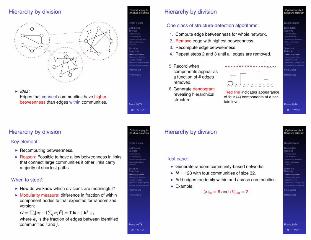
In Fig. 10$c!, we have reduced the network to only thegroups. In this panel, we have drawn each group as a circle,
with size varying roughly with the number of individuals in
the group. The lines between groups indicate collaborations
between group members, with the thickness of the lines
varying in proportion to the number of pairs of scientists
who have collaborated. Now the overall structure of the net-
work becomes easy to see. The network is centered around
the large group in the middle $which consists of researchersprimarily in southern Europe!, with a knot of intercommu-nity collaborations going on between the groups on the lower
right of the picture $mostly Boston University physicists and
FIG. 8. The network of friendships between individuals in the
karate club study of Zachary "36#. The administrator and the in-structor are represented by nodes 1 and 33, respectively. Shaded
squares represent individuals who ended up aligning with the club’s
administrator after the fission of the club, open circles those who
aligned with the instructor.
FINDING AND EVALUATING COMMUNITY STRUCTURE . . . PHYSICAL REVIEW E 69, 026113 $2004!
026113-9
s Zachary’s karate club [25, 16]
I The issue:how do we elucidatethe internal structureof large networksacross many scales?
I Possible substructures:hierarchies, cliques, rings, . . .
I Plus:All combinations of substructures.
I Much focus on hierarchies...
Optimal supply &Structure detection
Single Source
DistributedSourcesFacility location
Size-density law
A reasonable derivation
Global redistributionnetworks
StructureDetectionHierarchy by division
Hierarchy by shuffling
Spectral methods
Hierarchies & Missing Links
General structure detection
Final words
References
Frame 37/78
Hierarchy by division
Top down:
I Idea: Identify global structure first and recursivelyuncover more detailed structure.
I Basic objective: find dominant components that havesignificantly more links within than without, ascompared to randomized version.
I Following comes from “Finding and evaluatingcommunity structure in networks” by Newman andGirvan (PRE, 2004). [16]
I See also1. “Scientific collaboration networks. II. Shortest paths,
weighted networks, and centrality” by Newman (PRE,2001). [14, 15]
2. “Community structure in social and biologicalnetworks” by Girvan and Newman (PNAS, 2002). [9]
Optimal supply &Structure detection
Single Source
DistributedSourcesFacility location
Size-density law
A reasonable derivation
Global redistributionnetworks
StructureDetectionHierarchy by division
Hierarchy by shuffling
Spectral methods
Hierarchies & Missing Links
General structure detection
Final words
References
Frame 38/78
Hierarchy by division
Finding and evaluating community structure in networks
M. E. J. Newman1,2 and M. Girvan2,31Department of Physics and Center for the Study of Complex Systems, University of Michigan, Ann Arbor, Michigan 48109-1120, USA
2Santa Fe Institute, 1399 Hyde Park Road, Santa Fe, New Mexico 87501, USA3Department of Physics, Cornell University, Ithaca, New York 14853-2501, USA
!Received 19 August 2003; published 26 February 2004"
We propose and study a set of algorithms for discovering community structure in networks—natural divi-
sions of network nodes into densely connected subgroups. Our algorithms all share two definitive features:
first, they involve iterative removal of edges from the network to split it into communities, the edges removed
being identified using any one of a number of possible ‘‘betweenness’’ measures, and second, these measures
are, crucially, recalculated after each removal. We also propose a measure for the strength of the community
structure found by our algorithms, which gives us an objective metric for choosing the number of communities
into which a network should be divided. We demonstrate that our algorithms are highly effective at discovering
community structure in both computer-generated and real-world network data, and show how they can be used
to shed light on the sometimes dauntingly complex structure of networked systems.
DOI: 10.1103/PhysRevE.69.026113 PACS number!s": 89.75.Hc, 87.23.Ge, 89.20.Hh, 05.10.!a
I. INTRODUCTION
Empirical studies and theoretical modeling of networks
have been the subject of a large body of recent research in
statistical physics and applied mathematics #1–4$. Networkideas have been applied with success to topics as diverse asthe Internet and the world wide web #5–7$, epidemiology#8–11$, scientific citation and collaboration #12,13$, metabo-lism #14,15$, and ecosystems #16,17$, to name but a few. Aproperty that seems to be common to many networks is com-munity structure, the division of network nodes into groupswithin which the network connections are dense, but be-tween which they are sparser—see Fig. 1. The ability to findand analyze such groups can provide invaluable help in un-derstanding and visualizing the structure of networks. In thispaper, we show how this can be achieved.The study of community structure in networks has a long
history. It is closely related to the ideas of graph partitioningin graph theory and computer science, and hierarchical clus-tering in sociology #18,19$. Before presenting our own find-ings, it is worth reviewing some of this preceding work tounderstand its achievements and shortcomings.Graph partitioning is a problem that arises in, for ex-
ample, parallel computing. Suppose we have a number n ofintercommunicating computer processes, which we wish todistribute over a number g of computer processors. Processesdo not necessarily need to communicate with all others, andthe pattern of required communications can be represented asa graph or network in which the vertices represent processesand edges join process pairs that need to communicate. Theproblem is to allocate the processes to processors in such away as roughly to balance the load on each processor, whileat the same time minimizing the number of edges that runbetween processors, so that the amount of interprocessorcommunication !which is normally slow" is minimized. Ingeneral, finding an exact solution to a partitioning task of thiskind is believed to be an NP-hard problem, making it pro-hibitively difficult to solve exactly for large graphs, but awide variety of heuristic algorithms have been developed
that give acceptably good solutions in many cases, the bestknown being perhaps the Kernighan-Lin algorithm #20$,which runs in time O(n3) on sparse graphs.A solution to the graph partitioning problem is, however,
not particularly helpful for analyzing and understanding net-works in general. If we merely want to find if and how agiven network breaks down into communities, we probablydo not know how many such communities there are going tobe, and there is no reason why they should be roughly thesame size. Furthermore, the number of intercommunityedges need not be strictly minimized either, since more suchedges are admissible between large communities than be-tween small ones.As far as our goals in this paper are concerned, a more
useful approach is that taken by social network analysis withthe set of techniques known as hierarchical clustering. Thesetechniques are aimed at discovering natural divisions of !so-cial" networks into groups, based on various metrics of simi-larity or strength of connection between vertices. They fallinto two broad classes, agglomerative and divisive #19$, de-pending on whether they focus on the addition or removal ofedges to or from the network. In an agglomerative method,similarities are calculated by one method or another betweenvertex pairs, and edges are then added to an initially empty
FIG. 1. A small network with community structure of the type
considered in this paper. In this case there are three communities,
denoted by the dashed circles, which have dense internal links but
between which there is only a lower density of external links.
PHYSICAL REVIEW E 69, 026113 !2004"
1063-651X/2004/69!2"/026113!15"/$22.50 ©2004 The American Physical Society69 026113-1
I Idea:Edges that connect communities have higherbetweenness than edges within communities.
Optimal supply &Structure detection
Single Source
DistributedSourcesFacility location
Size-density law
A reasonable derivation
Global redistributionnetworks
StructureDetectionHierarchy by division
Hierarchy by shuffling
Spectral methods
Hierarchies & Missing Links
General structure detection
Final words
References
Frame 39/78
Hierarchy by division
One class of structure-detection algorithms:
1. Compute edge betweenness for whole network.2. Remove edge with highest betweenness.3. Recompute edge betweenness4. Repeat steps 2 and 3 until all edges are removed.
5 Record whencomponents appear asa function of # edgesremoved.
6 Generate dendogramrevealing hierarchicalstructure.
network !n vertices with no edges" starting with the vertexpairs with highest similarity. The procedure can be halted at
any point, and the resulting components in the network are
taken to be the communities. Alternatively, the entire pro-
gression of the algorithm from empty graph to complete
graph can be represented in the form of a tree or dendrogram
such as that shown in Fig. 2. Horizontal cuts through the tree
represent the communities appropriate to different halting
points.
Agglomerative methods based on a wide variety of simi-
larity measures have been applied to different networks.
Some networks have natural similarity metrics built in. For
example, in the widely studied network of collaborations be-
tween film actors #21,22$, in which two actors are connectedif they have appeared in the same film, one could quantify
similarity by how many films actors have appeared in to-
gether #23$. Other networks have no natural metric, but suit-able ones can be devised using correlation coefficients, path
lengths, or matrix methods. A well known example of an
agglomerative clustering method is the Concor algorithm of
Breiger et al. #24$.Agglomerative methods have their problems, however.
One concern is that they fail with some frequency to find the
correct communities in networks where the community
structure is known, which makes it difficult to place much
trust in them in other cases. Another is their tendency to find
only the cores of communities and leave out the periphery.
The core nodes in a community often have strong similarity,
and hence are connected early in the agglomerative process,
but peripheral nodes that have no strong similarity to others
tend to get neglected, leading to structures like that shown in
Fig. 3. In this figure, there are a number of peripheral nodes
whose community membership is obvious to the eye—in
most cases, they have only a single link to a specific
community—but agglomerative methods often fail to place
such nodes correctly.
In this paper, therefore, we focus on divisive methods.
These methods have been relatively little studied in the pre-
vious literature, either in social network theory or elsewhere,
but, as we will see, they seem to offer a lot of promise. In a
divisive method, we start with the network of interest and
attempt to find the least similar connected pairs of vertices
and then remove the edges between them. By doing this
repeatedly, we divide the network into smaller and smaller
components, and again we can stop the process at any stage
and take the components at that stage to be the network
communities. Again, the process can be represented as a den-
drogram depicting the successive splits of the network into
smaller and smaller groups.
The approach we take follows roughly these lines, but
adopts a somewhat different philosophical viewpoint. Rather
than looking for the most weakly connected vertex pairs, our
approach will be to look for the edges in the network that are
most ‘‘between’’ other vertices, meaning that the edge is, in
some sense, responsible for connecting many pairs of others.
Such edges need not be weak at all in the similarity sense.
How this idea works out in practice will become clear in the
course of the presentation.
Briefly then, the outline of this paper is as follows. In Sec.
II we describe the crucial concepts behind our methods for
finding community structure in networks and show how
these concepts can be turned into a concrete prescription for
performing calculations. In Sec. III we describe in detail the
implementation of our methods. In Sec. IV we consider ways
of determining when a particular division of a network into
communities is a good one, allowing us to quantify the suc-
cess of our community-finding algorithms. And in Sec. V we
give a number of applications of our algorithms to particular
networks, both real and artificial. In Sec. VI we give our
conclusions. A brief report of some of the work contained in
this paper has appeared previously as Ref. #25$.
II. FINDING COMMUNITIES IN A NETWORK
In this paper, we present a class of new algorithms for
network clustering, i.e., the discovery of community struc-
ture in networks. Our discussion focuses primarily on net-
works with only a single type of vertex and a single type of
undirected, unweighted edge, although generalizations to
more complicated network types are certainly possible.
There are two central features that distinguish our algo-
rithms from those that have preceded them. First, our algo-
FIG. 2. A hierarchical tree or dendrogram illustrating the type of
output generated by the algorithms described here. The circles at the
bottom of the figure represent the individual vertices of the net-
work. As we move up the tree, the vertices join together to form
larger and larger communities, as indicated by the lines, until we
reach the top, where all are joined together in a single community.
Alternatively, the dendrogram depicts an initially connected net-
work splitting into smaller and smaller communities as we go from
top to bottom. A cross section of the tree at any level, such as that
indicated by the dotted line, will give the communities at that level.
The vertical height of the split points in the tree are indicative only
of the order in which the splits !or joins" take place, although it ispossible to construct more elaborate dendrograms in which these
heights contain other information.
FIG. 3. Agglomerative clustering methods are typically good at
discovering the strongly linked cores of communities !bold verticesand edges" but tend to leave out peripheral vertices, even when, ashere, most of them clearly belong to one community or another.
M. E. J. NEWMAN AND M. GIRVAN PHYSICAL REVIEW E 69, 026113 !2004"
026113-2
Red line indicates appearanceof four (4) components at a cer-tain level.
Optimal supply &Structure detection
Single Source
DistributedSourcesFacility location
Size-density law
A reasonable derivation
Global redistributionnetworks
StructureDetectionHierarchy by division
Hierarchy by shuffling
Spectral methods
Hierarchies & Missing Links
General structure detection
Final words
References
Frame 40/78
Hierarchy by division
Key element:
I Recomputing betweenness.I Reason: Possible to have a low betweenness in links
that connect large communities if other links carrymajority of shortest paths.
When to stop?:
I How do we know which divisions are meaningful?I Modularity measure: difference in fraction of within
component nodes to that expected for randomizedversion:Q =
∑i [eii − (
∑j eij)
2] = TrE− ||E2||1,where eij is the fraction of edges between identifiedcommunities i and j .
Optimal supply &Structure detection
Single Source
DistributedSourcesFacility location
Size-density law
A reasonable derivation
Global redistributionnetworks
StructureDetectionHierarchy by division
Hierarchy by shuffling
Spectral methods
Hierarchies & Missing Links
General structure detection
Final words
References
Frame 41/78
Hierarchy by division
Test case:I Generate random community-based networks.I N = 128 with four communities of size 32.I Add edges randomly within and across communities.I Example:
〈k〉in = 6 and 〈k〉out = 2.

Optimal supply &Structure detection
Single Source
DistributedSourcesFacility location
Size-density law
A reasonable derivation
Global redistributionnetworks
StructureDetectionHierarchy by division
Hierarchy by shuffling
Spectral methods
Hierarchies & Missing Links
General structure detection
Final words
References
Frame 42/78
Hierarchy by division
A. Tests on computer-generated networks
First, as a controlled test of how well our algorithms per-
form, we have generated networks with known community
structure, to see if the algorithms can recognize and extract
this structure.
We have generated a large number of graphs with n
!128 vertices, divided into four communities of 32 verticeseach. Edges were placed independently at random between
vertex pairs with probability p in for an edge to fall between
vertices in the same community and pout to fall between ver-
tices in different communities. The values of p in and poutwere chosen to make the expected degree of each vertex
equal to 16. In Fig. 6, we show a typical dendrogram from
the analysis of such a graph using the shortest-path between-
ness version of our algorithm. !In fact, for the sake of clarity,the figure is for a 64-node version of the graph." Results forthe random-walk version are similar. At the right of the fig-
ure we also show the modularity, Eq. !5", for the same cal-culation, plotted as a function of position in the dendrogram.
That is, the plot is aligned with the dendrogram so that one
can read off modularity values for different divisions of the
network directly. As we can see, the modularity has a single
clear peak at the point where the network breaks into four
communities, as we would expect. The peak value is around
0.5, which is typical.
In Fig. 7, we show the fraction of vertices in our
computer-generated network sample classified correctly into
the four communities by our algorithms, as a function of the
mean number zout of edges from each vertex to vertices in
other communities. As the figure shows, both the shortest-
path and random-walk versions of the algorithm perform ex-
cellently, with more than 90% of all vertices classified cor-
rectly from zout!0 all the way to around zout!6. Only forzout"6 does the classification begin to deteriorate markedly.In other words, our algorithm correctly identifies the com-
munity structure in the network almost all the way to the
point zout!8 at which each vertex has on average the same
number of connections to vertices outside its community as it
does to those inside.
The shortest-path version of the algorithm does, however,
perform noticeably better than the random-walk version, es-
pecially for the more difficult cases where zout is large. Given
that the random-walk algorithm is also more computationally
demanding, there seems little reason to use it rather than the
shortest-path algorithm, and hence, as discussed previously,
we recommend the latter for most applications. !To be fair,the random-walk algorithm does slightly outperform the
shortest-path algorithm in the example addressed in the fol-
lowing section, although, being only a single case, it is hard
FIG. 6. Plot of the modularity and dendrogram for a 64-vertex random community-structured graph generated as described in the text
with, in this case, z in!6 and zout!2. The shapes at the bottom denote the four communities in the graph and, as we can see, the peak in themodularity !dotted line" corresponds to a perfect identification of the communities.
FIG. 7. The fraction of vertices correctly identified by our algo-
rithms in the computer-generated graphs described in the text. The
two curves show results for the shortest-path !circles" and random-walk !squares" versions of the algorithm as a function of the num-
ber of edges the vertices have to others outside their own commu-
nity. The point zout!8 at the rightmost edge of the plot representsthe point at which vertices have as many connections outside their
own community as inside it. Each data point is an average over 100
graphs.
M. E. J. NEWMAN AND M. GIRVAN PHYSICAL REVIEW E 69, 026113 !2004"
026113-8
I Maximum modularity Q ' 0.5 obtained when fourcommunities are uncovered.
I Further ‘discovery’ of internal structure is somewhatmeaningless, as any communities arise accidentally.
Optimal supply &Structure detection
Single Source
DistributedSourcesFacility location
Size-density law
A reasonable derivation
Global redistributionnetworks
StructureDetectionHierarchy by division
Hierarchy by shuffling
Spectral methods
Hierarchies & Missing Links
General structure detection
Final words
References
Frame 43/78
Hierarchy by division
to know whether this is significant.!
B. Zachary’s karate club network
We now turn to applications of our methods to real-world
network data. Our first such example is taken from one of the
classic studies in social network analysis. Over the course of
two years in the early 1970s, Wayne Zachary observed social
interactions between the members of a karate club at an
American university "36#. He constructed networks of tiesbetween members of the club based on their social interac-
tions both within the club and outside it. By chance, a dis-
pute arose during the course of his study between the club’s
administrator and its principal karate teacher over whether to
raise club fees, and as a result the club eventually split in
two, forming two smaller clubs, centered around the admin-
istrator and the teacher.
In Fig. 8, we show a consensus network structure ex-
tracted from Zachary’s observations before the split. Feeding
this network into our algorithms, we find the results shown in
Fig. 9. In the leftmost two panels, we show the dendrograms
generated by the shortest-path and random-walk versions of
our algorithm, along with the modularity measures for the
same. As we see, both algorithms give reasonably high val-
ues for the modularity when the network is split into two
communities—around 0.4 in each case—indicating that there
is a strong natural division at this level. What is more, the
divisions in question correspond almost perfectly to the ac-
tual divisions in the club revealed by which group each club
member joined after the club split up. $The shapes of thevertices representing the two factions are the same as those
of Fig. 8.! Only one vertex, vertex 3, is misclassified by theshortest-path version of the method, and none are misclassi-
fied by the random-walk version—the latter gets a perfect
score on this test. $On the other hand, the two-communitysplit fails to produce a local maximum in the modularity for
the random-walk method, unlike the shortest-path method,
for which there is a local maximum precisely at this point.!
In the last panel of Fig. 9, we show the dendrogram and
modularity for an algorithm based on shortest-path between-
ness but without the crucial recalculation step discussed in
Sec. II. As the figure shows, without this step, the algorithm
fails to find the division of the network into the two known
groups. Furthermore, the modularity does not reach nearly
such high values as in the first two panels, indicating that the
divisions suggested are much poorer than in the cases with
the recalculation.
C. Collaboration network
For our next example, we look at a collaboration network
of scientists. Figure 10$a! shows the largest component of anetwork of collaborations between physicists who conduct
research on networks. $The authors of the present paper, forinstance, are among the nodes in this network.! This network$which appeared previously in Ref. "37#! was constructed bytaking names of authors appearing in the lengthy bibliogra-
phy of Ref. "4# and cross-referencing with the Physics e-printArchive at arxiv.org, specifically the condensed-matter sec-
tion of the archive, where, for historical reasons, most papers
on networks have appeared. Authors appearing in both were
added to the network as vertices, and edges between them
indicate coauthorship of one or more papers appearing in the
archive. Thus the collaborative ties represented in the figure
are not limited to papers on topics concerning networks—we
were interested primarily in whether people know one an-
other, and collaboration on any topic is a reasonable indica-
tor of acquaintance.
The network as presented in Fig. 10$a! is difficult to in-terpret. Given the names of the scientists, knowledgeable
readers with too much time on their hands could, no doubt,
pick out known groupings, for instance at particular institu-
tions, from the general confusion. But were this a network
about which we had no a priori knowledge, we would be
hard pressed to understand its underlying structure.
Applying the shortest-path version of our algorithm to this
network, we find that the modularity, Eq. $5!, has a strongpeak at 13 communities with a value of Q!0.72"0.02. Ex-tracting the communities from the corresponding dendro-
gram, we have indicated them with colors in Fig. 10$b!. Theknowledgeable reader will again be able to discern known
groups of scientists in this rendering, and more easily now
with the help of the colors. Still, however, the structure of the
network as a whole and of the interactions between groups is
quite unclear.
In Fig. 10$c!, we have reduced the network to only thegroups. In this panel, we have drawn each group as a circle,
with size varying roughly with the number of individuals in
the group. The lines between groups indicate collaborations
between group members, with the thickness of the lines
varying in proportion to the number of pairs of scientists
who have collaborated. Now the overall structure of the net-
work becomes easy to see. The network is centered around
the large group in the middle $which consists of researchersprimarily in southern Europe!, with a knot of intercommu-nity collaborations going on between the groups on the lower
right of the picture $mostly Boston University physicists and
FIG. 8. The network of friendships between individuals in the
karate club study of Zachary "36#. The administrator and the in-structor are represented by nodes 1 and 33, respectively. Shaded
squares represent individuals who ended up aligning with the club’s
administrator after the fission of the club, open circles those who
aligned with the instructor.
FINDING AND EVALUATING COMMUNITY STRUCTURE . . . PHYSICAL REVIEW E 69, 026113 $2004!
026113-9
I Factions in Zachary’s karate club network. [25]
Optimal supply &Structure detection
Single Source
DistributedSourcesFacility location
Size-density law
A reasonable derivation
Global redistributionnetworks
StructureDetectionHierarchy by division
Hierarchy by shuffling
Spectral methods
Hierarchies & Missing Links
General structure detection
Final words
References
Frame 44/78
Betweenness for electrons:
separate component of the graph. Let Vi be the voltage at
vertex i, measured relative to any convenient point. Then for
all i we have
!jAi j"Vi!V j#"$ is!$ it , "1#
where Ai j is the ij element of the adjacency matrix of the
graph, i.e., Ai j"1 if i and j are connected by an edge andAi j"0 otherwise. The left-hand side of Eq. "1# represents thenet current flow out of vertex i along edges of the network,
and the right-hand side represents the source and sink. De-
fining ki"! jAi j , which is the vertex degree, and creating a
diagonal matrix D with these degrees on the diagonal Dii
"ki , this equation can be written in matrix form as (D
!A)•V"s, where the source vector s has components
si"! #1 for i"s
!1 for i"t
0 otherwise.
"2#
We cannot directly invert the matrix D!A to get the volt-age vector V, because the matrix "which is just the graphLaplacian# is singular. This is equivalent to saying that thereis one undetermined degree of freedom corresponding to the
choice of reference potential for measuring the voltages. We
can add any constant to a solution for the vertex voltages and
get another solution—only the voltage differences matter. In
choosing the reference potential, we fix this degree of free-
dom, leaving only n!1 more to be determined. In math-ematical terms, once any n!1 of the equations in our matrixformulation are satisfied, the remaining one is also automati-
cally satisfied so long as current is conserved in the network
as a whole, i.e., so long as ! is i"0, which is clearly true inthis case.
Choosing any vertex v to be the reference point, there-
fore, we remove the row and column corresponding to that
vertex from D and A before inverting. Denoting the resulting
(n!1)$(n!1) matrices Dv and Av , we can then write
V""Dv!Av#!1•s. "3#
Calculation of the currents in the network thus involves
inverting Dv!Av once for any convenient choice of v , and
taking the differences of pairs of columns to get the voltage
vector V for each possible source/sink pair. "The voltage forthe one missing vertex v is always zero, by hypothesis.# Theabsolute magnitudes of the differences of voltages along
each edge give us betweenness scores for the given source
and sink. Summing over all sources and sinks, we then get
our complete betweenness score.
The matrix inversion takes time O(n3) in the worst case,
while the subsequent calculation of betweennesses takes time
O(mn2), where as before m is the number of edges and n the
number of vertices in the graph. Thus, the entire community
structure algorithm, including the recalculation step, will
take O„(n#m)mn2… time to complete, or O(n4) on a sparsegraph. Although, as we will see, the algorithm is good at
finding community structure, this poor performance makes it
practical only for smaller graphs; a few hundreds of vertices
is the most that we have been able to do. It is for this reason
that we recommend using the shortest-path betweenness al-
gorithm in most cases, which gives results about as good or
better with considerably less effort.
C. Random walks
The random-walk betweenness described in Sec. II re-
quires us to calculate how often on average random walks
starting at vertex s will pass down a particular edge from
vertex v to vertex w "or vice versa# before finding their wayto a given target vertex t. To calculate this quantity, we pro-
ceed as follows for each separate component of the graph.
As before, let Ai j be an element of the adjacency matrix
such that Ai j"1 if vertices i and j are connected by an edgeand Ai j"0 otherwise. Consider a random walk that on each
step decides uniformly between the neighbors of the current
vertex j and takes a step to one of them. The number of
neighbors is just the degree of the vertex k j"! iAi j , and the
probability for the transition from j to i is Ai j /k j , which we
can regard as an element of the matrixM"A•D!1, where D
is the diagonal matrix with Dii"ki .
We are interested in walks that terminate when they reach
the target t, so that t is an absorbing state. The most conve-
nient way to represent this is just to remove entirely the
vertex t from the graph, so that no walk ever reaches any
other vertex from t. Thus let Mt"At•Dt!1 be the matrix Mwith the tth row and column removed "and similarly for Atand Dt).
Now the probability that a walk starts at s, takes n steps,
and ends up at some other vertex "not t# is given by the iselement of Mt
n , which we denote %Mtn& is . In particular,
walks end up at v and w with probabilities %Mtn&vs and
%Mtn&ws , and of those a fraction 1/kv and 1/kw , respectively,
then pass along the edge (v ,w) in one direction or the other,assuming such an edge exists. "Note that they may also havepassed along this edge an arbitrary number of times before
reaching this point.# Summing over all n, the mean numberof times that a walk of any length traverses the edge from vto w is kv
!1%(I!Mt)!1&vs , and similarly for walks that go
from w to v .To highlight the similarity with the current-flow between-
ness of Sec. III B, let us denote these two numbers Vv and
FIG. 5. An example of the type of resistor network considered
here, in which a unit resistance is placed on each edge and unit
current flows into and out of the source and sink vertices.
M. E. J. NEWMAN AND M. GIRVAN PHYSICAL REVIEW E 69, 026113 "2004#
026113-6
I Unit resistors on each edge.I For every pair of nodes s
(source) and t (sink), set upunit currents in at s and out att .
I Measure absolute currentalong each edge `, |I`,st |.
I Sum |I`,st | over all pairs of nodes to obtain electronicbetweenness for edge `.
I (Equivalent to random walk betweenness.)I Electronic betweenness for edge between nodes i
and j :B elec
ij = aij |Vi − Vj |.
I Upshot: specific measure of betweenness not tooimportant.
Optimal supply &Structure detection
Single Source
DistributedSourcesFacility location
Size-density law
A reasonable derivation
Global redistributionnetworks
StructureDetectionHierarchy by division
Hierarchy by shuffling
Spectral methods
Hierarchies & Missing Links
General structure detection
Final words
References
Frame 45/78
Scientists working on networks
FIG. 10. Illustration of the use of the community-structure algorithm to make sense of a complex network. !a" The initial network is anetwork of coauthorships between physicists who have published on topics related to networks. The figure shows only the largest component
of the network, which contains 145 scientists. There are 90 more scientists in smaller components, which are not shown. !b" Application ofthe shortest-path betweenness version of the community-structure algorithm produces the communities indicated by the shades of the
vertices. !c" A coarse-graining of the network in which each community is represented by a single node, with edges representing collabo-rations between communities. The thickness of the edges is proportional to the number of pairs of collaborators between communities.
Clearly panel !c" reveals much that is not easily seen in the original network of panel !a".
FINDING AND EVALUATING COMMUNITY STRUCTURE . . . PHYSICAL REVIEW E 69, 026113 !2004"
026113-11
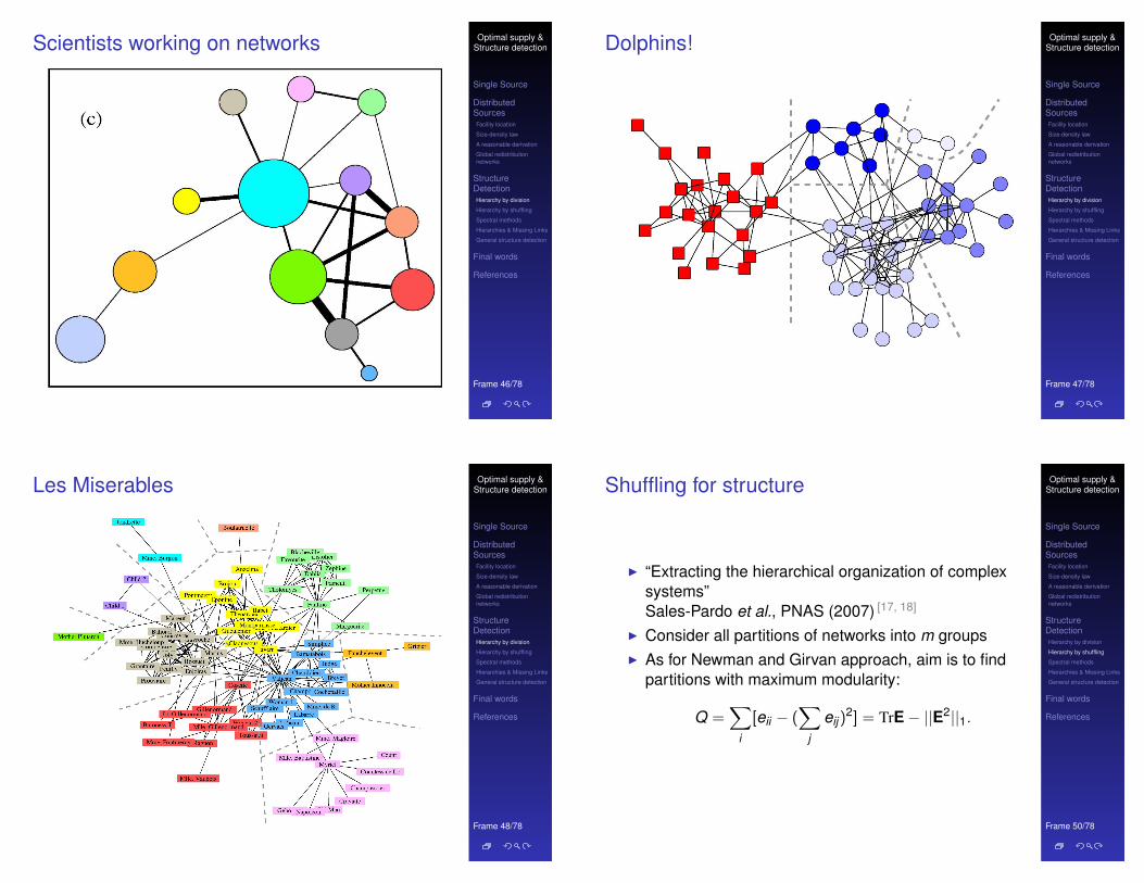
Optimal supply &Structure detection
Single Source
DistributedSourcesFacility location
Size-density law
A reasonable derivation
Global redistributionnetworks
StructureDetectionHierarchy by division
Hierarchy by shuffling
Spectral methods
Hierarchies & Missing Links
General structure detection
Final words
References
Frame 46/78
Scientists working on networks
FIG. 10. Illustration of the use of the community-structure algorithm to make sense of a complex network. !a" The initial network is anetwork of coauthorships between physicists who have published on topics related to networks. The figure shows only the largest component
of the network, which contains 145 scientists. There are 90 more scientists in smaller components, which are not shown. !b" Application ofthe shortest-path betweenness version of the community-structure algorithm produces the communities indicated by the shades of the
vertices. !c" A coarse-graining of the network in which each community is represented by a single node, with edges representing collabo-rations between communities. The thickness of the edges is proportional to the number of pairs of collaborators between communities.
Clearly panel !c" reveals much that is not easily seen in the original network of panel !a".
FINDING AND EVALUATING COMMUNITY STRUCTURE . . . PHYSICAL REVIEW E 69, 026113 !2004"
026113-11
Optimal supply &Structure detection
Single Source
DistributedSourcesFacility location
Size-density law
A reasonable derivation
Global redistributionnetworks
StructureDetectionHierarchy by division
Hierarchy by shuffling
Spectral methods
Hierarchies & Missing Links
General structure detection
Final words
References
Frame 47/78
Dolphins!
group splitting is included also.
The split into two groups appears to correspond to a
known division of the dolphin community !39". Lusseau re-ports that for a period of about two years during observation
of the dolphins they separated into two groups along the
lines found by our analysis, apparently because of the disap-
pearance of individuals on the boundary between the groups.
When some of these individuals later reappeared, the two
halves of the network joined together once more. As Lusseau
points out, developments of this kind illustrate that the dol-
phin network is not merely a scientific curiosity but, like
human social networks, is closely tied to the evolution of the
community. The subgroupings within the larger half of the
network also seem to correspond to real divisions among the
animals: the largest subgroup consists almost of entirely of
females and the others almost entirely of males, and it is
conjectured that the split between the male groups is gov-
erned by matrilineage !D. Lusseau #personal communica-tion$".Figure 12 shows the community structure of the network
of interactions between major characters in Victor Hugo’s
sprawling novel of crime and redemption in post-restoration
FIG. 11. Community structure in the bottlenose dolphins of
Doubtful Sound !38,39", extracted using the shortest-path version ofour algorithm. The squares and circles denote the primary split of
the network into two groups, and the circles are subdivided further
into four smaller groups as shown. The modularity for the split is
Q!0.52. The network has been drawn with longer edges betweenvertices in different communities than between those in the same
community, to make the community groupings clearer. The same is
also true of Figs. 12 and 13.
FIG. 12. The network of interactions between major characters in the novel Les Miserables by Victor Hugo. The greatest modularity
achieved in the shortest-path version of our algorithm is Q!0.54 and corresponds to the 11 communities shown.
M. E. J. NEWMAN AND M. GIRVAN PHYSICAL REVIEW E 69, 026113 #2004$
026113-12
Optimal supply &Structure detection
Single Source
DistributedSourcesFacility location
Size-density law
A reasonable derivation
Global redistributionnetworks
StructureDetectionHierarchy by division
Hierarchy by shuffling
Spectral methods
Hierarchies & Missing Links
General structure detection
Final words
References
Frame 48/78
Les Miserables
group splitting is included also.
The split into two groups appears to correspond to a
known division of the dolphin community !39". Lusseau re-ports that for a period of about two years during observation
of the dolphins they separated into two groups along the
lines found by our analysis, apparently because of the disap-
pearance of individuals on the boundary between the groups.
When some of these individuals later reappeared, the two
halves of the network joined together once more. As Lusseau
points out, developments of this kind illustrate that the dol-
phin network is not merely a scientific curiosity but, like
human social networks, is closely tied to the evolution of the
community. The subgroupings within the larger half of the
network also seem to correspond to real divisions among the
animals: the largest subgroup consists almost of entirely of
females and the others almost entirely of males, and it is
conjectured that the split between the male groups is gov-
erned by matrilineage !D. Lusseau #personal communica-tion$".Figure 12 shows the community structure of the network
of interactions between major characters in Victor Hugo’s
sprawling novel of crime and redemption in post-restoration
FIG. 11. Community structure in the bottlenose dolphins of
Doubtful Sound !38,39", extracted using the shortest-path version ofour algorithm. The squares and circles denote the primary split of
the network into two groups, and the circles are subdivided further
into four smaller groups as shown. The modularity for the split is
Q!0.52. The network has been drawn with longer edges betweenvertices in different communities than between those in the same
community, to make the community groupings clearer. The same is
also true of Figs. 12 and 13.
FIG. 12. The network of interactions between major characters in the novel Les Miserables by Victor Hugo. The greatest modularity
achieved in the shortest-path version of our algorithm is Q!0.54 and corresponds to the 11 communities shown.
M. E. J. NEWMAN AND M. GIRVAN PHYSICAL REVIEW E 69, 026113 #2004$
026113-12
Optimal supply &Structure detection
Single Source
DistributedSourcesFacility location
Size-density law
A reasonable derivation
Global redistributionnetworks
StructureDetectionHierarchy by division
Hierarchy by shuffling
Spectral methods
Hierarchies & Missing Links
General structure detection
Final words
References
Frame 50/78
Shuffling for structure
I “Extracting the hierarchical organization of complexsystems”Sales-Pardo et al., PNAS (2007) [17, 18]
I Consider all partitions of networks into m groupsI As for Newman and Girvan approach, aim is to find
partitions with maximum modularity:
Q =∑
i
[eii − (∑
j
eij)2] = TrE− ||E2||1.

Optimal supply &Structure detection
Single Source
DistributedSourcesFacility location
Size-density law
A reasonable derivation
Global redistributionnetworks
StructureDetectionHierarchy by division
Hierarchy by shuffling
Spectral methods
Hierarchies & Missing Links
General structure detection
Final words
References
Frame 51/78
Shuffling for structure
I Consider partition network, i.e., the network of allpossible partitions.
I Defn: Two partitions are connected if they differ onlyby the reassignment of a single node.
I Look for local maxima in partition network.I Construct an affinity matrix with entries Aij .I Aij = Pr random walker on modularity network ends
up at a partition with i and j in the same group.I C.f. topological overlap between i and j =
# matching neighbors for i and j divided by maximumof ki and kj .
Optimal supply &Structure detection
Single Source
DistributedSourcesFacility location
Size-density law
A reasonable derivation
Global redistributionnetworks
StructureDetectionHierarchy by division
Hierarchy by shuffling
Spectral methods
Hierarchies & Missing Links
General structure detection
Final words
References
Frame 52/78
Shuffling for structure
Corrections
APPLIED PHYSICAL SCIENCES. For the article ‘‘Extracting thehierarchical organization of complex systems,’’ by MartaSales-Pardo, Roger Guimera, Andre A. Moreira, and LuısA. Nunes Amaral, which appeared in issue 39, September25, 2007, of Proc Natl Acad Sci USA (104:15224–15229; first
published September 19, 2007; 10.1073!pnas.0703740104),the authors note that, due to a printer’s error, Fig. 1Bappeared incorrectly. The corrected figure and its legendappear below. This error does not affect the conclusions ofthe article.
-
Modularity, M0.0
0.5
1.0
P(M
’ > M
)
a
c
d
b
0.0 0.5 1.0
a
b
d
c
Modularity
c
ba
d
Mav
A
B
C
D
E
3
6
13
12
11
15
1410
9
5
8
7
24
1
Fig. 1. Schematic illustration of our method for asimple network. (A) Example network. (B) Modularitylandscape. For the example network, there are 15 dis-tinct groupings of nodes into modules. Each large col-ored circle represents a partition, which we draw insidethe circle, with different colors indicating different mod-ules. For clarity, we label each partition with a numberfrom1to15.Thecolorof thepartitioncircle indicates themodularity of that partition following the color code onthe bottom right-hand side of the diagram. For simplic-ity, we consider only single node changes; thus, we con-nect two partitions, for instance 1 and 2, because thechange of a node to a new module in partition 1 gener-ates partition 2. The arrows show the direction of in-creasing modularity. Local maxima correspond to thosepartitions that do not point to any other partition; thatis, the change of a single node does not increase themodularity. In the example, there are two local maxima:partition 1 and partition 15. To illustrate the concept ofbasin of attraction, we show next to each partition acolored bar (black and white) that represents the prob-ability that a walker that starts from, for instance, partition 2 and only moves to partitions with larger modularity ends up in either of the local maxima. We use whiteto indicate partition 15 and black to indicate partition 1. (C) Coclassification matrix. We show the number of times two nodes are classified in the same module, startingfrom a random partition. Note that nodes a, c and b, d are always classified together because they are in the same module in both local maxima (partitions 1and 15).In contrast, nodes a and b are only in the same module for one of the maxima (partition 1); therefore, the coclassification is lower than one, but larger than zero. (D)Comparison with randomized networks. In this case, this is the only network that one can build keeping the same degree distribution and not allowing for self-loops.Therefore, the average modularity for the local maxima of the randomized networks and that of the network under analysis are the same. Thus, our conclusion is thatthis network has no internal organization. (E) Representation of the hierarchical organization for the example network. We show the ordered coclassification matrixon the Left, and on the Right is the tree showing the organization of the nodes into modules. In this case, the network has no significant structure; thus, we show abar of a single color indicating that there is a single module. Note that a modularity maximization algorithm would have a certain chance (the probability dependingon the specific algorithm) of finding partition 15 as the optimal partition and would thus conclude that the network does have a modular structure.
www.pnas.org!cgi!doi!10.1073!pnas.0709460104
BIOCHEMISTRY. For the article ‘‘A surface on the androgenreceptor that allosterically regulates coactivator binding,’’ by EvaEstebanez-Perpina, Alexander A. Arnold, Phuong Nguyen, Ed-son Delgado Rodrigues, Ellena Mar, Raynard Bateman, PeterPallai, Kevan M. Shokat, John D. Baxter, R. Kiplin Guy, PaulWebb, and Robert J. Fletterick, which appeared in issue 41,October 9, 2007, of Proc Natl Acad Sci USA (104:16074–16079;first published October 2, 2007; 10.1073!pnas.0708036104), theauthor name Alexander A. Arnold should have appeared asLeggy A. Arnold. The online version has been corrected. Thecorrected author line appears below.
Eva Estebanez-Perpina, Leggy A. Arnold, Phuong Nguyen,Edson Delgado Rodrigues, Ellena Mar, Raynard Bateman,Peter Pallai, Kevan M. Shokat, John D. Baxter, R. KiplinGuy, Paul Webb, and Robert J. Fletterick
www.pnas.org!cgi!doi!10.1073!pnas.0709913104
18874 " PNAS " November 20, 2007 " vol. 104 " no. 47 www.pnas.org
I A: Base network; B: Partition network; C:Coclassification matrix; D: Comparison to randomnetworks (all the same!); E: Ordered coclassificationmatrix; Conclusion: no structure...
Optimal supply &Structure detection
Single Source
DistributedSourcesFacility location
Size-density law
A reasonable derivation
Global redistributionnetworks
StructureDetectionHierarchy by division
Hierarchy by shuffling
Spectral methods
Hierarchies & Missing Links
General structure detection
Final words
References
Frame 53/78
Shuffling for structure
I Method obtains a distribution of classificationhierarchies.
I Note: the hierarchy with the highest modularity scoreisn’t chosen.
I Idea is to weight possible hierarchies according totheir basin of attraction’s size in the partition network.
I Next step: Given affinities, now need to sort nodesinto modules, submodules, and so on.
I Idea: permute nodes to minimize following cost
C =1N
N∑i=1
N∑j=1
Aij |i − j |.
I Use simulated annealing (slow).
Optimal supply &Structure detection
Single Source
DistributedSourcesFacility location
Size-density law
A reasonable derivation
Global redistributionnetworks
StructureDetectionHierarchy by division
Hierarchy by shuffling
Spectral methods
Hierarchies & Missing Links
General structure detection
Final words
References
Frame 54/78
Shuffling for structure
Let then Pmax be the set of partitions for which the modularity Mis a local maxima, that is, partitions for which neither the change ofa single node from one module to another nor the merging of twomodules will yield a higher modularity (Fig. 1B). The most straight-forward way to calculate Aij would be to consider all partitions P !Pmax, and find the fraction for which (i, j) are placed in the samemodule. However, such a procedure would not take into consid-eration the size of the basins of attraction of the different maxima.To understand the importance of this fact, consider the ‘‘landscape’’in Fig. 1 in which each node represents a partition of the network,and for simplicity, we connect two partitions if the change of a singlenode transforms one partition into the other. This landscape hastwo local maxima, partitions 1 and 15. Therefore, if we were onlyto consider those partitions, we would conclude that those parti-tions are equally important. However, there is no reason to assumethat all partitions have the same importance. Actually, for networkswith a very clear modular structure, one expects that a few localmaxima will yield the most relevant information about the orga-nization of the network. This idea is can be formalized through theconcept of basin of attraction.
Consider again the landscape in Fig. 1B. Suppose we wanted tofind a partition for which the modularity is a maximum with no apriori information on the landscape. We would start by grouping thenodes into a randomly chosen partition; let us say, partition 13. In
partition 13, nodes a and c are placed in one group, whereas nodesb and d are placed into their own groups. There are two single nodechanges that increase the modularity. Node b can be placed in thesame group as node d; this is partition 15, which is a local maxima.Instead, node b can be placed in the same group as nodes a and c;this is partition 14. Partition 14 is not a modularity maximum; thusone would continue our random ascent of the modularity land-scape. From partition 14, one could move to partition 1 or topartition 15, both local maxima. This example illustrates that frompartition 13, one has a 25% chance of ending in partition 1 and a75% chance of ending in partition 15. If one repeats this calculationfor every possible starting partition, one obtains the size of the basinof attraction of the two local modularity maxima.
Formally, the size of the basin of attraction of P is
b!P" ! !P!P
b!P, P"
"P " [2]
where b(P, P) is the probability that starting from partition P oneends at partition P ! Pmax and !P! is the number of possiblepartitions (Fig. 1B).
We propose that the affinity Aij of a pair of nodes (i, j) is then theprobability that when local maxima partition P ! Pmax are sampledwith probabilities b(P), nodes (i, j) are classified in the same module.
0.8 1 1.20.4 0.5 0.6 0.7 0.8 0.9 10.00.20.40.60.81.0
Mut
ual in
form
atio
n
0.6 0.8 1 1.2 ρ
0.5 1.00.0
B
Co−
affinity determination hierarchical tree determination
classification
Co−classification
clusteringHierarchical
Hierarchicalclustering
Box modelclustering
A
Topological overlap
Fig. 2. Affinity measures and clustering methods. (A)We generate a model network comprised of 640 nodeswith average degree 16 and with a three-level hierarchi-cal structure (see SI Fig. 8 for results for a network with a‘‘flat’’ organization of the nodes). We show the affinitymatrices Aij obtained for two different measures: (i) to-pological overlap (11) and (ii) coclassification (see textand Supplementary Information). The color scale goesfrom red for an affinity of one to dark blue for an affinityof zero. At the far right, we show the hierarchical treeobtained by using two different methods: hierarchicalclustering and the ‘‘box clustering’’ method we propose.In the hierarchical clustering tree, the vertical axis showsthe average distance, dij # 1 " Aij, of the matrix ele-ments that have already merged. In the box-model clus-tering tree, each row corresponds to one hierarchicallevel. Different colors indicate different modules at thatlevel. To better identify which are the submodules at alower level, we color the nodes in the submodules withshades of the color used for the modules in the levelabove. Note that topological overlap fails to find anymodular structure beyond a locally dense connectivitypattern. In contrast, the coclassification measure clearlyreveals the hierarchical organization of the network bythe ‘‘nested-box’’ pattern along the diagonal. Signifi-cantly, thehierarchical treeobtainedviahierarchicalclus-tering fails to reproduce the clear three-level hierarchicalstructure that the affinity matrix displays, whereas thebox-model clustering tree accurately reproduces thethree-level hierarchical organization of the network. (B)Accuracyof themethod.Wegeneratenetworkswith640nodes and with built-in hierarchical structure comprisingone (Left), two (Center), and three (Right) levels. The toplevel always comprises four modules of 160 nodes each.For networks with a second level, each of the top-levelmodules is organized into four submodules of 40 nodes.For the networks with three levels, each level-two mod-ule is further split into four submodules of 10 nodes. Webuild networks with different degrees of level cohesive-ness by tuning a single parameter # (see SI Text). For lowvalues of #, the levels are very cohesive, for high values of# the levels are weakly cohesive. Because we know a priori which are the nodes that should be coclassified at each level, we measure the accuracy as the mutualinformation between the empirical partition of the nodes and the theoretical one (23). We plot the mutual information versus# and, for comparison, we also plot theaccuracy of a standard community detection algorithm (24) in finding the top level of the networks (dashed green line). Each point is the average over 10differentrealizations of the network. Filled circles, empty squares, and filled diamonds represent the accuracy at the top, middle, and lowest levels, respectively. Note that ourmethod isasgoodatdetectingcommunitiesasa standardcommunitydetectionalgorithmfornetworkswithaflatorganizationof thenodes.Additionally,ourmethodis able to detect the top level for all cases analyzed, whereas standard modularity optimization algorithms are not.
15226 # www.pnas.org$cgi$doi$10.1073$pnas.0703740104 Sales-Pardo et al.
I N = 640,I 〈k〉 = 16,I 3 tiered
hierarchy.

Optimal supply &Structure detection
Single Source
DistributedSourcesFacility location
Size-density law
A reasonable derivation
Global redistributionnetworks
StructureDetectionHierarchy by division
Hierarchy by shuffling
Spectral methods
Hierarchies & Missing Links
General structure detection
Final words
References
Frame 55/78
Air transportation:
matrix. As we said previously, we assume that the information atdifferent levels in the hierarchy is decoupled, thus to detectsubmodules beyond the first level, one needs to break the networkinto the subnetworks defined by each module and apply the sameprocedure from the start. The algorithm iterates these steps for eachidentified box until no subnetworks are found to have internalstructure.
Method ValidationWe validate our method on hierarchically nested random graphswith one, two, and three hierarchical levels. We define the accuracyof the method as the mutual information between the empiricalpartition and the theoretical one (23). Fig. 2C shows that thealgorithm uncovers the correct number of levels in the hierarchy.
Moreover, our method always detects the top level, even for thenetworks with three hierarchical levels. In contrast, because thepartition that globally maximizes M corresponds to the submodulesin the second level, even the more accurate module identificationalgorithms based on modularity maximization would fail to capturethe top level organization (20).
The hierarchically nested random graphs considered above havea homogeneous hierarchical structure; however, real-world net-works are not likely to be so regular. In particular, for real-worldnetworks, one expects that some modules will have deeper hierar-chical structures than others. We thus have verified that our methodis also able to correctly uncover the organization of model networkswith heterogeneous hierarchical structures (see SI Fig. 10).
Analysis of Real-World NetworksHaving validated our method, we next analyze different types ofreal-world networks for which we have some insight into thenetwork structure: the worldwide air-transportation network (35–37), an e-mail exchange network of a Catalan university (13), andan electronic circuit (4).
In the air-transportation network, nodes correspond to cities(that is, all airports around major cities would be merged into asingle node), and two nodes are connected if there is a nonstopflight connecting them. In the e-mail network, nodes are people andtwo people are connected if they send e-mails to each other. In theelectronic network, nodes are transistors and two transistors areconnected if the output of one transistor is the input of the other(Table 1).
We find that the air-transportation network is strongly modularand has a deep hierarchical organization (Fig. 3). This finding does
not come as a surprise because historical, economic, political, andgeographical constraints shape the topology of the network (35–37). We find eight main modules that closely match major conti-nents and subcontinents and major political divisions, and thus theytruly represent the highest level of the hierarchy.
The electronic circuit network is comprised of eight D-flip-flopsand 58 logic gates (4). Our method identifies two levels in thenetwork (SI Fig. 12A). At the top level, modules comprise either aD-flip-flop plus some additional gates, or a group of logic gates. Atthe second level, the majority of modules comprise single gates.
For the e-mail network, five of the seven major modules at thetop level (SI Fig. 12B) correspond to schools in the university, with!70% of the nodes in each of those modules affiliated with thecorresponding school. The remaining two major modules at the toplevel are a mixture of schools and administration offices (oftencollocated on campus), which are distinctly separated at the secondlevel. The second level also identifies major departments andgroups within a school, as well as research centers closely related toindividual schools.
Application to Metabolic NetworksFinally, we analyze the metabolic networks of E. coli obtainedfrom three different sources! (Fig. 4 and SI Fig. 13): the KEGGdatabase (40, 41), the Ma-Zeng database (42), and the recon-struction compiled by Palsson’s Systems Biology Laboratory atthe UCSD (43). In these networks, nodes are metabolites andtwo metabolites are connected if there is a reaction thattransforms one into the other (44).
To quantify the plausibility of our classification scheme, weanalyze the within-module consistency of metabolite pathway clas-sification for the top and the second levels of the metabolic networkof E. coli (43). For each module, we first identify the pathwaysrepresented; then, we compute the fraction of metabolites that areclassified in the most abundant pathway. We find that there is aclear correlation between modules and known pathways: At the toplevel, for all of the modules except one (the central metabolism
¶The ability of the present method to detect the top level is significant. A previous studycoauthored by two of us identified 19 modules in the worldwide air-transportationnetwork (37) by using the most accurate modularity maximization algorithm in theliterature (38).
!In the SI Text, we also show the organization obtained for the UCSD reconstruction of themetabolic network for Helicobacter pylori (39).
DC
A B
Fig. 3. Hierarchical organization of the air-transportation network. (A) Global-level af-finity matrix and hierarchical tree (the repre-sentation is the same used in Fig. 2). (B) Top-level modules. Each dot represents a city anddifferent colors represent different modules.Note that the top level in the hierarchy cor-responds to major geopolitical units. (C) The‘‘Eurasian’’module (which is composedof themajority of European countries, ex-SovietUnion countries, Middle-Eastern countries,India, and countries in Northern half of Af-rica) splits for levels ! " 2 into five submod-ules. (D)The ‘‘NearandMiddleEast’’ submod-ule further splits into seven submodules for! " 3 (D). Note that the air-transportationnetwork is large and very dense (Table 1), andthus the organization of the network is not atall apparent (SI Fig. 11). Remarkably, themodules our method detects show a clearagreement with geopolitical units.
15228 " www.pnas.org#cgi#doi#10.1073#pnas.0703740104 Sales-Pardo et al.
I Modules found match up with geopolitical units.
Optimal supply &Structure detection
Single Source
DistributedSourcesFacility location
Size-density law
A reasonable derivation
Global redistributionnetworks
StructureDetectionHierarchy by division
Hierarchy by shuffling
Spectral methods
Hierarchies & Missing Links
General structure detection
Final words
References
Frame 57/78
General structure detection
I “Detecting communities in large networks”Capocci et al. (2005) [4]
I Consider normal matrix K−1A, random walk matrixATK−1, Laplacian K− A, and AAT.
I Basic observation is that eigenvectors associatedwith secondary eigenvalues reveal evidence ofstructure.
I Build on Kleinberg’s HITS algorithm. [13]
Optimal supply &Structure detection
Single Source
DistributedSourcesFacility location
Size-density law
A reasonable derivation
Global redistributionnetworks
StructureDetectionHierarchy by division
Hierarchy by shuffling
Spectral methods
Hierarchies & Missing Links
General structure detection
Final words
References
Frame 58/78
General structure detection
I Example network:
Thus, solving the eigenproblem is equivalent to minimizing function (1) withconstraint (2), where the xi’s are eigenvectors components. The absolute minimumcorresponds to the trivial eigenvector, which is constant. The other stationary pointscorrespond to eigenvectors where components associated to well connected nodesassume similar values.
In order to compute cluster sizes and distribution, methods such as bisection oredge-betweenness based ones are very poor in detecting the end of the recursivesplitting. Our approach, instead, immediately detects the number of clear clustersfrom the eigenvectors profile.
As an illustrative example, we show in Fig. 2 the profile of the second eigenvectorsof D!1W corresponding to the simple graph shown in Fig. 1 with S ¼ 19 nodes,where random weights between 1 and 10 were assigned to the links (Figs. 1 and 2).The components of the eigenvectors assume approximately constant values on nodesbelonging to the same community. Thus, the number of communities emergesnaturally and it is not needed as input.
However, as aforementioned, when dealing with large networks with no clearpartitioning, the precise value of the eigenvector components is of little use. In suchsituations, the typical eigenvector profile is not step-like, but resembles a continuouscurve. Nevertheless, our method can still be applied, and efficiently detects sets ofwell connected nodes. In fact, components corresponding to nodes belonging to thesame communities are still strongly correlated taking, in each eigenvector, similarvalues among themselves. Thus, a natural way to identify communities in anautomatic manner, is to measure the correlation
rij ¼hxixji!h xiihxji
½ðhx2i i!h xii2Þðhx2j i!h xji2Þ&1=2, (4)
where the average h'i is over the first few nontrivial eigenvectors. The quantity rijmeasures the community closeness between nodes i and j: Though the performancemay be improved by averaging over more and more eigenvectors, with increasedcomputational effort, we find that indeed a small number of eigenvectors suffices toidentify the community to which nodes belong, even in large networks.
ARTICLE IN PRESS
Fig. 1. Network employed as an example, with S ¼ 19 and random weights between 1 and 10 assigned tothe links. Three clear clusters appear, composed by nodes 0–6, 7–12 and 13–19.
A. Capocci et al. / Physica A 352 (2005) 669–676672
Optimal supply &Structure detection
Single Source
DistributedSourcesFacility location
Size-density law
A reasonable derivation
Global redistributionnetworks
StructureDetectionHierarchy by division
Hierarchy by shuffling
Spectral methods
Hierarchies & Missing Links
General structure detection
Final words
References
Frame 59/78
General structure detection
I Second eigenvector’s components:
When dealing with a directed network, links do not correspond to any equivalencerelation. Rather, pointing to common neighbors is a significant relation, as suggestedin the sociologists’ literature where this quantity measures the so-called structuralequivalence of nodes [18]. Accordingly, in a directed network, clusters should becomposed by nodes pointing to a high number of common neighbors, no mattertheir direct linkage. For directed networks, we thus modify our method in thestreamline of the HITS algorithm [17]. The HITS algorithm was proposed onempirical bases to find the main communities in large oriented networks. It assumesthat the largest components (in the absolute value) of eigenvectors of the matricesAAT and ATA correspond to highly clustered nodes belonging to a singlecommunity. Such algorithm efficiently detects the main communities, even whenthese are not sharply defined. However, it becomes computationally heavy when oneis interested in minor communities, which correspond to smaller eigenvalues. Asexplained in the undirected case, we tackle this issue by combining information fromthe first few eigenvectors of the normal matrix and extracting the communitystructure from correlations between the same components in different eigenvectors.
To detect the community structure in a directed network, we therefore replace, inthe previous analysis, the matrix W with a matrix Y ¼ WWT: This corresponds toreplacing the directed network with an undirected weighted network, where nodespointing to common neighbors are connected by a link, whose intensity isproportional to the total sum of the weights of the links pointing from the twooriginal nodes to the common neighbors. Then, one performs the analysis on theundirected network as described previously. Thus, the function to minimize in thiscase is
yðxÞ ¼X1;S
ijl
ðxi $ xjÞ2wilwjl . (5)
ARTICLE IN PRESS
Fig. 2. Values of the 2nd eigenvector components for matrix D$1W relative to the graph depictedin Fig. 1.
A. Capocci et al. / Physica A 352 (2005) 669–676 673

Optimal supply &Structure detection
Single Source
DistributedSourcesFacility location
Size-density law
A reasonable derivation
Global redistributionnetworks
StructureDetectionHierarchy by division
Hierarchy by shuffling
Spectral methods
Hierarchies & Missing Links
General structure detection
Final words
References
Frame 61/78
Hierarchies and missing linksClauset et al., Nature (2008) [5]
LETTERS
Hierarchical structure and the prediction of missinglinks in networksAaron Clauset1,3, Cristopher Moore1,2,3 & M. E. J. Newman3,4
Networks have in recent years emerged as an invaluable tool fordescribing and quantifying complex systems in many branches ofscience1–3. Recent studies suggest that networks often exhibit hier-archical organization, in which vertices divide into groups thatfurther subdivide into groups of groups, and so forth overmultiplescales. Inmany cases the groups are found to correspond to knownfunctional units, such as ecological niches in food webs, modulesin biochemical networks (protein interaction networks, metabolicnetworks or genetic regulatory networks) or communities in socialnetworks4–7. Here we present a general technique for inferringhierarchical structure from network data and show that the exist-ence of hierarchy can simultaneously explain and quantitativelyreproduce many commonly observed topological properties ofnetworks, such as right-skewed degree distributions, high cluster-ing coefficients and short path lengths. We further show thatknowledge of hierarchical structure can be used to predict missingconnections in partly known networks with high accuracy, and formore general network structures than competing techniques8.Taken together, our results suggest that hierarchy is a centralorganizing principle of complex networks, capable of offeringinsight into many network phenomena.
Much recent work has been devoted to the study of clustering andcommunity structure in networks5,6,9–11. Hierarchical structure goesbeyond simple clustering, however, by explicitly including organiza-tion at all scales in a network simultaneously. Conventionally, hier-archical structure is represented by a tree, or dendrogram, in whichclosely related pairs of vertices have lowest common ancestors thatare lower in the tree than those of more distantly related pairs (seeFig. 1). We expect the probability of a connection between two ver-tices to depend on their degree of relatedness. Structure of this typecan be modelled mathematically by using a probabilistic approach inwhich we endow each internal node r of the dendrogram with aprobability pr and then connect each pair of vertices for which r isthe lowest common ancestor independently with probability pr(Fig. 1).
This model, which we call a hierarchical random graph, is similarin spirit to (although different in realization from) the tree-basedmodels used in some studies of network search and navigation12,13.Like most work on community structure, it assumes that commu-nities at each level of organization are disjoint. Overlapping com-munities have occasionally been studied (see, for example, ref. 14)and could be represented with a more elaborate probabilistic model;however, as we discuss below, the present model already capturesmany of the structural features of interest.
Given a dendrogram and a set of probabilities pr, the hierarchicalrandom graph model allows us to generate artificial networks with aspecified hierarchical structure, a procedure that might be useful incertain situations. Our goal here, however, is a different one.Wewish
to detect and analyse the hierarchical structure, if any, of networks inthe real world. We accomplish this by fitting the hierarchical modelto observed network data by using the tools of statistical inference,combining a maximum-likelihood approach15 with a Monte Carlosampling algorithm16 on the space of all possible dendrograms. Thistechnique allows us to sample hierarchical random graphs with prob-ability proportional to the likelihood that they generate the observednetwork. To obtain the results described below we combine informa-tion from a large number of such samples, each of which is a rea-sonably likely model of the data.
The success of this approach relies on the flexible nature of ourhierarchical model, which allows us to fit a wide range of networkstructures. The traditional picture of communities or modules in anetwork, for example, corresponds to connections that are densewithin groups of vertices and sparse between them—a behaviourcalled ‘assortativity’ in the literature17. The hierarchical random
1Department of Computer Science, and 2Department of Physics andAstronomy, University of NewMexico, Albuquerque, NewMexico 87131, USA. 3Santa Fe Institute, 1399Hyde ParkRoad, Santa Fe, New Mexico 87501, USA. 4Department of Physics and Center for the Study of Complex Systems, University of Michigan, Ann Arbor, Michigan 48109, USA.
Figure 1 | A hierarchical network with structure on many scales, and thecorresponding hierarchical random graph. Each internal node r of thedendrogram is associated with a probability pr that a pair of vertices in theleft and right subtrees of that node are connected. (The shades of the internalnodes in the figure represent the probabilities.)
Vol 453 | 1 May 2008 |doi:10.1038/nature06830
98Nature Publishing Group©2008
I Idea: Shades indicate probability that nodes in leftand right subtrees of dendogram are connected.
I Handle: Hierarchical random graph models.I Plan: Infer consensus dendogram for a given real
network.I Obtain probability that links are missing (big
problem...).
Optimal supply &Structure detection
Single Source
DistributedSourcesFacility location
Size-density law
A reasonable derivation
Global redistributionnetworks
StructureDetectionHierarchy by division
Hierarchy by shuffling
Spectral methods
Hierarchies & Missing Links
General structure detection
Final words
References
Frame 62/78
Hierarchies and missing links
I Model also predicts reasonably well1. average degree,2. clustering,3. and average shortest path length.
graph can capture behaviour of this kind using probabilities pr thatdecrease as wemove higher up the tree. Conversely, probabilities thatincrease as we move up the tree correspond to ‘disassortative’ struc-tures in which vertices are less likely to be connected on small scalesthan on large ones. By letting the pr values vary arbitrarily throughoutthe dendrogram, the hierarchical random graph can capture bothassortative and disassortative structure, as well as arbitrary mixturesof the two, at all scales and in all parts of the network.
To demonstrate ourmethod we have used it to construct hierarch-ical decompositions of three example networks drawn fromdisparatefields: the metabolic network of the spirochaete Treponema palli-dum18, a network of associations between terrorists19, and a foodweb of grassland species20. To test whether these decompositionsaccurately capture the important structural features of the networks,we use the sampled dendrograms to generate new networks, differentin detail from the originals but, by definition, having similar hier-archical structure (see Supplementary Information for more details).We find that these ‘resampled’ networks match the statistical pro-perties of the originals closely, including their degree distributions,clustering coefficients, and distributions of shortest path lengthsbetween pairs of vertices, despite the fact that none of these propertiesis explicitly represented in the hierarchical random graph (Table 1,and Supplementary Fig. 3). It therefore seems that a network’s hier-archical structure is capable of explaining a wide variety of othernetwork features as well.
The dendrograms produced by our method are also of interest inthemselves, as a graphical representation and summary of the hier-archical structure of the observed network. As discussed above, ourmethod can generate not just a single dendrogram but a set of den-drograms, each of which is a good fit to the data. From this set we can,by using techniques from phylogeny reconstruction21, create a singleconsensus dendrogram, which captures the topological features thatappear consistently across all or a large fraction of the dendrogramsand typically is a better summary of the network’s structure than anyindividual dendrogram. Figure 2a shows such a consensus dendro-gram for the grassland species network, which clearly reveals com-munities and subcommunities of plants, herbivores, parasitoids andhyperparasitoids.
Another application of the hierarchical decomposition is the pre-diction of missing interactions in networks. In many settings, thediscovery of interactions in a network requires significant experi-mental effort in the laboratory or the field. As a result, our currentpictures of many networks are substantially incomplete22–28. Analternative to checking exhaustively for a connection between everypair of vertices in a network is to try to predict, in advance and on thebasis of the connections already observed, which vertices are mostlikely to be connected, so that scarce experimental resources can befocused on testing for those interactions. If our predictions are good,we can in this way substantially reduce the effort required to establishthe network’s topology.
The hierarchical decomposition can be used as the basis for aneffective method of predicting missing interactions as follows.Given an observed but incomplete network, we generate, as describedabove, a set of hierarchical random graphs—dendrograms and theassociated probabilities pr—that fit that network. Then we look forpairs of vertices that have a high average probability of connectionwithin these hierarchical random graphs but are unconnected in the
observed network. These pairs we consider themost likely candidatesformissing connections. (Technical details of the procedure are givenin Supplementary Information.)
We demonstrate the method by using our three example networksagain. For each network we remove a subset of connections chosenuniformly at random and then attempt to predict, on the basis of theremaining connections, which have been removed. A standardmetricfor quantifying the accuracy of prediction algorithms, commonlyused in the medical and machine learning communities, is theAUC statistic, which is equivalent to the area under the receiveroperating characteristic (ROC) curve29. In the present context, theAUC statistic can be interpreted as the probability that a randomlychosenmissing connection (a true positive) is given a higher score byour method than a randomly chosen pair of unconnected vertices (atrue negative). Thus, the degree to which the AUC exceeds 0.5 indi-cates how much better our predictions are than chance. Figure 2shows the AUC statistic for the three networks as a function of thefraction of the connections known to the algorithm. For all threenetworks our algorithm does far better than chance, indicating thathierarchy is a strong general predictor of missing structure. It is alsoinstructive to compare the performance of our method with that ofother methods for link prediction8. Previously proposed methodsinclude assuming that vertices are likely to be connected if they havemany common neighbours, if there are short paths between them, orif the product of their degrees is large. These approaches work wellfor strongly assortative networks such as collaboration and citation
Table 1 | Comparison of original and resampled networks
Network Ækæreal Ækæsamp Creal Csamp dreal dsamp
T. pallidum 4.8 3.7(1) 0.0625 0.0444(2) 3.690 3.940(6)Terrorists 4.9 5.1(2) 0.361 0.352(1) 2.575 2.794(7)Grassland 3.0 2.9(1) 0.174 0.168(1) 3.29 3.69(2)
Statistics are shown for the three example networks studied and for new networks generated byresampling from our hierarchical model. The generated networks closely match the averagedegree Ækæ, clustering coefficient C and average vertex–vertex distance d in each case,suggesting that they capture much of the structure of the real networks. Parenthetical valuesindicate standard errors on the final digits.
b
a
Figure 2 | Application of the hierarchical decomposition to the network ofgrassland species interactions. a, Consensus dendrogram reconstructedfrom the sampled hierarchical models. b, A visualization of the network inwhich the upper few levels of the consensus dendrogram are shown as boxesaround species (plants, herbivores, parasitoids, hyperparasitoids and hyper-hyperparasitoids are shown as circles, boxes, down triangles, up trianglesand diamonds, respectively). Note that in several cases a set of parasitoids isgrouped into a disassortative community by the algorithm, not because theyprey on each other but because they prey on the same herbivore.
NATURE |Vol 453 | 1 May 2008 LETTERS
99Nature Publishing Group©2008
Optimal supply &Structure detection
Single Source
DistributedSourcesFacility location
Size-density law
A reasonable derivation
Global redistributionnetworks
StructureDetectionHierarchy by division
Hierarchy by shuffling
Spectral methods
Hierarchies & Missing Links
General structure detection
Final words
References
Frame 63/78
Hierarchies and missing links
graph can capture behaviour of this kind using probabilities pr thatdecrease as wemove higher up the tree. Conversely, probabilities thatincrease as we move up the tree correspond to ‘disassortative’ struc-tures in which vertices are less likely to be connected on small scalesthan on large ones. By letting the pr values vary arbitrarily throughoutthe dendrogram, the hierarchical random graph can capture bothassortative and disassortative structure, as well as arbitrary mixturesof the two, at all scales and in all parts of the network.
To demonstrate ourmethod we have used it to construct hierarch-ical decompositions of three example networks drawn fromdisparatefields: the metabolic network of the spirochaete Treponema palli-dum18, a network of associations between terrorists19, and a foodweb of grassland species20. To test whether these decompositionsaccurately capture the important structural features of the networks,we use the sampled dendrograms to generate new networks, differentin detail from the originals but, by definition, having similar hier-archical structure (see Supplementary Information for more details).We find that these ‘resampled’ networks match the statistical pro-perties of the originals closely, including their degree distributions,clustering coefficients, and distributions of shortest path lengthsbetween pairs of vertices, despite the fact that none of these propertiesis explicitly represented in the hierarchical random graph (Table 1,and Supplementary Fig. 3). It therefore seems that a network’s hier-archical structure is capable of explaining a wide variety of othernetwork features as well.
The dendrograms produced by our method are also of interest inthemselves, as a graphical representation and summary of the hier-archical structure of the observed network. As discussed above, ourmethod can generate not just a single dendrogram but a set of den-drograms, each of which is a good fit to the data. From this set we can,by using techniques from phylogeny reconstruction21, create a singleconsensus dendrogram, which captures the topological features thatappear consistently across all or a large fraction of the dendrogramsand typically is a better summary of the network’s structure than anyindividual dendrogram. Figure 2a shows such a consensus dendro-gram for the grassland species network, which clearly reveals com-munities and subcommunities of plants, herbivores, parasitoids andhyperparasitoids.
Another application of the hierarchical decomposition is the pre-diction of missing interactions in networks. In many settings, thediscovery of interactions in a network requires significant experi-mental effort in the laboratory or the field. As a result, our currentpictures of many networks are substantially incomplete22–28. Analternative to checking exhaustively for a connection between everypair of vertices in a network is to try to predict, in advance and on thebasis of the connections already observed, which vertices are mostlikely to be connected, so that scarce experimental resources can befocused on testing for those interactions. If our predictions are good,we can in this way substantially reduce the effort required to establishthe network’s topology.
The hierarchical decomposition can be used as the basis for aneffective method of predicting missing interactions as follows.Given an observed but incomplete network, we generate, as describedabove, a set of hierarchical random graphs—dendrograms and theassociated probabilities pr—that fit that network. Then we look forpairs of vertices that have a high average probability of connectionwithin these hierarchical random graphs but are unconnected in the
observed network. These pairs we consider themost likely candidatesformissing connections. (Technical details of the procedure are givenin Supplementary Information.)
We demonstrate the method by using our three example networksagain. For each network we remove a subset of connections chosenuniformly at random and then attempt to predict, on the basis of theremaining connections, which have been removed. A standardmetricfor quantifying the accuracy of prediction algorithms, commonlyused in the medical and machine learning communities, is theAUC statistic, which is equivalent to the area under the receiveroperating characteristic (ROC) curve29. In the present context, theAUC statistic can be interpreted as the probability that a randomlychosenmissing connection (a true positive) is given a higher score byour method than a randomly chosen pair of unconnected vertices (atrue negative). Thus, the degree to which the AUC exceeds 0.5 indi-cates how much better our predictions are than chance. Figure 2shows the AUC statistic for the three networks as a function of thefraction of the connections known to the algorithm. For all threenetworks our algorithm does far better than chance, indicating thathierarchy is a strong general predictor of missing structure. It is alsoinstructive to compare the performance of our method with that ofother methods for link prediction8. Previously proposed methodsinclude assuming that vertices are likely to be connected if they havemany common neighbours, if there are short paths between them, orif the product of their degrees is large. These approaches work wellfor strongly assortative networks such as collaboration and citation
Table 1 | Comparison of original and resampled networks
Network Ækæreal Ækæsamp Creal Csamp dreal dsamp
T. pallidum 4.8 3.7(1) 0.0625 0.0444(2) 3.690 3.940(6)Terrorists 4.9 5.1(2) 0.361 0.352(1) 2.575 2.794(7)Grassland 3.0 2.9(1) 0.174 0.168(1) 3.29 3.69(2)
Statistics are shown for the three example networks studied and for new networks generated byresampling from our hierarchical model. The generated networks closely match the averagedegree Ækæ, clustering coefficient C and average vertex–vertex distance d in each case,suggesting that they capture much of the structure of the real networks. Parenthetical valuesindicate standard errors on the final digits.
b
a
Figure 2 | Application of the hierarchical decomposition to the network ofgrassland species interactions. a, Consensus dendrogram reconstructedfrom the sampled hierarchical models. b, A visualization of the network inwhich the upper few levels of the consensus dendrogram are shown as boxesaround species (plants, herbivores, parasitoids, hyperparasitoids and hyper-hyperparasitoids are shown as circles, boxes, down triangles, up trianglesand diamonds, respectively). Note that in several cases a set of parasitoids isgrouped into a disassortative community by the algorithm, not because theyprey on each other but because they prey on the same herbivore.
NATURE |Vol 453 | 1 May 2008 LETTERS
99Nature Publishing Group©2008
I Consensus dendogram for grassland species.I Copes with disassortative and assortative
communities.
Optimal supply &Structure detection
Single Source
DistributedSourcesFacility location
Size-density law
A reasonable derivation
Global redistributionnetworks
StructureDetectionHierarchy by division
Hierarchy by shuffling
Spectral methods
Hierarchies & Missing Links
General structure detection
Final words
References
Frame 65/78
General structure detection
I “The discovery of structural form”Kemp and Tenenbaum, PNAS (2008) [12]
the parent node. Fig. 2 B–D shows how three of theseproductions generate chains, orders, and trees. More complexforms, including multidimensional spaces and cylinders, can begenerated by combining these basic forms or by using morecomplex productions.
It is striking that the simple grammars in Fig. 2A generatemany of the structural forms discussed by psychologists (24) andassumed by algorithms for unsupervised learning or exploratorydata analysis. Partitions (9, 25), chains (26), orders (1, 25, 27),rings (28, 29), trees (1, 12, 30), hierarchies (31, 32) and grids (33)recur again and again in formal models across many differentliteratures. To highlight just one example, Inhelder and Piaget(1) suggest that the elementary logical operations in children’sthinking are founded on two forms: a classification structure thatcan be modeled as a tree and a seriation structure that can bemodeled as an order. The popularity of the forms in Fig. 2suggests that they are useful for describing the world, and thatthey spring to mind naturally when scientists seek formal de-scriptions of a domain.
The problem of form discovery can now be posed. Given dataD about a finite set of entities, we want to find the form F andthe structure S of that form that best capture the relationshipsbetween these entities. We take a probabilistic approach, anddefine a hierarchical generative model (34) that specifies how thedata are generated from an underlying structure, and how thisstructure is generated from an underlying form (Fig. 1B). Wethen search for the structure S and form F that maximize theposterior probability
P!S, F!D" # P!D!S"P!S!F"P!F". [1]
P(F) is a uniform distribution over the forms under consider-ation (Fig. 2). Structure S is a cluster graph, an instance of oneof the forms in Fig. 2, where the nodes represent clusters ofentities (Fig. 4A shows a cluster graph with the form of an order).The prior P(S!F) favors graphs where k, the number of clusters,is small: P(S!F) # !k if S is compatible with F, and P(S!F) $ 0otherwise [see supporting information (SI) Appendix for thedefinition of compatibility]. The parameter ! determines the
crocodile
batgorilla
ostrichrobin
turtlesnakePCA,
MDS
Hierarchicalclustering
robinostrich
crocodilesnaketurtle
batgorilla
Unidimensionalscaling
ostrich
gorilla
crocodile
turtle
robin
bat
snake
batostrichrobin
turtle
gorillacrocodile
snake
crocodile
turtlesnake
robinostrich
gorillabat
gorillasnake
turtle batrobin
ostrichcrocodile
gorilla bat
turtle snake
crocodile robi n
ostrich
f 1 f 2 f 3 f 4 f 5 f 100 . . .. . .
. . .
gorilla bat
turtle snake
crocodile robi n
ostric h
f 1 f 2 f 3 f 4 f 5 f 100 . . .. . .
. . .
Clustering
Data
Structure
Form Tree
Circumplexmodels
A
Minimum
B
spanningtree
robinostrich
crocodilesnaketurtle
batgorilla
Fig. 1. Finding structure in data. (A) Standard structure learning algorithms search for representations of a single form that is fixed in advance. Shown hereare methods that discover six different kinds of structures given a matrix of binary features. (B) A hierarchical model that discovers the form F and the structureS that best account for the data D. The model searches for the form and structure that jointly maximize P(S, F!D) # P(D!S)P(S!F)P(F).
D
⇒
⇒
⇒
⇒
⇒
⇒⇒
⇒
⇒
⇒
C
St ru ctur al Fo rm Generativ e p rocess
Pa rt itio n ⇒
Chai n ⇒
Orde r ⇒
Ring ⇒
Hierarch y ⇒
Tr ee ⇒
Gr id Chai n Chai n
Cylinder Chai n Ring
A B
∏
∏
Fig. 2. A hypothesis space of structural forms. (A) Eight structural forms andthe generative processes that produce them. Open nodes represent clusters ofobjects: A hierarchy has objects located internally, but a tree may only haveobjects at its leaves. The first six processes are node-replacement graphgrammars. Each grammar uses a single production, and each productionspecifies how to replace a parent node with two child nodes. The seed for eachgrammar is a graph with a single node (in the case of the ring, this node hasa self-link). (B–D) Growing chains, orders, and trees. At each step in eachderivation, the parent and child nodes are shown in gray. The graph gener-ated at each step is often rearranged before the next step. In B, for instance,the right side of the first step and the left side of the second step are identicalgraphs. The red arrows in each production represent all edges that enter orleave a parent node. When applying the order production, all nodes thatpreviously sent a link to the parent node now send links to both children.
10688 ! www.pnas.org"cgi"doi"10.1073"pnas.0802631105 Kemp and Tenenbaum

Optimal supply &Structure detection
Single Source
DistributedSourcesFacility location
Size-density law
A reasonable derivation
Global redistributionnetworks
StructureDetectionHierarchy by division
Hierarchy by shuffling
Spectral methods
Hierarchies & Missing Links
General structure detection
Final words
References
Frame 66/78
General structure detection
the parent node. Fig. 2 B–D shows how three of theseproductions generate chains, orders, and trees. More complexforms, including multidimensional spaces and cylinders, can begenerated by combining these basic forms or by using morecomplex productions.
It is striking that the simple grammars in Fig. 2A generatemany of the structural forms discussed by psychologists (24) andassumed by algorithms for unsupervised learning or exploratorydata analysis. Partitions (9, 25), chains (26), orders (1, 25, 27),rings (28, 29), trees (1, 12, 30), hierarchies (31, 32) and grids (33)recur again and again in formal models across many differentliteratures. To highlight just one example, Inhelder and Piaget(1) suggest that the elementary logical operations in children’sthinking are founded on two forms: a classification structure thatcan be modeled as a tree and a seriation structure that can bemodeled as an order. The popularity of the forms in Fig. 2suggests that they are useful for describing the world, and thatthey spring to mind naturally when scientists seek formal de-scriptions of a domain.
The problem of form discovery can now be posed. Given dataD about a finite set of entities, we want to find the form F andthe structure S of that form that best capture the relationshipsbetween these entities. We take a probabilistic approach, anddefine a hierarchical generative model (34) that specifies how thedata are generated from an underlying structure, and how thisstructure is generated from an underlying form (Fig. 1B). Wethen search for the structure S and form F that maximize theposterior probability
P!S, F!D" # P!D!S"P!S!F"P!F". [1]
P(F) is a uniform distribution over the forms under consider-ation (Fig. 2). Structure S is a cluster graph, an instance of oneof the forms in Fig. 2, where the nodes represent clusters ofentities (Fig. 4A shows a cluster graph with the form of an order).The prior P(S!F) favors graphs where k, the number of clusters,is small: P(S!F) # !k if S is compatible with F, and P(S!F) $ 0otherwise [see supporting information (SI) Appendix for thedefinition of compatibility]. The parameter ! determines the
crocodile
batgorilla
ostrichrobin
turtlesnakePCA,
MDS
Hierarchicalclustering
robinostrich
crocodilesnaketurtle
batgorilla
Unidimensionalscaling
ostrich
gorilla
crocodile
turtle
robin
bat
snake
batostrichrobin
turtle
gorillacrocodile
snake
crocodile
turtlesnake
robinostrich
gorillabat
gorillasnake
turtle batrobin
ostrichcrocodile
gorilla bat
turtle snake
crocodile robi n
ostrich
f 1 f 2 f 3 f 4 f 5 f 100 . . .. . .
. . .
gorilla bat
turtle snake
crocodile robi n
ostric h
f 1 f 2 f 3 f 4 f 5 f 100 . . .. . .
. . .
Clustering
Data
Structure
Form Tree
Circumplexmodels
A
Minimum
B
spanningtree
robinostrich
crocodilesnaketurtle
batgorilla
Fig. 1. Finding structure in data. (A) Standard structure learning algorithms search for representations of a single form that is fixed in advance. Shown hereare methods that discover six different kinds of structures given a matrix of binary features. (B) A hierarchical model that discovers the form F and the structureS that best account for the data D. The model searches for the form and structure that jointly maximize P(S, F!D) # P(D!S)P(S!F)P(F).
D
⇒
⇒
⇒
⇒
⇒
⇒⇒
⇒
⇒
⇒
C
St ru ctur al Fo rm Generativ e p rocess
Pa rt itio n ⇒
Chai n ⇒
Orde r ⇒
Ring ⇒
Hierarch y ⇒
Tr ee ⇒
Gr id Chai n Chai n
Cylinder Chai n Ring
A B
∏
∏
Fig. 2. A hypothesis space of structural forms. (A) Eight structural forms andthe generative processes that produce them. Open nodes represent clusters ofobjects: A hierarchy has objects located internally, but a tree may only haveobjects at its leaves. The first six processes are node-replacement graphgrammars. Each grammar uses a single production, and each productionspecifies how to replace a parent node with two child nodes. The seed for eachgrammar is a graph with a single node (in the case of the ring, this node hasa self-link). (B–D) Growing chains, orders, and trees. At each step in eachderivation, the parent and child nodes are shown in gray. The graph gener-ated at each step is often rearranged before the next step. In B, for instance,the right side of the first step and the left side of the second step are identicalgraphs. The red arrows in each production represent all edges that enter orleave a parent node. When applying the order production, all nodes thatpreviously sent a link to the parent node now send links to both children.
10688 ! www.pnas.org"cgi"doi"10.1073"pnas.0802631105 Kemp and Tenenbaum
I Top downdescription ofform.
I Node replacementgraph grammar:parent nodebecomes twochild nodes.
I B-D: Growingchains, orders,and trees.
Optimal supply &Structure detection
Single Source
DistributedSourcesFacility location
Size-density law
A reasonable derivation
Global redistributionnetworks
StructureDetectionHierarchy by division
Hierarchy by shuffling
Spectral methods
Hierarchies & Missing Links
General structure detection
Final words
References
Frame 67/78
General structure detection
I Performance for test networks.True Partition Chain Ring Tree Grid
100*
10000*
10000*
5000*
5000
*
Tree
Ring
Chain
Grid
Partition
Fig. S5. Structure discovery results for synthetic data. Five sets of features were generated over the graphs in the left column, and five forms were fit to each dataset. Thestructures found are drawn so that entity positions correspond to positions in the picture of the true structure. Each entity has been connected to the cluster node to which itbelongs: for instance, all graphs in the top row have six clusters. The final column shows log posteriors log(P (S, F |D)) for the best structures found, and the best scoringstructure is marked with an asterisk. The difference between the scores for the top two structures ranges from 0.63 (indicating that the chain is about twice as likely as thegrid on the chain-structured data) to 2245 (indicating that the grid is many orders of magnitude more likely than the ring on the grid-structured data). A constant has beenadded to the log probabilities along each y axis so that the worst performing structure receives a score close to zero.
0.05, 0.15, . . . , 0.95. We sample uniformly from all points onthis grid where α0
α0+β0≤ α1
α1+β1, which captures the assump-
tion that relation D is most likely to be true of pairs (i, j)that correspond to edges in graph S.
As for the frequency model, we integrate out the parame-ters:
P (D|S) =X
(α0,β0,α1,β1)
P (D|S, α0, β0, α1, β1)P (α0, β0, α1, β1)
=X
(α0,β0,α1,β1)
P (D0|α0, β0)P (D1|α1, β1)P (α0, β0, α1, β1)
where D1 represents the entries in D that correspond to edgesin the graph S, and D0 represents the remaining entries in D.As before, the terms P (D0|α0, β0) and P (D1|α1, β1) are com-puted by integrating out θ:
P (D1|α1, β1) =
Z
P (D1|θ1)p(θ1|α1, β1)dθ1
where θ1 is a vector containing parameters θab for all pairs(a, b) such that there is an edge between cluster a and clusterb. P (D0|α0, β0) is computed similarly.
Model ImplementationThe hierarchical generative model in Fig. 1 can be used formany purposes. If the form of a data set is already known, wecan search for the structure S that maximizes P (S|F ). If theform of the data is not known, at least two strategies might betried. For some applications it may be desirable to integrateover the space of structures S and compare forms accordingto their posterior probabilities P (F |D). Here, however, we
search for the structure S and form F that jointly maximizeP (S, F |D) (Equation 1). Two considerations motivate thisapproach. First, we are interested in discovering the structureS that best accounts for the data. Maintaining a posteriordistribution over structures may lead to optimal predictionsabout unobserved features, but human learners often appearto choose just one representation for a problem. Second, evenif we wanted to integrate over the space of structures, comput-ing the integral P (F |D) =
R
P (F, S|D)P (S|D)dS is a difficultchallenge.
Our method for identifying the S and F that maximizeP (S, F |D) involves a separate search for each form. Givendata D, for each form F we search for the best structure S
that is consistent with that form. Since the prior on the spaceof forms is uniform, the winning structure is the best candi-date encountered in any of these searches.
The algorithm used for each of these searches is relatedto top-down methods for constructing trees and sets of clus-ters [9, 10], and to the general idea of coarse-to-fine process-ing [11]. We begin with all the entities in a single cluster,then use graph grammars like those in Fig. 2 to split the en-tities into multiple clusters. Whenever a cluster node is split,the entities previously assigned to this cluster must be dis-tributed between the two new cluster nodes. We choose twoof these entities at random, assign one to each of the newclusters, then go through the remaining entities in a randomorder, making a greedy assignment for each one. Since thisprocedure for splitting a cluster node is not deterministic, thesearch algorithm as a whole is not deterministic. At each it-eration, we attempt to split each cluster node several times,
Kemp and Tenenbaum www.pnas.org/cgi/content/short/0802631105 5 of 10
Optimal supply &Structure detection
Single Source
DistributedSourcesFacility location
Size-density law
A reasonable derivation
Global redistributionnetworks
StructureDetectionHierarchy by division
Hierarchy by shuffling
Spectral methods
Hierarchies & Missing Links
General structure detection
Final words
References
Frame 68/78
Example learned structures:
extent to which graphs with many clusters are penalized, and isfixed for all of our experiments. The normalizing constant forP(S!F) depends on the number of structures compatible with agiven form, and ensures that simpler forms are preferred when-
ever possible. For example, any chain Sc is a special case of a grid,but P(Sc!F ! chain) " P(Sc!F ! grid) because there are morepossible grids than chains given a fixed number of entities. Itfollows that P(Sc, F ! chain!D) " P(Sc, F ! grid!D) for any
NewYork
Bombay
Buenos Aires
Moscow
Sao Paulo
Mexico City
Jakarta
Tokyo
Lima
London
Bangkok
SantiagoLos Angeles
Berlin
Madrid
ChicagoVancouverToronto
Sydney
Perth
Anchorage
Cape Town
Nairobi
Vladivostok
Dakar
Kinshasa
Bogota
Honolulu
Wellington
CairoShanghai
Teheran
Irkutsk
Manila
Budapest
GinsburgBrennanScalia
Thomas
O'Connor
Kennedy
WhiteSouter
BreyerMarshallBlackmun Stevens Rehnquist
B
C
ElephantRhino Horse
Cow
CamelGiraffe
ChimpGorilla
MouseSquirrel Tiger
LionCat
DogWolf
SealDolphin
RobinEagle
Chicken
Salmon Trout
Bee
Iguana
Alligator
Butterfly
AntFinch
Penguin
Cockroach
Whale
Ostrich
Deer
E
A
D
Fig. 3. Structures learned from biological features (A), Supreme Court votes (B), judgments of the similarity between pure color wavelengths (C), Euclideandistances between faces represented as pixel vectors (D), and distances between world cities (E). For A–C, the edge lengths represent maximum a posteriori edgelengths under our generative model.
4
3
5
21
WolfowitzRicePowellAshcroftCheneyCard
1
Bush
MyersFeith
Armitage
Libby
DC
Whitman
Rumsfeld
111 321
23
A
P CAB R WL CABRMWRP
WFMR
6
CLCW
A
F
A B
Fig. 4. Structures learned from relational data (Upper) and the raw data organized according to these structures (Lower). (A) Dominance relationships among a troopof sooty mangabeys. The sorted data matrix has most of its entries above the diagonal, indicating that animals tend to dominate only the animals below them in theorder. (B) A hierarchy representing interactions between members of the Bush administration. (C ) Social cliques representing friendship relations between prisoners.The sorted matrix has most of its entries along the diagonal, indicating that prisoners tend only to be friends with prisoners in the same cluster. (D) The Kula ringrepresenting armshell trade between New Guinea communities. The relative positions of the communities correspond approximately to their geographic locations.
Kemp and Tenenbaum PNAS ! August 5, 2008 ! vol. 105 ! no. 31 ! 10689
COM
PUTE
RSC
IEN
CES
PSYC
HOLO
GY
SEE
COM
MEN
TARY
I Biological features; Supreme Court votes; perceived colordifferences; face differences; & distances between cities.
Optimal supply &Structure detection
Single Source
DistributedSourcesFacility location
Size-density law
A reasonable derivation
Global redistributionnetworks
StructureDetectionHierarchy by division
Hierarchy by shuffling
Spectral methods
Hierarchies & Missing Links
General structure detection
Final words
References
Frame 69/78
General structure detectiondataset D, and that the grid form will only be chosen if the bestgrid is substantially better than the best chain.
The remaining term in Eq. 1, P(D!S), measures how well thestructure S accounts for the data D. Suppose that D is a featurematrix like the matrix in Fig. 1. P(D!S) will be high if the featuresin D vary smoothly over the graph S, that is, if entities nearby inS tend to have similar feature values. For instance, feature f1 issmooth over the tree in Fig. 1B, but f100 is not. Even though Fig.1 shows binary features, we treat all features as continuousfeatures and capture the expectation of smoothness by assumingthat these features are independently generated from a multi-variate Gaussian distribution with a dimension for each node ingraph S. As described in SI Appendix, the covariance of thisdistribution is defined in a way that encourages nearby nodes ingraph S to have similar feature values, and the term P(D!S) favorsgraphs that meet this condition.
In principle, our approach can be used to identify the form Fthat maximizes P(F!D), but we are also interested in discoveringthe structure S that best accounts for the data. We thereforesearch for the structure S and form F that jointly maximize thescoring function P(S, F!D) (Eq. 1). To identify these elements, werun a separate greedy search for each candidate form. Eachsearch begins with all entities assigned to a single cluster, and thealgorithm splits a cluster at each iteration, using the productionfor the current form (Fig. 2). After each split, the algorithmattempts to improve the score, using several proposals, includingproposals that move an entity from one cluster to another andproposals that swap two clusters. The search concludes once thescore can no longer be improved. A more detailed description ofthe search algorithm is provided in SI Appendix.
We generated synthetic data to test this algorithm on caseswhere the true structure was known. The SI Appendix showsgraphs used to generate five datasets, and the structures foundby fitting five different forms to the data. In each case, the modelrecovers the true underlying form of the data.
Next, we applied the model to several real-world datasets, ineach case considering all forms in Fig. 2. The first dataset is amatrix of animal species and their biological and ecologicalproperties. It consists of human judgments about 33 species and106 features and amounts to a larger and noisier version of thedataset shown schematically in Fig. 1. The best scoring form forthis dataset is the tree, and the best tree (Fig. 3A) includessubtrees that correspond to categories at several levels ofresolution (e.g., mammals, primates, rodents, birds, insects, andflying insects). The second dataset is a matrix of votes from theUnited States Supreme Court, including 13 judges and theirvotes on 1,596 cases. Some political scientists (35) have arguedthat a unidimensional structure best accounts for variation inSupreme Court data and in political beliefs more generally,although other structural forms [including higher-dimensionalspaces (36) and sets of clusters (37)] have also been proposed.Consistent with the unidimensional hypothesis, our model iden-tifies the chain as the best-scoring form for the Supreme Courtdata. The best chain (Fig. 3B) organizes the 13 judges fromliberal (Marshall and Brennan) to conservative (Thomas andScalia).
If similarity is assumed to be a measure of covariance, ourmodel can also discover structure in similarity data. Under ourgenerative model for features, the expression for P(D!S) includesonly two components that depend on D: the number of featuresobserved and the covariance of the data. As long as bothcomponents are provided, Eq. 1 can be used even if none of thefeatures is directly observed. We applied the model to a matrixcontaining human judgments of the similarity between all pairsof 14 pure-wavelength hues (38). The ring in Fig. 3C is the beststructure for these data and corresponds to the color circledescribed by Newton. Next, we analyzed a similarity datasetwhere the entities are faces that vary along two dimensions:
masculinity and race. The model chooses a grid structure thatrecovers these dimensions (Fig. 3D). Finally, we applied themodel to a dataset of distances between 35 world cities. Ourmodel chooses a cylinder where the chain component corre-sponds approximately to latitude, and the ring componentcorresponds approximately to longitude.
The same algorithm can be used to discover structure inrelational data, but we must modify the distribution P(D!S).Suppose that D is a square frequency matrix, where D(i, j)indicates the number of times a certain relation has beenobserved between entities i and j (Fig. 4). We define a modelwhere P(D!S) is high if the large entries in D correspond to edgesin the graph S. A similar model can be defined if D is a binaryrelation rather than a frequency matrix. Given a relation D, it isimportant to discover whether the relation tends to hold betweenelements in the same cluster or only between different clusters,and whether the relation is directed or not. The forms in Fig. 2 Aall have directed edges and nodes without self-links, and we
Elephant
RhinoHorse
Cow CamelGiraffe
Chimp
Gorilla
Mouse
Squirrel
TigerLion
CatDog
Elephant
Wolf
Rhino
Seal
Horse
Dolphin
Cow
Robin
Camel
Eagle
Giraffe
Chicken
Chimp
Salmon
Trout
Gorilla
Mouse
Bee
Squirrel
Iguana
Tiger
Alligator
Lion
Butterfly
Ant
Cat
Finch
Elephant
Penguin
Dog
Rhino
Wolf
Cockroach
Seal
Horse
Whale
Ostrich
Dolphin
Deer
Cow
Robin
Camel
Eagle
Giraffe
Chicken
Salmon
Chimp
Trout
Gorilla
Bee
Mouse
Iguana
Alligator
Squirrel
Butterfly
Tiger
Ant
Lion
Finch
Penguin
CatDog
Cockroach
Wolf
Seal
Whale
Dolphin
Ostrich
RobinEagle
Deer
Chicken
Salmon Trout
Bee
Iguana
Alligator
Butterfly
AntFinch
Penguin
Cockroach
Whale
Ostrich
Deer
5 features
20 features
110 features
Fig. 5. Developmental changes as more data are observed for a fixed set ofobjects. After observing only five features of each animal species, the modelchooses a partition, or a set of clusters. As the number of observed featuresgrows from 5 to 20, the model makes a qualitative shift between a partitionand a tree. As the number of features grows even further, the tree becomesincreasingly complex, with subtrees that correspond more closely to adulttaxonomic intuitions: For instance, the canines (dog, wolf) split off from theother carnivorous land mammals; the songbirds (robin, finch), flying birds(robin, finch, eagle), and walking birds (chicken, ostrich) form distinct subcat-egories; and the flying insects (butterfly, bee) and walking insects (ant,cockroach) form distinct subcategories. More information about these simu-lations can be found in SI Appendix.
10690 ! www.pnas.org"cgi"doi"10.1073"pnas.0802631105 Kemp and Tenenbaum
I Effect of adding featureson detected form.
Straight partition⇓
simple tree⇓
complex tree

Optimal supply &Structure detection
Single Source
DistributedSourcesFacility location
Size-density law
A reasonable derivation
Global redistributionnetworks
StructureDetectionHierarchy by division
Hierarchy by shuffling
Spectral methods
Hierarchies & Missing Links
General structure detection
Final words
References
Frame 70/78
Final words:
Science in three steps:
1. Find interesting/meaningful/important phenomenainvolving spectacular amounts of data.
2. Describe what you see.3. Explain it.
A plea/warningBeware your assumptions—don’t use tools/modelsbecause they’re there, or because everyone else does...
Optimal supply &Structure detection
Single Source
DistributedSourcesFacility location
Size-density law
A reasonable derivation
Global redistributionnetworks
StructureDetectionHierarchy by division
Hierarchy by shuffling
Spectral methods
Hierarchies & Missing Links
General structure detection
Final words
References
Frame 71/78
More final words:
A real theory of everything:
1. Is not just about the small stuff...2. It’s about the increase of complexity
Symmetry breaking/Accidents of history
vs. Universality
How probable is a certain level of complexity?
Optimal supply &Structure detection
Single Source
DistributedSourcesFacility location
Size-density law
A reasonable derivation
Global redistributionnetworks
StructureDetectionHierarchy by division
Hierarchy by shuffling
Spectral methods
Hierarchies & Missing Links
General structure detection
Final words
References
Frame 72/78
References I
[1] J. R. Banavar, F. Colaiori, A. Flammini, A. Maritan,and A. Rinaldo.Topology of the fittest transportation network.Phys. Rev. Lett., 84:4745–4748, 2000. pdf ()
[2] J. R. Banavar, A. Maritan, and A. Rinaldo.Size and form in efficient transportation networks.Nature, 399:130–132, 1999. pdf ()
[3] S. Bohn and M. O. Magnasco.Structure, scaling, and phase transition in the optimaltransport network.Phys. Rev. Lett., 98:088702, 2007. pdf ()
Optimal supply &Structure detection
Single Source
DistributedSourcesFacility location
Size-density law
A reasonable derivation
Global redistributionnetworks
StructureDetectionHierarchy by division
Hierarchy by shuffling
Spectral methods
Hierarchies & Missing Links
General structure detection
Final words
References
Frame 73/78
References II
[4] A. Capocci, V. Servedio, G. Caldarelli, andF. Colaiori.Detecting communities in large networks.Physica A: Statistical Mechanics and its Applications,352:669–676, 2005. pdf ()
[5] A. Clauset, C. Moore, and M. E. J. Newman.Hierarchical structure and the prediction of missinglinks in networks.Nature, 453:98–101, 2008. pdf ()
[6] P. S. Dodds and D. H. Rothman.Unified view of scaling laws for river networks.Physical Review E, 59(5):4865–4877, 1999. pdf ()

Optimal supply &Structure detection
Single Source
DistributedSourcesFacility location
Size-density law
A reasonable derivation
Global redistributionnetworks
StructureDetectionHierarchy by division
Hierarchy by shuffling
Spectral methods
Hierarchies & Missing Links
General structure detection
Final words
References
Frame 74/78
References III
[7] P. S. Dodds and D. H. Rothman.Geometry of river networks. I. Scaling, fluctuations,and deviations.Physical Review E, 63(1):016115, 2001. pdf ()
[8] M. T. Gastner and M. E. J. Newman.Optimal design of spatial distribution networks.Phys. Rev. E, 74:016117, 2006. pdf ()
[9] M. Girvan and M. E. J. Newman.Community structure in social and biologicalnetworks.Proc. Natl. Acad. Sci., 99:7821–7826, 2002. pdf ()
[10] S. M. Gusein-Zade.Bunge’s problem in central place theory and itsgeneralizations.Geogr. Anal., 14:246–252, 1982.
Optimal supply &Structure detection
Single Source
DistributedSourcesFacility location
Size-density law
A reasonable derivation
Global redistributionnetworks
StructureDetectionHierarchy by division
Hierarchy by shuffling
Spectral methods
Hierarchies & Missing Links
General structure detection
Final words
References
Frame 75/78
References IV
[11] A. A. Heusner.Size and power in mammals.Journal of Experimental Biology, 160:25–54, 1991.
[12] C. Kemp and J. B. Tenenbaum.The discovery of structural form.Proc. Natl. Acad. Sci., 105:10687–10692, 2008.pdf ()
[13] J. M. Kleinberg.Authoritative sources in a hyperlinked environment.Proc. 9th ACM-SIAM Symposium on DiscreteAlgorithms, 1998. pdf ()
[14] M. E. J. Newman.Scientific collaboration networks. II. Shortest paths,weighted networks, and centrality.Phys. Rev. E, 64(1):016132, 2001. pdf ()
Optimal supply &Structure detection
Single Source
DistributedSourcesFacility location
Size-density law
A reasonable derivation
Global redistributionnetworks
StructureDetectionHierarchy by division
Hierarchy by shuffling
Spectral methods
Hierarchies & Missing Links
General structure detection
Final words
References
Frame 76/78
References V
[15] M. E. J. Newman.Erratum: Scientific collaboration networks. II.Shortest paths, weighted networks, and centrality[Phys. Rev. E 64, 016132 (2001)].Phys. Rev. E, 73:039906(E), 2006. pdf ()
[16] M. E. J. Newman and M. Girvan.Finding and evaluating community structure innetworks.Phys. Rev. E, 69(2):026113, 2004. pdf ()
[17] M. Sales-Pardo, R. Guimerà, A. A. Moreira, andL. A. N. Amaral.Extracting the hierarchical organization of complexsystems.Proc. Natl. Acad. Sci., 104:15224–15229, 2007.pdf ()
Optimal supply &Structure detection
Single Source
DistributedSourcesFacility location
Size-density law
A reasonable derivation
Global redistributionnetworks
StructureDetectionHierarchy by division
Hierarchy by shuffling
Spectral methods
Hierarchies & Missing Links
General structure detection
Final words
References
Frame 77/78
References VI
[18] M. Sales-Pardo, R. Guimerà, A. A. Moreira, andL. A. N. Amaral.Extracting the hierarchical organization of complexsystems: Correction.Proc. Natl. Acad. Sci., 104:18874, 2007. pdf ()
[19] G. E. Stephan.Territorial division: The least-time constraint behindthe formation of subnational boundaries.Science, 196:523–524, 1977. pdf ()
[20] G. E. Stephan.Territorial subdivision.Social Forces, 63:145–159, 1984. pdf ()
[21] D. L. Turcotte, J. D. Pelletier, and W. I. Newman.Networks with side branching in biology.Journal of Theoretical Biology, 193:577–592, 1998.

Optimal supply &Structure detection
Single Source
DistributedSourcesFacility location
Size-density law
A reasonable derivation
Global redistributionnetworks
StructureDetectionHierarchy by division
Hierarchy by shuffling
Spectral methods
Hierarchies & Missing Links
General structure detection
Final words
References
Frame 78/78
References VII
[22] G. B. West, J. H. Brown, and B. J. Enquist.A general model for the origin of allometric scalinglaws in biology.Science, 276:122–126, 1997. pdf ()
[23] Q. Xia.The formation of a tree leaf.Submitted. pdf ()
[24] Q. Xia.Optimal paths related to transport problems.Communications in Contemporary Mathematics,5:251–279, 2003. pdf ()
[25] W. W. Zachary.An information flow model for conflict and fission insmall groups.J. Anthropol. Res., 33:452–473, 1977.