OPTIMISATION OF THE CIRCULAR BRAIDING PROCESS · OPTIMISATION OF THE CIRCULAR BRAIDING ... Simulation of the circular braiding process is possible using ... the spool trajectory for

COMPOSITES WEEK @ LEUVEN AND TEXCOMP-11 CONFERENCE. 16-20 SEPTEMBER 2013, LEUVEN

OPTIMISATION OF THE CIRCULAR BRAIDING PROCESS J.H. van Ravenhorst*, R. Akkerman

Engineering Technology, University of Twente

*corresponding author: [email protected]

ABSTRACT A geometry-based procedure for circular braiding take-up speed optimization is proposed for arbitrary mandrels. The resulting virtual braid angle deviates a few degrees from the required braid angle while the experimental error is up to 10 degrees in tapered regions, mainly caused by the neglect of yarn interaction in the model.

INTRODUCTION For many years, circular braiding has been a suitable candidate for automated series production of tubular composite preforms with a bi- or triaxial layup. Usually, the next step in the process chain involves impregnation and curing with Resin Transfer Moulding. In the design process, virtual equivalents can involve simulation and optimization of both the product and the manufacturing process. Simulation of the circular braiding process is possible using a kinematic [1,2,3] or a finite element [4,5] process description. Simulations typically require the machine control parameters as input and generate the braided structure as output. However, for the reverse order or ‘inverse solution’ [1,3] with the fiber distribution on an arbitrary mandrel as input and the machine control data as output, an automated method is not publicly available. The latter route is further referred to as the ‘optimization’. The objective of this work is to validate the optimization method presented in [6] on a complex mandrel geometry with a given required fiber direction. In the remainder of this work, the braiding process is introduced, followed by a review of previous work. Next, the optimization method is summarized, followed by its application to a complex mandrel geometry and description of the braiding experiment. Finally, the outcome is discussed.

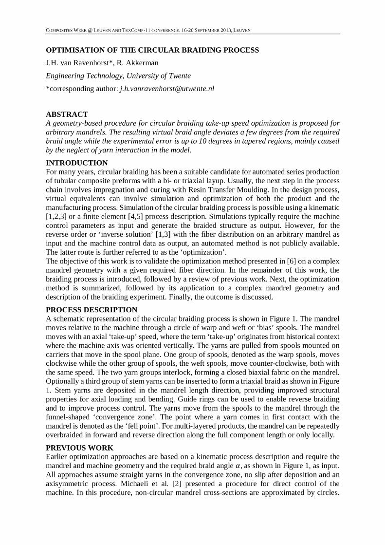
PROCESS DESCRIPTION A schematic representation of the circular braiding process is shown in Figure 1. The mandrel moves relative to the machine through a circle of warp and weft or ‘bias’ spools. The mandrel moves with an axial ‘take-up’ speed, where the term ‘take-up’ originates from historical context where the machine axis was oriented vertically. The yarns are pulled from spools mounted on carriers that move in the spool plane. One group of spools, denoted as the warp spools, moves clockwise while the other group of spools, the weft spools, move counter-clockwise, both with the same speed. The two yarn groups interlock, forming a closed biaxial fabric on the mandrel. Optionally a third group of stem yarns can be inserted to form a triaxial braid as shown in Figure 1. Stem yarns are deposited in the mandrel length direction, providing improved structural properties for axial loading and bending. Guide rings can be used to enable reverse braiding and to improve process control. The yarns move from the spools to the mandrel through the funnel-shaped ‘convergence zone’. The point where a yarn comes in first contact with the mandrel is denoted as the ‘fell point’. For multi-layered products, the mandrel can be repeatedly overbraided in forward and reverse direction along the full component length or only locally.

PREVIOUS WORK Earlier optimization approaches are based on a kinematic process description and require the mandrel and machine geometry and the required braid angle 훼, as shown in Figure 1, as input. All approaches assume straight yarns in the convergence zone, no slip after deposition and an axisymmetric process. Michaeli et al. [2] presented a procedure for direct control of the machine. In this procedure, non-circular mandrel cross-sections are approximated by circles.


The carrier speed must be provided as input and the take-up speed is output as a function of time. Du and Popper [3] optimized either the carrier speed or the take-up speed, depending on the user's choice, while keeping the other speed constant. The mandrel geometry is restricted to be rotation symmetric and is approximated by a series of conical segments.

Figure 1. Schematic representation of a circular braiding machine and a triaxial braid, showing braid angle 훼.

MATHEMATICAL MODEL The braid angle optimization procedure makes use of a kinematic simulation model that is described first. Next, the optimization model is introduced. In this work, a process ‘simulation’ denotes the conversion of given speeds to braid angle and a process ‘optimization’ denotes the inverse, i.e. conversion from a given braid angle to the take-up speed.

SIMULATION MODEL For the process model used in the simulation, it is assumed that the trajectories of the deposited yarns are continuous, differentiable, lie on the mandrel surface and remain fixed after first contact. Furthermore, it is assumed that yarns do not interact with each other, no friction between yarns and guide rings occurs and the yarn thickness can be neglected. Based on these assumptions, each yarn can be modelled independently as shown in Figure 1. Input parameters, as far as required for the purpose of this work, are described next. The simulation uses a time-stepping method with a constant time step size Δ푡 and the carrier rotational speed 휔(푡) and take-up speed 푣(푡) given as input. The mandrel is represented by a triangulated surface S and arbitrary centerline L. S must be a single closed shell without holes or large protrusions and is defined in the global Cartesian mandrel coordinate system with unit axes {퐱, 퐲, 퐳}. The surface region to be overbraided is bounded by a planar start- and end contour on S. The machine orientation is represented using a local Cartesian machine coordinate system with origin 퐦, here assumed to be coincident with the centerline, and unit axes {퐮, 퐯,퐰} which moves as a function of time with 퐰 assumed tangent to the centerline. The machine is parameterized with the machine spool plane circle radius 푟 and the optional inner and outer guide ring radii 푟 , and 푟 , and heights ℎ , and ℎ , . The number of yarns per yarn group is given by 푛 . Assuming 휔(푡) constant, the spool trajectory for the 푖-th spool of a bias yarn group is approximated with a helix-like curve Q around the centerline. 휑 is the spool plane angle and the spools are distributed evenly over the spool plane circle. Define the ‘supply point’ position vector 퐬 as the point from which a yarn is supplied, obtained by

퐬 = 퐪, ifnoguideringcontact,퐫, ifguideringcontact. (1)


Define the ‘creating circle’ as the circle that contains 퐬. The ‘free segment’ is defined as the yarn from 퐩 to 퐬. Depending on the input parameters, 퐬 may alternate between the spool plane circle and guide ring circles. The resulting supply point trajectory of퐬 is denoted by T. For a centered cylindrical mandrel, the braid angle is expressed using the ‘classical solution’ [7]

훼 = arctan휔푟푣 (2)

where 푟 is the mandrel radius. This relation is sometimes [1] generalized for mandrels with an arbitrary cross-section using

푟 =푝2휋 (3)

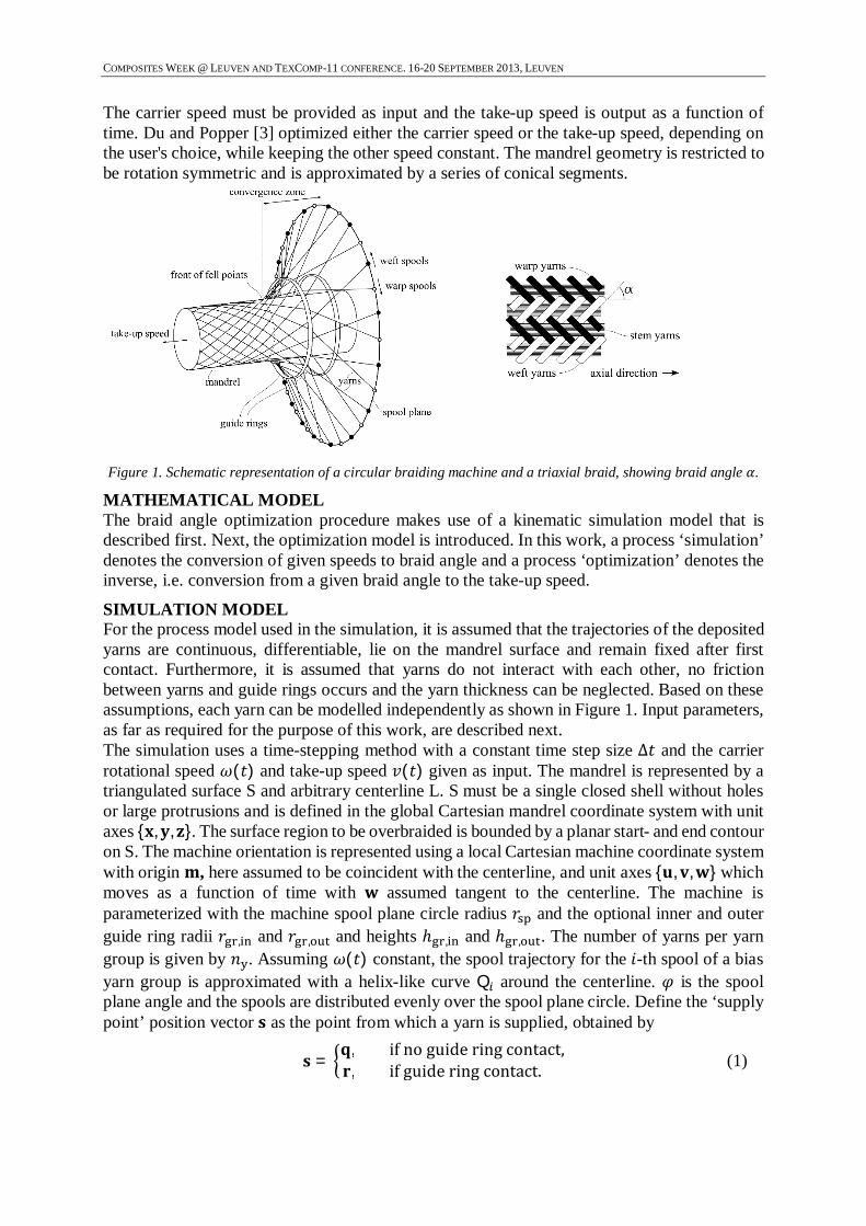
where 푝 is the mandrel cross-sectional perimeter. For arbitrary shapes, a deposition model similar to [8] is used where contact between the free segment and element edges in the neighborhood of the fell point is checked at each time step. The interlacement of the resulting deposited bias yarns provides geometrical bounds that form ‘tunnels’ through the biaxial braid for optional stem yarns. The centerline of each tunnel forms a stem yarn trajectory as described in [9]. As a result, the simulation outputs the yarn trajectories Y, and, implicitly, convergence zone length 퐻 as a function of, among others, the spool trajectories Q.

Figure 2. Process model for a single yarn, showing only the outer guide ring for clarity.

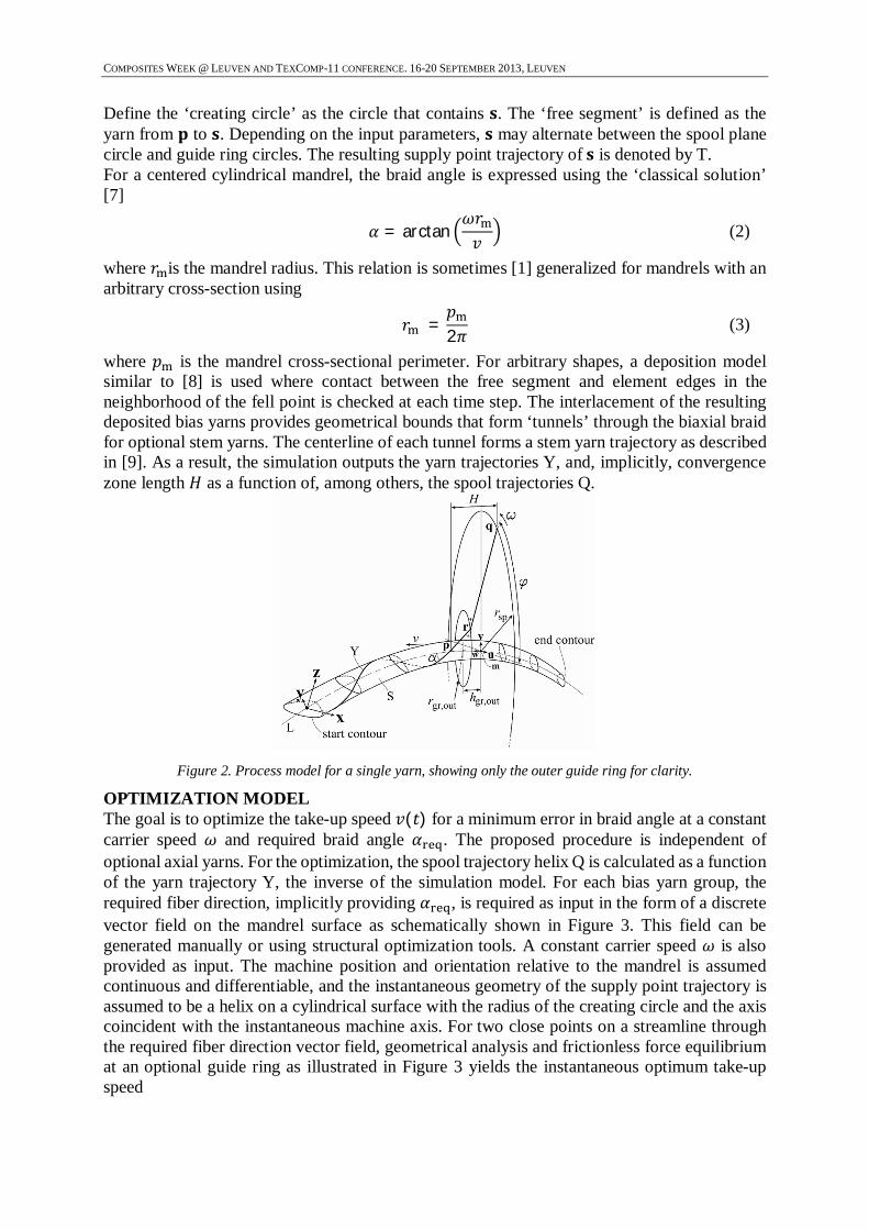
OPTIMIZATION MODEL The goal is to optimize the take-up speed 푣(푡) for a minimum error in braid angle at a constant carrier speed 휔 and required braid angle 훼 . The proposed procedure is independent of optional axial yarns. For the optimization, the spool trajectory helix Q is calculated as a function of the yarn trajectory Y, the inverse of the simulation model. For each bias yarn group, the required fiber direction, implicitly providing 훼 , is required as input in the form of a discrete vector field on the mandrel surface as schematically shown in Figure 3. This field can be generated manually or using structural optimization tools. A constant carrier speed 휔 is also provided as input. The machine position and orientation relative to the mandrel is assumed continuous and differentiable, and the instantaneous geometry of the supply point trajectory is assumed to be a helix on a cylindrical surface with the radius of the creating circle and the axis coincident with the instantaneous machine axis. For two close points on a streamline through the required fiber direction vector field, geometrical analysis and frictionless force equilibrium at an optional guide ring as illustrated in Figure 3 yields the instantaneous optimum take-up speed


푣 = 휔Δ푧Δ휑 (4)

for a single bias yarn. For all bias yarns, a weighted average of the individual optimal take-up speeds is used to generate the optimum process take-up speed. At point a, either the instantaneous streamline tangent can be used, or the actual deposited fiber tangent to form ‘feed-back’ for a more aggressive optimization yielding a faster response. The weight factor can be changed by optionally choosing a dominant ‘master’ mandrel side. The optimization procedure can also be used to determine the optimal start position of the mandrel relative to the machine. For details, see [6]. Note that yarn interaction, including friction, is not taken into account, likely leading to a significant systematic error that is not treated in this work.

Figure 3. Geometry for the optimum take-up speed calculation. Points 풂 and 풃 result in points 풂′ and 풃′,

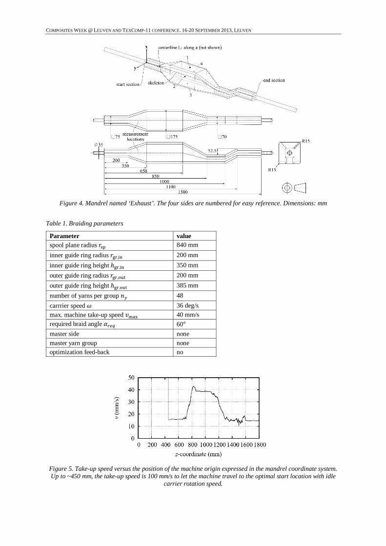
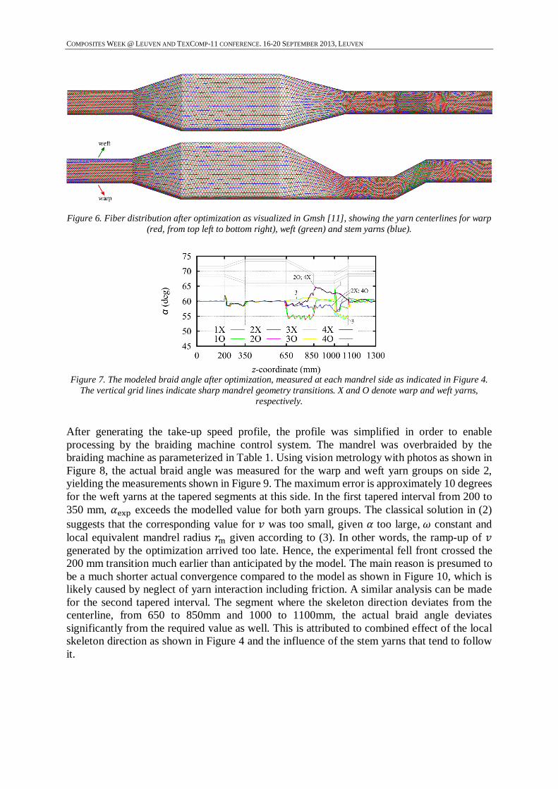
respectively, in turn providing the instantaneous spool helix. EXPERIMENT The experimental validation of the optimization procedure was performed at Eurocarbon, using the mandrel from Figure 4 as used in earlier research [1, 10], and the parameters from Table 1. Stem yarns are included, yielding a triaxial braid with a ‘regular’ or 2/2-twill interlacement type for the bias yarns. The required bias braid angle of 60° is used to obtain a quasi-isotropic layup. No master side was specified, allowing each mandrel side to participate equally in the optimization. The optimization generated the take-up speed profile in Figure 5. The values are close to those when calculated by the classical solution (2) and (3). Although the take-up speed is calculated as the average of all bias yarns, it still contains noise which is affected, amongst others, by the mesh ‘roughness’ and the chosen optimization arc length on the fiber streamline, shown in Figure 3 as the distance on the mandrel surface from 퐚 to 퐛. Note the counter-intuitive overshoot at 800mm, exceeding 40 mm/s. Figure 6 shows the resulting fiber distribution, including stem yarns that are deposited as a function of the deposited bias yarns. The resulting virtual braid angle is plotted in Figure 7, showing a maximum error of approximately 10 degrees for this optimized model.


Figure 4. Mandrel named ‘Exhaust’. The four sides are numbered for easy reference. Dimensions: mm

Table 1. Braiding parameters

Parameter value spool plane radius 푟 840 mm inner guide ring radius 푟 , 200 mm inner guide ring height ℎ , 350 mm outer guide ring radius 푟 , 200 mm outer guide ring height ℎ , 385 mm number of yarns per group 푛 48 carrrier speed 휔 36 deg/s max. machine take-up speed 푣 40 mm/s required braid angle 훼 60° master side none master yarn group none optimization feed-back no

Figure 5. Take-up speed versus the position of the machine origin expressed in the mandrel coordinate system. Up to ~450 mm, the take-up speed is 100 mm/s to let the machine travel to the optimal start location with idle

carrier rotation speed.


Figure 6. Fiber distribution after optimization as visualized in Gmsh [11], showing the yarn centerlines for warp

(red, from top left to bottom right), weft (green) and stem yarns (blue).

Figure 7. The modeled braid angle after optimization, measured at each mandrel side as indicated in Figure 4.

The vertical grid lines indicate sharp mandrel geometry transitions. X and O denote warp and weft yarns, respectively.

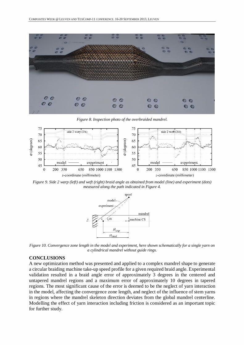
After generating the take-up speed profile, the profile was simplified in order to enable processing by the braiding machine control system. The mandrel was overbraided by the braiding machine as parameterized in Table 1. Using vision metrology with photos as shown in Figure 8, the actual braid angle was measured for the warp and weft yarn groups on side 2, yielding the measurements shown in Figure 9. The maximum error is approximately 10 degrees for the weft yarns at the tapered segments at this side. In the first tapered interval from 200 to 350 mm, 훼 exceeds the modelled value for both yarn groups. The classical solution in (2) suggests that the corresponding value for 푣 was too small, given 훼 too large,휔 constant and local equivalent mandrel radius 푟 given according to (3). In other words, the ramp-up of 푣 generated by the optimization arrived too late. Hence, the experimental fell front crossed the 200 mm transition much earlier than anticipated by the model. The main reason is presumed to be a much shorter actual convergence compared to the model as shown in Figure 10, which is likely caused by neglect of yarn interaction including friction. A similar analysis can be made for the second tapered interval. The segment where the skeleton direction deviates from the centerline, from 650 to 850mm and 1000 to 1100mm, the actual braid angle deviates significantly from the required value as well. This is attributed to combined effect of the local skeleton direction as shown in Figure 4 and the influence of the stem yarns that tend to follow it.


Figure 8. Inspection photo of the overbraided mandrel.

Figure 9. Side 2 warp (left) and weft (right) braid angle as obtained from model (line) and experiment (dots)

measured along the path indicated in Figure 4.

Figure 10. Convergence zone length in the model and experiment, here shown schematically for a single yarn on

a cylindrical mandrel without guide rings.

CONCLUSIONS A new optimization method was presented and applied to a complex mandrel shape to generate a circular braiding machine take-up speed profile for a given required braid angle. Experimental validation resulted in a braid angle error of approximately 3 degrees in the centered and untapered mandrel regions and a maximum error of approximately 10 degrees in tapered regions. The most significant cause of the error is deemed to be the neglect of yarn interaction in the model, affecting the convergence zone length, and neglect of the influence of stem yarns in regions where the mandrel skeleton direction deviates from the global mandrel centerline. Modelling the effect of yarn interaction including friction is considered as an important topic for further study.


ACKNOWLEDGEMENTS The support of Agentschap NL, Eurocarbon B.V. and the Dutch National Aerospace Laboratory NLR is gratefully acknowledged.

REFERENCES [1] Kessels, J. and Akkerman, R. Prediction of the yarn trajectories on complex braided preforms, Composites

Part A, Vol. 33, No. 8, pp 1073-1081, 2002 [2] Michaeli, W., Rosenbaum, U. and Jehrke, M. Processing strategy for braiding of complex-shaped parts

based on a mathematical process description, Composites Manufacturing, Vol. 1, No. 4, pp 243-251, 1990 [3] Du, G. and Popper, P. Analysis of a Circular Braiding Process for Complex Shapes, Journal of the textile

institute, Vol. 85, No. 3, pp 316-337, 1994 [4] Pickett, A., Sirtautas, J. and Erber, A. Braiding Simulation and Prediction of Mechanical Properties, Applied

Composite Materials, Vol. 16, No. 6, pp 345-364, 2009 [5] Stueve, J. and Gries, T. Advances in the simulation of the overbraiding process using FEM, COMPOSITES

- Innovative Materials for smarter Solutions, SEICO 09 ; SAMPE Europe 30th international jubilee conference and forum, pp 618-625, 2009

[6] Akkerman, R. and van Ravenhorst, J.H. Braid angle optimization for circular braiding, Composites Part A (under review), 2013

[7] Ko, F.K. Engineered materials handbook, ASM International, 1987 [8] Akkerman, R. and Villa Rodriguez, B.H. Braiding simulation for RTM preforms, Proceedings of

TEXCOMP-8, 2006 [9] Akkerman, R. and van Ravenhorst, J.H. A spool pattern tool for circular braiding, ICCM18 conference

proceedings, ICCM18, 2011 [10] Nishimoto, H., Ohtani, A., Nakai, A. and Hamada, H. Prediction Method for Temporal Change in Fiber

Orientation on Cylindrical Braided Preforms, Textile Research Journal, Vol. 80, No. 9, pp 814-821, 2010 [11] Geuzaine, C., Remacle, J.-F. Gmsh: a three-dimensional finite element mesh generator with built-in pre- and

post-processing facilities, International Journal for Numerical Methods in Engineering, Vol. 79, No. 11, pp 1309-1331, 2009

Documents

OPTIMISATION OF THE CIRCULAR BRAIDING PROCESS · OPTIMISATION OF THE CIRCULAR BRAIDING ... Simulation of the circular braiding process is possible using ... the spool trajectory for