Embed Size (px)
Citation preview

Optimization in ComPASS-4
Stefan Wild & Jeff Larson
Argonne National LaboratoryMathematics and Computer Science Division
April 23, 2018
The Plan
1. Optimization Formulations and Taxonomy Stochastic Optimization Multiobjective Optimization Simulation-Based Optimization Derivative-Free Optimization Global Optimization
2. An Example LPA Optimization to Highlight Challenges
3. POPAS
4. Why not Blackbox Optimization
5. APOSMM
ComPASS-4, April 2018 1
Mathematical/Numerical Nonlinear Optimization
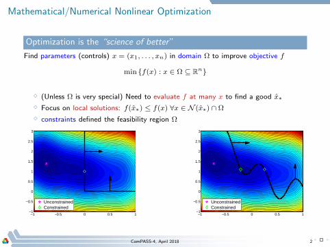
Optimization is the “science of better”
Find parameters (controls) x = (x1, . . . , xn) in domain Ω to improve objective f
min f(x) : x ∈ Ω ⊆ Rn
⋄ (Unless Ω is very special) Need to evaluate f at many x to find a good x∗⋄ Focus on local solutions: f(x∗) ≤ f(x) ∀x ∈ N (x∗) ∩ Ω
⋄ constraints defined the feasibility region Ω
−1 −0.5 0 0.5 1−1
−0.5
0
0.5
1
1.5
2
2.5
3
UnconstrainedConstrained
−1 −0.5 0 0.5 1−1
−0.5
0
0.5
1
1.5
2
2.5
3
UnconstrainedConstrained
ComPASS-4, April 2018 2
Stochastic Optimization
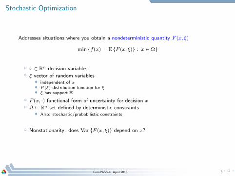
Addresses situations where you obtain a nondeterministic quantity F (x, ξ)
min f(x) = E F (x, ξ) : x ∈ Ω
⋄ x ∈ Rn decision variables
⋄ ξ vector of random variables independent of x P (ξ) distribution function for ξ ξ has support Ξ
⋄ F (x, ·) functional form of uncertainty for decision x
⋄ Ω ⊆ Rn set defined by deterministic constraints
Also: stochastic/probabilistic constraints
⋄ Nonstationarity: does Var F (x, ξ) depend on x?
ComPASS-4, April 2018 3
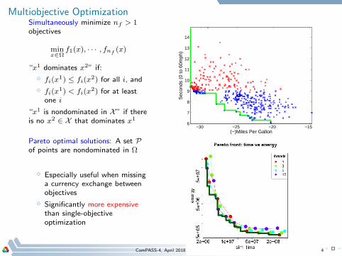
Multiobjective OptimizationSimultaneously minimize nf > 1objectives
minx∈Ω
f1(x), · · · , fnf(x)
“x1 dominates x2” if:
⋄ fi(x1) ≤ fi(x
2) for all i, and
⋄ fi(x1) < fi(x
2) for at leastone i
“x1 is nondominated in X” if thereis no x2 ∈ X that dominates x1
Pareto optimal solutions: A set Pof points are nondominated in Ω
⋄ Especially useful when missinga currency exchange betweenobjectives
⋄ Significantly more expensivethan single-objectiveoptimization
−30 −25 −20 −156
7
8
9
10
11
12
13
14
Sec
onds
(0
to 6
0mph
)
(−)Miles Per Gallon
ComPASS-4, April 2018 4
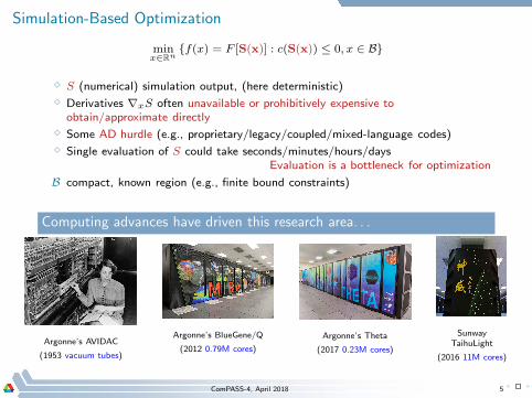
Simulation-Based Optimization
minx∈Rn
f(x) = F [S(x)] : c(S(x)) ≤ 0, x ∈ B
⋄ S (numerical) simulation output, (here deterministic)
⋄ Derivatives ∇xS often unavailable or prohibitively expensive toobtain/approximate directly
⋄ Some AD hurdle (e.g., proprietary/legacy/coupled/mixed-language codes)
⋄ Single evaluation of S could take seconds/minutes/hours/daysEvaluation is a bottleneck for optimization
B compact, known region (e.g., finite bound constraints)
Computing advances have driven this research area. . .
Argonne’s AVIDAC
(1953 vacuum tubes)
Argonne’s BlueGene/Q
(2012 0.79M cores)
Argonne’s Theta
(2017 0.23M cores)
SunwayTaihuLight
(2016 11M cores)
ComPASS-4, April 2018 5
Derivative-Free/Zero-Order Optimization
“Some derivatives are unavailable for optimization purposes”
ComPASS-4, April 2018 6
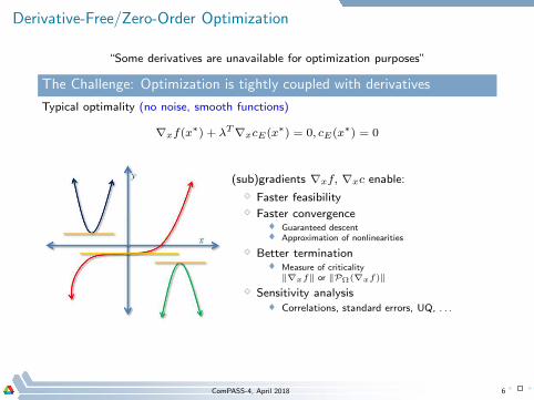
Derivative-Free/Zero-Order Optimization
“Some derivatives are unavailable for optimization purposes”
The Challenge: Optimization is tightly coupled with derivatives
Typical optimality (no noise, smooth functions)
∇xf(x∗) + λT∇xcE(x∗) = 0, cE(x∗) = 0
(sub)gradients ∇xf, ∇xc enable:
⋄ Faster feasibility⋄ Faster convergence
Guaranteed descent Approximation of nonlinearities
⋄ Better termination Measure of criticality
‖∇xf‖ or ‖PΩ(∇xf)‖⋄ Sensitivity analysis
Correlations, standard errors, UQ, . . .
ComPASS-4, April 2018 6
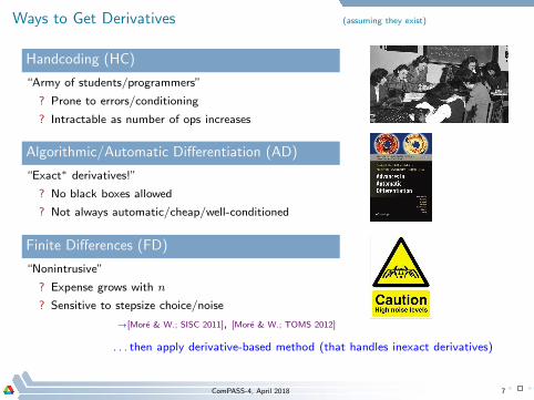
Ways to Get Derivatives (assuming they exist)
Handcoding (HC)
“Army of students/programmers”
? Prone to errors/conditioning
? Intractable as number of ops increases
Algorithmic/Automatic Differentiation (AD)
“Exact∗ derivatives!”
? No black boxes allowed
? Not always automatic/cheap/well-conditioned
Finite Differences (FD)
“Nonintrusive”
? Expense grows with n
? Sensitive to stepsize choice/noise
→[More & W.; SISC 2011], [More & W.; TOMS 2012]
. . . then apply derivative-based method (that handles inexact derivatives)
ComPASS-4, April 2018 7
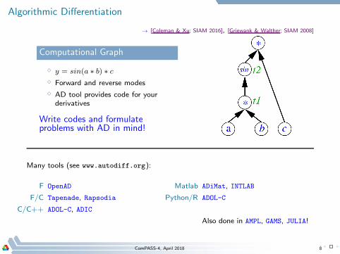
Algorithmic Differentiation
→ [Coleman & Xu; SIAM 2016], [Griewank & Walther; SIAM 2008]
Computational Graph
⋄ y = sin(a ∗ b) ∗ c
⋄ Forward and reverse modes
⋄ AD tool provides code for yourderivatives
Write codes and formulateproblems with AD in mind!
Many tools (see www.autodiff.org):
F OpenAD
F/C Tapenade, Rapsodia
C/C++ ADOL-C, ADIC
Matlab ADiMat, INTLAB
Python/R ADOL-C
Also done in AMPL, GAMS, JULIA!
ComPASS-4, April 2018 8
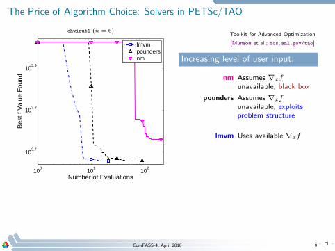
The Price of Algorithm Choice: Solvers in PETSc/TAO
chwirut1 (n = 6)
100
101
102
103.7
103.8
103.9
Number of Evaluations
Bes
t f V
alue
Fou
nd
lmvmpoundersnm
Toolkit for Advanced Optimization
[Munson et al.; mcs.anl.gov/tao]
Increasing level of user input:
nm Assumes ∇xf
unavailable, black box
pounders Assumes ∇xf
unavailable, exploitsproblem structure
lmvm Uses available ∇xf
ComPASS-4, April 2018 9
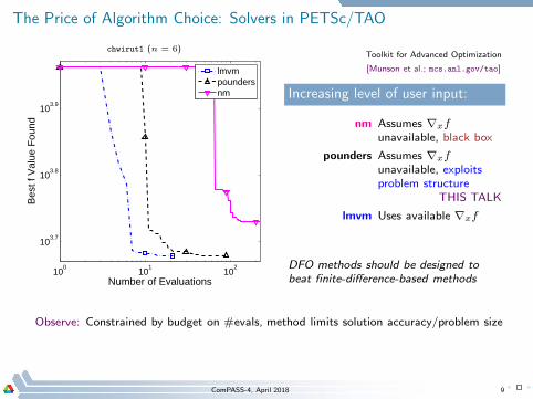
The Price of Algorithm Choice: Solvers in PETSc/TAO
chwirut1 (n = 6)
100
101
102
103.7
103.8
103.9
Number of Evaluations
Bes
t f V
alue
Fou
nd
lmvmpoundersnm
Toolkit for Advanced Optimization
[Munson et al.; mcs.anl.gov/tao]
Increasing level of user input:
nm Assumes ∇xf
unavailable, black box
pounders Assumes ∇xf
unavailable, exploitsproblem structure
THIS TALK
lmvm Uses available ∇xf
DFO methods should be designed to
beat finite-difference-based methods
Observe: Constrained by budget on #evals, method limits solution accuracy/problem size
ComPASS-4, April 2018 9
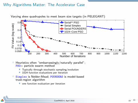
Why Algorithms Matter: The Accelerator Case
Varying skew quadrupoles to meet beam size targets (in PELEGANT)
100 200 300 400 500 600 700 800 900 1000 1100 12000.0580.075
0.1
0.14
0.2
0.4
0.8
Number of Iterations
Fit
Val
ue (
log
scal
e)
Serial** PSOSerial SimplexSerial POUNDERS1024−Core PSO
⋄ Heuristics often “embarrassingly/naturally parallel”;PSO= particle swarm method
Typically through stochastic sampling/evolution 1024 function evaluations per iteration
⋄ Simplex is Nelder-Mead; POUNDERS is model-basedtrust-region algorithm
one function evaluation per iteration
ComPASS-4, April 2018 10
Global Optimization, minx∈Ω f(x)
Careful:
⋄ Global convergence: Convergence (to a local solution/stationary point) fromanywhere in Ω
⋄ Convergence to a global minimizer: Obtain x∗ with f(x∗) ≤ f(x)∀x ∈ Ω
ComPASS-4, April 2018 11
Global Optimization, minx∈Ω f(x)
Careful:
⋄ Global convergence: Convergence (to a local solution/stationary point) fromanywhere in Ω
⋄ Convergence to a global minimizer: Obtain x∗ with f(x∗) ≤ f(x)∀x ∈ Ω
Anyone selling you global solutions when derivatives are unavailable:
either assumes more about your problem (e.g., convex f)
or expects you to wait forever
Torn and Zilinskas: An algorithm converges to the global minimum for anycontinuous f if and only if the sequence of points visited by thealgorithm is dense in Ω.
or cannot be trusted
Instead:
⋄ Rapidly find good local solutions and/or be robust to poor solutions
⋄ Consider multistart approaches and/or structure of multimodality
ComPASS-4, April 2018 11
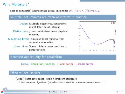
Why Multistart?
Best minimizer(s) approximate global minimizer x∗, f(x∗) ≤ f(x)∀x ∈ D
Multiple local minima are often of interest in practice
Design Multiple objectives/constraintsmight later be of interest
Distinctness j best minimizers have physicalmeaning
Simulation Errors Spurious local minima fromsimulator anomalies
Uncertainty Some minima more sensitive toperturbations 1 1.5 2 2.5 3 3.5 4 4.5 5 5.5 6
−3.5
−3
−2.5
−2
−1.5
−1
−0.5
0
0.5
Min AMinB
Increased opportunity for parallelism
Trilevel simulation/function → local solver → global solver
Efficient local solvers
⋄ (Local) surrogate-based, exploit problem structure least-squares objectives, (un)relaxable constraints, known nonsmoothness, . . .
ComPASS-4, April 2018 12
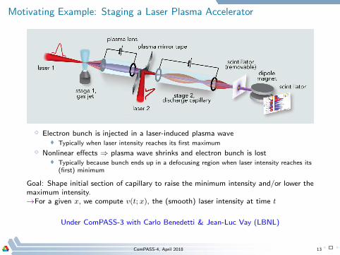
Motivating Example: Staging a Laser Plasma Accelerator
⋄ Electron bunch is injected in a laser-induced plasma wave Typically when laser intensity reaches its first maximum
⋄ Nonlinear effects ⇒ plasma wave shrinks and electron bunch is lost Typically because bunch ends up in a defocusing region when laser intensity reaches its
(first) minimum
Goal: Shape initial section of capillary to raise the minimum intensity and/or lower themaximum intensity.→For a given x, we compute v(t; x), the (smooth) laser intensity at time t
Under ComPASS-3 with Carlo Benedetti & Jean-Luc Vay (LBNL)
ComPASS-4, April 2018 13
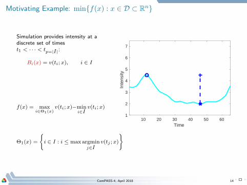
Motivating Example: minf(x) : x ∈ D ⊂ Rn
Simulation provides intensity at adiscrete set of timest1 < · · · < tp=|I|:
Bi(x) = v(ti; x), i ∈ I
f(x) = maxi∈Θ1(x)
v(ti;x)−mini∈I
v(ti;x)
Θ1(x) =
i ∈ I : i ≤ max argminj∈I
v(tj ; x)
10 20 30 40 50 60Time
1
2
3
4
5
6
7
Inte
nsity
ComPASS-4, April 2018 14
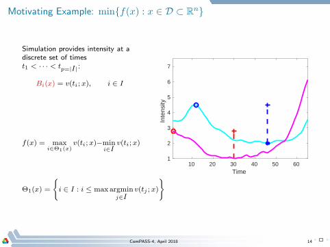
Motivating Example: minf(x) : x ∈ D ⊂ Rn
Simulation provides intensity at adiscrete set of timest1 < · · · < tp=|I|:
Bi(x) = v(ti; x), i ∈ I
f(x) = maxi∈Θ1(x)
v(ti;x)−mini∈I
v(ti;x)
Θ1(x) =
i ∈ I : i ≤ max argminj∈I
v(tj ; x)
10 20 30 40 50 60Time
1
2
3
4
5
6
7
Inte
nsity
ComPASS-4, April 2018 14
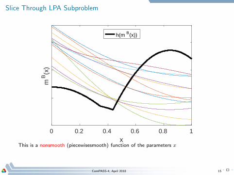
Slice Through LPA Subproblem
0 0.2 0.4 0.6 0.8 1x
mB(x
)
h(m B(x))
This is a nonsmooth (piecewisesmooth) function of the parameters x
ComPASS-4, April 2018 15
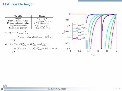
LPA Feasible Region
Variable RangeLength 2 ≤ L ≤ 6
Plasma channel radius 1 ≤ Xmax ≤ 1.5Minimum channel radius 0.7 ≤ Xmin ≤ 1Longitudinal location 0 ≤ Zmin ≤ 1Laser focus position −1.2 ≤ Zf ≤ 0
c1(x) = − XmaxZ4min
− (Xmax − Xmin)(2Zmin − 3Z2min)
≤0
c2(x) =Xmax(Z4min − 4Z
3min + 3Z
2min)
+ (Xmax − Xmin)(3Z2min − 4Zmin + 1)
≤0 0 0.2 0.4 0.6 0.8 1Z
min
0.7
0.75
0.8
0.85
0.9
0.95
1
Xm
in
Xmax
=1
Xmax
=1.01
Xmax
=1.1
Xmax
=1.25
Xmax
=1.5
ComPASS-4, April 2018 16
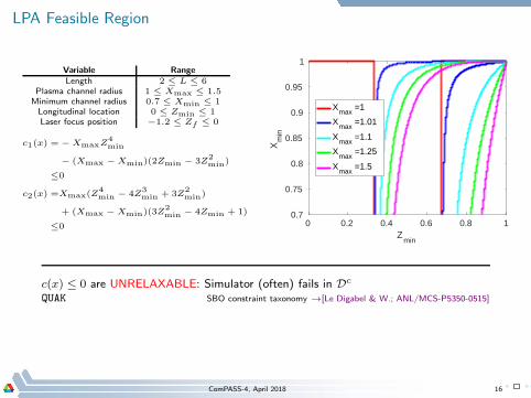
LPA Feasible Region
Variable RangeLength 2 ≤ L ≤ 6
Plasma channel radius 1 ≤ Xmax ≤ 1.5Minimum channel radius 0.7 ≤ Xmin ≤ 1Longitudinal location 0 ≤ Zmin ≤ 1Laser focus position −1.2 ≤ Zf ≤ 0
c1(x) = − XmaxZ4min
− (Xmax − Xmin)(2Zmin − 3Z2min)
≤0
c2(x) =Xmax(Z4min − 4Z
3min + 3Z
2min)
+ (Xmax − Xmin)(3Z2min − 4Zmin + 1)
≤0 0 0.2 0.4 0.6 0.8 1Z
min
0.7
0.75
0.8
0.85
0.9
0.95
1
Xm
in
Xmax
=1
Xmax
=1.01
Xmax
=1.1
Xmax
=1.25
Xmax
=1.5
c(x) ≤ 0 are UNRELAXABLE: Simulator (often) fails in Dc
QUAK SBO constraint taxonomy →[Le Digabel & W.; ANL/MCS-P5350-0515]
ComPASS-4, April 2018 16
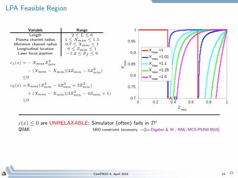
LPA Feasible Region
Variable RangeLength 2 ≤ L ≤ 6
Plasma channel radius 1 ≤ Xmax ≤ 1.5Minimum channel radius 0.7 ≤ Xmin ≤ 1Longitudinal location 0 ≤ Zmin ≤ 1Laser focus position −1.2 ≤ Zf ≤ 0
c1(x) = − XmaxZ4min
− (Xmax − Xmin)(2Zmin − 3Z2min)
≤0
c2(x) =Xmax(Z4min − 4Z
3min + 3Z
2min)
+ (Xmax − Xmin)(3Z2min − 4Zmin + 1)
≤0 0 0.2 0.4 0.6 0.8 1Z
min
0.7
0.75
0.8
0.85
0.9
0.95
1
Xm
in
A B
Xmax
=1
Xmax
=1.01
Xmax
=1.1
Xmax
=1.25
Xmax
=1.5
c(x) ≤ 0 are UNRELAXABLE: Simulator (often) fails in Dc
QUAK SBO constraint taxonomy →[Le Digabel & W.; ANL/MCS-P5350-0515]
ComPASS-4, April 2018 16
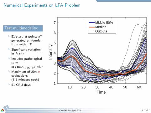
Numerical Experiments on LPA Problem
Test multimodality:
⋄ 51 starting points x0
generated uniformlyfrom within D
⋄ Significant variationin f(x0)
⋄ Includes pathologicalt1 =argmaxi∈Θ1(x0) v(ti;x
0)
⋄ Maximum of 20n v
evaluations(7.5 minutes each)
⋄ 51 CPU days10 20 30 40 50 60
Time
1
2
3
4
5
6
7
Inte
nsity
Middle 50%MedianOutputs
ComPASS-4, April 2018 17
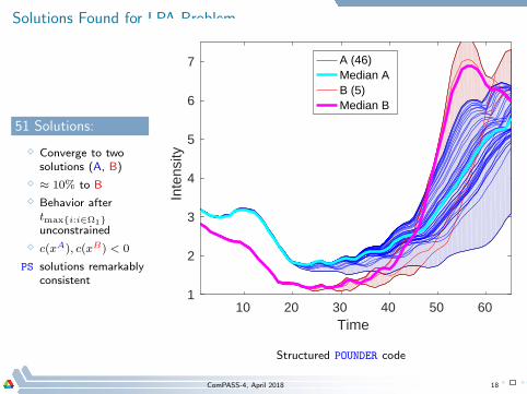
Solutions Found for LPA Problem
51 Solutions:
⋄ Converge to twosolutions (A, B)
⋄ ≈ 10% to B
⋄ Behavior aftertmaxi:i∈Ω1unconstrained
⋄ c(xA), c(xB) < 0
PS solutions remarkablyconsistent
10 20 30 40 50 60Time
1
2
3
4
5
6
7
Inte
nsity
A (46)Median AB (5)Median B
Structured POUNDER code
ComPASS-4, April 2018 18
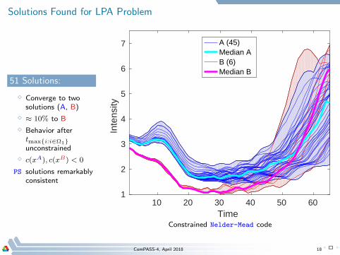
Solutions Found for LPA Problem
51 Solutions:
⋄ Converge to twosolutions (A, B)
⋄ ≈ 10% to B
⋄ Behavior aftertmaxi:i∈Ω1unconstrained
⋄ c(xA), c(xB) < 0
PS solutions remarkablyconsistent
10 20 30 40 50 60Time
1
2
3
4
5
6
7
Inte
nsity
A (45)Median AB (6)Median B
Constrained Nelder-Mead code
ComPASS-4, April 2018 18
POPAS Activity Proposed for ComPASS-4
Platform for Optimization of Particle Accelerators at Scale
⋄ integrated platform for coordinating the evaluation and numerical optimization ofaccelerator simulations on leadership-class DOE computers
⋄ orchestrate concurrent evaluations of OSIRIS, QuickPIC, Synergia, and MARS (orcombinations thereof) with distinct inputs/parameter values
⋄ account for resource requirements of the above
⋄ API will allow the user to describe the mapping from simulation outputs and thederived quantities of interest used to define objective and constraint quantities
TH: Provide enough information so that optimization is efficient
ComPASS-4, April 2018 19
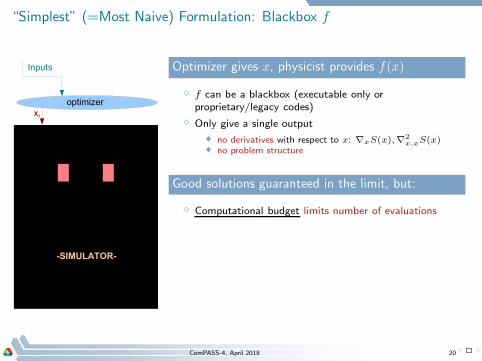
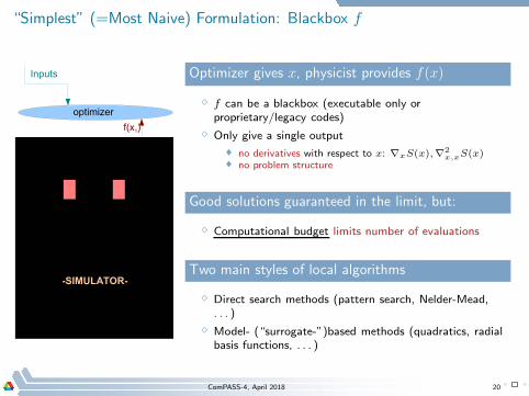
“Simplest” (=Most Naive) Formulation: Blackbox f
Optimizer gives x, physicist provides f(x)
⋄ f can be a blackbox (executable only orproprietary/legacy codes)
⋄ Only give a single output
no derivatives with respect to x: ∇xS(x),∇2x,xS(x)
no problem structure
Good solutions guaranteed in the limit, but:
⋄ Computational budget limits number of evaluations
ComPASS-4, April 2018 20
“Simplest” (=Most Naive) Formulation: Blackbox f
Optimizer gives x, physicist provides f(x)
⋄ f can be a blackbox (executable only orproprietary/legacy codes)
⋄ Only give a single output
no derivatives with respect to x: ∇xS(x),∇2x,xS(x)
no problem structure
Good solutions guaranteed in the limit, but:
⋄ Computational budget limits number of evaluations
Two main styles of local algorithms
⋄ Direct search methods (pattern search, Nelder-Mead,. . . )
⋄ Model- (“surrogate-”)based methods (quadratics, radialbasis functions, . . . )
ComPASS-4, April 2018 20
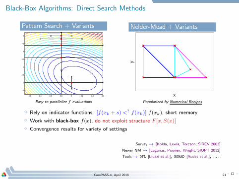
Black-Box Algorithms: Direct Search Methods
Pattern Search + Variants
2.2 2.4 2.6 2.8 3 3.2 3.4 3.6
1.5
2
2.5
3
3.5
4
4.5
5
Easy to parallelize f evaluations
Nelder-Mead + Variants
x
y
Popularized by Numerical Recipes
⋄ Rely on indicator functions: [f(xk + s) <? f(xk)] f(xk), short memory
⋄ Work with black-box f(x), do not exploit structure F [x,S(x)]
⋄ Convergence results for variety of settings
Survey → [Kolda, Lewis, Torczon; SIREV 2003]
Newer NM → [Lagarias, Poonen, Wright; SIOPT 2012]
Tools → DFL [Liuzzi et al.], NOMAD [Audet et al.], . . .
ComPASS-4, April 2018 21
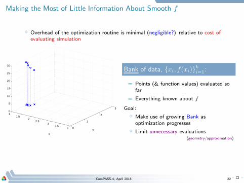
Making the Most of Little Information About Smooth f
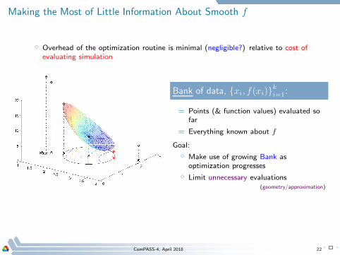
⋄ Overhead of the optimization routine is minimal (negligible?) relative to cost ofevaluating simulation
11.5
22.5
33.5
4 0
1
2
30
5
10
15
20
25
30
yx
Bank of data, xi, f(xi)k
i=1:
= Points (& function values) evaluated sofar
= Everything known about f
Goal:
⋄ Make use of growing Bank asoptimization progresses
⋄ Limit unnecessary evaluations(geometry/approximation)
ComPASS-4, April 2018 22
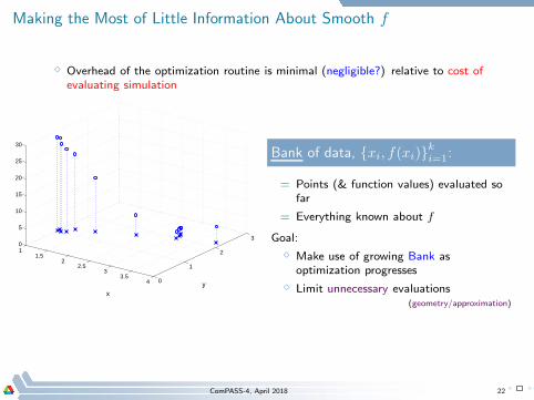
Making the Most of Little Information About Smooth f
⋄ Overhead of the optimization routine is minimal (negligible?) relative to cost ofevaluating simulation
11.5
22.5
33.5
4 0
1
2
30
5
10
15
20
25
30
yx
Bank of data, xi, f(xi)k
i=1:
= Points (& function values) evaluated sofar
= Everything known about f
Goal:
⋄ Make use of growing Bank asoptimization progresses
⋄ Limit unnecessary evaluations(geometry/approximation)
ComPASS-4, April 2018 22
Making the Most of Little Information About Smooth f
⋄ Overhead of the optimization routine is minimal (negligible?) relative to cost ofevaluating simulation
Bank of data, xi, f(xi)k
i=1:
= Points (& function values) evaluated sofar
= Everything known about f
Goal:
⋄ Make use of growing Bank asoptimization progresses
⋄ Limit unnecessary evaluations(geometry/approximation)
ComPASS-4, April 2018 22
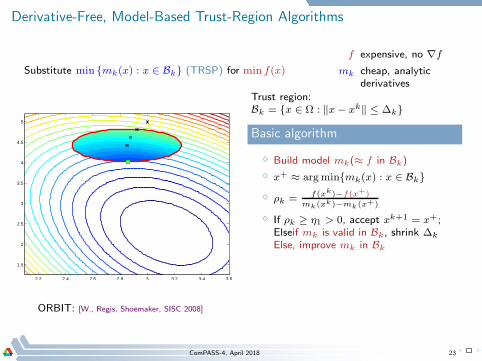
Derivative-Free, Model-Based Trust-Region Algorithms
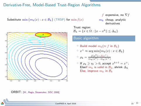
Substitute min mk(x) : x ∈ Bk (TRSP) for min f(x)
f expensive, no ∇f
mk cheap, analyticderivatives
2.2 2.4 2.6 2.8 3 3.2 3.4 3.6
1.5
2
2.5
3
3.5
4
4.5
5
Trust region:Bk = x ∈ Ω : ‖x− xk‖ ≤ ∆k
Basic algorithm
⋄ Build model mk(≈ f in Bk)
⋄ x+ ≈ argminmk(x) : x ∈ Bk
⋄ ρk =f(xk)−f(x+)
mk(xk)−mk(x+)
⋄ If ρk ≥ η1 > 0, accept xk+1 = x+;Elseif mk is valid in Bk, shrink ∆k
Else, improve mk in Bk
ORBIT: [W., Regis, Shoemaker, SISC 2008]
ComPASS-4, April 2018 23
Derivative-Free, Model-Based Trust-Region Algorithms
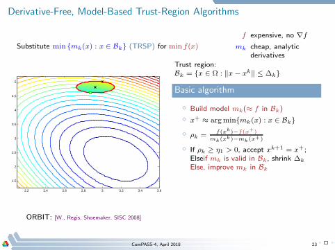
Substitute min mk(x) : x ∈ Bk (TRSP) for min f(x)
f expensive, no ∇f
mk cheap, analyticderivatives
2.2 2.4 2.6 2.8 3 3.2 3.4 3.6
1.5
2
2.5
3
3.5
4
4.5
5
Trust region:Bk = x ∈ Ω : ‖x− xk‖ ≤ ∆k
Basic algorithm
⋄ Build model mk(≈ f in Bk)
⋄ x+ ≈ argminmk(x) : x ∈ Bk
⋄ ρk =f(xk)−f(x+)
mk(xk)−mk(x+)
⋄ If ρk ≥ η1 > 0, accept xk+1 = x+;Elseif mk is valid in Bk, shrink ∆k
Else, improve mk in Bk
ORBIT: [W., Regis, Shoemaker, SISC 2008]
ComPASS-4, April 2018 23
Derivative-Free, Model-Based Trust-Region Algorithms
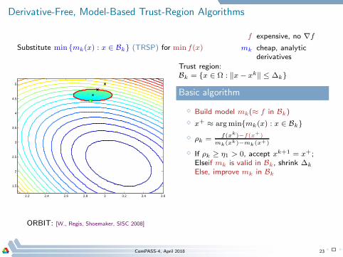
Substitute min mk(x) : x ∈ Bk (TRSP) for min f(x)
f expensive, no ∇f
mk cheap, analyticderivatives
2.2 2.4 2.6 2.8 3 3.2 3.4 3.6
1.5
2
2.5
3
3.5
4
4.5
5
Trust region:Bk = x ∈ Ω : ‖x− xk‖ ≤ ∆k
Basic algorithm
⋄ Build model mk(≈ f in Bk)
⋄ x+ ≈ argminmk(x) : x ∈ Bk
⋄ ρk =f(xk)−f(x+)
mk(xk)−mk(x+)
⋄ If ρk ≥ η1 > 0, accept xk+1 = x+;Elseif mk is valid in Bk, shrink ∆k
Else, improve mk in Bk
ORBIT: [W., Regis, Shoemaker, SISC 2008]
ComPASS-4, April 2018 23
Derivative-Free, Model-Based Trust-Region Algorithms
Substitute min mk(x) : x ∈ Bk (TRSP) for min f(x)
f expensive, no ∇f
mk cheap, analyticderivatives
2.2 2.4 2.6 2.8 3 3.2 3.4 3.6
1.5
2
2.5
3
3.5
4
4.5
5
Trust region:Bk = x ∈ Ω : ‖x− xk‖ ≤ ∆k
Basic algorithm
⋄ Build model mk(≈ f in Bk)
⋄ x+ ≈ argminmk(x) : x ∈ Bk
⋄ ρk = f(xk)−f(x+)
mk(xk)−mk(x+)
⋄ If ρk ≥ η1 > 0, accept xk+1 = x+;Elseif mk is valid in Bk, shrink ∆k
Else, improve mk in Bk
ORBIT: [W., Regis, Shoemaker, SISC 2008]
ComPASS-4, April 2018 23
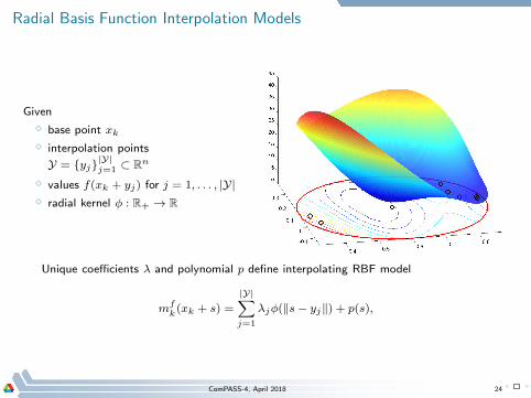
Radial Basis Function Interpolation Models
Given
⋄ base point xk
⋄ interpolation points
Y = yj|Y|j=1 ⊂ R
n
⋄ values f(xk + yj) for j = 1, . . . , |Y|
⋄ radial kernel φ : R+ → R
Unique coefficients λ and polynomial p define interpolating RBF model
mfk(xk + s) =
|Y|∑
j=1
λjφ(‖s− yj‖) + p(s),
ComPASS-4, April 2018 24
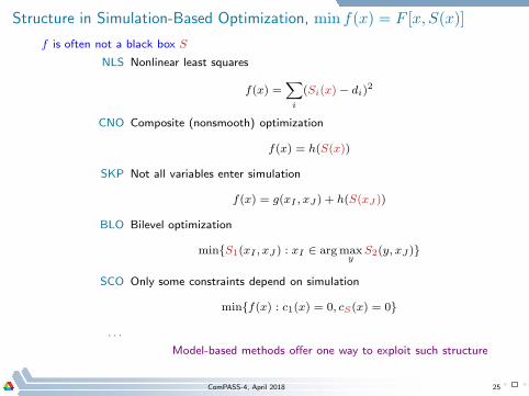
Structure in Simulation-Based Optimization, min f(x) = F [x, S(x)]
f is often not a black box S
NLS Nonlinear least squares
f(x) =∑
i
(Si(x)− di)2
CNO Composite (nonsmooth) optimization
f(x) = h(S(x))
SKP Not all variables enter simulation
f(x) = g(xI , xJ) + h(S(xJ ))
BLO Bilevel optimization
minS1(xI , xJ ) : xI ∈ argmaxy
S2(y, xJ)
SCO Only some constraints depend on simulation
minf(x) : c1(x) = 0, cS(x) = 0
. . .
Model-based methods offer one way to exploit such structure
ComPASS-4, April 2018 25
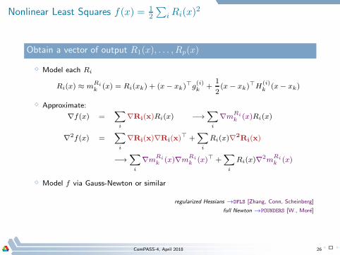
Nonlinear Least Squares f(x) = 12
∑iRi(x)
2
Obtain a vector of output R1(x), . . . , Rp(x)
⋄ Model each Ri
Ri(x) ≈ mRik
(x) = Ri(xk) + (x− xk)⊤g
(i)k
+1
2(x− xk)
⊤H(i)k
(x− xk)
⋄ Approximate:
∇f(x) =∑
i
∇Ri(x)Ri(x) −→∑
i
∇mRik (x)Ri(x)
∇2f(x) =∑
i
∇Ri(x)∇Ri(x)⊤ +
∑
i
Ri(x)∇2Ri(x)
−→∑
i
∇mRik (x)∇m
Rik (x)⊤ +
∑
i
Ri(x)∇2m
Rik (x)
⋄ Model f via Gauss-Newton or similar
regularized Hessians →DFLS [Zhang, Conn, Scheinberg]
full Newton →POUNDERS [W., More]
ComPASS-4, April 2018 26
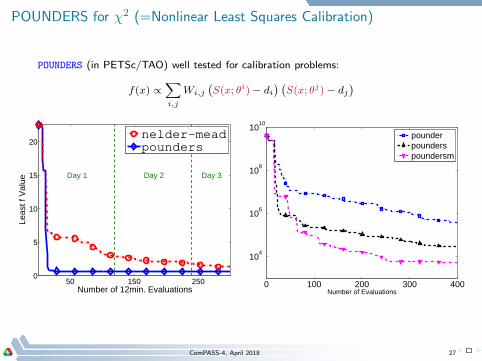
POUNDERS for χ2 (=Nonlinear Least Squares Calibration)
POUNDERS (in PETSc/TAO) well tested for calibration problems:
f(x) ∝∑
i,j
Wi,j
(
S(x; θi)− di) (
S(x; θj)− dj)
50 150 2500
5
10
15
20
Day 1 Day 2 Day 3
Number of 12min. Evaluations
Leas
t f V
alue
nelder−mead
pounders
0 100 200 300 400
104
106
108
1010
Number of Evaluations
pounderpounderspoundersm
ComPASS-4, April 2018 27
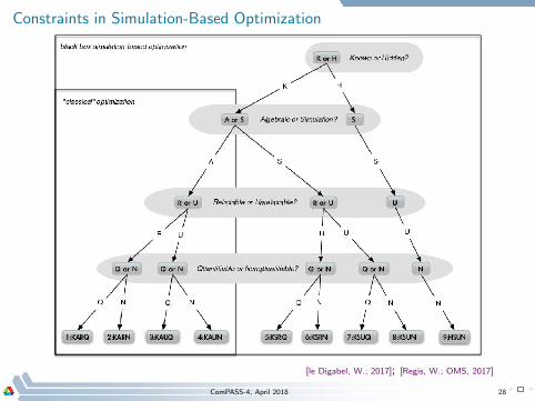
Constraints in Simulation-Based Optimization
[le Digabel, W.; 2017]; [Regis, W.; OMS, 2017]
ComPASS-4, April 2018 28
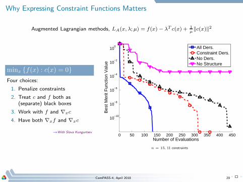
Why Expressing Constraint Functions Matters
Augmented Lagrangian methods, LA(x, λ;µ) = f(x) − λT c(x) + 1µ‖c(x)‖2
minx f(x) : c(x) = 0
Four choices:
1. Penalize constraints
2. Treat c and f both as(separate) black boxes
3. Work with f and ∇xc
4. Have both ∇xf and ∇xc
→With Slava Kungurtsev0 50 100 150 200 250 300 350 400 450
10−10
10−8
10−6
10−4
10−2
100
Number of Evaluations
Bes
t Mer
it F
unct
ion
Val
ue
All Ders.Constraint Ders.No Ders.No Structure
n = 15, 11 constraints
ComPASS-4, April 2018 29
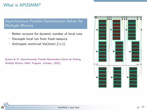
What is APOSMM?
Asynchronous Parallel Optimization Solver forMultiple Minima
⋄ Better account for dynamic number of local runs
⋄ Decouple local run from fixed resource
⋄ Anticipate nontrivial Var[time (f(x))]
[Larson & W. Asynchronously Parallel Optimization Solver for Finding
Multiple Minima, Math. Program. Comput., 2018.]
ComPASS-4, April 2018 30
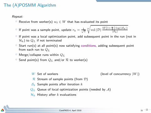
The (A)POSMM Algorithm
Repeat:
⋄ Receive from worker(s) wℓ ∈ W that has evaluated its point
⋄ If point was a sample point, update rk = 1√π
n
√
vol (D)5Γ(1+n
2 ) log(|Sk|)|Sk|
⋄ If point was a local optimization point, add subsequent point in the run (not inHk) to QL if not terminated
⋄ Start run(s) at all point(s) now satisfying conditions, adding subsequent pointfrom each run to QL
⋄ Merge/collapse runs within QL
⋄ Send point(s) from QL and/or R to worker(s)
W Set of workers (level of concurrency |W |)
R Stream of sample points (from D)
Sk Sample points after iteration k
QL Queue of local optimization points (needed by A)
Hk History after k evaluations
ComPASS-4, April 2018 31
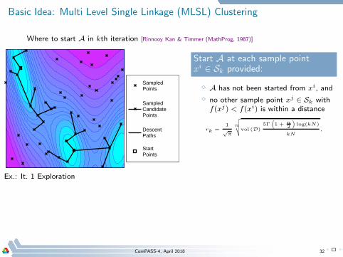
Basic Idea: Multi Level Single Linkage (MLSL) Clustering
Where to start A in kth iteration [Rinnooy Kan & Timmer (MathProg, 1987)]
Sampled Points
Sampled Candidate Points
Descent Paths
Start Points
Ex.: It. 1 Exploration
Start A at each sample pointxi ∈ Sk provided:
⋄ A has not been started from xi, and
⋄ no other sample point xj ∈ Sk withf(xj) < f(xi) is within a distance
rk =1
√π
n
√
√
√
√
vol (D)5Γ
(
1 + n2
)
log(kN)
kN,
ComPASS-4, April 2018 32

Basic Idea: Multi Level Single Linkage (MLSL) Clustering
Where to start A in kth iteration [Rinnooy Kan & Timmer (MathProg, 1987)]
Sampled Points
Sampled Candidate Points
Descent Paths
Start Points
Ex.: It. 1 Exploration
Start A at each sample pointxi ∈ Sk provided:
⋄ A has not been started from xi, and
⋄ no other sample point xj ∈ Sk withf(xj) < f(xi) is within a distance
rk =1
√π
n
√
√
√
√
vol (D)5Γ
(
1 + n2
)
log(kN)
kN,
Thm [RK-T]- With probability 1, MLSL will start finitely many local runs.
ComPASS-4, April 2018 32
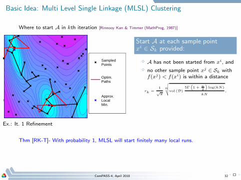
Basic Idea: Multi Level Single Linkage (MLSL) Clustering
Where to start A in kth iteration [Rinnooy Kan & Timmer (MathProg, 1987)]
Sampled Points
Optim.Paths
Approx.LocalMin.
Ex.: It. 1 Refinement
Start A at each sample pointxi ∈ Sk provided:
⋄ A has not been started from xi, and
⋄ no other sample point xj ∈ Sk withf(xj) < f(xi) is within a distance
rk =1
√π
n
√
√
√
√
vol (D)5Γ
(
1 + n2
)
log(kN)
kN,
Thm [RK-T]- With probability 1, MLSL will start finitely many local runs.
ComPASS-4, April 2018 32
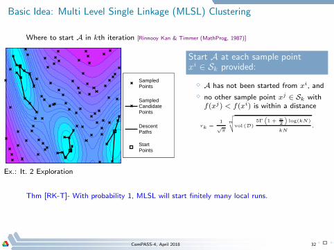
Basic Idea: Multi Level Single Linkage (MLSL) Clustering
Where to start A in kth iteration [Rinnooy Kan & Timmer (MathProg, 1987)]
Sampled Points
Sampled Candidate Points
Descent Paths
Start Points
Ex.: It. 2 Exploration
Start A at each sample pointxi ∈ Sk provided:
⋄ A has not been started from xi, and
⋄ no other sample point xj ∈ Sk withf(xj) < f(xi) is within a distance
rk =1
√π
n
√
√
√
√
vol (D)5Γ
(
1 + n2
)
log(kN)
kN,
Thm [RK-T]- With probability 1, MLSL will start finitely many local runs.
ComPASS-4, April 2018 32
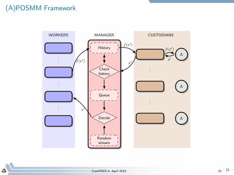
(A)POSMM Framework
History
Checkhistory
Queue
Decide
Randomstream
MANAGERWORKERS CUSTODIANS
...
...
...
...
...
A
A
A
f(x′)
x′f(x′)
x′
f(x′)
x′
ComPASS-4, April 2018 33
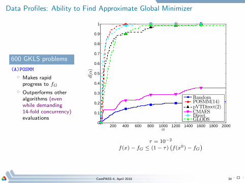
Data Profiles: Ability to Find Approximate Global Minimizer
600 GKLS problems
(A)POSMM
⋄ Makes rapidprogress to fG
⋄ Outperforms otheralgorithms (evenwhile demanding14-fold concurrency)evaluations
200 400 600 800 1000 1200 1400 1600 1800 20000
0.1
0.2
0.3
0.4
0.5
0.6
0.7
0.8
0.9
1
α
d(α)
RandomPOSMM(14)pVTDirect(2)CMAESDirectGLODS
τ = 10−2
f(x) − fG ≤ (1− τ)(
f(x0) − fG)
ComPASS-4, April 2018 34
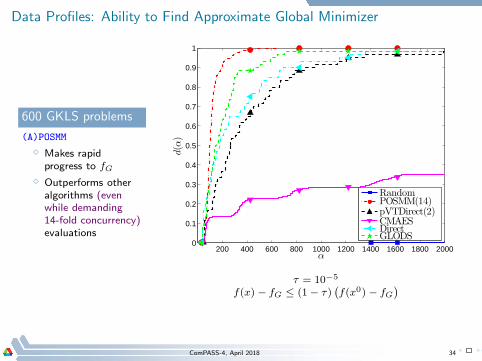
Data Profiles: Ability to Find Approximate Global Minimizer
600 GKLS problems
(A)POSMM
⋄ Makes rapidprogress to fG
⋄ Outperforms otheralgorithms (evenwhile demanding14-fold concurrency)evaluations
200 400 600 800 1000 1200 1400 1600 1800 20000
0.1
0.2
0.3
0.4
0.5
0.6
0.7
0.8
0.9
1
α
d(α)
RandomPOSMM(14)pVTDirect(2)CMAESDirectGLODS
τ = 10−5
f(x) − fG ≤ (1− τ)(
f(x0) − fG)
ComPASS-4, April 2018 34
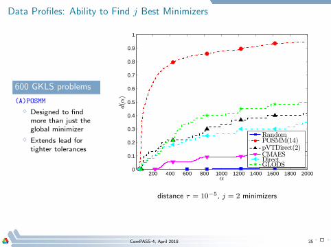
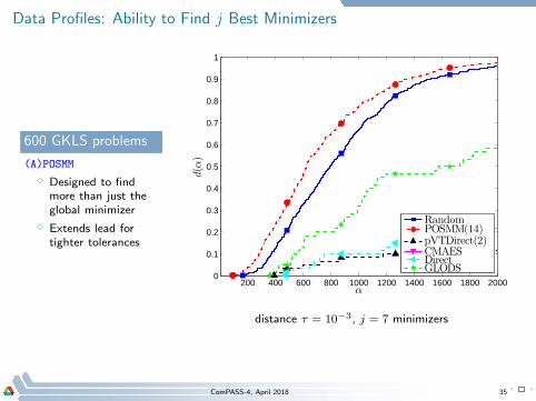
Data Profiles: Ability to Find j Best Minimizers
600 GKLS problems
(A)POSMM
⋄ Designed to findmore than just theglobal minimizer
⋄ Extends lead fortighter tolerances
200 400 600 800 1000 1200 1400 1600 1800 20000
0.1
0.2
0.3
0.4
0.5
0.6
0.7
0.8
0.9
1
α
d(α)
RandomPOSMM(14)pVTDirect(2)CMAESDirectGLODS
distance τ = 10−5, j = 2 minimizers
ComPASS-4, April 2018 35
Data Profiles: Ability to Find j Best Minimizers
600 GKLS problems
(A)POSMM
⋄ Designed to findmore than just theglobal minimizer
⋄ Extends lead fortighter tolerances
200 400 600 800 1000 1200 1400 1600 1800 20000
0.1
0.2
0.3
0.4
0.5
0.6
0.7
0.8
0.9
1
α
d(α)
RandomPOSMM(14)pVTDirect(2)CMAESDirectGLODS
distance τ = 10−3, j = 7 minimizers
ComPASS-4, April 2018 35
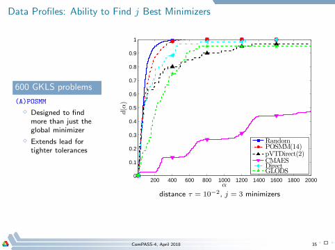
Data Profiles: Ability to Find j Best Minimizers
600 GKLS problems
(A)POSMM
⋄ Designed to findmore than just theglobal minimizer
⋄ Extends lead fortighter tolerances
200 400 600 800 1000 1200 1400 1600 1800 20000
0.1
0.2
0.3
0.4
0.5
0.6
0.7
0.8
0.9
1
α
d(α)
RandomPOSMM(14)pVTDirect(2)CMAESDirectGLODS
distance τ = 10−2, j = 3 minimizers
ComPASS-4, April 2018 35
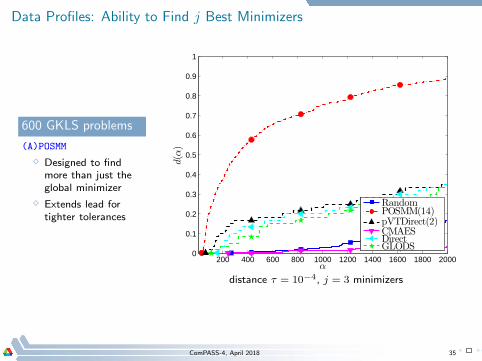
Data Profiles: Ability to Find j Best Minimizers
600 GKLS problems
(A)POSMM
⋄ Designed to findmore than just theglobal minimizer
⋄ Extends lead fortighter tolerances
200 400 600 800 1000 1200 1400 1600 1800 20000
0.1
0.2
0.3
0.4
0.5
0.6
0.7
0.8
0.9
1
α
d(α)
RandomPOSMM(14)pVTDirect(2)CMAESDirectGLODS
distance τ = 10−4, j = 3 minimizers
ComPASS-4, April 2018 35
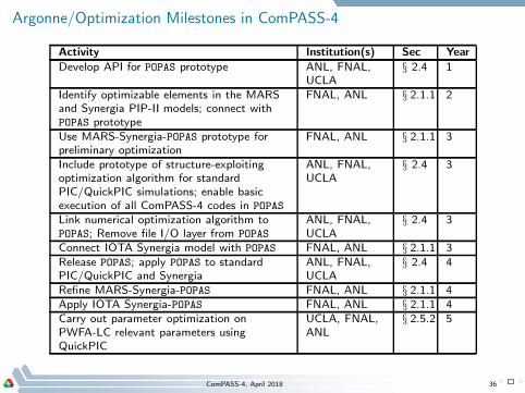
Argonne/Optimization Milestones in ComPASS-4
Activity Institution(s) Sec Year
Develop API for POPAS prototype ANL, FNAL,UCLA
§ 2.4 1
Identify optimizable elements in the MARSand Synergia PIP-II models; connect withPOPAS prototype
FNAL, ANL § 2.1.1 2
Use MARS-Synergia-POPAS prototype forpreliminary optimization
FNAL, ANL § 2.1.1 3
Include prototype of structure-exploitingoptimization algorithm for standardPIC/QuickPIC simulations; enable basicexecution of all ComPASS-4 codes in POPAS
ANL, FNAL,UCLA
§ 2.4 3
Link numerical optimization algorithm toPOPAS; Remove file I/O layer from POPAS
ANL, FNAL,UCLA
§ 2.4 3
Connect IOTA Synergia model with POPAS FNAL, ANL § 2.1.1 3Release POPAS; apply POPAS to standardPIC/QuickPIC and Synergia
ANL, FNAL,UCLA
§ 2.4 4
Refine MARS-Synergia-POPAS FNAL, ANL § 2.1.1 4Apply IOTA Synergia-POPAS FNAL, ANL § 2.1.1 4Carry out parameter optimization onPWFA-LC relevant parameters usingQuickPIC
UCLA, FNAL,ANL
§ 2.5.2 5
ComPASS-4, April 2018 36