Embed Size (px)
Citation preview
gloskip=
Optimization of a Statistical Arbitrage Strategy using theGenetic Algorithm
António Pedro de Oliveira Alcobia Vassalo Lourenço
Thesis to obtain the Master of Science Degree in
Information Systems and Computer Engineering
Supervisor(s): Prof. Rui Fuentecilla Maia Ferreira Neves
Examination Committee
Chairperson: Prof. José Luís Brinquete BorbinhaSupervisor: Prof. Rui Fuentecilla Maia Ferreira Neves
Member of the Committee: Prof. Luís Manuel Silveira Russo
September 2020

ii

Acknowledgments
I would like to thank my parents, my brothers and sister, my girlfriend, the rest of my family and friends,
and professor Rui Neves for their support during the development of this work.
iii

iv

Resumo
Esta tese explora a optimizacao de uma proposta de um sistema que gera sinais de negociacao
baseado em princıpios de arbitragem estatıstica. A optimizacao e feita usando o algoritmo genetico.
Este trabalho tambem reve a crescente literatura em arbitragem estatıstica, origem, pincıpios, evolucao
e estrategias. O sistema proposto usa dados historicos de mercado entre 2012 e 2018 para gerar back-
tests, tendo os resultados optimizados gerado um retorno anual de 12 por cento e um Sharp Ratio de
1.82.
Palavras-chave: Algoritm Genetico, Arbitragem Estatıstica, Mercados Financeiros
v

vi

Abstract
This work explores the optimization of a proposed system that generates trade signals based on statis-
tical arbitrage principles. The optimization is done using the Genetic Algorithm. This thesis also reviews
the growing literature on statistical arbitrage origin, evolution, and strategies. The system uses histor-
ical market data from 2012 to 2018 to perform the backtests, with the optimized results generating an
average return of 12 percent per anum and a Sharp Ratio of 1.82.
Keywords: Genetic Algorithm, Statistical Arbitrage, Financial Markets
vii

viii

Contents
Acknowledgments . . . . . . . . . . . . . . . . . . . . . . . . . . . . . . . . . . . . . . . . . . . iii
Resumo . . . . . . . . . . . . . . . . . . . . . . . . . . . . . . . . . . . . . . . . . . . . . . . . . v
Abstract . . . . . . . . . . . . . . . . . . . . . . . . . . . . . . . . . . . . . . . . . . . . . . . . . vii
List of Tables . . . . . . . . . . . . . . . . . . . . . . . . . . . . . . . . . . . . . . . . . . . . . . xi
List of Figures . . . . . . . . . . . . . . . . . . . . . . . . . . . . . . . . . . . . . . . . . . . . . xiii
Nomenclature . . . . . . . . . . . . . . . . . . . . . . . . . . . . . . . . . . . . . . . . . . . . . . xv
Glossary . . . . . . . . . . . . . . . . . . . . . . . . . . . . . . . . . . . . . . . . . . . . . . . . xvii
1 Introduction 1
1.1 Motivation . . . . . . . . . . . . . . . . . . . . . . . . . . . . . . . . . . . . . . . . . . . . . 2
1.2 Topic Overview . . . . . . . . . . . . . . . . . . . . . . . . . . . . . . . . . . . . . . . . . . 2
1.3 Objectives . . . . . . . . . . . . . . . . . . . . . . . . . . . . . . . . . . . . . . . . . . . . . 3
1.4 Thesis Outline . . . . . . . . . . . . . . . . . . . . . . . . . . . . . . . . . . . . . . . . . . 4
2 Background and Related Work 5
2.1 Background . . . . . . . . . . . . . . . . . . . . . . . . . . . . . . . . . . . . . . . . . . . . 6
2.1.1 Financial instruments – Stocks, Derivatives, and Futures . . . . . . . . . . . . . . . 6
2.1.2 Indexes and Futures . . . . . . . . . . . . . . . . . . . . . . . . . . . . . . . . . . . 6
2.1.3 Origin of arbitrage . . . . . . . . . . . . . . . . . . . . . . . . . . . . . . . . . . . . 6
2.2 Related Work . . . . . . . . . . . . . . . . . . . . . . . . . . . . . . . . . . . . . . . . . . . 7
2.2.1 Technical Analysis . . . . . . . . . . . . . . . . . . . . . . . . . . . . . . . . . . . . 7
2.2.2 Optimization Techniques . . . . . . . . . . . . . . . . . . . . . . . . . . . . . . . . . 9
2.2.3 Pairs Trading and Arbitrage . . . . . . . . . . . . . . . . . . . . . . . . . . . . . . . 14
3 Implementation 21
3.1 System Overview Architecture . . . . . . . . . . . . . . . . . . . . . . . . . . . . . . . . . 22
3.2 Algorithmic Trading Module . . . . . . . . . . . . . . . . . . . . . . . . . . . . . . . . . . . 23
3.2.1 Data Curation . . . . . . . . . . . . . . . . . . . . . . . . . . . . . . . . . . . . . . . 23
3.2.2 Feature Analysis . . . . . . . . . . . . . . . . . . . . . . . . . . . . . . . . . . . . . 24
3.2.3 Strategy . . . . . . . . . . . . . . . . . . . . . . . . . . . . . . . . . . . . . . . . . . 25
3.2.4 Backtest . . . . . . . . . . . . . . . . . . . . . . . . . . . . . . . . . . . . . . . . . . 27
3.3 Optimization Module . . . . . . . . . . . . . . . . . . . . . . . . . . . . . . . . . . . . . . . 27
ix
3.4 Visualization Module . . . . . . . . . . . . . . . . . . . . . . . . . . . . . . . . . . . . . . . 30
3.5 Computational optimizations . . . . . . . . . . . . . . . . . . . . . . . . . . . . . . . . . . 30
3.6 Data Used . . . . . . . . . . . . . . . . . . . . . . . . . . . . . . . . . . . . . . . . . . . . . 31
4 Studies and Validation 33
4.1 Study 1 – Calibration efficiency . . . . . . . . . . . . . . . . . . . . . . . . . . . . . . . . . 34
4.1.1 Hypothesis . . . . . . . . . . . . . . . . . . . . . . . . . . . . . . . . . . . . . . . . 34
4.1.2 Experiments . . . . . . . . . . . . . . . . . . . . . . . . . . . . . . . . . . . . . . . 34
4.1.3 Results . . . . . . . . . . . . . . . . . . . . . . . . . . . . . . . . . . . . . . . . . . 36
4.1.4 Limitations . . . . . . . . . . . . . . . . . . . . . . . . . . . . . . . . . . . . . . . . 39
4.2 Study 2 – Cointegration usage efficiency . . . . . . . . . . . . . . . . . . . . . . . . . . . . 39
4.2.1 Hypothesis . . . . . . . . . . . . . . . . . . . . . . . . . . . . . . . . . . . . . . . . 39
4.2.2 Experiments . . . . . . . . . . . . . . . . . . . . . . . . . . . . . . . . . . . . . . . 40
4.2.3 Results . . . . . . . . . . . . . . . . . . . . . . . . . . . . . . . . . . . . . . . . . . 42
4.2.4 Limitations . . . . . . . . . . . . . . . . . . . . . . . . . . . . . . . . . . . . . . . . 43
4.3 Study 3 – Strategy comparison against similar portfolios . . . . . . . . . . . . . . . . . . . 43
4.3.1 Hypothesis . . . . . . . . . . . . . . . . . . . . . . . . . . . . . . . . . . . . . . . . 43
4.3.2 Experiments . . . . . . . . . . . . . . . . . . . . . . . . . . . . . . . . . . . . . . . 44
4.3.3 Results . . . . . . . . . . . . . . . . . . . . . . . . . . . . . . . . . . . . . . . . . . 44
4.3.4 Limitations . . . . . . . . . . . . . . . . . . . . . . . . . . . . . . . . . . . . . . . . 46
5 Conclusions 47
5.1 Achievements . . . . . . . . . . . . . . . . . . . . . . . . . . . . . . . . . . . . . . . . . . . 48
5.2 Future Work . . . . . . . . . . . . . . . . . . . . . . . . . . . . . . . . . . . . . . . . . . . . 48
Bibliography 49
x

List of Tables
2.1 Comparison of strategies statistics between different authors . . . . . . . . . . . . . . . . 19
3.1 Extract of one of the CSV with historical market data . . . . . . . . . . . . . . . . . . . . . 31
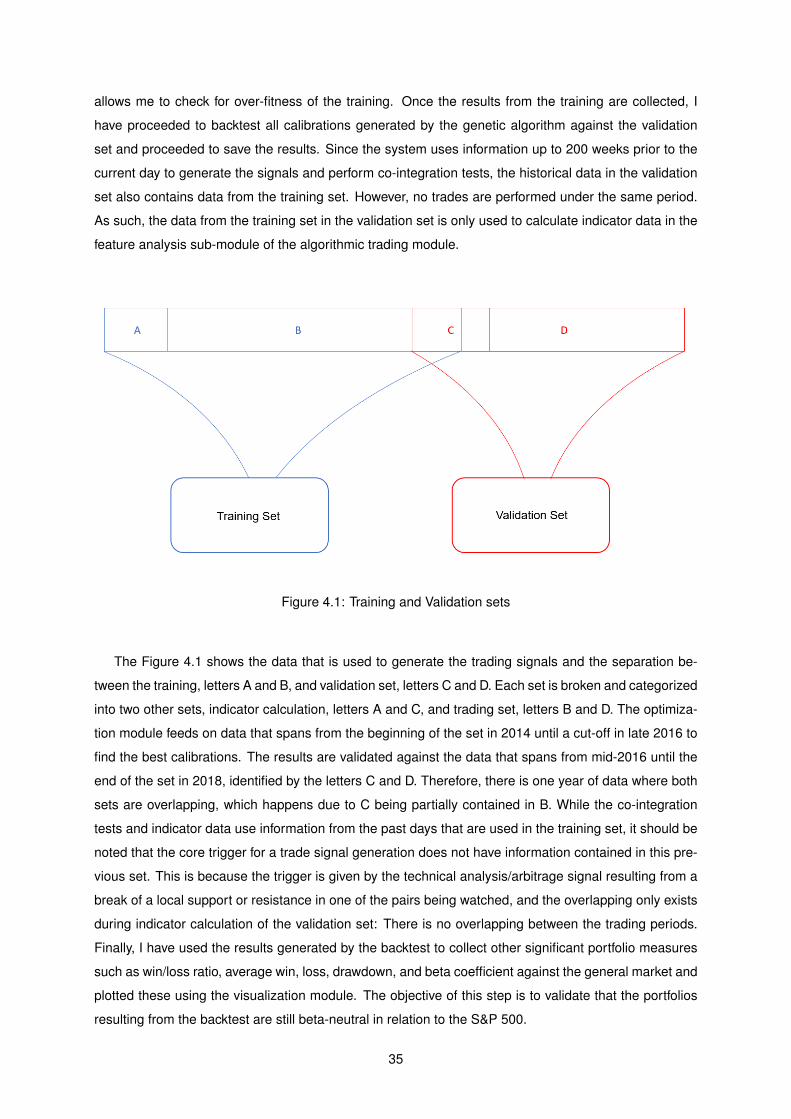
4.1 Random calibrations portfolio statistics . . . . . . . . . . . . . . . . . . . . . . . . . . . . . 36
4.2 Best calibrations found . . . . . . . . . . . . . . . . . . . . . . . . . . . . . . . . . . . . . . 37
4.3 Proposed system statistics VS S&P 500 . . . . . . . . . . . . . . . . . . . . . . . . . . . . 44
4.4 Ranking of strategies statistics between different authors and proposed solution . . . . . 45
xi

xii

List of Figures
2.1 Example of a Support . . . . . . . . . . . . . . . . . . . . . . . . . . . . . . . . . . . . . . 8
2.2 Examples of three moving averages . . . . . . . . . . . . . . . . . . . . . . . . . . . . . . 8
2.3 Example of Bollinger Bands . . . . . . . . . . . . . . . . . . . . . . . . . . . . . . . . . . . 9
2.4 Example of a Neural Network . . . . . . . . . . . . . . . . . . . . . . . . . . . . . . . . . . 10
2.5 Example of the inner structure of a node . . . . . . . . . . . . . . . . . . . . . . . . . . . . 10
2.6 An example of an Elman Network . . . . . . . . . . . . . . . . . . . . . . . . . . . . . . . . 11
2.7 Example of Crossover and Mutation operations . . . . . . . . . . . . . . . . . . . . . . . . 13
2.8 Example of pairs moving together . . . . . . . . . . . . . . . . . . . . . . . . . . . . . . . 16
2.9 Arbitrage Strategies Classification . . . . . . . . . . . . . . . . . . . . . . . . . . . . . . . 18
3.1 Proposed System Architecture Overview . . . . . . . . . . . . . . . . . . . . . . . . . . . . 22
3.2 Example of Resampling and tradable intervals matching in the Data Curation sub-module 24
3.3 Example of three signals given by the high-lows strategy . . . . . . . . . . . . . . . . . . . 25
3.4 Calculated index and it’s moving averages . . . . . . . . . . . . . . . . . . . . . . . . . . . 26
3.5 Highlight of trades in the purposed system . . . . . . . . . . . . . . . . . . . . . . . . . . . 26
3.6 Optimization module Overview . . . . . . . . . . . . . . . . . . . . . . . . . . . . . . . . . 28
3.7 Extract of code with the calibration function . . . . . . . . . . . . . . . . . . . . . . . . . . 29
3.8 Labeling of the encoded genes . . . . . . . . . . . . . . . . . . . . . . . . . . . . . . . . . 29
4.1 Training and Validation sets . . . . . . . . . . . . . . . . . . . . . . . . . . . . . . . . . . . 35
4.2 Optimization Results in Training VS Validation sets . . . . . . . . . . . . . . . . . . . . . . 37
4.3 Optimized Portfolio Weekly Returns VS S&P 500 Weekly Returns . . . . . . . . . . . . . 38
4.4 Average performance by cointegration cut-off . . . . . . . . . . . . . . . . . . . . . . . . . 40
4.5 Portfolios P&L evolution by cointegration cut-off . . . . . . . . . . . . . . . . . . . . . . . . 41
4.6 Generated index evolution by cointegration cut-off . . . . . . . . . . . . . . . . . . . . . . 42
xiii

xiv

Nomenclature
Greek symbols
α Linear independent vectors.
β Coefficient between pairs of stocks.
ε Stochastic process error.
Σ Sum.
xv

xvi
Glossary
ADF Augmented Dickey-Fuller test - The test can be used to test for a unit root in a univariate process
in the presence of serial correlation.. 30
APT Arbitrage Price Theory - A pricing model that predicts a return using the relationship between an
expected return and macroeconomic factors. 1
BB Short for Bollinger Bands. 9
EMH Efficient Market Hypothesis - An investment theory that states that share prices reflect all available
information. 1
EOD End of Day - Closure of the stock market. 16
Legs Leg - A trade might be composed by individual bets, each called a leg.. 2
Long Long Position - A speculative bet aiming to profit at the rise of stock prices. 2
MAs Short for Moving Averages. 7
RWH Random Walk Hypothesis - An investment theory that states that share prices evolve following a
random walk. 1
Short Short Position - A speculative bet aiming to profit at the downfall of stock prices. 2
Tick Tick - Small variation possible in the price of an instrument. 17
xvii

xviii

Chapter 1
Introduction
The stock market plays an important role in the economy of a country. Not only it does increase the
transparency of corporations raising trust among investors, but it also provides an important role by
allowing companies to re-finance and increasing the liquidity and efficiency of that countries market. By
tracking the value of public companies, the stock market has also become an important indicator of a
country’s economy. Due to the strong correlation between a country’s stock market and it’s economy
and the potential financial opportunities it generates, predicting the price movements has become one
of the main focuses on the interest in this area. Due to the nature of the markets, these are highly noisy
systems under the influence of various forces, either economic, political, or natural disasters. This makes
predicting price movements extremely hard. Various techniques were developed to tackle this task, and
they can be divided into two main groups: Technical analysis, which studies past price movements and
volume to try to predict the future, and fundamental analysis, which focus on how external factors, such
as politics or economics, might impact the market prices. Opposing these techniques, theories such
as Efficient Market Hypothesis (EMH), which believes prices reflect all the information in the market,
have a better acceptance among scholars. Based on this theory, others such as the Random Walk
Hypothesis (RWH), which states that prices evolve according to a random walk, have been developed.
Other theories, such as the Arbitrage Pricing Theory (APT) in which this work is based on, believe
that markets can be forecast to some degree, opposing the EMH and RWH theories mentioned above,
have later on emerged and been also acceptable by scholars. With the advent of computer trading and
the evolution of quantitative strategies, there has been a big attraction from the Artificial Intelligence
community to explore possible applications in this area.
1

1.1 Motivation
Investors with large pools of capital face difficult challenges in deployment and allocating capital across
investments with uncorrelated risk since most products and investments available have some level of
correlation to the economy and global indexes returns. As history often repeats itself and stock mar-
ket crashes happen, investors have been developing an interest in strategies in which returns are not
correlated with the general market direction. These are called market-neutral or beta-neutral strategies.
Based on this principle, one type of strategies that have gain significant popularity is the pairs trading,
or statistical arbitrage. Pairs trading focuses on the principle of using a collection of stocks to create
various Legs of a single trade. Some of these legs are Long while others are Short, working as an
hedge. The pair’s selection is based on statistical tests such as co-integration to check for the existence
of share hidden variables between the pairs. It is of interest to explore how we can apply machine learn-
ing optimization techniques, such as the genetic algorithm, to optimize and create new trading strategies
based on these market-neutral principles.
1.2 Topic Overview
This work begins by reviewing the literature on statistical arbitrage systems and how these have evolved
over time. The systems are explored and categorized based on the techniques used. The techniques
used in these systems are then explored, with a focus on arbitrage theory and artificial intelligence. In
this work, I also have architecture and developed a system that is capable of taking market data and gen-
erate trading signals based on a series of parameters provided. The system works by combining infor-
mative signals from a simple statistical arbitrage strategy based on technical analysis and co-integration
testing to generate a tradable signal. The backtest consists of applying a simple trend-following strategy
to this tradable signal and saving the results. Since there are millions of possible different combinations
to configure the system, I use an artificial intelligence technique, the genetic algorithm, to find an opti-
mal calibration. This process involves performing several backtests with different possible calibrations
in separate training and validation sets with the sharp ratio as the ranking function. The training set is
used to determine the best individuals, while the validation set is used to validate the results and control
for over fitness. Three experiments are conducted using this system to validate the hypothesis that we
can use artificial intelligence techniques to improve simple statistical arbitrage trading strategies: The
resulting calibration of the genetic algorithm is compared with random calibrations. The co-integration
used for filtering purposes is tested using different cut-offs. The performance of the strategy is compared
against other statistical arbitrage and artificial intelligence-based trading strategies.
2
1.3 Objectives
The goal of this work is to explore the usage of artificial intelligence, market analysis, and arbitrage
price theory. It is expected to produce an application capable of generating investment signals in the
stock market, producing a portfolio with beta-neutral returns. This application requires a series of inputs
used in the calculation of indicators and cut-off rates for statistical tests. The objective is, using the
Genetic Algorithm, to find appropriate calibrations for this application, which result in an optimization of
the generated portfolios returns when adjusted for risk-metrics such as portfolio deviation, drawdown,
and beta-neutrality.
As such, the objectives of this thesis are:
• Explore beta-neutral trading strategies with a focus on pairs-trading.
• Explore the usage of technical analysis for the generation of trading signals.
• Explore how machine learning is being used to improve and deploy beta-neutral trading strategies.
• Parse and pair stock information of US companies to be used in pairs-trading.
• Create a system capable of generating investment decisions in the form of explicit trading signals.
• Calibrate the system using the genetic algorithm.
• Study the resulting performance against the S&P 500 and similar systems.
• Explore computer optimization techniques in order to be able to process vast amounts of data
generated by the combination of stock pairs.
This thesis presents the following contributions:
• Develop a beta-neutral system based on technical analysis and pairs trading that takes in a series
of inputs and is capable of generating profitable trading signals;
• Assemble a Genetic Algorithm that backtests possible sets of inputs for the system and generates
suggested configurations.
• Explore how sensible are the portfolio returns against changes in the co-integration tests that hold
fundamental premises of the strategy.
3

1.4 Thesis Outline
This work is divided into the following five main chapters:
• Chapter 1 – Introduction – Here, an overview of this work is given along with its motivation, goals,
and contributions.
• Chapter 2 – Background – A literature review is done in this chapter where the evolution of beta-
neutral strategies and the artificial intelligence techniques used in them are explored. Technical
analysis concepts are also introduced and explained.
• Chapter 3 – Architecture and System – Begins with a brief overview of the system that was devel-
oped, followed by an in-depth dive into each component of the system.
• Chapter 4 – Experiments and Validation – Three studies made possible using the system described
in Chapter 3 are presented and validated.
• Chapter 5 – Conclusion – In this chapter, the conclusions about the work developed and the
strategy performance are drawn. Future work propositions are presented.
4

Chapter 2
Background and Related Work
In this chapter, we present an overview of the various concepts required for the understanding of the
developed work. In the Background section, I start by reviewing the most basic components that con-
stitute the capital markets, followed by how they work and interact with each other, in this section I also
explore the concept and origin of arbitrage strategies. This is followed by a review in the Related Work,
beginning with technical analysis where the concepts of resistances and supports are introduced along
with the concepts of moving averages. Next, I review machine learning techniques and concepts that
are used on later chapters of this work, with a focus on the genetic algorithm, and in other cases that
are used in the different machine learning approaches that are explored. Finally, I explore each one
of the strategies and provide a taxonomy classification based on the principles each on having at heart
(co-integration, distance, machine learning, time-series analysis). I have also summarized the strategies
based on their returns.
5
2.1 Background
In this section I explore the base concepts and components that make up the stock market and I give an
introduction and a brief review on arbitrage and its origin.
2.1.1 Financial instruments – Stocks, Derivatives, and Futures
Accordingly to the International Accounting Standards, a financial instrument is described as ”any con-
tract that gives rise to a financial asset of one entity and a financial liability or equity instrument of
another entity” 1. Some of these financial instruments are traded publicly. In the context of this thesis,
the most important instruments to be understood are both stocks and futures. A stock represents a
portion of ownership over a corporation. In order to understand the future contracts, we need to under-
stand derivatives first. According to the US Department of Treasury, a derivative is ”a financial contract
whose value is derived from the performance of some underlying market factors, such as interest rates,
currency exchange rates, and commodity, credit, or equity prices.” 2. A future, a type of derivative, is an
agreement to trade an underlying asset on some future date, at a price that is locked in today. Future
contracts are traded anonymously on an exchange at a publicly observed market price and are generally
very liquid. [1]
2.1.2 Indexes and Futures
Charles H. Dow, in 1884, had an idea on how to communicate the overall health and performance of
the stock market: He made a weighted average of securities prices based on their market capitalization.
Since he was focusing on the transportation industry, he only picked stocks operating in that area. It was
called the Railroad Average, now known as the Dow Jones Transportation Average (DJTA). Over the
years, by using Charles Dow’s technique, other indexes start appearing. Some of them try to describe a
certain sector (such as the DJTA) or financial instrument type, while others describe the general econ-
omy (such as the Dow Jones Industrial Average - DJIA). Based on Dow’s work, futures with indexes as
underlying assets appeared and are among the most traded financial instruments in the world. Although
the traditional definition of an index persists, it is not because of its inherent superiority or economy of
implementation, but because its past success has led to inertia in considering other alternatives [2]. As
an example, some authors [5] have proposed updated variations of the DJIA that are better at tracking
the principles of Dow Theory in today’s market.
2.1.3 Origin of arbitrage
Arbitrage is, in theory, a risk-less trading strategy consisting of the buying and selling of equivalent goods
in different markets in order to take advantage of a price difference. Any situation where it is possible
to make a profit without taking any risk or making an investment is called an arbitrage opportunity.
1https://www.iasplus.com/en/standards/ias/ias32 - 27th April 20192https://www.occ.treas.gov/topics/capital-markets/financial-markets/derivatives/index-derivatives.html - 27th April 2019
6
[3] In ancient times, markets were much less efficient, which resulted in a vast number of arbitrage
opportunities. The first evidence comes from the mercantile trade in the Middle East, where the difficulty
in moving goods and the lack of information on routes created these opportunities. In more modern
times, before electronic trading was invented, discrepancies in prices for the same financial instrument
between, for example, the London Stock Exchange and the New York Stock Exchange were frequent
and created frequent arbitrage opportunities that were quickly exploited using the telegraph. This trade
was referred to as shunting [4]. Nowadays, with electronic trading, the markets are much more liquid and
efficient as the most basic arbitrage opportunities are explored in a matter of milliseconds with orders
between exchanges traveling at the speed of light. Arbitrage is a practice of historical importance since
it contributed to the development of society by increasing liquidity where it is most in need contributing
to a more efficient market and to the development of important principles such as the Law of One Price3.
2.2 Related Work
2.2.1 Technical Analysis
Technical analysis aims at forecasting the direction of prices through the study of past market data [5].
Technical analysts try to detect patterns in prices, volume, and indicators and use them to create an
overview of the market and generate their trade ideas. Technical analysts believe that the patterns
observed in the price and volume of the instruments are the result of the behavior and, thus, the psy-
chology of the other traders in the market. The efficiency of technical analysis just by itself as a source
of investment decisions is highly disputable.
Resistances and Supports
Technical analysts believe that, due to human nature, certain prices might generate a net increase in
buying or selling. Some examples of these prices are round numbers or local and global maximum and
minimum values of prices in the past. As such, changes in the direction of the price naturally create
these points of interest that should be taken into consideration as they are regarded as potential points
for a reversion of a trend. Suppose the price of a stock is falling and fails to go lower than a certain price,
then that price has become a support. Resistances are the opposite of supports [6]. They are created
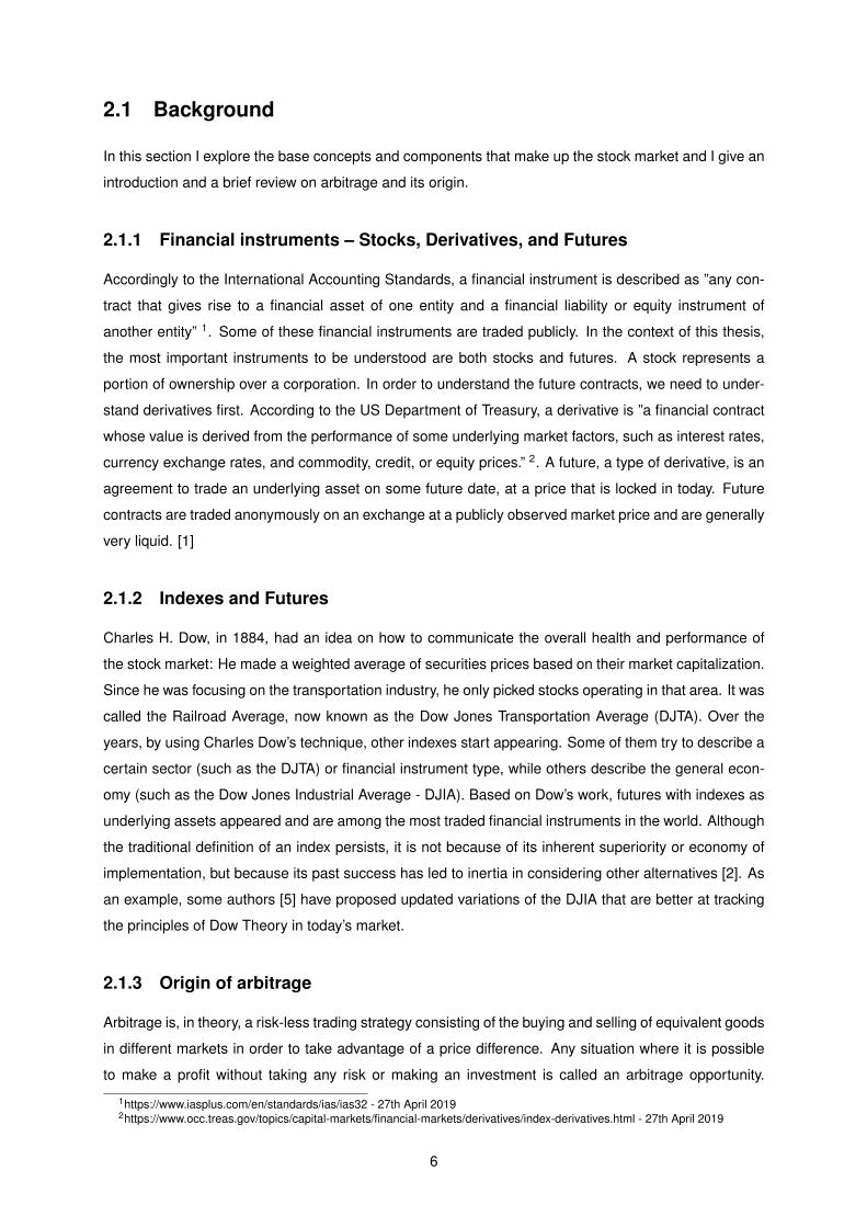
when prices fail to go higher than a certain level. An example can be see in Figure 2.1, where the price
finds a support whenever approaching parity.
Moving Averages
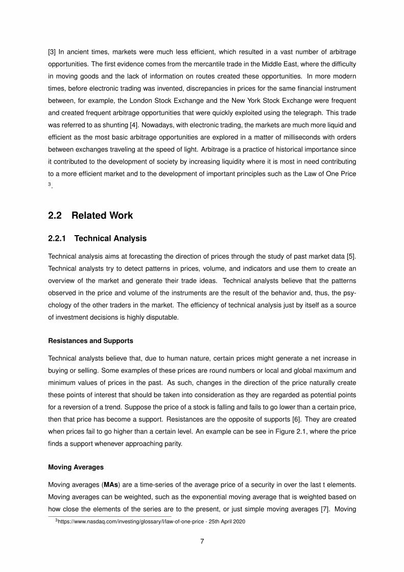
Moving averages (MAs) are a time-series of the average price of a security in over the last t elements.
Moving averages can be weighted, such as the exponential moving average that is weighted based on
how close the elements of the series are to the present, or just simple moving averages [7]. Moving3https://www.nasdaq.com/investing/glossary/l/law-of-one-price - 25th April 2020
7
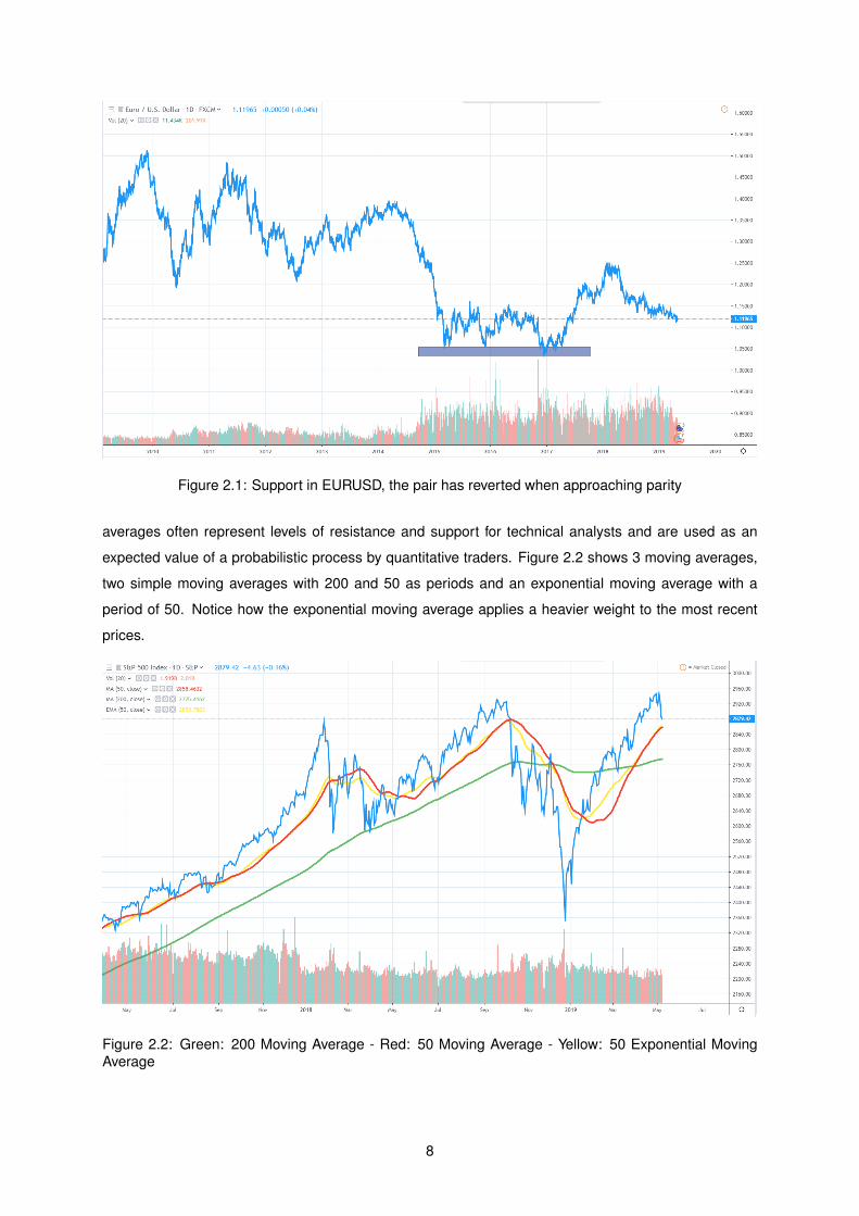
Figure 2.1: Support in EURUSD, the pair has reverted when approaching parity
averages often represent levels of resistance and support for technical analysts and are used as an
expected value of a probabilistic process by quantitative traders. Figure 2.2 shows 3 moving averages,
two simple moving averages with 200 and 50 as periods and an exponential moving average with a
period of 50. Notice how the exponential moving average applies a heavier weight to the most recent
prices.
Figure 2.2: Green: 200 Moving Average - Red: 50 Moving Average - Yellow: 50 Exponential MovingAverage
8
Other indicators
Other important indicators to be considered in this thesis are the Bollinger Bands (BB). This indicator
takes two inputs: a period for an average and a value for the standard divisions to be drawn. The
indicator calculates and provides the defined standard deviation of the average price over the period
of time defined in the first input, the price rarely surpasses the second standard deviation as shown in
Figure 2.3.
Figure 2.3: Bollinger Bands 2nd standard deviation on a 20-day MA
2.2.2 Optimization Techniques
In this section I review the literature on machine learning and techniques and algorithms that will be
used, in the context of this work, for the optimization of the statistical arbitrage strategy along with the
techniques that are used in the strategies that will be reviewed on the machine learning approaches
towards statistical arbitrage. I review the concepts of artificial neural networks, genetic algorithms and
Elman networks.
Artificial Neural Networks
As described in Haykin’s book [8], an artificial neural network (ANN) is a computing system inspired by
the biological neural networks and astrocytes that constitute animal brains. A neural network constitutes
a framework in which different machine learning algorithms can be used to process complex inputs. An
artificial neural network constitutes in a collection of nodes, also called artificial neurons, connected to
each other, forming the biological equivalent of synapses. For each node and each connection, a real
number is assigned, also called the weight. These nodes are organized into three different types of
9

layers: input, hidden, and output layers. The input layer is the one that receives our data inputs, while
the output layer is the one that returns the resulting transformations of the input data after passing on
the entire network. The hidden layer is any layer that is not an input or output layer, as shown on Figure
2.6.
Figure 2.4: An example of a neural net with an input layer with three nodes (x1, x2, x3), a hidden layerwith three nodes (z1, z2, z3), and an output layer with two nodes (o1, o2)
In Figure 2.5, we see the structure of a neuron. Each one of the arrows has a weight associated with
it that is used to multiply the incoming data to the next piece of the structure. When training a network,
we are attempting to find the best weight for each input that is able to solve our problem. Artificial neural
Figure 2.5: The inner structure of a node. F represents the activation function, which is applied to thesum of inputs)
networks function by passing a weighted sum of inputs based on each node and connection weight. F
is the activation function that will determine if this neuron is activated or not an with what value. They
are able to learn since the weights change based on how further from the solution the artificial neural
network output is. As such, it is necessary to define a loss function to calculate the distance to the
solution and then use an algorithm to adjust the weights of the network.
10
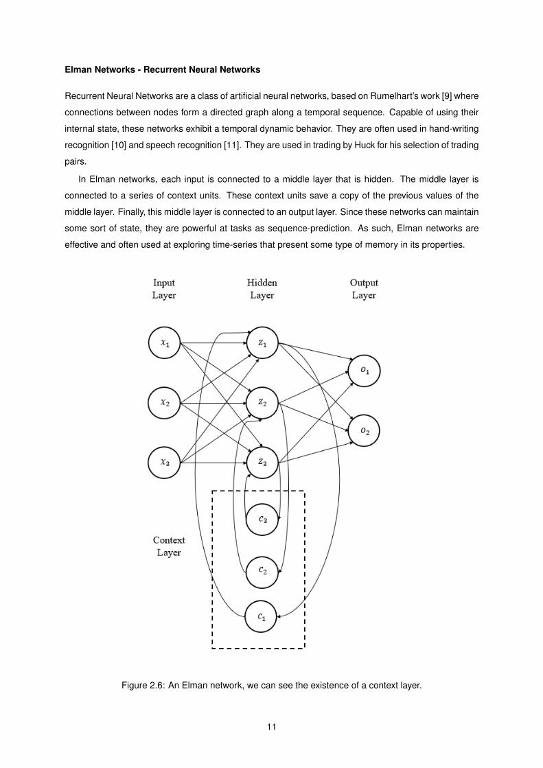
Elman Networks - Recurrent Neural Networks
Recurrent Neural Networks are a class of artificial neural networks, based on Rumelhart’s work [9] where
connections between nodes form a directed graph along a temporal sequence. Capable of using their
internal state, these networks exhibit a temporal dynamic behavior. They are often used in hand-writing
recognition [10] and speech recognition [11]. They are used in trading by Huck for his selection of trading
pairs.
In Elman networks, each input is connected to a middle layer that is hidden. The middle layer is
connected to a series of context units. These context units save a copy of the previous values of the
middle layer. Finally, this middle layer is connected to an output layer. Since these networks can maintain
some sort of state, they are powerful at tasks as sequence-prediction. As such, Elman networks are
effective and often used at exploring time-series that present some type of memory in its properties.
Figure 2.6: An Elman network, we can see the existence of a context layer.
11
Genetic Algorithms
Some authors have suggested using evolutionary algorithms [12], such as the genetic algorithm, in the
optimization of trading strategies [13] [14] [15]. which are inspired by the way natural selection and DNA
work. The principle of these algorithms is that the strongest, or in this case, best performing, individuals
survive and seed the next generation. As such, each consecutive generation is closer to full-filling the
necessary requirements and thus becoming a solution. There are two main factors for the success in
these types of algorithms: creating the right variation for the offspring and making selections towards
our solution.
Accordingly to these principles [16], each individual (chromosome) is a collection of variables (genes),
each group of individuals is called a population. The goal is to find the best collection of variables that
solve our problem. As such, it is first necessary to encode the variables that we want to optimize into
genes. In the next step, a random population is generated based on the available genes. To find the
solution, I apply a simple principle based on natural selection until the new population performance is
considered satisfactory for the problem, by following three steps iteratively:
Evaluating the best individuals - The process begins by decoding each individual’s genes into the
corresponding collection of variables. We use these variables to attempt to solve the problem at hand
and measure its performance using what is called an evaluation function. After each chromosome is
tested for its ability to solve the problem, they are ranked. Using this system, it becomes possible to
identify the best individuals in each generation.
Generate a new population - Using the best individuals from our current population, we want to
generate a new population. We want to introduce variations in the variables with the objective that each
posterior population is overall better at solving our problem. There are two ways in nature that variations
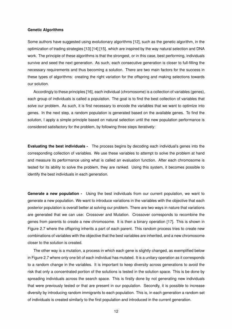
are generated that we can use: Crossover and Mutation. Crossover corresponds to recombine the
genes from parents to create a new chromosome. It is then a binary operation [17]. This is shown in
Figure 2.7 where the offspring inherits a part of each parent. This random process tries to create new
combinations of variables with the objective that the best variables are inherited, and a new chromosome
closer to the solution is created.
The other way is a mutation, a process in which each gene is slightly changed, as exemplified below
in Figure 2.7 where only one bit of each individual has mutated. It is a unitary operation as it corresponds
to a random change in the variables. It is important to keep diversity across generations to avoid the
risk that only a concentrated portion of the solutions is tested in the solution space. This is be done by
spreading individuals across the search space. This is firstly done by not generating new individuals
that were previously tested or that are present in our population. Secondly, it is possible to increase
diversity by introducing random immigrants to each population. This is, in each generation a random set
of individuals is created similarly to the first population and introduced in the current generation.
12
Figure 2.7: Crossover and mutation example over one byte
Population replacement - The process begins by decoding each individual’s genes into the corre-
sponding collection of variables. We use these variables to attempt to solve the problem at hand and
measure its performance using what is called an evaluation function. After each chromosome is tested
for its ability to solve the problem they are ranked. Using this system, it becomes possible to identify the
best individuals in each generation.
The newly generated population is then used to substitute individuals from the previous population.
Not all individuals need to be substituted. There are different techniques that can be used to perform
these selections, being the most common:
Generational selection: No individuals from previous generations are kept. The new generation
is the new population generated at each iteration.
Steady-state selection: In this selection, all individuals that were generated, the offspring, and the
individuals that were used to generate the offspring, the parents, are selected for the new generation.
The individuals that were not used are discarded.
Elitist selection: Only the best individuals from each generation are used in combination with the
newly generated ones. The best individuals are the ones that scored the highest rank in the evaluation
step. This selection has the advantage of making sure that the best individuals are not lost between
generations.
Tournament selection: The individuals are randomly split into subgroups. The Tournament selec-
tion is applied to each subgroup, and only the fittest survive [18].
Fitness proportional selection: Each individual inside each population can be ranked on how
they fit relatively to its population. For example, we could pick only individuals who are one standard
deviation above from the mean. We can apply different ranking functions, calling this a ranking selection.
13
2.2.3 Pairs Trading and Arbitrage
In this section, the concept of arbitrage is studied along with its origins and evolution. Different types
of arbitrage approaches are then analyzed and categorized in accordance with the current literature.
Finally, different strategies using the different approaches are put into comparison. We follow Krauss
[10] taxonomy of arbitrage strategies and compile other different arbitrage strategies that seem relevant
for my purposed solution.
Arbitrage strategies - Distance approach
The distance approach sets a set of pre-determined rules based on the distance between financial in-
struments to generate its trades. According to the creator of the strategy [19], certain stocks might share
a weakly dependence over a certain time period, based on Bossaerts work [20], that finds evidence of
price co-integration for US stocks. This interpretation implies that certain stocks move together not be-
cause of coincidence but because they are a product of individual integration (in the time series sense),
and some linear combination of them have a lower order integration. We can also have an intuitive
approach on this matter: On a fundamental level, stocks in the US share identical underlying variables
or share a determined sector, so it is expected that some level of correlation exists. This interpretation
implies that certain assets are weakly redundant, and when there is a deviation of their price from the
linear combination of prices in other assets, it is expected to be temporary and reverting. Based on this
assumption, an observation period begins for one year, where the cumulative returns of each stock are
tracked. These returns take into account factors such as dividends and dividend re-investments. The
top 20 pairs of pairs that minimize the sum of squared deviations between the two normalized price
series are put on a trading watch list for six months. These values were chosen arbitrarily. Whenever a
difference of two-standard deviation spread was observed, the pair was traded, one long and the other
short, until prices converged. This strategy has demonstrated a return of 11% year over year during a
40-year period, with very little correlation between its results and the overall market. Due to Gatev et al.
interpretation of the pair’s price time series as co-integrated in the sense of Bossaerts, there is some
criticism on this strategy forming period. Since no actual co-integration test is made and too often high
correlation is not related to a co-integration relationship, Do and Faff [21] confirmed that in 32% of the
time, the distance pairs did not converge. They also showed that co-integration more frequently exhibits
mean-reverting behavior compared to distance pairs and purposed, and by refining the selection criteria,
it is possible to generate similar results with less volatility. Some of the refinements consisted of creating
portfolios based on industries and favoring pairs with a high number of zero-crossings in the formation
period. Although this approach strategy has little relevance for the creation of our purposed solution, it
set an important step in statistical arbitrage trading.
14
Arbitrage strategies - Cointegration approach
Vidyamurthy in his book [22] provides us a theoretical framework for co-integration based pairs trading,
his work is one of the most cited in the area. The author suggests a selection of financial instruments
based on fundamental and statistical analysis followed by a tradeability assessment based on Engle-
Granger [21] co-integration test. Their trade signals are generated with non-parametric methods.
Other authors have studied and compared the usage of other co-integration tests. They have shown
that it is possible to achieve similar and even better results depending on a case-to-case basis.
I briefly explain Engler-Granger co-integration test and how Boassaerts applied it to stocks since it is
the most used in the approaches I reference:
According with this method, if two time-series are non-stationary and integrated of order 1, then a
linear combination of them must be stationary:
yt − βxt = ut (2.1)
In this case,
ut (2.2)
is a stationary time-series. Bossaerts [23] applies this principle to stocks, he supposes that prices
obey a statistical model of the form:
pit =∑
βitplt + εit, k < n (2.3)
Where
εit (2.4)
denotes a weakly dependent error
pit (2.5)
is weakly dependent after differentiating once. Under these assumptions and according with Engle
and Granger [21] and Bossaerts [23], the price vectors
pt (2.6)
is co-integrated of order 1 with co-integrating rank r=n-k, thus, there exists r linearly independent
vectors
{αq}q=1..r (2.7)
such that
15
zq = αq‘pt (2.8)
are weakly dependent.
For a list of potential co-integration tests I refer to Krauss [24], where we see different authors try to
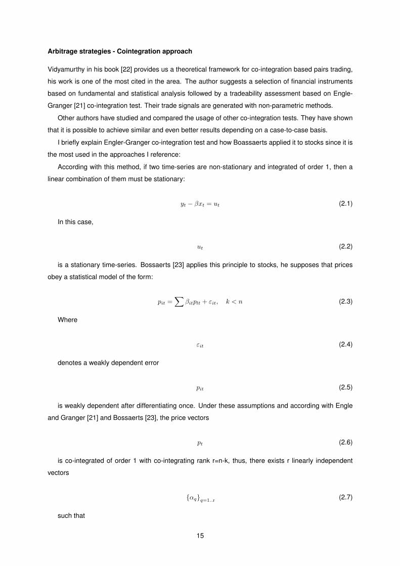
apply co-integration strategies in US markets. Huck and Afawubo [25] confirmed that the co-integration
approach significantly outperforms the distance approach for the index S&P 500.
Figure 2.8: S&P 500 (in blue) VS Dow Jones (in orange) Cumulative Returns, we can see how thesetwo indexes move together.
Arbitrage strategies - Time-Series approach
Elliott et al. [26] introduced state-space models and appropriate estimation algorithms to parametrically
deal with mean-reverting spreads. He describes the spread as a mean-reverting Gaussian Markov chain
observed in Gaussian noise. He has shown that according to his model, it is possible to describe the
state model as an Ornstein-Uhlenbeck process. Although Elliott’s work gives us a framework to work
with, it lacks practical implementation. Avellaneda and Lee [27] successfully apply a variant of this
approach to mean-reverting portfolios developed using principal component analysis (PCA) to extract
the most important factors from the market data. This application clearly indicates that dynamic trading
rules based on time-series analysis can improve trading returns. Another important mention is that in
this work, Avellaneda presented results that suggested that ”volume information is valuable in the mean-
reversion context, even at the EOD timescale”. PCA is an algorithm often used in Machine Learning for
feature reduction.
16
Arbitrage strategies - Machine Learning approach
The most relevant works in this area in our context are from Huck [28], Takeuchi and Lee [29], and
finally, Dixon [30]. Instead of using quadratic distance or co-integration tests mentioned above, Huck
in 2009[19], uses Elman networks (Recurrent Neural Networks) to generate potential trading pairs. He
then uses the Electre III algorithm to generate a decision matrix taking long and short positions based
on the stock’s ranking position.
Takeuchi and Lee [29] have shown that it is possible to use deep learning for momentum trading
strategies with the use of an autoencoder and feedforward neural networks (FFNN). Their approach is
similar to the one used by Hinton and Salakhutdinov [31] for hand-written digits classification.
Trading momentum can be applied to more than just single stocks. It is possible to trade the mo-
mentum of our own generated signals, which can be, for example, the spread between securities in our
arbitrage trading model. As such, it might be useful for the identification of a reversion to the mean.
Using a similar algorithm, Dixon [30] managed to demonstrate a 73% accuracy on the direction
prevision of an instrument. This author, however, was focusing on a much smaller timescale: 5-minute
Ticks instead of the daily and monthly inputs for Takeuchi and Lee. He also was aggregating the data
across multiple instruments and signals instead of individual instruments, which required a much more
efficient implementation by using state-of-the-art parallel computing.
While a processor-specific optimization is beyond this work scope, it is important to keep in mind of
this constraint when working with very short time frames. As such, we won’t explore arbitrage opportu-
nities in a time scale lower than one minute.
17
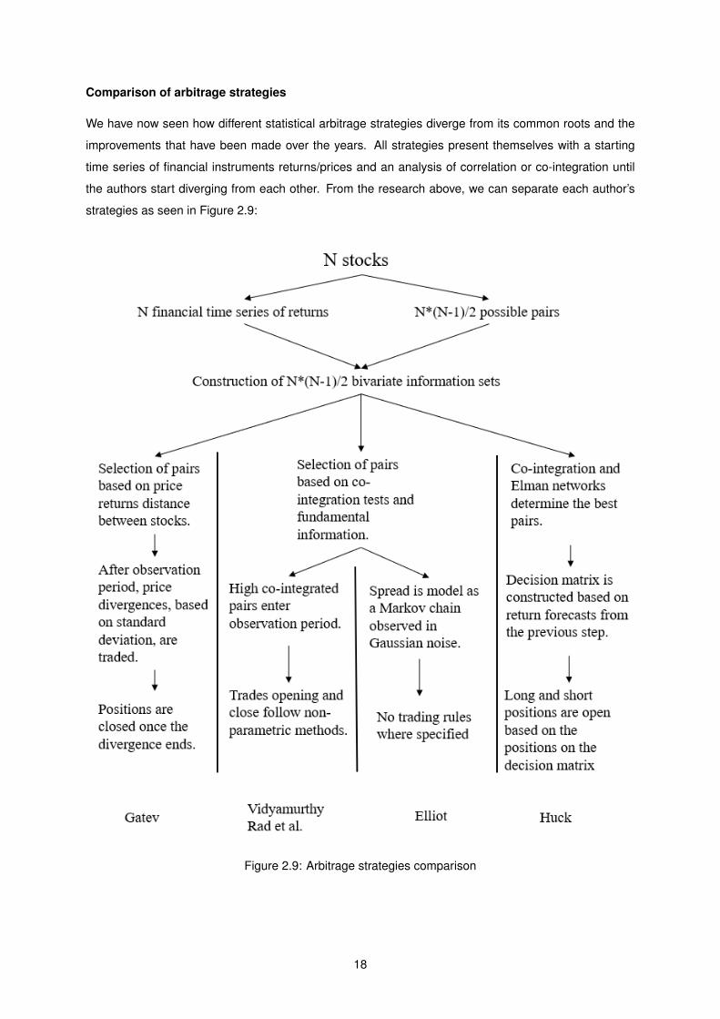
Comparison of arbitrage strategies
We have now seen how different statistical arbitrage strategies diverge from its common roots and the
improvements that have been made over the years. All strategies present themselves with a starting
time series of financial instruments returns/prices and an analysis of correlation or co-integration until
the authors start diverging from each other. From the research above, we can separate each author’s
strategies as seen in Figure 2.9:
Figure 2.9: Arbitrage strategies comparison
18
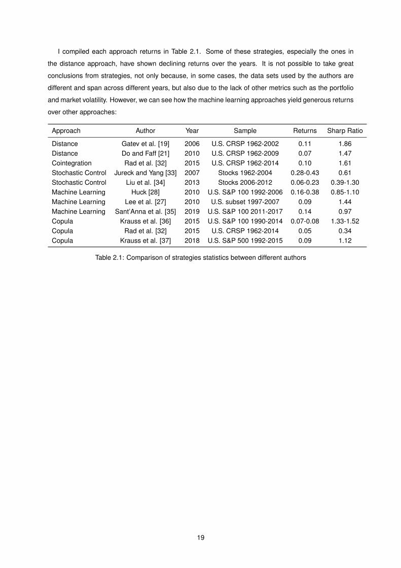
I compiled each approach returns in Table 2.1. Some of these strategies, especially the ones in
the distance approach, have shown declining returns over the years. It is not possible to take great
conclusions from strategies, not only because, in some cases, the data sets used by the authors are
different and span across different years, but also due to the lack of other metrics such as the portfolio
and market volatility. However, we can see how the machine learning approaches yield generous returns
over other approaches:
Approach Author Year Sample Returns Sharp Ratio
Distance Gatev et al. [19] 2006 U.S. CRSP 1962-2002 0.11 1.86Distance Do and Faff [21] 2010 U.S. CRSP 1962-2009 0.07 1.47Cointegration Rad et al. [32] 2015 U.S. CRSP 1962-2014 0.10 1.61Stochastic Control Jureck and Yang [33] 2007 Stocks 1962-2004 0.28-0.43 0.61Stochastic Control Liu et al. [34] 2013 Stocks 2006-2012 0.06-0.23 0.39-1.30Machine Learning Huck [28] 2010 U.S. S&P 100 1992-2006 0.16-0.38 0.85-1.10Machine Learning Lee et al. [27] 2010 U.S. subset 1997-2007 0.09 1.44Machine Learning Sant’Anna et al. [35] 2019 U.S. S&P 100 2011-2017 0.14 0.97Copula Krauss et al. [36] 2015 U.S. S&P 100 1990-2014 0.07-0.08 1.33-1.52Copula Rad et al. [32] 2015 U.S. CRSP 1962-2014 0.05 0.34Copula Krauss et al. [37] 2018 U.S. S&P 500 1992-2015 0.09 1.12
Table 2.1: Comparison of strategies statistics between different authors
19

20
Chapter 3
Implementation
In this thesis, I explore the usage of artificial intelligence techniques such as the genetic algorithm to
optimize a statistical arbitrage strategy for the stock market. The arbitrage strategy has a large number
of parameters that need to be calibrated in which the genetic algorithm is incorporated. The goal is
to generate consistent beta-neutral trading signals that make steady returns with acceptable risk levels
independent of the overall direction of significant equity indexes. An arbitrage strategy is particularly
challenging to backtest due to the necessity of massive computing power to generate trades across
combinations of instruments or pairs instead of single ones. The system takes in a series of calibration
inputs plus the open, high, low, and close trading data of US stock prices and indexes on a minute
interval. It then generates a list of trade signals to be taken at specific prices in specific quantities.
Half of the signals are buying signals, while the other half is selling ones. This information is used to
create a beta-neutral index that can be traded by replicating the underlying trades. A trend-following
strategy is then used to trade this index both in good periods when the trade pairs converge by longing
the index and in bad periods when the trade pairs diverge by shorting the index. The genetic algorithm
is used to calibrate the inputs for this system. The results of the resulting portfolio are compared against
the performance of the S&P 500 index and publicly available beta neutral portfolios performance. The
calibration is compared against randomly generated system calibrations.
21
3.1 System Overview Architecture
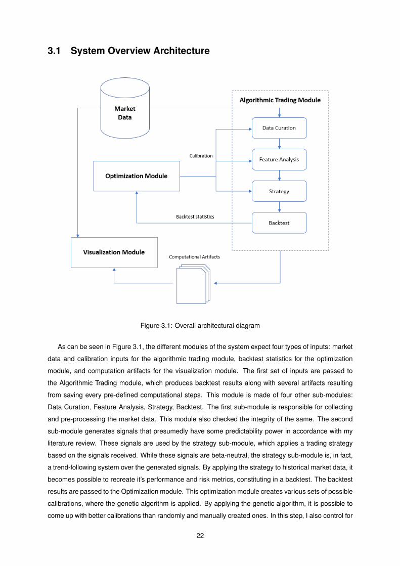
Figure 3.1: Overall architectural diagram
As can be seen in Figure 3.1, the different modules of the system expect four types of inputs: market
data and calibration inputs for the algorithmic trading module, backtest statistics for the optimization
module, and computation artifacts for the visualization module. The first set of inputs are passed to
the Algorithmic Trading module, which produces backtest results along with several artifacts resulting
from saving every pre-defined computational steps. This module is made of four other sub-modules:
Data Curation, Feature Analysis, Strategy, Backtest. The first sub-module is responsible for collecting
and pre-processing the market data. This module also checked the integrity of the same. The second
sub-module generates signals that presumedly have some predictability power in accordance with my
literature review. These signals are used by the strategy sub-module, which applies a trading strategy
based on the signals received. While these signals are beta-neutral, the strategy sub-module is, in fact,
a trend-following system over the generated signals. By applying the strategy to historical market data, it
becomes possible to recreate it’s performance and risk metrics, constituting in a backtest. The backtest
results are passed to the Optimization module. This optimization module creates various sets of possible
calibrations, where the genetic algorithm is applied. By applying the genetic algorithm, it is possible to
come up with better calibrations than randomly and manually created ones. In this step, I also control for
22
over-fitness of the generated calibrations by running them on validations sets. The Visualization module
can be used to present the various computational steps generated in past modules in a human-readable
manner. To do this, I use a python framework named Jupyter. This module is used to validate the
results, debug issues during the development of the application, and generate images and graphics that
are used in this work.
3.2 Algorithmic Trading Module
In this section, the most complex module in this work is explored. The algorithmic trading module is
composed of four different sub-modules that follow the work methodology presented by Prado [38]: Data
Curation, Feature Analysis, Strategy, and Backtesting. Each one of these sub-modules is individually
explored in subsequent chapters. Briefly, the algorithmic trading module works as follow:
1. For each pair of stocks, re-sample the historical market data and find common trading periods.
2. For each common trading period, generate a signal when one of the following verifies:
• The first stock of the pair doesn’t make a new high and the second one does.
• The first stock of the pair makes a new high and the second one doesn’t.
• The first stock of the pair doesn’t make a new low and the second one does.
• The first stock of the pair makes a new low and the second one doesn’t.
3. For each signal, a cointegration test is performed.
4. For each signal with a positive test, long the stock making new lows or short the stock making new
highs. Do the opposite for the other stock.
5. Generate an index with an hypothetical portfolio equally allocated across every signal.
6. Calculate slow and fast moving-averages over this index.
7. Replicate or inverse the index underlying trades based on a simple trend-following strategy.
3.2.1 Data Curation
The market data is fed to the Data Curation sub-module on a minute by minute basis, which is then
resampled into different intervals depending on the calibration that is provided. The minimum interval
for trading signals is on a daily scale. This module is capable of finding irregularities in the data, such
as substantial variations in very short periods of time and prevent using that instrument. This is done so
by highlighting and filtering out datapoints with unrealistic values. An unrealistic value is categorized as
a twenty percent change in values both before and after this datapoint within a one-minute period. The
curated data is exported to CSV files, which are reused to save computational resources in future runs.
The processed that is then instantiated as a list of vectors with information regarding the date, high, low,
open, and close of the instruments used. Since I am exploring the trading of pairs of equities, it is also in
this module where common trading intervals between the pairs are computed and saved. Trading pairs
23
also means that each instrument will be backtested with several other combinations of instruments; as
such, this list of vectors is cached in memory to reduce runtime duration significantly. This optimization
is later explained in chapter 3.6.
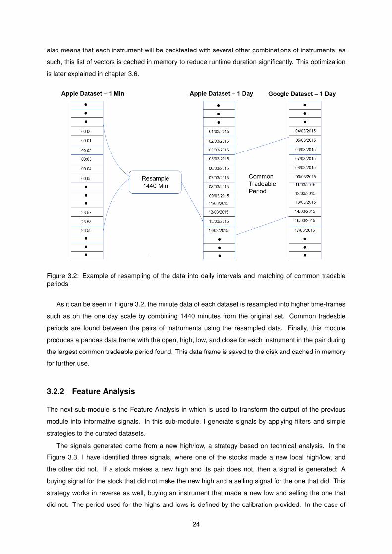
Figure 3.2: Example of resampling of the data into daily intervals and matching of common tradableperiods
As it can be seen in Figure 3.2, the minute data of each dataset is resampled into higher time-frames
such as on the one day scale by combining 1440 minutes from the original set. Common tradeable
periods are found between the pairs of instruments using the resampled data. Finally, this module
produces a pandas data frame with the open, high, low, and close for each instrument in the pair during
the largest common tradeable period found. This data frame is saved to the disk and cached in memory
for further use.
3.2.2 Feature Analysis
The next sub-module is the Feature Analysis in which is used to transform the output of the previous
module into informative signals. In this sub-module, I generate signals by applying filters and simple
strategies to the curated datasets.
The signals generated come from a new high/low, a strategy based on technical analysis. In the
Figure 3.3, I have identified three signals, where one of the stocks made a new local high/low, and
the other did not. If a stock makes a new high and its pair does not, then a signal is generated: A
buying signal for the stock that did not make the new high and a selling signal for the one that did. This
strategy works in reverse as well, buying an instrument that made a new low and selling the one that
did not. The period used for the highs and lows is defined by the calibration provided. In the case of
24
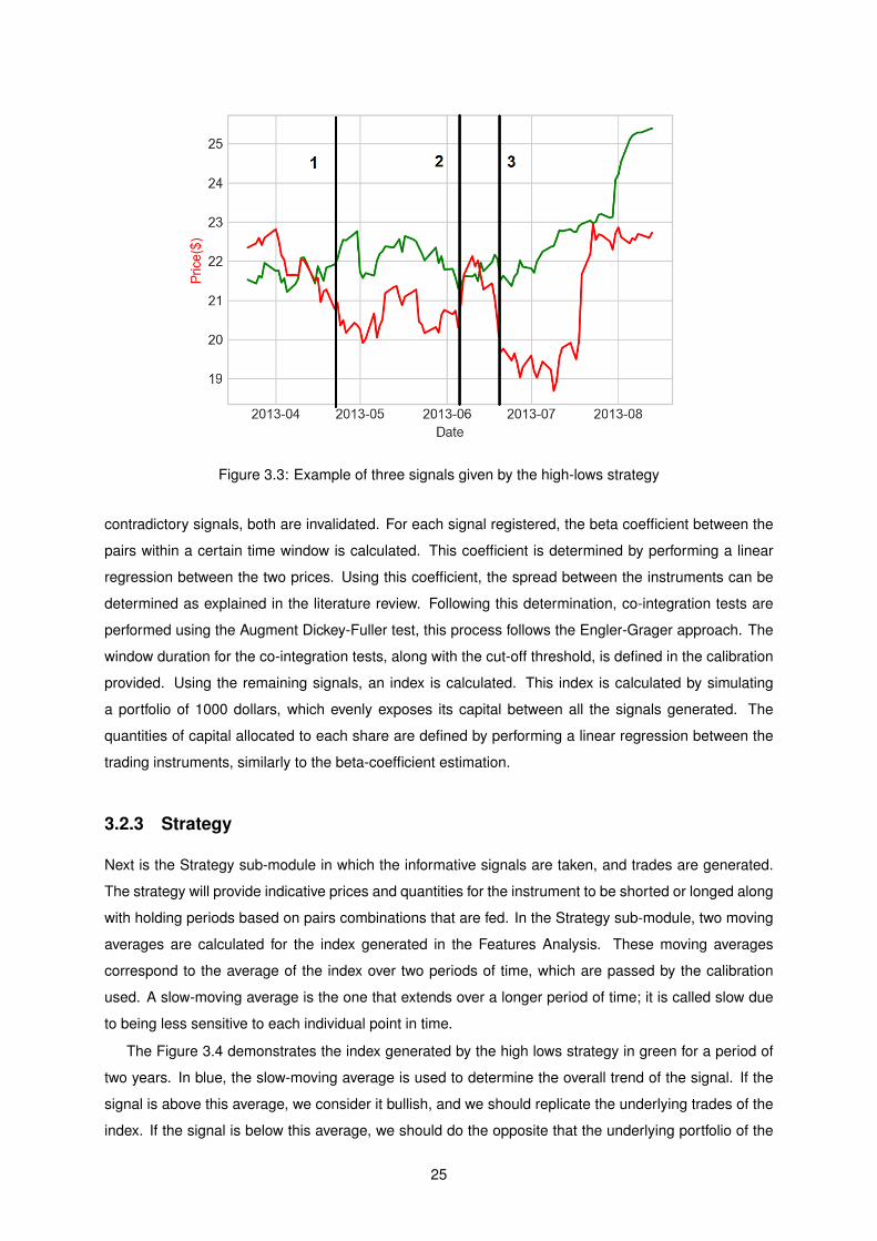
Figure 3.3: Example of three signals given by the high-lows strategy
contradictory signals, both are invalidated. For each signal registered, the beta coefficient between the
pairs within a certain time window is calculated. This coefficient is determined by performing a linear
regression between the two prices. Using this coefficient, the spread between the instruments can be
determined as explained in the literature review. Following this determination, co-integration tests are
performed using the Augment Dickey-Fuller test, this process follows the Engler-Grager approach. The
window duration for the co-integration tests, along with the cut-off threshold, is defined in the calibration
provided. Using the remaining signals, an index is calculated. This index is calculated by simulating
a portfolio of 1000 dollars, which evenly exposes its capital between all the signals generated. The
quantities of capital allocated to each share are defined by performing a linear regression between the
trading instruments, similarly to the beta-coefficient estimation.
3.2.3 Strategy
Next is the Strategy sub-module in which the informative signals are taken, and trades are generated.
The strategy will provide indicative prices and quantities for the instrument to be shorted or longed along
with holding periods based on pairs combinations that are fed. In the Strategy sub-module, two moving
averages are calculated for the index generated in the Features Analysis. These moving averages
correspond to the average of the index over two periods of time, which are passed by the calibration
used. A slow-moving average is the one that extends over a longer period of time; it is called slow due
to being less sensitive to each individual point in time.
The Figure 3.4 demonstrates the index generated by the high lows strategy in green for a period of
two years. In blue, the slow-moving average is used to determine the overall trend of the signal. If the
signal is above this average, we consider it bullish, and we should replicate the underlying trades of the
index. If the signal is below this average, we should do the opposite that the underlying portfolio of the
25
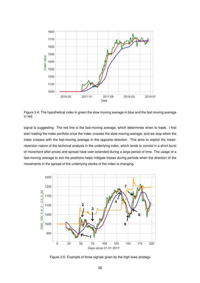
Figure 3.4: The hypothetical index in green the slow moving average in blue and the fast moving averagein red
signal is suggesting. The red line is the fast-moving average, which determines when to trade. I first
start trading the index portfolio once the index crosses the slow-moving average, and we stop when the
index crosses with the fast-moving average in the opposite direction. This aims to exploit the mean-
reversion nature of the technical analysis in the underlying index, which tends to consist in a short burst
of movement after prices and spread have over-extended during a large period of time. The usage of a
fast-moving average to exit the positions helps mitigate losses during periods when the direction of the
movements in the spread of the underlying stocks of the index is changing.
Figure 3.5: Example of three signals given by the high-lows strategy
26
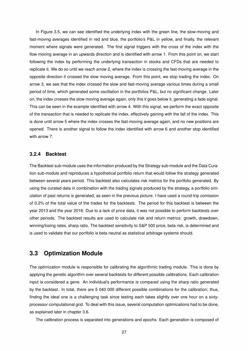
In Figure 3.5, we can see identified the underlying index with the green line, the slow-moving and
fast-moving averages identified in red and blue, the portfolio’s P&L in yellow, and finally, the relevant
moment where signals were generated. The first signal triggers with the cross of the index with the
flow moving average in an upwards direction and is identified with arrow 1. From this point on, we start
following the index by performing the underlying transaction in stocks and CFDs that are needed to
replicate it. We do so until we reach arrow 2, where the index is crossing the fast-moving average in the
opposite direction if crossed the slow moving average. From this point, we stop trading the index. On
arrow 3, we see that the index crossed the slow and fast-moving average various times during a small
period of time, which generated some oscillation in the portfolios P&L, but no significant change. Later
on, the index crosses the slow moving average again, only this it goes below it, generating a fade signal.
This can be seen in the example identified with arrow 4. With this signal, we perform the exact opposite
of the transaction that is needed to replicate the index, effectively gaining with the fall of the index. This
is done until arrow 5 where the index crosses the fast-moving average again, and no new positions are
opened. There is another signal to follow the index identified with arrow 6 and another stop identified
with arrow 7.
3.2.4 Backtest
The Backtest sub-module uses the information produced by the Strategy sub-module and the Data Cura-
tion sub-module and reproduces a hypothetical portfolio return that would follow the strategy generated
between several years period. This backtest also calculates risk metrics for the portfolio generated. By
using the curated data in combination with the trading signals produced by the strategy, a portfolio sim-
ulation of past returns is generated, as seen in the previous picture. I have used a round-trip comission
of 0.2% of the total value of the trades for the backtests. The period for this backtest is between the
year 2013 and the year 2018. Due to a lack of price data, it was not possible to perform backtests over
other periods. The backtest results are used to calculate risk and return metrics: growth, drawdown,
winning/losing rates, sharp ratio. The backtest sensitivity to S&P 500 price, beta risk, is determined and
is used to validate that our portfolio is beta neutral as statistical arbitrage systems should.
3.3 Optimization Module
The optimization module is responsible for calibrating the algorithmic trading module. This is done by
applying the genetic algorithm over several backtests for different possible calibrations. Each calibration
input is considered a gene. An individual’s performance is compared using the sharp ratio generated
by the backtest. In total, there are 5 040 000 different possible combinations for the calibration; thus,
finding the ideal one is a challenging task since testing each takes slightly over one hour on a sixty-
processor computational grid. To deal with this issue, several computation optimizations had to be done,
as explained later in chapter 3.6.
The calibration process is separated into generations and epochs. Each generation is composed of
27
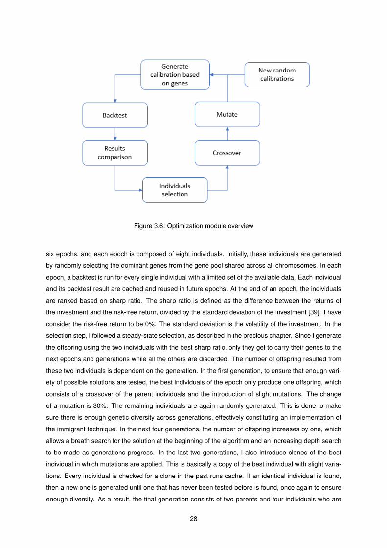
Figure 3.6: Optimization module overview
six epochs, and each epoch is composed of eight individuals. Initially, these individuals are generated
by randomly selecting the dominant genes from the gene pool shared across all chromosomes. In each
epoch, a backtest is run for every single individual with a limited set of the available data. Each individual
and its backtest result are cached and reused in future epochs. At the end of an epoch, the individuals
are ranked based on sharp ratio. The sharp ratio is defined as the difference between the returns of
the investment and the risk-free return, divided by the standard deviation of the investment [39]. I have
consider the risk-free return to be 0%. The standard deviation is the volatility of the investment. In the
selection step, I followed a steady-state selection, as described in the precious chapter. Since I generate
the offspring using the two individuals with the best sharp ratio, only they get to carry their genes to the
next epochs and generations while all the others are discarded. The number of offspring resulted from
these two individuals is dependent on the generation. In the first generation, to ensure that enough vari-
ety of possible solutions are tested, the best individuals of the epoch only produce one offspring, which
consists of a crossover of the parent individuals and the introduction of slight mutations. The change
of a mutation is 30%. The remaining individuals are again randomly generated. This is done to make
sure there is enough genetic diversity across generations, effectively constituting an implementation of
the immigrant technique. In the next four generations, the number of offspring increases by one, which
allows a breath search for the solution at the beginning of the algorithm and an increasing depth search
to be made as generations progress. In the last two generations, I also introduce clones of the best
individual in which mutations are applied. This is basically a copy of the best individual with slight varia-
tions. Every individual is checked for a clone in the past runs cache. If an identical individual is found,
then a new one is generated until one that has never been tested before is found, once again to ensure
enough diversity. As a result, the final generation consists of two parents and four individuals who are
28
their offspring and two individuals who are mutated clones from the best individual. We can see this
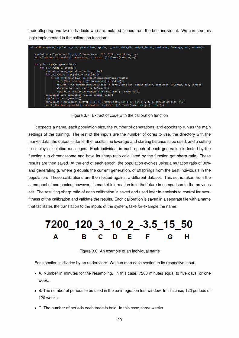
logic implemented in the calibration function:
Figure 3.7: Extract of code with the calibration function
It expects a name, each population size, the number of generations, and epochs to run as the main
settings of the training. The rest of the inputs are the number of cores to use, the directory with the
market data, the output folder for the results, the leverage and starting balance to be used, and a setting
to display calculation messages. Each individual in each epoch of each generation is tested by the
function run chromossome and have its sharp ratio calculated by the function get sharp ratio. These
results are then saved. At the end of each epoch, the population evolves using a mutation ratio of 30%
and generating g, where g equals the current generation, of offsprings from the best individuals in the
population. These calibrations are then tested against a different dataset. This set is taken from the
same pool of companies, however, its market information is in the future in comparison to the previous
set. The resulting sharp ratio of each calibration is saved and used later in analysis to control for over-
fitness of the calibration and validate the results. Each calibration is saved in a separate file with a name
that facilitates the translation to the inputs of the system, take for example the name:
Figure 3.8: An example of an individual name
Each section is divided by an underscore. We can map each section to its respective input:
• A. Number in minutes for the resampling. In this case, 7200 minutes equal to five days, or one
week.
• B. The number of periods to be used in the co-integration test window. In this case, 120 periods or
120 weeks.
• C. The number of periods each trade is held. In this case, three weeks.
29
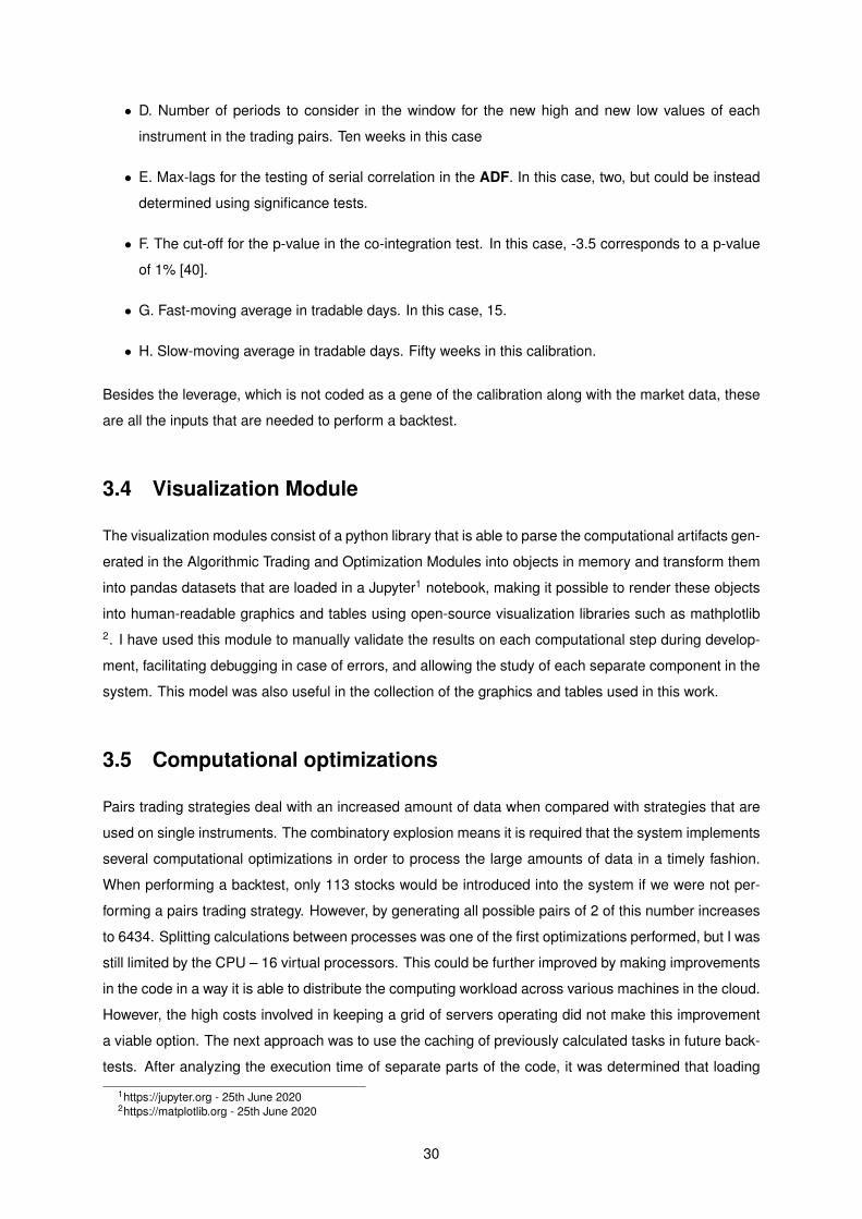
• D. Number of periods to consider in the window for the new high and new low values of each
instrument in the trading pairs. Ten weeks in this case
• E. Max-lags for the testing of serial correlation in the ADF. In this case, two, but could be instead
determined using significance tests.
• F. The cut-off for the p-value in the co-integration test. In this case, -3.5 corresponds to a p-value
of 1% [40].
• G. Fast-moving average in tradable days. In this case, 15.
• H. Slow-moving average in tradable days. Fifty weeks in this calibration.
Besides the leverage, which is not coded as a gene of the calibration along with the market data, these
are all the inputs that are needed to perform a backtest.
3.4 Visualization Module
The visualization modules consist of a python library that is able to parse the computational artifacts gen-
erated in the Algorithmic Trading and Optimization Modules into objects in memory and transform them
into pandas datasets that are loaded in a Jupyter1 notebook, making it possible to render these objects
into human-readable graphics and tables using open-source visualization libraries such as mathplotlib2. I have used this module to manually validate the results on each computational step during develop-
ment, facilitating debugging in case of errors, and allowing the study of each separate component in the
system. This model was also useful in the collection of the graphics and tables used in this work.
3.5 Computational optimizations
Pairs trading strategies deal with an increased amount of data when compared with strategies that are
used on single instruments. The combinatory explosion means it is required that the system implements
several computational optimizations in order to process the large amounts of data in a timely fashion.
When performing a backtest, only 113 stocks would be introduced into the system if we were not per-
forming a pairs trading strategy. However, by generating all possible pairs of 2 of this number increases
to 6434. Splitting calculations between processes was one of the first optimizations performed, but I was
still limited by the CPU – 16 virtual processors. This could be further improved by making improvements
in the code in a way it is able to distribute the computing workload across various machines in the cloud.
However, the high costs involved in keeping a grid of servers operating did not make this improvement
a viable option. The next approach was to use the caching of previously calculated tasks in future back-
tests. After analyzing the execution time of separate parts of the code, it was determined that loading
1https://jupyter.org - 25th June 20202https://matplotlib.org - 25th June 2020
30
and resampling the market data was consuming about half of each backtest. I have optimized the sys-
tem by keeping in RAM the market data of each individual stock in different sampling rates. Caching
the market data provided a significant improvement of about 7-10 seconds on each backtest (average
duration was 16-18 seconds). To be able to run the calibration uninterruptedly, I have configured a
cloud web server to run the optimization module and later secure copied the results. Since I had to test
different providers, I have created shell scripts that automatically perform the configuration for Ubuntu
18.0 servers to be able to run the proposed system. Finally, to ensure reproducibility and as a safety
mechanism for events that might disrupt or interrupt the calibration, there are several checkpoints where
objects that resulted from lengthy computations are exported and written in the disk along with the logs
of the application. In case of failure, when resuming the calibration process, the existence of already
previously calculated objects is checked before performing computationally intensive parts and loaded
into memory.
3.6 Data Used
The system developed in combination with this work, requires market data to function. The market data
that was used in the experiments mentioned in the next chapter consist of minute-base stock information
from interactive brokers along with CFD data on three indexes: Standard and Poor 500, which is a
market-capitalization-weighted index based on the largest 500 publicly traded USA companies; Dow 30,
similar to the previous index but only takes in 30 companies; and finally, the Nasdaq 100 yet another
similar index that however focuses on technology companies and excludes other industries with the
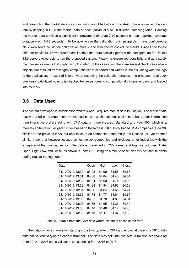
exception of the financial sector. The data is presented in CSV format and has five columns: Date,
Open, High, Low, and Close, as shown in Table 3.1. Being on a minute base, an entry per minute exists
during regular trading hours.
Date Open High Low Close
31/10/2012 13:30 84.93 84.99 84.58 84.6531/10/2012 13:31 84.68 84.84 84.45 84.8431/10/2012 13:32 84.84 85.00 84.74 84.9031/10/2012 13:33 84.88 84.94 84.65 84.6531/10/2012 13:34 84.66 84.84 84.65 84.7431/10/2012 13:35 84.73 84.77 84.61 84.6731/10/2012 13:36 84.67 84.76 84.60 84.6431/10/2012 13:37 84.65 84.65 84.36 84.4031/10/2012 13:38 84.40 84.48 84.17 84.4831/10/2012 13:39 84.45 84.47 84.37 84.39
Table 3.1: Table from the CSV data where historical prices come from
The data contains information starting in the third quarter of 2012 and ending at the end of 2018, with
different periods varying on each instrument. The data was split into two sets, a training set spanning
from 2012 to 2016 and a validation set spanning from 2016 to 2018.
31

32

Chapter 4
Studies and Validation
In this chapter, I describe, perform, and analyze three different studies from which I take the main
contributions of this work. Each study is divided into four sections: hypothesis, experiments, results, and
limitations. In the hypothesis section, I describe what problem questions I am interested in exploring,
along with the various possible answers there might be and how they could be tested and validated. In
the experiments section, I design the experiments that will attempt to answer the problem questions and
validate the hypothesis described in the previous section. I describe the experiments, how they were
conducted, validated, and I extract the results. In the results section, I analyze the collected results,
and based on that, I extract conclusions and answer the problem questions under study. This is also
where the results are validated, and contributions extracted. In the limitations section, I explore the
limitations of my experiments and the collected conclusions. The first study aims at exploring the usage
of artificial intelligence techniques to optimize statistical arbitrage strategies. The second study explores
the usage of co-integration as a way to find tradable pairs of stocks. Finally, the third study compares the
performance of the system developed in Chapter 3 against similar systems and how this system could
be deployed in a real-world environment.
33
4.1 Study 1 – Calibration efficiency
In this first study, I explored the main problem-question: if it is possible to use AI to optimize a simple
statistical arbitrage strategy. I use the strategy described in the previous chapter and collect its backtest
performance using random calibrations. I then attempt to optimize the calibrations using the optimization
module and compare the results against several risk metrics. The main contribution of this study is how
it tests the efficiency of the optimization module described in section 3.4 of this work: the assemble of a
genetic algorithm that backtests possible sets of inputs and to generate optimized results.
4.1.1 Hypothesis
The main problem question I am tackling in this section is if it is possible to use artificial intelligence
techniques to optimize a statistical arbitrage strategy. As such, this statement should hold as truth if I
can find and measure the results of a statistical arbitrage strategy and if later, I can generate improved
results by optimizing some part of the statistical arbitrage strategy, or it’s whole. I believe this is possible
since, as seen on the literature review in Chapter 2, some authors such as Linn and Hulk have developed
entire statistical arbitrage strategies and systems having artificial intelligence techniques such as Elman
networks and Principle Component Analysis Prado also describes in his book various techniques in
which artificial intelligence was used to optimize trading strategies. If I am able to generate improved
backtest results by calibrating the system using the genetic algorithm, then I can conclude it is possible
to use artificial intelligence techniques to optimize these types of strategies. However, if I am not able to
determine with confidence that the results have been improved due to the usage of the genetic algorithm,
or if the results are not improved by the usage of the genetic algorithm, then the hypothesis remains open
as it is still possible that there are other systems or other artificial intelligence optimization techniques
that could be used to improve the results.
4.1.2 Experiments
In order to test the hypothesis, I have used the system designed in Chapter 3. I began by generating
random calibrations for the system within a range of parameters where these calibrations would still
make sense (for example, the slow-moving average could not be faster than the fast-moving average).
Next, I have separated the available market data into two sets: a test set and a validation set. I have then
performed backtests over the validation set for each of the randomly generated calibrations and collected
the results. Since the optimization module uses the genetic algorithm to find better calibrations, if I can
find a better calibration using this optimization module, then I can validate the hypothesis under study.
As such, I have proceeded to feed the randomly generated configurations as the first population of the
optimization module. I have run the algorithm for eight generations with six epochs each. Each epoch
had eight individuals. Instead of using the validation set, the optimization applied the genetic algorithm
over these individuals using the market data in the test set. This is done in order to not bias the training
towards the same set of data from where I will extract the performance. Having this separation also
34
allows me to check for over-fitness of the training. Once the results from the training are collected, I
have proceeded to backtest all calibrations generated by the genetic algorithm against the validation
set and proceeded to save the results. Since the system uses information up to 200 weeks prior to the
current day to generate the signals and perform co-integration tests, the historical data in the validation
set also contains data from the training set. However, no trades are performed under the same period.
As such, the data from the training set in the validation set is only used to calculate indicator data in the
feature analysis sub-module of the algorithmic trading module.
Figure 4.1: Training and Validation sets
The Figure 4.1 shows the data that is used to generate the trading signals and the separation be-
tween the training, letters A and B, and validation set, letters C and D. Each set is broken and categorized
into two other sets, indicator calculation, letters A and C, and trading set, letters B and D. The optimiza-
tion module feeds on data that spans from the beginning of the set in 2014 until a cut-off in late 2016 to
find the best calibrations. The results are validated against the data that spans from mid-2016 until the
end of the set in 2018, identified by the letters C and D. Therefore, there is one year of data where both
sets are overlapping, which happens due to C being partially contained in B. While the co-integration
tests and indicator data use information from the past days that are used in the training set, it should be
noted that the core trigger for a trade signal generation does not have information contained in this pre-
vious set. This is because the trigger is given by the technical analysis/arbitrage signal resulting from a
break of a local support or resistance in one of the pairs being watched, and the overlapping only exists
during indicator calculation of the validation set: There is no overlapping between the trading periods.
Finally, I have used the results generated by the backtest to collect other significant portfolio measures
such as win/loss ratio, average win, loss, drawdown, and beta coefficient against the general market and
plotted these using the visualization module. The objective of this step is to validate that the portfolios
resulting from the backtest are still beta-neutral in relation to the S&P 500.
35
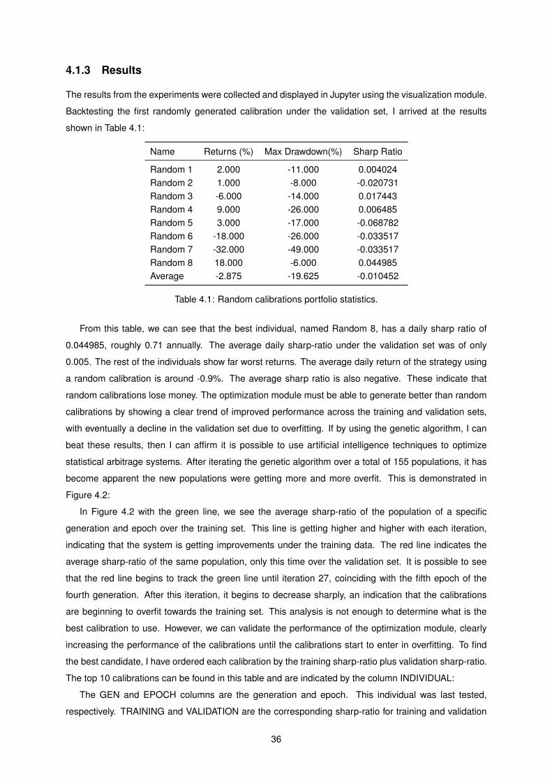
4.1.3 Results
The results from the experiments were collected and displayed in Jupyter using the visualization module.
Backtesting the first randomly generated calibration under the validation set, I arrived at the results
shown in Table 4.1:
Name Returns (%) Max Drawdown(%) Sharp Ratio
Random 1 2.000 -11.000 0.004024Random 2 1.000 -8.000 -0.020731Random 3 -6.000 -14.000 0.017443Random 4 9.000 -26.000 0.006485Random 5 3.000 -17.000 -0.068782Random 6 -18.000 -26.000 -0.033517Random 7 -32.000 -49.000 -0.033517Random 8 18.000 -6.000 0.044985Average -2.875 -19.625 -0.010452
Table 4.1: Random calibrations portfolio statistics.
From this table, we can see that the best individual, named Random 8, has a daily sharp ratio of
0.044985, roughly 0.71 annually. The average daily sharp-ratio under the validation set was of only
0.005. The rest of the individuals show far worst returns. The average daily return of the strategy using
a random calibration is around -0.9%. The average sharp ratio is also negative. These indicate that
random calibrations lose money. The optimization module must be able to generate better than random
calibrations by showing a clear trend of improved performance across the training and validation sets,
with eventually a decline in the validation set due to overfitting. If by using the genetic algorithm, I can
beat these results, then I can affirm it is possible to use artificial intelligence techniques to optimize
statistical arbitrage systems. After iterating the genetic algorithm over a total of 155 populations, it has
become apparent the new populations were getting more and more overfit. This is demonstrated in
Figure 4.2:
In Figure 4.2 with the green line, we see the average sharp-ratio of the population of a specific
generation and epoch over the training set. This line is getting higher and higher with each iteration,
indicating that the system is getting improvements under the training data. The red line indicates the
average sharp-ratio of the same population, only this time over the validation set. It is possible to see
that the red line begins to track the green line until iteration 27, coinciding with the fifth epoch of the
fourth generation. After this iteration, it begins to decrease sharply, an indication that the calibrations
are beginning to overfit towards the training set. This analysis is not enough to determine what is the
best calibration to use. However, we can validate the performance of the optimization module, clearly
increasing the performance of the calibrations until the calibrations start to enter in overfitting. To find
the best candidate, I have ordered each calibration by the training sharp-ratio plus validation sharp-ratio.
The top 10 calibrations can be found in this table and are indicated by the column INDIVIDUAL:
The GEN and EPOCH columns are the generation and epoch. This individual was last tested,
respectively. TRAINING and VALIDATION are the corresponding sharp-ratio for training and validation
36
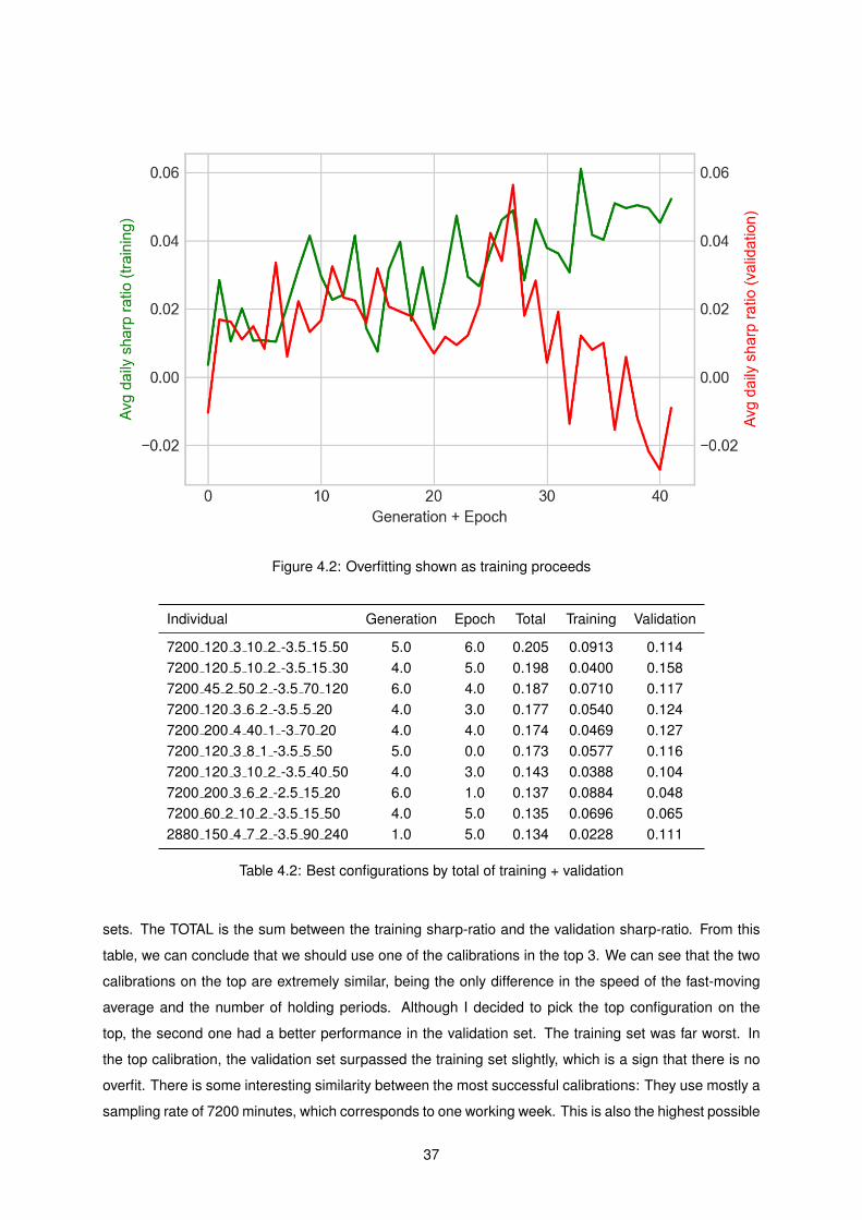
Figure 4.2: Overfitting shown as training proceeds
Individual Generation Epoch Total Training Validation
7200 120 3 10 2 -3.5 15 50 5.0 6.0 0.205 0.0913 0.1147200 120 5 10 2 -3.5 15 30 4.0 5.0 0.198 0.0400 0.1587200 45 2 50 2 -3.5 70 120 6.0 4.0 0.187 0.0710 0.1177200 120 3 6 2 -3.5 5 20 4.0 3.0 0.177 0.0540 0.1247200 200 4 40 1 -3 70 20 4.0 4.0 0.174 0.0469 0.1277200 120 3 8 1 -3.5 5 50 5.0 0.0 0.173 0.0577 0.1167200 120 3 10 2 -3.5 40 50 4.0 3.0 0.143 0.0388 0.1047200 200 3 6 2 -2.5 15 20 6.0 1.0 0.137 0.0884 0.0487200 60 2 10 2 -3.5 15 50 4.0 5.0 0.135 0.0696 0.0652880 150 4 7 2 -3.5 90 240 1.0 5.0 0.134 0.0228 0.111
Table 4.2: Best configurations by total of training + validation
sets. The TOTAL is the sum between the training sharp-ratio and the validation sharp-ratio. From this
table, we can conclude that we should use one of the calibrations in the top 3. We can see that the two
calibrations on the top are extremely similar, being the only difference in the speed of the fast-moving
average and the number of holding periods. Although I decided to pick the top configuration on the
top, the second one had a better performance in the validation set. The training set was far worst. In
the top calibration, the validation set surpassed the training set slightly, which is a sign that there is no
overfit. There is some interesting similarity between the most successful calibrations: They use mostly a
sampling rate of 7200 minutes, which corresponds to one working week. This is also the highest possible
37
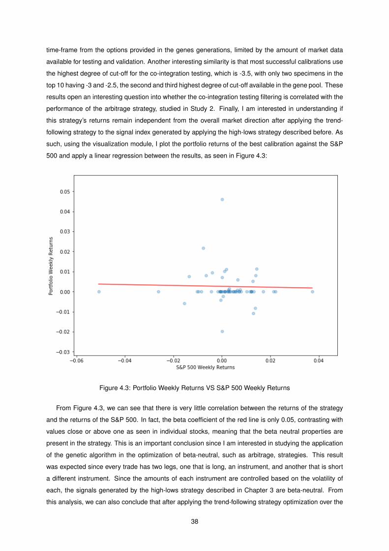
time-frame from the options provided in the genes generations, limited by the amount of market data
available for testing and validation. Another interesting similarity is that most successful calibrations use
the highest degree of cut-off for the co-integration testing, which is -3.5, with only two specimens in the
top 10 having -3 and -2.5, the second and third highest degree of cut-off available in the gene pool. These
results open an interesting question into whether the co-integration testing filtering is correlated with the
performance of the arbitrage strategy, studied in Study 2. Finally, I am interested in understanding if
this strategy’s returns remain independent from the overall market direction after applying the trend-
following strategy to the signal index generated by applying the high-lows strategy described before. As
such, using the visualization module, I plot the portfolio returns of the best calibration against the S&P
500 and apply a linear regression between the results, as seen in Figure 4.3:
Figure 4.3: Portfolio Weekly Returns VS S&P 500 Weekly Returns
From Figure 4.3, we can see that there is very little correlation between the returns of the strategy
and the returns of the S&P 500. In fact, the beta coefficient of the red line is only 0.05, contrasting with
values close or above one as seen in individual stocks, meaning that the beta neutral properties are
present in the strategy. This is an important conclusion since I am interested in studying the application
of the genetic algorithm in the optimization of beta-neutral, such as arbitrage, strategies. This result
was expected since every trade has two legs, one that is long, an instrument, and another that is short
a different instrument. Since the amounts of each instrument are controlled based on the volatility of
each, the signals generated by the high-lows strategy described in Chapter 3 are beta-neutral. From
this analysis, we can also conclude that after applying the trend-following strategy optimization over the
38
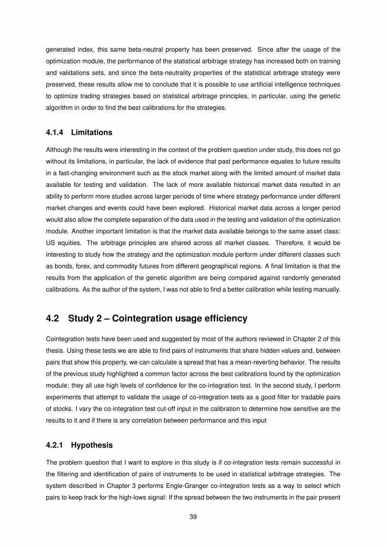
generated index, this same beta-neutral property has been preserved. Since after the usage of the
optimization module, the performance of the statistical arbitrage strategy has increased both on training
and validations sets, and since the beta-neutrality properties of the statistical arbitrage strategy were
preserved, these results allow me to conclude that it is possible to use artificial intelligence techniques
to optimize trading strategies based on statistical arbitrage principles, in particular, using the genetic
algorithm in order to find the best calibrations for the strategies.
4.1.4 Limitations
Although the results were interesting in the context of the problem question under study, this does not go
without its limitations, in particular, the lack of evidence that past performance equates to future results
in a fast-changing environment such as the stock market along with the limited amount of market data
available for testing and validation. The lack of more available historical market data resulted in an
ability to perform more studies across larger periods of time where strategy performance under different
market changes and events could have been explored. Historical market data across a longer period
would also allow the complete separation of the data used in the testing and validation of the optimization
module. Another important limitation is that the market data available belongs to the same asset class:
US equities. The arbitrage principles are shared across all market classes. Therefore, it would be
interesting to study how the strategy and the optimization module perform under different classes such
as bonds, forex, and commodity futures from different geographical regions. A final limitation is that the
results from the application of the genetic algorithm are being compared against randomly generated
calibrations. As the author of the system, I was not able to find a better calibration while testing manually.
4.2 Study 2 – Cointegration usage efficiency
Cointegration tests have been used and suggested by most of the authors reviewed in Chapter 2 of this
thesis. Using these tests we are able to find pairs of instruments that share hidden values and, between
pairs that show this property, we can calculate a spread that has a mean-reverting behavior. The results
of the previous study highlighted a common factor across the best calibrations found by the optimization
module: they all use high levels of confidence for the co-integration test. In the second study, I perform
experiments that attempt to validate the usage of co-integration tests as a good filter for tradable pairs
of stocks. I vary the co-integration test cut-off input in the calibration to determine how sensitive are the
results to it and if there is any correlation between performance and this input
4.2.1 Hypothesis
The problem question that I want to explore in this study is if co-integration tests remain successful in
the filtering and identification of pairs of instruments to be used in statistical arbitrage strategies. The
system described in Chapter 3 performs Engle-Granger co-integration tests as a way to select which
pairs to keep track for the high-lows signal: If the spread between the two instruments in the pair present
39
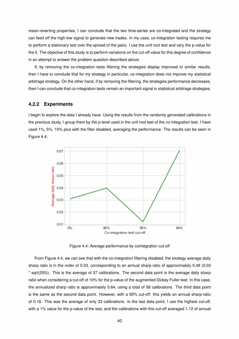
mean-reverting properties, I can conclude that the two time-series are co-integrated and the strategy
can feed off the high-low signal to generate new trades. In my case, co-integration testing requires me
to perform a stationary test over the spread of the pairs. I use the unit root test and vary the p-value for
the it. The objective of this study is to perform variations on the cut-off value for this degree of confidence
in an attempt to answer the problem question described above.
If, by removing the co-integration tests filtering the strategies display improved or similar results,
then I have to conclude that for my strategy in particular, co-integration does not improve my statistical
arbitrage strategy. On the other hand, if by removing the filtering, the strategies performance decreases,
then I can conclude that co-integration tests remain an important signal in statistical arbitrage strategies.
4.2.2 Experiments
I begin to explore the data I already have. Using the results from the randomly generated calibrations in
the previous study, I group them by the p-level used in the unit root test of the co-integration test. I have
used 1%, 5%, 10% plus with the filter disabled, averaging the performance. The results can be seen in
Figure 4.4:
Figure 4.4: Average performance by cointegration cut-off
From Figure 4.4, we can see that with the co-integration filtering disabled, the strategy average daily
sharp ratio is in the order of 0.03, corresponding to an annual sharp-ratio of approximately 0.48 (0.03
* sqrt(255)). This is the average of 37 calibrations. The second data point is the average daily sharp
ratio when considering a cut-off of 10% for the p-value of the augmented Dickey-Fuller test. In this case,
the annualized sharp ratio is approximately 0.64, using a total of 58 calibrations. The third data point
is the same as the second data point. However, with a 95% cut-off: this yields an annual sharp-ratio
of 0.18. This was the average of only 33 calibrations. In the last data point, I use the highest cut-off,
with a 1% value for the p-value of the test, and the calibrations with this cut-off averaged 1.12 of annual
40
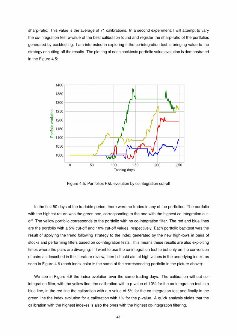
sharp-ratio. This value is the average of 71 calibrations. In a second experiment, I will attempt to vary
the co-integration test p-value of the best calibration found and register the sharp-ratio of the portfolios
generated by backtesting. I am interested in exploring if the co-integration test is bringing value to the
strategy or cutting-off the results. The plotting of each backtests portfolio value evolution is demonstrated
in the Figure 4.5:
Figure 4.5: Portfolios P&L evolution by cointegration cut-off
In the first 50 days of the tradable period, there were no trades in any of the portfolios. The portfolio
with the highest return was the green one, corresponding to the one with the highest co-integration cut-
off. The yellow portfolio corresponds to the portfolio with no co-integration filter. The red and blue lines
are the portfolio with a 5% cut-off and 10% cut-off values, respectively. Each portfolio backtest was the
result of applying the trend following strategy to the index generated by the new high-lows in pairs of
stocks and performing filters based on co-integration tests. This means these results are also exploiting
times where the pairs are diverging. If I want to use the co-integration test to bet only on the conversion
of pairs as described in the literature review, then I should aim at high values in the underlying index, as
seen in Figure 4.6 (each index color is the same of the corresponding portfolio in the picture above):
We see in Figure 4.6 the index evolution over the same trading days. The calibration without co-
integration filter, with the yellow line, the calibration with a p-value of 10% for the co-integration test in a
blue line, in the red line the calibration with a p-value of 5% for the co-integration test and finally in the
green line the index evolution for a calibration with 1% for the p-value. A quick analysis yields that the
calibration with the highest indexes is also the ones with the highest co-integration filtering.
41
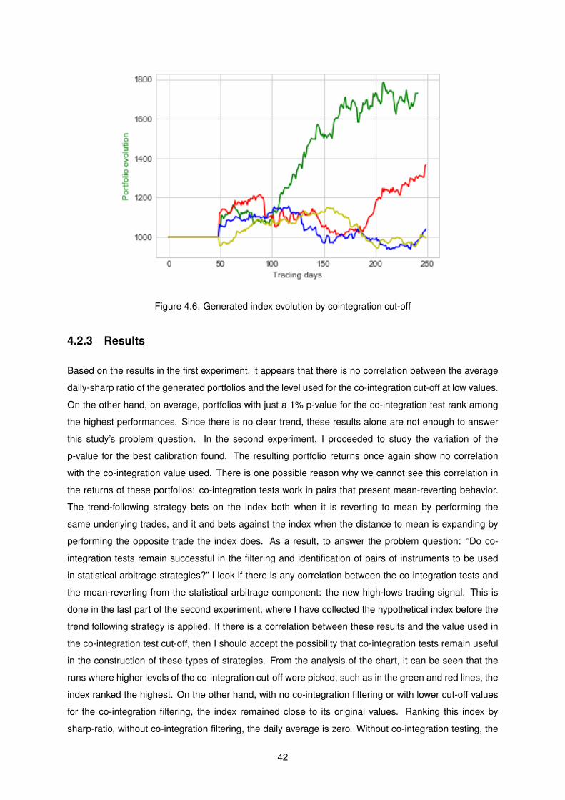
Figure 4.6: Generated index evolution by cointegration cut-off
4.2.3 Results
Based on the results in the first experiment, it appears that there is no correlation between the average
daily-sharp ratio of the generated portfolios and the level used for the co-integration cut-off at low values.
On the other hand, on average, portfolios with just a 1% p-value for the co-integration test rank among
the highest performances. Since there is no clear trend, these results alone are not enough to answer
this study’s problem question. In the second experiment, I proceeded to study the variation of the
p-value for the best calibration found. The resulting portfolio returns once again show no correlation
with the co-integration value used. There is one possible reason why we cannot see this correlation in
the returns of these portfolios: co-integration tests work in pairs that present mean-reverting behavior.
The trend-following strategy bets on the index both when it is reverting to mean by performing the
same underlying trades, and it and bets against the index when the distance to mean is expanding by
performing the opposite trade the index does. As a result, to answer the problem question: ”Do co-
integration tests remain successful in the filtering and identification of pairs of instruments to be used
in statistical arbitrage strategies?” I look if there is any correlation between the co-integration tests and
the mean-reverting from the statistical arbitrage component: the new high-lows trading signal. This is
done in the last part of the second experiment, where I have collected the hypothetical index before the
trend following strategy is applied. If there is a correlation between these results and the value used in
the co-integration test cut-off, then I should accept the possibility that co-integration tests remain useful
in the construction of these types of strategies. From the analysis of the chart, it can be seen that the
runs where higher levels of the co-integration cut-off were picked, such as in the green and red lines, the
index ranked the highest. On the other hand, with no co-integration filtering or with lower cut-off values
for the co-integration filtering, the index remained close to its original values. Ranking this index by
sharp-ratio, without co-integration filtering, the daily average is zero. Without co-integration testing, the
42
strategy returns a signal that looks like just noise. On the other hand, as I decrease the p-value in the co-
integration tests, the sharp-ratio increases to 0.02, 0.09, and 0.17 for respectively a p-value of 10%, 5%,
and 1%. As a result, I conclude that co-integration tests remain a useful signal to detect mean-reverting
behavior in the spread of pairs of stocks used in, for example, statistical arbitrage strategies.
4.2.4 Limitations
The conclusions of this study do not come out without its limitations. Similarly to the first study, there
is a lack of more historical trading data, both across different dates, geographical locations, and asset
classes. In the context of this study, this first limitation means that the instruments used in the pairs of
the statistical arbitrage strategy were both all from the same asset class (stocks, with the exception of
the three indexes) and from the same geographical location (USA), which means that there were already
some variables shared across these. With a more diverse dataset, the difference between the usage
of co-integration filters could be accentuated. Another limitation is the lack of backtests in the second
experiment, due to the lack of available resources for more backtesting, and the fact that this analysis is
limited to a single statistical arbitrage strategy. These limitations can be explored in further work.
4.3 Study 3 – Strategy comparison against similar portfolios
When assessing and comparing a track record to take an investment decision, portfolio managers look
at how the investment performance compares against the general market often using the S&P 500 as
the benchmark, and explore risk metrics such as drawdown, returns, and average trade performance. In
the third study, I compare this strategy performance against similar strategies and compare the strategy
performance of the best calibration found in the first study against the S&P 500 both before and after
adjusting the leverage to match the same levels of drawdown. I also review how this strategy could be
deployed and what limitations it might have.
4.3.1 Hypothesis
A portfolio manager survives off fees on the returns of the assets he is managing. The portfolio man-
ager costumers are only interested in his services if he is capable of generating enough returns to
compensate for the fees within the costumer’s risk profile and other available investments. Due to the
high variation of fees between funds, I won’t have them in consideration in this analysis. In this study,
I want to answer the problem question: Would a finance professional, or portfolio manager, invest in a
portfolio following the strategy in Chapter 3 using the best calibration found in the first study? To do this,
I will compare the portfolio performance against similar strategies and against the S&P 500 index. If my
portfolio performance during the validation period in the backtest has better results, within similar risk
profiles than the other options available, then I will conclude that the finance professional should invest
in the strategy described in this thesis. If instead, the results of the portfolio are worst than the available
alternatives, then I need to conclude that it would not be in the interest of the investor to follow this
43
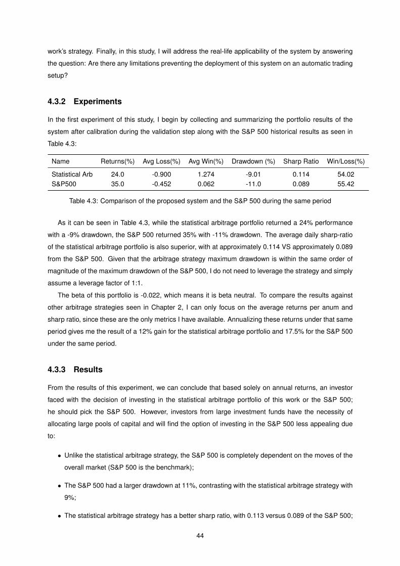
work’s strategy. Finally, in this study, I will address the real-life applicability of the system by answering
the question: Are there any limitations preventing the deployment of this system on an automatic trading
setup?
4.3.2 Experiments
In the first experiment of this study, I begin by collecting and summarizing the portfolio results of the
system after calibration during the validation step along with the S&P 500 historical results as seen in
Table 4.3:
Name Returns(%) Avg Loss(%) Avg Win(%) Drawdown (%) Sharp Ratio Win/Loss(%)
Statistical Arb 24.0 -0.900 1.274 -9.01 0.114 54.02S&P500 35.0 -0.452 0.062 -11.0 0.089 55.42
Table 4.3: Comparison of the proposed system and the S&P 500 during the same period
As it can be seen in Table 4.3, while the statistical arbitrage portfolio returned a 24% performance
with a -9% drawdown, the S&P 500 returned 35% with -11% drawdown. The average daily sharp-ratio
of the statistical arbitrage portfolio is also superior, with at approximately 0.114 VS approximately 0.089
from the S&P 500. Given that the arbitrage strategy maximum drawdown is within the same order of
magnitude of the maximum drawdown of the S&P 500, I do not need to leverage the strategy and simply
assume a leverage factor of 1:1.
The beta of this portfolio is -0.022, which means it is beta neutral. To compare the results against
other arbitrage strategies seen in Chapter 2, I can only focus on the average returns per anum and
sharp ratio, since these are the only metrics I have available. Annualizing these returns under that same
period gives me the result of a 12% gain for the statistical arbitrage portfolio and 17.5% for the S&P 500
under the same period.
4.3.3 Results
From the results of this experiment, we can conclude that based solely on annual returns, an investor
faced with the decision of investing in the statistical arbitrage portfolio of this work or the S&P 500;
he should pick the S&P 500. However, investors from large investment funds have the necessity of
allocating large pools of capital and will find the option of investing in the S&P 500 less appealing due
to:
• Unlike the statistical arbitrage strategy, the S&P 500 is completely dependent on the moves of the
overall market (S&P 500 is the benchmark);
• The S&P 500 had a larger drawdown at 11%, contrasting with the statistical arbitrage strategy with
9%;
• The statistical arbitrage strategy has a better sharp ratio, with 0.113 versus 0.089 of the S&P 500;
44
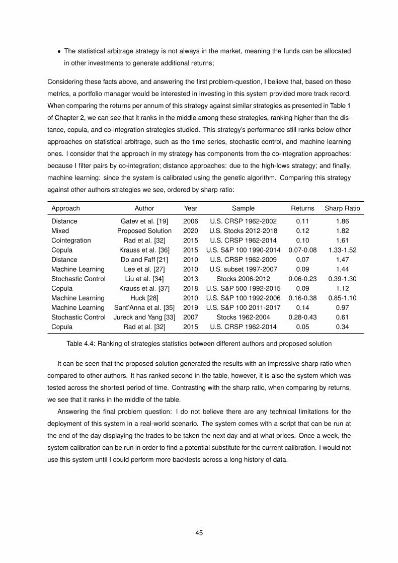
• The statistical arbitrage strategy is not always in the market, meaning the funds can be allocated
in other investments to generate additional returns;
Considering these facts above, and answering the first problem-question, I believe that, based on these
metrics, a portfolio manager would be interested in investing in this system provided more track record.
When comparing the returns per annum of this strategy against similar strategies as presented in Table 1
of Chapter 2, we can see that it ranks in the middle among these strategies, ranking higher than the dis-
tance, copula, and co-integration strategies studied. This strategy’s performance still ranks below other
approaches on statistical arbitrage, such as the time series, stochastic control, and machine learning
ones. I consider that the approach in my strategy has components from the co-integration approaches:
because I filter pairs by co-integration; distance approaches: due to the high-lows strategy; and finally,
machine learning: since the system is calibrated using the genetic algorithm. Comparing this strategy
against other authors strategies we see, ordered by sharp ratio:
Approach Author Year Sample Returns Sharp Ratio
Distance Gatev et al. [19] 2006 U.S. CRSP 1962-2002 0.11 1.86Mixed Proposed Solution 2020 U.S. Stocks 2012-2018 0.12 1.82Cointegration Rad et al. [32] 2015 U.S. CRSP 1962-2014 0.10 1.61Copula Krauss et al. [36] 2015 U.S. S&P 100 1990-2014 0.07-0.08 1.33-1.52Distance Do and Faff [21] 2010 U.S. CRSP 1962-2009 0.07 1.47Machine Learning Lee et al. [27] 2010 U.S. subset 1997-2007 0.09 1.44Stochastic Control Liu et al. [34] 2013 Stocks 2006-2012 0.06-0.23 0.39-1.30Copula Krauss et al. [37] 2018 U.S. S&P 500 1992-2015 0.09 1.12Machine Learning Huck [28] 2010 U.S. S&P 100 1992-2006 0.16-0.38 0.85-1.10Machine Learning Sant’Anna et al. [35] 2019 U.S. S&P 100 2011-2017 0.14 0.97Stochastic Control Jureck and Yang [33] 2007 Stocks 1962-2004 0.28-0.43 0.61Copula Rad et al. [32] 2015 U.S. CRSP 1962-2014 0.05 0.34
Table 4.4: Ranking of strategies statistics between different authors and proposed solution
It can be seen that the proposed solution generated the results with an impressive sharp ratio when
compared to other authors. It has ranked second in the table, however, it is also the system which was
tested across the shortest period of time. Contrasting with the sharp ratio, when comparing by returns,
we see that it ranks in the middle of the table.
Answering the final problem question: I do not believe there are any technical limitations for the
deployment of this system in a real-world scenario. The system comes with a script that can be run at
the end of the day displaying the trades to be taken the next day and at what prices. Once a week, the
system calibration can be run in order to find a potential substitute for the current calibration. I would not
use this system until I could perform more backtests across a long history of data.
45
4.3.4 Limitations
The main limitation of this study is the lack of historical data that would allow testing the performance
of the strategy across a larger variety of market conditions and events. This lack of historical data also
affects the comparisons made against the S&P 500, which had some of its best historical performance
during the period under study, averaging a return of 17.5% instead of a normal 10-12%.
This lack of data also affects the comparison against other arbitrage strategies: some of these strate-
gies returns are calculated based on the average returns of over forty years, such as the case in distance
approaches.
A final limitation is the lack of risk metrics for the other statistical arbitrage portfolios that were studied,
such as the drawdown and beta-coefficient against the S&P 500, which would allow me to compare
each portfolio’s performance against their volatility and adjust the leverage in my own system for a fair
comparison of returns.
46

Chapter 5
Conclusions
This chapter concludes the thesis. In it, I highlight the principal achievements and contributions of this
work for each of the studies and I make some recommendations of future work in this topic.
47

5.1 Achievements
From the results presented in my studies, it is possible to conclude that based on these, it is possible to
improve the statistical arbitrage trading strategy using machine learning techniques such as the genetic
algorithm. From the second study, it is possible to conclude co-integration tests remain an important
indicator to take into account when determining the pairs of stocks to trade a mean-reverting spread. The
third study concluded that this strategy fits the risk-profile of someone investing in most stock indexes;
however, for the periods under study, it produced smaller returns. From this study alone, it is not possible
to conclude how portfolios generated by this strategy react under different market conditions other than
the six-year period under study. It is technically possible to deploy this system in a real-world scenario.
Finally, the lack of evidence that past results do not equate to similar performance in the future, and
from the small number of years in the data from which the experiments were conducted, I would not
recommend deploying this strategy until more backtesting is done.
5.2 Future Work
For further work, I believe it would be interesting to explore:
• How is the performance of the portfolios generated by this system across longer periods of time;
• How is the performance affected by using different asset classes such as commodities and bonds;
• How does the performance vary depending on the usage of different co-integration tests;
• Perform calibrations using separate polls of genes for the different inputs in each sub-module;
• Attempt the usage of other machine learning techniques, such as the PCA, to perform a feature
reduction on the generated signals.
48
Bibliography
[1] B. J. and D. P. Corporate Finance, page 995. Springer, 2013.
[2] A. W. Lo. What is an index? The Journal of Portfolio Management, 2016.
[3] B. J. and D. P. Corporate Finance, page 70. Springer, 2013.
[4] G. Poitras. Arbitrage: Historical perspectives. Encyclopedia of Quantitative Finance, 2016.
[5] K. C. and D. J. Technical Analysis The Complete Resource for Financial Market Technicians. Pear-
son Education, 2017.
[6] R. Edwards and J. Magee. Technical Analysis of Stock Trends, chapter 13, page 231. AMACOM,
2017.
[7] R. Edwards and J. Magee. Technical Analysis of Stock Trends, chapter 15, page 295. AMACOM,
2017.
[8] H. S. Neural Networks and Learning Machine, pages 1–10. Pearson, 2008.
[9] R. J. e. a. Williams. Learning representations by back-propagating errors. Nature, 323:533–536,
2005.
[10] A. e. a. Graves. A novel connectionist system for improved unconstrained handwriting recognition.
IEEE Transactions on Pattern Analysis and Machine Intelligence, 31:855–868, 2009.
[11] X. L. and X. W. Constructing long short-term memory based deep recurrent neural networks for
large vocabulary speech recognition. IEEE International Conference on Acoustics, Speech and
Signal Processing, 2014.
[12] E. A. and S. J. Introduction to Evolutionary Computing. Springer, 2003.
[13] K. R. Allen F. Using genetic algorithms to find technical trading rules. Journal of Financial Eco-
nomics, 5:245–275, 1999.
[14] D. Goldberg. Genetic Algorithms in Search, Optimization and Machine Learning, page 295.
Addison-Wesley Publishing Co., Inc, Redwood City, Ca., 1989.
[15] N. H. A. Gorgulho, R. Neves. Using gas to balance technical indicators on stock picking for financial
portfolio composition. Journal of Financial Economics, pages 2041–2046, 2009.
49
[16] M. Z. Genetic Algorithms + Data Structures = Evolution Programs. Springer, 1992.
[17] S. G. Uniform crossover in genetic algorithms. Proceedings of the 3rd International Conference on
Genetic Algorithms, pages 2–9, 1989.
[18] H. K. and H. M. Equivalence of probabilistic tournament and polynomial ranking selection. Evolu-
tionary Computation - IEEE World Congress on Computational Intelligence, pages 564–571, 2008.
[19] G. E. et al. Pairs trading: Performance of a relative-value arbitrage rule. Review of Financial
Studies, 2006.
[20] B. P. Common nonstationary components in stock prices. Journal of Economic Dynamics and
Control - 12, 1988.
[21] D. B. and F. R. Does simple pairs trading still work? Financial Analysts Journal, 66(4):83–95, 2010.
[22] V. G. Pairs trading: Quantitative methods and analysis. Hoboken, New Jersey, 2004.
[23] E. R. and G. C. Co-integration and error correction: Representation, estimation, and testing. Econo-
metrica, 55(2):251, 1987.
[24] K. C. Statistical arbitrage pairs trading strategies: Review and outlook. Journal of Economic Sur-
veys, 2016.
[25] H. N. and A. K. Pairs trading and selection methods : is co-integration superior? Applied eco-
nomics, 47:599–613, 2015.
[26] E. R. and H. J. Pairs trading. Quantitative Finance, 5, 2005.
[27] A. M. and L. J. Statistical arbitrage in the us equities market. Journal of Quantitative Finance, 10,
2010.
[28] H. N. Pairs selection and outranking: An application to the sp 100 index. European Journal of
Operational Research, 196:819–825, 2009.
[29] T. L. and L. Y. Applying deep learning to enhance momentum trading strategies in stocks. Stanford
University, 2013.
[30] D. M. et al. Implementing deep neural networks for financial market prediction on the intel xeon
phi. In Proceedings of the 8th Workshop on High Performance Computational Finance, pages 1–6,
2015.
[31] H. G. and S. R. Reducing the dimensionality of data with neural networks. Science, 313:504–507,
2006.
[32] R. L. Hossein Rad and R. Faff. The profitability of pairs trading strategies: distance, cointegration
and copula methods. Quantitative Finance, 2016.
[33] J. Jurek and H. Yang. Dynamic portfolio selection in arbitrage. EFA 2006 Meetings Paper, 2007.
50
[34] J. Liu and A. Timmermann. Optimal convergence trade strategies. The Review of Financial Studies,
26:1048–1086, 2013.
[35] L. S. et al. Lasso-based index tracking and statistical arbitrage long-short strategies. North Ameri-
can Journal of Economics and Finance, 2019.
[36] C. Krauss and J. Stubinger. Nonlinear dependence modeling with bivariate copulas: Statistical
arbitrage pairs trading on the sp 100. FAU Discussion Papers in Economics, 2015.
[37] B. M. Johannes Stubinger and C. Kraus. Statistical arbitrage with vine copulas. Quantitative Fi-
nance, 2018.
[38] P. M. Advancements in financial machine learning, page 8. Wiley, 2018.
[39] W. F. Sharpe. The sharpe ratio. The Journal of Portfolio Management, pages 49–58, 1994.
[40] J. MacKinnon. Critical values for cointegration tests. Queen”s University, Dept of Economics,
Working Papers. Available at http://ideas.repec.org/p/qed/wpaper/1227.html, 2010.
51

52