1

Optimization of Assembly Sequence

A REPORT SUBMITTED IN PARTIAL FULFILLMENT OF THE

REQUIREMENTS

FOR THE DEGREE OF

BACHELOR OF TECHNOLOGY

in

MACHANICAL ENGINEERING

by

Rahul Goyal

(Roll:10603058)

DEPARTMENT OF MACHANICAL ENGINEERING

NATIONAL INSTITUTE OF TECHNOLOGY

ROURKELA – 769 008

April 2010

2

Optimization of Assembly Sequence

A REPORT SUBMITTED IN PARTIAL FULFILLMENT OF THE

REQUIREMENTS

FOR THE DEGREE OF

BACHELOR OF TECHNOLOGY

In

MACHANICAL ENGINEERING

by

Rahul Goyal

Under the supervision of

Prof. B.B. Biswal

DEPARTMENT OF MACHANICAL ENGINEERING

NATIONAL INSTITUTE OF TECHNOLOGY

ROURKELA – 769 008

April 2010

3

National Institute of Technology

Rourkela-769 008, Orissa, India

C E R T I F I C A T E

This is to certify that the work in thesis entitled “Optimization of Assembly

Sequence” submitted by Mr. Rahul Goyal in partial fulfillment of the

requirements for the award of Bachelor of Technology degree in the

department of Mechanical Engineering, National Institute of Technology,

Rourkela is an authentic work carried out by him under my supervision and

guidance.

To the best of my knowledge, the work reported in this thesis is original and

has not been submitted to any other University/Institute for the award of any

Degree or Diploma.

He bears a good moral character to the best of my knowledge and belief.

Place: Rourkela Prof. (Dr.) Bibhuti Bhusan Biswal

Date: Professor

Department of Mechanical Engineering

National Institute of Technology,Rourkela

4

ACKNOWLEDGMENT

I first express heartiest gratitude to my guide and supervisor Prof. (Dr.) Bibhuti

Bhusan Biswal, professor of Mechanical Engineering for his valuable and

enthusiastic guidance, help and encouragement in the course of the present project

work. The successful and timely completion of the research work is due to his

constant inspiration and extraordinary vision. It is not possible to acknowledge

sufficiently his important contribution of talent and time given unselfishly in

proceeding with this work. His overall constructive criticism has helped me to

present my work in the present form.

I very much obliged to Prof. (Dr.) Ranjit Kumar Sahoo, Professor and Head of

Department of Mechanical Engineering for his continues encouragement and

support.

Rahul Goyal

5

ABSTRACT

The assembly sequence is one of the most time consuming and expensive manufacturing

activities. Assembly sequence affects many of product development design and production and is

relevant to many life cycle issues of the product, so assembly sequence analysis should be part of

early product design. The cost of assembly on an average is 10-30% of the manufacturing cost of

a commercial product. The ratio between cost and performance of assembly has increased with

respect to other types of the manufacturing process and in recent years, this fact has caused a

growing interest by industry in this area. Robotic assembly which is comes under the assembly

sequence and also comes under the automated assembly system incorporates the use of robots for

performing the useful and time taking assembly tasks.

A variety of optimization tools are available for application to problem. It is difficult to model

the present as an n-p problem. Finding the best assembly sequence generation involves the

conventional methods or soft computing methods by following the procedure of search

algorithms. Optimization of a correct and stable assembly sequence is essential for automated,

semi-automated or manual assembly systems. Assembly sequence affects flexible and advanced

manufacturing system in many aspects such as use of tool, cost, time, layout of area etc.

To solve this kind of problems or time consuming geometric reasoning in assembly sequence,

this research proposes a method to determine stable assembly sequence. The objective of the

present work is to stable, generate feasible and optimal assembly sequence satisfying the

assembly constraint with minimum assembly cost. The present project aims at evolving an

approach for generating assembly sequence using the evolutionary technique considering of the

instability of assembly motion and/or directions.

To elaborate the effectiveness of the method, one soft computing method is applied to generate

the optimized sequence(s).

6

CONTENTS

1. Introduction

1.1 Overview 4

1.2 Assembly in design and manufacturing 4

1.3 Evolution of assembly 5

1.4 Stages in assembly 5

1.5 Classification of assembly 5

1.5.1 Manual assembly 6

1.5.2 Semi-automatic Assembly 6

1.5.3 Automated Assembly 6

1.6 Comparison of Assembly method 6

1.7 The Benefits of robotic assembly 7

1.8 Rules to Simplify the Design and the Assembly Process 8

1.9 Reason for automated assembly 8

1.10 Objective of research work 8

1.11 Summary 8

2. Literature survey 9

2.1 Overview 9

2.2 Assembly Sequences Generation and disassembly 10

2.3 Summary 11

3. Generation of assembly sequence 12

3.1 Overview 12

3.2 Product modeling for assembly sequence generation 12

3.3 Assembly Constraints 15

3.4 Part contact level graph 16

3.5 Feasible assembly sequence using Part Contact level graph 16

3.6 Part instability 16

3.7 Summary 17

4. Soft computing method and Assembly sequence 18

4.1 Overview 18

4.2 Ant Colony Technique 18

4.3 Artificial Immune Concept 19

4.4 Objective function of assembly sequence generation (ASG) 19

7

4.5 Degree of motion instability and the number of assembly direction

changes 20

4.6 Applying ACO TO ASG 22

4.7 Solution Method 24

4.8 ACO Algorithm 25

4.9 Applying AIS to ASG 27

4.10 AIS algorithm 28

4.11 Summary 28

5. Result and Discussions 29

5.1 Overview 29

5.2 Convectional assembly sequence generation 29

5.3 Simulation of Cj, Cp Cc 29

5.4 Sample calculation 30

5.5 Result of AIS for assembly sequence 32

5.6 Discussion 32

6. Reference 33

8

Chapter-1

INTRODUCTION

1.1 Overview

Progress and fast growing society depends on the engineering industrial growth. Engineering

industries of today are found to use advance manufacturing methods to achieve good quality of

products, mass production with competitive cost of manufacturing. Assembly plays a

fundamental role in the manufacturing of most products. Parts that have been individually

formed or machined to meet designed specifications are assembled into a configuration that

achieves the functions of the final product or mechanism. The economic importance of assembly

as a manufacturing process has led to extensive efforts to improve the efficiency and cost

effectiveness of assembly operations.

Manufacturing and engineering design in industry require specialized knowledge and problem

solving techniques. With the help of soft-computing techniques industries can facilitate part

design, process planning, scheduling, understanding and diagnosis and effective sequence

determination to assemble a product. Products can be any kind of industrial product which

covers very broad range. Every product has some specific characteristic in common with other

products. The common thing is that, product itself consist of number of parts that must be joined

together to form a single assemble finish product. A single assembly tasks involves joining two

or more parts or sub-assemblies together.

Firstly, many such orders may not be feasible because of constraints such as movability and

stability of assembly and after that some or not good because for that we need some jigs and

fixtures, so that not desirable. So, assembly planning can be defined as the process of finding as

assembly plan, which defines either, a partial or complete order in which the assembly tasks can

be performed.

1.2 Assembly in design and manufacturing

Until recently, assembly has been considered by many to be a low technology process and its

costs and importance may have been underestimated. However, with the help of automated

assembly, especially programmable, automated assembly- fundamental issues are being

rethought ad new methods are being proposed to assist designers and planners. An assembly

operation is a type of manufacturing operation, in which two or more parts are joined together to

form a new entity or sub-assembly. It means, a product is assembled by repeatedly joining one or

several either parts or sub-assemblies to form larger sub-assemblies or a main assembly until a

target product is obtained. A product designer must consider a variety of factors like functional

goal, design, fabrication and manufacturing, ease of use and future repair of products. A

determining factors in manufacturing system in the sequence of assembly, itself a function of

product design. Selecting a better assembly sequence has many advantages, including reduced no

9

of fixture, less workers better testing platform, less risk of part mating because less and easier

assembly moves and most important lesser unit assembly cost. In order to fulfill these expanding

needs and to survive and grow in the global market, industries use a high level of automation to

build product/ assembly. It provides the opportunity to make the production faster and better.

1.3 Evolution of assembly

Research in assembly has gained momentum mainly in the last decades. The reason why it

emerged so late as a separate research topic in manufacturing and so active now a days could be

explained considering the degree of automation and it is directly associated with the complexity

of optimization in assembly and economic considering. Before that, most effort in manufacturing

research was directed at primary manufacturing process and it became clear that potential for

saving resulting from improvements in this sector was not covering the cost of the effort. It was

also identifies that one source to reduce to costs was assembly.

1.4 Stages in assembly

In production system a major role is performed by assembly process. Assembly involves several

stages, such as, part handling and accessing, finding the relative position between components,

selection of fixture and part placement devices, and assembly sequence determination. Sequence

of assembly to get final finished assembly involves the identification, section and sequencing of

assembly operations. The sequencing of assembly operations usually leads to the set of all

feasible and reliable assembly process. The attentions that need to be made in a feasible

assembly process are: the trouble of assembly steps, the needs for holding parts/sub-assemblies,

the potential for parts damages during assembly, the ability to do in-process testing, the amount

of needs for rework(like repair etc.) the unit cost of assembly etc. These attentions influence the

productivity of the system or plant, product quality, and the cost of production. Due to all this

reason has caused a growing interest by industry in this area.

1.5 Classification of assembly

Assembly system can be divided in following categories

Fig1.1 Assembly tree

ASSEMBLY

SYSTEM

SEMI-AUTOMATED

ASSEMBLY

MANUAL

ASSEMBLY

FIXED AUTOMATION FLEXIBLE

AUTOMATION

(ROBOTIC

ASSEMBLY)

AUTOMATED

ASSEMBLY

10

1.5.1Manual Assembly

In this assembly process, parts are transferred to workplaces where workers manually assemble

the product or component of assembly product. Generally hand tools or used in this assembly

process. Although this is most flexible and adaptable of assembly methods, there is usually an

upper limit to production volume, and labor costs are higher. In this process, there is always the

possibility of human errors.

1.5.2 Semi-automatic Assembly

Fixed or hard automation is characterized by custom-built machinery that assembles one and

only one specific product. Obviously, this type of assembly requires a large capital investment.

As production volume increases, the fraction of the capital investment compared to the total

manufacturing cost decreases. Sometimes, this kind of assembly is called “Detroit-type”

assembly.

1.5.3 Automated Assembly

Automated assembly is an optional capital investment on the part of management. Many areas of

manufacturing require the purchase of fabricating machines such as presses, molding machines

etc.

Automatic assembly is a high-production tool. Robotic assembly system which comes under the

automated assembly system incorporates the use of robots for performing the necessary assembly

tasks. Robotic assembly system are programmable and have the flexibility to handle a wide

range of style and products, to assemble the same products in different ways, and to recover from

errors or other unexpected events that causes the execution of the assembly to deviate from the

preplanned course of action. Even with flexibility of the mechanical hardware, current robotic

assembly systems are limited due to inadequate data structure for representation of tasks plans.

1.6 Comparison of Assembly method

Fig: 1.2 Relative costs of different assembly methods by type and volume

Annual production volume

Manual

Assembly

Automated

Assembly

Ass

emb

ly c

ost

per

pro

du

ct

Robotic

Assembly

11

Graphically, the cost of different assembly methods can be displayed as in Figure 1.2. The non-

linear cost for robotic assembly reflects the non-linear costs of robots.

Fig: 1.3 the appropriate ranges for each type of assembly method

The appropriate ranges for each type of assembly method are shown (approximately) in

Figure1.3. Assembly methods should be chosen to inhibit bottlenecks in the process, as well as

minimum costs.

1.7 The Benefits of robotic assembly

The manual assembly process is likely to want much time and min. qualitative assembly as

compared to the automated one. In automated assembly, robotic assembly forms a major role and

it has advantage of max process capability and measurability. It is faster, more efficient and

accurate than any other conventional methods. It is characterized by no fatigue, more output,

better performance, and flexibility.

The following points are discussed on the benefits of robotic assembly;

1. Non-stable product design: If the products design changes, the robot can be reprogrammed

accordingly. However, this does not usually apply to the peripheral items in the system that

contact the parts such as feeders, grippers etc.

2. Production volume: A robot system can operate economically at much longer station

cycle times than „5S‟ system of standardize cleanup.

3. Style variations: A robot can more readily be arranged to accommodate styles of the same

product.

4. Fluctuation in demand: A truly programmable assemble system could be switched to different

products according to demand.

5. Part defects: The robot can be programmed to sense problems that may occur and re-attempt

the insertion procedure.

12

6. Part size: The part can be presented in patterns or arrays on pallets or part trays. In this case

the severe restriction on part size is high-speed automation do not apply.

1.8 Rules to Simplify the Design and the Assembly Process

a) Minimize no. of parts: for reducing no of assembly, no of parts should be reduced. Hence, in

most cases, the reduction in assembly cycle time. This is to be applied during conceptual and

detail design stage.

b) Design for simplicity of handling: This is determined during the design phase and it depends

on the specific part property (ies).

c) Design for simplicity of insertion: good insertion can be designed into components in the

detail design stage by having suitable tolerances and chamfers on the mating parts.

1.9 Reason for automated assembly Cost reduction

Direct labor cost reduction

Marketing considerations

Lower cost limit

Improved deliveries

Uniform quality

Reduced warranty expenses

1.10 Objective of research work

Under this context the objectives of the present research work are:

i) To make an all-compassing study of robotic assembly systems

ii) To develop a methodology for determining sequences of assembly for robotic

assembly cells in a systematic manner.

iii) To develop a methodology for planning the tasks involved in the robotic assembly

cells.

iv) To develop convenient and appropriate techniques and tools for the purpose of

integrated assembly sequence generation and task planning for robotic assembly

cells.

1.11 Summary

Assembly is an important process to consider for two reasons: its ubiquity and its role as system

integrator. All most all products are assembled, so improving the assembly process has benefits

to all industries. And since assembly is typically the final manufacturing process it can bring to

light problems that arise at earlier stages in the manufacturing system, such as quality problems

in piece –part production or scheduling problems in part delivery. Recognition of the benefits of

concentrating on assembly as a key process is long standing. For the same reasons that assembly

is a key process in the manufacturing process:

13

Chapter-2

LITERATURE SURVEY

2.1 Overview

Many researches in last decade describe efforts to find more efficient methods for assembly

sequence generation. This is due to fact, earlier described process are time consuming and non-

optimizing due to the problem of trapping in local optima.

There have been many research work and experimental inference for the generation of suitable

and correct assembly sequence which is reflected through the last no of literatures and books.

Table 2.1 some important literature related to the present work

Sl Author(s) Year Topic

1. A Bourjault 1984 Showed that a set of logical expressions could be used to

encode the directed graph of assembly states.

2. T. De. Fazio and D.

Whitney

1987 Develops a graphical method for generation of liaison

sequence from the precedence relationship assembly sequence.

3. L.S.Homem de Mello

and A.C. Sanderson

1989-

91

Develop another graphical method to reduce the query and

answer method for the generation of all mechanical assembly

sequence.

4. Mascle and J.figour 1990 Generates a constraint method which orderly disassembled the

least constraint part at each step and obtains the assembly in its

reverse.

5. Y. Huang and C. Lee 1989

1990

Develops a classified method and gives the precedence

knowledge in mating operation assembly planning.

6. S. H. Lee 1990 In disassembly method, this reduces the n! sol. to some extent.

7. Cho and H. Cho 1993 Works on topological modeling and graphical inference which

gives knowledge about part contact level graph and indication

about the feasible assembly sequence.

8. D. S. Hong and

H. S. Cho

1993

1994

A computational scheme has been developed for generation of

optimized assembly sequence based on neural network.

9. M. Dorigo 1997 Use the ant colony in travelling salesman problem.

10. J. F. Wang, J. H. Liu,

and Y. F. Zhong

2005 The solution is based on assembly by using ant colony

algorithm.

11. L.N De Castro and J.

T. Timmis

2002 Develops a new computional intelligence approach by using

artificial immune system.

14

2.2 Assembly Sequences Generation and disassembly

De Fazio and Whitney used a logical method through a set of questions (the no of questions to

be asked is 2L) that resulted in the desired precedence relationship among the parts. The

precedence relationships are used for the generation of assembly sequences. The techniques do

not lead to failure if an unclear liaison is omitted or if conservatively too many are included.

Still, the method may be very reasonably applied to assemblies with parts counts in the teens or

even tens.

Ko and Lee developed a method to automatically generate an assembly procedure for

parts/assemblies. The assembly generation procedure is based on two steps: i) any component in

an assembly is located at a different/specific vertex of a hierarchical tree; and ii) then the

assembly process is generated from the hierarchical tree with the help of interference checking.

Chen has given the problem of automatically finding all the feasible/stable assembly sequences

for a set of n parts. The method proposed is feasible and practical in generating all the feasible

assembly sequences when the number of parts is greatly increased. This approach results in only

l questions to be answered. The proposed method shows feasibility and economy for the

assembly of a large number of parts.

Baldwin, Abell et al. described an integrated computer aid that generates all feasible and stable

assembly sequences. Generation of all possible assembly sequences is done using the cut-set

method to find and represent all geometric and mechanical assembly constraints as precedence

relations. Still, the work presented may further extend editing capabilities and may connect the

programs to geometric database and knowledge bases that may provide some of the information

about fixturing, orientation, interference and assembly difficulty that the user put in manually in

the proposed method.

L. Laperrière and H. A. ElMaraghy this paper describes a programming system capable of

automatically generating robotic assembly sequences. It is a generative robotic assembly process

planner. A geometric model of the product to be assembled is defined interactively in the feature-

based product database. Assembly relationships between components are modeled interactively

in the graphical relation diagrams. An initial and a final relation diagram are used to describe the

initial and final states of the assembly, respectively.

De Mello and Sanderson developed an algorithm for correct and complete generation of

mechanical assembly. In their approach the complete assembly is decomposed into distinct sub

problems following a set of rules for validity and feasibility of the decomposed items, which are

tested, on the relational model of the assembly. The methodology results in a valid and feasible

disassembly sequence from which the target assembly sequence(s) is/are obtained. Since the

process is tested for decomposition, the algorithm is claimed to be correct and complete.

However, for completeness of methodology from robotic assembly viewpoint, the relational

model should contain more relevant information and accordingly the decomposition algorithm

will be influenced.

15

Yang and Chen stated that the connections between product parts are divided into the fixed

connection and contact connection based on the study of the assembly structure. According to

the properties of subassemblies, subassemblies are classified into two types: I-subassembly and

II-subassembly. The directed graph representation of assembly is established and expressed as

the adjacent matrix and interference matrix. A method for generating subassemblies is presented.

The method is based on the matrix representation of assembly information, so it can be easily

implemented with computer. In assembly sequence planning, subassemblies can be successfully

generated using the method presented in the paper, so that the combinatorial explosion can be

overcome and the generation of assembly can be simplified.

Subramani and Dewhurst carried out work on generation of disassembly sequences for

identified services or repair items. The method for the generation of disassembly sequences is

based on construction of disassembling diagram (DAD) from the relational model of the product.

However, the suggested method does not claim to produce the optimal disassembly sequence.

2.3 Summary

The problem of sequencing has a primary role in the development of computer –aided

assembling planning systems. In these last two decades, this stimulating subject has been debated

very frequently in the scientific world, and this fact is demonstrated by the very wide literature

concerning this topic in the presented chapter. Several kinds of algorithms have been developed

and tested to generate feasible sequences. Nevertheless, some issues still exist and currently

prevent a fully automated solution to this problem. These issues mainly concern: integration with

CAD, feasibility check of sequences, selection of the best assembly sequence.

16

Chapter-3

GENERATION OF ASSEMBLY SEQUENCE

3.1 Overview The problem of sequencing has a primary role in the industry development of automated

assembly. Many algorithms and programs have been developed and tested to get required

sequence. In some other methods, the researchers need to draw the graph of connections

corresponding to assembly and then answer a set of question to every connection. These

precedence relationships between the connections are then used to generate the assembly

sequences. One common thread that seems in most of the works is the strategy of “assembly by

disassembly” in which assembly sequence is generated by starting with the complete assembly

product and working reverse through disassembly steps. It is less complex than the forward

procedure. It is assumed that exactly two parts or sub-assemblies are joined at one time and after

those parts is put together to form a final product. The correctness of algorithms and methods is

based on the assumption that it is always possible to decide to correctly whether two sub-

assemblies can be joined, based on physical and geometrical area.

The methodology used here operates on a relational model of assembly. The relational model

(liaison) used in this work provides an efficient data structure that maintains contact geometry

and connection information at the first level of representation and complete part geometry at a

next level. In this research, a product is considered to be suitable for robotic assembly when the

following conditions are satisfied.

i. All the individual components should be rigid.

ii. Assembly operations can be performed in all mutually perpendicular directions in space

excepting +Z direction; and

iii. Each part can be assembled by simple insertion or screwing.

3.2 Product modeling for assembly sequence generation

The product modeling is a procedure to explain the assembled state in terms of connective

relations between the component parts of given assembly. The connective relations are described

in terms of the connective directions and the mating method.

Considering the product consisting n parts, the representation of the end product can be made in

the following manner.

The product consisting n parts is represented in the format

A = (P, L),

Where A is a product having parts P = pα | α=1, 2 . . . . . n, and interconnected by the liaisons L

= lαβ | α, β = 1, 2 . . . . . r. α ≠ β (Cho and Cho).

17

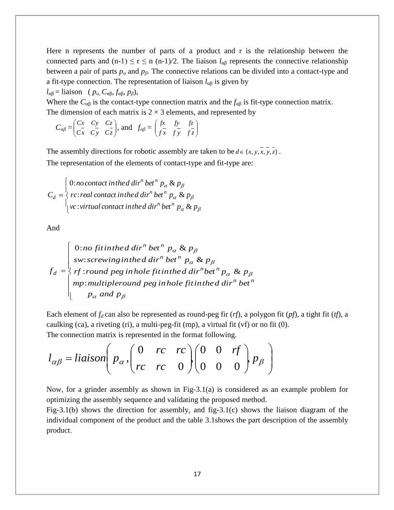
Here n represents the number of parts of a product and r is the relationship between the

connected parts and (n-1) ≤ r ≤ n (n-1)/2. The liaison lαβ represents the connective relationship

between a pair of parts pα and pβ. The connective relations can be divided into a contact-type and

a fit-type connection. The representation of liaison lαβ is given by

lαβ = liaison ( pα, Cαβ, fαβ, pβ),

Where the Cαβ is the contact-type connection matrix and the fαβ is fit-type connection matrix.

The dimension of each matrix is 2 × 3 elements, and represented by

Cαβ =

zCyCxC

CzCyCx, and fαβ =

zfyfxf

fzfyfx

The assembly directions for robotic assembly are taken to be ,,,, zyxyxd .

The representation of the elements of contact-type and fit-type are:

ppbetdirdtheincontactvirtualvc

ppbetdirdtheincontactrealrc

ppbetdirdtheincontactno

Cnn

nn

nn

d

&:

&:

&:0

And

pandp

betdirdtheinfitholeinpegroundmultiplemp

ppbetdirdtheinfitholeinpegroundrf

ppbetdirdtheinscrewingsw

ppbetdirdtheinfitno

f

nn

nn

nn

nn

d

:

&:

&:

&:0

Each element of fd can also be represented as round-peg fir (rf), a polygon fit (pf), a tight fit (tf), a

caulking (ca), a riveting (ri), a multi-peg-fit (mp), a virtual fit (vf) or no fit (0).

The connection matrix is represented in the format following.

p

rf

rcrc

rcrcpliaisonl ,

000

00,

0

0,

Now, for a grinder assembly as shown in Fig-3.1(a) is considered as an example problem for

optimizing the assembly sequence and validating the proposed method.

Fig-3.1(b) shows the direction for assembly, and fig-3.1(c) shows the liaison diagram of the

individual component of the product and the table 3.1shows the part description of the assembly

product.

18

Fig 3.1 (a) A simple example of a product (Grinder assembly), Fig 3.1(b) Directions for

assembly, Fig 3.1 (c) Liaison graph model of grinder.

Table3.1: Part description of grinder assembly

Part Symbol Part Name

a Shaft

b Blade

c Nut

d Blade

e Nut

As per the codes of the model/parts, the liaisons of the assembly components are shows as

follows:

b

oorf

ooo

rcrcrc

rcrcoaliaisonlab ,,,

c

oosw

ooo

oovc

oooaliaisonlac ,,,

d

ooo

oorf

rcrco

rcrcrcaliaisonlad ,,,

19

e

ooo

oosw

ooo

oovcaliaisonlae ,,,

c

ooo

ooo

oorc

ooobliaisonlbc ,,,

e

ooo

ooo

ooo

oorcdliaisonlde ,,,

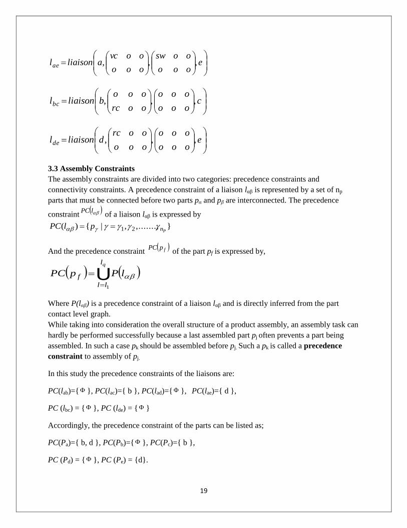
3.3 Assembly Constraints

The assembly constraints are divided into two categories: precedence constraints and

connectivity constraints. A precedence constraint of a liaison lαβ is represented by a set of np

parts that must be connected before two parts pα and pβ are interconnected. The precedence

constraint lPC

of a liaison lαβ is expressed by

,.......,,|)( 21 PnplPC

And the precedence constraint fpPC

of the part pf is expressed by,

Uql

ll

f lPpPC

1

Where P(lαβ) is a precedence constraint of a liaison lαβ and is directly inferred from the part

contact level graph.

While taking into consideration the overall structure of a product assembly, an assembly task can

hardly be performed successfully because a last assembled part pj often prevents a part being

assembled. In such a case pk should be assembled before pj. Such a pk is called a precedence

constraint to assembly of pj.

In this study the precedence constraints of the liaisons are:

PC(lab)= , PC(lac)= b , PC(lad)= , PC(lae)= d ,

PC (lbc) = , PC (lde) =

Accordingly, the precedence constraint of the parts can be listed as;

PC(Pa)= b, d , PC(Pb)= , PC(Pc)= b ,

PC (Pd) = , PC (Pe) = d.

20

3.4 Part contact level graph

The part contact level graph represents the overall structure of product assembly. In the graph,

each node is denoted by a part, while each line represents directional connection between two

parts. The assembly direction can be show d € x,y,z frame or in opposite frame. The part

contact level represents a precedence level with which a part can be assembled along a given

direction while taking into consideration the contact type connections in that particular

directions.

3.5 Feasible assembly sequence using Part Contact level graph

It is a sequence of assembling parts on a base assembly, part by part. The feasible base part is

defined as a part whose assembly precedence constraint is satisfied. At first, feasible base part

(fbp) for a product must be chosen among n parts. A feasible base part relates to the part whose

precedence constraint PC (fbp), does not exist i.e. FBP = fbp, PC (fbpi) = .

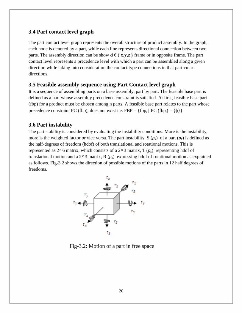
3.6 Part instability

The part stability is considered by evaluating the instability conditions. More is the instability,

more is the weighted factor or vice versa. The part instability, S (pk) of a part (pk) is defined as

the half-degrees of freedom (hdof) of both translational and rotational motions. This is

represented as 26 matrix, which consists of a 23 matrix, T (pk) representing hdof of

translational motion and a 23 matrix, R (pk) expressing hdof of rotational motion as explained

as follows. Fig-3.2 shows the direction of possible motions of the parts in 12 half degrees of

freedoms.

Fig-3.2: Motion of a part in free space

21

3.7 Summary

A systematic method of generating feasible assembly sequence has been proposed. The method

is based upon the evaluation of base assembly motion instability along with part contact level

graphs that infers the precedence constraints. To formulate a scheme for generating such a stable

sequence, instability of base assembly movement has been defined utilizing the instability of

each individual part motion. This gives the stable sequences. With the help of these, anyone can

find the most desirable sequence which yields the min no of direction changes in base assembly

movement.

22

Chapter-4

SOFT COMPUTING METHOD AND

ASSEMBLY SEQUENCE

4.1 Overview

Many types of optimization tools are available for application to the problem, like Simulated

Annealing, Evolutionary Computation, Tabu Search, Ant Colony Optimization, and Artificial

Immune System but their suitability and/or effectiveness are also under scanner. Searching the

best sequence generation involves the conventional or soft computing methods by following the

procedures of search algorithms. Intensification is an expression commonly used for the

concentration of search process on areas in search space with good quality solutions.

Diversification denotes the action of leaving already exploded areas and moving the search

process to unexplored areas. Metaheuristic is set of algorithms concepts that can be used to

define heuristic methods applicable to a wide set of different problems.

Metaheuristics are very advantageous for large search space problems. Study of various

optimization methods tells that Ant Colony Optimization (ACO) & Artificial Immune System

(AIS) method can be advantageously used to solve such problem. The concept of ACO is the

foraging behaviors of the real ant which enables them to find shortest path between a food source

and nest. It is best suitable for combinatorial optimization problem. AIS can be defines

computational system inspired by theoretical immunology, observed immune function, principle

and mechanism in order to solve problem.

4.2 Ant Colony Technique

The main concept of ACO is to imitate the cooperative manner of an ant colony to solve

combinatorial type‟s optimization problems within a reasonable amount of time. At the time of

their oath from nest to food source, ants can deposit and sniff a chemical substance known as

pheromone, which gives them with the ability to communicate with each other. An ant lays some

pheromone on the ground to mark the path it follows by trail of this substance. Ant move at

random, but when they encounter a pheromone trail, they decide whether or not to follow it. The

probability that an ant choose one path over others is determined by the amount of pheromone on

the potential path of interest. With the continuous action of the colony, the shorter path are more

frequently visited and become more attractive for subsequent ants. The main characteristics of an

ant algorithm are positive feedback, distributed computation, and the use of a constructive

greedy heuristic search.

The generic ant algorithms have four main steps as follows:

1. Initialization: Set initial population of the colony and the pheromone trail. Place starting

nodes for all ants randomly.

23

2. Solution construction: Taking into account the problem-dependent heuristic info & the

trail intensity of the path, each ant choose the next that has been visited to move by

probability. Repeat the step till a completed solution is constructed.

3. Trail update: Evaluate the solution and deposit pheromone on the solution paths

according to the quality of solution to know about solution whether it is better or not.

4. Pheromone evaporation: The pheromone trail of all paths is decreased by some constant

factor at the end of an iteration of building completed solutions.

ACO algorithms have been applied successfully in a variety of optimization problem like

Travelling salesman problem, just-in-time sequencing, and job-shop scheduling.

4.3 Artificial Immune Concept:

Like a Genetic Algorithm (GA), Artificial Immune System (AIS) is also population based and

the optimal solution is obtained by the evolution of the population. In AIS, the problems to be

solved are regarded as antigens. In general, 3 types of measurements are used to evaluate the

antibodies, namely, fitness for the quality, affinity for similarity between antibodies, &

concentration for population variety. AIS is computational intelligence paradigm inspired by the

biological immune system, which has found application in pattern recognition, scheduling,

control, machine-learning, and information system security. To implement the optimization ideas

addressed previously, immune operations including immune selection, clonal selection and

inoculation are introduced. AIS are realized by the following steps: (1) recognition of antigens;

(2) generation of initial antibodies; (3) evaluation of antibodies; (4) proliferation and suppression

of antibodies; (5) generation of new antibodies; (6) improvement of antibodies. Steps 3-6 will be

iterated until convergence criteria are satisfied.

4.4 Objective function of assembly sequence generation (ASG)

Energy function, Eseq , is associated with assembly sequence, and it is represented

as:

Eseq = EJ + EP + EC

where,

Eseq = Energy function associated with ASG

EJ = Energy related to Assembly cost

EP = Energy related to Precedence Constraints

EC = Energy related to Connectivity Constraints

where, CJ is an energy constant related to assembly sequence cost J .

The value of J can be decided as;

24

otherwiseCC

unstableisitorsconstraassembly

violatessequenceassemblyanif

J

nttass :

,int

:1

The energy associated with precedence constraints is

n

i

iPP CE1

, where, CP is a positive

constant and µi is the precedence index which is assigned to 0, if it satisfies the precedence

constraints, otherwise 1.

The energy associated with connectivity is

n

i

iCC CE1

in a similar manner connectivity index

λi is inferred on the basis of liaison relationships.

The objective of the present work is to generate feasible, stable and optimal robotic assembly

sequence with minimum assembly cost, which is linked with affinity values of artificial immune

algorithm. The objective function for the assembly is Minimize

n

i

iCiPJseq CCJCE1

)(

4.5 Degree of motion instability and the number of assembly direction changes

The possible assembly direction sets DSkcdabe s (k=c, b, a, d, e) for each part of a sequence are

expressed by

,.....2,1|:

,.....2,1|:

,.....2,1|:

,.....2,1|:

,.....2,1|:

jDdDSp

jDdDSp

jDdDSp

jDdDSp

jDdDSp

e

j

e

cbadee

d

j

d

cbaded

a

j

a

cbadea

b

j

b

cbadeb

c

j

c

cbadec

The ordered lists ),.....,2,1( miDLcbade

i of possible assembly directions corresponding to the

assembly sequence can be expressed by:

25

e

m

d

m

a

m

b

m

c

m

cbade

m

edabccbade

edabccbade

dddddDL

dddddDL

dddddDL

,,,,

,,,,

,,,,

222222

111111

The hierarchical tree of the sequence assembly directions may be represented in the format given

in the Fig-4.2 (a)

Based upon the above equation, the normalized degree of motion instability and the normalized

number of assembly direction changes are calculated. The formula for normalized motion

instability Cas is:

m

i

i

j

ijas BASim

C1 1

)12

11

where DSj (j=1,2,3,4,5) is the in-subassembly formed at the jth

assembly step, and SBAj means

the degree of motion instability of the jth

subassembly. A zero degree of motion instability means

the parts belonging to the subassembly are completely fixed to each other, whereas twelve

degrees means the parts are free to move in any direction. Similarly, the normalized number of

assembly direction changes Cnt can be expressed as:

m

i

i

j

ijnt NTim

C1 1

)(11

where (NTj) is assigned to 1 if direction change of BAj occurs for a cbade

iDL, otherwise it is 0. If

the sequence is unstable for all (DSj)is (j=1,2,3,4,5) are assigned to 1.So the number for all Cass,

and Cnts lie between 0 to 1. The zero means, the sequence completely satisfies the constraints,

and one means, unstable relationship. For a study, a possible sequence seq = c – b – a – d – e

is considered. In this study each set of possible assembly directions are represented in the format

DSkcdabe s (k=c,b a,d, e) and these are:

,,,,,,,,,, zzxDSzzxDSzzxDSxDSDS e

cbade

d

cbade

a

cbade

b

cbade

c

cbade

Fig-4.1: Parts of grinder

c

b

a

d

e

26

The order list of possible assembly directions corresponding to the assembly sequence

“c – b – a – d – e” can be obtained.

Fig-4.2 (a)

zzzxDLzxxxDLxxxxDL cbade

m

cdadecbade ,,,,,,,,,,, 21

Fig-4.3 (b)

Fig-4.2(a) Hierarchical tree structure of possible assembly direction, Fig-4.2 (b) Ordered list of

possible assembly direction.

The ordered lists ),,.....,2,1( miDLcbade

i given by the equation

e

m

d

m

a

m

b

m

c

m

cbade

m

edabccbade

edabccbade

dddddDL

dddddDL

dddddDL

,,,,

,,,,

,,,,

222222

111111

The energy matrix is having the dimension of 5n 5n matrix. Each cell represent as the energy

between two elements. In this study, each energy cell has been calculated and applied in ACO

method.

4.6 Applying ACO TO ASG

According to Marco Dorigo the basic concept of an ant colony algorithm is to solve

combinatorial problems within a reasonable amount of time. In this study, disassembly sequence

is represented as disassembly operations (DO). The sequence considered the no of parts

presented and the direction in which it is to be disassembled i.e. DO = (n, d), where „n‟ is the

27

number of components and„d‟ is the direction of disassembly. In this paper, each component is

having five possible DOs, i.e. (n, +x), (n, +y), (n, +z), (n, -x) and (n, -y). If the assembly consists

of „n‟ number of parts, then the disassembly operation is having „5n‟ number of nodes.

The disassembly operation is assigned to „1‟ if there is interference in that direction, otherwise

„0‟. That means if DO=1, it cannot be disassembled from the product. In the modified ACO

algorithms, a pheromone „ ij ‟ is used as the share memory of all ants and simultaneously it

considers the energy matrix which is to be minimized. The pheromone „ ij ‟ is updated during the

processing. Like the shortage path in TSP, this algorithm also gives the minimum energy path

which is to be follow during disassembly. In this study the pheromone is expressed as 5n X 5n

matrix as because one of the Z directions is restricted for robotic assembly.

Interference matrix in (+)ve X, Y, Z directions:-

nnznnynnxznynxnznynxn

nznynxzyxzyx

zynxzyxzyx

n

n

IIIIIIIII

IIIIIIIII

IIIIIIIII

e

e

e

DM

eee

222111

222222222212121

11111121212111111

2

1

21

where Iijd is equal to 1 if component ei interferes with the component ej during the move along

direction +d-axis; otherwise Iijd is equal to 0. The initial disassembly matrix is calculated as:

0000000000000000000010110

0000100000010000100011110

0000100001000000000110111

0000100001010000000010111

1011110111101101111000000

e

d

c

b

a

DM

yxzyxyxzyxyxzyxyxzyxyxzyx

edcba

n

j

ijddi IDO

1

)(,

And

n

j

jiddi IDO

1

)(,

11110

11111

10111

11111

11111

,,,,,

,,,,,

,,,,,

,,,,,

,,,,,

yexezeyexe

ydxdzdydxd

ycxczcycxc

ybxbzbybxb

yaxazayaxa

DODODODODO

DODODODODO

DODODODODO

DODODODODO

DODODODODO

28

Where U is the Boolean operator OR. The result will be equal to 0 if all the elements involving

in the operation are 0. This means the element can be disassembled in that direction. If the DO is

equal to 1, the element cannot be disassembled. In this study, the initial feasible disassembly

operations are (c, -x) and (e, +x).

4.7 Solution Method

Robotic assembly is a case of combinatorial optimization problem. The problem is similar to

Traveling salesman problem i.e. to give the shortest path with minimum cost. Combinatorial

optimization problem is a triple (S,f,Ω), where S is the set of candidate solutions, f is the

objective function which assigns an objective function value f(s) to each candidate solution sS,

and Ω is a set of constraints. The solutions belonging to the set of solutions S that satisfies the

constraints Ω are called feasible solutions. The stable solutions ~

belong to the feasible

solutions. One of the major advantages is that, the optimal solution satisfies all the assembly

constraints, objective function and also it is a part of stable solutions~

.

In ant system, m ants simultaneously build a solution of the ASG. Initially ants are put in first

feasible DO. At each construction step, ant k applies a probabilistic state transition rule, called

random proportional rule, to decide which node visit next.

otherwise

iCjifjiji

jiji

Pd

iCu

jid

d

,0

)(,),(),(

),(),(

)(

),(

The heuristic value selected in this study is seqE

ji1

),( .

After all the ants have constructed their tours, the pheromone trails are updated. The pheromone

evaporation is giving by ),()1(),( jiji , where 0 1 is the pheromone evaporation rate.

After evaporation, all ants deposit pheromone on the arcs they have crossed in their tour:

m

k

k jijiji

1

),(),()1(),(

Where m is the number of ants that find the iteration-best sequences and )),( jik is the amount

of pheromone ant k deposits on the arcs it has visited. It is given an equation:

29

otherwise

kantofsequencejiifjiEji k

seqk

,0

),(,),(

1

),(

Where, ),( jiEkseq is the tour energy the k

th ant belonging to that tour? During the construction of

sequences, local pheromone updating encourages exploration of alternative solutions, while

global pheromone updating encourages exploitation of the most promising solutions.

4.8 ACO Algorithm

1. Generate the initial feasible Dos and compute their quantity

2. Set the cycle counter NC = 1

3. While NC < NCmax

a. Place ants on the initial feasible nodes of the DCG

b. While each ant has not completed its tour

i. Put current DO into sequence of the ant

ii. Generate candidate list of the ant and calculate the energy

iii. Calculate of each candidate

iv. Choose next DO based on energy matrix

v. Move the ant to DO

vi. Add the component number of DO to the tabu list of the ant

vii. Locally update PM

c. Evaluate all solutions taking into account their reorientations

d. Globally update PM using iteration-best solutions

e. Update the best sequence of each ant if its iteration sequence is the best one found

so far

f. Empty the sequence, candidate list, and tabu list of each ant

g. Set

4. Output the reversed best sequence of each ant

The reverse of the output is the optimal assembly sequence generation with inverse

directions. The solution may be optimal or near optimal.

30

Start

Disassembly Completed Graph

Disassembly Matrix

Disassembly Operation

Initialize Cij and 0 ij

Place m ants at n nodes, Set s = 1, k = 1 to m,

Place the starting node of kth ant in Tabuk(s)

Generate the sequence

Is the Genn optimal ?

Update the

pheromone

intensity

Stop

N

Y

Fig 4.4- Flow diagram of the ACO procedure

31

4.9 Applying AIS to ASG

The artificial immune system was built on the two principles.

a) Clonal selection principle

b) Affinity maturation principle

Each assembly (antibody) has an energy value that refers to the affinity value of that antibody.

Affinity value of each antibody is calculated as

Affinity SeqE

p 1

Where, ESeq is the energy value of an individual assembly. For stable sequence the energy factor

is low and for unstable, it is high. The sequence constraint consists of precedence, connectivity

relationships. Lower the energy factor higher is the affinity value. The cloning of antibodies is

done directly proportional to the affinity function. More clones are generated on higher affinity

values or lower energy values.

The affinity maturation principle is defined by two methods;

Mutation and

Receptor editing.

In this study two phase mutation has been taken;

inverse mutation and

Pairwise interchange mutation.

In the first one, randomly two positions were selected and then inversed. After inversing if the

mutated sequence affinity is greater than the original one, then the mutated one is stored.

Otherwise, it will go to the pairwise mutation. Here randomly two positions were interchanged.

If the affinity value is more than the original one, then it stores the new one. Otherwise, it stores

the original one.

In receptor editing, worst percentage of antibodies were eliminated and randomly created

antibodies were replaced with them. This mechanism corresponds to new search regions in the

total search space.

32

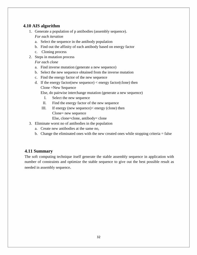
4.10 AIS algorithm

1. Generate a population of p antibodies (assembly sequence).

For each iteration

a. Select the sequence in the antibody population

b. Find out the affinity of each antibody based on energy factor

c. Cloning process

2. Steps in mutation process

For each clone

a. Find inverse mutation (generate a new sequence)

b. Select the new sequence obtained from the inverse mutation

c. Find the energy factor of the new sequence

d. If the energy factor(new sequence) < energy factor(clone) then

Clone =New Sequence

Else, do pairwise interchange mutation (generate a new sequence)

I. Select the new sequence

II. Find the energy factor of the new sequence

III. If energy (new sequence)< energy (clone) then

Clone= new sequence

Else, clone=clone, antibody= clone

3. Eliminate worst no of antibodies in the population

a. Create new antibodies at the same no,

b. Change the eliminated ones with the new created ones while stopping criteria = false

4.11 Summary

The soft computing technique itself generate the stable assembly sequence in application with

number of constraints and optimize the stable sequence to give out the best possible result as

needed in assembly sequence.

33

Chapter-5 RESULT AND DISCUSSIONS

5.1 Overview

The results obtained by using various methods for the products under consideration are

presented in the following sections. Three different kinds of approaches conventional technique

using PCLG and part instability methods along with directional precedence constraints those are

suitable and convenient for assembly sequence generation. 2nd

uses anyone of the metaheuristic

optimization tool, viz. ACO, to solve the assembly sequence generation. 3rd

uses AIS which is

computational system inspired by the theoretical immunology.

5.2 Convectional assembly sequence generation

The grinder assembly is considered example to study for inference of the feasible assembly

sequence by using the procedure of PCLG and part instability. After applying the PCLG and

part instability criteria, the following result are found out. After PCLG no of sequence found is

13, and after putting part instability criteria it reduced to 3.

We take the example of grinder assembly to strengthen the methodology. The simulation results

of selecting the parameter are taken a value between the domains of 5 to 75.

5.3 Simulation of Cj, Cp Cc

Let the product is composed to n parts and having 5n different nodes as disassembly considered

in 5 directions except the restricted motion of robot in –z direction. That means, for each part

there are 5 different assembly directions.

According that concept, the objective matrix now becomes a size of 5n x 5n nodes. Each node is

having a weighted value in connection with other nodes. If the preceding of assembly is

approaching towards instability, the value of weighted factor is rising on and vice versa. This

means that the lowest selected through iteration means the more is the stable assembly. The

assembly constraints Cj, Cp and Cc mentioned in equation are assigned random values from 5 to

75 with the increment of +5. So,

The simulation results are listed in table 5.1

Seq No.

1 a b c d e

2 b a c d e

3 d a e b c

Sequence Order

34

Energy Constants

Cost Constants

CJ CP CC t t

55 45 55 0.5 0.5

The simulation condition for ant parameter on table 5.2

Influencing

parameter of

pheromone

trail

Pheromone

Evaporation

rate

Base

part

Assembly

directions

Disassembly

directions

1 2 0.25 a zy

xyx

,

,,,

yx

zyx

,

,,,

5.4 Sample calculation

Select the partial sequence, suppose (d,( x )) – (a,( x )).

Step 1: Find-out the precedence constraints of each part. Here it is

PC(a)=b, d, PC(b)= , PC(c)= b, PC(d)= , PC(e)= d

Step 2: Precedence index are µ1 = 0, µ2 = 1

Step 3:

2

1

21 )(

i

PP CE , EP = 45 X 1= 45

Step 4:

a

oorf

ooo

rcrcrc

rcrcodlda ,,,

Step 5: λ1 is for the Cd matrix and λ2 is for the fit-type connection, here λ1 = 0, λ2 = 0

Step 6:

n

i

CC CE

1

21 )( , EC = 55 X 0= 0

Step 7: adaDS , xDSa

da , 1 aBA , 321 1 BAS

Step 8: Order list :-

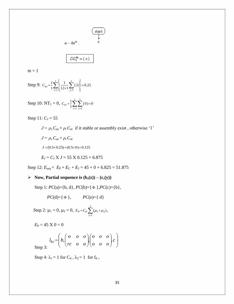
35

m = 1

Step 9: 25.0)3(112

1

1

11

1

1

1

i j

asC

Step 10: NT1 = 0,

1

1

1

1

0)0(1

1

i j

ntC

Step 11: CJ = 55

J = ρs Cas + ρt Cnt if it stable or assembly exist , otherwise „1‟

J = ρs Cas + ρt Cnt

125.0)05.0()25.05.0( J

EJ = CJ Х J = 55 Х 0.125 = 6.875

Step 12: Eseq = EP + EC + EJ = 45 + 0 + 6.825 = 51.875

Now, Partial sequence is (b,(z)) – (c,(y))

Step 1: PC(a)=b, d, PC(b)= ,PC(c)=b,

PC(d)= , PC(e)= d

Step 2: µ1 = 0, µ2 = 0,

2

1

21 )(

i

PP CE ,

EP = 45 X 0 = 0

Step 3:

c

ooo

ooo

oorc

oooblbc ,,,

Step 4: λ1 = 1 for Cd , λ2 = 1 for fd ,

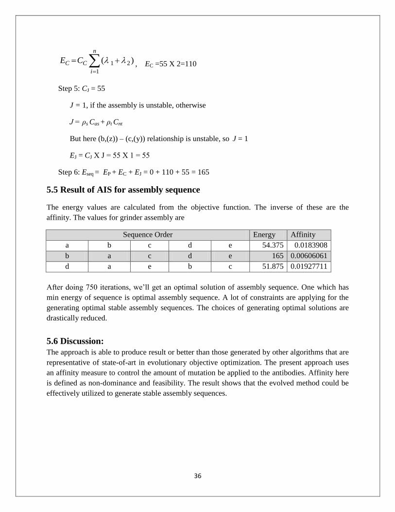
36

n

i

CC CE

1

21 )( , EC =55 X 2=110

Step 5: CJ = 55

J = 1, if the assembly is unstable, otherwise

J = ρs Cas + ρt Cnt

But here (b,(z)) – (c,(y)) relationship is unstable, so J = 1

EJ = CJ Х J = 55 Х 1 = 55

Step 6: Eseq = EP + EC + EJ = 0 + 110 + 55 = 165

5.5 Result of AIS for assembly sequence

The energy values are calculated from the objective function. The inverse of these are the

affinity. The values for grinder assembly are

Sequence Order Energy Affinity

a b c d e 54.375 0.0183908

b a c d e 165 0.00606061

d a e b c 51.875 0.01927711

After doing 750 iterations, we‟ll get an optimal solution of assembly sequence. One which has

min energy of sequence is optimal assembly sequence. A lot of constraints are applying for the

generating optimal stable assembly sequences. The choices of generating optimal solutions are

drastically reduced.

5.6 Discussion:

The approach is able to produce result or better than those generated by other algorithms that are

representative of state-of-art in evolutionary objective optimization. The present approach uses

an affinity measure to control the amount of mutation be applied to the antibodies. Affinity here

is defined as non-dominance and feasibility. The result shows that the evolved method could be

effectively utilized to generate stable assembly sequences.

37

Chapter-6

REFERENCE

1. A. Redford and J. Chal, [Book] Design for Assembly, Principle and practice, McGraw Hill

international (UK) Ltd. Important measures for Assemblability,pp.155-156.

2. G.Boothroyd, P. Dewhurst Inc., Design for Assembly Tool kit, Release 5.2, Wakefield,

Rhode Island, USA, 1991.

3. Tiam-Hock Eng, Zhi-Kui ling et al., Feature based assembly modeling and sequence

generation. Computer and Industrial Engg., 1999, Vol.36, pp.17-33.

4. J.W. Priest and J.M. Sanchez: [book] Product Development and Design for Manufacturing: A

Collaborative Approach to Producibility and Reliability (2nd edn).

5. Mikell P. Groover, [Book] Automation, Production systems and computer integrated

manufacturing, 2nd ed Prentice-Hall, USA.

6. C.K.Shin, D.S.Hong et al, Disassemblability analysis for generating robotic

assembly sequences, Proceedings of IEEE International Conference on Robotics and

Automation, 1995, pp.1284-1289.

7. Jong Hun Park and Myung Jin Chung, Automatic Generation of Assembly Sequences for

Multi-Robot Work cell. Robotics and Computer-integrated manufacturing, 1993, Vol.10,

No.3, pp.355-363.

8. C.K.Shin,H.S.Cho et al.,On the generation of robotic assembly sequences based on

separability and assembly motion stability.IEEE,1994,Vol.12,pp.7-15.

9. D.S.Hong and H.S. Cho, Optimization of Robotic Assembly Sequences using neural

Network, Proceeding of the IEEE international Conference on Intelligent Robotics and

System,1993, pp.26-30.

10. A Bourjault, "Contribution a une Approche Methodologique de L'Assemblage Automatise:

Elaboration Automatique des Sequences Operatoires, thesis dEtat (University de Besancon

Franche-Comte, 1984.

11. J.F. Wang · J.H. Liu · Y.F. Zhong to contribution on “A novel ant colony algorithm for

assembly sequence planning”

12. G.Boothroyd, P.Dewhurst, Product Design for Assembly, Boothroyd Dewhurst Inc., 2 Holley

Road, Wakefield, RI, USA. February 1987.

13. G. Boothroyd and L. Alting, "Design for assembly and disassembly", Annals CIRP,

41(2), pp. 625-636, 1992.

14. H. J. Warnecke and R. Bassler, "Design for assembly - part of the design process",

Annals CIRP, 37(1), 1988.

38

15. A.J.Scarr and P.A.Mckeown, Product Design for Automated Manufacture and Assembly.

Annals of the CIRP, 1986, Vol. 35, No. 1.

16. David W.He and Andrew Kusiak, Design of Assembly System for Modular Products. IEEE

Transactions of Robotics and Automation, 1997, Vol. 13.No.5, pp.646-652.

17. H.J Warnecke and F.Babler, Design for Assembly-Part of the Design Process. Annals of the

CIRP, 1998, Vol. 37, No.1, pp.1-4.

18. Mechanical assembly sequences,” IEEE Journal of Robotic Automation, vol. 3(6), pp. 640-

58, 1987.

19. L. S. H. De Mello, and A. C. Sanderson, “AND/OR representation of assembly plans,” IEEE

Transactions on Robotics and Automation, vol. 6(2), pp. 188-99, 1990.

20. D. Y. Cho, and H.S. Cho, “Inference on robotic assembly precedence constraints using part

contact level graph,” Robotica, vol. 11, pp. 173-183, 1993.

21. D. Y. Cho, C. K. Shin, and H. S. Cho, “Automatic inference on stable robotic assembly

sequences based upon the evaluation of base assembly motion instability,” Robotica, vol. 11,

pp. 351-62, 1993.

22. D. S. Hong, and H. S. Cho, “Optimization of robotic assembly sequences using neural-

network,” IEEE International Conference on Intelligent Robots and System, pp. 232-239,

1993.

23. D. S. Hong, and H.S. Cho, “A neural-network-based computational scheme for generating

optimized robotic assembly sequences,” Elsevier, Journal of Engineering Applications of

Artificial Intelligence, vol. 8(2), pp. 129-45, 1995.

24. S. Sharma, B.B Biswal, P.dash, B.B. choudhary on “Optimized Robotic Assembly Sequence

using ACO”.

25. T.L.De Fazio and D. E.Whitney, Simplified Generation of All Mechanical Assembly

Sequences. IEEE Journal of Robotics and Automation, 1987, Vol.3, No.6, pp.640-658;

Correction.Ibid.4:pp.705-708.

26. H.A.ElMaraghy and L. Laperriere, Modeling and sequence generation for robotized

mechanical assembly, Robotics and Autonomous Systems, 1992, Vol. 9, No. 3, pp.137-147.

27. D.Y.Cho and H.S.Cho, “Inference on robotic assembly precedence constraints using a part

level graph,”Robotica, 1993, Vol.11, pp.173-183.

28. D. Y. Cho, C. K. Shin, and H. S. Cho, “Automatic inference on stable robotic assembly

sequences based upon the evaluation of base assembly motion instability,” Robotica, 1993,

Vol. 11, pp. 351-362.

29. M. Dorigo, “Ant colony system: A cooperative learning approach to the travelling salesman

problem,” IEEE Transactions on Evolutionary Computation, 1997, Vol. 1(1), pp. 53-66.

30. Yung A. Deshmukh and J.P. Hsu-Pin Wang, Automated generation of assembly sequence

based on geometric and functional reasoning. Journal of Intelligent Manufacturing, 1993,

Vol.4, No. 4, pp. 269-84.

31. D.E.Koditschek, An approach to autonomous robot assembly.Robotica, 1994, Vol.12, No.2,

pp.137-55.

39

32. S.S.F. Smith and G.C.Smithm, Automatic stable assembly sequence generation and

evaluation. Journal of Manufacturing Systems, 2001, Vol. 20, No. 4, pp. 225-235.

33. R. B.Gottipolu and Kalyan Ghosh, A Simplified and efficient representation for evaluation

and selection of assembly sequences. Computers in Industry, 2003, Vol.50, pp. 251-264.

34. Xiaobu Yuan and S.X. Yang, Interactive assembly planning with automatic path generation.

International Conference on Intelligent Robots and Systems, 2004, Vol.4, pp.3965-3970.

35. S. Sumida, T. Suzuki et al., A Planning system for an automatic assembly robot.

Int.Symposium on industrial Robots, 1988, pp.169-178.

36. J.D.Wolter, On the automatic generation of assembly plan. In Proceedings of IEEE

International Conference on Robotics and Automation, 1989, pp.62-68.

37. D. S. Hong and H. S. Cho, "A neural-network-based computational scheme for

generating optimized robotic assembly sequences", Engineering Applications of

Artificial Intelligence, 8(2), pp. 129--145, I995.