Embed Size (px)
Citation preview

Optimization of Handover Algorithms for
Wireless Networks
SILVIA DE LUCIA
Master’s Degree Project
Stockholm, Sweden 2010

Abstract
We are witnessing a continuous development of heterogeneous wireless net-
works, such as cellular systems (e.g., the LTE, or long term evolution of the
third generation wireless system), sensor networks, and satellite networks.
The coexistence of all these networks requires the design of control mech-
anisms to allow the seamless communication from one network to another,
and even between communication standards. The handover is one such con-
trol mechanism. Specifically, the handover is the mechanism of transferring
the connection of a mobile node from an access point (which could be a base
station or a network using some communication standard) to another AP.
During the handover, a node that is being disconnected from an AP and con-
nected to another AP may experience a sudden degradation of the bandwidth
or outage of the communication. This leads to frequent and unnecessary han-
dovers that may reduce significantly the quality of service perceived by the
node. Therefore, in order for the node to achieve high quality of service, an
optimization of the handover algorithm is essential. In this thesis we study
some optimization algorithms for the handover procedure. We show that
the variables available at the node to control the handover are the hysteresis
margin, which is used to compare the quality of signals of the APs, and the
estimation window length, which is the number of samples to estimate with a
desired accuracy these signals. Then, we study two optimization problems in
which the parameters that affect the handover are optimized by considering
as a cost function a convex combination of the probability of outage and the
probability of handover. The first problem is based on a static optimization,
whereas the second problem on a dynamic optimization. We show that both
problems offer better performance with respect to existing algorithms from
the literature. We show that the dynamic optimization gives better results,
but at the cost of an increased computational complexity.
I

Contents
Abstract . . . . . . . . . . . . . . . . . . . . . . . . . . . . . . . . . I
1 Introduction to Handover 1
1.1 Handover procedure . . . . . . . . . . . . . . . . . . . . . . . . 1
1.2 Types of Handover . . . . . . . . . . . . . . . . . . . . . . . . 2
1.3 Handover initiation . . . . . . . . . . . . . . . . . . . . . . . . 2
1.4 Handover Decison . . . . . . . . . . . . . . . . . . . . . . . . . 3
1.5 Handover in Microcellular Propagation Environment . . . . . 5
1.6 Handover in Multihop Cellular Networks . . . . . . . . . . . . 6
1.7 Handover scenarios in MCNs . . . . . . . . . . . . . . . . . . . 6
1.8 Handover in IP Networks . . . . . . . . . . . . . . . . . . . . . 9
1.9 Mobility in 6LoWPAN . . . . . . . . . . . . . . . . . . . . . . 11
1.9.1 Application methods . . . . . . . . . . . . . . . . . . . 12
1.9.2 Mobile IPv6 on 6LoWPAN . . . . . . . . . . . . . . . . 13
1.9.3 NEMO . . . . . . . . . . . . . . . . . . . . . . . . . . . 13
2 Problem Formulation 15
3 Modeling 18
3.1 System Model . . . . . . . . . . . . . . . . . . . . . . . . . . . 18
3.2 Least Square Algorithm: Performance Measures . . . . . . . . 19
3.2.1 Handover decision an probabilities . . . . . . . . . . . . 21
3.3 The effect of the Hysteresis Margin . . . . . . . . . . . . . . . 24
3.3.1 Probability of Base Station Connection . . . . . . . . . 24
3.3.2 Probability of Handover and Probability of Outage . . 26
3.4 Approximations . . . . . . . . . . . . . . . . . . . . . . . . . . 27
3.4.1 First Bound . . . . . . . . . . . . . . . . . . . . . . . . 27
3.4.2 Second Approximation: proposed bound . . . . . . . . 28
II

4 Optimization 30
4.1 Pareto Optimization of the Estimate Window Length . . . . . 30
4.2 Static Handover and Outage Pareto Optimization . . . . . . . 31
4.3 Optimization of the Probability of Handover . . . . . . . . . . 32
4.4 Probability of Outage Optimization . . . . . . . . . . . . . . . 33
4.5 Dynamic Handover and Outage Pareto Optimization . . . . . 33
5 Simulation Results 36
5.1 Probability of Handover and Probability of Outage . . . . . . 36
5.2 Estimate Window Length Pareto Optimization Results . . . . 39
5.3 Approximations results . . . . . . . . . . . . . . . . . . . . . . 40
5.3.1 First approximation . . . . . . . . . . . . . . . . . . . 40
5.3.2 Second approximation . . . . . . . . . . . . . . . . . . 41
5.4 Performance Evaluation of Hysteresis Optimization . . . . . . 44
5.4.1 Static Optimization Results . . . . . . . . . . . . . . . 44
5.4.2 Dynamic Optimization Results . . . . . . . . . . . . . 48
5.4.3 Improving Factors . . . . . . . . . . . . . . . . . . . . 50
6 Conclusions 52
III

List of Figures
1.1 Soft and Hard handover . . . . . . . . . . . . . . . . . . . . . . 2
1.2 Signal strength and hysteresis between two adjacent BSs for po-
tential handover. . . . . . . . . . . . . . . . . . . . . . . . . . . 3
1.3 Handover scenarios in Microcellular Networks (MCN) . . . . . . . 5
1.4 Handover scenarios in MCN; BS is the base station, MS is the
mobile station, RS is the relay station and a Cell is a coverage
area of the BS . . . . . . . . . . . . . . . . . . . . . . . . . . . 6
1.5 Optimized vertical handover framework . . . . . . . . . . . . . . 11
3.1 The hysteresis of the handover decision. . . . . . . . . . . . . . . 24
4.1 Trellis diagram for the computation of outage probabilities in the
dynamic optimization. . . . . . . . . . . . . . . . . . . . . . . . 34
4.2 Trellis diagram for the computation of handover probabilities in
the dynamic optimization. . . . . . . . . . . . . . . . . . . . . . 34
4.3 Optimization scheme . . . . . . . . . . . . . . . . . . . . . . . . 34
5.1 Probability of handover versus distance d0 for LS method. The
parameter is the window length nw. . . . . . . . . . . . . . . . . 37
5.2 Probability of outage versus distance d0 for LS method. The pa-
rameter is the window length nw. . . . . . . . . . . . . . . . . . 37
5.3 Maximum values of outage probability versus estimate window
length. . . . . . . . . . . . . . . . . . . . . . . . . . . . . . . . 37
5.4 Maximum values of handover probability versus estimate window
length. . . . . . . . . . . . . . . . . . . . . . . . . . . . . . . . 37
5.5 Handover and outage probability evaluate at nw optimum for the
problem having the objective function in (4.6) . . . . . . . . . . . 39
5.6 Probability of BSs connection versus distance for the first bound
proposed in Section 3.4 . . . . . . . . . . . . . . . . . . . . . . . 40
IV

5.7 Probability of handover versus distance evaluated by using the sec-
ond approximation given by equation (3.19) in Chapter 3, with
nw = 10 . . . . . . . . . . . . . . . . . . . . . . . . . . . . . . 41
5.8 Probability of handover versus distance evaluated by using the sec-
ond approximation given by equation (3.19) in Chapter 3, with
nw = 40 . . . . . . . . . . . . . . . . . . . . . . . . . . . . . . 41
5.9 Probability of outage versus distance evaluated by using the second
approximation given by equation (3.19) in Chapter 3, with nw = 10 42
5.10 Probability of outage versus distance evaluated by using the second
approximation given by equation (3.19) in Chapter 3, with nw = 40 42
5.11 Comparison between handover probability values for different
m . . . . . . . . . . . . . . . . . . . . . . . . . . . . . . . . . . 43
5.12 Comparison between outage probability values for different m 43
5.13 Handover probability evaluated at optimum h for the static opti-
mization problem. . . . . . . . . . . . . . . . . . . . . . . . . . 44
5.14 Outage probability evaluated at optimum h for the static optimiza-
tion problem. . . . . . . . . . . . . . . . . . . . . . . . . . . . . 44
5.15 Objective function evaluated at optimum h for the static optimiza-
tion problem. . . . . . . . . . . . . . . . . . . . . . . . . . . . . 45
5.16 Handover and Outage probabilities evaluated by setting a fixed
histeresis margin h=2: no optimization . . . . . . . . . . . . . 46
5.17 Objective function evaluated by setting h=2: no optimization . . . 46
5.18 Handover and Outage probability evaluated by setting a fixed
histeresis margin h=8: no optimization . . . . . . . . . . . . . 46
5.19 Objective function evaluated by setting h=8: no optimization . . . 47
5.20 Comparison between objective functions evaluate at hopt by apply-
ing dynamic and static optimization techniques with a weigthing
cofficient equal to 0.5 . . . . . . . . . . . . . . . . . . . . . . . . 48
5.21 Comparison between objective functions evaluate at hopt by apply-
ing dynamic and static optimization techniques with a weigthing
cofficient equal to 0.8 . . . . . . . . . . . . . . . . . . . . . . . . 48
5.22 Comparison between objective functions evaluate at hopt by apply-
ing dynamic and static optimization techniques with a weigthing
cofficient equal to 0.2 . . . . . . . . . . . . . . . . . . . . . . . . 49
5.23 Improving factor between objective function evaluated by fixing
an hysteresis margin h = 2 and the objective function at hopt
computed by using the static optimization . . . . . . . . . . . . . 51
V

5.24 Improving factor between objective function evaluated by fixing
an hysteresis margin h = 2 and the objective function at hopt
computed by using the dynamic optimization . . . . . . . . . . . 51
5.25 Improving factor between objective function evaluated by fixing
an hysteresis margin h = 8 and the objective function at hopt
computed by using the dynamic optimization . . . . . . . . . . . 51
5.26 Improving factor between objective function evaluated by fixing
an hysteresis margin h = 8 and the objective function at hopt
computed by using the dynamic optimization . . . . . . . . . . . 51
5.27 Improving factor between objective function evaluated by using
static and dynamic optimization. The value of the parameter α is
0.2 . . . . . . . . . . . . . . . . . . . . . . . . . . . . . . . . . 51
VI

Chapter 1
Introduction to Handover
In a wireless network the need of managing the receivers mobility and ensur-
ing continuous service led to the develop of procedures for a good network
performance. This is achived by supporting the handover (or handoff ) al-
gorithm, which is a procedure that can be applyed to every kind of wireless
communication network and it is also possible within the same radio system
or between heterogeneous systems wich are standardized by protocols devel-
oped by different standardization bodies. In this chapter, we present the
main characteristics of the handover algorithm.
1.1 Handover procedure
The handover is the key to enable function for mobility and service conti-
nuity among a variety of wireless access technologies. It is is the process
of changing channel (frequency, time slot, spreading code, or combination
of them) associated with the current connection while a communication is
in progress. In cellular telecommunications the term handover refers to the
procedure of transferring a call or a data section while the mobile station is
moving away from a coverage area, called cell, to another cell. This process
is carried out to avoid the interruption of an in-progress call when the mobile
gets outside the range of the cell. In fact a handover initiation is the process
by which a handover is started as a consequence of the fact that the cur-
rent link is unacceptably degraded and/or another base station can provide
a better communication link.
1

CHAPTER 1. INTRODUCTION TO HANDOVER 2
BS0 BS0BS1 BS1MS MS
a. Soft handover b. Hard handover
Figure 1.1: Soft and Hard handover
1.2 Types of Handover
It is possible to distinguish between Hard Handover and Soft Handover.
In the soft handover the mobile station is simultneously connected to two
different base stations (see Fig. 1.1a). On the contrary, in the hard the
connection to the serving base station is interrupted while the new base
station takes on the connection (Fig. 1.1b). Furthermore hard handover can
be divided into intracell handover and intercell handover; the soft handover
can also be divided into multiway soft handover and softer handover. Soft
handover is highly expensive for the network, but offers potentially a higher
performance with respect to the hard handover. Nevertheless, the recent
standardizations of new technologies of Long Term Evolution (LTE) and
High Speed Packet Access (HSPA) suggest the use of hard handover only.
1.3 Handover initiation
The decision to initiate a handover at a mobile station may be based on
different measurements, e.g. the recived signal strenght from the serving base
station and neighboring base stations (BS’s), the distance from BS’s, and the
bit error rate. Handover is critical in cellular communication systems because
neighboring cells are always using a disjoint subset of frequency bands, so
negotiations must take place between the mobile station (MS), the current
BS, and the next potential BS.

CHAPTER 1. INTRODUCTION TO HANDOVER 3
Relative signal strength
This method works by selecting the BS from which the strongest signal is
received. The decision is based on the computation of the average of the
measurements of the received signal. It has been observed that this method
generates many unnecessary handovers, even when the signal of the current
BS is still at an acceptable level. Some variations have been proposed, as we
see in the following.
Relative signal strength with threshold
This method allows a MS to hand off only if the current signal is sufficiently
weak (less than threshold) and the other is the stronger of the two. The
effect of the threshold depends on its relative value as compared to the signal
strengths of the two BSs at the point at which they are equal.
Signal strength Signal strength
BS0 BS1
T1
T2
T3
A B C D
h
MS
Figure 1.2: Signal strength and hysteresis between two adjacent BSs for potential
handover.
If the threshold is higher than this value, say T1 in Fig. 1.2, this scheme
performs exactly as the relative signal strength scheme, so the handoff occurs
at position A. If the threshold is lower than this value, say T2 in Fig. 1.2, the
MS would delay handoff until the current signal level crosses the threshold at
position B. In the case of T3, the delay may be so long that the MS drifts too
far into the new cell. This reduces the quality of the communication link from

CHAPTER 1. INTRODUCTION TO HANDOVER 4
BS1 and may result in a dropped call. Moreover, this results in additional
interference to cochannel users. Thus, this scheme may create overlapping
cell coverage areas. A threshold is not used alone in actual practice because
its effectiveness depends on prior knowledge of the crossover signal strength
between the current and candidate BSs.
Relative signal strength with hysteresis
This scheme allows a user to hand off only if the new BS is sufficiently
stronger (by a hysteresis margin, h in Fig. 1.2) than the current one. In
this case, the handover would occur at point C. This technique prevents the
so-called ping-pong effect, the repeated handover between two BSs caused
by rapid fluctuations in the received signal strengths from both BSs. The
first handover, however, may be unnecessary if the serving BS is sufficiently
strong.
1.4 Handover Decison
There are numerous methods to perform handover, at least as many as the
type of network entities that maintain the state information. The decision-
making process of handover may be centralized or decentralized (i.e. the
handover decision may be made at the MS or at in the core network). From
the decision process point of view, it is possible to find at least three different
kinds of handoff decisions.
Network-Controlled Handover
In a network-controlled handover protocol, the network makes a handover
decision based on the measurements on the MSs at a number of BSs. In
general, the handover process (including data transmission, channel switch-
ing, and network switching) takes 100–200 ms. Information about the signal
quality for all users is available at a single point in the network that facili-
tates appropriate resource allocation. Network-controlled handoff was used
in first-generation analog systems such as AMPS (advanced mobile phone
system), TACS (total access communication system), and NMT (advanced
mobile phone system).

CHAPTER 1. INTRODUCTION TO HANDOVER 5
Mobile-Assisted Handover
In a mobile-assisted handover process, the MS makes measurements that are
transmitted to the network to let it able to make the decision. In analog
systems handover procedure is entirely carried on by the network, in the
circuit-switched GSM (global system mobile) is a mobile assisted procedure.
This mainly means that handover algorithm can operate more efficiently ac-
cording to the larger number of available parameters. The handover time
between handover decision and execution in a circuit-switched GSM is ap-
proximately 1 second.
Mobile-Controlled Handover
In mobile-controlled handover, each MS is completely in control of the han-
dover process. This type of handover has a short reaction time (on the order
of 0.1 second). MS measures the signal strengths from surrounding BSs and
interference levels on all channels. A handover can be initiated if the signal
strength of the serving BS is lower than that of another BS by a certain
threshold.
1.5 Handover in Microcellular Propagation
Environment
In a microcellular propagation environment there are two possible handovers:
handover in line-of-sight (LOS) and handover in non line-of-sight (NLOS).
To study the role of the hysteresis, Murase [8] analized the two cases: for
LOS handover the MS always mantains a LOS with both the serving and the
target BS. This is the case, for example, when a MS traverses along a route
from BS0 to BS2 in Fig. 1.3. NLOS handover, instead, arises when the MS
suddenly loses the LOS component with the serving BS while gaining a LOS
component with the target BS. This phenomenon is called the corner effect,
since it occurs while turning corners in urban microcellular settings as the
one shown in Fig. 1.3 where the MS traverses along a route from BS0 to BS1.
In this case, the average recived signal strength can drop by 25-30 dB over
distance as small as 10 m. Corner effects may also cause link quality imbal-
ances on the forward and reverse channels due to the following mechanism.
Quite often the co-channel interference will arrive via a NLOS propagation

CHAPTER 1. INTRODUCTION TO HANDOVER 6
BS0
BS1
BS3
BS2
250 m
Figure 1.3: Handover scenarios in Microcellular Networks (MCN)
path. Hence, as a MS rounds a corner, the recived signal strength at the
sertving BS suffers a large decrease while the NLOS co-channel interference
remains the same, i.e., the corner effect severly degrades the carrier to inter-
ference ratio (C/I). Meanwhile, the corner will cause the same attenuation
to both the desired and interfering signals that are recived at the MS. There-
fore, unless there are other sources of co-channel interference that become
predominant as the MS round the corner, the C/I on the forward channel will
remain about the same. If the handover requests from rapidly moving MSs in
microcellular network are not processed quickly, then excessive dropped calls
will occur. Fast temporal based handover algorithms can partially solve this
problem; these algorithms make use of temporal averaging windows that are
used to detect drops in signal strength. However, the effectiveness of these
algorithms depends on the velocity of the MS. Adaptive handover algorithms
can overcome these problems in propagation environments that are typical
of urban microcellular networks.
1.6 Handover in Multihop Cellular Networks
In conventional cellular systems handover occurs only when a mobile station
(MS) moves to different cell or different sectors of the same cell. The intro-
duction of next generation wireless systems, such as fourth generation (4G),

CHAPTER 1. INTRODUCTION TO HANDOVER 7
Cell 1 Cell 2
MS1
MS2MS3
MS4
MS5
BS1 BS2
RS1a
RS1b
RS1c
RS1d
RS2a
RS2b
RS2c
RS2d
Scenario1Scenario2
Scenario3
Scenario5
Scenario4
Figure 1.4: Handover scenarios in MCN; BS is the base station, MS is the mobile
station, RS is the relay station and a Cell is a coverage area of the BS
Third Generation Partnership Project Long-Term Evolution (3GPP LTE),
and IEEE 802.16m includes the development of multihop cellular networks
(MCN) to increase the cell radius or combat the shadowing effect, which is
mainly caused by large obstacles between transceivers.
As shown in Fig. 1.4 in MCN additional handover occur between the BS
and relay stations (RSs) or two different RSs. These additional MCN han-
dovers can cause serious ping pong problems and increase signalling overhead.
Although there are works where relay handover problems is explained, the
main interest of using the multihop concept is not in cellular networks but in
ad-hoc networks; unfortunately doesn’t exist a rich body of literature about
applications of handover in multi-hop networks.
1.7 Handover scenarios in MCNs
There are several possible handover scenarios in MCNs regardless of the RS
deployment structure. Handovers in MCNs can occur when an MS moves
between different BSs, between different RSs, or between a BS and an RS as
shown in Fig. 1.4
CHAPTER 1. INTRODUCTION TO HANDOVER 8
Intracell handover
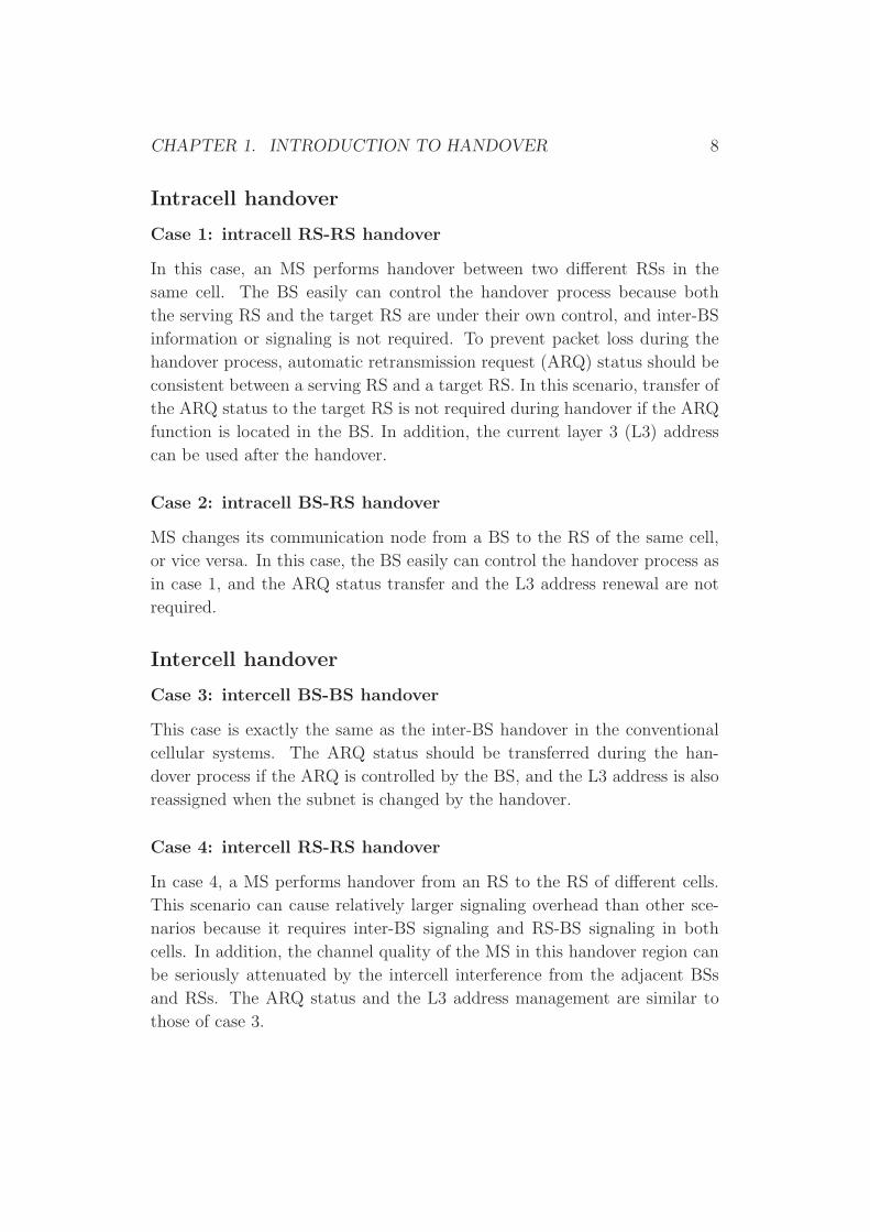
Case 1: intracell RS-RS handover
In this case, an MS performs handover between two different RSs in the
same cell. The BS easily can control the handover process because both
the serving RS and the target RS are under their own control, and inter-BS
information or signaling is not required. To prevent packet loss during the
handover process, automatic retransmission request (ARQ) status should be
consistent between a serving RS and a target RS. In this scenario, transfer of
the ARQ status to the target RS is not required during handover if the ARQ
function is located in the BS. In addition, the current layer 3 (L3) address
can be used after the handover.
Case 2: intracell BS-RS handover
MS changes its communication node from a BS to the RS of the same cell,
or vice versa. In this case, the BS easily can control the handover process as
in case 1, and the ARQ status transfer and the L3 address renewal are not
required.
Intercell handover
Case 3: intercell BS-BS handover
This case is exactly the same as the inter-BS handover in the conventional
cellular systems. The ARQ status should be transferred during the han-
dover process if the ARQ is controlled by the BS, and the L3 address is also
reassigned when the subnet is changed by the handover.
Case 4: intercell RS-RS handover
In case 4, a MS performs handover from an RS to the RS of different cells.
This scenario can cause relatively larger signaling overhead than other sce-
narios because it requires inter-BS signaling and RS-BS signaling in both
cells. In addition, the channel quality of the MS in this handover region can
be seriously attenuated by the intercell interference from the adjacent BSs
and RSs. The ARQ status and the L3 address management are similar to
those of case 3.

CHAPTER 1. INTRODUCTION TO HANDOVER 9
Case 5: intercell BS-RS handover
In this case an MS moves from a BS to the RS of different cells, or vice versa.
Inter-BS signaling is also required in this scenario, and the ARQ status and
the L3 address management are the same as scenario 3 except for additional
signaling between the RS and the BS.
Received-Signal-Strength Measurement and Handover
Decision
The received-signal-strength (RSS) measurement process can cause packet-
loss or packet-transmission delay because an MS cannot receive data packets
from the serving BS during the RSS measurement for the neighbor BSs. In
an MCN, the RSS measurement overhead increases because an MS should
measure the RSS of the neighbor RSs, as well as the neighbor BSs. There-
fore, packet-loss or packet-transmission delay caused by handover can be
increased in an MCN compared to a singlehop cellular network (SCN). The
handover decision is based on the RSS measurement result. When the serving
BS receives the measurement report from the MS or the RS, it determines
the handover execution and direction based on the RSS and the resource
availability in the target BS or RS.
Handover Procedures and Signaling
Regardless the exchange of specific messages during the handover execution
which are different according to the scenario, it is possible to say that the
handover procedure consists of several steps such as measurement, handover
decision, handover ranging, association, and resource allocation.
Handover Latency and Service-Interruption Time
There are two important performance metrics of handover schemes:
• handover latency
• service-interruption time
Handover latency is defined as the duration between the time when the
measurement procedure starts and the time when the Handover-Complete

CHAPTER 1. INTRODUCTION TO HANDOVER 10
message (which indicates the end of handover process) is transmitted to a
serving BS. To clarify, handover starts with the mesurement procedure per-
formed by the MS and after wich a serving BS determines the handover ex-
ecution and direction, whereas an HandoverComplete message comes before
the Connection release step wich completes the whole handover procedure.
This parameter can be calculated differently according to the scenario.
The service-interruption time can be defined as the duration from suspend-
ing data transmission to resuming data transmission, triggered by the RSS
measurement and handover completion, respectively. In intracell handover
scenarios, the service interruption occurs only during the measurement pro-
cedure if the puncturing or addition finger in the receiving module of an
MS is not considered. However, in intercell handover scenarios, the service
interruption can occur during the measurement and handover execution pro-
cedures.
Considerations on MCNs handover
Several design principles can affect the performance of handover schemes in
an MCN. The location and number of RSs in a cell for an MCN have the
most direct impact on the performance of handover in terms of throughput
and handover latency. With an appropriate handover scheme it is possible,
for example, improve the overall cell throughput, simplifie the handover pro-
cess, reduce handover signaling overhead and handover latency, and improve
significantly the service-interruption time. The choice of the scheme should
be a compromise between technical issues and network complexity.
1.8 Handover in IP Networks
Cellular networks are evolving to provide not only the traditional voice ser-
vice but also data services. IP appears to be the base technology of future
networks, to provide all kind of services and through different access tech-
nologies, both fixed and mobile. In Ip networks the management of terminal
mobility is achived by using the Mobile IP (MIP) protocol wich makes use
of two addresses for the mobile:
• a long term address (home address)
• a short-term local address (care of address, CoA)

CHAPTER 1. INTRODUCTION TO HANDOVER 11
The home address belongs to the MT’s home domain, while CoA belongs
to the visiting network and it is used by the mobile when it is away from
the home network. The home address is used as endpoint identifier for the
transport layer, while the CoA is used as location identifier.
Enhanced Mobile Internet Protocols
The basic MIP scheme is not efficient in certain circumstances, this due
to an handover delay introduction wich is often unaccetable for real time
applications. Wether to make faster some procedures like movement detec-
tion, new CoA configuration and location update, and to improve mobile
communications, enhancements to the Mobile IP technique, such as MIPv6,
Faster MIPv6 (FMIPv6) and Hierarchical MIPv6 (HMIPv6), are being de-
veloped. All these protocols are host-based in the sense that the MTs needs
to implement mobility-related functionality to perform handover and loca-
tion management signaling when they move between network subnets. Re-
cently the Internet Engineering Task Force IETF specified a network-based
localized mobility management protocol that allows MTs to move between
subnets within the same access network without requiring changes in their
IPv6 protocol stack. This protocol is called Proxy MIPv6. Although the
current trend in network-layer mobility management protocol design is to
enhance the level of coordination between distinct network entities, efficient
handover is required also for close interaction of functions inside the entities
themselves. This interaction is essential to reduce the delays associated with
handover operation.
IEEE 802.21 based vertical handover framework
The IEEE 802.21 is the standard that provides services facilitating handovers
between heterogeneous networks and an optimized handover framework that
leverages genric link-layer intelligence independent of the specifics of mo-
bile nodes or radio access networks. In this regard, the mobility manage-
ment protocol stack of the network elements engaged in handover signaling
is readdressed, and a logical entity is introduced between the link and up-
per layers. This entity, called MIH function (MIHF), provides tree kind of
services: event, command and information services to its users. To provide
these services a group of primitives included in a media-independent service

CHAPTER 1. INTRODUCTION TO HANDOVER 12
Upper Layers
MIH_SAP
MIHF
MIH_LINK_SAP
802.11 802.16 3GPP DVB
Mobile terminal
Figure 1.5: Optimized vertical handover framework
access point (SAP) MIH-SAP are used; on the other hand, to communicate
with link layers the MIHF uses primitives that are defined in the media-
dependant MIH-LINK-SAP and mapped to technology-specific primitives.
The architecture is shown in Fig. 1.5. MIHF facilitates handover initiation
(network discovery, network selection, handover negotiation) and handover
preparation (link 2 and link 3 connectivity, resource reservation).
1.9 Mobility in 6LoWPAN
Today’s increasing use of embedded devices, also called smart objects, that
are universally becoming IP enabled and an integral part of the internet
(Internet-connected), led to the definition of the so-called Internet of Things.
6LoWPAN is a set of standards defined by the Internet Engineering Task
Force (IETF) enabling the efficient use of IPv6 over low-pass, low-rate wire-
less networks on simple embedded devices through an adaptation layer and
the optimization of related protocols [3]. There is a wide range of applications
where 6LoWPAN technology may be used, for example home and building
automation, real-time environmental monitoring and forecasting, industrial

CHAPTER 1. INTRODUCTION TO HANDOVER 13
automation, personal health and fitness. In these scenarios is useful to con-
sider the mobility because in some cases, such as with body area networks,
the network itself may even be mobile. Mobility is often associated with
topology change so there are several reasons why it happens:
• Physical Movement: the devices change their point of attchment.
• Radio Channel: change in radio propagation may be caused by en-
vironmental change and this often require different topology.
• Network performance: in a wireless network poor signal strength,
node congestion and collisions cause packet loss and delay that reduce
network performance and induce a node to change its attachment point.
• Sleep schedules: in a wireless embedded network, to save battery
power, node use sleep schedules. If a node is attached to a sleeping
router it will move to a better point of attachment.
• Node failure: the failure of a router causes a topology change for
nodes using it as their default router.
In IP networks, mobility is the change of the attachment point of the node.
Mobility may be distinguish in two kinds [3]:
• Roaming: node moves to another network typically without packets
stream.
• Handover: node changes its attachment point during the packets trans-
mission to and from the network. In order for the mobile node to com-
municate again, this process may include operations at specific link
layers as well as at the IP layer.
Further, it is possible to distinguish between micro-mobility and macro-
mobility; in 6LoWPAN micro-mobility refers to the mobility of a node within
a LoWPAN where the IPv6 prefix does not change thus such a mobility re-
quires only the handover, macro-mobility, instead, refers to mobility between
LoWPANs in which the IPv6 changes, and it requires both routing and han-
dover. Another class of mobility is the network mobility that concerns the
changing of the attachment point of an entire network.

CHAPTER 1. INTRODUCTION TO HANDOVER 14
Solutions for mobility
As well known each node manage the mobility involving different layers of
the protocol stack. Depending on the type of mobility that occurred and
the handover and roaming prcedures that are in use there are more or less
layers involved. If the node movement is contained within the same LoWPAN
network the link layer may be able to deal with the mobility without any
noticeable change to the network layer. Common link layers that deal with
the mobility include cellular systems such as GPRS or UMTS which perform
handovers maintaining the same IP address; low-power wireless link-layer
technologies such as IEEE 802.15.4 tend to leave mobility to be dealt with
by the network layer. Networks such as IEEE 802.15.4 work in a manner
that all topology changes are node-controlled rather than network-controlled
(such as in cellular systems). If the node moves between different LoWPANs
it needs to change the IPv6 address; if a node acts as a client, a simple way
to deal with such an address change is for the applications to restart when
detecting a change in IP address. A real challenge is to manage the macro-
mobility if a node acts as a server: a way to deal with this in 6LoWPAN
applications is making use at application layer of session initiation protocol
(SIP), uniform resource identifiers (URIs) or a domain name server (DNS).
1.9.1 Application methods
If the LoWPAN network layer does not use mechanisms for the mobility, the
handover causes effects at the application layer. Dealing with mobility at
this layer may even provide better optimization for some applications. For
an application server communicating with mobile 6LoWPAN Nodes with
changing IP address to function, it needs to use some sort of unique and
stable identifier for each node. Examples include the EUI-64 of the node’s
interface, a URI, a universally unique identifier (UUID) or for example a
domanin name.
1.9.2 Mobile IPv6 on 6LoWPAN
As explained in the previous section, the mobility of nodes on the Internet
is managed by using the MIP protocol. As 6LoWPAN is an adaption for
IPv6, it would make sense to apply MIPv6 for dealing with the mobility in
6LoWPAN Nodes while maintaining a costant IPv6 address. The limit to

CHAPTER 1. INTRODUCTION TO HANDOVER 15
the use of the MIPv6 for 6LoWPAN is due to the node complexity, power
consumption and limited bandwidth of wireless links that make it difficult to
apply on this field. In order to be applied to 6LoWPAN Node mobility, the
MIPv6 would be to be implemented on LoWPAN Nodes but this problem is
still under investigation. In this regards there are some proposals:
• To full MIPv6 messages are compressed and decompressed by edge
routers; this technique would need a standardization;
• The edge router or some other entity on the visited network would
proxy MIPv6 functions on behalf of the LoWPAN Nodes (proxy method).
1.9.3 NEMO
IP, IPv4, IPv6 were not designed to take into account mobility of users and
terminals. But some IP-layer protocols, such as MIPv6, that the IETF has
defined to enable terminal mobility in IP networks exists. Nevertheless, these
protocols do not support the movement of a complete network that moves
as a whole changing its point of attachment to the fixed infrastructure, that
is, network mobility. A solution to this problem is provided by a working
group called NEMO or network mobility [4]. The NEMO protocol works
by introducing a new logical entity called the mobile router that is able to
deal with MIPv6 and is responsible for handling its function for the entire
mobile network. The network consists of a number of nodes called mobile
network nodes (MNNs) and each node does not need to run Mobile IP be-
cause the router are attached to runs Mobile IP. When the entire LoWPAN,
including edge router and MNNs associated to it, move togheter to a new
point of attachment, applying NEMO means having benefits because inside
the LoWPAN no change can be noticed due to network mobility. The edge
router, in fact, acts as a NEMO mobile router: using MIPv6 binds its new
care-of address in the visited network, and in addition the home LoWPAN
prefix. This means that the LoWPAN continues to use the same prefix as in
the home network.

Chapter 2
Problem Formulation
The handover is the procedure that allows user’s mobility in the context of
heterogeneous -or not- wireless networks by ensuring continuity of service; in
this scenario outage events, that are defined as periods in which the recived
signal level is not sufficiently high to prevent the session interruption, must
be considered to achive a good quality of service. In a wireless network, it is
necessary to minimize outage events, because they reduce the quality of the
communicaiton, and optimize the number of handovers, because they are very
expensive to manage. This thesis focus on the probability of handover and the
probability of outage optimization with respect to important parameters in
the handover initiation: the estimate window length and hysteresis margin.
In effect, a variety of parameters such as bit error rate (BER), carrier-to-
interference ratio (C/I), distance, traffic load, signal strength, and various
combination of them have been suggested in literature for evaluating the link
quality and deciding when a handover should be performed, as we explained
in the previous chapter. Signal strength measurement is one of the most
common criterion, and it is considered in this work. To improve performance,
optimization with respect to some key parameters of the handover algorithm
are studied in this thesis. We consider the LS algorithm proposed in [1],
and we will first evaluate the probabilities of handover (PH) and outage (PO)
for a mobile station (MS) moving between a certain number of base stations
(BSs); then we will study an optimization of the probabilities with respect to
the value of the estimate window length nw, which is the number of samples
to use to make an estimate of the power of the received signals from the base
stations. This parameter plays a foundamental role in terms of performance
since it affects PH and PO. As will be shown in Chapter 5, an increase of
16

CHAPTER 2. PROBLEM FORMULATION 17
nw causes a decrease of PH and an increase of PO, thus a suitable balance
between higher values of PO and lower values of PH has to be found. The
optimal nw is obtained by solving a static optimization problem, which makes
use of the following objective function:
Fobj(n, nw) = α · PH(n, nw) + (1 − α) · PO(n, nw),
where PH(n) is the handover probability at time n, PO(n) is the outage
probability at time n, α is a weighting coefficient. We study how to chose
nw so that the objective function is minimized at each time n. Moreover, we
study the case when an hysteresis margin h is introduced (see the previous
chapter). We then study how to optimize the objective function for such an
hysteresis margin. We will consider two optimizations: a static one and a
dynamic one. Static optimization means that the minimization looks only at
present time and does not take into account what happens in future moments,
that is what is done in the dynamic one. By using the hysteresis margin, the
cost function is defined as follows:
J(n, h(n)) = α · PH(h(n), n) + (1 − α)PO(h(n), n). (2.1)
The static optimization problem is expressed by:
minh(n)
J(n, h(n)),
Notice that the left hand side of (2.1) depend on h(n). The obtained results
will be discussed in Chapter 5. The dynamic optimization problem uses the
following cost function:
J(b(n), h(n)) =l+K∑
n=l
α · PH(h(l), l) + (1 − α)PO(h(l), l),
where the objective function is defined over the finite time interval [l, l + K]
and it also depends on the histeresys margin and base station b(n) at wich
the mobile is connected to in the future evolutions. Hence the constrained
optimization problem can be written as:
minh(n)
J(b(n), h(n))
s.t b(l + 1) = f(b(n), h(n)).

CHAPTER 2. PROBLEM FORMULATION 18
In Chapter 4, how to solve this problem will be studied. The evaluation of
the handover and outage probability after the introduction of the histeresis
margin, implies the computation of joint probabilities composed by a large
number of elements, and this could be temporally and computationally pro-
hibitive; for this reason some approximations of both handover and outage
probability will be proposed in Chapter 4.

Chapter 3
Modeling
To provide high quality of service in mobile communication systems is ness-
esary to develop and optimize algorithms that manage critical procedures in
wireless networks such as handover procedure. In this chapter, we study the
analytical model of the expressions of the probability of outage and of the
probability of handover. These expressions will be then used to optimize the
handover.
3.1 System Model
A system model, consisting of two BSs and a mobile terminal moving from
one base station to the other is assumed. A typical lognormal fading envi-
ronment is considered, where the attenuation of the power of the transmitted
signals follow a lognormal distribution.In this scenario the probability of out-
age Po and the probability of handover Ph are evaluated along the trip from
the current to the target BS at regular time intervals. The number of han-
dovers and outages should be minimized but the decision to make a handover
should not be delayed too long should be correctly taken, since the quality of
the communication link can degrade. Using the LS algorithm proposed in [1]
which is based on the least squares (LS) estimate of path-loss parameters for
each MS-BS link, it is necessary to know only the distance of the MS from
the surrounding BS’s.
19

CHAPTER 3. MODELING 20
3.2 Least Square Algorithm: Performance Mea-
sures
The handover problem is formulated here for the case of two BS’s, BS0 and
BS1, separated by D meters, and with an MS moving from BS0 to BS1
along a straight line at a constant speed v. The mobile measures the signal
strength from each BS at constant time intervals T (frame period). The
value of the power of the received signal level is the sum of two terms—one
due to path loss and the other due to lognormal (shadow) fading. Rayleigh
fading, which has a much shorter correlation distance with respect to shadow
fading, is neglected here because it gets averaged out at the time scale under
consideration. Hence, the signal levels [in decibels, p0(n) and p1(n)] the
mobile terminal receives from BS0 and BS1 at time nT, are given by
ps(n) = αs − βs log[ds(n)] + us[ds(n)], s = 0, 1 (3.1)
where d0 and d1 are the distances of the MS from BS0 and BS1, respectively.
Notice that d0(n) = vTn and d1(n) = D − d0(n), n=1,2. . . N with N =
⌊D/(vT )⌋ (⌊z⌋ stands for the highest integer less than or equal to the real
z). In (3.1), αs − βs log[ds(n)] is due to the path loss and αs and βs are
the parameters of the mean signal strength for the MS-BS link. u0 and u1
model the shadow fading processes. They are zero-mean stationary Gaussian
processes, independent of each other. According to [1] for the fading process
is assumed an exponential autocorrelation function
rus(∆) = E[us(d)us(d − ∆)] = σ2
use−|∆|/d s = 0, 1
where d is the decorrelation distance. This model is appropriate for cellular
environments, wich are widely used in system performance evaluation, but
as shown in [1] it can be extended to microcell and picocell system models.
Let ls(n), s=0,1 be a linear estimate of the signal strength received from the
BSs, obtained from the sequence ps(i), i = 1, 2 . . . n
ls(n) =n
∑
i=nb
ps(i) · Gs(n, i) + Gs,∞(n)
where nb = max 1, n − nw + 1 and nw is the estimation window length.
The analyzed handover algorithm makes use of the LS estimate of the path-
loss parameters, assuming that the distances are known. In a nonuniform

CHAPTER 3. MODELING 21
propagation environment the estimate of αs and βs should be carried for
each link; the estimate of the coefficients, here denoted by αs(n) and βs(n),
minimize the function
n∑
i=nb
(ps(i) − αs(n) + βs(n) log(ds(i)))2 (3.2)
By setting to zero the first-order partial derivatives of (3.2) with respect to
αs and βs, the following system of equations turns out:
n∑
i=nb
(ps(i) − αs(n) + βs(n) log ds(i)) = 0
n∑
i=nb
(ps(i) − αs(n) + βs(n) log ds(i)) log ds(i) = 0
whose solutions are
αs(n) =1
Ds(n) − Cs(n)2· [Ps(n)Ds(n) − Qs(n)Cs(n)]
βs(n) =1
Ds(n) − Cs(n)2· [Ps(n)Cs(n) − Qs(n)]
where
Ps(n)=
1
n − nb + 1
n∑
i=nb
ps(i)
Qs(n)=
1
n − nb + 1
n∑
i=nb
ps(i) log ds(i)
Cs(n)=
1
n − nb + 1
n∑
i=nb
log ds(i)
Ds(n) ,1
n − nb + 1
n∑
i=nb
(log ds(i))2.
Let
As(n, i)=
1
n − nb + 1· Ds(n) − Cs(n) log ds(i)
Ds(n) − Cs(n)2
Bs(n, i)=
1
n − nb + 1· Cs(n) − log ds(i)
Ds(n) − Cs(n)2

CHAPTER 3. MODELING 22
it follows
ls(n) =n
∑
i=nb
ps(i)As(n, i) − ps(i)Bs(n, i) log ds(n)
and
Gs(n) = As(n, i) − Bs(n, i) log ds(n)
G∞(n) = 0.
Considering that the decision process is expressed by
y(n) = l0(n) − l1(n),
it follows that for the LS algorithm the decision variable to start the handover
has the following expression:
y(n) =n
∑
i=nb
p0(i) · G0(n, i) −n
∑
i=nb
p1(i) · G1(n, i) (3.3)
3.2.1 Handover decision an probabilities
The handover decision is taken on the base of the process y(mK) defined as
y(mK) , l0(mK) − l1(mK), m = 1, 2, · · ·N/K − 1
every KT seconds (considering KT as the period of signalling multiframe
with K integer).
Let define the following connection rule based on y(mK)
b(mK) =
0, if y(mK) > 0
1, if y(mK) < 0
where b(mK) is the BS the mobile is connected to at time samples n =
mK + 1, · · · (m + 1)K. A handover occurs every time b(mK) 6= b(m + 1)K.
To evaluate performance of the algorithm, the probability of outage PO and
the probability of handover PH are defined as
PO(mK + k) = P [pbmK(mK + k) < β]
PH(mK) = P [b(mK) 6= b(mK − K)] .

CHAPTER 3. MODELING 23
Since in the described scenario is reasonable to assume that the mobile is
initially assigned to BS0, the following expressions hold:
PO(mK + k) =
P [p0(k) < β] , if m = 0
P [p0(mK + k) < β, y(mK) > 0] +
P [p1(mK + k) < β, y(mK) < 0] , if m > 1
PH(mK) =
P [y(k) < β] , if m = 1
P [y(mK) > 0, y(mK − K) < 0] +
P [y(mK) < 0, y(mK − K) > 0] , if m > 2
PO(n + 1) =
P [p0(n) < β] , if n = 0
P [p0(n + 1) < β, y(n) > 0] +
P [p1(n + 1) < β, y(n) < 0] , if n > 1
PH(n) =
P [y(n) < β] , if n = 1
P [y(n) > 0, y(n − 1) < 0] +
P [y(n) < 0, y(n − 1) > 0] , if n > 2
The above probabilities can be evaluated numerically by integrating a bivari-
ate Gaussian probability density function. To compute them is necessary to
know means, variances and correlation coefficients of every variable. Con-
sider that σ2y(n) is the variance of the decision process y(n), σ2
p0(n) is the
variance of the signal level p0 and σ2p1
(n) is the variance of the signal level
p1, then
σ2y(n) =
n∑
i=nb
n∑
j=nb
ru0(i − j) · G0(n, i) · G0(n, j) + ru1(i − j) · G1(n, i) · G1(n, j)
(3.4)
σ2p0
(n) = σ2u0
σ2p1
(n) = σ2u1
where rus(l) , rus
(lvT )=σ2us
exp(− |l| /(d/vT )) is the autocorrelation func-
tion of us(n).
And for the expectations it results
my(n) =n
∑
i=nb
(α0 − β0 log(d0(i))) · G0(n, i) − (α1 − β1 log(d1(i))) · G1(n, i)

CHAPTER 3. MODELING 24
mp0(n) = α0 − β0 log(d0(n))
mp1(n) = α1 − β1 log(d1(n))
By defining z(n) = y(n)−my(n) for n = mK the normalized correlation
coefficients of the handover decision variable y are given by
ρy(mK) =E [z(mK) · z(mK − K)]
σz(mK)σz(mK − K)
ρp0,y(mK + k) =E [u0(mK + k) · z(mK)]
σu0σz(mK)
ρp1,y(mK + k) =E [u1(mK + k) · z(mK)]
σu1σz(mK)
and from (3.1) and (3.3)
E [z(n) · z(n − K)] =n
∑
i=nb
n−K∑
j=n′b
ru0(i − j) · G0(n, i) · G0(n − K, j)
+ru1(i − j) · G1(n, i) · G1(n − K, j)
where n′b = max 1, n − K − nw + 1
E [u0(n + k) · z(n)] =n
∑
i=nb
ru0(n + k − i) · G0(n, i)
E [u1(n + k) · z(n)] = −n
∑
i=nb
ru1(n + k − i) · G1(n, i)
Given the expressions above, we can evaluate the performances of the
LS algorithm in terms of probability of outage and probability of handover;
moreover the expected number of outages and handovers along the trip are
simply given by
O =N−1∑
n=1
PO(n)
O =
N/K−1∑
m=1
PH(mK)

CHAPTER 3. MODELING 25
3.3 The effect of the Hysteresis Margin
Up to now LS algorithm was analyzed in the absence of any hysteresis mar-
gin but in handover decision criteria some hysteresis margin is allowed to
avoid the ping-pong effect that may occur in the edge of cells and hence fre-
quent handover requests from single user. The value of the hysteresis margin
plays a key role in handover performance and affects the coverage of cellular
system, therefore it must be chosen to optimize handover performance: if
this margin is too small numerous unnecessary handovers may be processed,
on the contrary if it is too high the long handover delay may result in a
dropped-call or low QoS. In the proposed algorithm handover decisions are
based on the comparison of y(n) with an hysteresis margin h(n) as will be
explained in next sections. For the same scenario of a MT moving between
only two BSs, BS0 and BS1, let define by ε(n) the event of the MT being
connected to BS1 at time n, namely ε(n)=b(n) = 1, and anlogously let
ε(n)=b(n) = 0, where the event ε(n) is defined as follows:
ε(n) = y(n) < −h(n) ∪ y(n) < h(n), ε(n − 1) (3.5)
and its complementary is
ε(n) = y(n) > h(n) ∪ y(n) > −h(n), ε(n − 1) (3.6)
b(n)
y(n)h(n)-h(n)
1
Figure 3.1: The hysteresis of the handover decision.
3.3.1 Probability of Base Station Connection
Let L(h(n)) = y(n) ≤ −h(n), M(h(n)) = −h(n) < y(n) ≤ h(n), N (h(n)) =
y(n) ≥ h(n); from (3.5) and (3.6), by using the previous definitions and

CHAPTER 3. MODELING 26
considering that L(h(n)) ⊆ N (h(n)) it follows that
ǫ(n) = L(h(n)) + N (h(n))ǫ(n − 1)
= L(h(n)) + M(h(n))ǫ(n − 1)
= L(h(n)) + M(h(n))L(h(n − 1))
+ M(h(n))M(h(n − 1))ǫ(n − 2)
The proof is obtained considering that
ǫ(n) = L(h(n)) + N (h(n))ǫ(n − 1)
= L(h(n)) + L(h(n)) + M(h(n)) ǫ(n − 1)
= L(h(n)) + L(h(n))ǫ(n − 1) + M(h(n))ǫ(n − 1)= L(h(n)) Ω + ǫ(n − 1) + M(h(n))ǫ(n − 1)= L(h(n)) + M(h(n))ǫ(n − 2),
where Ω is the probability space. Since it results that
ǫ(n − 1) = L(h(n − 1)) + N (h(n − 1))ǫ(n − 2)
= L(h(n − 1)) + M(h(n)) ǫ(n − 2),
it follows
ǫ(n) = L(h(n)) + M(h(n)) L(h(n − 1)) + M(h(n − 1)ǫ(n − 2))= L(h(n)) + M(h(n))L(h(n − 1)) + M(h(n − 1))M(h(n − 1)ǫ(n − 2)).
By iterating the procedure until time 0 ≤ m ≤ n it results
ǫ(n) =n
∑
j=m+1
L(h(j))n
∏
k=j+1
M(h(k)) +n
∏
k=m+1
M(h(k))ǫ(m) (3.7)
ǫ(n) =n
∑
j=m+1
N (h(j))n
∏
k=j+1
M(h(k)) +n
∏
k=m+1
M(h(k))ǫ(m), (3.8)
And in term of probabilities
Pr [ǫ(n)] =n
∑
j=1
Pr
L(h(j))n
∏
k=j+1
M(h(k))
+Pr
n∏
k=1
M(h(k))ǫ(0)
(3.9)

CHAPTER 3. MODELING 27
Pr [ǫ(n)] =n
∑
j=1
Pr
N (h(j))n
∏
k=j+1
M(h(k))
+Pr
n∏
k=1
M(h(k))ǫ(0)
(3.10)
The proof follows from (3.7) and (3.8) by setting m = 0 and observing
that ǫ(n) and ǫ(n) are given by the sum of events mutually exclusive. The
computation of the probabilities (3.9) and (3.10) is given by a multivari-
ate Gaussian distribution, since the events L(h(j)), M(h(k)), N (h(j)) are
defined over Gaussian (cross correlated) random variables.
3.3.2 Probability of Handover and Probability of Out-
age
Based on the events L(h(n)), M(h(n)), N (h(n)) the handover probability
at time n is given by
PH(n) = PH01(n) + PH10(n) (3.11)
where
PH01(n) = Pr [N (n)ǫ(n − 1)] · Pr [ǫ(n − 1)] (3.12)
PH10(n) = Pr [L(n)ǫ(n − 1)] · Pr [ǫ(n − 1)] (3.13)
Considering that P0(n) = p0(n) < β and P1(n) = p1(n) ≤ β the
expression of the probability of outage is given by
PO(n) = PO0(n) + PO1(n) (3.14)
where
PO0(n) = Pr [P0(n)|ǫ(n)] =Pr [P0(n)|ǫ(n)]
Pr [ǫ(n)], (3.15)
PO1(n) = Pr [P1(n)|ǫ(n)] =Pr [P1(n)|ǫ(n)]
Pr [ǫ(n)]. (3.16)
By combining (3.12),(3.13),(3.15),(3.16) with (3.9) and (3.10) come out
once again multivariate Gaussian distributions; since the use of these distri-
butions may be computationally prohibitive, in the following some bounds
to approximate the probabilities are provided.

CHAPTER 3. MODELING 28
3.4 Approximations
To obtain efficient performance, in this chapter we propose some bounds
to approximate the probabilities and their optimizations with respect to the
estimate window lenght and hysteresis margin that, as seen in previous chap-
ters, play a crucial role in terms of performance.
3.4.1 First Bound
To make calculation of Gaussian distribution faster, in this subsection we
study a simple bound to the computation of the probability. Considers a
Gaussian vector y ∈ Rn having average µ and covariance matrix Σ given by
σ2y1
ρy1y2σy1σy2 · · · ρy1ynσy1σyn
ρy1y2σy1σy2 σ2y2
· · · ρy2ynσy2σyn
......
. . ....
ρy1ynσy1σyn
ρy2ynσy2σyn
· · · σ2yn
which is a n-by-n symmetric positive definite matrix.
Let λmax and λmin be the maximum and minimum eigenvalue of Σ, re-
spectively. Consider the sets Yl =
yl ∈[
yl, yl
]
for l = 1...n. Then
Pr Y1Y2 . . .Yn ≤ λn2max√detΣ
n∏
l=1
Pr
yl ∈[
σlyl√λmax
,σlyl√λmax
]
, (3.17)
Pr Y1Y2 . . .Yn ≥ λn2min√detΣ
n∏
l=1
Pr
yl ∈[
σlyl√λmin
,σlyl√λmin
]
. (3.18)
The bounds (3.17), (3.18) are obtained by considering that for every x ∈ Rn
it holds‖x‖2
λmax
≤ xT Σ−1x ≤ ‖x‖2
λmin
and
Pr Y1Y2 . . .Yn =
∫ y1
y1
∫ y2
y2
· · ·∫ yn
yn
e−12(y−µ)T Σ−1(y−µ)
√
detΣ(2π)2dy1 . . . dyn
≤∫ y1
y1
∫ y2
y2
· · ·∫ yn
yn
e−12
‖y−µ‖2
λmax
√
detΣ(2π)2dy1 . . . dyn.
CHAPTER 3. MODELING 29
We will show in Chapter 5 that this approximation works only for low values
of the hysteresis margin. Therefore, we need an alternative approximation,
as we discuss next. The graphic that shows this trend will be reported in
Chapter 5.
3.4.2 Second Approximation: proposed bound
In this section we focus on evaluating the probabilities of handover and outage
by using the following approximation: given a Gaussian vector y ∈ Rn having
average µ and covariance matrix Σ, the probability of y is expressed by:
Pr Y1Y2 . . .Yn = Pr YnYn−1 . . .Yn−m · Pr Yn−m−1 · · ·Pr Y1 (3.19)
Where m is such that m ≤ n and Σn−m is the matrix obtained by taking the
first n − m rows and n − m columns of Σ. Make use of this bounds means
to consider the first n − m components of the Gaussian vector related and
the rest of them as if they were independent. In other words, m indicates
the number of components belonging to the joint probability which are effec-
tively considered to be joint. This make sense considering that at a generic
instant time nT there will be a strong correlation with more recent instants
time (n-1)T, (n-2)T, (n-3)T and a weaker correlation with those passed. By
starting from the expression of the probability given in (3.14), here we study
some expressions that we need to use in the probability of handover for the
simulator. By combining (3.12) with (3.9) after simple algebra and for a
generic time nT it results that the first term of the product in (3.12) is given
by:
Pr [N (n)ǫ(n − 1)] =
= P N (h(n))L(h(n))= P N (h(n))L(h(n − 1))M(h(n))= P N (h(n))L(h(n − 2))M(h(n − 1))M(h(n))= P N (h(n))L(h(n − 3))M(h(n − 2))M(h(n − 1))M(h(n))...
= P N (h(n))L(h(n − 2))M(h(n − 2)) · · ·M(h(n − i)) · · ·M(h(n)) ,
therefore by applying the equation (3.19) to these joint probability and by
considering the events correlated up till the time (n − 4) (according to the
approximation), for example for the last expression, we obtain:

CHAPTER 3. MODELING 30
P N (h(n))L(h(n − 2))M(h(n − 2)) · · ·M(h(n − i)) · · ·M(h(n)) =
P N (h(n)))M(h(n))M(h(n − 1))M(h(n − 2))M(h(n − 3) ··M(h(n − 4)) · · · M(h(n − i))L(h(n − 2)) (3.20)
Analogously, from (3.13) and (3.10) we have:
Pr [L(n)ǫ(n − 1)] =
= P L(h(n))N (h(n))= P L(h(n))N (h(n − 1))M(h(n))= P L(h(n))N (h(n − 2))M(h(n − 1))M(h(n))= P L(h(n))N (h(n − 3))M(h(n − 2))M(h(n − 1))M(h(n))...
= P L(h(n))N (h(n − 2))M(h(n − 2)) · · ·M(h(n − i)) · · ·M(h(n)) ,
hence again it is possible to apply the approximation to have:
P L(h(n))N (h(n − 2))M(h(n − 2)) · · ·M(h(n − i)) · · ·M(h(n)) =
P L(h(n)))M(h(n))M(h(n − 1))M(h(n − 2))M(h(n − 3) ··M(h(n − 4)) · · · M(h(n − i))N (h(n − 2)) (3.21)
In this way the approximation has been applied to the other joint proba-
bilities involved, as the probabability of outage and base station connection
probabilities.
For comparison purposes in Chapter 5 we illustrate the results obtained by
using a different value of m which indicates the number of the joint compo-
nents in the provided approximation. Will be shown how chosing a smaller
value of m can degrade noticeably the performance.

Chapter 4
Optimization
We formulate a static optimization problem with respect the estimate window
length and both static and dynamic optimizazion problems with respect to
hysteresis margin.
4.1 Pareto Optimization of the Estimate Win-
dow Length
One of the most important parameters of LS algorithm is the estimate win-
dow lenght (nw). The variation of this parameter causes opposite effects on
the handover and outage probability; we will show that an increase of nw de-
termines a decrease of handover probability (PH) and an increase of outage
probability (PO) hence is necessary to find a tradeoff between lower values
of PH and higher values of PO. An approach to solve the problem is to use
an objective function defined in terms of outage and handover probabilities,
is given by:
Fobj(nw) = α · PH(nw) + (1 − α) · PO(nw), (4.1)
where PH(n) is the handover probability at time n, PO(n) is the outage prob-
ability at time n, α is a weighting coefficient to tradeoff the performance in
terms of outages or handovers. The objective function is therefore a weighted
sum of handover and outage probability. The (4.1) is used in the following
minimization problem
minnw
Fobj(nw).
31

CHAPTER 4. OPTIMIZATION 32
The optimization problem expressed above is an unconstrained static op-
timization problem: the optimum value of nw can be evaluated for each
instant time nT not taking into account optimum values chosen at previous
and next time instants. The choice of the optimum value is carried out by
considering that given a value of α included between the interval [0.01,0.99]
it is possible to determine the minimum value of the objective function with
respect to the parameter nw for each instant value nT. As in D/2 falls the
worst case for values of handover and outage probability, for the parameter
n such a value is assumed in the formulated minimization problem. Ones
the optimum values of nw are evaluated it results that nwopt ⇒ nwopt(a),
in D/2; by plotting handover and outage probability evaluated in nwopt(a)
PH(nwopt(a)), PO(nwopt(a)) a fair value of the weighting coefficient can be
choosen graphically. The results will be shown in Section 5.2.
4.2 Static Handover and Outage Pareto Op-
timization
LS algorithm uses an hysteresis for the handover decision. It is easy to see
that performance of LS can be improved by adapting the hysteresis. To
select the hysteresis level, we could use a simplified method similar to the
one proposed for the estimate window length. The optimization problem is
formulated by considering the following cost function:
fobj(n, h(n)) = α · PH(n, h(n)) + (1 − α) · PO(n, h(n)), (4.2)
which has to be minimized with respect to the values that h assumes in each
n, thus we have to find
minh(n)
fobj(n, h(n))
without any constrains. As it is a static optimization problem, to solve it
we need to find the optimum value of h that, for every n, minimizes the
objective function, without considering what happens in the past and in the
future. Consider the following values:
• α ∈ [0, 01; 0, 99]
• h ∈ [2; 10]
the optimization algorithm can be described as follows:

CHAPTER 4. OPTIMIZATION 33
1. for each value of α we evaluate PH and PO for every value of n and
every value of h. The values are collected in a matrix of dimensions
[n × h];
2. as probabilities values are known it is possible to compute numerically
the cost function and find its minimum value corresponding to a specific
value of h. The minimum-find is processed for each n and so optimum
values of h are known.
3. finally, by iterating step 2 for each value of α, it is possible to see the
variation of the cost function evaluated in hoptimum with respect to n,a.
The results obtained by applying the above algorithm will be presented
in Chapter 5.
4.3 Optimization of the Probability of Han-
dover
In this section we propose the optimization of the handover probability un-
der outage constraints. More specifically, here we investigate the following
dynamic optimization problem:
minh(n)
n+m∑
l=n
PHb(l)(l)
s.t POb(l)(l) ≤ Pout, l = n, · · · , n + m
b(l + 1) = f(b(l), h(l)), l = n, · · · , n + m.
In such a problem, the decision variables are the hysteresis thresholds h(l)
for l = n, . . . , n+m, which we collect in the vector h(n) = [h(n)...h(n+m)]T .
The problem is posed such that at each time instant n, the mobile station tries
to minimize the probability of handover from the current moment up until
a future instant that is m sampling times from n. The handover probability
is minimized taking into account outage events, which motivates the outage
probability constraint for ensuring an adequate quality of the communication.
In other words, we impose that at each time instant l, l = n, . . . , n + m, the
outage probability must be below a maximum value Pout. The last constraint
of the optimization problem gives the base station b(l+1) at which the mobile

CHAPTER 4. OPTIMIZATION 34
station is connected to at time l+1 when a hysteresis threshold h(l) is decided
at time l. Such a mobile station will then determine the computation of the
handover probability PHb(l+1)(l+1) at time l+1. Such an optimization involves
a prediction of the future evolutions of the wireless channel. The memory
of the channel is finite owing to the coherence time of the channel. That is
why a prediction can be done up to some time m. The dynamic optimization
we are proposing by problem (23) is motivated by the fact that choosing a
hysteresis threshold h(n) at time n determines the handover decisions and
outage events of the future times. Therefore, an optimization of the handover
looking just at a present time may have negative consequences in the future.
4.4 Probability of Outage Optimization
Here is proposed the optimization problem
minh(n)
m∑
l=n
PO(l)
s.t PH(l) ≤ Phan, l = n, · · · ,m
b(l + 1) = f(b(l), h(l)), l = n, · · · ,m.
4.5 Dynamic Handover and Outage Pareto
Optimization
A better approach consists in solving an optimization problem. The objective
function is defined in terms of outage and handover probabilities:
J(b(n), h(n)) =l+K∑
n=l
z · PH(h(l), l) + (1 − z)PO(h(l), l),
where PH(n) is the handover probability at time n, PO(n) is the outage
probability at time n, z is a weighting coefficient to tradeoff the performance
in terms of outages or handovers, and K is the time horizon. The objective
function is therefore a weighted sum of handover and outage probability. In
the notation adopted for the cost function, we have evidenced the dependance
on the hysteresis h(n) and base station b(n) at which the mobile station is
connected to. Thus, we can express the following optimization problem

CHAPTER 4. OPTIMIZATION 35
minh(n)
J(b(n), h(n)) (4.3)
s.t b(l + 1) = f(b(n), h(n)).
This is a dynamic optimization problem, thus getting the optimal input
h(n) of the system. The main idea is to find the optimal value of h at each
time instant n. algorithm.
0
1
PO0(n+1) PO0(n+2)
PO1(n)
PO0(n+1) PO0(n+2)
PO0(n)
PO1(n+1) PO1(n+1)
PO1(n+1) PO1(n+2)
n n+1 n+2 n+3
Figure 4.1: Trellis diagram for the computation of outage probabilities in the
dynamic optimization.
0
1
1-PH01(n+1) 1-PH01(n+2)
PH01(n)
PH10(n+1) PH10(n+2)
1-PH01(n)
PH01(n+1) PH01(n+1)
1-PH10(n+1) 1-PH10(n+2)
n n+1 n+2 n+3
Figure 4.2: Trellis diagram for the computation of handover probabilities in the
dynamic optimization.
We solve (4.3) through the use of dynamic programming, [2], for a case
of a MT moving between two BSs on a straight line and for a fixed speed v.

CHAPTER 4. OPTIMIZATION 36
BS0 BS1
Optimization Interval
Cells boundary
Figure 4.3: Optimization scheme
The dynamic programming optimization can be performed with the help of
a trellis structure, where each stage of the BS0 BS1 trellis is associated to
a time instant and the possible values that the state of the system assume.
The starting stage of the trellis is associated with the state of the system
at the time n − 1, and the ending stage with the states of the system at
the time n + K. Optimization is only needed in a region which is close to
the cells boundaries, so we take into account a path of Dis = 500m, whose
left side is 750 m far from BS0, as shown in Figure ??. The coherence
interval is assumed to be d = 20m, which implies that predicted values of
the wireless channel coefficients are valid only up to 20 meters far from the
starting point. This means that, if the current BS and the hystereis value
are assumed to be known at time n − 1, future values of these parameters
can be predicted up to the time instant n + 3. In fact, assuming a sampling
distance dc = v · Tc = 6.24m, where v = 13m/s and Tc = 0.48s are the speed
of the MT and the sampling interval, respectively, it follows that the number
of prediction stages (and thus the number of stages of the trellis diagram) is:
d
dc
= 4
The optimization algorithm is as follows:
1. we assume that at distance 750 meters the system is at the generic
time instant n − 1 where the MT is still connected to BS0 with the
maximum value of the hysteresis margin;
2. since the channel coefficients are valid up to 4 samples from this starting
point, we compute through dynamic programming the costs of each
reverse path as a function of the hysteresis which is assumed to be the
same for each path of the four stages of the trellis;

CHAPTER 4. OPTIMIZATION 37
3. for any path starting from b(n − 1) and ending to one of the possible
values of b(n + 3), we compute the objective function as a function of
the hysteresis;
4. for each path we then compute the hysteresis value that minimize the
cost function corresponding to the path;
5. once the hysteresis levels are known, it is possible to compute numeri-
cally the objective function associated to each path, and thus the actual
cost path;
6. the values of b(n) and h(n) are computed selecting the path with the
minimum cost;
7. the system goes in the next state, when a new vale of the fading pa-
rameters is produced. The trellis is updated removing the last stage,
and adding a new one.
The procedure described above is performed a number of times given by
Dis
dc
= 80
To go in the details of the expressions, we assume that at time ni − 1 the
minimum value of the hysteresis is known and that the probability of the
MT being connected to BS0 is equal to 1.
Chapter 5
Simulation Results
The performance measures for the handover algorithm studied in this the-
sis are evaluated in this chapter. First the results obtained by using LS
algorithm without any hysteresis margin and with the optimization of the
window length nw are presented; then by applying the hysteresis margin will
be presented the computation of the proposed handover and outage proba-
bility approximations will be studied. Finally, the results of the optimization
algorithms will be presented.
5.1 Probability of Handover and Probability
of Outage
In this section the probability of handover and the probability of outage
evaluted by using (3.2.1) and (3.2.1) are studied. According to the used
model explained in Chapter 2, these figures are obtained by considering that
at the beginning the mobile station (MS) is connected to the base station 0
(BS0). For the numerical computations, the following set of values has been
assumed:
D = 2000m
β0 = β1 = 33.8
KT = 0.48s
σ0 = σ1 = 6dB
K = 1
β = −100dBm
α0 = α1 = 10
These values are consistent with a typical LTE cellular environment.
38

CHAPTER 5. SIMULATION RESULTS 39
0 500 1000 1500 20000
0.05
0.1
0.15
0.2
0.25
distance BS0 − MS
Pro
b. h
ando
ver
n
w=5
nw
=15
nw
=25
nw
=35
nw
=45
Figure 5.1: Probability of handover versus distance d0 for LS method. The pa-
rameter is the window length nw.
0 500 1000 1500 20000
0.01
0.02
0.03
0.04
0.05
0.06
0.07
distance BS0 − MS
Pro
b. o
utag
e
n
w=5
nw
=15
nw
=25
nw
=35
nw
=45
Figure 5.2: Probability of outage versus distance d0 for LS method. The param-
eter is the window length nw.
CHAPTER 5. SIMULATION RESULTS 40
As reported in Figure 5.1, when the mobile station (MS) is close to the
base station 0 (BS0) the probability of handover is very low and this is
due to that the MS remains attached to the current BS until it goes out of
the coverage area of the considered BS. When the mobile is approximately
midway between the two BSs PH assumes the highest values. Then, near the
BS1 the probability value goes back again to zero because the mobile is get its
coverage area. Regard the outage probability, wich is shown in figure 5.2, it
can be observed that it follows the same trand of PH as the maximum values
fall in D/2 as well. Although the two probabilities behave differently under
varying of parameter nw, that means a trade-off between the two trends is
needed, an increase of nw does not yield any handover delay. (In other words,
the LS estimate of path-loss parameters provides an unbiased estimate of the
mean signal strength). This is a fundamental aspect because it is important
to keep the handover delay small to prevent dropped calls and to prevent an
increase in co-channel interference due to distortion of the cell boundaries.
The result of the proposed solution to estimate an appropriate value of nw
will be given in next sections.
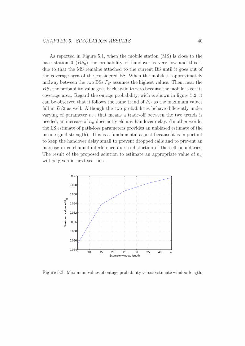
5 10 15 20 25 30 35 40 450.054
0.056
0.058
0.06
0.062
0.064
0.066
0.068
0.07
Estimate window length
Max
imum
val
ues
of P
O
Figure 5.3: Maximum values of outage probability versus estimate window length.

CHAPTER 5. SIMULATION RESULTS 41
5 10 15 20 25 30 35 40 450.08
0.1
0.12
0.14
0.16
0.18
0.2
0.22
0.24
0.26
Estimate window length
Max
imum
val
ues
of P
H
Figure 5.4: Maximum values of handover probability versus estimate window
length.
Figures 5.3 and 5.4 show the trend of the maximum value of the handover
and outage probability, such a value is assumed when the mobile is at same
distance (D/2) from the two base stations.

CHAPTER 5. SIMULATION RESULTS 42
5.2 Estimate Window Length Pareto Opti-
mization Results
In this section we present the result of the solution to the optimization prob-
lem with respect to the estimate window length. The result is obtained by
considering the objective function expressed in (4.1).
0.054 0.056 0.058 0.06 0.062 0.064 0.066 0.068 0.070.08
0.1
0.12
0.14
0.16
0.18
0.2
0.22
0.24
0.26
Outage probability
Han
dove
r P
roba
bilit
y
Figure 5.5: Handover and outage probability evaluate at nw optimum for the
problem having the objective function in (4.6)
The graph shown in figure 5.5 is parameterized with respect to the weight-
ing coefficient α. The probabilities on the axes are evaluated at the optimum
value of the parameter nw wich depends on values of α. High values of han-
dover probability are obteined for α ∼= 0 and low values for α ∼= 1, on the
contrary the outage probability has an opposite trend. In other words it
is possible to choose the appropriate value of the weighting coefficient for
a given value of handover and/or outage probability. Of course α can be
choosen close to zero, for example, if the specific application requires that
the outage probability is more important otherwise it should be choosen close
to one.

CHAPTER 5. SIMULATION RESULTS 43
5.3 Approximations results
In the following we present results of the approximations provided in the
previous chapter to compute handover and outage probability.
5.3.1 First approximation
0 500 1000 1500 20000
0.2
0.4
0.6
0.8
1
1.2
1.4
distance BS0 − MS
Pr
BS
h=0
h=2
h=4
Figure 5.6: Probability of BSs connection versus distance for the first bound
proposed in Section 3.4
As exhibited in Chapter 4 in the first approximation appear the deter-
minant, maximum and minimum eigenvalue of the covariance matrix Σ. By
using this approximation to plot the base station’s probability connection it
results that the error accumulated in each instant time nT yield a value of the
probability higher than one for hysteresis values different by zero (Fig.5.6).
Althought this result does not allow to apply the approximation to solve
optimization problems using high level of the hysteresis margin, it may be
implemented on applications wich make use of low values of the parameter
h because it noticeably reduces the probabilities computing time.

CHAPTER 5. SIMULATION RESULTS 44
5.3.2 Second approximation
This section evaluates the performance of the approximation proposed in
Section 4.2.
0 500 1000 1500 20000
0.01
0.02
0.03
0.04
0.05
0.06
0.07
0.08
distance MS−BS0
Pha
ndov
er
nw
=10, v=40, m=4
h=2h=4h=6h=8
Figure 5.7: Probability of handover versus distance evaluated by using the second
approximation given by equation (3.19) in Chapter 3, with nw = 10
0 500 1000 1500 20000
0.005
0.01
0.015
0.02
0.025
distance MS−BS0
Pha
ndov
er
nw
=40, v=40, m=4
h=2h=4h=6h=8
Figure 5.8: Probability of handover versus distance evaluated by using the second
approximation given by equation (3.19) in Chapter 3, with nw = 40
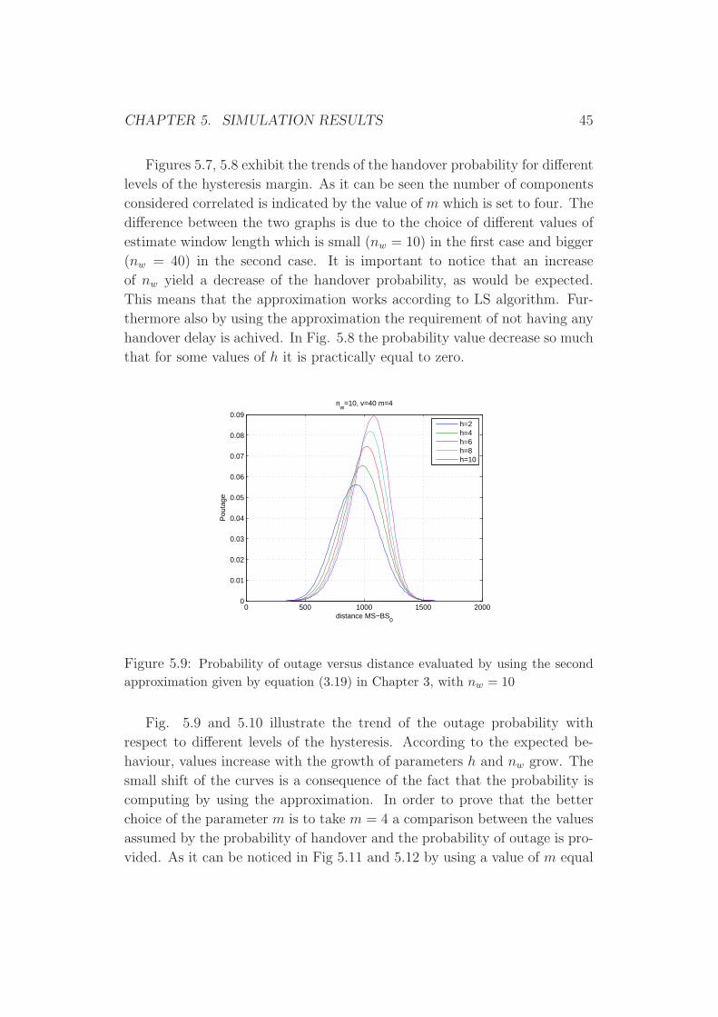
CHAPTER 5. SIMULATION RESULTS 45
Figures 5.7, 5.8 exhibit the trends of the handover probability for different
levels of the hysteresis margin. As it can be seen the number of components
considered correlated is indicated by the value of m which is set to four. The
difference between the two graphs is due to the choice of different values of
estimate window length which is small (nw = 10) in the first case and bigger
(nw = 40) in the second case. It is important to notice that an increase
of nw yield a decrease of the handover probability, as would be expected.
This means that the approximation works according to LS algorithm. Fur-
thermore also by using the approximation the requirement of not having any
handover delay is achived. In Fig. 5.8 the probability value decrease so much
that for some values of h it is practically equal to zero.
0 500 1000 1500 20000
0.01
0.02
0.03
0.04
0.05
0.06
0.07
0.08
0.09
distance MS−BS0
Pou
tage
nw
=10, v=40 m=4
h=2h=4h=6h=8h=10
Figure 5.9: Probability of outage versus distance evaluated by using the second
approximation given by equation (3.19) in Chapter 3, with nw = 10
Fig. 5.9 and 5.10 illustrate the trend of the outage probability with
respect to different levels of the hysteresis. According to the expected be-
haviour, values increase with the growth of parameters h and nw grow. The
small shift of the curves is a consequence of the fact that the probability is
computing by using the approximation. In order to prove that the better
choice of the parameter m is to take m = 4 a comparison between the values
assumed by the probability of handover and the probability of outage is pro-
vided. As it can be noticed in Fig 5.11 and 5.12 by using a value of m equal
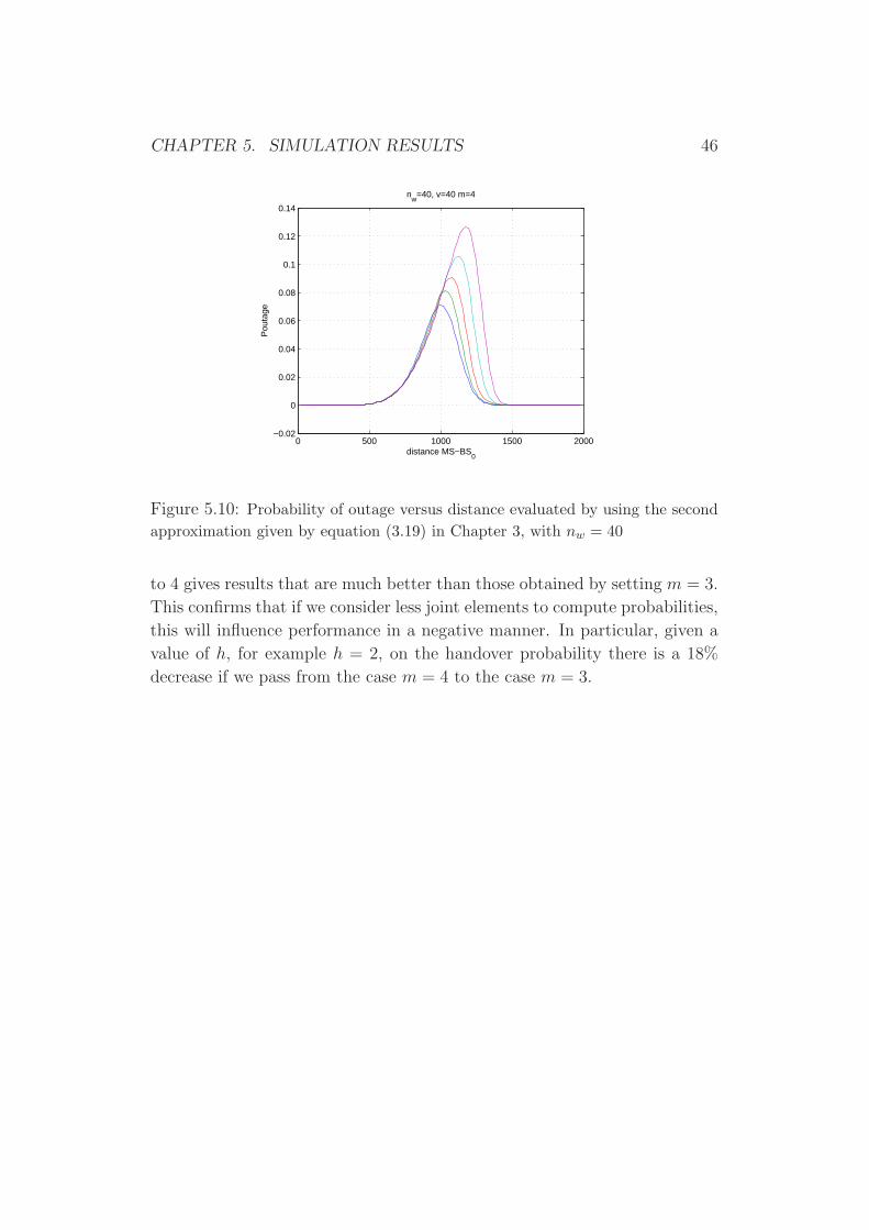
CHAPTER 5. SIMULATION RESULTS 46
0 500 1000 1500 2000−0.02
0
0.02
0.04
0.06
0.08
0.1
0.12
0.14
distance MS−BS0
Pou
tage
nw
=40, v=40 m=4
Figure 5.10: Probability of outage versus distance evaluated by using the second
approximation given by equation (3.19) in Chapter 3, with nw = 40
to 4 gives results that are much better than those obtained by setting m = 3.
This confirms that if we consider less joint elements to compute probabilities,
this will influence performance in a negative manner. In particular, given a
value of h, for example h = 2, on the handover probability there is a 18%
decrease if we pass from the case m = 4 to the case m = 3.

CHAPTER 5. SIMULATION RESULTS 47
0 500 1000 1500 20000
0.01
0.02
0.03
0.04
0.05
0.06
0.07
0.08
distance MS−BS0
Pha
ndov
er
nw
=10, v=40, m=4
h=2h=4h=6h=8
(a) Handover probability for m=4
0 500 1000 1500 20000
0.05
0.1
0.15
0.2
0.25
0.3
0.35
distance MS−BS0
Pha
ndov
er
nw
=10, v=40, m=3
h=2h=4h=6h=8h=10
(b) Handover probability for m=3
Figure 5.11: Comparison between handover probability values for different
m

CHAPTER 5. SIMULATION RESULTS 48
0 500 1000 1500 20000
0.01
0.02
0.03
0.04
0.05
0.06
0.07
0.08
0.09
distance MS−BS0
Pou
tage
nw
=10, v=40 m=4
h=2h=4h=6h=8h=10
(a) Outage probability for m=4
0 500 1000 1500 20000
0.01
0.02
0.03
0.04
0.05
0.06
0.07
0.08
0.09
distance MS−BS0
Pou
tage
nw
=10, v=40, m=4
h=2h=4h=6h=8h=10
(b) Outage probability for m=3
Figure 5.12: Comparison between outage probability values for different m

CHAPTER 5. SIMULATION RESULTS 49
5.4 Performance Evaluation of Hysteresis Op-
timization
The formulation of the minimization problems with respect to the optimum
value of hysteresis margin is developed in Chapter 4. In this section we
investigate both static and dynamic optimization effects on the functions
involved.
5.4.1 Static Optimization Results
In Section 4.7 we introduced the static optimization problem with respect
to the hysteresis margin and formulated an algorithm to find optimum val-
ues of h along the trip of the mobile station (MS). In this subsection we
report results obtained by applying the algorithm to minimize statically the
approximated probabilities.
0
50
100
150
0
0.5
10
0.02
0.04
0.06
0.08
Values of nValues of a
Ph(
a,n,
h* )
Figure 5.13: Handover probability evaluated at optimum h for the static opti-
mization problem.
Fig. 5.13 illustrates the trend of handover probability evaluated in hopt:
decreasing the value of a from 1 to 0 the trend tends to lower values. The
same analysis can be performed for the outage probability in Fig 5.14, even
if it follows an opposite trend with respect to the variation of a and it can be
seen how a deacrease of a yield a weak increase of PO. This does not match

CHAPTER 5. SIMULATION RESULTS 50
0
50
100
150
0
0.5
10
0.02
0.04
0.06
0.08
0.1
Values of nValues of a
Po(
a,n,
h* )
Figure 5.14: Outage probability evaluated at optimum h for the static optimiza-
tion problem.
the trend shown by the probabilities evaluated in nw optimum, in that case,
infact, an increase of a yielded an increase of PO and a decrease of PH . Fig.
5.15 shows the effect achived by applying the minimization on the objective
function: as the value of the weighting coefficient a decreases, the value of F
evaluated in hopt decreases. The reason why F has this trend is due to that
F (h∗) is the waighting sum of PH(h∗) and PO(h∗) and a decrease of PH(h∗) is
much deep compared to the weak increase of PO(h∗). Furthermore, according
to the model, maximum values of F are achived in correspondence to n = 52,
which indicates that the MS is situated at same distance from the current
and the target BS.
To investigate the impact of a static optimization, we show PH , PO and
Fobj plots obtained by fixing a specific value of h. For comparison purposes
first we set h = 2 (this value is suggested in [1]), then we show graphs
obtained by setting h = 8. In the first case, as it can be seen in Fig. 5.18,
PH and PO assume almost same values, hence in the trend of the objective
function in Fig. 5.17 it is not easy to see the weak increase. In second case,
instead, PH and PO have different values and that is why a decrease of a
yield a decrease of cost function. By comparing plot in Fig 5.15 and plot in
Fig. 5.17 it is evident the advantage achived by using the static optimization
technique.

CHAPTER 5. SIMULATION RESULTS 51
0
50
100
150
0
0.5
10
0.02
0.04
0.06
0.08
Values of nValues of a
F(a
,n,h
* )
Figure 5.15: Objective function evaluated at optimum h for the static optimiza-
tion problem.

CHAPTER 5. SIMULATION RESULTS 52
0
50
100
150
0
0.5
10
0.02
0.04
0.06
0.08
Values of nValues of a
Ph(
a,n,
h)
(a) Handover probability
0
50
100
150
0
0.5
10
0.02
0.04
0.06
0.08
Values of nValues of a
Po(
a,n,
h)
(b) Outage probability
Figure 5.16: Handover and Outage probabilities evaluated by setting a fixed
histeresis margin h=2: no optimization
0
50
100
150
0
0.5
10
0.02
0.04
0.06
0.08
Values of nValues of a
F(a
,n,h
)
Figure 5.17: Objective function evaluated by setting h=2: no optimization

CHAPTER 5. SIMULATION RESULTS 53
0
50
100
150
0
0.5
10
0.002
0.004
0.006
0.008
0.01
0.012
Values of n
h=8
Values of a
Ph(
a,n,
h)
(a) Handover probability
0
50
100
150
0
0.5
10
0.02
0.04
0.06
0.08
Values of n
h=8
Values of a
Po(
a,n,
h)
(b) Outage probability
Figure 5.18: Handover and Outage probability evaluated by setting a fixed
histeresis margin h=8: no optimization
0
50
100
150
0
0.5
10
0.02
0.04
0.06
0.08
Values of n
h=8
Values of a
F(a
,n,h
)
Figure 5.19: Objective function evaluated by setting h=8: no optimization

CHAPTER 5. SIMULATION RESULTS 54
5.4.2 Dynamic Optimization Results
The theoretical analysis of an hysteresis dynamic optimization is developed
in previous chapter. In this subsection we evaluate results obtained by Mat-
Lab for the dynamic optimization of handover and outage probabilties. In
this case the optimization is carried out taking into account the influence
of the channel from the current time instant to the next four time instants.
The objective functions are evaluated in a region which is close to the cells
boundaries, so we take into account a path of Dis = 500m, whose left side
is 750 m far from BS0. Notice that if we compare the objective function
obtained by using a dynamic optimization technique, values are lower than
those assumed by applying the static one. In this case we use different values
of the weighting coefficient α which are significant to show that the opti-
mization works well by weighting differently the probabilities involved. In
particular we choose
• α = 0.2, in this case bigger weight is given to the probability of han-
dover;
• α = 0.5, in this case same weight is given to the probabilities;
• α = 0.8, in this case bigger weight is given to the probability of outage;
As shown in Fig. 5.20 and Fig. 5.21 where α = 0.8 and α = 0.5 re-
spectively, by using dynamic optimization, better performance are achived
mostly in the region close to the BS1. When the mobile node is going out
from the coverage area of the BS0 dynamic thecnique works worst and this
is due to that in the middle of the path the recived signal strength varations
are really fast and looking at the future does not improve what the mobile
node knows about the channel. As can be seen in Fig. 5.21 even when the
mobile is close to BS0 the dynamic optimization works better. In the case
of Fig. 5.22 the dynamic technique works better than the static one for each
distance. In this plots the value of the estimate window length nw is setted
to 40.

CHAPTER 5. SIMULATION RESULTS 55
700 800 900 1000 1100 1200 13000.01
0.02
0.03
0.04
0.05
0.06
0.07
distance MN−BS0
Obj
ectiv
func
tion
at h
opt
alpha=0.8
dynamicstatic
Figure 5.20: Comparison between objective functions evaluate at hopt by applying
dynamic and static optimization techniques with a weigthing cofficient equal to
0.5
700 800 900 1000 1100 1200 13000.005
0.01
0.015
0.02
0.025
0.03
0.035
0.04
0.045
distance MN−BS0
Obj
ectiv
e fu
nctio
n at
hop
t
alpha=0.5
dynamicstatic
Figure 5.21: Comparison between objective functions evaluate at hopt by applying
dynamic and static optimization techniques with a weigthing cofficient equal to
0.8

CHAPTER 5. SIMULATION RESULTS 56
700 800 900 1000 1100 1200 13000.002
0.004
0.006
0.008
0.01
0.012
0.014
0.016
0.018
0.02alpha=0.2
distance MN−BS0
Obj
ectiv
e fu
nctio
n at
hop
t
dynamicstatic
Figure 5.22: Comparison between objective functions evaluate at hopt by applying
dynamic and static optimization techniques with a weigthing cofficient equal to
0.2
CHAPTER 5. SIMULATION RESULTS 57
5.4.3 Improving Factors
To show the improvement obtained by applying the optimization methods
proposed in this thesis, in this subsection we show the improving factors
achived by comparing objective functions obtained in the follow cases:
1. fixed level of the hysteresis margin (h = 2) and static optimization;
2. fixed level of the hysteresis margin (h = 2) and dynamic optimization;
3. fixed level of the hysteresis margin (h = 8) and optimization;
4. fixed level of the hysteresis margin (h = 8) and dynamic optimization;
5. static vs dynamic optimization.
Fig. 5.23 shows the improving factor obtained by comparing the objective
function at hopt for the static optimization and the objective function eval-
uated at h = 2 without any optimization. The value of the weighting coef-
ficient is α equal to 0.2. As it is shown there is a drammatic improvement
which is expressed in percentage. Notice that this factor is really high be-
cause the worst case for the objective function is the choice h = 2 as we
assumed in this comparison. The improvement obtained if we compare the
same objective function at h = 2 (no optimization) with the objective func-
tion evaluate at hopt by applying dynamic optimization, is shown in Fig.
5.24. The improvement in this case is even higher than the one obtained
in Fig. 5.23 and this is the proof that dynamic optimization works better
than the static one. As shown in previous sections the choice of h = 2 is
the worst choice among fixed values of the parameter h; this result also in
the improvement that we can obtain by applying optimization methods. Fig.
5.25 shows the improving factor obtained by comparing the objective func-
tion at hopt for the static optimization and the objective function evaluated
at h = 8 without any optimization. The value of the weighting coefficient is
α equal to 0.2. This factor is smaller than the improving factor obtained in
the previous comparison. The same can be observed if we compare objective
function for dynamic optimization with the objective function at h = 8 (Fig.
5.26). The improvement is certainly smaller in the comparison between ob-
jective functions evaluated at hopt for static and dynamic optimization, as
shown in Fig. and this confirms that static optimization works always very
well but the dynamic one is even better.

CHAPTER 5. SIMULATION RESULTS 58
700 800 900 1000 1100 1200 1300200
300
400
500
600
700
800
Impr
ovin
g fa
ctor
(%
)
distance MN−BS0
alpha=0.2
Figure 5.23: Improving factor between objective function evaluated by fixing an
hysteresis margin h = 2 and the objective function at hopt computed by using the
static optimization
700 800 900 1000 1100 1200 1300200
300
400
500
600
700
800
900
1000
distance MN−BS0
Impr
ovin
g fa
ctor
(%
)
alpha=0.2
Figure 5.24: Improving factor between objective function evaluated by fixing an
hysteresis margin h = 2 and the objective function at hopt computed by using the
dynamic optimization

CHAPTER 5. SIMULATION RESULTS 59
700 800 900 1000 1100 1200 130010
15
20
25
30
35
40
45
50
55
60
distance MN−BS0
Impr
ovin
g fa
ctor
(%
)
alpha=0.2
Figure 5.25: Improving factor between objective function evaluated by fixing an
hysteresis margin h = 8 and the objective function at hopt computed by using the
dynamic optimization
700 800 900 1000 1100 1200 130020
40
60
80
100
120
140
distance MN−BS0
Impr
ovin
g fa
ctor
(%
)
alpha=0.2
Figure 5.26: Improving factor between objective function evaluated by fixing an
hysteresis margin h = 8 and the objective function at hopt computed by using the
dynamic optimization

CHAPTER 5. SIMULATION RESULTS 60
700 800 900 1000 1100 1200 13000
20
40
60
80
100
120
distance MN−BS0
Impr
ovin
g fa
ctor
(%
)
alpha=0.2
Figure 5.27: Improving factor between objective function evaluated by using static
and dynamic optimization. The value of the parameter α is 0.2

Chapter 6
Conclusions
The contribution of this thesis regards two aspects. First, to overcome the
limitation due to limited computational resources we studied an approxi-
mation to compute the probability of handover and probability of outage
evaluated along the trip of a mobile station moving between two base sta-
tions. The numerical results show that the approximated probabilities follow
a good behavior. Starting by a well known model, we have then studied some
optimization problems of these probabilities with respect to parameters that
play a crucial role in term of algorithms performance. Without considering
any hysteresis margin we provided an optimization of the estimate window
length which is the number of samples to estimate with a desired accuracy
these probabilities by solving a static minimization problem. We showed that
this optimization allows to choose a fair value of the weighting coefficient and
the choice is based on the considered application. Then we formulated other
two optimization problems with respect to the level of the hysteresis mar-
gin, an important parameter that should be properly choosen to avoid the
so called ping pong effect which is a frequent connection and disconnection
with the same base station by the mobile node. This could be expensive for
the network in terms of traffic load. We proved that by formulating different
optimization problems better performance can be obtained with respect to
existing algorithms. Results show that performance achived by choosing a
fixed value of the hysteresis margin are worst compared to the performance
achived by appling the studied optimizations:
• static optimization outperforms significantly a non optimized handover;
• dynamic optimization outperform the static one at the cost of an in-
61

CHAPTER 6. CONCLUSIONS 62
creased computational complexity.
We can see that static optimization works always very well but the dynamic
one is even better. We obtained drammatic improving factors that show this
results.
Future works
In this thesis we show how the algorithm is sensitive to the variations of
the estimate window length and the level of the hysteresis margin, and we
studied an optimization of the algorithm with respect to these parameters.
However, as the window length and the hysteresis affects differently the in-
volved probabilities, could be useful to do a joint optimization of these two
parameters to choose fair values for both of them.

Bibliography
[1] N. Benvenuto, F. Santucci: A Least Squares Path-Loss Estimation Ap-
proach to Handover Algorithms, IEEE Transaction on Vehicular Tech-
nology, Vol. 48, No. 2, March 1999.
[2] Dimitri P. Bertsekas: Dynamic programming and optimal control.,
Athena scientific, 1995.
[3] Zach Shelby, Carsten Bormann: 6LoWPAN: The Wireless Embedded
Internet. WILEY, 2009.
[4] Carlos J. Bernardos, Antonio De La Oliva, Marıa Calderon, Dirk von
Hugo, and Holger Kahle:NEMO: Network Mobility. Bringing ubiquity
to the Internet access. Demonstration at IEEE INFOCOM 2006, April
2006.
[5] M. Gudmundson: Radio Communication Systems. IEEE Elettronics
Letters, Vol. 27, No. 23, November 1991.
[6] Gordon L. Stuber: Principles of Mobile Communication. Kluwer Aca-
demic Publishers, 1996.
[7] D. Culler, D. Estrin, M. Srivastava: Overview of Sensor Networks, IEEE
Computer Society, August 2004.
[8] A. Murase, I. C. Symington and E. Green: Handover criterion for
macro and microcellular systems, IEEE Vehicular Technology Confer-
ence, Saint Louis, May 1991.
63