Embed Size (px)
Citation preview

Optimization of Oscillating Body for Vortex Induced Vibrations
Project #: BJSWE10
A Major Qualifying Project Report
Submitted to:
Primary WPI Advisor: Brian James Savilonis
in partial fulfillment for the requirements for the
Degree of Bachelor of Science
Submitted by:
________________________ Daniel Distler
________________________ Benjamin Johnson
________________________ Mathew Kielbasa
________________________ Barton Phinney
_____________________________ Professor Brian Savilonis Primary Project Advisor Date: April 28th, 2011

1
ABSTRACT
Energy from vortex induced vibrations harnessed by either wind or water may be a
viable source to generate renewable energy. This report investigates the optimization of
bluff body cross-sectional shapes for vortex creation. Selection began by using finite
element analysis software and comparing the oscillatory lift coefficients of 12 geometric
shapes to a basic cylinder. From these 12 shapes, a “T” shape and a “T” shape with circular
trailing edges were selected to be compared to the cylinder in water tank testing. The
shapes were manufactured using an ABS rapid prototyping machine and tested in a stand
utilizing springs for damping and a fluid flow tank system designed by the team. The
frequencies and displacements were analyzed revealing that the “T” shapes produced 50¿
greater forces and 40% greater amplitudes than the cylinder. However, the cylinder
produced an 85% higher frequency, which resulted in higher total mechanical energy. This
study concluded the “T” shapes should be used for low speed, high torque generators, while
the cylinder should be used for high speed, low torque generators, and the energy
harnessed for electricity would be dependent upon the efficiency of the generator.

2
ACKNOWLEDGEMENT
We would like to extend our thanks to the following individuals and organizations for their
continued support and assistance throughout the duration of our project:
Professor Savilonis for being our project advisor and helping us bring this project to
successful completion
Worcester Polytechnic Institute for providing us with the facilities and resources
necessary for conducting out research.

3
AUTHORSHIP PAGE
The signatures below verify that work relating to this report was completed collectively.
Each section of the final report was completed with the collaboration of all group members
signing below. Daniel Distler, Benjamin Johnson, Mathew Kielbasa, and Barton Phinney
each contributed equal efforts in the research, writing, and editing of the final report.
________________________ Daniel Distler
________________________ Benjamin Johnson
________________________ Mathew Kielbasa
________________________ Barton Phinney
4
TABLE OF CONTENTS
ABSTRACT ............................................................................................................................................................... 1
ACKNOWLEDGEMENT ........................................................................................................................................ 2
AUTHORSHIP PAGE ............................................................................................................................................. 3
TABLE OF CONTENTS ......................................................................................................................................... 4
LIST OF FIGURES ................................................................................................................................................... 8
LIST OF TABLES.................................................................................................................................................. 10
EXECUTIVE SUMMARY .................................................................................................................................... 11
1. Introduction ................................................................................................................................................ 15
2. Background ................................................................................................................................................. 18
2.1. Cause of Vortices ............................................................................................................................... 18
2.2. Vortex Shedding ................................................................................................................................ 19
2.2.1. Von Kármán Vortex Street ........................................................................................................ 21
2.2.2. Different Reynolds Number Regions .................................................................................... 21
2.3. Vortex Induced Vibrations ............................................................................................................ 23
2.3.1. Influence of Vortex Shedding on Vortex Induced Vibrations ...................................... 24
2.4. Different Bluff Body Shapes .......................................................................................................... 26
2.5. Past Research ..................................................................................................................................... 28
2.5.1. Case Study I: University of Michigan .................................................................................... 28
5
2.5.2. Case Study II: California Institute of Technology ............................................................. 30
2.6. Theory and Equations ..................................................................................................................... 30
2.7. Energy in Water ................................................................................................................................ 33
2.8. Positive Environmental Impacts ................................................................................................ 34
3. Design Process ........................................................................................................................................... 36
3.1. Test Tank Design .............................................................................................................................. 36
3.2. Sliding Mechanism/Prototype Design ...................................................................................... 40
3.2.1. Linear Guide/Bearing Sliding Prototype ............................................................................. 40
3.2.2. Horizontally Oscillating Slider Prototype ........................................................................... 43
4. Methodology ............................................................................................................................................... 45
4.1. ANSYS Fluent Testing Methods ................................................................................................... 45
4.2. Test Tank Construction .................................................................................................................. 47
4.2.1. Test Channel ................................................................................................................................... 47
4.2.2. Diffuser ............................................................................................................................................ 48
4.2.3. Oscillation Testing Stand ........................................................................................................... 49
4.2.4. Converger ........................................................................................................................................ 50
4.2.5. Submersible Pumps ..................................................................................................................... 50
4.2.6. Test Tank Setup ............................................................................................................................ 51
Test Equipment Utilized ........................................................................................................................ 51
4.3. Determining the Velocity Profile at the Test Area ............................................................... 53
6
4.4. Oscillation Data Recording............................................................................................................ 55
5. Results and Analysis ................................................................................................................................ 58
5.1 Fluent FEA Trials for Basic Shapes .................................................................................................. 58
5.2 T-Shape Trials ......................................................................................................................................... 66
5.3 Flow Velocity Testing Results ........................................................................................................... 75
5.4 Physical Testing Results ...................................................................................................................... 78
6. Conclusions and Recommendations ................................................................................................. 82
6.1. Conclusions from Computer Simulations................................................................................ 82
6.2. Conclusions from Physical Testing ............................................................................................ 83
6.3. Recommendations for Further Research ................................................................................ 84
BIBLIOGRAPHY ................................................................................................................................................... 88
APPENDIX A: FREQUENCIES FOR VARIOUS LENGTH TO WIDTH RATIOS FOR A T SHAPPED
VORTEXSHEDDER ............................................................................................................................................. 91
APPENDIX B: PROPOSED TANK DESIGN .................................................................................................. 92
APPENDIX C: MATHCAD CALCULATIONS FOR STRESS AND DEFLECTION OF OSCILLATING
RODS ....................................................................................................................................................................... 93
APPENDIX D: FINAL TANK DESIGN ............................................................................................................ 94
APPENDIX E: A TABLE USED IN THE MATERIAL SELECTION PROCESS FOR THE
OSCILLATING RODS .......................................................................................................................................... 95

7
APPENDIX F: A TABLE OF FLOW SPEED RESULTS THAT MAPS THE VELOCITY PROFILE
FOR DIFFERENT PUMP CONFIGURATIONS ............................................................................................ 96
8
LIST OF FIGURES
Figure 1: Schematic of a large wind turbine (U.S. Energy Information Administration) ....... 15
Figure 2: United States Wind Map Diagram (U.S. Energy Information Administration) ....... 16
Figure 3: Von Kármán Vortex Street at increasing Reynolds Numbers (Green, 1995, p. 537)
................................................................................................................................................................................... 21
Figure 4: Regions of fluid flow across a smooth circular cylinder (Dalton, p. 6) ...................... 22
Figure 5: The collapse of the Tacoma Narrows Bridge (Matsumoto, Shirato, Yagi, Shijo,
Fguchi, & Tamaki, 2003) ................................................................................................................................. 24
Figure 6: Setup of tank and cylinders for the University of Michigan study (Vortex Hydro
Energy, 2010) ...................................................................................................................................................... 28
Figure 7: Triangular (left) and T-shaped (right) vortex shedders (Merzkirch, 2005)............ 28
Figure 8: Energy generation unit from the University of Michigan study (Madrigal, 2008) 29
Figure 9: Setup for California Institute of Technology study (Klamo, 2007) ............................. 30
Figure 10: Oval Flow Circular Design ......................................................................................................... 36
Figure 11: A SolidWorks Model of a Preliminary Tank Design ........................................................ 38
Figure 12: The Diffuser ................................................................................................................................... 39
Figure 13: A SolidWorks screen shot shows the T-Shape installed on linear guides .............. 40
Figure 14: Vertical Rod / Linear Bearing Design ................................................................................... 41
Figure 15: Horizontally Oscillating Design with Pump Configuration ......................................... 43
Figure 16: Channel for Test Tank ................................................................................................................ 48
Figure 17: Test Channel for Test Tank ....................................................................................................... 48
Figure 18: Diffuser for Test Tank ................................................................................................................. 48
Figure 19: Setup of the Oscillation Testing Stand ................................................................................. 49
9
Figure 20: Pump Setup and Configurations ............................................................................................. 50
Figure 21: Secured Setup of Tank Elements ............................................................................................ 51
Figure 22: From Left to Right: Vernier LabPro, Flow Rate Sensor, and Motion Detector. .... 52
Figure 23: Pump Arrangement with Pumps Labeled (CAD Model and Prototype) ................ 53
Figure 24: Velocity Profile Locations and Nomenclature ................................................................... 54
Figure 25: Setup for Velocity Profile Testing .......................................................................................... 54
Figure 26: The Oscillating Test Stand Assembly .................................................................................. 55
Figure 27: Motion Detection Test Setup Picture ................................................................................... 56
Figure 28: Oscillation Measurement (Action Shot) ............................................................................. 57
Figure 29: Overview of Basic Shapes ......................................................................................................... 59
Figure 30: Front Triangle Fluent Results .................................................................................................. 60
Figure 31: Square Fluent Results ................................................................................................................. 61
Figure 32: Ellipse L/W = 0.25 Fluent Results ......................................................................................... 62
Figure 33: Ellipse L/W = 2 Fluent Results ................................................................................................ 63
Figure 34: Circle Fluent Results ................................................................................................................... 64
Figure 35: T-Shape Fluent Results .............................................................................................................. 65
Figure 36: Summarized Results of Basic Shapes from Fluent Testing .......................................... 66
Figure 37: T-Shapes .......................................................................................................................................... 67
Figure 38: Cylindrical T-Shape Fluent Results ....................................................................................... 68
Figure 39: Triangle T-Shape Fluent Results ............................................................................................ 69
Figure 40: Y-T-Shape Fluent Results .......................................................................................................... 70
Figure 41: Parachute T-Shape Fluent Results ......................................................................................... 71
Figure 42: Concave T-Shape Fluent Results ............................................................................................ 72

10
Figure 43: Summary of T-Shape Fluent Testing .................................................................................... 73
Figure 44: Summary of Four Best Performing T-Shapes at Higher Reynold's Numbers ....... 74
Figure 45: Various T-Shapes at Operating Conditions ........................................................................ 75
Figure 46: Velocity Profile Line Sketch of 1/3 hp pump (Left), 1/2 hp pump (center), and
5/6 hp pump (right).......................................................................................................................................... 77
Figure 47: Velocity Profile Isometric View (1/3 HP) ........................................................................... 77
Figure 48: Amplitude Results from Physical Testing ........................................................................... 78
Figure 49: Frequency Results from Physical Testing ........................................................................... 79
LIST OF TABLES
Table 1: Regions of fluid flow across a smooth circular cylinder (Green, 1995, p. 536) ........ 23
Table 2: Average Flow Velocities for Different Pumps in Use .......................................................... 76

11
EXECUTIVE SUMMARY
The purpose of this project was to maximize the hypothetical energy that could be
harnessed from vortex induced vibrations as a form of alternative energy. The objective
was to maximize the displacement amplitudes that are produced by a bluff body, which is
oscillating as a result of the induced vibrations. This was done by experimenting with the
cross-sectional shape of the bluff body. It was hypothesized that obtaining larger
amplitudes would result in a larger amount of work done on a generator, which would
result in more energy that could be harnessed to produce electricity. Under this
assumption, the shape that produced the largest amplitudes would hypothetically produce
the largest amount of energy. Traditionally, a circular shape (i.e. cylinder) is used in flow
models to demonstrate vortices, and therefore, it was used as a control for the experiments.
The study started by using FEA analysis to determine which shapes would generate the
largest lift coefficient. This parameter would provide the largest lift forces and, in theory,
the largest amplitudes. From these shapes, three were selected to be manufactured for
physical testing in a specially made, small scale test tank.
In order to determine which shapes would produce the largest lift coefficients, FEA
tests using Ansys Fluent were conducted using a variety of basic shapes, such as a circle,
square, triangle, T-shape, and ellipse, to narrow down to one shape that would be
experimented with. These tests were conducted using a Reynold’s number range from 100-
5000. From the basic shapes, it was found that the T-shape produced the largest lift
coefficient, and it was selected to be experimented with for different variations of the
shape, such as a circular-T, triangular-T, parachute-T, Y-T and a concave-T. From the FEA

12
tests with these shapes, which were again conducted with a Reynold’s number range from
100-5000, it was found that the concave-T shape produced the largest lift-coefficient.
Therefore, this shape was selected to be manufactured for the physical testing. The basic T-
shape was also selected as a comparison, and the circle was selected as a control.
The three shapes mentioned above were manufactured in bars out of ABS plastic
using rapid prototyping. The bars were approximately ten inches long and the
characteristic length (i.e. the diameter) was one inch. The bars were vertically attached to a
drawer slider which would allow the bars to oscillate due the vortices they produced.
Springs were attached to the bars to damp the oscillations and allow for damped driven
oscillations. The slider was attached to a piece of plywood that was the approximate width
of the channel of the test tank. The test tank consisted of an oval metal tank that was six
feet long by two feet tall by two feet wide. A flow channel was constructed that was
approximately a foot wide by a foot tall by four feet long. The channel was placed in the
center of the tank with approximately six inches on either side. At one end of the tank,
three sump pumps were placed: two pumps of one half horsepower and one of one third
horse power. The outlet of each one half horse power pump was directed on the outside of
each side of the channel, while the outlet of the one third horsepower pump was split
equally on either side of the channel using PVC pipe. A converger was put at the other end
of the tank, which converged the flows on the outside of channel and redirected them
inside the channel. This created a circular flow in which the flow traveled around the
outside of the channel and then through the middle of the channel.

13
By using the three pumps, three different speeds were used to test the three vertical
bars. The bars were submerged in just under a foot of water in the test tank. The concave-T
had the largest amplitudes and forces of the three shapes, while the T-shape had the second
largest amplitudes and forces. The circle had the smallest amplitudes and forces, which
were much smaller than the other two shapes. It also failed to constantly oscillate, which
may have been due to an inability to obtain the proper lock-in frequency as a result of the
springs used for damping. The concave-T had the smallest frequency, and the T-shape had
the second smallest frequency. The circle had a much larger frequency than the other two
shapes, and because of this feature, it was determined the circle had the highest power
density. However, it is difficult to say which shape would perform better for power
production since the T-shapes could produce more power per period given the high forces
and amplitudes, while the circle could produce more power over time given its shorter
period.
Further work in this area should include research into increasing the scale of
testing, and achieving the lock-in frequency for all test pieces. These changes will increase
the validity of the data collected and may lead to more conclusive paths to continue work.
One additional recommendation for future studies in this area is to consider the type of
generator being used to extract power from the system. The properties of the generator
will highly influence the optimal design of the oscillating body. Energy generation from
vortex induced vibrations had tremendous potential if continued investigations optimize
both the shape of the oscillating body and the efficiency of the entire system when
including the generator.

14

15
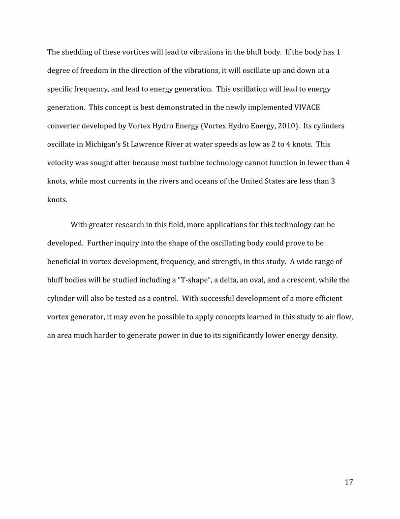
Figure 1: Schematic of a large wind turbine (U.S.
Energy Information Administration)
1. Introduction
As the earth’s population increases and becomes more modernized, it has become
evident that supplying energy to everyone is a daunting task. Furthermore, the resources
used to supply this energy, generally fossil fuels, do not regenerate at a rate to consider
them renewable. The United States gets approximately 93% of its energy from
nonrenewable sources. These sources include uranium ore (nuclear), coal, natural gas, and
oil (U.S. Energy Information Administration). As we drain the supplies of earth’s resources,
we must figure out a way to create energy using renewable sources. In recent years,
interest has been shown in the field of renewable energy generation using sources such as
solar panels, hydroelectric dams, hydrogen fuel cells, biofuels, and arguably the most well-
known, wind turbines.
“In 2009, wind machines in
the United States generated a total
of about 71 billion kilowatt-hours,
about 1.8% of total U.S. electricity
generation.” (U.S. Energy
Information Administration)
Wind turbines are a renewable
energy source that requires the
flow of a fluid over its blades. As
wind, the fluid, flows over the blades of a turbine, an airfoil profile incorporated into the
blade will generate lift which spins the blade. The blade is attached to a turbine and
16
generator so the torque that the blade rotation creates leads to the energy generation.
Wind is a source that cannot be depleted. Figure 1 shows the basic components of a large
wind turbine. The driving mechanism for wind is the sun. As long as the sun shines, the
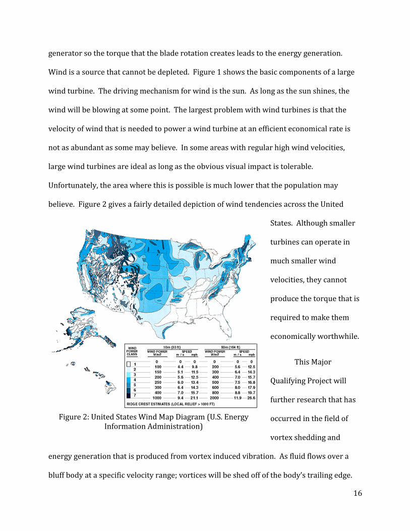
wind will be blowing at some point. The largest problem with wind turbines is that the
velocity of wind that is needed to power a wind turbine at an efficient economical rate is
not as abundant as some may believe. In some areas with regular high wind velocities,
large wind turbines are ideal as long as the obvious visual impact is tolerable.
Unfortunately, the area where this is possible is much lower that the population may
believe. Figure 2 gives a fairly detailed depiction of wind tendencies across the United
States. Although smaller
turbines can operate in
much smaller wind
velocities, they cannot
produce the torque that is
required to make them
economically worthwhile.
This Major
Qualifying Project will
further research that has
occurred in the field of
vortex shedding and
energy generation that is produced from vortex induced vibration. As fluid flows over a
bluff body at a specific velocity range; vortices will be shed off of the body’s trailing edge.
Figure 2: United States Wind Map Diagram (U.S. Energy
Information Administration)
17
The shedding of these vortices will lead to vibrations in the bluff body. If the body has 1
degree of freedom in the direction of the vibrations, it will oscillate up and down at a
specific frequency, and lead to energy generation. This oscillation will lead to energy
generation. This concept is best demonstrated in the newly implemented VIVACE
converter developed by Vortex Hydro Energy (Vortex Hydro Energy, 2010). Its cylinders
oscillate in Michigan’s St Lawrence River at water speeds as low as 2 to 4 knots. This
velocity was sought after because most turbine technology cannot function in fewer than 4
knots, while most currents in the rivers and oceans of the United States are less than 3
knots.
With greater research in this field, more applications for this technology can be
developed. Further inquiry into the shape of the oscillating body could prove to be
beneficial in vortex development, frequency, and strength, in this study. A wide range of
bluff bodies will be studied including a “T-shape”, a delta, an oval, and a crescent, while the
cylinder will also be tested as a control. With successful development of a more efficient
vortex generator, it may even be possible to apply concepts learned in this study to air flow,
an area much harder to generate power in due to its significantly lower energy density.
18
2. Background
In order to fully understand the principle of generating energy through vortex
induced vibrations, there must be a deeper understanding of the forces involved. This
background will introduce vortices, their causes, their behavior in varying fluid flow, and
the repercussions of vortex generation. Past research in the field of vortex induced
vibrations will be discussed. Finally, the positive environmental impacts of this type of
energy generation and the available energy in water will be examined.
2.1. Cause of Vortices
All real fluids have a shear viscosity that is greater than zero, and a fluid with a
shear viscosity of zero is an idealized fluid used for simplifying calculations. Since all fluids
possess some shear viscosity, as a fluid flows over a rigid body, a boundary layer of fluid is
created at the surface of the body (Wu, Ma, & Zhou, 2006, p. 2). A boundary layer can be
defined as a “thin layer of fluid adjacent to the surface of the structure through which the
flow velocity increases from 0 at the surface to the free stream velocity at the outer edge of
the boundary layer.” (Green, 1995, p. 534). Shear stresses are a result of these boundary
layers, which cause a rotational flow where the boundary layer separates from the rigid
body. These rotational flows are what make up vortices, and have a very high
concentration of energy. Given certain Reynolds numbers, the concentrated vortices will
interact with one another, becoming unstable and create turbulence (Wu, Ma, & Zhou,
2006, p. 2).
Vortices can be categorized by 3 separate types. These types include forced (or
rotational) vortices, free (or irrotational) vortices, and combined vortices (Wu, Ma, & Zhou,
19
2006, pp. 302 - 303). Forced vortices occur when a liquid tank is spun around its central
axis. When this occurs at a certain angular velocity, the tangential velocity of the rotating
fluid is proportional to the distance from the central axis (vortex’s core). In this case, the
rotating fluid can be looked at as a rigid body rotating about its central axis. The speed of
the fluid at the center of vortices of this type will be zero.
The next type of vortex that exists is a free or irrotational vortex (Wu, Ma, & Zhou,
2006, pp. 302 - 303). These are most commonly seen when draining a sink or bathtub. For
this type of vortex, the tangential velocity of the fluid is inversely proportional to the
distance from the axis of rotation. Fluid farther from the vortex core will be rotating
slower than that nearer to the core. For free vortices, the angular velocity is greatest at the
center.
Combined vortices often form naturally. A combined vortex consists of a forced
vortex ‘trapped’ inside of a free or irritation vortex (Wu, Ma, & Zhou, 2006, pp. 302 - 303).
The center part of the vortex is behaving as a forced vortex, but the ‘tank’ that it is within is
a free vortex. This spinning free vortex causes the inner part to spin and therefore it acts as
a forces vortex.
2.2. Vortex Shedding
Vortex shedding is determined by two properties; the viscosity of the fluid passing
over a bluff body, and the Reynolds number of that fluid flow. The Reynolds number
relates inertial forces to the viscous forces of fluid flow (Water Flow in Tubes - Reynolds
Number). In higher Reynolds number regions, inertial forces dominate the flow and
turbulence is found, while in low Reynolds number regions, viscous forces dominate the
20
flow and laminar flow is developed. The creation of strong clean vortices occurs in lower
Reynolds number regions. When flow separates from the trailing edge of a submerged
body, a region of extreme low pressure will occur because of viscous effects (Georgia Tech).
A vortex will form in this area of extreme low pressure to create pressure equilibrium. As
fluid flow over the bluff body continues, disturbances will cause the vortex to be “shed”
from the trailing edge of the submerged body. Again, a low pressure region will be created
and the previous process will continue.
“Vortex shedding can induce damaging large amplitude vibrations of flexible
structures in fluid flows and produce intense acoustic pressures in ducts.” (Green, 1995, p.
533). The frequency of vortex shedding is a function of the Strouhal number which relates
the frequency to the free stream velocity and cylinder diameter (Georgia Tech). Through
testing it has been accepted that the Strouhal number is 2.1 for a wide range of Reynolds
number, for infinitely long circular cylinders. The fact that the Strouhal number is so
consistent allows the frequency of vortex shedding to be used as the basis for the design of
fluid flow meters (Green, 1995, p. 541).
At higher Reynolds numbers, vortex shedding varies over a narrow band of
frequencies, with varying amplitudes, and also varies along the span of a submerged,
stationary cylinder (Green, 1995, p. 541). Pressure oscillations that occur in Reynolds
numbers under 400 tend to be the strongest (Georgia Tech). The strong oscillations lead to
the formation of a Kármán Vortex Street. Reynolds numbers greater than 400 entail street
destruction due to turbulence. This meaning the flow will not be straight, and there will be
disruptions in the flow.

21
2.2.1. Von Kármán Vortex Street
A von Kármán vortex street is the description given to an alternating pattern of
vortices. When a fluid flows over a blunt, 2 dimensional body, vortices are created and
shed in an alternating fashion on the top and bottom of the body (Graebel, 2007, p. 103).
Given that the body is symmetrical, this phenomenon will initially be symmetrical but will
eventually turn into the classical alternating pattern. Figure 3 is a good depiction of a
common von Kármán vortex street. This behavior was named after Theodore Von Kármán
for his studies in the field.
“Although von Karman’s (1912) ideal
vortex street has been long associated with
the wake of a circular cylinder, the only
requirement for the existence of a vortex
street is two parallel free shear layers of
opposite circulation which are separated by
a distance h.” (Green, 1995, p. 536). Von
Karman calculated that in order for there to be stability in the Karman vortex street, the
ration between the vertical distance between the centers of alternating vortices, h, and the
horizontal distance between the centers of alternating vortices, l, ideally should be
approximately 0.281.
2.2.2. Different Reynolds Number Regions
Figure 3: Von Kármán Vortex Street at increasing Reynolds Numbers (Green,
1995, p. 537)

22
The behavior of a how a fluid will flow around a rigid object can be related to the
Reynolds Number of the fluid flow. The Reynolds number is a unit without dimensions that
measures the ratio between inertial forces and viscous forces (Dalton, p. 6). Inertial forces
(also known as fictitious forces) are defined in accelerated frames. These frames include
straight line (or rectilinear) acceleration, rotational (centrifugal or Coriolis) accelerations,
and the fourth is from a changing angular velocity. Viscous forces are dependent on the
fluid and temperature. When viscous
forces are relatively high, the
viscosity is said to be high, denoting a
relatively “thick” fluid. For different
values of Reynolds numbers, a fluid
will flow differently about a rigid
body. From previous studies of
vortices created behind a cylinder
placed in a fluid flow, the following
ranges of Reynolds numbers proved
to result in the vortices shown in
Figure 4.
The flow patterns observed for different ranges of Reynolds numbers from another
study are shown in Table 1 below.
Figure 4: Regions of fluid flow across a smooth
circular cylinder (Dalton, p. 6)

23
Table 1: Regions of fluid flow across a smooth circular cylinder (Green, 1995, p. 536) Reynolds Number
Range: Flow Observations:
0<Re<5 Flow follows cylinder contours (no vortices). 5<Re<45 Flow creates a symmetric pair of vortices. As Re increases in this
region, the stream wise length of the vortices will increase up to 3*d at 45)
Re>45 Flow creates laminar periodic vortex street.
150<Re<300 Shed vortices become turbulent, Boundary layer along cylinder remains laminar
300<Re<3x10⁵ Vortex street is fully turbulent 3x10⁵<Re<3.5x10⁶ Laminar Boundary Layer has undergone turbulent transition.
Wake is narrower and disorganized
3.5x10⁶<Re Re-establishment of turbulent vortex street
These two studies returned very similar results. The first study gives more detail
for the fluid flow in the range of Reynolds numbers from 45 to 150.
2.3. Vortex Induced Vibrations
Vortex induced vibrations occur when the shedding of vortices occurs, alternating
on either side of a bluff body. The repeated, alternating shedding of vortices creates a force
that is normal to the general direction of flow over the bluff body. This load will alternate,
corresponding to the side each vortex is shed from (Hansen, 2007). When the load varies
in a harmonic manner at the same frequency as the vortex, vibrations will occur and
become stronger. This frequency is a function of the Strouhal number.
24
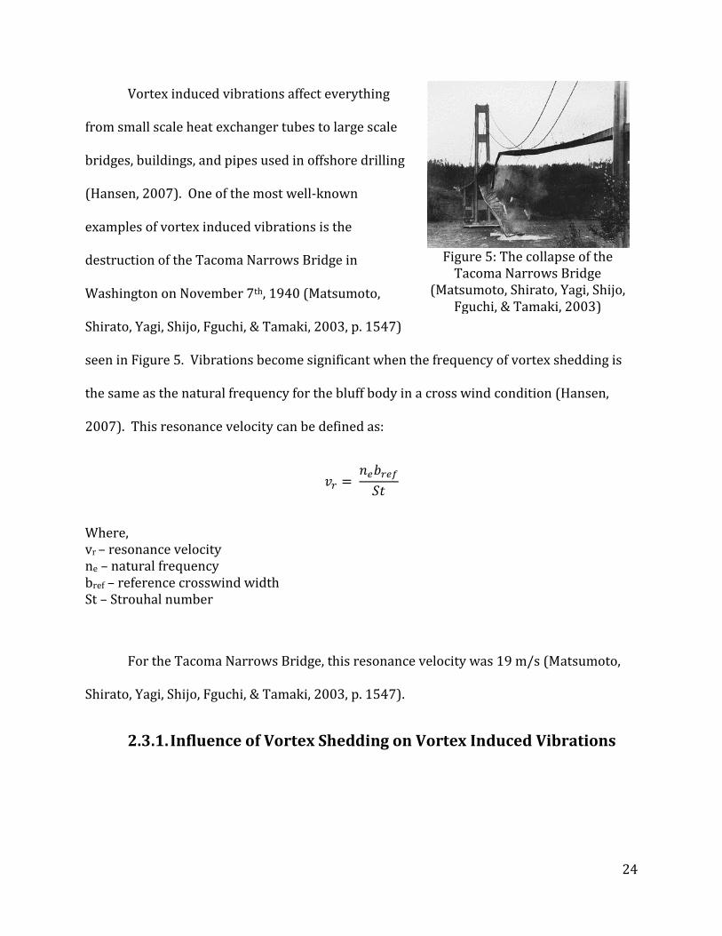
Figure 5: The collapse of the
Tacoma Narrows Bridge (Matsumoto, Shirato, Yagi, Shijo,
Fguchi, & Tamaki, 2003)
Vortex induced vibrations affect everything
from small scale heat exchanger tubes to large scale
bridges, buildings, and pipes used in offshore drilling
(Hansen, 2007). One of the most well-known
examples of vortex induced vibrations is the
destruction of the Tacoma Narrows Bridge in
Washington on November 7th, 1940 (Matsumoto,
Shirato, Yagi, Shijo, Fguchi, & Tamaki, 2003, p. 1547)
seen in Figure 5. Vibrations become significant when the frequency of vortex shedding is
the same as the natural frequency for the bluff body in a cross wind condition (Hansen,
2007). This resonance velocity can be defined as:
Where, vr – resonance velocity ne – natural frequency bref – reference crosswind width St – Strouhal number
For the Tacoma Narrows Bridge, this resonance velocity was 19 m/s (Matsumoto,
Shirato, Yagi, Shijo, Fguchi, & Tamaki, 2003, p. 1547).
2.3.1. Influence of Vortex Shedding on Vortex Induced Vibrations

25
Due to vortex shedding essentially being a sinusoidal process, it is possible to model
the lift from vortex induced vibrations as a force that oscillates harmonically (Green, 1995,
p. 546). This force can be described as:
Where, FL –> Force of vortex induced lift ρ –> fluid density U –> free stream velocity D –> diameter or characteristic length CL –> lift coefficient ωs = 2πfs –> circular vortex shedding frequency t - > time fs -> vortex shedding frequency
When a submerged cylinder vibrates normal to the free stream direction at the
vortex shedding frequency, or relatively close, the vibrations can cause four main reactions
(Green, 1995, p. 542) First, the strength of the shed vortices increase, altering the phase,
sequence and pattern of vortices in the wake. Secondly, the wake may become more
correlated across the span of the bluff body. The third reaction is that the average drag
may increase.
The fourth reaction is more significant. As the frequency of the vortex shedding
becomes closer to the cylinder’s vibration frequency, “lock-in” or “synchronization” occurs
(Green, 1995, p. 542). The “lock-in band” is the range of frequencies where the vortex
shedding frequency is controlled by the vibration frequency of the cylinder. As flow is
adjusted so that the shedding frequency approaches the natural frequency; the vortex
shedding frequency will “lock” onto the structure’s natural frequency. This will lead to

26
produce vibrations in the structure (Green, 1995, p. 545). When the vortex wake oscillates
in a resonating fashion, significant amounts of energy will be applied to the structure. The
range of velocities that will produce this phenomenon can be described as:
Where, U = free stream velocity of fluid fn = natural frequency D = diameter or characteristic length
This can also occur if the cylinder’s frequency of vibration is a multiple or sub-
multiple of the frequency of vortex shedding (Green, 1995, p. 542). Additionally,
submerged cylinders are not the only bluff body shapes where “lock-in” occurs.
2.4. Different Bluff Body Shapes
The shape of the bluff body in a stream determines how efficiently it will form
vortices. This efficiency primarily depends on how easily vortices are generated, how big
they are, and how large the frequency is, which is determined by the Strouhal number (El
Wahed, Johnson, & Sproston, 1993). A study was performed in the early 1990’s by the
University of Liverpool to analyze the effect that different shaped bluff have on vortex
shedding. The purpose of the study was to optimize the performance of flow meters by
designing a bluff body which generates vortices over a wide variety of Reynolds numbers.
The study used five cylinders with different cross sections: circular, trapezoidal, triangular,
rectangular, and T-shaped. The study then tested the cylinders with a computer simulation
program in a flow with a Reynolds number of around 9125. Of the five cylinders tested, the

27
T-Shape cylinder produced the strongest vortices. The study concluded that this was due to
the “splitter plate” of the T-Shape that helped create a clear signal.
A patent for a T-shaped flow meter also provides data on frequencies and
oscillations with respect to the ration of length to width. When this ratio is equal to zero,
the frequency is unstable and keeps changing for all Reynolds numbers between 2,000 and
35000 (Chou, Miau, Yang, & Chen, 1994). This instability remains the case until the ratio
reaches 1.56. At this ratio, steady oscillations occur up until a ratio of 2.0 with the
frequency being larger closest to the ratio value of 1.56. After a ratio of 2.0, the oscillations
become unstable again. However, the magnitude of the frequency decreases as the
length/width ratio increases.
Another such study focused on just a triangle shape and a T-shape, but also reversed
the flow such that the point of each object faced into the flow (Merzkirch, 2005). The study
used a flow varying from 2 m/s to 30 m/s which resulted in Reynolds’s numbers from
13,000 to 195,000. The width of the triangle bluff body was 24 mm, while the width of the
T-shaped body was 10 mm. With the flat side of the triangle into the flow, the frequency
that was produced was 6.7 Hz and a Strouhal number of .16, while with the tip into the flow
produced a frequency of 14 Hz and a Strouhal number of .34. With the flat side of the T-
shape into the flow, the frequency that was produced was 12 Hz and a Strouhal number of
.12, while with the tip into the flow produced a frequency of 20 Hz and a Strouhal number
of .2. Scaling the T-shape down to the size of the triangular shedder, the frequencies
obtained for the flat edge into the flow and the point into the flow are 5 Hz and 8.3 Hz,
respectively. This means that the triangular shape with the point into the flow would
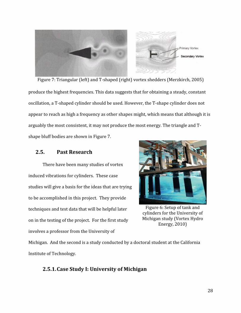
28
Figure 7: Triangular (left) and T-shaped (right) vortex shedders (Merzkirch, 2005)
produce the highest frequencies. This data suggests that for obtaining a steady, constant
oscillation, a T-shaped cylinder should be used. However, the T-shape cylinder does not
appear to reach as high a frequency as other shapes might, which means that although it is
arguably the most consistent, it may not produce the most energy. The triangle and T-
shape bluff bodies are shown in Figure 7.
2.5. Past Research
There have been many studies of vortex
induced vibrations for cylinders. These case
studies will give a basis for the ideas that are trying
to be accomplished in this project. They provide
techniques and test data that will be helpful later
on in the testing of the project. For the first study
involves a professor from the University of
Michigan. And the second is a study conducted by a doctoral student at the California
Institute of Technology.
2.5.1. Case Study I: University of Michigan
Figure 6: Setup of tank and
cylinders for the University of Michigan study (Vortex Hydro
Energy, 2010)

29
The study conducted was done by Professor Michael Bernitsas, who is head of the
Marine Renewable Energy Lab at the University of Michigan at Ann Arbor, and three other
doctorate students (Bernitas, Raghavan, Ben-Simon, & Garcia, 2008). The study conducted
was for high Reynolds Number around 1,000,000. The experiment was performed in a
large tank, and four cylinders were immersed in the tank. Each cylinder was 36 inches in
length and 3.5 inches in diameter. The Test tank can be seen in Figure 6.
The fluid velocity created was 2.6 knots, which is about 1.3 meters per second
(Bernitas, Raghavan, Ben-Simon, & Garcia, 2008). The cylinders are attached to springs
which allow them to move up and down freely, from the current. The springs had a
stiffness value of 518 N/m. The Reynolds Number for the test ranged from 0.44 x 10⁵ to
1.33 x 10⁵. A rotary electrical generator was used to convert the energy harnessed into
electricity. The experimental results were not available. However, Professor Bernitsas
wrote that the system worked as expected and the energy was harnessed and converted
using the electrical converter. Figure 8
shows the setup of the generator, and how it
was setup in order to convert the energy
into electricity.
Professor Bernitsas has also
developed a company around this concept
called Vortex Hydro Energy. They are in the
process of doing large scale testing, in actual
under water environment in the Detroit River. This is expected to be done within the year.
Figure 8: Energy generation unit from
the University of Michigan study (Madrigal, 2008)

30
2.5.2. Case Study II: California Institute of Technology
This system was setup differently than the University of Michigan study and was
used for finding the effects of damping and Reynolds number on vortex induced vibrations
(Klamo, 2007). The setup used was for
much smaller scale testing, and was
elastically-mounted rigid circular
cylinder, free to oscillate only transverse
to the flow direction, with very low
inherent damping. A magnetic eddy-
current damping system was installed to
be able to limit the damping effects. The
range of Reynolds Number used was
between 200 < Re < 5050. Figure 9 shows the experimental setup used. The flow velocities
were varied, and the data was recorded by using a LabView program. For a system with
low mass the system proved to have a constant frequency. As the Reynolds Number
increased the frequency was not consistent.
2.6. Theory and Equations
The theory used for this project is based on flow past a circular cylinder. As the flow
moves across the cylinder, it is lifted because of the lift force, which creates the vortex. The
equation for the lift force for a non-rotating cylinder is:
Figure 9: Setup for California Institute of
Technology study (Klamo, 2007)

31
Where: FL = Lift Force CL = Coefficient of Lift ρ = Density of the fluid D = Diameter or characteristic length l = Length of cylinder U = Fluid Velocity
The drag force is also an important factor in determining the most efficient sliding
design mechanism. The drag force will come from the current of the water and act as the
normal force when finding the frictional force. The drag force can be represented by the
following equation:
Where: CD = Coefficient of Drag FD = Force of Drag
The lift force, above, is dependent on the Reynolds Number. The Reynolds Number
gives a relationship between the density, velocity of fluid, diameter of cylinder, and the
viscosity of the cylinder.
The Reynolds Number can be calculated by the following equation:
32
Where: Re = Reynolds Number µ = Viscosity of Fluid DH = Hydraulic Diameter
An equation for the coefficients was first derived, and then used to solve for the drag
and lift forces, using the Reynolds Number.
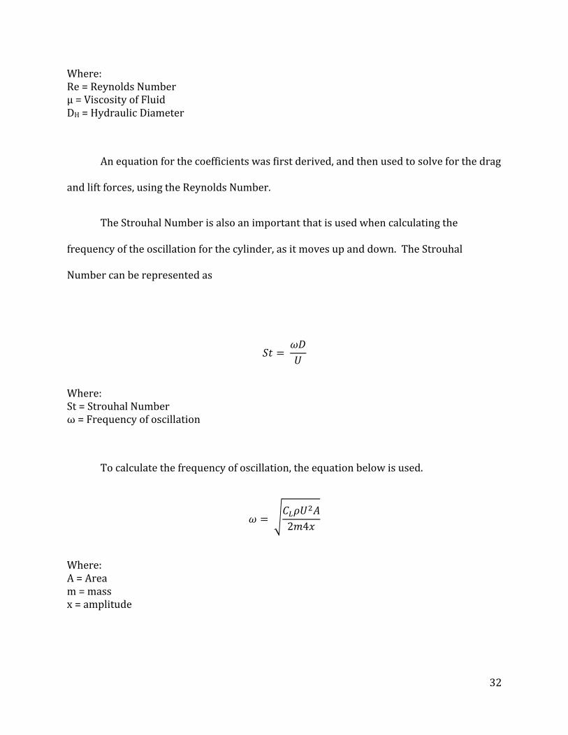
The Strouhal Number is also an important that is used when calculating the
frequency of the oscillation for the cylinder, as it moves up and down. The Strouhal
Number can be represented as
Where: St = Strouhal Number ω = Frequency of oscillation
To calculate the frequency of oscillation, the equation below is used.
√
Where: A = Area m = mass x = amplitude
33
These are the main equations behind the theory of the vortex induced by vibrations
(White, 2011). They will be used in the design phase more to calculate the lift and the
frequency for a given velocity. The velocities used will be used to demonstrate flow from a
current in a natural body of water, such as a river. From here the Strouhal number can
then be compared to the Reynolds number and see the how the two are affected.
2.7. Energy in Water
The amount of energy able to be harnessed in flowing water can be calculated using
the equation for conservation of energy. If heat transfer is neglected and the flow of the
water is assumed to be perpendicular to the control volume such that the full amount of
energy can be calculated, the resulting equation is as follows:
[(ȗ + (ρ/P )+ (V²/2) + gz)ṁ]out – [(ȗ + (ρ/P) + (V²/2) + gz)ṁ]in = Ẇ
Where: ȗ = enthalpy ρ = density P = pressure V = velocity of the water g = acceleration due to gravity z = vertical height ṁ = mass flow rate Ẇ = Power
In order to calculate the amount of usable energy, the energy equation must be
simplified to look at the kinetic energy of the water. This is accomplished by neglecting
changes in enthalpy, pressure, and height, which reduces the equation to:
(V²/2)ṁ = Ẇ

34
However, this power is not the amount of electrical power that can be generated as
no generator is a hundred percent efficient. This power must be multiplied by the efficiency
of a generator to estimate the total amount of electrical power that may be captured. This
equation does not include head loss due to friction since it is for a large body of water
where frictional effects may be considered negligible, along with the efficiency of the
system.
Today, there are many designs that are used to harness water energy as form of
green energy. Most of these devices are turbines that either harness energy from damming
a river to increase potential energy or harness energy from natural tides or ocean currents.
One issue with these devices is that they require large velocity (around 6 knots) in order to
produce useful electricity (Madrigal, 2008). Usually to achieve this flow or more, rivers
need be dammed which has a large negative impact on the environment. The largest
limitation for tidal energy is the fact that most ocean currents only reach speeds of 3 knots,
so areas that have enough flow to justify a tidal generator are scarce (Madrigal, 2008).
However, the amount of energy that can be harnessed in either prevailing currents or tidal
fluctuations is estimated to be between 280,000 and 700,000 terawatt-hours, which is very
large when compared to the worldwide electrical generation figure of 16,000 terawatt-
hours (Vortex Hydro Energy, 2010). Needless to say, there is a lot of potential for
harnessing water energy.
2.8. Positive Environmental Impacts
Current vortex energy projects are able to generate electricity in flows between 2
and 4 knots (Vortex Hydro Energy, 2010). Given that this is about half the flow needed by

35
conventional hydroelectric devices, not only is there a greater energy market, but it does
not require the damming of rivers. Damming rivers can have an extreme negative impact
to the surrounding environment. The area above the dam is completely flooded resulting
in a loss of habitat and the area below the dam is starved for water. Damming significantly
reduces the environmental benefit of using hydro power. Since current devices do not
require damming of rivers, they are very environmentally friendly. They also use
renewably energy, have no emissions, and are relatively small compared to conventional
hydro generators meaning they are unobtrusive to aquatic life. Fish use the vortices to
propel themselves forward and be able to swim in schools.

36
3. Design Process
3.1. Test Tank Design
Designing the test tank took presented many challenges. The main goal that proved
difficult to accomplish was to achieve an even flow profile. The design that we finally
choose to build uses two circular flows of water, merging together into a diffuser, followed
by the testing area.
Preliminary designs included using a single oval or circular-shaped flow channel.
Figure 10 below is a preliminary sketch of this single oval-shaped flow design estimated to
cost $150.
Figure 10: Oval Flow Circular Design
After farther research, the team realized that this design would result in faster flow
velocities on the outer perimeter of the circular flow and slower flow velocities at the inner
perimeter. Since a relatively even flow profile was desired, this design was not accepted.
Testing Site Pump Location
Blue arrows indicate fluid flow

37
Another preliminary design was to use two pools of water. With this design, a pump
would pump water from the lower pool to the upper pool. The upper pool would drain and
be channeled through an area with a suitable cross section (the test area) and drain into
the lower pool, where the pumps could bring it back to the upper pool. After doing
calculations to find achievable flow rates with this design, we found out a massive pump or
pumps would be required to achieve a steady, continuous flow. The pump required for this
design would need to be on the scale of pumps used in recreational water parks for large
multi-person waterslides. Utilizing such a pump would not at all be an economical way to
achieve the desired flow. One alternative was to design the test tank to have the desirable
flow for the time that it takes for the water to drain from one tank to the other, a non-
continuous flow. A major problem with this is that a steady continuous flow would be very
advantageous for testing purposes. Additionally, as the upper tank drains, the pressure at
the drain of the upper tank will be decreasing. This is due to the fact that pressure at a
depth, h, below a free surface can be calculated by multiplying the specific weight of the
fluid by the value ‘h’ ( ). Since ‘h’ is decreasing as the water
drains, the pressure at the drain is decreasing over time. Since the pressure head at the
drain is proportional to the fluid pressure, the head will be decreasing as well. The
pressure head decreasing means the flow rate out of the drain will be decreasing. With this
design, the flow rate out of the drain is equal to the flow rate through the test area. Since a
steady flow rate is desired, this is another flaw in this design, thus iteration was necessary.

38
Figure 11: A SolidWorks Model of a Preliminary
Tank Design
The next design that we
considered was to create 2 circular
flows separating at one end and
merging together at the other end.
The original method of creating
water flow was going to be a
propeller. We considered using an
electric trolling motor, or building
something similar using a propeller,
electric motor and a chain. Figure
11 shows a preliminary CAD model
of this design.
However, the team realized that using a propeller to push the water will create a
very turbulent flow from the prop wash, and therefore the propeller could not be located
anywhere near the test area. To rectify this problem, the team considered using 2 motors
with 2 propellers, but instead of placing them in the main flow channel (where testing will
occur), they would be placed facing the other direction in the return channels. This way
they would push water towards the converger, the water would merge and be forced to go
down the main channel, where testing could be performed. However, due to the cost of
trolling motors and the time restriction for the project, we did not end up using open
propellers to create the water flow.

39
The method that we ended up following through with is very similar to the design
described above; however instead of utilizing propellers, sump pumps that the team had
access to were used. PVC piping was connected to the outlets of the pumps and directed
the water flow properly. This can be shown in Figure 15 (Page 43).
The flowing water converges at the end, and then returns down the center test
channel. While it is not perfect, this design produced a fairly uniform flow. Additionally, the
use of a diffuser helped to make the flow more laminar. Figure 12 shows the diffuser built
from various PVC pipes.
Figure 12: The Diffuser
40
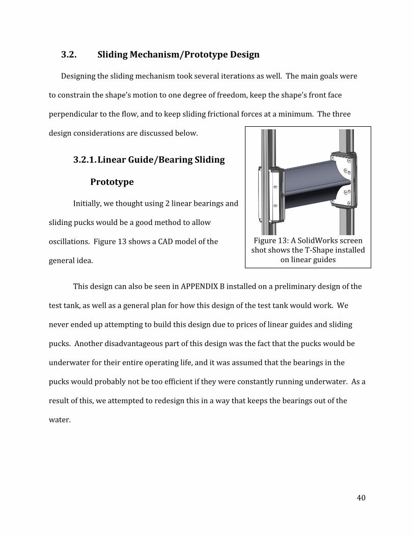
Figure 13: A SolidWorks screen
shot shows the T-Shape installed on linear guides
3.2. Sliding Mechanism/Prototype Design
Designing the sliding mechanism took several iterations as well. The main goals were
to constrain the shape’s motion to one degree of freedom, keep the shape’s front face
perpendicular to the flow, and to keep sliding frictional forces at a minimum. The three
design considerations are discussed below.
3.2.1. Linear Guide/Bearing Sliding
Prototype
Initially, we thought using 2 linear bearings and
sliding pucks would be a good method to allow
oscillations. Figure 13 shows a CAD model of the
general idea.
This design can also be seen in APPENDIX B installed on a preliminary design of the
test tank, as well as a general plan for how this design of the test tank would work. We
never ended up attempting to build this design due to prices of linear guides and sliding
pucks. Another disadvantageous part of this design was the fact that the pucks would be
underwater for their entire operating life, and it was assumed that the bearings in the
pucks would probably not be too efficient if they were constantly running underwater. As a
result of this, we attempted to redesign this in a way that keeps the bearings out of the
water.
41
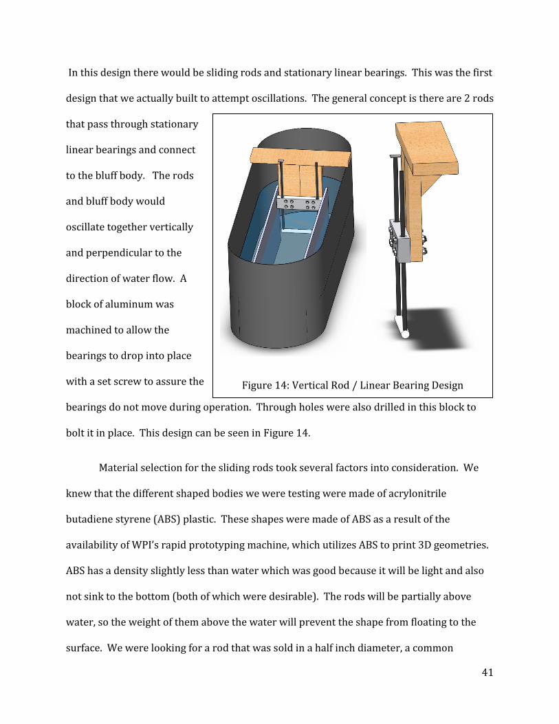
Figure 14: Vertical Rod / Linear Bearing Design
In this design there would be sliding rods and stationary linear bearings. This was the first
design that we actually built to attempt oscillations. The general concept is there are 2 rods
that pass through stationary
linear bearings and connect
to the bluff body. The rods
and bluff body would
oscillate together vertically
and perpendicular to the
direction of water flow. A
block of aluminum was
machined to allow the
bearings to drop into place
with a set screw to assure the
bearings do not move during operation. Through holes were also drilled in this block to
bolt it in place. This design can be seen in Figure 14.
Material selection for the sliding rods took several factors into consideration. We
knew that the different shaped bodies we were testing were made of acrylonitrile
butadiene styrene (ABS) plastic. These shapes were made of ABS as a result of the
availability of WPI’s rapid prototyping machine, which utilizes ABS to print 3D geometries.
ABS has a density slightly less than water which was good because it will be light and also
not sink to the bottom (both of which were desirable). The rods will be partially above
water, so the weight of them above the water will prevent the shape from floating to the
surface. We were looking for a rod that was sold in a half inch diameter, a common

42
diameter for bar stock, and the diameter of the purchased linear bearings. The problem we
encountered was that with lighter materials, the Young’s Modulus of the material also
tended to decrease. Since the approximate flow velocities were known, and the diameters
of the shapes were known, we were able to calculate the drag force that the object would
feel during the flow. The rods act as cantilever beams, fixed at one end (the bearings) and
subject to a load at the free end. The load at the free end is equivalent to the drag force,
which can be calculated using
. In this formula, the drag force is dependent
upon the mass density of water; u, the velocity of object relative to the fluid; , the drag
coefficient for the given shape (value taken from Fluent); and A, the cross-sectional area
(facing the fluid flow) of the shape.
With the load on the rods known and the diameter and Young’s moduli for several
materials known, we searched for a material that was light and strong enough to deflect
less than 0.05 inches at a moment arm distance of 12 inches from the bearings (the
maximum possible). An example of the calculations performed to find the deflections are
shown in APPENDIX C: MATHCAD CALCULATIONS FOR STRESS AND DEFLECTION OF
OSCILLATING RODS. Additionally, the stress in the beam was calculated to ensure it would
be well below the yield strength to avoid plastic deformation during normal operation.
APPENDIX E: A TABLE USED IN THE MATERIAL SELECTION PROCESS FOR THE
OSCILLATING RODS was used to help select a material by organizing materials based on
cost and material properties. The material selected was Noryl, which is a combination of
Polyphenylene Oxide (PPO) and Polystyrene (PS).

43
Figure 15: Horizontally Oscillating Design with Pump Configuration
Springs were used to support the weight of the oscillating components. The initial
displacement of these springs determined the equilibrium position of the test shape; and
this initial displacement was chosen so that at equilibrium the test shape would remain in
the center of the testing area. The position sensor would be located above the sliding
mechanism and would be pointed towards a plate that was secured to one of the rods (as
shown in Figure 14 above). After building this prototype and placing it in our test tank, the
team discovered that the friction forces from the rods sliding through the bearings were
too great. The lift forces generated from the vortices were not great enough to initiate
oscillations. We tried sanding the rods and using lubricants to minimize friction forces, but
oscillations could not be achieved, therefore a new design was necessary.
3.2.2. Horizontally Oscillating Slider Prototype
To eliminate gravity as a factor, we
decided to try using horizontal oscillations of
the shape. To do this we secured a standard
drawer slide to a piece of plywood. We then
secured one end of the shape to the sliding
component of the drawer slide. To do this we
drilled a hole in the end of the ABS plastic
shapes and used a self-tapping screw. This
design with the pump configuration is shown
in Figure 15.

44
This design proved to work very well. Steady, large oscillations were maintained at
even very slow water speeds. To measure the position of the shape, a rod was installed
vertically into the top of each shape, with a plate added to the top of it. This plate served as
a surface in which the position sensor could easily read its location. The position sensor
was suspended from a stand and positioned pointing at this plate. This configuration was
used to test all 3 shapes at 3 different flow speeds. This is explained further in the testing
methods section and can also be seen in APPENDIX D.
45
4. Methodology
The primary goal of this project was to develop a more efficient cross sectional
shape for generating vortices focusing on the lift forces created by the vortices. To do this
we also needed to create a water tank capable of variable flow speeds, continual tests, and
limited fluid disturbances from wakes, eddies, and inconsistent flow profiles. Additionally,
a test stand needed to be developed to allow for oscillations from Vortex Induced
Vibrations with as little friction as possible, maximizing the efficiency with hopes for
energy generation. Finally, it was important collect enough data to allow for further work
in the development of a more efficient collection method, harnessing the higher oscillatory
lift forces as a form of renewable energy. The following sections of this report will
thoroughly describe the steps taken to reach all of these goals.
4.1. ANSYS Fluent Testing Methods
In order to find which general shape would create the highest lift force, FEA tests were
first conducted for some basic shapes, which are described later in the methodology, using
Ansys 12 Fluent. Initially, trials were conducted by using a diameter of .0254 m
(approximately 1 in) and changing the velocity of the water to achieve the desired
Reynolds number. This method was chosen for the intent of simulating the small scale
physical testing. However, the program was unable to give accurate results due to the large
size of the mesh being used. Attempts to use a smaller size mesh required a much longer
amount of CPU time to test each shape, which was unacceptable given the time allowed for
the study’s completion. Therefore, using the test method described below, more accurate
results were able to be produced in a more efficient time period.
46
The FEA tests were conducted using a 2 dimensional geometry in the X and Y
directions of the coordinate system and assumed infinite length in the Z direction. The
boundaries of the flow field were 20 times the characteristic length (i.e. diameter) high by
30 times the characteristic length wide. This size test area allowed for minimal boundary
layer effects on the flow, which was intended to simulate an infinitely wide channel. The
shape was positioned at 10 times the characteristic length down from the top, and 10 times
the characteristic length to the right of the inlet. The tests were conducted using the
following Reynold’s numbers: 100, 150, 200, 500, 1000, 2000, 3000, 4000, and 5000. The
characteristic length of the shape was kept constant at one meter, and the density property
of fluid was varied to achieve the desired Reynold’s number. This approach was used
because it was most convenient parameter to change to obtain the specific Reynold’s
number desired, where as changing the velocity, for example, would have taken extra
calculations. The flow was set at transient flow with a constant dynamic viscosity of 1
N*s/m2 and a constant velocity of 1 m/s. Once the basic Shapes had been tested, the T-
shape was found to have the largest lift coefficient. variations of the T-shape were then
tested using the same methods as the basic shape test. The top three variations of the T-
shape, as well as the basic T-shape for comparison, were then tested at Reynold’s numbers
of 6000, 7000, and 8000 in order to determine how each shape would perform under faster
flow conditions. The last part of the FEA analysis included testing the shapes at the
estimated Reynolds number for the simulated flow of water at operating conditions. The
same test method as described above was used except for the following changes to the
properties: density was assumed to be 999 kg/m3, dynamic viscosity was assumed to be
1.12*10-3 N*s/m2, velocity was assumed to be 1.03 m/s (approximately 2 knots), and the

47
diameter was assumed to be .15 m (approximately 6 in). These parameters resulted in a
Reynolds number of approximately 140,000.
The basic shapes tested included a square, rectangle, triangle, and ellipse. These
shapes can be viewed in Figure (added when known). The varied T-shapes tested included
a cylindrical T, a triangular T, a parachute T, a Y T, and a concave T. These shapes can be
view in Figure (added when known).The triangle went through two rounds of testing: one
round with the point into the flow, and one with point away from the flow. The ellipse went
through two round of testing as well: one with the semi-major axis perpendicular with the
flow, and one with the semi-major axis perpendicular to the flow. The T-shape was tested
with the flat top into the flow. Similarly to the basic T-shape, the variations of T-shapes
were tested with the T part facing into the flow.
4.2. Test Tank Construction
The test tank was built based around a 6’ x 2’ x 2’ steel, oval water trough to ensure
the water holding capacity of the system. The system consisted of a test channel, a
diffuser, an oscillation testing stand, a converger, and 3 pumps. The construction, setup,
and operation of these subsystems can be found in the following section.
4.2.1. Test Channel

48
The test channel had a simple construction
with three 4 ft. boards of sealed particle board.
Two of these boards were 16” wide and were used
as the side boards. The bottom board was 11 ¾”
wide for the purposes of press fitting the diffuser
(see section below) into the channel. The side
boards were attached to the bottom board with 4
“L” brackets. After the basic channel was
constructed, weather stripping was added around
the exposed edges of the front and back while
caulking was used as a waterproofing method on the joints. Finally, wooden handles (2” x
2” x 12”) were attached across the top of the test channel for removing the channel from
the test tank. This allowed the tank to stay filled with water while the test channel could be
dried when not in use as seen in Figure 17.
4.2.2. Diffuser
The diffuser was built to create a more
uniform velocity profile concentrated around the
area where most of our testing occurred.
Eliminating turbulence upstream from the testing
area provided more repeatable results. We used
18’ of 1 ¼" diameter PVC pipe with a wall thickness
of 1/16” as well as 14’ of ¾" diameter PVC pipe
with a wall thickness of 1/16”. The PVC pipe was cut into 3” sections. These sections of
Figure 16: Channel for Test Tank
Figure 17: Test Channel for Test Tank
Figure 18: Diffuser for Test Tank
49
pipe were glued together using waterproof plumber’s glue in the orientation shown in
Figure 18.
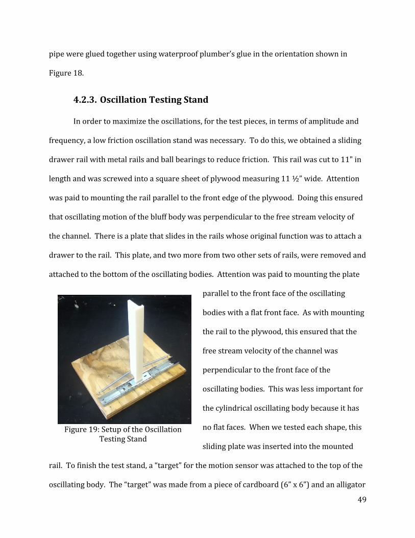
4.2.3. Oscillation Testing Stand
In order to maximize the oscillations, for the test pieces, in terms of amplitude and
frequency, a low friction oscillation stand was necessary. To do this, we obtained a sliding
drawer rail with metal rails and ball bearings to reduce friction. This rail was cut to 11" in
length and was screwed into a square sheet of plywood measuring 11 ½” wide. Attention
was paid to mounting the rail parallel to the front edge of the plywood. Doing this ensured
that oscillating motion of the bluff body was perpendicular to the free stream velocity of
the channel. There is a plate that slides in the rails whose original function was to attach a
drawer to the rail. This plate, and two more from two other sets of rails, were removed and
attached to the bottom of the oscillating bodies. Attention was paid to mounting the plate
parallel to the front face of the oscillating
bodies with a flat front face. As with mounting
the rail to the plywood, this ensured that the
free stream velocity of the channel was
perpendicular to the front face of the
oscillating bodies. This was less important for
the cylindrical oscillating body because it has
no flat faces. When we tested each shape, this
sliding plate was inserted into the mounted
rail. To finish the test stand, a “target” for the motion sensor was attached to the top of the
oscillating body. The “target” was made from a piece of cardboard (6” x 6”) and an alligator
Figure 19: Setup of the Oscillation
Testing Stand

50
clip on a wire that fits into the small hole drilled at the top oscillating body. A picture of the
Oscillating Test Stand can be seen in Figure 19.
4.2.4. Converger
The converger was used to redirect the flow of the water down the test channel. It
was constructed out of thin, pliable sheet metal with each sheet measuring 12” high and
24” long. The converger can be seen in Figure 21 which illustrates the full tank setup. Each
half of the converger was initially molded to the ridges in the water trough with a rubber
mallet. Caulking was used to seal any other leaks. The converger was connected together
after bending the sheet metal in a semicircular fashion, aiming the water down the test
channel.
4.2.5. Submersible Pumps
To allow for three different flow rates, different combinations or configurations of
three submersible pumps were used. The lowest flow rate tested was achieved by turning
on 1 central 1/3 horsepower sump
pump. This was called “flow rate 1”.
The 2nd flow rate was achieved by
turning on 2 ¼ horsepower sump
pumps, utilizing ½ horsepower of sump
pumps total (“flow rate 2”). The fastest
flow rate tested used all 3 sump pumps
(the 2-1/4 horsepower and the 1/3 horsepower pumps) utilizing 5/6 horsepower of sump
pumps total (“flow rate 3”). The position of these pumps can be seen in Figure 20.
Figure 20: Pump Setup and Configurations

51
4.2.6. Test Tank Setup
Prior to testing, the team secured the test channel in the proper location in the tank.
The channel was secured parallel with the sides of the tank and has 5” of clearance on
either side for the recirculation channels. The channel should also be centered lengthwise
in the tank providing space
for the pumps in the rear
and the converger in the
front. The channel was
secured with 5 lb. weights
on each side of each
support on the protruding
screws. Completing the
setup of the test tank
required assuring that the
pumps and converger are in their proper location. After this was completed, the test tank
was filled with water up to the top of the converger, creating a depth of 12”. Figure 21
illustrates the proper setup of the set tank.
Test Equipment Utilized
To record the data necessary, several types of testing equipment were utilized. A
Vernier LabPro interface (order number: LABPRO) connected the sensors to a computer.
The two sensors used plugged into the interface, and the interface was connected to a
laptop computer via USB. The first sensor used, a Vernier Flow Rate Sensor (order
number: FLO-BTA), determined the flow velocities at certain points in the fluid flow. The
Figure 21: Secured Setup of Tank Elements

52
Figure 22: From Left to Right: Vernier LabPro, Flow Rate Sensor, and Motion Detector.
second sensor was to determine the position of our cylinders with respect to time. To
measure this, a Vernier Motion Detector (order number: MB-BTD) was utilized. Figure 22
Error! Reference source not found.shows company photos of the test equipment:
The Vernier LabPro interface was used in conjunction with a laptop through a USB
port and the LoggerPro software from Vernier. It has the ability to take 50,000 readings
per second and can hold up to 12,000 data points with a 12-bit A/D Conversion.
The Flow Rate Sensor measures the velocity of a fluid by using an impeller. As the
fluid passes over the impeller, the impeller rotates, subsequently rotating a bar magnet
attached to the impeller’s shaft. A read switch monitors the change in the magnetic field as
the magnet rotates and converts this signal into a voltage. The output voltage is therefore
proportional to the velocity of the fluid and is calibrated with the LabPro interface. When
plugged into the Channel 1 input, the Flow Rate Sensor has a resolution of 0.0012 m/s and
an accuracy of ±1% of a full scale reading with a velocity range of 0 to 4.0 m/s.

53
The Motion Detector 2 emits a short ultrasonic pulse from the transducer and
registers the time it takes for the pulse to return. By comparing this to the speed of sound
in air, the Motion Detector 2 can output the distance to the object causing the echo with a
resolution of 1mm and an accuracy of 2 mm. It has a range of 0.15 m to 6 m and an optimal
collection rate of 20 samples per second however, it is important that objects within a 15°
to 20° cone are removed from the test area to make sure that the proper object is being
targeted.
4.3. Determining the Velocity Profile at the Test Area
The velocity profile was determined at the test area for the 3 different fluid flow
rates. The three different flow rates were created by different combinations of sump
pumps. The lowest flow rate (velocity 1) tested was achieved by turning on 1 central 1/3
horsepower sump pump. This will be called flow velocity 1.The 2nd flow rate (velocity 2)
was achieved by turning on two ¼ horsepower sump pumps, utilizing ½ horsepower of
sump pumps total. The fastest flow rate (velocity 3) tested used all 3 sump pumps (the 2-
1/4 horsepower and the 1/3 horsepower pumps) utilizing 5/6 horsepower of sump pumps
total. Figure 23 shows the position of these pumps and how their PVC piping was set up.
Figure 23: Pump Arrangement with Pumps Labeled (CAD Model and Prototype)

54
The velocities at 11 chosen positions were measured for each of the pump
configurations. To gain the velocity data for each of the 11 position, 500 data points of the
velocity were taken
over a 20 second time
interval. Figure
24Error! Reference
source not found.
shows a layout of the
dimensions of these 11
positions with the
nomenclature used for
each position.
The velocities were measured at
each of the 11 locations for each of the 3
flow rates. The velocities were
measured 3 times for each location at
each flow rate. These three trials were
averaged for a given point at a given flow
rate to determine an accepted value.
Each trial took the average flow rate over a 20 second interval. Figure 25 shows this test
setup.
Figure 24: Velocity Profile Locations and Nomenclature
Figure 25: Setup for Velocity Profile Testing
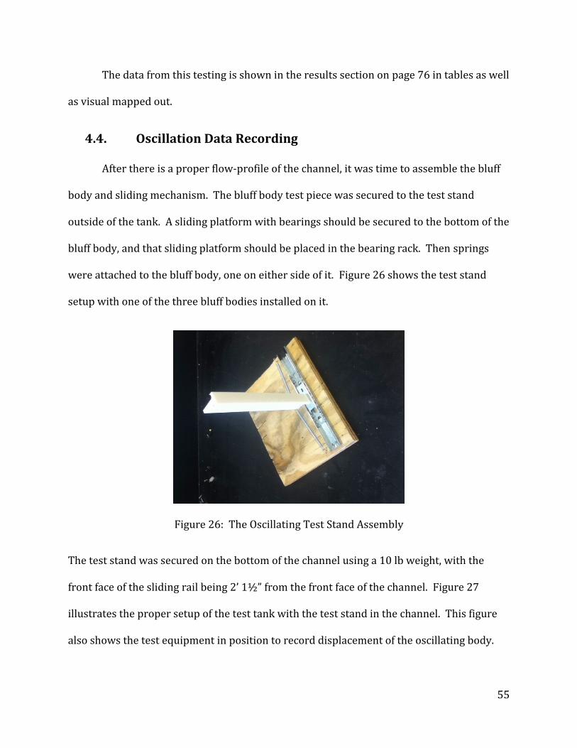
55
The data from this testing is shown in the results section on page 76 in tables as well
as visual mapped out.
4.4. Oscillation Data Recording
After there is a proper flow-profile of the channel, it was time to assemble the bluff
body and sliding mechanism. The bluff body test piece was secured to the test stand
outside of the tank. A sliding platform with bearings should be secured to the bottom of the
bluff body, and that sliding platform should be placed in the bearing rack. Then springs
were attached to the bluff body, one on either side of it. Figure 26 shows the test stand
setup with one of the three bluff bodies installed on it.
Figure 26: The Oscillating Test Stand Assembly
The test stand was secured on the bottom of the channel using a 10 lb weight, with the
front face of the sliding rail being 2’ 1½” from the front face of the channel. Figure 27
illustrates the proper setup of the test tank with the test stand in the channel. This figure
also shows the test equipment in position to record displacement of the oscillating body.
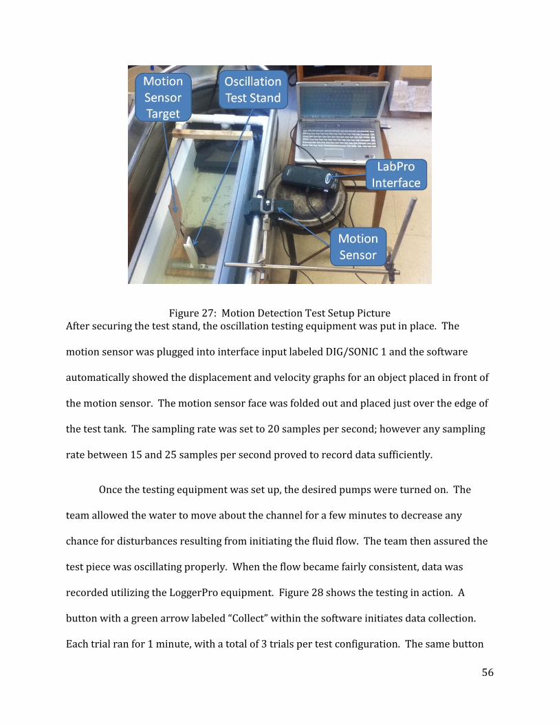
56
Figure 27: Motion Detection Test Setup Picture After securing the test stand, the oscillation testing equipment was put in place. The
motion sensor was plugged into interface input labeled DIG/SONIC 1 and the software
automatically showed the displacement and velocity graphs for an object placed in front of
the motion sensor. The motion sensor face was folded out and placed just over the edge of
the test tank. The sampling rate was set to 20 samples per second; however any sampling
rate between 15 and 25 samples per second proved to record data sufficiently.
Once the testing equipment was set up, the desired pumps were turned on. The
team allowed the water to move about the channel for a few minutes to decrease any
chance for disturbances resulting from initiating the fluid flow. The team then assured the
test piece was oscillating properly. When the flow became fairly consistent, data was
recorded utilizing the LoggerPro equipment. Figure 28 shows the testing in action. A
button with a green arrow labeled “Collect” within the software initiates data collection.
Each trial ran for 1 minute, with a total of 3 trials per test configuration. The same button
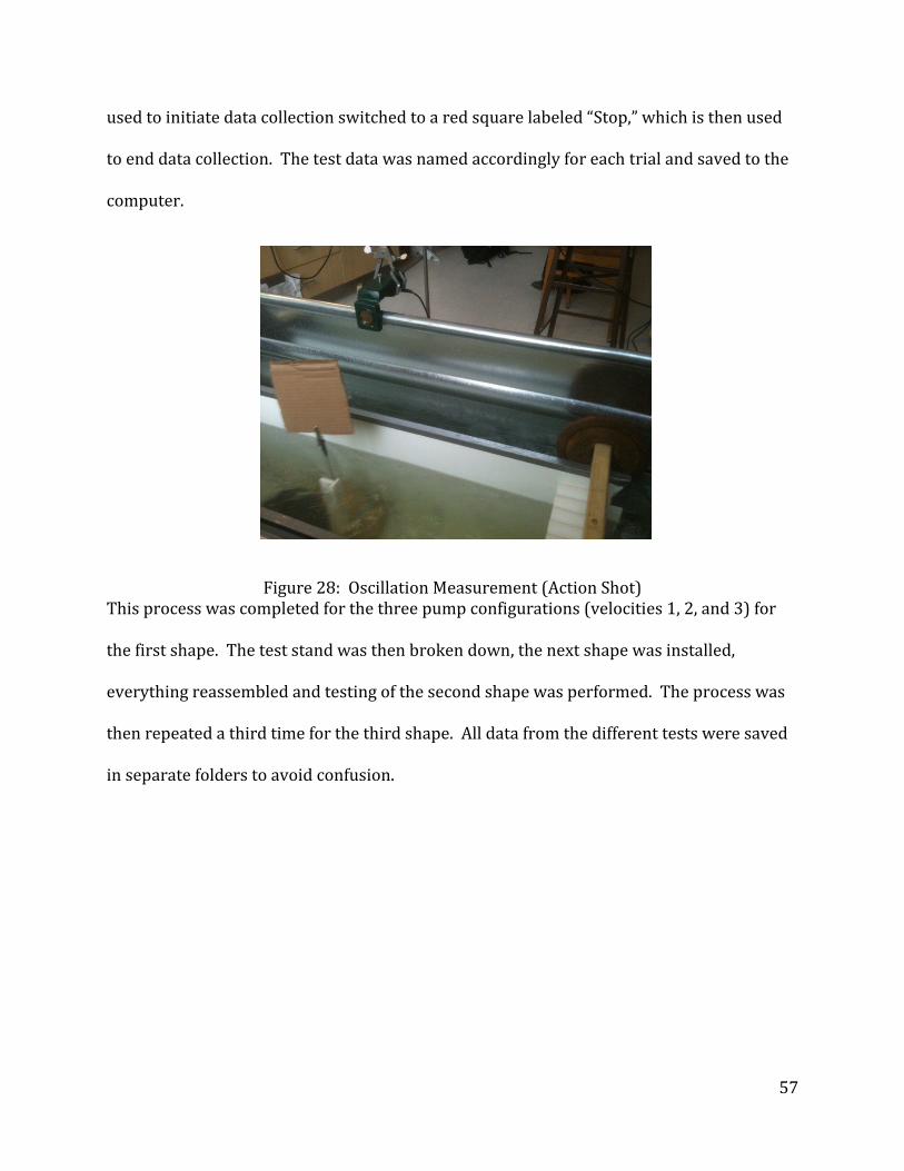
57
used to initiate data collection switched to a red square labeled “Stop,” which is then used
to end data collection. The test data was named accordingly for each trial and saved to the
computer.
Figure 28: Oscillation Measurement (Action Shot) This process was completed for the three pump configurations (velocities 1, 2, and 3) for
the first shape. The test stand was then broken down, the next shape was installed,
everything reassembled and testing of the second shape was performed. The process was
then repeated a third time for the third shape. All data from the different tests were saved
in separate folders to avoid confusion.

58
5. Results and Analysis
5.1 Fluent FEA Trials for Basic Shapes
In order to find which general shape would create the highest lift force, FEA tests
were first conducted for some basic shapes using Ansys 12 Fluent tests. As stated
previously, these tests were done using a 2 dimensional geometry in the X and Y directions
of the coordinate system and assumed infinite length in the Z direction. The boundaries of
the flow field were 20 times the characteristic length high by 30 times the characteristic
length wide. The shape was positioned at 10 times the characteristic length down from the
top, and 10 times the characteristic length to the right of the inlet. The tests were
conducted using the following Reynold’s numbers: 100, 150, 200, 500, 1000, 2000, 3000,
4000, and 5000. The characteristic length of the shape (i.e. diameter) was kept constant at
one meter, and the density property of fluid was varied to achieve the desired Reynold’s
number. The flow was set at transient flow with a constant dynamic viscosity of 1 N*s/m2
and a constant velocity of 1 m/s. The basic shapes tested can be viewed in Figure 29, and
include a square, rectangle, triangle, and ellipse. The triangle went through two rounds of
testing: one round with the point into the flow, and one with point away from the flow. The
ellipse went through two round of testing as well: one with the semi-major axis
perpendicular with the flow, and one with the semi-major axis perpendicular to the flow.
The T-shape was tested with the flat top into the flow.

59
Figure 29: Overview of Basic Shapes
The first shape tested was the triangle. The first triangle test was conducted with
the point of the triangle into the flow. The lift coefficient at low Reynold’s numbers was
0.0001, and was 0.01 at higher Reynold’s numbers. The second triangle test was conducted
with the point facing away from the flow. The resulting lift coefficient was much better
than the previous way the triangle was tested. At low Reynold’s numbers the lift coefficient
was around 0.08, while at higher Reynold’s numbers the lift coefficient was about 1.4. This
test clearly shows the triangle has higher performance with tip facing away from the flow,
instead of into the flow as previously suggested by background research. The lift coefficient
graph as well as the vorticity and pressure charts for the triangle can be viewed in Figure
30.
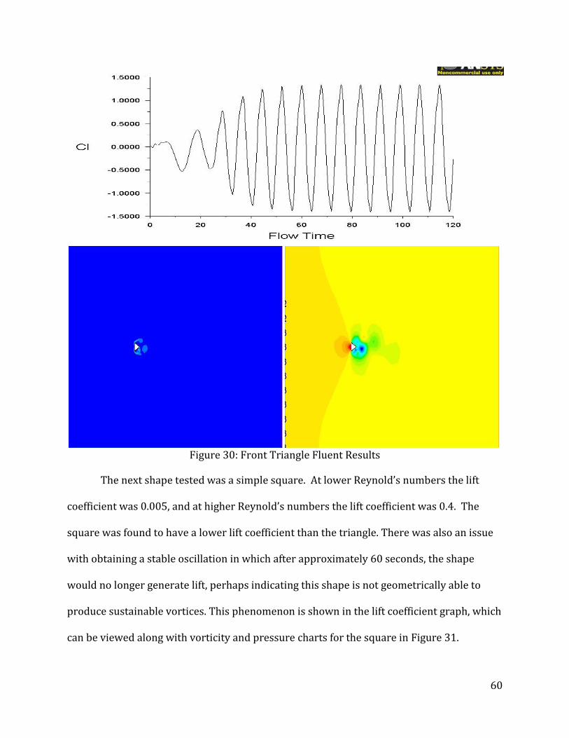
60
Figure 30: Front Triangle Fluent Results
The next shape tested was a simple square. At lower Reynold’s numbers the lift
coefficient was 0.005, and at higher Reynold’s numbers the lift coefficient was 0.4. The
square was found to have a lower lift coefficient than the triangle. There was also an issue
with obtaining a stable oscillation in which after approximately 60 seconds, the shape
would no longer generate lift, perhaps indicating this shape is not geometrically able to
produce sustainable vortices. This phenomenon is shown in the lift coefficient graph, which
can be viewed along with vorticity and pressure charts for the square in Figure 31.

61
Figure 31: Square Fluent Results
The next shape tested was the ellipse. The first test included an ellipse with length
to width ratio (L/W) of one quarter. At lower Reynolds’s numbers, the lift coefficient was
found to be 0.02, and at higher Reynolds’s numbers was found to be 0.1. The ellipse also
experienced the same phenomenon as the square, in which it would no longer produce lift
forces after 60 seconds. The second test included an ellipse with an L/W of two. At lower
Reynolds’s numbers the lift coefficient was found to be 0.035, and at higher Reynolds’s
numbers, the shape failed to produce oscillating lift coefficients. Due to the inability of the
ellipse to generate oscillating lift coefficients, this shape is not recommended for the use of

62
generating vortices. The lift coefficient graph as well as the vorticity and pressure charts
for the ellipse can be viewed in Figures 32 and 33.
Figure 32: Ellipse L/W = 0.25 Fluent Results
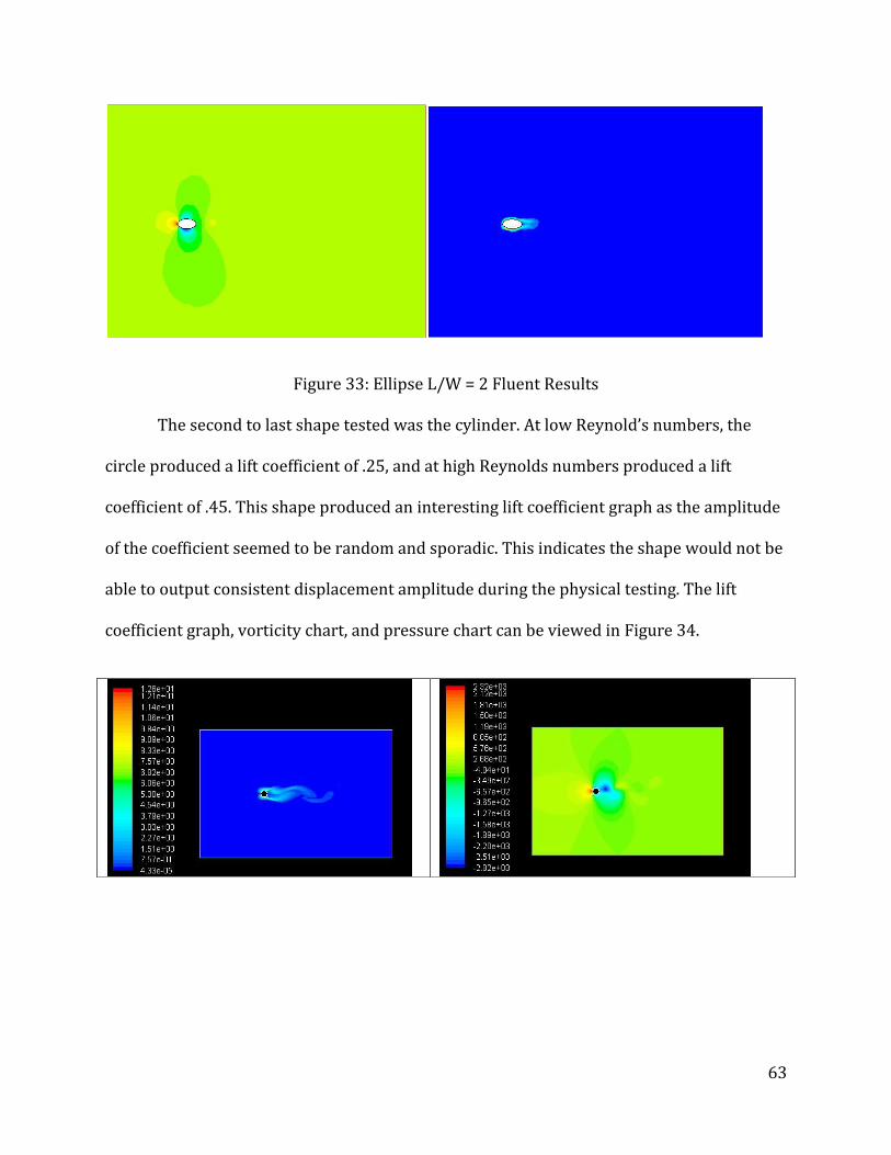
63
Figure 33: Ellipse L/W = 2 Fluent Results
The second to last shape tested was the cylinder. At low Reynold’s numbers, the
circle produced a lift coefficient of .25, and at high Reynolds numbers produced a lift
coefficient of .45. This shape produced an interesting lift coefficient graph as the amplitude
of the coefficient seemed to be random and sporadic. This indicates the shape would not be
able to output consistent displacement amplitude during the physical testing. The lift
coefficient graph, vorticity chart, and pressure chart can be viewed in Figure 34.

64
The final shape tested was the T-shape. This shape produced a lift coefficient of .17
at low Reynold’s numbers and a lift coefficient of 1.8 at high Reynold’s numbers. This shape
produced the largest lift coefficients out of all the other basic shapes, and was selected to
determine which shape variation would produce the largest lift coefficient. One possible
theory about why the T-shape produced the largest amplitudes was that it had a flat face
into the flow, and the horizontal piece of the T (as viewed in Figure 37) acted as a splitter
plate allowing the force of the pressure difference to act on the shape for a longer period of
time. The lift coefficient graph as well as the vorticity and pressure charts for the T-shape
can be viewed in Figure 37.
Figure 34: Circle Fluent Results
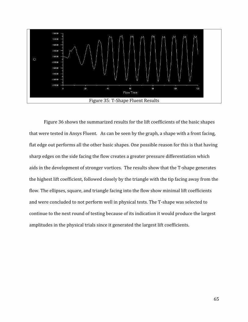
65
Figure 36 shows the summarized results for the lift coefficients of the basic shapes
that were tested in Ansys Fluent. As can be seen by the graph, a shape with a front facing,
flat edge out performs all the other basic shapes. One possible reason for this is that having
sharp edges on the side facing the flow creates a greater pressure differentiation which
aids in the development of stronger vortices. The results show that the T-shape generates
the highest lift coefficient, followed closely by the triangle with the tip facing away from the
flow. The ellipses, square, and triangle facing into the flow show minimal lift coefficients
and were concluded to not perform well in physical tests. The T-shape was selected to
continue to the next round of testing because of its indication it would produce the largest
amplitudes in the physical trials since it generated the largest lift coefficients.
Figure 35: T-Shape Fluent Results

66
Figure 36: Summarized Results of Basic Shapes from Fluent Testing
5.2 T-Shape Trials
After concluding the T-shape cylinder would produce the most lift out of the
common shapes, variations of the T-shape were tested in order to optimize the cross
sectional shape. These shapes include a circular T-shape, a triangular T-shape, a Y T-shape,
a parachute T-shape, a double-Y T-shape, and concave T-shape. These shapes can be
observed in Figure 37. As with the basic T-shape, all varied T-shapes were orientated with
the T part facing into the flow. A low Reynold’s number of 150 was compared with a high
Reynolds number of 5000.
00.10.20.30.40.50.60.70.80.9
11.11.21.31.41.51.61.71.81.9
0 1000 2000 3000 4000 5000 6000
Lift
Co
effi
cie
nt
Reynold's Number
Circle
T-Shape
Square
Front Triangle
Triangle
Ellipse L/W 0.25
Ellipse L/W =2
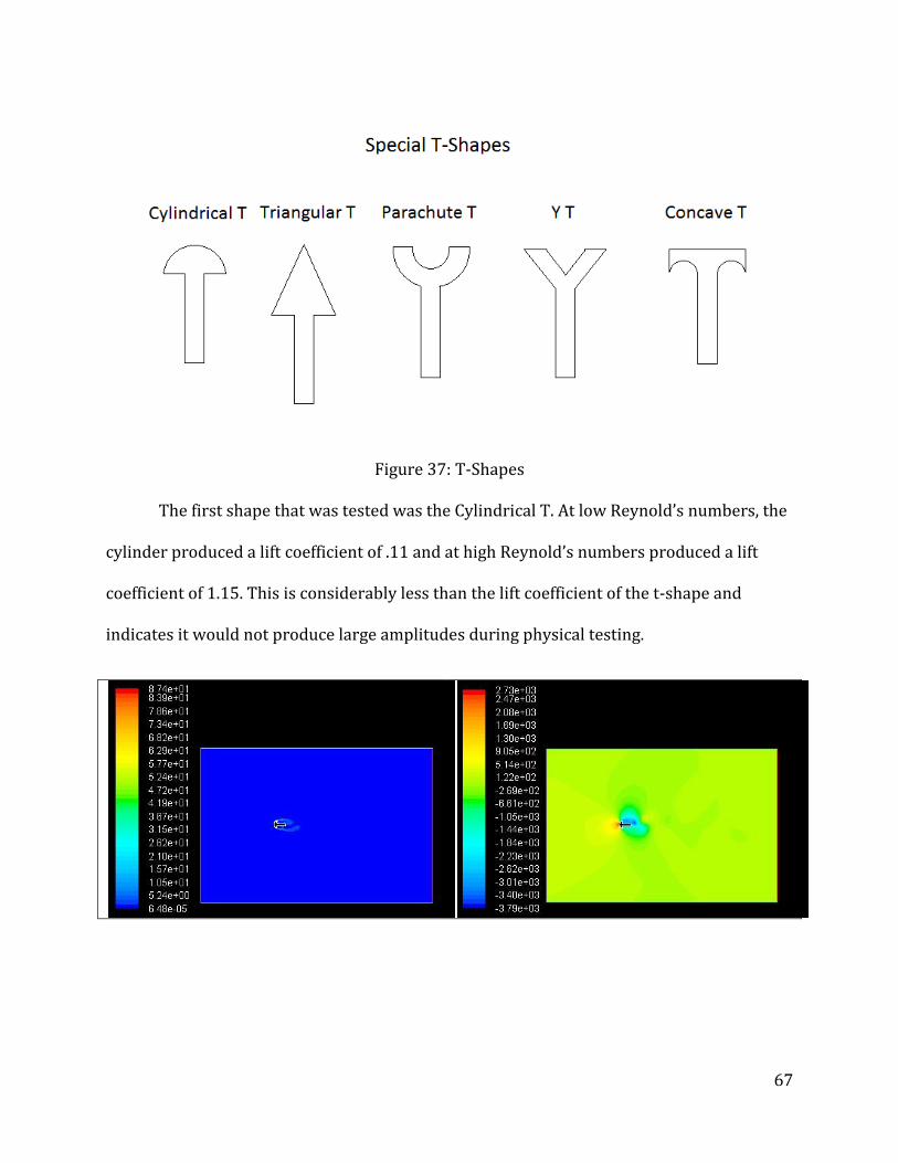
67
Figure 37: T-Shapes
The first shape that was tested was the Cylindrical T. At low Reynold’s numbers, the
cylinder produced a lift coefficient of .11 and at high Reynold’s numbers produced a lift
coefficient of 1.15. This is considerably less than the lift coefficient of the t-shape and
indicates it would not produce large amplitudes during physical testing.

68
Figure 38: Cylindrical T-Shape Fluent Results
The Triangle-T was tested next. It produced a lift coefficient of .01 at low Reynold’s
numbers and a lift coefficient of .85 at high Reynold’s numbers. Again, this lift coefficient
was much lower than the original T-shape.
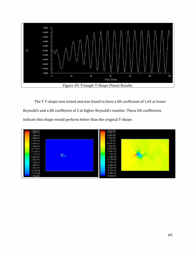
69
Figure 39: Triangle T-Shape Fluent Results
The Y T-shape was tested and was found to have a lift coefficient of 1.65 at lower
Reynold’s and a lift coefficient of 2 at higher Reynold's number. These lift coefficients
indicate this shape would perform better than the original T-shape.
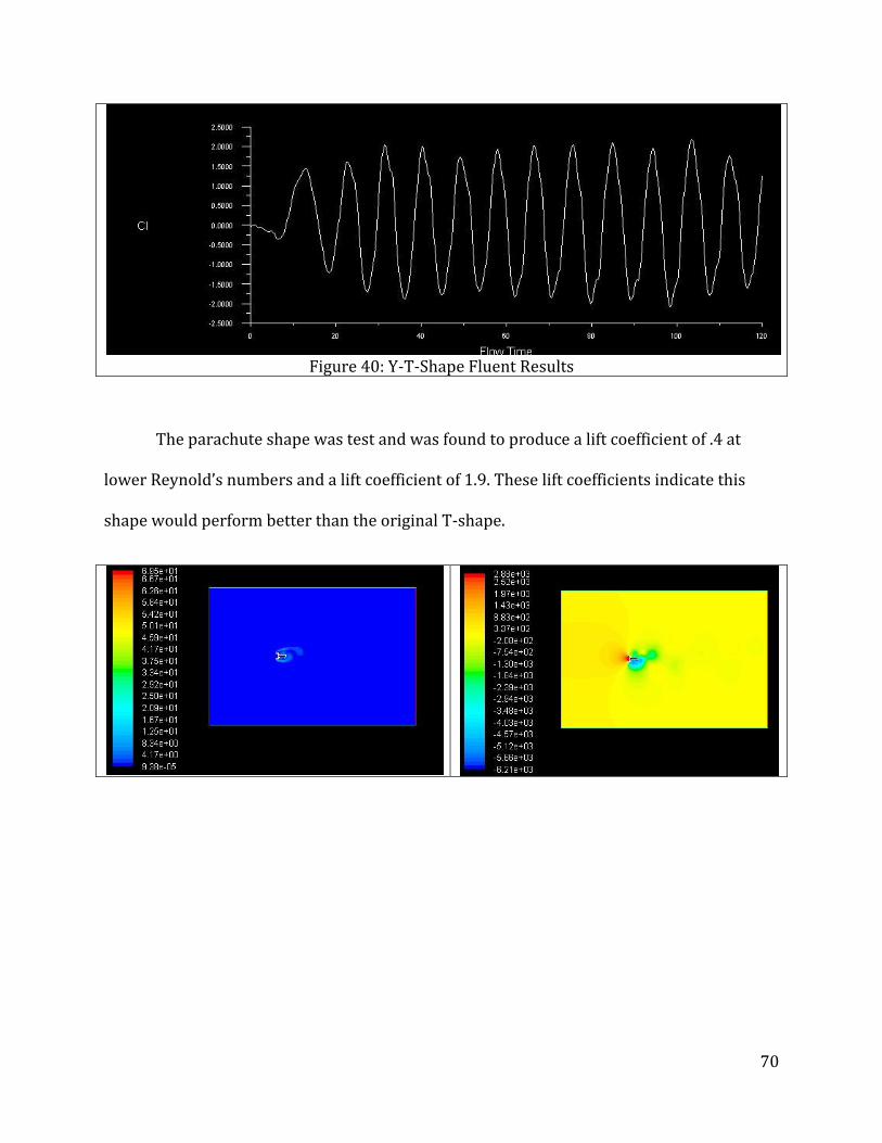
70
Figure 40: Y-T-Shape Fluent Results
The parachute shape was test and was found to produce a lift coefficient of .4 at
lower Reynold’s numbers and a lift coefficient of 1.9. These lift coefficients indicate this
shape would perform better than the original T-shape.

71
Figure 41: Parachute T-Shape Fluent Results
The last shape to be tested was the Concave-T shape which produced a lift
coefficient of .01 at low Reynold’s numbers and a lift coefficient of 2.2 at high Reynold’s
numbers. These lift coefficients suggest that this shape will perform better than the original
T-shape.

72
Figure 42: Concave T-Shape Fluent Results
Figure 42 shows a summary of the T-Shapes performance over a range of Reynolds
numbers. From this graph it is obvious that the Concave-T shape had the highest
performance in terms of the lift coefficient and the cylinder had the lowest performance.
Other shapes that performed well were the Parachute-T shape, the Y-T shape and regular
T-shape.
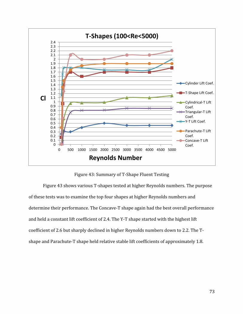
73
Figure 43: Summary of T-Shape Fluent Testing
Figure 43 shows various T-shapes tested at higher Reynolds numbers. The purpose
of these tests was to examine the top four shapes at higher Reynolds numbers and
determine their performance. The Concave-T shape again had the best overall performance
and held a constant lift coefficient of 2.4. The Y-T shape started with the highest lift
coefficient of 2.6 but sharply declined in higher Reynolds numbers down to 2.2. The T-
shape and Parachute-T shape held relative stable lift coefficients of approximately 1.8.
00.10.20.30.40.50.60.70.80.9
11.11.21.31.41.51.61.71.81.9
22.12.22.32.4
0 500 1000 1500 2000 2500 3000 3500 4000 4500 5000
Cl
Reynolds Number
T-Shapes (100<Re<5000)
Cylinder Lift Coef.
T-Shape Lift Coef.
Cylindrical-T LiftCoef.Triangular-T LiftCoef.Y-T Lift Coef.
Parachute-T LiftCoef.Concave-T LiftCoef.
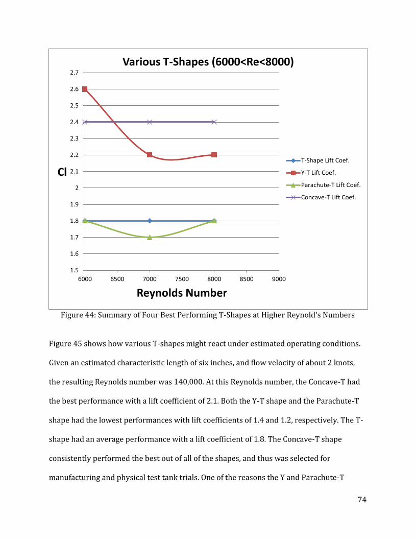
74
Figure 44: Summary of Four Best Performing T-Shapes at Higher Reynold's Numbers
Figure 45 shows how various T-shapes might react under estimated operating conditions.
Given an estimated characteristic length of six inches, and flow velocity of about 2 knots,
the resulting Reynolds number was 140,000. At this Reynolds number, the Concave-T had
the best performance with a lift coefficient of 2.1. Both the Y-T shape and the Parachute-T
shape had the lowest performances with lift coefficients of 1.4 and 1.2, respectively. The T-
shape had an average performance with a lift coefficient of 1.8. The Concave-T shape
consistently performed the best out of all of the shapes, and thus was selected for
manufacturing and physical test tank trials. One of the reasons the Y and Parachute-T
1.5
1.6
1.7
1.8
1.9
2
2.1
2.2
2.3
2.4
2.5
2.6
2.7
6000 6500 7000 7500 8000 8500 9000
Cl
Reynolds Number
Various T-Shapes (6000<Re<8000)
T-Shape Lift Coef.
Y-T Lift Coef.
Parachute-T Lift Coef.
Concave-T Lift Coef.
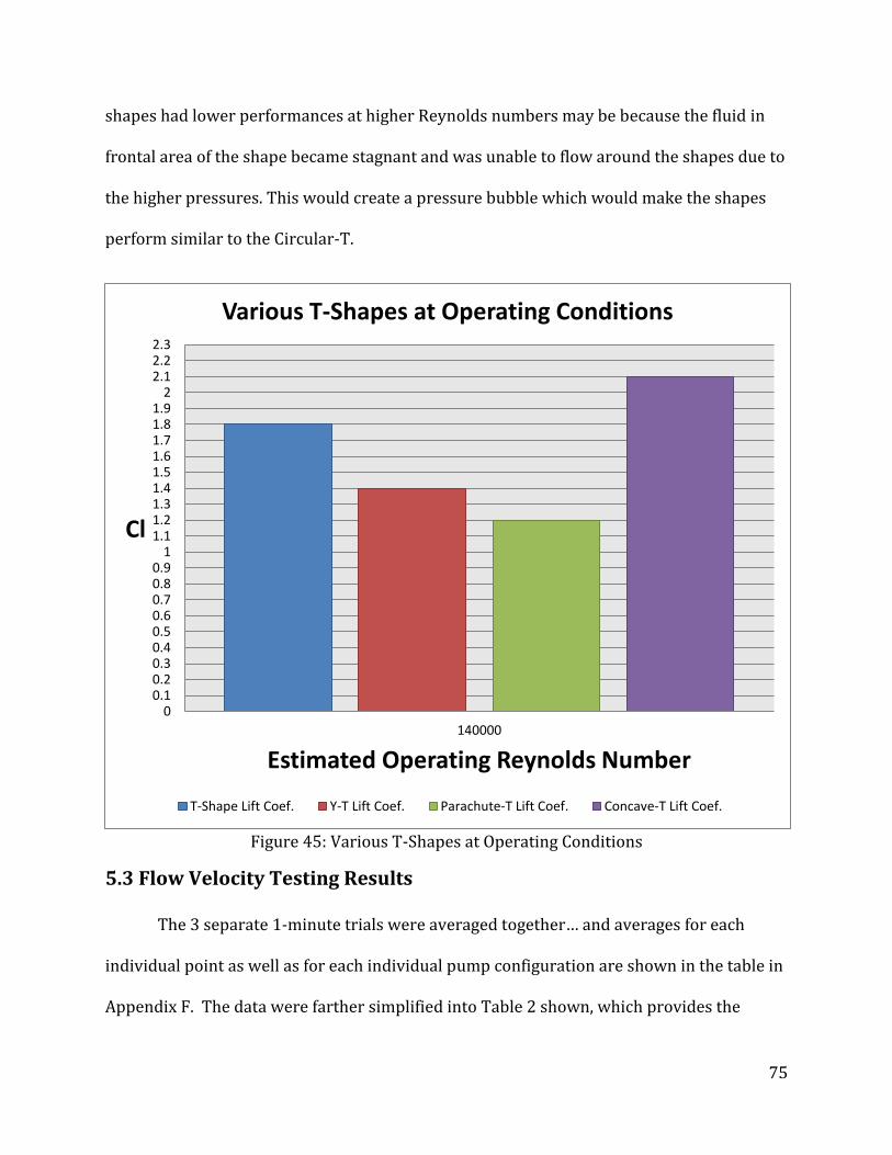
75
shapes had lower performances at higher Reynolds numbers may be because the fluid in
frontal area of the shape became stagnant and was unable to flow around the shapes due to
the higher pressures. This would create a pressure bubble which would make the shapes
perform similar to the Circular-T.
Figure 45: Various T-Shapes at Operating Conditions
5.3 Flow Velocity Testing Results
The 3 separate 1-minute trials were averaged together… and averages for each
individual point as well as for each individual pump configuration are shown in the table in
Appendix F. The data were farther simplified into Table 2 shown, which provides the
00.10.20.30.40.50.60.70.80.9
11.11.21.31.41.51.61.71.81.9
22.12.22.3
140000
Cl
Estimated Operating Reynolds Number
Various T-Shapes at Operating Conditions
T-Shape Lift Coef. Y-T Lift Coef. Parachute-T Lift Coef. Concave-T Lift Coef.
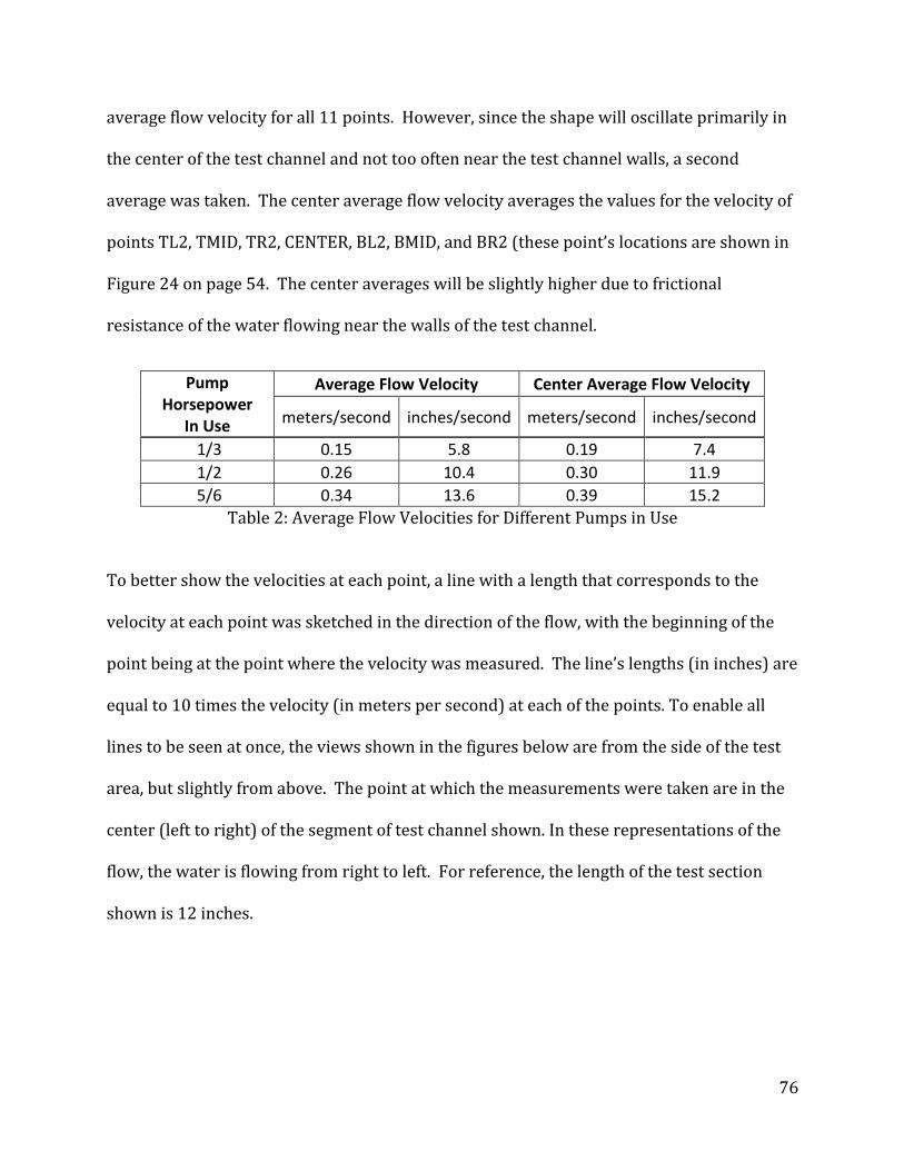
76
average flow velocity for all 11 points. However, since the shape will oscillate primarily in
the center of the test channel and not too often near the test channel walls, a second
average was taken. The center average flow velocity averages the values for the velocity of
points TL2, TMID, TR2, CENTER, BL2, BMID, and BR2 (these point’s locations are shown in
Figure 24 on page 54. The center averages will be slightly higher due to frictional
resistance of the water flowing near the walls of the test channel.
Pump Horsepower
In Use
Average Flow Velocity Center Average Flow Velocity
meters/second inches/second meters/second inches/second
1/3 0.15 5.8 0.19 7.4
1/2 0.26 10.4 0.30 11.9
5/6 0.34 13.6 0.39 15.2
Table 2: Average Flow Velocities for Different Pumps in Use
To better show the velocities at each point, a line with a length that corresponds to the
velocity at each point was sketched in the direction of the flow, with the beginning of the
point being at the point where the velocity was measured. The line’s lengths (in inches) are
equal to 10 times the velocity (in meters per second) at each of the points. To enable all
lines to be seen at once, the views shown in the figures below are from the side of the test
area, but slightly from above. The point at which the measurements were taken are in the
center (left to right) of the segment of test channel shown. In these representations of the
flow, the water is flowing from right to left. For reference, the length of the test section
shown is 12 inches.
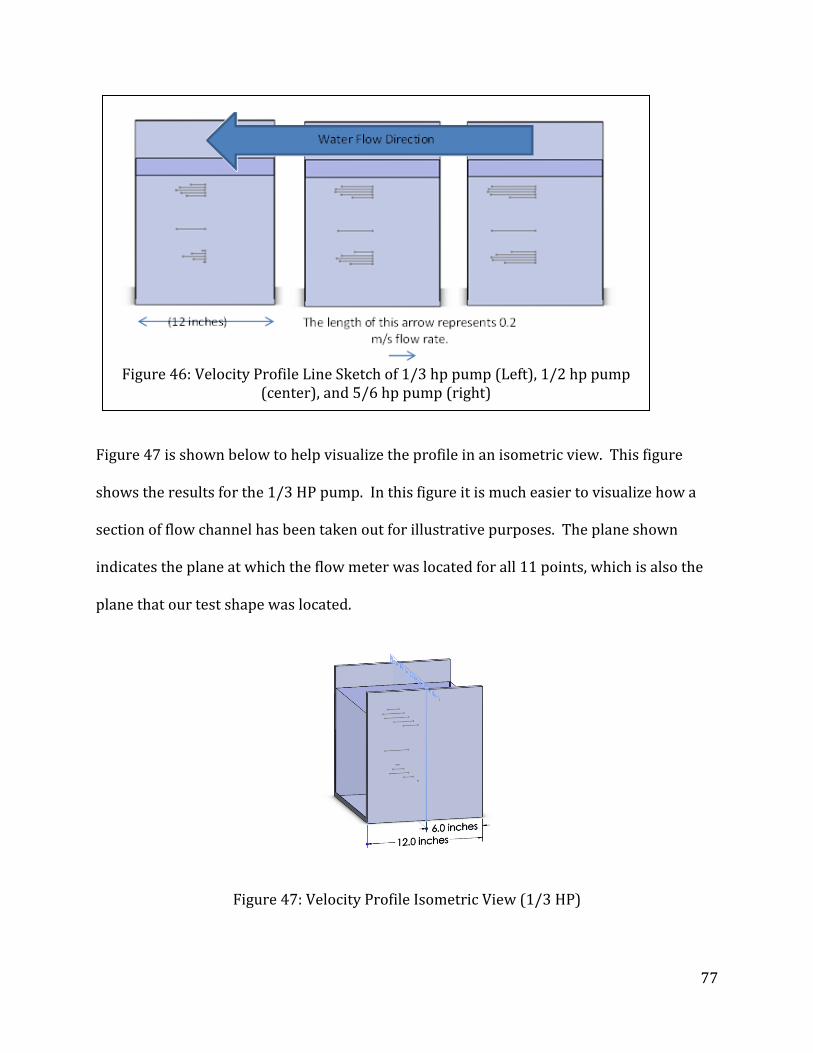
77
Figure 47 is shown below to help visualize the profile in an isometric view. This figure
shows the results for the 1/3 HP pump. In this figure it is much easier to visualize how a
section of flow channel has been taken out for illustrative purposes. The plane shown
indicates the plane at which the flow meter was located for all 11 points, which is also the
plane that our test shape was located.
Figure 47: Velocity Profile Isometric View (1/3 HP)
Figure 46: Velocity Profile Line Sketch of 1/3 hp pump (Left), 1/2 hp pump
(center), and 5/6 hp pump (right)

78
5.4 Physical Testing Results
After the testing of the shapes was finished, the results could then be determined
and conclusions could be determined. From the Logger Pro data we were able to record
and analyze the displacement of the shape. The curve produced was a sine curve, meaning
that the shape would move to one side and then back to the other side, with the zero point
being right in the middle of the channel. From interpretation of the data, we were able to
calculate an average displacement and plot that value versus the power of the pump.
Figure 48: Amplitude Results from Physical Testing
There were three tests conducted at each speed, and the graph above shows the
average displacement from each of the three test runs. As anticipated from the Fluent
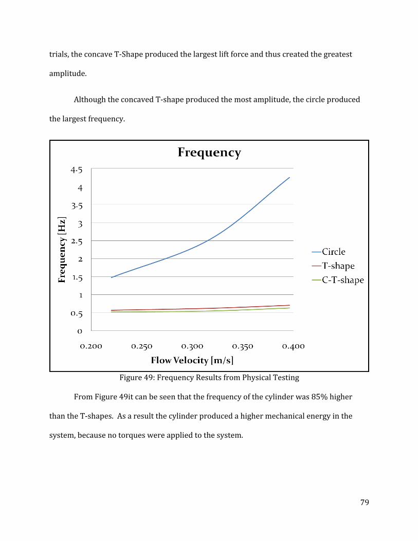
79
trials, the concave T-Shape produced the largest lift force and thus created the greatest
amplitude.
Although the concaved T-shape produced the most amplitude, the circle produced
the largest frequency.
Figure 49: Frequency Results from Physical Testing
From Figure 49it can be seen that the frequency of the cylinder was 85% higher
than the T-shapes. As a result the cylinder produced a higher mechanical energy in the
system, because no torques were applied to the system.
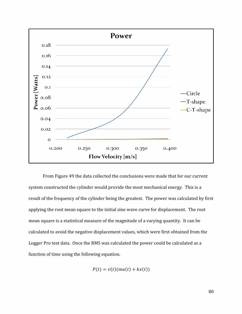
80
From Figure 49 the data collected the conclusions were made that for our current
system constructed the cylinder would provide the most mechanical energy. This is a
result of the frequency of the cylinder being the greatest. The power was calculated by first
applying the root mean square to the initial sine wave curve for displacement. The root
mean square is a statistical measure of the magnitude of a varying quantity. It can be
calculated to avoid the negative displacement values, which were first obtained from the
Logger Pro test data. Once the RMS was calculated the power could be calculated as a
function of time using the following equation.
81
In the above calculation v(t) represents the velocity at a certain time, m is the mass
of the object, and a(t) represents the acceleration of the shape. This first half of the
equation takes into account the moving shape and the second half accounts for the springs.
Where the k term is the spring constant determined from tests conducted earlier
specifically designed to find the value for the springs. And the x(t) term is the displacement
at a certain time.
The next set of data analyzed was the RMS force value, which was calculated by,
Where just as in the power equation the m and a(t) terms represent the force of the shape
and the k and x(t) terms represent the force of the springs.
82
6. Conclusions and Recommendations
The optimal cross sectional shape for generating renewable energy from vortex
induced vibrations is highly dependent upon the type of generator to be used. Different
types of generators are complimented by different design components in an oscillating
body when used in VIV energy generation. The larger forces produced by the “T” shapes
would favor a generator which produces energy by applying torque to the system. A
hydraulic generator could be considered with using “T” shapes as the oscillating body
because they operate at high torques and low velocities. The cylinder produced much
lower amplitudes and forces; however it generated much higher frequencies, favoring a
low torque generator, or an electromagnetic generator which is more dependent upon the
velocity and frequency of oscillations. Further work on this project will require a specific
generator to be selected or designed prior to optimizing the cross sectional shape of the
oscillating body.
6.1. Conclusions from Computer Simulations
Lift coefficients were compared when optimizing cross sectional shapes while
running FEA computer simulations. The team found that sharper trailing edges lead to
greater instances of vorticity while shapes with free stream geometries did not produce
vortices with the same magnitude. We feel that this is because the sharper trailing edges
left areas of low pressure, ideal to creating vortices. For example, a very evident
comparison was simply reversing the orientation of a triangle. When a triangle was
oriented with its vertex pointing upstream, it produced a lift coefficient of almost 1.5 at a
Reynolds number of 5000. When the vertex was oriented downstream however, the lift
83
coefficient was nearly 0. This principle continued when comparing round shapes such as
circles and ellipses to “T” shapes.
It was also determined that a blunt leading edge created an area of decelerated flow
that stored potential energy in front of the oscillating body. This energy was released as
vortices were shed off of the trailing edge. This concept, called an adverse pressure
gradient, (Scott, 2005) it often avoided to delay flow separation however, inducing flow
separation encourages the creation of vortices. A higher pressure gradient creates a
thicker boundary layer which leads to flow separation. After the flow separates, vortices
will form in the area of low pressure directly downstream of the separation point. This can
be seen when comparing the Triangular “T” shape resembling an arrow to the basic “T”
shape. At a Reynolds number of 5000, the basic “T” shape produced a lift coefficient of 1.75
while the Triangular “T” only produced a lift coefficient of 0.80.
Using these two principles, variations of “T” shapes were explored finding that the
basic “T” shape and the concave “T” shapes produced the largest lift coefficients. It was
also found that adding the horizontal portion of the “T” seemed to aid in the formation of a
more regulated von Kármán vortex street. This is hypothesized to produce more
consistent oscillations in a wider range of variables.
6.2. Conclusions from Physical Testing
Physical tests mirrored the FEA testing conducted beforehand. The higher lift
coefficients produced by the two “T” shapes lead to a 122¿ and a 108¿ percent increase in
peak force at our maximum fluid velocity over the cylinder. The increase in peak force is
84
also related to the 127¿ and 114¿ increase in oscillation amplitude observed in the “T”
shapes at the same velocity when compared to the cylinder.
In contrast, the cylinder recorded frequencies 537% greater than the “T” shapes.
This dramatic increase can be connected to difficulty in achieving the lock-in frequency of
the cylinder. While the “T” shapes achieved the lock-in frequency, maintaining consistent
oscillations with reasonably reliable data, the cylinder would oscillate with an inconsistent
frequency with much smaller oscillations. This suggested that the mass of the cylinder may
need to be changed, or different dampening springs with a different k value may be needed.
These consistently higher frequencies lead to a dramatic increase in theoretical power
density, approximately 150 times as great as the theoretical power densities of the two “T”
shapes tested. This leads the team to believe that the recorded data was inconclusive and
that further data collection must occur, specifically by revisiting the cylinder and achieving
its lock-in frequency. One other conclusion that can be reached from the collection of
physical data is that the “T” shapes performed more reliably than the cylinder at the low
fluid velocities tested in this project. This is a fairly significant conclusion because the goal
of energy generation from vortex induced vibrations is to target regions and bodies of
water with lower fluid velocities, specifically around 2 to 3 knots.
6.3. Recommendations for Further Research
While much of the data collected was conclusive and in agreement with suspected
results, there is much room for improvement in testing methods and problem formulation.
The benefits of this technology call for continued research in the field. With the promise of
renewable energy generation in low velocity fluid flow, significant effort should be taken to

85
optimize the oscillating bodies and their efficiency of the system when including the
generators. The following lists areas where further research and development can be
focused.
The primary recommendation for further work in this area is to target a specific
type of generator that will be used in each specific application. As stated previously, a low
speed, high torque generator will favor shapes such as the “T” and the concave “T” which
produce larger forces while a high speed, low torque generator will work more efficiently
with a shape similar to the cylinder which generated significantly higher frequencies.
Beginning with a specified generator will allow future teams to target specific design
concepts when optimizing the cross sectional shape of the oscillating body.
Increasing the scale of physical tests may lead to increased validity. Current
technologies deployed in the real world environment used 6” diameter cylinders while we
were only able to test with 1” diameter cross sections. In order to facilitate larger testing, a
prebuilt testing tank may be necessary. Finances and supplies limited the design of the test
tank used in this project, however if access could be achieved to a testing tank similar to
that used in the University of Michigan testing, there is the opportunity for a drastic
increase in data reliability. One such test tank may be found in Alden Research Laboratory
in Holden, MA. This facility focuses on computational fluid dynamics and has many testing
setups that could test the optimization of the technology and even effects of the technology
when implemented in a natural setting with their river research laboratory.
Increasing the scale of testing could affect the results in two very important ways.
First, increasing the scale will lead to greater forces produced and more closely resemble

86
those which a full scale system would produce. More importantly the increase in forces
generated would not be matched by an increase in friction. A major design obstacle in this
project was overcoming the large amounts of dynamic and static friction found in this small
scale testing rig without access to a significant level of monetary resources. The friction
produced in larger scale testing will play less of a role in the results collected.
If the scale of the testing is increased, there may also be a dramatic effect on the
results gathered from the concave “T” shape. An increase in the height of the concave “T”
will facilitate a larger radius on the trailing edge of the “T”. This larger radius may
contribute to the generation of stronger vortices, increasing the lift coefficient, peak forces,
and therefore power density.
Finally, allowing all shapes to be tested within their lock-in frequency will
significantly increase the correlations between the different shapes. Unfortunately the
lock-in frequency will vary with the different geometries however; there are two proposed
solutions to this problem. The first is to regulate the fluid flow so that the varying flow
rates are specified by a percentage of each test shapes lock-in frequency range. This will be
difficult because a more precise and flexible pump mechanism will be required. Also, this
will mean that each shape will be tested at different fluid velocities so comparisons may not
be as accurate or conclusive. The second solution is to vary the natural frequency of the
cylinder. This can be done by either changing the damping spring which would alter the
“k” value, or changing the mass of the cylinder so that the natural frequency of the cylinder
more closely resembles that of the “T” shapes. Testing all of the shapes within their lock-
inn frequency range will allow for increased validity.

87

88
BIBLIOGRAPHY
Bernitas, M., Raghavan, K., Ben-Simon, Y., & Garcia, E. M. (2008). VIVACE (Vortex Induced
Vibrations and Clean Energy): A New Concept of Clean and Renewable Energy from
Fluid Flow. Journal of Offshore mechanics and Artic Engineering.
Chou, J. H., Miau, J.-i., Yang, C.-c., & Chen, T.-l. (1994, October 4). Patent No. 5351559. Taipei,
Taiwan.
Dalton, C. (n.d.). Fundamentals of Vortex-Induced Vibration. Huston, Texas: University of
Huston.
El Wahed, A. K., Johnson, M. W., & Sproston, J. L. (1993, October). Numerical Study of Vortex
Shedding from Different Shaped Bluff Bodies. Flow Measurement and
Instrumentation, IV(4), 233-240.
Georgia Tech. (n.d.). Vortex Shedding. Retrieved October 12, 2010, from Google:
http://webcache.googleusercontent.com/search?q=cache:j3bRr9GHzKAJ:usli.gatech
.edu/Docs-
General/Vortex%2520Shedding.ppt+vortex+shedding+GATech&cd=1&hl=en&ct=cl
nk&gl=us
Graebel, W. P. (2007). Advanced Fluid Mechanics. Burlington, Massachusetts: Academic
Press.
Green, S. I. (1995). Fluid Vortices: Fluid Mechanics and its Applications. The Netherlands:
Kluwer Academic Publishers.

89
Hansen, S. O. (2007). Vortex Induced Vibrations. Structural Engineers World Congress.
Bangalore, India.
Klamo, J. T. (2007). Effects of Damping and Reynolds Number on Vortex Induced Vibration.
Pasadena: California Institute of Technology.
Madrigal, A. (2008, October 28). Tapping the Vortex for Green Energy. Retrieved October 2,
2010, from Wired Science: http://www.wired.com/wiredscience/2008/10/hidden-
vortex-i/
Matsumoto, M., Shirato, H., Yagi, T., Shijo, R., Fguchi, A., & Tamaki, H. (2003). Effects of
Aerodynamic Interferences Between Heaving and Torsional Vibration of Bridge
Decks: The Case of Tacoma Narrows Bridge. Journal of Wind Engineering and
Industrial Aerodynamics(91), 1547 - 1557.
Merzkirch, W. (2005). Vortex-Shedding Flow Metering Using Ultrasound. Fluid Mechanics of
Flow Metering.
Scott, J. (2005, February 13). Golf Ball Dimples & Drag. Retrieved April 25, 2011, from
AerospaceWeb:
http://www.aerospaceweb.org/question/aerodynamics/q0215.shtml
U.S. Energy Information Administration. (n.d.). Energy Sources. Retrieved October 12, 2010,
from U.S. Department of Energy: http://www.eia.doe.gov/kids/energy.cfm?page=2
Vortex Hydro Energy. (2010). Home. Retrieved October 12, 2010, from Vortex Hydro
Energy: http://www.vortexhydroenergy.com/

90
Water Flow in Tubes - Reynolds Number. (n.d.). Retrieved October 13, 2010, from The
Engineering Toolbox: http://www.engineeringtoolbox.com/reynold-number-water-
flow-pipes-d_574.html
White, F. (2011). Fluid Mechanics. New York: McGraw Hill.
Wu, J.-Z., Ma, H.-Y., & Zhou, M.-D. (2006). Vorticity and Vortex Dynamics. Berlin, Germany:
Springer.

91
APPENDIX A: FREQUENCIES FOR VARIOUS LENGTH TO WIDTH RATIOS FOR A T SHAPPED VORTEXSHEDDER

92
APPENDIX B: PROPOSED TANK DESIGN
This SolidWorks screen shot shows the preliminary design of the overall test tank layout.
The propeller would be secured in place below the motor and connected to the motor by a chain or
belt with a desired gear ratio. The distance from the propeller to the oscillating object would be 3
feet. The slides would be securely fastened (not as shown) in the position shown to keep them
fixed during a fluid flow. Position detecting equipment could be mounted above the sliding
mechanism on top of the 2x6.
The blue arrows show the
direction of flow in the tank.
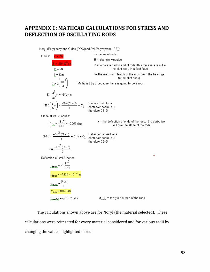
93
APPENDIX C: MATHCAD CALCULATIONS FOR STRESS AND DEFLECTION OF OSCILLATING RODS
The calculations shown above are for Noryl (the material selected). These
calculations were reiterated for every material considered and for various radii by
changing the values highlighted in red.

94
APPENDIX D: FINAL TANK DESIGN
This SolidWorks screen shot shows the overall test tank layout. The pumps pump the water
down the outer channels, where the water merges from the converger and travels through the
diffuser. The water is then fairly uniform at the testing area.
The blue arrows show the direction of
flow in the tank.
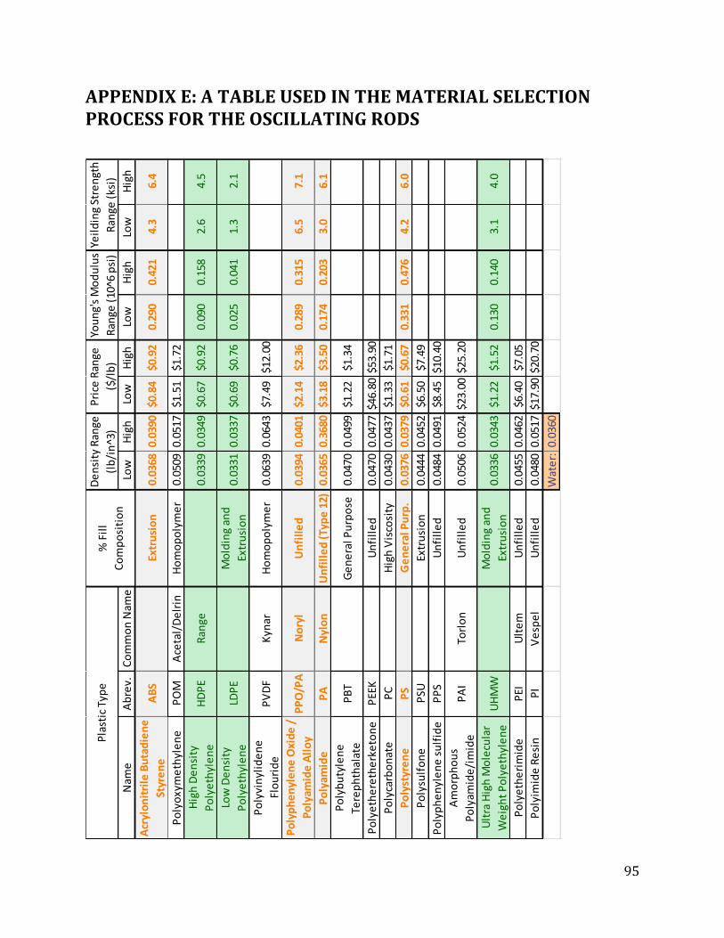
95
APPENDIX E: A TABLE USED IN THE MATERIAL SELECTION PROCESS FOR THE OSCILLATING RODS
Nam
eA
bre
v.C
om
mo
n N
ame
Low
Hig
hLo
wH
igh
Low
Hig
hLo
wH
igh
Acr
ylo
nit
rile
Bu
tad
ien
e
Styr
en
eA
BS
Extr
usi
on
0.03
680.
0390
$0.8
4$0
.92
0.29
00.
421
4.3
6.4
Po
lyo
xym
eth
yle
ne
PO
MA
ceta
l/D
elr
inH
om
op
oly
me
r0.
0509
0.05
17$1
.51
$1.7
2
Hig
h D
en
sity
Po
lye
thyl
en
eH
DP
ER
ange
0.03
390.
0349
$0.6
7$0
.92
0.09
00.
158
2.6
4.5
Low
De
nsi
ty
Po
lye
thyl
en
eLD
PE
Mo
ldin
g an
d
Extr
usi
on
0.03
310.
0337
$0.6
9$0
.76
0.02
50.
041
1.3
2.1
Po
lyvi
nyl
ide
ne
Flo
uri
de
PV
DF
Kyn
arH
om
op
oly
me
r0.
0639
0.06
43$7
.49
$12.
00
Po
lyp
he
nyl
en
e O
xid
e /
Po
lyam
ide
All
oy
PP
O/P
AN
ory
lU
nfi
lle
d0.
0394
0.04
01$2
.14
$2.3
60.
289
0.31
56.
57.
1
Po
lyam
ide
PA
Nyl
on
Un
fill
ed
(Ty
pe
12)
0.03
650.
3680
$3.1
8$3
.50
0.17
40.
203
3.0
6.1
Po
lyb
uty
len
e
Tere
ph
thal
ate
PB
TG
en
era
l Pu
rpo
se0.
0470
0.04
99$1
.22
$1.3
4
Po
lye
the
reth
erk
eto
ne
PEE
KU
nfi
lle
d0.
0470
0.04
77$4
6.80
$53.
90
Po
lyca
rbo
nat
eP
CH
igh
Vis
cosi
ty0.
0430
0.04
37$1
.33
$1.7
1
Po
lyst
yre
ne
PS
Ge
ne
ral P
urp
.0.
0376
0.03
79$0
.61
$0.6
70.
331
0.47
64.
26.
0
Po
lysu
lfo
ne
PSU
Extr
usi
on
0.04
440.
0452
$6.5
0$7
.49
Po
lyp
he
nyl
en
e s
ulf
ide
PP
SU
nfi
lle
d0.
0484
0.04
91$8
.45
$10.
40
Am
orp
ho
us
Po
lyam
ide
/im
ide
PA
ITo
rlo
nU
nfi
lle
d0.
0506
0.05
24$2
3.00
$25.
20
Ult
ra H
igh
Mo
lecu
lar
We
igh
t P
oly
eth
yle
ne
UH
MW
Mo
ldin
g an
d
Extr
usi
on
0.03
360.
0343
$1.2
2$1
.52
0.13
00.
140
3.1
4.0
Po
lye
the
rim
ide
PEI
Ult
em
Un
fill
ed
0.04
550.
0462
$6.4
0$7
.05
Po
lyim
ide
Re
sin
PI
Ve
spe
lU
nfi
lle
d0.
0480
0.05
17$1
7.90
$20.
70
Wat
er:
0.03
60
Pla
stic
Typ
eYe
ild
ing
Stre
ngt
h
Ran
ge (
ksi)
De
nsi
ty R
ange
(lb
/in
^3)
Pri
ce R
ange
($/l
b)
You
ng'
s M
od
ulu
s
Ran
ge (
10^6
psi
)%
Fil
l
Co
mp
osi
tio
n
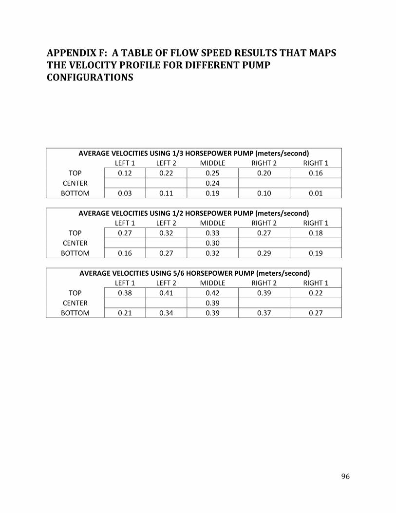
96
APPENDIX F: A TABLE OF FLOW SPEED RESULTS THAT MAPS THE VELOCITY PROFILE FOR DIFFERENT PUMP CONFIGURATIONS
AVERAGE VELOCITIES USING 1/3 HORSEPOWER PUMP (meters/second) LEFT 1 LEFT 2 MIDDLE RIGHT 2 RIGHT 1
TOP 0.12 0.22 0.25 0.20 0.16
CENTER 0.24
BOTTOM 0.03 0.11 0.19 0.10 0.01
AVERAGE VELOCITIES USING 1/2 HORSEPOWER PUMP (meters/second)
LEFT 1 LEFT 2 MIDDLE RIGHT 2 RIGHT 1
TOP 0.27 0.32 0.33 0.27 0.18
CENTER 0.30
BOTTOM 0.16 0.27 0.32 0.29 0.19
AVERAGE VELOCITIES USING 5/6 HORSEPOWER PUMP (meters/second)
LEFT 1 LEFT 2 MIDDLE RIGHT 2 RIGHT 1
TOP 0.38 0.41 0.42 0.39 0.22
CENTER 0.39
BOTTOM 0.21 0.34 0.39 0.37 0.27