Embed Size (px)
Citation preview
ASC Report No. 14/2012
Optimized Imex Runge-Kutta methods forsimulations in astrophysics: A detailed study
Inmaculada Higueras, Natalie Happenhofer, Othmar Koch, and
Friedrich Kupka
Institute for Analysis and Scientific Computing
Vienna University of Technology — TU Wien
www.asc.tuwien.ac.at ISBN 978-3-902627-05-6
Most recent ASC Reports
13/2012 H. WoracekAsymptotics of eigenvalues for a class of singular Krein strings
12/2012 H. Winkler, H. WoracekA growth condition for Hamiltonian systems related with Krein strings
11/2012 B. Schorkhuber, T. Meurer, and A. JungelFlatness-based trajectory planning for semilinear parabolic PDEs
10/2012 Michael Karkulik, David Pavlicek, and Dirk PraetoriusOn 2D newest vertex bisection: Optimality of mesh-closure and H1-stability ofL2-projection
09/2012 Joachim Schoberl and Christoph LehrenfeldDomain Decomposition Preconditioning for High Order Hybrid DiscontinuousGalerkin Methods on Tetrahedral Meshes
08/2012 Markus Aurada, Michael Feischl, Thomas Fuhrer, Michael Karkulik, Jens Mar-kus Melenk, Dirk PraetoriusClassical FEM-BEM coupling methods: nonlinearities, well-posedness, and ad-aptivity
07/2012 Markus Aurada, Michael Feischl, Thomas Fuhrer, Michael Karkulik, Jens MarkusMelenk, Dirk PraetoriusInverse estimates for elliptic integral operators and application to the adaptivecoupling of FEM and BEM
06/2012 J.M. Melenk, A. Parsania, and S. SauterGeneralized DG-Methods for Highly Indefinite Helmholtz Problems based on theUltra-Weak Variational Formulation
05/2012 J.M. Melenk, H. Rezaijafari, B. WohlmuthQuasi-optimal a priori estimates for fluxes in mixed finite element methods andapplications to the Stokes-Darcy coupling
04/2012 M. Langer, H. WoracekIndefinite Hamiltonian systems whose Titchmarsh-Weyl coefficients have no fi-nite generalized poles of non-negativity type
Institute for Analysis and Scientific ComputingVienna University of TechnologyWiedner Hauptstraße 8–101040 Wien, Austria
E-Mail: [email protected]
WWW: http://www.asc.tuwien.ac.at
FAX: +43-1-58801-10196
ISBN 978-3-902627-05-6
c© Alle Rechte vorbehalten. Nachdruck nur mit Genehmigung des Autors.
ASCTU WIEN
OPTIMIZED IMEX RUNGE–KUTTA METHODS FORSIMULATIONS IN ASTROPHYSICS: A DETAILED STUDY ∗
INMACULADA HIGUERAS† , NATALIE HAPPENHOFER‡ , OTHMAR KOCH§ , AND
FRIEDRICH KUPKA¶
Abstract. We construct and analyze strong stability preserving implicit–explicit Runge–Kuttamethods for the time integration of models of flow and radiative transport in astrophysical applica-tions. It turns out that in addition to the optimization of the region of absolute monotonicity, otherproperties of the methods are crucial for the success of the simulations as well. The models in ourfocus dictate to also take into account the step–size limits associated with dissipativity and positivityof the stiff parabolic terms which represent transport by diffusion. Another important property isuniform convergence of the numerical approximation with respect to different stiffness of those sameterms. Furthermore, it has been argued that in the presence of hyperbolic terms, the stability regionshould contain a large part of the imaginary axis even though the essentially non–oscillatory methodsused for the spatial discretization have eigenvalues with a negative real part. Hence, we constructseveral new methods which differ from each other by taking various or even all of these constraintssimultaneously into account. It is demonstrated for the problem of double–diffusive convection thatthe newly constructed schemes provide a significant computational advantage over methods from theliterature. They may also be useful for general problems which involve the solution of advection-diffusion equations, or other transport equations with similar stability requirements.
Key words. Runge–Kutta, implicit–explicit, total–variation–diminishing, strong stability pre-serving, hydrodynamics, stellar convection and pulsation, double–diffusive convection, numericalmethods.
AMS subject classifications. 65M06, 65M08, 65M20, 65L05.
1. Introduction. In this paper we discuss the construction of strong stabilitypreserving (SSP) implicit–explicit (IMEX) Runge–Kutta (RK) methods optimizedfor the deployment in radiation hydrodynamical simulations which are common invarious fields of astrophysics. Specifically, the associated models of flow and radiativetransport inside stars have the structure of advection–diffusion equations which canbe discretized in space by dissipative finite difference methods and essentially non–oscillatory (ENO) schemes, and subsequently propagated in time by Runge–Kuttamethods. Thus, we consider the ODE initial value problem
y(t) = F (y(t)) +G(y(t)), y(0) = y0, (1.1)
where we assume that the vector fields F and G have different stiffness properties. Forthis type of problems, additive Runge–Kutta schemes were demonstrated to improvethe efficiency of numerical simulations for the semiconvection problem in astrophysicsin [23]. These methods were constructed with the aim to optimize the region ofabsolute monotonicity. This region characterizes the step–sizes which are admissiblein order to ensure that the total variation (or some other suitable sublinear functional)
∗Supported by the Ministerio de Ciencia e Innovacion, project MTM2011–23203 and by theAustrian Science Fund (FWF), projects P21742–N16 and P20973†Universidad Publica de Navarra, Departamento de Ingenierıa Matematica e Informatica, Campus
de Arrosadia, 31006 Pamplona, Spain ([email protected]).‡University of Vienna, Faculty of Mathematics, Nordbergstraße 15, A–1090 Wien, Austria
([email protected]).§Vienna University of Technology, Institute for Analysis and Scientific Computing, A–1040 Wien,
Austria ([email protected]).¶University of Vienna, Faculty of Mathematics, Nordbergstraße 15, A–1090 Wien, Austria
1
2 Higueras et al.
of the spatial profile does not increase artificially in the course of time integration[11, 33]. In the case of the total–variation seminorm, this property is commonlyreferred to as total variation diminishing (TVD), or more generally as strong stabilitypreserving (SSP) (see, for example, [5, 6, 28]). In [23], it was demonstrated that forthe solution of the semiconvection problem, TVD IMEX methods from the literatureprovide a significant computational advantage and enhance the stability and accuracyof the simulations. Motivated by these observations the aim of the present paper isto construct new schemes which have additional properties beneficial to astrophysicalsimulations at the cost of reducing the region of absolute monotonicity from theoptimum. We will demonstrate that the new methods are overall more efficient andaccurate than methods used previously.
An analysis of the properties of TVD IMEX methods and experimental assess-ment of their performance [23] indicates that the following properties of the methodspromise reliable and efficient simulations:
• The IMEX scheme should be of second order. Furthermore, the error constantshould be small. Since the accuracy of such simulations is generally limited bythe spatial resolution, third order methods do not promise further advantages.
• The IMEX scheme should be SSP and it should have a large region of absolutemonotonicity [11, 12]. This implies that both the explicit and the implicitschemes are SSP. Furthermore, the Kraaijevanger radius (also known as theradius of absolute monotonicity) [21] of both schemes should also be large.
• The stability function of the implicit scheme should tend to zero at infinityand the stability region should contain a large subinterval of the negative realaxis [−z, 0] with z > 0. This is ensured by L–stability.
• For the explicit scheme, the stability region should contain large subintervalsof the negative real axis, [−z, 0] with z > 0, and also of the imaginary axis,[−w i, w i, ] with w > 0. The latter requirement is associated with a stableintegration of the hyperbolic advection terms (see [24, 36]).
• For both schemes, the stability function should be nonnegative for a largeinterval of the negative real axis, [−z, 0] with z > 0. This condition is di-rectly related to the step–size restrictions associated with the dissipativity ofthe spatial discretization [34] and should prevent spurious oscillations of thenumerical solution.
• The region of absolute stability of the IMEX scheme should be large. Inorder to be robust, it should also contain the curves studied in [2].
• For a convenient and memory–efficient implementation, the coefficients ofthe scheme should be rational numbers which could enable to recombine thestages in a suitable way.
The properties listed above turn out to be more important for a successful simula-tion than third order accuracy. Still, we cannot use the optimal SSP2(2,2,2) two–stagemethod [23], because the number of degrees of freedom does not allow to have a pos-itive stability function in conjunction with L–stability. Thus, we will focus on theconstruction of second–order three–stage IMEX RK schemes (A, A, bt) of the form
0 0 0 0
c2 a21 0 0
c3 a31 a32 0
A b1 b2 b3
c1 γ 0 0
c2 a21 γ 0
c3 a31 a32 γ
A b1 b2 b3
(1.2)
Optimized IMEX Methods for Simulations in Astrophysics: a detailed study 3
Observe the structural properties of this scheme: the weight vector b is the same forboth schemes, and the implicit scheme is a Singly Diagonally Implicit Runge–Kuttamethod (SDIRK). The first property implies that there are no extra coupling orderconditions for the IMEX scheme; that is, if both schemes have second order, the IMEXscheme also has second order [27]. Another advantage of IMEX schemes with b = bis that they preserve linear invariants of the ODE [15]. The second property is alsointeresting from the computational point of view because it allows to solve, stage tostage, the nonlinear systems that arise when implicit RK methods are used. Actually,the Jacobian matrix may even be frozen throughout the iterations for all the stages(see [8]). Imposing second order convergence leaves a total of seven degrees of freedomfor optimization as we explain below.
The rest of the paper is organized as follows. In §2, we review some knownresults that are used throughout the paper. Section 3 is devoted to the constructionof a second order 3–stage IMEX RK method with all the properties pointed out inthe introduction, amongst them, a nontrivial intersection of the stability region of theexplicit RK method and the imaginary axis. It turns out that this property of theexplicit scheme leads to an important decreasing of the stability interval, the intervalof nonnegativity of the stability function, and the Kraaijevanger coefficient. For thisreason, in §4 we construct IMEX RK methods whose implicit scheme is the optimalsecond order 3–stage SSP RK method. In addition, although the optimal secondorder 3–stage SSP SDIRK method is not L–stable, we also investigate properties ofIMEX RK methods constructed with this optimum SDIRK scheme; this study is donein §5 and §6. In order to test the constructed schemes for problems of our interest,the results of some numerical experiments are given in §7. Some conclusions are givenin §8. Finally, in order to help the reader, there is an appendix section that collectsthe most relevant properties of the methods constructed in this paper; in order tostress the advantages of the new methods, in the appendix section we also include theproperties of some methods from the literature.
The methods have been obtained with the help of the symbolic computationsoftware Mathematica.
2. Review of some known concepts. In this section we briefly review someknown concepts that are used along the paper.
2.1. Order of convergence. As we have pointed out above, the IMEX schemeshould achieve second order. To fulfill this requirement, the following conditionsshould be imposed (see for example [27]),
bte = 1 , btc =1
2, btc =
1
2, (2.1)
where, as usual, e = (1, . . . , 1)t and c = (c1, . . . , cs), c = (c1, . . . , cs); furthermore, wewill also assume that
A e = c , A e = c . (2.2)
We would like to stress at this point that problem parameters may affect themagnitude of the global error even if the expected convergence order is formallyretained. This is the case for problems of the form
y′ = F (y) +1
εG(y) , (2.3)
4 Higueras et al.
where ε� 1. Uniform convergence of IMEX RK methods applied to solve systems ofthe form (2.3) is studied in [1]. To obtain the results, in [1], the additive ODE (2.3)is transformed into a partitioned system of the form
y′ = f(y, z) ,
εz′ = g(y, z) .
It turns out that, if
btA−1c = 1 , (2.4)
then, for ε ≤ C ∆t, the global error satisfies
yn − y(tn) = O((∆t)p) +O(ε(∆t)2) , zn − z(tn) = O((∆t)2) ,
where p is the order of the explicit scheme; if conversely (2.4) is violated, the globalerror is of the form
yn − y(tn) = O((∆t)p) +O(ε∆t) , zn − z(tn) = O(∆t) .
2.2. Radius and regions of absolute monotonicity. For RK and IMEX RKmethods, step size restrictions to obtain SSP or TVD schemes are given, respectively,by the Kraaijevanger radius (or radius of absolute monotonicity) and the region ofabsolute monotonicity. The literature collects an extensive research on TVD and SSPRK methods [3, 4, 10, 11, 12, 13, 14, 17, 18, 21, 22, 26, 27, 28, 30, 31, 32, 33] (see[5, 7, 9, 29] for reviews on the topic).
An s–stage RK method (A, bt) is said to be absolutely monotonic at a given point−r, with r ≥ 0, if I + rA is nonsingular, and
(I + rA)−1A ≥ 0 , (I + rA)−1e ≥ 0 , (2.5)
where now e = (1, 1, . . . , 1)t ∈ Rs+1, A is defined by
A =
(A 0bt 0
),
and the inequalities in (2.5) are understood component–wise. The radius of absolutemonotonicity R(A) is defined by
R(A) = sup{ r | r ≥ 0 and A is absolutely monotonic on [−r, 0] } .
For RK methods, monotonicity can be ensured under a stepsize restriction of the form∆t ≤ τ0 ·R(A), where τ0 is the step size restriction for monotonicity when the explicitEuler method is used. For details see [21].
For additive RK methods, the concept of radius of absolute monotonicity is ex-tended to the region of absolute monotonicity [11, Definition 2.3] (see also [33]). Ans–stage additive RK method (A, A) is said to be absolutely monotonic (a.m.) at agiven point (−r1,−r2) with r1, r2 ≥ 0, if the matrix I + r1A + r2A is invertible,
(I + r1 A + r2 A)−1e ≥ 0, and
(I + r1 A + r2 A)−1
A ≥ 0 , (2.6)
(I + r1 A + r2 A)−1
A ≥ 0 . (2.7)
Optimized IMEX Methods for Simulations in Astrophysics: a detailed study 5
The region of absolute monotonicity, R(A, A), is defined by
R(A, A) = { (r1, r2) | r1 ≥ 0 , r2 ≥ 0 and (A, A) is a.m. on [−r1, 0]× [−r2, 0] } .
Numerical monotonicity can be ensured for the additive RK method (A, A) under thestepsize restriction ∆t ≤ min {r1 τ0, r2 τ0}, where r1 and r2 are such that the point(r1, r2) ∈ R(A, A), and τ0, τ0 > 0 are the step size restrictions for monotonicity whenthe explicit Euler method is used for F and G, respectively (see [11] for details).
Consequently, in order to obtain nontrivial step size restrictions for RK and ad-ditive RK methods, we should have, respectively, R(A) > 0, and points (r1, r2) ∈R(A, A) with r1 > 0 and r2 > 0. In [11, 21], algebraic criteria for nontrivial radiusand regions of absolute monotonicity are given in terms of sign conditions of the coef-ficient matrix (or matrices), namely, A ≥ 0 (or A ≥ 0, A ≥ 0), and some inequalitiesof the incidence matrix of certain matrices. A trivial way to ensure these propertiesfor IMEX schemes is to impose
aij , aij > 0 for i < j , bj , bj > 0 , and γ > 0 . (2.8)
For this reason, for the IMEX RK schemes constructed in this paper we will assumethe positivity conditions (2.8).
2.3. Amplification function for second order 3–point and fourth or-der 5–point spatial discretization. In order to study the stability of numericalschemes, we can study the dissipativity of time integrators in conjunction with spa-tial discretizations by means of Fourier analysis [16]. For the dissipativity analysis ofadvection–diffusion equations, it is sufficient to consider only the diffusion term sincethe advection term becomes negligible in the limit where the spatial discretizationparameter tends to zero [34]. We thus consider the heat equation ut + a uxx = 0 andthe second order 3–point spatial discretization
uxx(xj , tn) ≈unj+1 − 2unj + unj−1
(4x)2,
and the fourth order 5–point spatial discretization
uxx(xj , tn) ≈−unj+2 + 16unj+1 − 30unj + 16unj−1 − unj−2
(4x)2.
These are two of the spatial discretizations actually implemented in the ANTARESsimulation code, which numerically solves the equations of hydrodynamics and variousgeneralizations thereof [25, 23].
When these spatial discretizations are used to solve the heat equation, the stabilityfunction R(z) of the RK method (A, bt), defined by
R(z) = 1 + z bt(I − zA)−1e ,
is evaluated at a point of the form z = −µh(θ), where µ ≥ 0, and h : [−π, π] → R,depends on the discretization considered. The function h satisfies h(z) > 0 for z ∈[−π, π], z 6= 0, and, due to the consistency of the spatial discretization, it also has theproperty h(0) = 0. We thus obtain the amplification function
g(µ, θ) = R(−µh(θ)) . (2.9)
6 Higueras et al.
Observe that R(0) = 1 implies g(µ, 0) = 1. In particular, for the second order 3–pointand for the fourth order 5–point spatial discretizations we obtain, respectively, thefollowing functions h3 and h5,
h3(θ) = −(e−i θ − 2 + ei θ) = 4 sin2
(θ
2
), (2.10)
h5(θ) = − 1
12
(16e−i θ + 16ei θ − e−2iθ − e2i θ − 30
)=
2
3(7− cos(θ)) sin2
(θ
2
). (2.11)
Since the functions h in (2.10) and (2.11) are even, h(θ) = h(−θ), we subsequentlyrestrict the values of θ to θ ∈ [0, π].
In the dissipativity analysis we are interested in the values:a) µ0 such that, for µ ∈ [0, µ0], it holds that g(µ, θ) > 0 for θ ∈ [0, π], andb) µ1 such that, for µ ∈ [0, µ1], it holds that |g(µ, θ)| ≤ 1 for θ ∈ [0, π] .
If µi =∞, i = 0, 1, we will understand that the interval [0, µi] is [0, µi).It turns out that, if z0 is the first negative zero of R(z), from the definition of
g(µ , θ) in (2.9) we obtain that
h(θ)µ = −z0 , θ ∈ [0, π] .
The lowest value µ0 is given by
µ0 = − z0
maxθ∈[0,π] h(θ).
In a similar way, if z1 is the first negative zero of |R(z)| − 1, we obtain that
h(θ)µ = −z1 , θ ∈ [0, π] .
The lowest value µ1 is given by
µ1 = − z1
maxθ∈[0,π] h(θ).
Observe that [z1, 0] is the stability interval of the RK method, that is, the intersectionof the stability region with the real axis. In particular, for the 3–points and for the5–points discretizations, as hi is monotonic, we get
maxθ∈[0,π]
h3(θ) = h3(π) = 4 , maxθ∈[0,π]
h5(θ) = h5(π) =16
3.
Consequently, for each RK method, in the dissipativity analysis, it is enough to com-pute z0, the first negative zero of R(z), and z1, the first strictly negative zero of thefunction |R(z)| − 1. For each spatial discretization, the values µ0 and µ1 are simplyscaled values of |z0| and |z1|, respectively, and thus, for our purpose, the larger |z0|and |z1|, the better.
3. A new second order 3 stages SSP IMEX scheme. In this section weconstruct a new second order 3 stages SSP IMEX scheme of the form (1.2) with allthe requirements explained in §1. We begin constructing the explicit scheme and, ina second step, we will deal with the implicit one. Finally, we will fix the remainingfree parameters to obtain the desired properties for the IMEX scheme.
Optimized IMEX Methods for Simulations in Astrophysics: a detailed study 7
3.1. Explicit scheme. Condition (2.2) and second order conditions (2.1) forthe explicit scheme lead to
b1 = 1− b2 − b3 , c3 =1− 2 b2 c2
2 b3, a21 = c2 , a31 = c3 − a32 . (3.1)
Hence, four degrees of freedom of the explicit scheme are left to be determined afterthe previous considerations. For a second order 3–stage explicit scheme, the stabilityfunction is given by [8]
R(z) = 1 + z +z2
2+ b3 a32 c2 z
3 .
Thus, defining
a32 =α
b3 c2, (3.2)
we obtain the stability function
R(z) = 1 + z +z2
2+ α z3. (3.3)
To express the four degrees of freedom, in the following we choose α, c2, b2, and b3.In the next subsection, we study the stability function (3.3) and the stability regionS in terms of α.
3.1.1. Stability function for the explicit scheme. We study the stabilityfunction (3.3) to determine the values of α such that the method fulfills all the desiredrequirements.
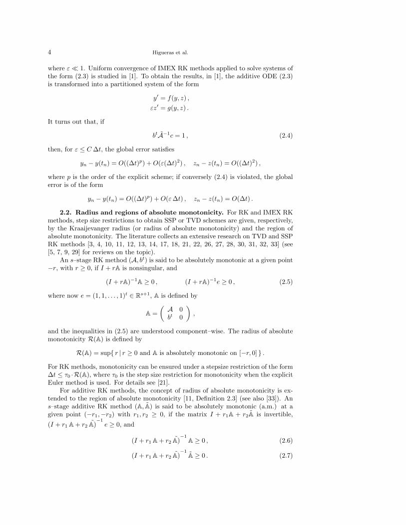
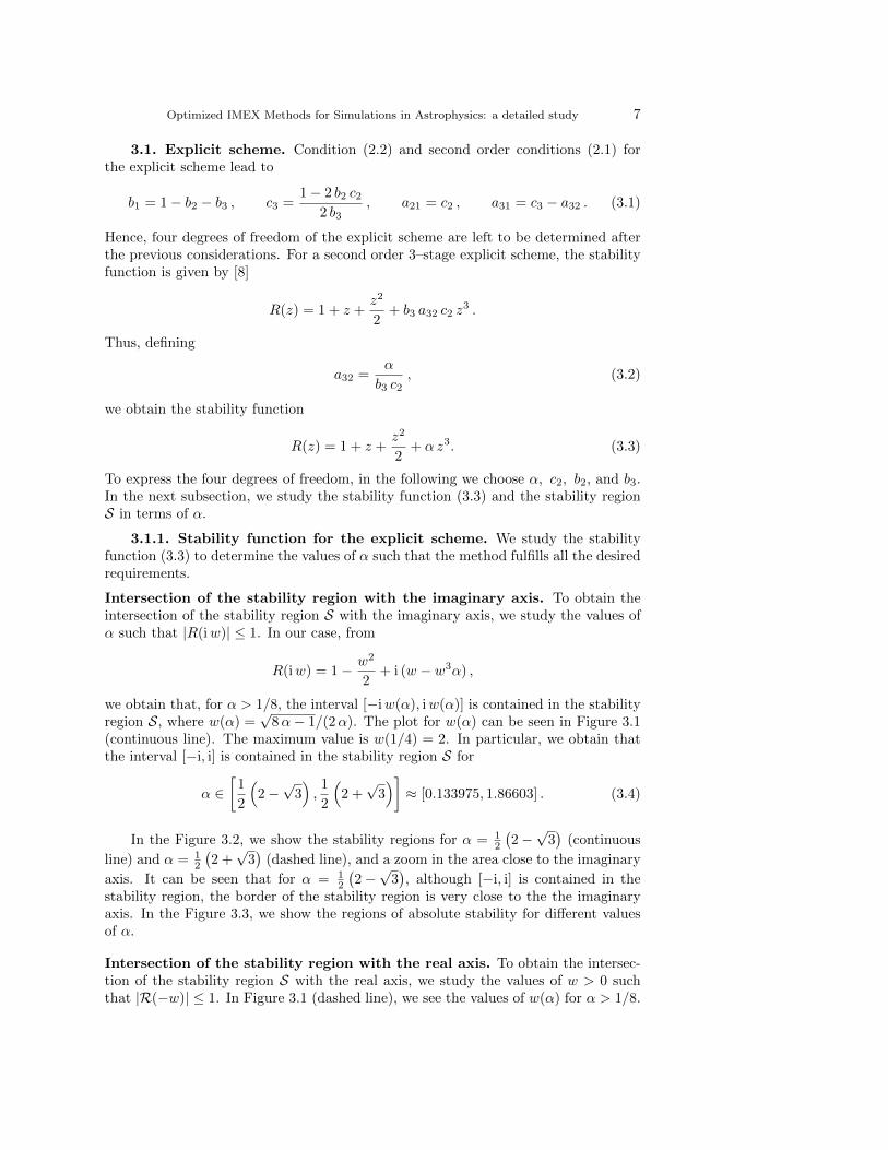
Intersection of the stability region with the imaginary axis. To obtain theintersection of the stability region S with the imaginary axis, we study the values ofα such that |R(iw)| ≤ 1. In our case, from
R(iw) = 1− w2
2+ i (w − w3α) ,
we obtain that, for α > 1/8, the interval [−iw(α), iw(α)] is contained in the stabilityregion S, where w(α) =
√8α− 1/(2α). The plot for w(α) can be seen in Figure 3.1
(continuous line). The maximum value is w(1/4) = 2. In particular, we obtain thatthe interval [−i, i] is contained in the stability region S for
α ∈[
1
2
(2−√
3),
1
2
(2 +√
3)]≈ [0.133975, 1.86603] . (3.4)
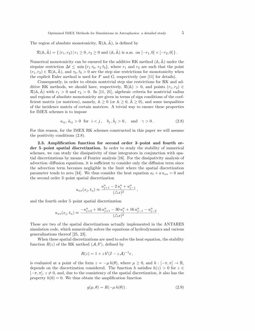
In the Figure 3.2, we show the stability regions for α = 12
(2−√
3)
(continuous
line) and α = 12
(2 +√
3)
(dashed line), and a zoom in the area close to the imaginary
axis. It can be seen that for α = 12
(2−√
3), although [−i, i] is contained in the
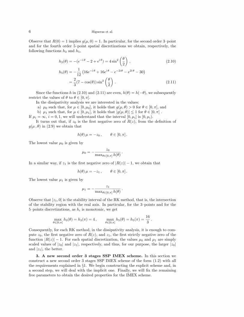
stability region, the border of the stability region is very close to the the imaginaryaxis. In the Figure 3.3, we show the regions of absolute stability for different valuesof α.
Intersection of the stability region with the real axis. To obtain the intersec-tion of the stability region S with the real axis, we study the values of w > 0 suchthat |R(−w)| ≤ 1. In Figure 3.1 (dashed line), we see the values of w(α) for α > 1/8.
8 Higueras et al.
0.5 1.0 1.5 2.0 2.5 3.0Α
0.5
1.0
1.5
2.0
2.5
3.0
w
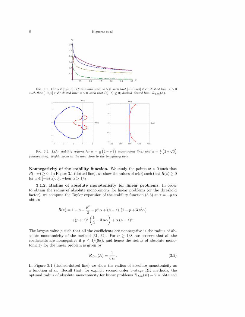
Fig. 3.1. For α ∈ [1/8, 3]. Continuous line: w > 0 such that [−w i, w i] ∈ S; dashed line: z > 0such that [−z, 0] ∈ S; dotted line: z > 0 such that R(−z) ≥ 0; dashed–dotted line: RLin(A).
-3 -2 -1 0 1-3
-2
-1
0
1
2
3
ReHzL
ImHzL
-0.010 -0.005 0.000 0.005 0.010-0.2
-0.1
0.0
0.1
0.2
ReHzL
ImHzL
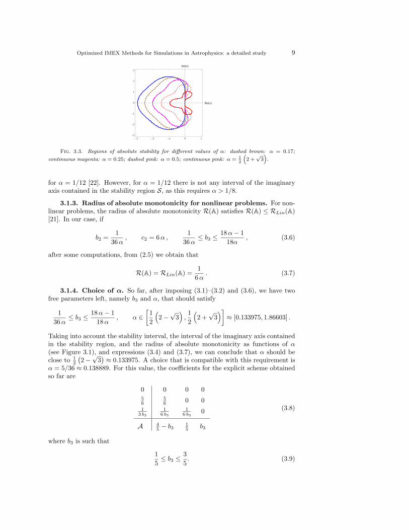
Fig. 3.2. Left: stability regions for α = 12
(2−√
3)
(continuous line) and α = 12
(2 +√
3)
(dashed line). Right: zoom in the area close to the imaginary axis.
Nonnegativity of the stability function. We study the points w > 0 such thatR(−w) ≥ 0. In Figure 3.1 (dotted line), we show the values of w(α) such that R(z) ≥ 0for z ∈ [−w(α), 0], when α > 1/8.
3.1.2. Radius of absolute monotonicity for linear problems. In orderto obtain the radius of absolute monotonicity for linear problems (or the thresholdfactor), we compute the Taylor expansion of the stability function (3.3) at x = −p toobtain
R(z) = 1− p+p2
2− p3 α+ (p+ z)
(1− p+ 3 p2α
)+(p+ z)2
(1
2− 3 pα
)+ α (p+ z)3 .
The largest value p such that all the coefficients are nonnegative is the radius of ab-solute monotonicity of the method [31, 32]. For α ≥ 1/8, we observe that all thecoefficients are nonnegative if p ≤ 1/(6α), and hence the radius of absolute mono-tonicity for the linear problem is given by
RLin(A) =1
6α. (3.5)
In Figure 3.1 (dashed-dotted line) we show the radius of absolute monotonicity asa function of α. Recall that, for explicit second order 3–stage RK methods, theoptimal radius of absolute monotonicity for linear problems RLin(A) = 2 is obtained
Optimized IMEX Methods for Simulations in Astrophysics: a detailed study 9
-3 -2 -1 0 1-3
-2
-1
0
1
2
3
ReHzL
ImHzL
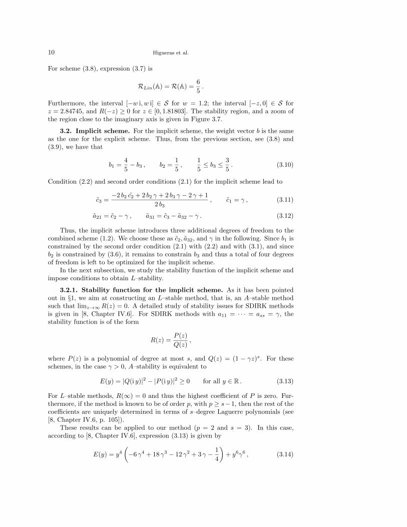
Fig. 3.3. Regions of absolute stability for different values of α: dashed brown: α = 0.17;
continuous magenta: α = 0.25; dashed pink: α = 0.5; continuous pink: α = 12
(2 +√
3)
.
for α = 1/12 [22]. However, for α = 1/12 there is not any interval of the imaginaryaxis contained in the stability region S, as this requires α > 1/8.
3.1.3. Radius of absolute monotonicity for nonlinear problems. For non-linear problems, the radius of absolute monotonicity R(A) satisfies R(A) ≤ RLin(A)[21]. In our case, if
b2 =1
36α, c2 = 6α ,
1
36α≤ b3 ≤
18α− 1
18α, (3.6)
after some computations, from (2.5) we obtain that
R(A) = RLin(A) =1
6α. (3.7)
3.1.4. Choice of α. So far, after imposing (3.1)–(3.2) and (3.6), we have twofree parameters left, namely b3 and α, that should satisfy
1
36α≤ b3 ≤
18α− 1
18α, α ∈
[1
2
(2−√
3),
1
2
(2 +√
3)]≈ [0.133975, 1.86603] .
Taking into account the stability interval, the interval of the imaginary axis containedin the stability region, and the radius of absolute monotonicity as functions of α(see Figure 3.1), and expressions (3.4) and (3.7), we can conclude that α should beclose to 1
2
(2−√
3)≈ 0.133975. A choice that is compatible with this requirement is
α = 5/36 ≈ 0.138889. For this value, the coefficients for the explicit scheme obtainedso far are
0 0 0 056
56 0 0
13 b3
16 b3
16 b3
0
A 45 − b3
15 b3
(3.8)
where b3 is such that
1
5≤ b3 ≤
3
5. (3.9)
10 Higueras et al.
For scheme (3.8), expression (3.7) is
RLin(A) = R(A) =6
5.
Furthermore, the interval [−w i, w i] ∈ S for w = 1.2; the interval [−z, 0] ∈ S forz = 2.84745, and R(−z) ≥ 0 for z ∈ [0, 1.81803]. The stability region, and a zoom ofthe region close to the imaginary axis is given in Figure 3.7.
3.2. Implicit scheme. For the implicit scheme, the weight vector b is the sameas the one for the explicit scheme. Thus, from the previous section, see (3.8) and(3.9), we have that
b1 =4
5− b3 , b2 =
1
5,
1
5≤ b3 ≤
3
5. (3.10)
Condition (2.2) and second order conditions (2.1) for the implicit scheme lead to
c3 =−2 b2 c2 + 2 b2 γ + 2 b3 γ − 2 γ + 1
2 b3, c1 = γ , (3.11)
a21 = c2 − γ , a31 = c3 − a32 − γ . (3.12)
Thus, the implicit scheme introduces three additional degrees of freedom to thecombined scheme (1.2). We choose these as c2, a32, and γ in the following. Since b1 isconstrained by the second order condition (2.1) with (2.2) and with (3.1), and sinceb2 is constrained by (3.6), it remains to constrain b3 and thus a total of four degreesof freedom is left to be optimized for the implicit scheme.
In the next subsection, we study the stability function of the implicit scheme andimpose conditions to obtain L–stability.
3.2.1. Stability function for the implicit scheme. As it has been pointedout in §1, we aim at constructing an L–stable method, that is, an A–stable methodsuch that limz→∞R(z) = 0. A detailed study of stability issues for SDIRK methodsis given in [8, Chapter IV.6]. For SDIRK methods with a11 = · · · = ass = γ, thestability function is of the form
R(z) =P (z)
Q(z),
where P (z) is a polynomial of degree at most s, and Q(z) = (1 − γz)s. For theseschemes, in the case γ > 0, A–stability is equivalent to
E(y) = |Q(i y)|2 − |P (i y)|2 ≥ 0 for all y ∈ R . (3.13)
For L–stable methods, R(∞) = 0 and thus the highest coefficient of P is zero. Fur-thermore, if the method is known to be of order p, with p ≥ s−1, then the rest of thecoefficients are uniquely determined in terms of s–degree Laguerre polynomials (see[8, Chapter IV.6, p. 105]).
These results can be applied to our method (p = 2 and s = 3). In this case,according to [8, Chapter IV.6], expression (3.13) is given by
E(y) = y4
(−6 γ4 + 18 γ3 − 12 γ2 + 3 γ − 1
4
)+ y6γ6 , (3.14)
Optimized IMEX Methods for Simulations in Astrophysics: a detailed study 11
0.5 1.0 1.5 2.0Γ
0.001
0.01
0.1
1
Log ÈCÈ
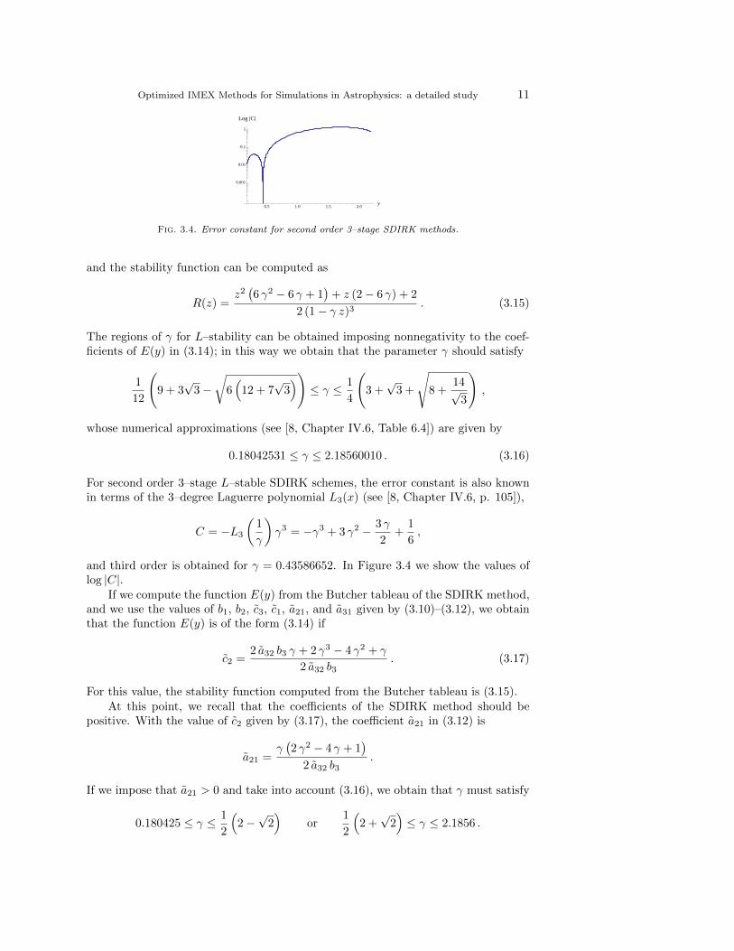
Fig. 3.4. Error constant for second order 3–stage SDIRK methods.
and the stability function can be computed as
R(z) =z2(6 γ2 − 6 γ + 1
)+ z (2− 6 γ) + 2
2 (1− γ z)3. (3.15)
The regions of γ for L–stability can be obtained imposing nonnegativity to the coef-ficients of E(y) in (3.14); in this way we obtain that the parameter γ should satisfy
1
12
(9 + 3
√3−
√6(
12 + 7√
3))≤ γ ≤ 1
4
(3 +√
3 +
√8 +
14√3
),
whose numerical approximations (see [8, Chapter IV.6, Table 6.4]) are given by
0.18042531 ≤ γ ≤ 2.18560010 . (3.16)
For second order 3–stage L–stable SDIRK schemes, the error constant is also knownin terms of the 3–degree Laguerre polynomial L3(x) (see [8, Chapter IV.6, p. 105]),
C = −L3
(1
γ
)γ3 = −γ3 + 3 γ2 − 3 γ
2+
1
6,
and third order is obtained for γ = 0.43586652. In Figure 3.4 we show the values oflog |C|.
If we compute the function E(y) from the Butcher tableau of the SDIRK method,and we use the values of b1, b2, c3, c1, a21, and a31 given by (3.10)–(3.12), we obtainthat the function E(y) is of the form (3.14) if
c2 =2 a32 b3 γ + 2 γ3 − 4 γ2 + γ
2 a32 b3. (3.17)
For this value, the stability function computed from the Butcher tableau is (3.15).At this point, we recall that the coefficients of the SDIRK method should be
positive. With the value of c2 given by (3.17), the coefficient a21 in (3.12) is
a21 =γ(2 γ2 − 4 γ + 1
)2 a32 b3
.
If we impose that a21 > 0 and take into account (3.16), we obtain that γ must satisfy
0.180425 ≤ γ ≤ 1
2
(2−√
2)
or1
2
(2 +√
2)≤ γ ≤ 2.1856 .
12 Higueras et al.
As 12
(2−√
2)≈ 0.29289322 and 1
2
(2 +√
2)≈ 1.70710678, taking into account the
size of the error constant (see Figure 3.4), we restrict the values of γ for L–stabilityin (3.16) to
0.18042531 ≤ γ ≤ 0.29289322 . (3.18)
Note that this interval does not contain the value of γ for which the scheme wouldbe of third order.
With regard to the intersection of the real and imaginary axis with the stabilityregion, observe that, as the method is L–stable, the imaginary axis as well as the realaxis is contained in the stability region S. It remains to study the nonnegativity ofthe stability function.
We analyze now if there is any value of γ such that R(z) ≥ 0 for all z < 0. Weobtain a positive answer for
γ ∈(
0,1
3
(3−√
6)]≈ (0, 0.18350342] . (3.19)
Combining this result with (3.18), we get that adequate values for γ are
0.18042531 ≤ γ ≤ 0.18350342 . (3.20)
3.2.2. Radius of absolute monotonicity for linear problems. For linearproblems, the computation of the radius of absolute monotonicity for implicit schemesis not an easy task. To obtain it, we have to find the points z such that the stabilityfunction R is absolutely monotonic at z. Recall that a function f is said to beabsolutely monotonic at a given point x ∈ R if f (k)(x) exist and f (k)(x) ≥ 0 fork ≥ 0. For explicit methods, the stability function R is a polynomial, and thus,we can analyze a finite number of derivatives to check if the function is absolutelymonotonic at a given point x. However, for implicit schemes, R is a rational function,and we cannot use directly the definition of absolute monotonicity.
In this section, we apply Theorem 4.4 in [35] to obtain the radius of absolutemonotonicity for linear problems for our SDIRK method. Roughly speaking, thisresult allows us to restrict the analysis to a finite number of derivatives, that is,R(k)(x) ≥ 0 for 0 ≤ k < K(x), and the key point is to obtain the integer K(x). Inthe following proposition we compute it for the stability function (3.15).
Proposition 3.1. Assume that γ satisfies (3.20), γ 6=(3−√
6)/3. If R(k)(x) ≥
0 for k = 0, 1, 2, 3, then the stability function (3.15) is absolutely monotonic at x.Proof. In order to apply [35, Theorem 4.4], we construct all the elements (sets,intervals, functions, etc.) involved in this result. Following the notation in [35], thestability function (3.15) is of the form R(z) = P (z)/Q(z) with
P (z) = z2
(3 γ2 − 3 γ +
1
2
)+ z (1− 3 γ) + 1 , Q(z) = γ3
(1
γ− z)3
.
The polynomials P and Q have degrees m = 2 and n = 3, respectively, and there is aunique pole α0 = 1/γ > 0 with multiplicity µ(α0) = 3. Thus the set A = A+ = {α0},I(α0) = R, and B(R(z)) =∞. Next, the stability function should be decomposed inpartial fractions of the form
R(z) = c(α0, 1)1
α0 − z+ c(α0, 2)
1
(α0 − z)2+ c(α0, 3)
1
(α0 − z)3.

Optimized IMEX Methods for Simulations in Astrophysics: a detailed study 13
0.1810 0.1815 0.1820 0.1825 0.1830 0.1835Γ
1
2
3
4
5
6
x
Fig. 3.5. From bottom to top, values of −x such that condition (3.21) holds for k = 1, 2, 3, 4.
In our case,
c(α0, 1) =6 γ2 − 6 γ + 1
2 γ3, c(α0, 2) =
−3 γ2 + 5 γ − 1
γ4, c(α0, 3) =
2 γ2 − 4 γ + 1
2 γ5.
For γ satisfying (3.20), γ 6=(3−√
6)/3, these functions have constant sign. More
precisely, c(α0, 1) ≥ 0, c(α0, 2) ≤ 0, and c(α0, 3) > 0. Now, we construct the function(see [35, Formula (4.2)])
F (k, x) =2 c(α0, 1) k!
(k + 2)!
(1
γ− x)2
− 2 c(α0, 2) (k + 1)!
(k + 2)!
∣∣∣∣ 1γ − x∣∣∣∣ ,
where we have used the sign conditions of c(α0, 1) and c(α0, 2). Another functionneeded to construct K(x) in [35] is L(x); in our case, L(x) = 0, see [35, Formula(4.3)]. We can now construct the integer K(x) in [35, Definition 4.1]), defined as thesmallest integer k such that k ≥ L(x) and
F (k, x) < |c(α0, 3)| . (3.21)
For γ satisfying (3.20), in Figure 3.5 we show, from bottom to top, the values of−x such that condition (3.21) holds for k = 1, 2, 3, 4. We do not consider k = 0because, as we have seen in the previous subsection (see (3.19)), for the values of γsatisfying (3.20), it holds that R(z) ≥ 0 for z ≤ 0. Furthermore, we restrict the valuesto −x ∈ [0, 6] because, by numerical search, it has been found that the nonlinearoptimum radius of absolute monotonicity for second order 3–stage SDIRK schemes is6 [4, 19]. Consequently, for −x ∈ [0, 6], K(x) ≤ 4. We can now apply Theorem 4.4in [35] to ensure that R(z) is absolutely monotonic in [x, 0] if and only if c(α0, 3) > 0and R(k)(x) ≥ 0 for 0 ≤ k < K(x). Thus, the next step is to analyze the values of xsuch that R(k)(x) ≥ 0 for k = 0, 1, 2, 3. �
For each γ satisfying (3.20), the radius of absolute monotonicity is given by
R(γ) =1− 4 γ
γ (6 γ2 − 6 γ + 1)−
√−12 γ3 + 28 γ2 − 10 γ + 1
γ2 (6 γ2 − 6 γ + 1)2 , (3.22)
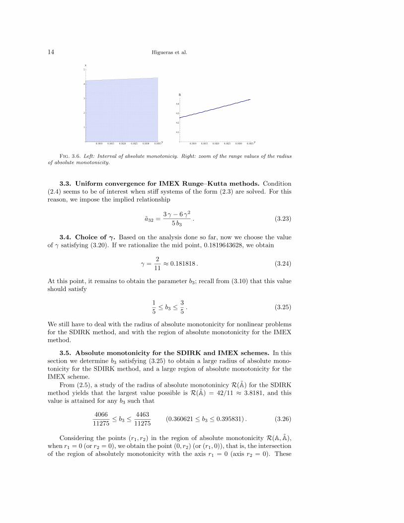
and varies in the interval [4.25512, 4.44949]. In Figure 3.6 we show, for each γ, theinterval of absolute monotonicity, and a zoom of the value range of the radius ofabsolute monotonicity. We observe that, for the different values of γ, the radius ofabsolute monotonicity does not change significantly.
14 Higueras et al.
0.1810 0.1815 0.1820 0.1825 0.1830 0.1835Γ
1
2
3
4
5
x
0.1810 0.1815 0.1820 0.1825 0.1830 0.1835Γ
4.1
4.2
4.3
4.4
R
Fig. 3.6. Left: Interval of absolute monotoniciy. Right: zoom of the range values of the radiusof absolute monotonicity.
3.3. Uniform convergence for IMEX Runge–Kutta methods. Condition(2.4) seems to be of interest when stiff systems of the form (2.3) are solved. For thisreason, we impose the implied relationship
a32 =3 γ − 6 γ2
5 b3. (3.23)
3.4. Choice of γ. Based on the analysis done so far, now we choose the valueof γ satisfying (3.20). If we rationalize the mid point, 0.1819643628, we obtain
γ =2
11≈ 0.181818 . (3.24)
At this point, it remains to obtain the parameter b3; recall from (3.10) that this valueshould satisfy
1
5≤ b3 ≤
3
5. (3.25)
We still have to deal with the radius of absolute monotonicity for nonlinear problemsfor the SDIRK method, and with the region of absolute monotonicity for the IMEXmethod.
3.5. Absolute monotonicity for the SDIRK and IMEX schemes. In thissection we determine b3 satisfying (3.25) to obtain a large radius of absolute mono-tonicity for the SDIRK method, and a large region of absolute monotonicity for theIMEX scheme.
From (2.5), a study of the radius of absolute monotoninicy R(A) for the SDIRKmethod yields that the largest value possible is R(A) = 42/11 ≈ 3.8181, and thisvalue is attained for any b3 such that
4066
11275≤ b3 ≤
4463
11275(0.360621 ≤ b3 ≤ 0.395831) . (3.26)
Considering the points (r1, r2) in the region of absolute monotonicity R(A, A),when r1 = 0 (or r2 = 0), we obtain the point (0, r2) (or (r1, 0)), that is, the intersectionof the region of absolutely monotonicity with the axis r1 = 0 (axis r2 = 0). These
Optimized IMEX Methods for Simulations in Astrophysics: a detailed study 15
values satisfy r2 ≤ R(A), r1 ≤ R(A). Quite often, due to the mixed conditions (2.6)for r1 = 0, and (2.7) for r2 = 0, that is,
(I + r2 A)−1
A ≥ 0 , (I + r1 A)−1 A ≥ 0 ,
we obtain r2 < R(A) and r1 < R(A). We aim for determining the largest valuesof r2 and r1 such that the points (r1, 0) and (0, r2) belong to the region of absolutemonotonicity.
A detailed study yields the result that the largest value of r2 such that (0, r2) ∈R(A, A) is r2 = 66/43 ≈ 1.53488, provided that
1
5≤ b3 ≤
1462
3025(0.2 ≤ b3 ≤ 0.483306) . (3.27)
In a similar way, the largest value of r1 such that (r1, 0) ∈ R(A, A) is r1 = 126/55 ≈2.29091, provided that
1
5≤ b3 ≤
109616
213565(0.2 ≤ b3 ≤ 0.513268) . (3.28)
Taking into account (3.26), (3.27), and (3.28), we consider
b3 =4
11≈ 0.363636 . (3.29)
By fixing this value, we have finished the construction of the IMEX scheme.
3.6. Second order 3–stage SSP IMEX scheme (summary). In this sec-tion, we give the coefficients of the IMEX scheme obtained from our earlier consider-ations, that is
0 0 0 056
56 0 0
1112
1124
1124 0
A 2455
15
411
211
211 0 0
289462
205462
211 0
751924
20334620
21110
211
A 2455
15
411
(3.30)
and summarize its properties.This is a second order IMEX scheme such that the implicit method is L–stable.
The stability functions for the explicit and implicit schemes are
RA(z) = 1 + z +z2
2+
5
36z3 , RA(z) =
11(13 z2 + 110 z + 242
)2 (11− 2 z)3
. (3.31)
In Figure 3.7, we show the stability regions for the explicit and the implicit schemesin (3.30), as well as a zoom of the region in a neighborhood of the origin. In Figure3.8, we show the stability region of the IMEX scheme and a zoom of the region at theorigin.
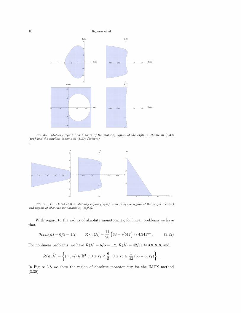
For the explicit scheme, we obtain R(z) ≥ 0 for z ∈ [−1.81803, 0], and |R(z)| ≤ 1for z ∈ [−2.84745, 0]. Furthermore, |R(iw)| ≤ 1 for w ∈ [−1.2, 1.2].
For the implicit scheme, R(z) ≥ 0 and |R(z)| ≤ 1 for z ≤ 0. Furthermore,|R(iw)| ≤ 1 for w ∈ R.
This IMEX method satisfies condition (2.4) for uniform convergence.
16 Higueras et al.
-5 -4 -3 -2 -1 1ReHzL
-3
-2
-1
1
2
3
ImHzL
-0.04 -0.02 0.02 0.04ReHzL
-2
-1
1
2
ImHzL
-20 -10 10 20ReHzL
-20
-10
10
20
ImHzL
-0.04 -0.02 0.02 0.04ReHzL
-2
-1
1
2
ImHzL
Fig. 3.7. Stability region and a zoom of the stability region of the explicit scheme in (3.30)(top) and the implicit scheme in (3.30) (bottom)
.
-50 -40 -30 -20 -10z
-15
-10
-5
5
10
15
w
-0.04 -0.02 0.02 0.04z
-2
-1
1
2
w
0.5 1.0 1.5 2.0r1
0.5
1.0
1.5
r2
Fig. 3.8. For IMEX (3.30): stability region (right), a zoom of the region at the origin (center)and region of absolute monotonicity (right).
With regard to the radius of absolute monotonicity, for linear problems we havethat
RLin(A) = 6/5 = 1.2, RLin(A) =11
26
(33−
√517)≈ 4.34177 . (3.32)
For nonlinear problems, we have R(A) = 6/5 = 1.2, R(A) = 42/11 ≈ 3.81818, and
R(A, A) =
{(r1, r2) ∈ R2 : 0 ≤ r1 <
6
5, 0 ≤ r2 ≤
1
43(66− 55 r1)
}.
In Figure 3.8 we show the region of absolute monotonicity for the IMEX method(3.30).
Optimized IMEX Methods for Simulations in Astrophysics: a detailed study 17
Due to the properties listed above, we will refer to scheme (3.30) as SSP2(3,3,2)–LSPUM, where the letters have the following meanings:
’L’: L–stable;’S’: the stability region for the explicit part contains an interval
on the imaginary axis;’P’: the amplification factor g is always positive;’U’: the IMEX method features uniform convergence (2.4);’M’: the IMEX method has a nontrivial region of absolute monotonicity.
(3.33)
To assess the merits of the method just constructed, in the next section we willconstruct alternative schemes based on optimal methods from the literature. Thesewill be compared experimentally in §7.
4. IMEX methods with second order 3–stage optimum SSP explicit RKscheme as explicit method. In this section, we construct a number of additionalSSP IMEX methods, based on the optimal explicit three–stage second–order methodin conjunction with a compatible implicit scheme. These will be compared to thescheme constructed in Section 3. Thus, we consider IMEX schemes of the form
0 0 0 012
12 0 0
1 12
12 0
A 13
13
13
c1 γ 0 0
c2 a21 γ 0
c3 a31 a32 γ
A 13
13
13
(4.1)
The explicit method coincides with the explicit scheme for the SSP2(3,3,2) schemesin [11, 27]. Observe that now, the weight vector b for the implicit scheme is alreadyfixed. Recalling the discussion from §3.2, we note that this leaves only three degreesof freedom for the scheme (4.1), namely, c2, a32, and γ.
For the implicit schemes considered in this section, we will impose L–stabilityand the nonnegativity of the stability function R(z) for all z ≤ 0. As the stabilityfunction for an L–stable second order 3–stage SDIRK method only depends on thediagonal elements γ, the study conducted in §3.2.1 is valid and, therefore, we chooseagain γ = 2/11.
Furthermore, after imposing second order conditions for the implicit scheme, anda stability function of the form (3.15), c2 is also determined, and we obtain that thereis one free parameter left: a32. In this section, we construct three schemes by choosingthis value as follows:
1. In the first one, we impose condition (2.4) for uniform convergence, see §4.1.2. In the second one, we optimize the radius of absolute monotonicity of the
SDIRK scheme, see §4.2.3. In the third one, we optimize the region of absolute monotonicity of the IMEX
scheme, see §4.3.
4.1. IMEX method with uniform convergence (2.4). In this case, theIMEX scheme obtained by imposing (2.4) is given by the coefficient tableaux
0 0 0 012
12 0 0
1 12
12 0
A 13
13
13
211
211 0 0
69154
41154
211 0
6777
289847
42121
211
A 13
13
13
(4.2)
18 Higueras et al.
-50 -40 -30 -20 -10z
-15
-10
-5
5
10
15
w
-0.04 -0.02 0.02 0.04z
-2
-1
1
2
w
0.5 1.0 1.5 2.0r1
0.5
1.0
1.5
r2
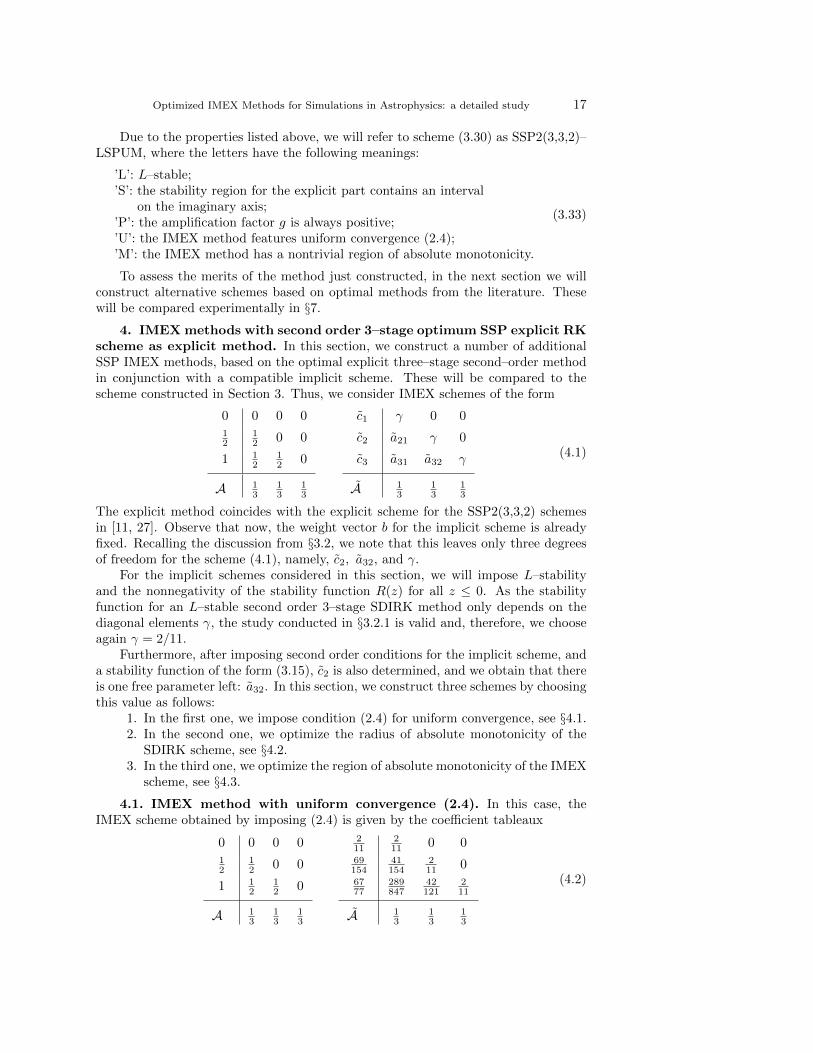
Fig. 4.1. For the IMEX method (4.2): Left: Stability region; center: zoom of the stabilityregion; right: region of absolute monotonicity.
This method satisfies condition (2.4) for uniform convergence. Note that (3.23) mustnot be reused to derive (4.2), because (3.23) has been derived assuming (3.10) whereb2 = 1/5 instead of b2 = 1/3.
Recalling (3.2) and (3.3), the stability function for the explicit scheme is
RA(z) = 1 + z +1
2z2 +
1
12z3 , (4.3)
whereas for the implicit scheme it is given by RA(z) in (3.31), since it depends onlyon γ (see (3.15)).
For linear problems, the radius of absolute monotonicity for the explicit schemeis RLin(A) = 2, whereas for the implicit scheme RLin(A) is given by (3.32). Fornonlinear problems, the explicit scheme is the optimal second order 3–stage explicitSSP method and thus R(A) = 2; for the implicit method, from (2.5), we get
R(A) =1694
275 +√
74701≈ 3.08947 .
For the IMEX scheme,
R(A, A) ={(r1, r2) ∈ R2 : 0 ≤ r1 <
1
24
(308− 117 r1 −
√37√
213 r21 − 1320 r1 + 1936
)}.
The points (0, 1.6816) and (2, 0) are included in the region of absolute monotonic-ity R(A, A). In Figure 4.1 we show the stability region and the region of absolutemonotonicity of the IMEX scheme. Due to its properties, we will henceforth refer tomethod (4.2) as SSP2(3,3,2)–LPUM (see (3.33)).
4.2. IMEX scheme with large radius of absolute monotonicity R(A) .A detailed study shows that the largest value for R(A) is 3.85824, and that this valueis attained for a32 = 0.3039. We rationalize this number to obtain
a32 =7
23≈ 0.304348 .
We thus obtain the IMEX scheme
0 0 0 012
12 0 0
1 12
12 0
A 13
13
13
211
211 0 0
45239317
28299317
211 0
1551718634
148529428582
723
211
A 13
13
13
(4.4)
Optimized IMEX Methods for Simulations in Astrophysics: a detailed study 19
-50 -40 -30 -20 -10z
-15
-10
-5
5
10
15
w
-0.04 -0.02 0.02 0.04z
-2
-1
1
2
w
0.5 1.0 1.5 2.0r1
0.5
1.0
1.5
r2
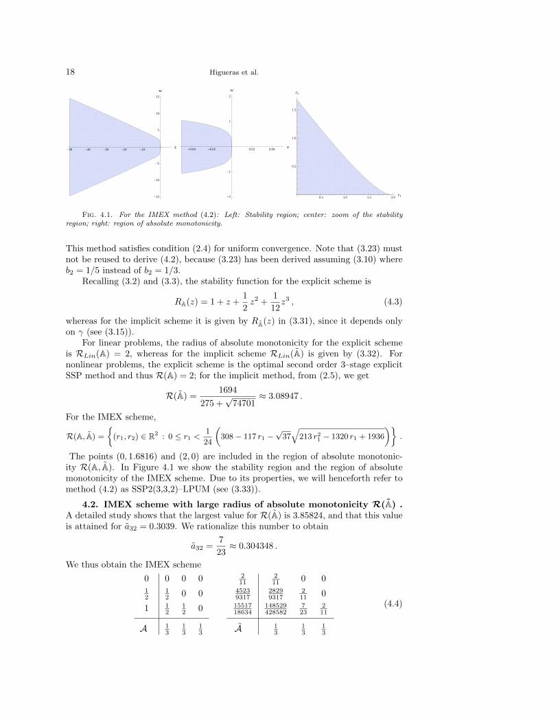
Fig. 4.2. For the IMEX method (4.4): Left: Stability region; center: zoom of the stabilityregion; right: region of absolute monotonicity.
We remark that this method does not satisfy condition (2.4) for uniform convergence.The stability functions for the explicit and implicit RK methods in (4.4) are given by(4.3) and (3.31), respectively.
For linear problems, the radius of absolute monotonicity for the explicit schemeis RLin(A) = 2, whereas for the implicit scheme RLin(A) is given by (3.32). Fornonlinear problems, the explicit scheme is the optimal second order 3–stage explicitSSP method and thus R(A) = 2; for the implicit method, we have
R(A) =11(5353−
√18761649
)2920
≈ 3.84822 .
For the IMEX scheme,
R(A, A) ={(r1, r2) ∈ R2 : 0 ≤ r1 < −
11
76(223r1 − 644)− 33
76
√11√
467r21 − 2760r1 + 4048
}.
The points (0, 1.5849) and (2, 0) are included in the region of absolute monotonic-ity R(A, A). In Figure 4.2 we show the stability region and the region of absolutemonotonicity for the IMEX scheme.
4.3. IMEX scheme with large region of absolute monotonicity. A de-tailed study shows that the largest value of r2 such that (0, r2) ∈ R(A, A) is r2 =2.34236; this value is attained for a32 = 0.47635. We rationalize this number to obtainthat for
a32 =10
21≈ 0.47619 ,
we have that the point (0, r2) is in the region of absolute monotonicity for
r2 =11(√
9242421− 2641)
1874≈ 2.34284 .
We thus obtain the IMEX scheme
0 0 0 012
12 0 0
1 12
12 0
A 13
13
13
211
211 0 0
500313310
258313310
211 0
62716655
39731139755
1021
211
A 13
13
13
(4.5)
20 Higueras et al.
-50 -40 -30 -20 -10z
-15
-10
-5
5
10
15
w
-0.04 -0.02 0.02 0.04z
-2
-1
1
2
w
0.5 1.0 1.5 2.0r1
0.5
1.0
1.5
2.0
2.5
r2
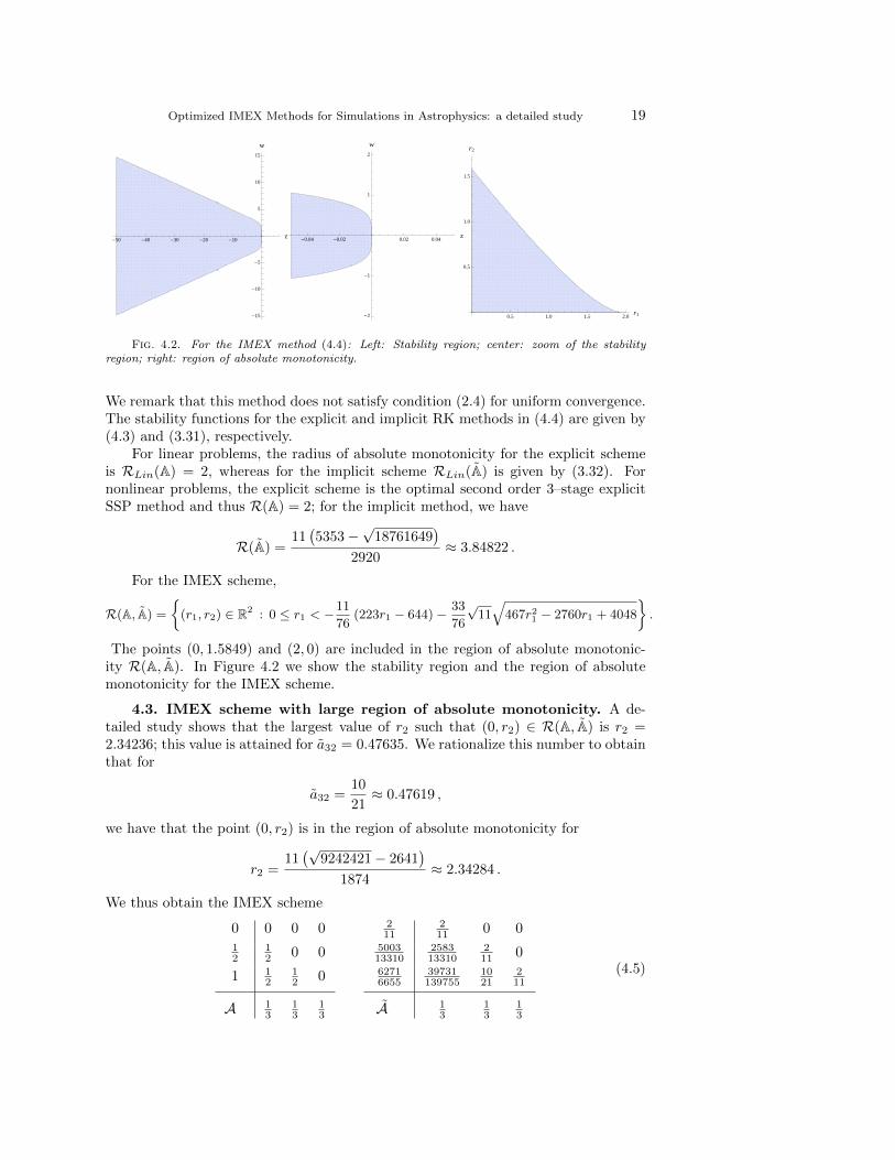
Fig. 4.3. For the IMEX method (4.5): Left: Stability region; center: zoom of the stabilityregion; right: region of absolute monotonicity.
We remark that this method does not satisfy conditon (2.4) for uniform convergence.The stability functions for the explicit and implicit RK methods in (4.5) are givenby (4.3) and (3.31), respectively. In Figure 4.3 we show the stability region for theIMEX scheme.
For the implicit scheme,
R(A) =11(√
9242421− 2641)
1874≈ 2.34284 .
For the IMEX scheme, the region of absolute monotonicity is shown in Figure 4.3.The points (0, 2.34033) and (2, 0) are included in the region of absolute monotonicityR(A, A). We will later refer to this scheme as SSP2(3,3,2)–LPM (see (3.33)).
5. IMEX scheme with optimal explicit SSP RK and optimal SSP SDIRKSSP methods. In this section we analyze the IMEX method constructed with theoptimal explicit and implicit 3–stage SSP methods,
0 0 0 012
12 0 0
1 12
12 0
A 13
13
13
16
16 0 0
12
13
16 0
56
13
13
16
A 13
13
13
(5.1)
This is a second order IMEX method such that b = b. The explicit part is theoptimal three–stage explicit SSP method of second order [21], while the implicit partrepresents the optimal three–stage scheme [3, 4, 19]. The stability function for theexplicit scheme is given by (4.3), while for the implicit scheme it is (see, e.g., [20])
RA(z) =(z + 6)3
(6− z)3. (5.2)
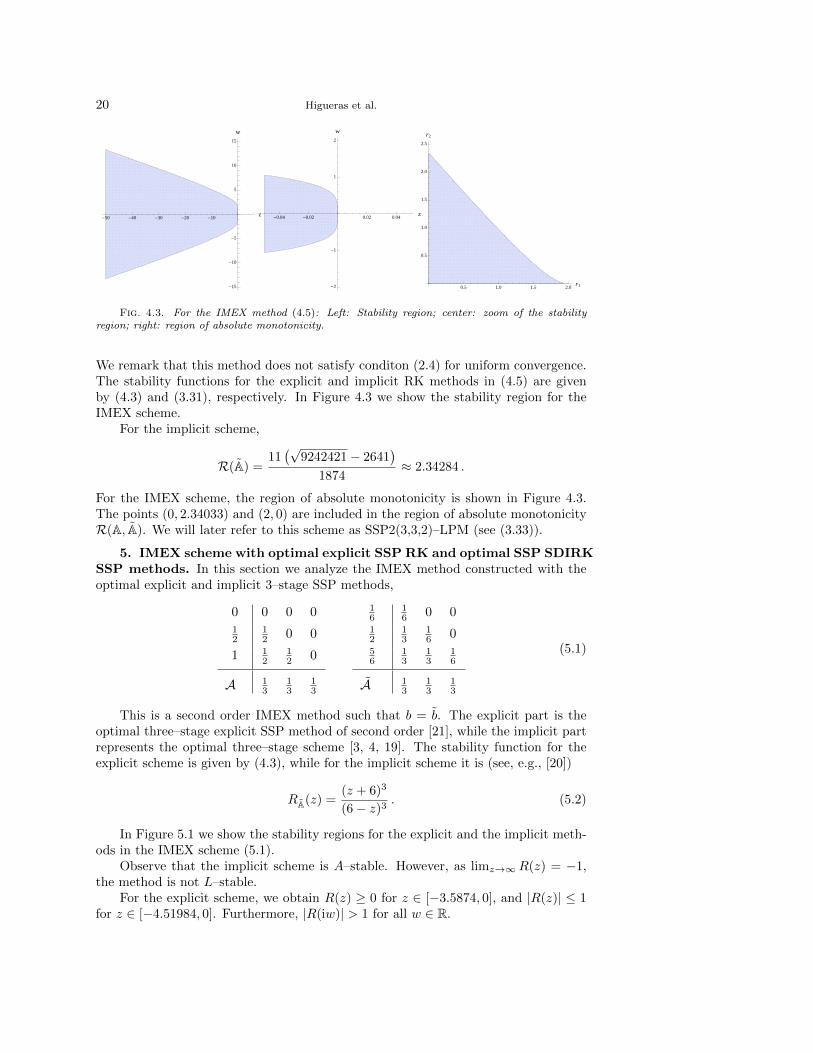
In Figure 5.1 we show the stability regions for the explicit and the implicit meth-ods in the IMEX scheme (5.1).
Observe that the implicit scheme is A–stable. However, as limz→∞R(z) = −1,the method is not L–stable.
For the explicit scheme, we obtain R(z) ≥ 0 for z ∈ [−3.5874, 0], and |R(z)| ≤ 1for z ∈ [−4.51984, 0]. Furthermore, |R(iw)| > 1 for all w ∈ R.
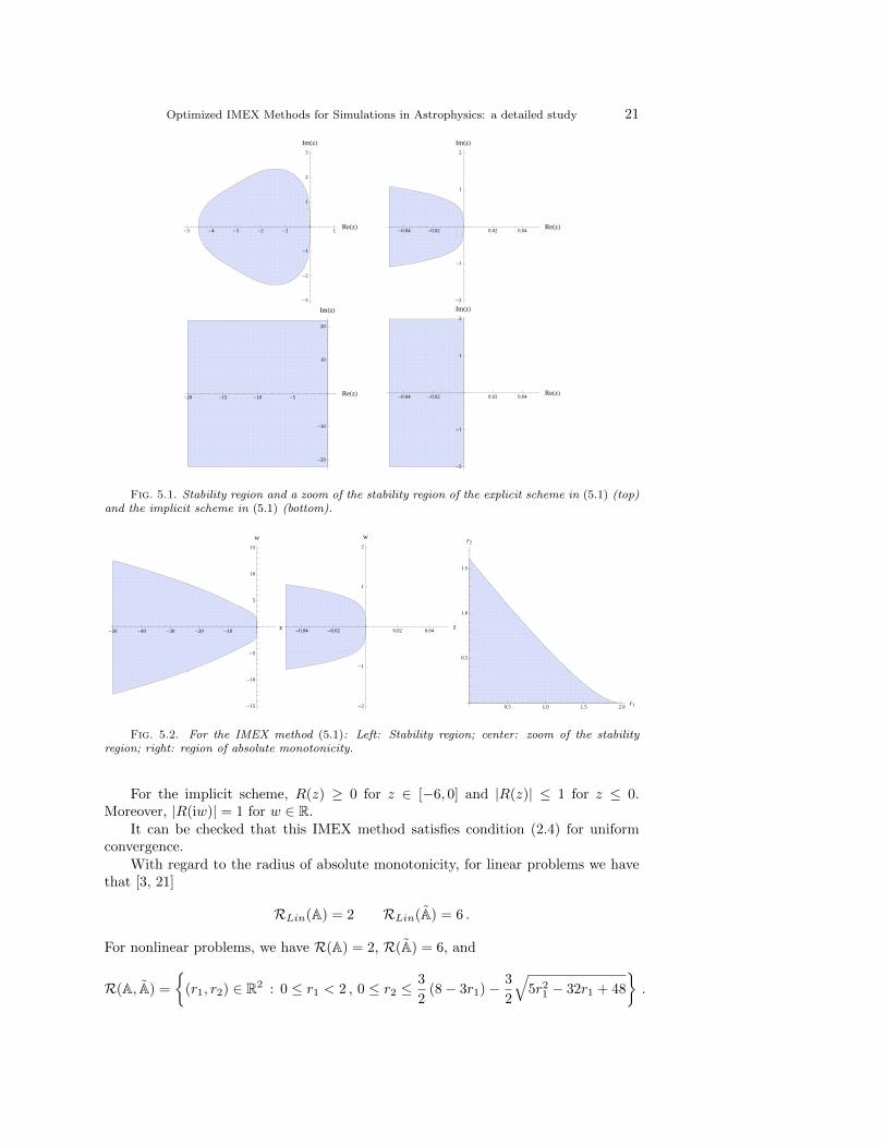
Optimized IMEX Methods for Simulations in Astrophysics: a detailed study 21
-5 -4 -3 -2 -1 1ReHzL
-3
-2
-1
1
2
3
ImHzL
-0.04 -0.02 0.02 0.04ReHzL
-2
-1
1
2
ImHzL
-20 -15 -10 -5ReHzL
-20
-10
10
20
ImHzL
-0.04 -0.02 0.02 0.04ReHzL
-2
-1
1
2
ImHzL
Fig. 5.1. Stability region and a zoom of the stability region of the explicit scheme in (5.1) (top)and the implicit scheme in (5.1) (bottom).
-50 -40 -30 -20 -10z
-15
-10
-5
5
10
15
w
-0.04 -0.02 0.02 0.04z
-2
-1
1
2
w
0.5 1.0 1.5 2.0r1
0.5
1.0
1.5
r2
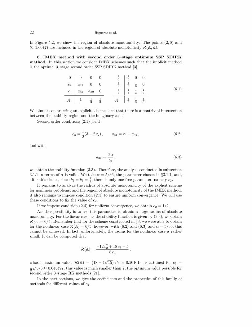
Fig. 5.2. For the IMEX method (5.1): Left: Stability region; center: zoom of the stabilityregion; right: region of absolute monotonicity.
For the implicit scheme, R(z) ≥ 0 for z ∈ [−6, 0] and |R(z)| ≤ 1 for z ≤ 0.Moreover, |R(iw)| = 1 for w ∈ R.
It can be checked that this IMEX method satisfies condition (2.4) for uniformconvergence.
With regard to the radius of absolute monotonicity, for linear problems we havethat [3, 21]
RLin(A) = 2 RLin(A) = 6 .
For nonlinear problems, we have R(A) = 2, R(A) = 6, and
R(A, A) =
{(r1, r2) ∈ R2 : 0 ≤ r1 < 2 , 0 ≤ r2 ≤
3
2(8− 3r1)− 3
2
√5r2
1 − 32r1 + 48
}.
22 Higueras et al.
In Figure 5.2, we show the region of absolute monotonicity. The points (2, 0) and(0, 1.6077) are included in the region of absolute monotonicity R(A, A).
6. IMEX method with second order 3–stage optimum SSP SDIRKmethod. In this section we consider IMEX schemes such that the implicit methodis the optimal 3–stage second order SSP SDIRK method [3],
0 0 0 0
c2 a21 0 0
c3 a31 a32 0
A 13
13
13
16
16 0 0
12
13
16 0
56
13
13
16
A 13
13
13
(6.1)
We aim at constructing an explicit scheme such that there is a nontrivial intersectionbetween the stability region and the imaginary axis.
Second order conditions (2.1) yield
c3 =1
2(3− 2 c2) , a31 = c3 − a32 , (6.2)
and with
a32 =3α
c2, (6.3)
we obtain the stability function (3.3). Therefore, the analysis conducted in subsection3.1.1 in terms of α is valid. We take α = 5/36, the parameter chosen in §3.1.1, and,after this choice, since b2 = b3 = 1
3 , there is only one free parameter, namely c2.
It remains to analyze the radius of absolute monotonicity of the explicit schemefor nonlinear problems, and the region of absolute monotonicity of the IMEX method;it also remains to impose condition (2.4) to ensure uniform convergence. We will usethese conditions to fix the value of c2.
If we impose condition (2.4) for uniform convergence, we obtain c2 = 1/2.
Another possibility is to use this parameter to obtain a large radius of absolutemonotonicity. For the linear case, as the stability function is given by (3.3), we obtainRLin = 6/5. Remember that for the scheme constructed in §3, we were able to obtainfor the nonlinear case R(A) = 6/5; however, with (6.2) and (6.3) and α = 5/36, thiscannot be achieved. In fact, unfortunately, the radius for the nonlinear case is rathersmall. It can be computed that
R(A) =−12 c22 + 18 c2 − 5
5 c2,
whose maximum value, R(A) =(18− 4
√15)/5 ≈ 0.501613, is attained for c2 =
12
√5/3 ≈ 0.645497; this value is much smaller than 2, the optimum value possible for
second order 3–stage RK methods [21].
In the next sections, we give the coefficients and the properties of this family ofmethods for different values of c2.
Optimized IMEX Methods for Simulations in Astrophysics: a detailed study 23
-50 -40 -30 -20 -10z
-15
-10
-5
5
10
15
w
-0.04 -0.02 0.02 0.04z
-2
-1
1
2
w
0.5 1.0 1.5 2.0r1
0.5
1.0
1.5
r2
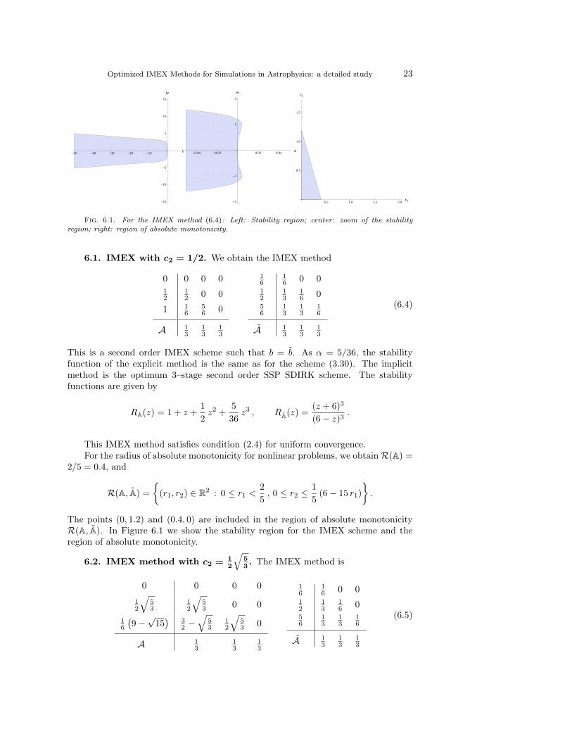
Fig. 6.1. For the IMEX method (6.4): Left: Stability region; center: zoom of the stabilityregion; right: region of absolute monotonicity.
6.1. IMEX with c2 = 1/2. We obtain the IMEX method
0 0 0 012
12 0 0
1 16
56 0
A 13
13
13
16
16 0 0
12
13
16 0
56
13
13
16
A 13
13
13
(6.4)
This is a second order IMEX scheme such that b = b. As α = 5/36, the stabilityfunction of the explicit method is the same as for the scheme (3.30). The implicitmethod is the optimum 3–stage second order SSP SDIRK scheme. The stabilityfunctions are given by
RA(z) = 1 + z +1
2z2 +
5
36z3 , RA(z) =
(z + 6)3
(6− z)3.
This IMEX method satisfies condition (2.4) for uniform convergence.For the radius of absolute monotonicity for nonlinear problems, we obtainR(A) =
2/5 = 0.4, and
R(A, A) =
{(r1, r2) ∈ R2 : 0 ≤ r1 <
2
5, 0 ≤ r2 ≤
1
5(6− 15 r1)
}.
The points (0, 1.2) and (0.4, 0) are included in the region of absolute monotonicityR(A, A). In Figure 6.1 we show the stability region for the IMEX scheme and theregion of absolute monotonicity.
6.2. IMEX method with c2 = 12
√53. The IMEX method is
0 0 0 0
12
√53
12
√53 0 0
16
(9−√
15)
32 −
√53
12
√53 0
A 13
13
13
16
16 0 0
12
13
16 0
56
13
13
16
A 13
13
13
(6.5)
24 Higueras et al.
-100 -80 -60 -40 -20ReHzL
-5
5
ImHzL
-0.04 -0.02 0.02 0.04ReHzL
-2
-1
1
2
ImHzL
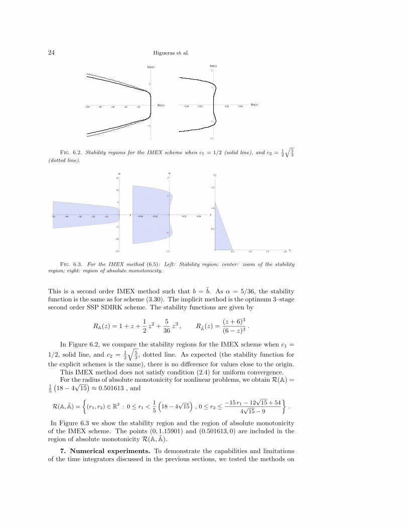
Fig. 6.2. Stability regions for the IMEX scheme when c1 = 1/2 (solid line), and c2 = 12
√53
(dotted line).
-50 -40 -30 -20 -10z
-15
-10
-5
5
10
15
w
-0.04 -0.02 0.02 0.04z
-2
-1
1
2
w
0.5 1.0 1.5 2.0r1
0.5
1.0
1.5
r2
Fig. 6.3. For the IMEX method (6.5): Left: Stability region; center: zoom of the stabilityregion; right: region of absolute monotonicity.
This is a second order IMEX method such that b = b. As α = 5/36, the stabilityfunction is the same as for scheme (3.30). The implicit method is the optimum 3–stagesecond order SSP SDIRK scheme. The stability functions are given by
RA(z) = 1 + z +1
2z2 +
5
36z3 , RA(z) =
(z + 6)3
(6− z)3.
In Figure 6.2, we compare the stability regions for the IMEX scheme when c1 =
1/2, solid line, and c2 = 12
√53 , dotted line. As expected (the stability function for
the explicit schemes is the same), there is no difference for values close to the origin.This IMEX method does not satisfy condition (2.4) for uniform convergence.For the radius of absolute monotonicity for nonlinear problems, we obtainR(A) =
15
(18− 4
√15)≈ 0.501613 , and
R(A, A) ={(r1, r2) ∈ R2 : 0 ≤ r1 <
1
5
(18− 4
√15), 0 ≤ r2 ≤
−15 r1 − 12√15 + 54
4√15− 9
}.
In Figure 6.3 we show the stability region and the region of absolute monotonicityof the IMEX scheme. The points (0, 1.15901) and (0.501613, 0) are included in theregion of absolute monotonicity R(A, A).
7. Numerical experiments. To demonstrate the capabilities and limitationsof the time integrators discussed in the previous sections, we tested the methods on
Optimized IMEX Methods for Simulations in Astrophysics: a detailed study 25
Method ∆tmax ∆tmean CFLmax CFLmean CFLstart Time
SSP2(2,2,2)–37.02 s 19.45 s 2.00 1.05 0.4 01:41:42
PM, γ=0.24
SSP2(3,3,2)–93.15 s 57.16 s 5.02 3.08 0.5 01:34:17
LUM
SSP2(3,3,2)–88.91 s 71.63 s 4.77 3.85 0.35 01:29:25
LSPUM
SSP2(3,3,2)–101.62 s 77.79 s 5.46 4.18 0.4 01:25:43
LPUM
SSP2(3,3,2)–56.48 s 38.36 s 3.03 2.06 0.25 01:46:22
LPM
SSP1(1,1,1)–9.32 s 1.22 s 0.5 0.07 0.05 —
LPMTable 7.1
Simulation A: Time–steps, CFL–numbers and wallclocktimes over the first 80 scrt.
simulations of double–diffusive convection in an idealized setting performed with thehydrodynamics code ANTARES [25]. Since the ANTARES code and the setting aredescribed in detail in [23], we will restrict ourselves to the results. The challenge ofthese simulations is that they require the time integration method to work for quitedifferent conditions within a single simulation run: only a method which can handlestiff terms and is also SSP can succeed with acceptable time–steps.
In this section we test the schemes named SSP2(3,3,2)–LSPUM, SSP2(3,3,2)–LPUM, and SSP2(3,3,2)–LPM, whose coefficients are given by (3.30), (4.2), and (4.5),respectively. For the meaning of the notation L–S–P–U–M, we refer to (3.33).
7.1. Simulation A. This setting corresponds to Simulation 1 in [23], namely,we assume a Prandtl number Pr = 0.1, a Lewis number Le = 0.1, a modified Rayleighnumber Ra∗ = 1.6 ∗ 105, and a stability parameter Rρ = 1.1. The simulations wererun on the Vienna Scientific Cluster (VSC) 1 on 64 CPUs.
To demonstrate the merits of the methods constructed in this paper, we also giveresults for the method IMEX SSP1(1,1,1), which is a combination of the forward andbackward Euler methods (see (9.1)). It becomes clear that such a simple low orderscheme is not advisable for our purposes. For a better comparison, we also list thebest performing schemes of [23], namely the SSP2(2,2,2) scheme with γ = 0.24 andthe SSP2(3,3,2) method, whose coefficients are given in (9.2), and (9.3), respectively.According to the notation introduced in this paper, see (3.33), we will refer to thesemethods as SSP1(1,1,1)–LPM, SSP2(2,2,2)–PM, and SSP2(3,3,2)–LUM.
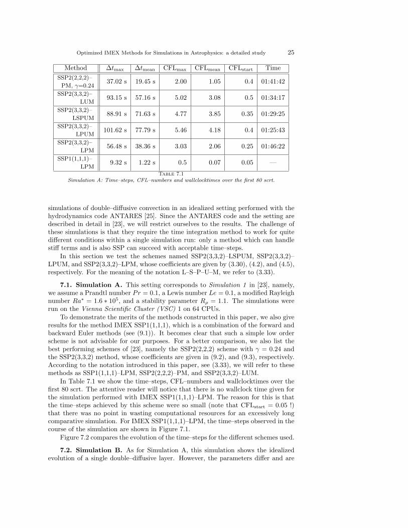
In Table 7.1 we show the time–steps, CFL–numbers and wallclocktimes over thefirst 80 scrt. The attentive reader will notice that there is no wallclock time given forthe simulation performed with IMEX SSP1(1,1,1)–LPM. The reason for this is thatthe time–steps achieved by this scheme were so small (note that CFLstart = 0.05 !)that there was no point in wasting computational resources for an excessively longcomparative simulation. For IMEX SSP1(1,1,1)–LPM, the time–steps observed in thecourse of the simulation are shown in Figure 7.1.
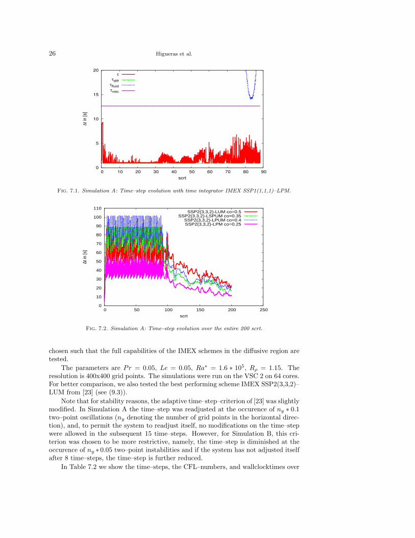
Figure 7.2 compares the evolution of the time–steps for the different schemes used.
7.2. Simulation B. As for Simulation A, this simulation shows the idealizedevolution of a single double–diffusive layer. However, the parameters differ and are
26 Higueras et al.
0
5
10
15
20
0 10 20 30 40 50 60 70 80 90
∆t
in [
s]
scrt
τ
τdiff
τfluid
τvisc
Fig. 7.1. Simulation A: Time–step evolution with time integrator IMEX SSP1(1,1,1)–LPM.
0
10
20
30
40
50
60
70
80
90
100
110
0 50 100 150 200 250
∆t in
[s]
scrt
SSP2(3,3,2)-LUM co=0.5SSP2(3,3,2)-LSPUM co=0.35
SSP2(3,3,2)-LPUM co=0.4SSP2(3,3,2)-LPM co=0.25
Fig. 7.2. Simulation A: Time–step evolution over the entire 200 scrt.
chosen such that the full capabilities of the IMEX schemes in the diffusive region aretested.
The parameters are Pr = 0.05, Le = 0.05, Ra∗ = 1.6 ∗ 105, Rρ = 1.15. Theresolution is 400x400 grid points. The simulations were run on the VSC 2 on 64 cores.For better comparison, we also tested the best performing scheme IMEX SSP2(3,3,2)–LUM from [23] (see (9.3)).
Note that for stability reasons, the adaptive time–step–criterion of [23] was slightlymodified. In Simulation A the time–step was readjusted at the occurence of ny ∗ 0.1two–point oscillations (ny denoting the number of grid points in the horizontal direc-tion), and, to permit the system to readjust itself, no modifications on the time–stepwere allowed in the subsequent 15 time–steps. However, for Simulation B, this cri-terion was chosen to be more restrictive, namely, the time–step is diminished at theoccurence of ny ∗ 0.05 two–point instabilities and if the system has not adjusted itselfafter 8 time–steps, the time–step is further reduced.
In Table 7.2 we show the time–steps, the CFL–numbers, and wallclocktimes over
Optimized IMEX Methods for Simulations in Astrophysics: a detailed study 27
Method ∆tmax ∆tmean CFLmax CFLmean CFLstart Time
SSP2(3,3,2)–103.19 s 60.53 s 5.54 3.25 0.5 02:07:28
LUM
SSP2(3,3,2)–146.81 s 91.42 s 7.88 4.90 0.3 01:53:42
LSPUM
SSP2(3,3,2)–176.51 s 106.62 s 9.48 5.73 0.4 01:48:47
LPUMTable 7.2
Simulation B: Time–steps, CFL–numbers and wallclocktimes over the first 80 scrt.
0
20
40
60
80
100
120
140
160
180
0 50 100 150 200 250
∆t in
[s]
scrt
SSP2(3,3,2)-LUM, co=0.5SSP2(3,3,2)-LSPUM, co=0.3
SSP2(3,3,2)-LPUM, co=0.4
Fig. 7.3. Simulation B: Time–step evolution over the entire 200 scrt.
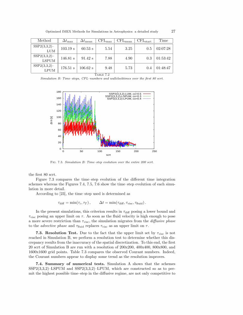
the first 80 scrt.Figure 7.3 compares the time–step evolution of the different time integration
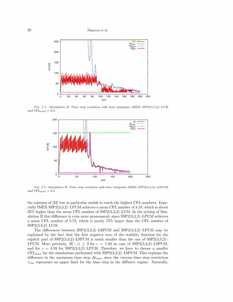
schemes whereas the Figures 7.4, 7.5, 7.6 show the time–step evolution of each simu-lation in more detail.
According to [23], the time–step used is determined as
τdiff = min(τc, τT ) , ∆t = min(τdiff , τvisc, τfluid) .
In the present simulations, this criterion results in τdiff posing a lower bound andτvisc posing an upper limit on τ . As soon as the fluid velocity is high enough to posea more severe restriction than τvisc, the simulation migrates from the diffusive phaseto the advective phase and τfluid replaces τvisc as an upper limit on τ .
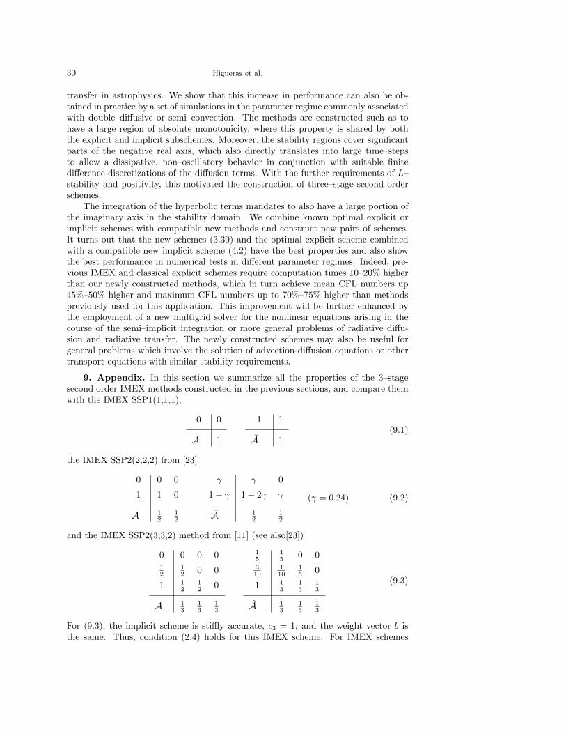
7.3. Resolution Test. Due to the fact that the upper limit set by τvisc is notreached in Simulation B, we perform a resolution test to determine whether this dis-crepancy results from the inaccuracy of the spatial discretization. To this end, the first20 scrt of Simulation B are run with a resolution of 200x200, 400x400, 800x800, and1600x1600 grid points. Table 7.3 compares the observed Courant numbers. Indeed,the Courant numbers appear to display some trend as the resolution improves.
7.4. Summary of numerical tests. Simulation A shows that the schemesSSP2(3,3,2)–LSPUM and SSP2(3,3,2)–LPUM, which are constructed so as to per-mit the highest possible time–step in the diffusive regime, are not only competitive to
28 Higueras et al.
0
50
100
150
200
250
0 20 40 60 80 100 120 140 160 180 200 220
∆t
in [
s]
scrt
∆ t∆tvisc∆tfluid∆tdiff
Fig. 7.4. Simulation B: Time–step evolution with time integrator IMEX SSP2(3,3,2)–LUMand CFLstart = 0.5.
0
50
100
150
200
0 50 100 150 200 250
∆t
in [
s]
scrt
∆t∆tvisc∆tfluid∆tdiff
Fig. 7.5. Simulation B: Time–step evolution with time integrator IMEX SSP2(3,3,2)–LSPUMand CFLstart = 0.3.
the schemes of [23] but in particular enable to reach the highest CFL numbers. Espe-cially IMEX SSP2(3,3,2)–LPUM achieves a mean CFL number of 4.18, which is about35% higher than the mean CFL number of SSP2(3,3,2)–LUM. In the setting of Sim-ulation B this difference is even more pronounced, since SSP2(3,3,2)–LPUM achievesa mean CFL number of 5.73, which is nearly 75% larger than the CFL number ofSSP2(3,3,2)–LUM.
The differences between SSP2(3,3,2)–LSPUM and SSP2(3,3,2)–LPUM may beexplained by the fact that the first negative zero of the stability function for theexplicit part of SSP2(3,3,2)–LSPUM is much smaller than the one of SSP2(3,3,2)–LPUM. More precisely, R(−z) ≥ 0 for z = 1.82 in case of SSP2(3,3,2)–LSPUM,and for z = 3.59 for SSP2(3,3,2)–LPUM. Therefore, we have to choose a smallerCFLstart for the simulations performed with SSP2(3,3,2)–LSPUM. This explains thedifference in the maximum time–step ∆tmax since the viscous time–step restrictionτvisc represents an upper limit for the time–step in the diffusive regime. Naturally,
Optimized IMEX Methods for Simulations in Astrophysics: a detailed study 29
0
50
100
150
200
0 20 40 60 80 100 120 140 160 180 200 220
∆t
in [
s]
scrt
∆ t∆tvisc∆tfluid∆tdiff
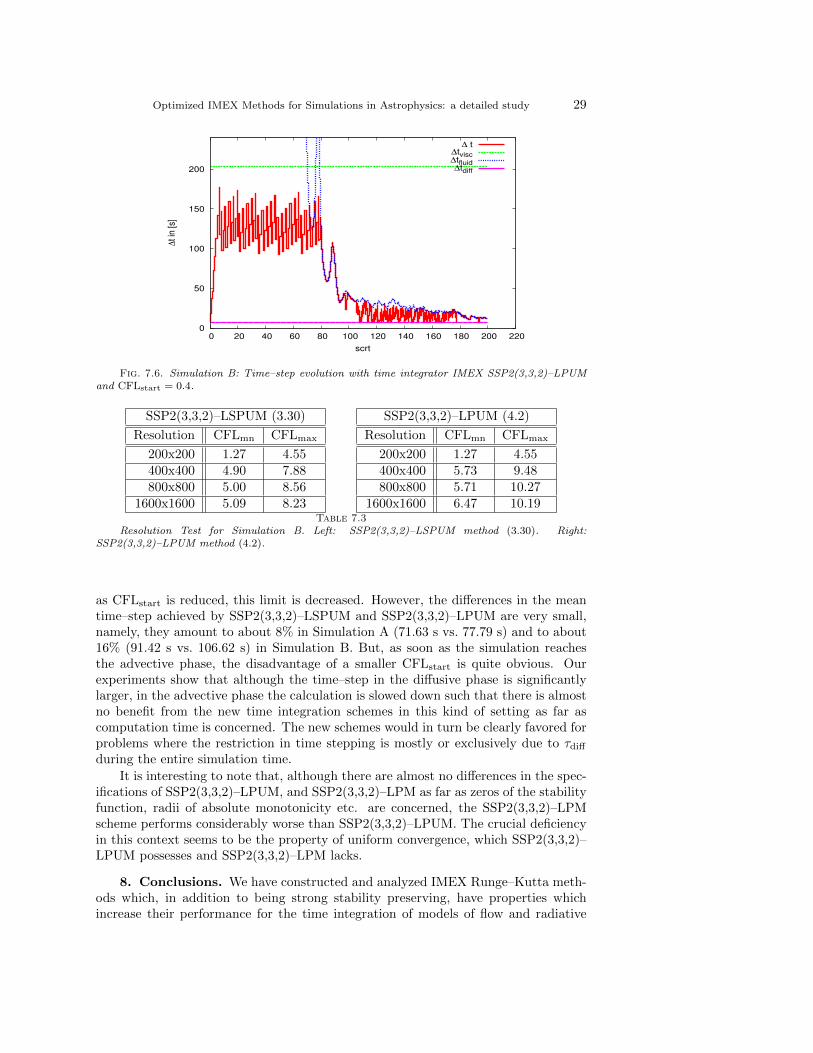
Fig. 7.6. Simulation B: Time–step evolution with time integrator IMEX SSP2(3,3,2)–LPUMand CFLstart = 0.4.
SSP2(3,3,2)–LSPUM (3.30)
Resolution CFLmn CFLmax
200x200 1.27 4.55400x400 4.90 7.88800x800 5.00 8.56
1600x1600 5.09 8.23
SSP2(3,3,2)–LPUM (4.2)
Resolution CFLmn CFLmax
200x200 1.27 4.55400x400 5.73 9.48800x800 5.71 10.27
1600x1600 6.47 10.19Table 7.3
Resolution Test for Simulation B. Left: SSP2(3,3,2)–LSPUM method (3.30). Right:SSP2(3,3,2)–LPUM method (4.2).
as CFLstart is reduced, this limit is decreased. However, the differences in the meantime–step achieved by SSP2(3,3,2)–LSPUM and SSP2(3,3,2)–LPUM are very small,namely, they amount to about 8% in Simulation A (71.63 s vs. 77.79 s) and to about16% (91.42 s vs. 106.62 s) in Simulation B. But, as soon as the simulation reachesthe advective phase, the disadvantage of a smaller CFLstart is quite obvious. Ourexperiments show that although the time–step in the diffusive phase is significantlylarger, in the advective phase the calculation is slowed down such that there is almostno benefit from the new time integration schemes in this kind of setting as far ascomputation time is concerned. The new schemes would in turn be clearly favored forproblems where the restriction in time stepping is mostly or exclusively due to τdiff
during the entire simulation time.
It is interesting to note that, although there are almost no differences in the spec-ifications of SSP2(3,3,2)–LPUM, and SSP2(3,3,2)–LPM as far as zeros of the stabilityfunction, radii of absolute monotonicity etc. are concerned, the SSP2(3,3,2)–LPMscheme performs considerably worse than SSP2(3,3,2)–LPUM. The crucial deficiencyin this context seems to be the property of uniform convergence, which SSP2(3,3,2)–LPUM possesses and SSP2(3,3,2)–LPM lacks.
8. Conclusions. We have constructed and analyzed IMEX Runge–Kutta meth-ods which, in addition to being strong stability preserving, have properties whichincrease their performance for the time integration of models of flow and radiative
30 Higueras et al.
transfer in astrophysics. We show that this increase in performance can also be ob-tained in practice by a set of simulations in the parameter regime commonly associatedwith double–diffusive or semi–convection. The methods are constructed such as tohave a large region of absolute monotonicity, where this property is shared by boththe explicit and implicit subschemes. Moreover, the stability regions cover significantparts of the negative real axis, which also directly translates into large time–stepsto allow a dissipative, non–oscillatory behavior in conjunction with suitable finitedifference discretizations of the diffusion terms. With the further requirements of L–stability and positivity, this motivated the construction of three–stage second orderschemes.
The integration of the hyperbolic terms mandates to also have a large portion ofthe imaginary axis in the stability domain. We combine known optimal explicit orimplicit schemes with compatible new methods and construct new pairs of schemes.It turns out that the new schemes (3.30) and the optimal explicit scheme combinedwith a compatible new implicit scheme (4.2) have the best properties and also showthe best performance in numerical tests in different parameter regimes. Indeed, pre-vious IMEX and classical explicit schemes require computation times 10–20% higherthan our newly constructed methods, which in turn achieve mean CFL numbers up45%–50% higher and maximum CFL numbers up to 70%–75% higher than methodspreviously used for this application. This improvement will be further enhanced bythe employment of a new multigrid solver for the nonlinear equations arising in thecourse of the semi–implicit integration or more general problems of radiative diffu-sion and radiative transfer. The newly constructed schemes may also be useful forgeneral problems which involve the solution of advection-diffusion equations or othertransport equations with similar stability requirements.
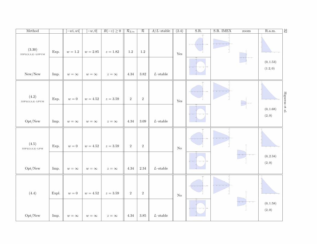
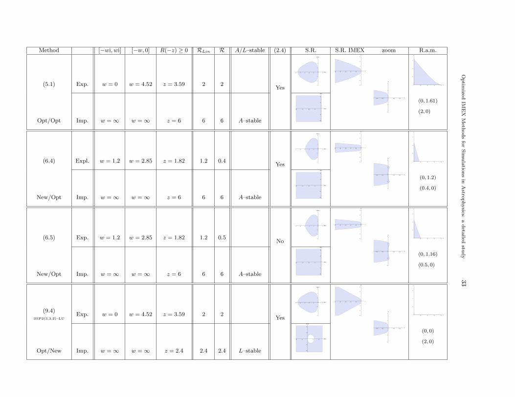
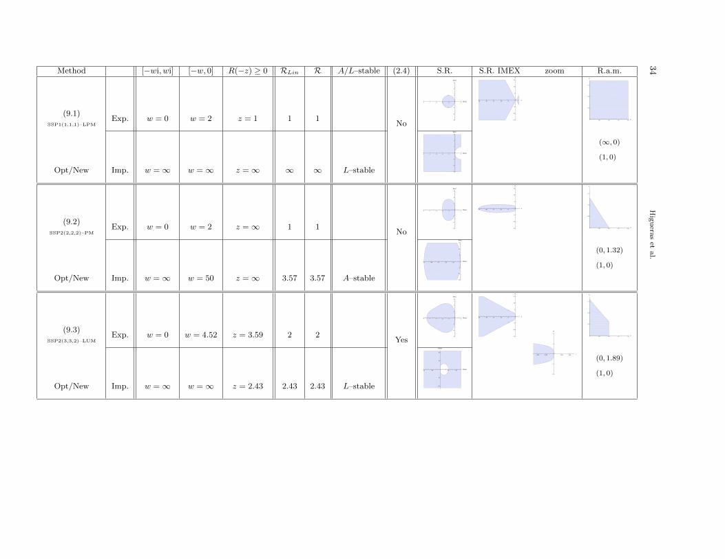
9. Appendix. In this section we summarize all the properties of the 3–stagesecond order IMEX methods constructed in the previous sections, and compare themwith the IMEX SSP1(1,1,1),
0 0
A 1
1 1
A 1(9.1)
the IMEX SSP2(2,2,2) from [23]
0 0 0
1 1 0
A 12
12
γ γ 0
1− γ 1− 2γ γ
A 12
12
(γ = 0.24) (9.2)
and the IMEX SSP2(3,3,2) method from [11] (see also[23])
0 0 0 012
12 0 0
1 12
12 0
A 13
13
13
15
15 0 0
310
110
15 0
1 13
13
13
A 13
13
13
(9.3)
For (9.3), the implicit scheme is stiffly accurate, c3 = 1, and the weight vector b isthe same. Thus, condition (2.4) holds for this IMEX scheme. For IMEX schemes
Optimized IMEX Methods for Simulations in Astrophysics: a detailed study 31
SSP1(1,1,1) and SSP2(2,2,2), condition (2.4) is not satisfied. Due to the knownproperties of the methods, we will refer to (9.1) as SSP1(1,1,1)–LPM, to (9.2) asSSP2(2,2,2)–PM, and to (9.3) as SSP2(3,3,2)–LUM (see (3.33)).
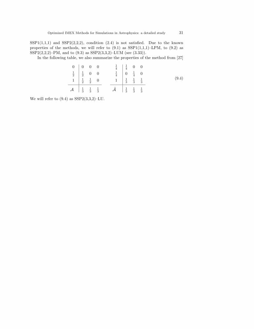
In the following table, we also summarize the properties of the method from [27]
0 0 0 012
12 0 0
1 12
12 0
A 13
13
13
14
14 0 0
14 0 1
4 0
1 13
13
13
A 13
13
13
(9.4)
We will refer to (9.4) as SSP2(3,3,2)–LU.
32
Hig
uera
set
al.
Method [−wi, wi] [−w, 0] R(−z) ≥ 0 RLin R A/L–stable (2.4) S.R. S.R. IMEX zoom R.a.m.
(3.30)SSP2(3,3,2)–LSPUM
Exp. w = 1.2 w = 2.85 z = 1.82 1.2 1.2Yes
-5 -4 -3 -2 -1 1ReHzL
-3
-2
-1
1
2
3
ImHzL
-50 -40 -30 -20 -10z
-15
-10
-5
5
10
15
w
-0.04 -0.02 0.02 0.04z
-2
-1
1
2
w
0.5 1.0 1.5 2.0r1
0.5
1.0
1.5
r2
New/New Imp. w =∞ w =∞ z =∞ 4.34 3.82 L–stable
-20 -10 10 20ReHzL
-20
-10
10
20
ImHzL
(0, 1.53)
(1.2, 0)
(4.2)SSP2(3,3,2)–LPUM
Exp. w = 0 w = 4.52 z = 3.59 2 2Yes
-5 -4 -3 -2 -1 1ReHzL
-3
-2
-1
1
2
3
ImHzL
-50 -40 -30 -20 -10z
-15
-10
-5
5
10
15
w
-0.04 -0.02 0.02 0.04z
-2
-1
1
2
w
0.5 1.0 1.5 2.0r1
0.5
1.0
1.5
r2
Opt/New Imp. w =∞ w =∞ z =∞ 4.34 3.09 L–stable
-20 -10 10 20ReHzL
-20
-10
10
20
ImHzL
(0, 1.68)
(2, 0)
(4.5)SSP2(3,3,2)–LPM
Exp. w = 0 w = 4.52 z = 3.59 2 2No
-5 -4 -3 -2 -1 1ReHzL
-3
-2
-1
1
2
3
ImHzL
-50 -40 -30 -20 -10z
-15
-10
-5
5
10
15
w
-0.04 -0.02 0.02 0.04z
-2
-1
1
2
w
0.5 1.0 1.5 2.0r1
0.5
1.0
1.5
2.0
2.5
r2
Opt/New Imp. w =∞ w =∞ z =∞ 4.34 2.34 L–stable
-20 -10 10 20ReHzL
-20
-10
10
20
ImHzL
(0, 2.34)
(2, 0)
(4.4) Expl. w = 0 w = 4.52 z = 3.59 2 2No
-5 -4 -3 -2 -1 1ReHzL
-3
-2
-1
1
2
3
ImHzL
-50 -40 -30 -20 -10z
-15
-10
-5
5
10
15
w
-0.04 -0.02 0.02 0.04z
-2
-1
1
2
w
0.5 1.0 1.5 2.0r1
0.5
1.0
1.5
r2
Opt/New Imp. w =∞ w =∞ z =∞ 4.34 3.85 L–stable
-20 -10 10 20ReHzL
-20
-10
10
20
ImHzL
(0, 1.58)
(2, 0)
Op
timized
IME
XM
ethod
sfo
rS
imu
latio
ns
inA
strop
hysics:
ad
etailed
stud
y33
Method [−wi, wi] [−w, 0] R(−z) ≥ 0 RLin R A/L–stable (2.4) S.R. S.R. IMEX zoom R.a.m.
(5.1) Exp. w = 0 w = 4.52 z = 3.59 2 2Yes
-5 -4 -3 -2 -1 1ReHzL
-3
-2
-1
1
2
3
ImHzL
-50 -40 -30 -20 -10z
-15
-10
-5
5
10
15
w
-0.04 -0.02 0.02 0.04z
-2
-1
1
2
w
0.5 1.0 1.5 2.0r1
0.5
1.0
1.5
r2
Opt/Opt Imp. w =∞ w =∞ z = 6 6 6 A–stable
-20 -15 -10 -5ReHzL
-20
-10
10
20
ImHzL
(0, 1.61)
(2, 0)
(6.4) Expl. w = 1.2 w = 2.85 z = 1.82 1.2 0.4Yes
-5 -4 -3 -2 -1 1ReHzL
-3
-2
-1
1
2
3
ImHzL
-50 -40 -30 -20 -10z
-15
-10
-5
5
10
15
w
-0.04 -0.02 0.02 0.04z
-2
-1
1
2
w
0.5 1.0 1.5 2.0r1
0.5
1.0
1.5
r2
New/Opt Imp. w =∞ w =∞ z = 6 6 6 A–stable
-20 -15 -10 -5ReHzL
-20
-10
10
20
ImHzL
(0, 1.2)
(0.4, 0)
(6.5) Exp. w = 1.2 w = 2.85 z = 1.82 1.2 0.5No
-5 -4 -3 -2 -1 1ReHzL
-3
-2
-1
1
2
3
ImHzL
-50 -40 -30 -20 -10z
-15
-10
-5
5
10
15
w
-0.04 -0.02 0.02 0.04z
-2
-1
1
2
w
0.5 1.0 1.5 2.0r1
0.5
1.0
1.5
r2
New/Opt Imp. w =∞ w =∞ z = 6 6 6 A–stable
-20 -15 -10 -5ReHzL
-20
-10
10
20
ImHzL
(0, 1.16)
(0.5, 0)
(9.4)SSP2(3,3,2)–LU
Exp. w = 0 w = 4.52 z = 3.59 2 2Yes
-5 -4 -3 -2 -1 1ReHzL
-3
-2
-1
1
2
3
ImHzL
-50 -40 -30 -20 -10z
-15
-10
-5
5
10
15
w
-0.04 -0.02 0.02 0.04z
-2
-1
1
2
w
0.5 1.0 1.5 2.0r1
0.5
1.0
1.5
r2
Opt/New Imp. w =∞ w =∞ z = 2.4 2.4 2.4 L–stable
-20 -10 10 20ReHzL
-20
-10
10
20
ImHzL
(0, 0)
(2, 0)
34
Hig
uera
set
al.
Method [−wi, wi] [−w, 0] R(−z) ≥ 0 RLin R A/L–stable (2.4) S.R. S.R. IMEX zoom R.a.m.
(9.1)SSP1(1,1,1)–LPM
Exp. w = 0 w = 2 z = 1 1 1No
-5 -4 -3 -2 -1 1ReHzL
-3
-2
-1
1
2
3
ImHzL
-50 -40 -30 -20 -10z
-15
-10
-5
5
10
15
w
0.5 1.0 1.5 2.0r1
0.5
1.0
1.5
r2
Opt/New Imp. w =∞ w =∞ z =∞ ∞ ∞ L–stable
-5 -4 -3 -2 -1 1ReHzL
-3
-2
-1
1
2
3
ImHzL
(∞, 0)
(1, 0)
(9.2)SSP2(2,2,2)–PM
Exp. w = 0 w = 2 z =∞ 1 1No
-5 -4 -3 -2 -1 1ReHzL
-3
-2
-1
1
2
3
ImHzL
-50 -40 -30 -20 -10z
-15
-10
-5
5
10
15
w
0.5 1.0 1.5 2.0r1
0.5
1.0
1.5
r2
Opt/New Imp. w =∞ w = 50 z =∞ 3.57 3.57 A–stable
-50 -40 -30 -20 -10ReHzL
-15
-10
-5
5
10
15
ImHzL
(0, 1.32)
(1, 0)
(9.3)SSP2(3,3,2)–LUM
Exp. w = 0 w = 4.52 z = 3.59 2 2Yes
-5 -4 -3 -2 -1 1ReHzL
-3
-2
-1
1
2
3
ImHzL
-50 -40 -30 -20 -10z
-15
-10
-5
5
10
15
w
-0.04 -0.02 0.02 0.04z
-2
-1
1
2
w
0.5 1.0 1.5 2.0r1
0.5
1.0
1.5
r2
Opt/New Imp. w =∞ w =∞ z = 2.43 2.43 2.43 L–stable
-20 -10 10 20ReHzL
-20
-10
10
20
ImHzL
(0, 1.89)
(1, 0)
Optimized IMEX Methods for Simulations in Astrophysics: a detailed study 35
REFERENCES
[1] S. Boscarino, Error analysis of IMEX Runge–Kutta methods derived from differential–algebraic systems, SIAM J. Numer. Anal., 45 (2008), pp. 1600–1621.
[2] M.P. Calvo, J. De Frutos, and J. Novo, Linearly implicit Runge–Kutta methods foradvection-reaction-diffusion equations, Appl. Numer. Math., 37 (2001), pp. 535–549.
[3] L. Ferracina and M. Spijker, An extension and analysis of the Shu–Osher representation ofRunge–Kutta methods, Math. Comp., 74 (2004), pp. 201–219.
[4] , Strong stability of singly-diagonally-implicit Runge–Kutta methods, Appl. Numer.Math., 58 (2008), pp. 1675–1686.
[5] S. Gottlieb, D. Ketcheson, and C.-W. Shu, High order strong stability preserving timediscretizations, J. Sci. Comput., 38 (2009), pp. 251–289.
[6] S. Gottlieb and C.-W. Shu, Total variation diminishing Runge–Kutta schemes, Math.Comp., 67 (1998), pp. 73–85.
[7] S. Gottlieb, C.-W. Shu, and E. Tadmor, Strong stability-preserving high-order time dis-cretization methods, SIAM Rev., 43 (2001), pp. 89–112.
[8] E. Hairer and G. Wanner, Solving Ordinary Differential Equations II, Springer-Verlag,Berlin–Heidelberg–New York, 1991.
[9] I. Higueras, On strong stability preserving time discretization methods, J. Sci. Comput., 21(2004), pp. 193–223.
[10] , Representations of Runge–Kutta methods and strong stability preserving methods,SIAM J. Numer. Anal., 43 (2005), pp. 924–948.
[11] , Strong stability for additive Runge–Kutta methods, SIAM J. Numer. Anal., 44 (2006),pp. 1735–1758.
[12] , Characterizing strong stability preserving additive Runge–Kutta methods, J. Sci. Com-put., 39 (2009), pp. 115–128.
[13] W. Hundsdorfer, A. Mozartova, and M. Spijker, Stepsize restrictions for boundednessand monotonicity in numerical initial value problems, SIAM J. Numer. Anal., 47 (2009),pp. 3797–3819.
[14] W. Hundsdorfer and M. Spijker, Boundedness and strong stability of Runge–Kutta methods,Math. Comp., 80 (2011), pp. 863–886.
[15] W. Hundsdorfer and J. G. Verwer, Numerical Solution of Time-Dependent Advection-Diffusion-Reaction Equations, Springer, 2003.
[16] A. Iserles, A first course in the numerical analysis of differential equations, Cambridge Uni-versity Press, 1996.
[17] D. Ketcheson, Highly efficient strong stability preserving Runge–Kutta methods with lowstorage implementations, SIAM J. Sci. Comput., 30 (2008), pp. 2113–2136.
[18] D. Ketcheson, C.B. MacDonald, and S. Gottlieb, Optimal implicit strong stability pre-serving Runge–Kutta methods, Appl. Numer. Math., 59 (2009), pp. 373–392.
[19] D. Ketcheson, C. Macdonald, and S. Gottlieb, Optimal implicit strong stability preservingRunge–Kutta methods, Appl. Numer. Math., 59 (2009), pp. 373–392.
[20] O. Koch, F. Kupka, B. Low-Baselli, A. Mayrhofer, and F. Zaussinger,SDIRK methods for the ANTARES code, ASC Report 32/2010, Inst. forAnal. and Sci. Comput., Vienna Univ. of Technology, 2010. Available athttp://www.asc.tuwien.ac.at/preprint/2010/asc32x2010.pdf.
[21] J.F.B.M. Kraaijevanger, Contractivity of Runge–Kutta methods, BIT, 31 (1991), pp. 482–528.
[22] J. F. B. M. Kraaijevanger, Absolute monotonicity of polynomials occurring in the numericalsolution of initial value problems, Numer. Math., 48 (1986), pp. 303–322.
[23] F. Kupka, N. Happenhofer, I. Higueras, and O. Koch, Total–variation–diminishingimplicit–explicit Runge–Kutta methods for the simulation of double-diffusive convectionin astrophysics, J. Comput. Phys., 231 (2012), pp. 3561–3586.
[24] M. Motamed, C.B. Macdonald, and S.J. Ruuth, On the linear stability of the fifth-orderWENO discretization, J. Sci. Comput., 47 (2011), pp. 127–149.
[25] H.J. Muthsam, F. Kupka, B. Low-Baselli, C. Obertscheider, M. Langer, and P. Lenz,ANTARES — A Numerical Tool for Astrophysical RESearch with applications to solargranulation, New Astronomy, 15 (2010), pp. 460–475.
[26] L. Pareschi and G. Russo, Implicit-explicit Runge-Kutta schemes for stiff systems of differ-ential equations, Recent trends in numerical analysis, 3 (2000), pp. 269–289.
[27] , Implicit–explicit Runge–Kutta schemes and application to hyperbolic systems with re-laxation, J. Sci. Comput., 25 (2005), pp. 129–155.
[28] C.-W. Shu, Total-variation-diminishing time discretizations, SIAM J. Sci. Statist. Comput., 9
36 Higueras et al.
(1988), pp. 1073–1084.[29] , A survey of strong stability-preserving high-order time discretization methods, in Col-
lected Lectures on the Preservation of Stability under Discretization, SIAM, Philadelphia,PA, 2002, pp. 51–65.
[30] C.-W. Shu and S. Osher, Efficient implementation of essentially non-oscillatory shock–capturing schemes, J. Comput. Phys., 77 (1988), pp. 439–471.
[31] M. Spijker, Contractivity in the numerical solution of initial value problems, Numer. Math.,42 (1983), pp. 271–290.
[32] M.N. Spijker, Stepsize restrictions for stability of one-step methods in the numerical solutionof initial value problems, Math. Comp., 45 (1985), pp. 377–392.
[33] M. Spijker, Stepsize conditions for general monotonicity in numerical initial value problems,SIAM J. Numer. Anal., 45 (2007), pp. 1226–1245.
[34] J.C. Strikwerda, Finite Difference Schemes and Partial Differential Equations, SIAM,Philadelphia, PA, 2nd ed., 2004.
[35] J.A. Van de Griend and J. J. Kraaijevanger, Absolute monotonicity of rational functionsoccurring in the numerical solution of initial value problems, Numer. Math., 49 (1986),pp. 413–424.
[36] R. Wang and R.J. Spiteri, Linear instability of the fifth-order WENO method, SIAM J.Numer. Anal., 45 (2007), pp. 1871–1901.