Embed Size (px)
Citation preview
Topical Report Optimized Reservoir History Matching Simulation of Canyon Formation, SACROC Unit, Permian Basin Performed by: Karine Schepers, Reinaldo J. González, and Scott R. Reeves Advanced Resources International, Inc. 11490 Westheimer Rd., Suite 520 Houston, TX 77077 November 9, 2007 Prepared for: U.S. Department of Energy Contract No. DE-FC26-04NT15514
SACROC Simulation KS080807
i
Disclaimers
U.S. Department of Energy This report was prepared as an account of work sponsored by an agency of the United States Government. Neither the United States Government nor any agency thereof, nor any of their employees, makes any warranty, express or implied, or assumes any legal liability or responsibility for the accuracy, completeness, or usefulness of any information, apparatus, product, or process disclosed, or represents that its use would not infringe privately owned rights. Reference herein to any specific commercial product, process, or service by trade name, trademark, manufacturer, or otherwise does not necessarily constitute or imply its endorsement, recommendation, or favoring by the United States Government or any agency thereof. The views and opinions of authors expressed herein do not necessarily state or reflect those of the United States Government or any agency thereof.
Advanced Resources International, Inc.
The material in this Report is intended for general information only. Any use of this material in relation to any specific application should be based on independent examination and verification of its unrestricted applicability for such use and on a determination of suitability for the application by professionally qualified personnel. No license under any Advanced Resources International, Inc., patents or other proprietary interest is implied by the publication of this Report. Those making use of or relying upon the material assume all risks and liability arising from such use or reliance.
SACROC Simulation KS080807
ii
Executive Summary
Accurate, high-resolution, three-dimensional (3D) reservoir characterization can provide substantial benefits for effective oilfield management. By doing so, the predictive reliability of reservoir flow models, which are routinely used as the basis for significant investment decisions designed to recover millions of barrels of oil, can be substantially improved. This is particularly true when Secondary Oil Recovery (SOR) or Enhanced Oil Recovery (EOR) operations are planned. If injectants such as water, hydrocarbon gasses, steam, CO2, etc. are to be used; an understanding of fluid migration paths can mean the difference between economic success and failure. SOR/EOR projects will increasingly take place in heterogeneous reservoirs where interwell complexity is high and difficult to understand. The industry therefore needs improved reservoir characterization approaches that are quicker, more accurate, and less expensive than today’s standard methods.
To achieve this objective, the Department of Energy (DOE) has been promoting some
studies with the goal of evaluating whether robust relationships between data at vastly different scales of measurement could be established using advanced pattern recognition (soft computing) methods. Advanced Resources International (ARI) has performed two of these projects with encouraging results showing the feasibility of establishing critical relationships between data at different measurement scales to create high-resolution reservoir characterization.
In this third study performed by ARI and also funded by the DOE, a model-based,
probabilistic clustering analysis procedure is successfully applied to generate a high-resolution reservoir characterization outcome. The approach was applied in the Pennsylvanian-Permian reef carbonates (Cisco and Canyon Formations) of a subregion of the SACROC Unit, Horseshoe Atoll, Permian Basin, Texas, and acknowledged as a highly complex carbonate reservoir.
A selected area within the SACROC Unit platform was used for this study. In the first stage
of this project, a two-step “soft-computing” procedure was developed for efficiently generating core-scale porosity and permeability values (as well as rock types geologically consistent) at well locations where only gamma ray (GR) and neutron porosity logs (NPHI) were available. In this way, “core” parameter profiles, with high vertical resolution, could be generated for many wells which permitted to populate any well location with core-scale estimates of porosity and permeability (P&P) and rock types facilitating direct application of geostatistical methods to build 3D reservoir models. This process provided a data set considered sufficient to characterize directly the reservoir representations of P&P. Next, in the second stage of the project, stochastic simulation algorithms were utilized to construct high resolution characterizations of P&P in the selected study region.
The models developed in this study successfully captured the nature of lithofacies
distributions and depositional environments, providing genuine representations of P&P in concordance with the selected grid resolution for characterizing the studied region. In the final stage of this project, validation of the porosity and permeability representations was done by a computer-assisted reservoir simulation history-match of prior production, which was achieved without
SACROC Simulation KS080807
iii
significant changes to the original characterization of the studied region. For these purposes, a black-oil model was utilized, and this report focuses on the reservoir modeling and history matching of 57 years of production data for 19 producing wells included in the study area. As a consequence, the validation result of the reservoir characterization methodology is presented.
An assisted history match was achieved using a global optimization method (evolutionary
algorithms). This history match, in which several results were produced, was based on the matching of oil, gas and water production rates, and the average reservoir pressure. The match was accomplished by manipulating 13 uncertain design parameters which included two formation properties, other ten variables related with the corresponding relative permeability curves, and one variable linked to the reservoir production. Evolutionary algorithms can handle a large amount of input design parameters. And, in this work, they were successfully applied for history matching complex reservoir performance drivers thanks to their capabilities to explore an enormous range of parameter combinations and produce lots of results related to the reservoir performance.
History match results confirmed that the 3D reservoir models of P&P constructed applying
the combined reservoir characterization approach (advanced pattern recognition techniques and geostatistical algorithms) were legitimate representations of the spatial distribution of these parameters. In addition, they confirmed initial assumptions that the developed porosity model was highly trustworthy, whereas the permeability model, despite of capturing correctly geological trends and heterogeneities of Canyon Reef reservoir (SACROC field) presented slightly underestimated values.
The modeling efforts resulted in a very good history match for the center wells in the study
area. A good match was also achieved for the outer producing wells and the average reservoir pressure. These achievements were thanks to the setting up of proper boundary conditions that described the flow behavior at the boundary of the analyzed region. Overall, the match of liquid production rate was very well achieved. Matches of oil, gas and water production rates were from satisfactory to very good. The average reservoir pressure match was also of good quality although slightly high between years 1972 and 1988.
The simple black oil model developed here was sufficient to capture the reservoir behavior
of SACROC Unit, Canyon Reef Formation since simulated oil-water relative permeability curves match perfectly actual core measurement, and a recovery factor equal to 46% (a maximum of 39% was reported in literature) was obtained from the simulated reservoir model. This factor was probably overestimated due to the injection of miscible gas in our black-oil model, when immiscibility injection should have occurred.
The addition of optimization methods (for assisted history matching) to the combined soft-
computing/geostatistical approach (utilized for reservoir characterization purposes) constituted a powerful triad of mathematical techniques ideally suited for addressing reservoir integrated studies, with the capacity of facing these complex tasks more rapidly and efficiently than using traditional methodologies.
SACROC Simulation KS080807
iv
Table of Contents Disclaimers...........................................................................................................................................i
Executive Summary ...........................................................................................................................ii
List of Tables.......................................................................................................................................v
List of Figures ....................................................................................................................................vi
1.0 Introduction ............................................................................................................................1
3.0 Methodology ...........................................................................................................................4
4.0 Field and Reservoir Description and Development ............................................................5
4.1 Field Description..................................................................................................................5
4.2 Reservoir Description: Petrophysical Data .......................................................................11
4.3 Reservoir Description: Fluid Data ....................................................................................15
4.4 Production Data.................................................................................................................18
5.0 Reservoir Simulation............................................................................................................21
5.1 Reservoir Model Construction ...........................................................................................21
5.2 Model Boundary Conditions ..............................................................................................29
6.0 History Matching..................................................................................................................40
6.1 Procedure ...........................................................................................................................40
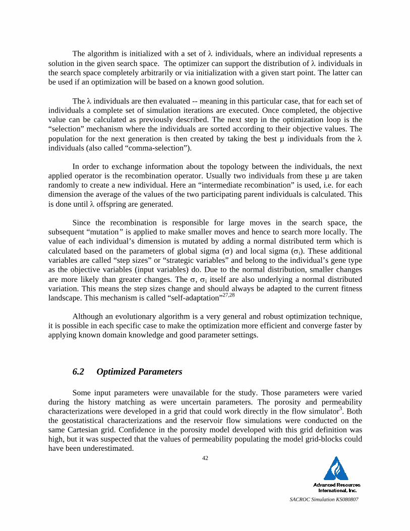
6.2 Optimized Parameters........................................................................................................42
6.3 Results ................................................................................................................................44
7.0 Conclusions ...........................................................................................................................59
8.0 References .............................................................................................................................61
Appendix A: History Matching Results – Outer Wells ..............................................................A-1
SACROC Simulation KS080807
v
List of Tables Table 1: Available Formation Properties..........................................................................................................15 Table 2: Available Fluid Properties..................................................................................................................15 Table 3: Available PVT Data ...........................................................................................................................15 Table 4: Formation, Fluid and Well Properties of the Reservoir Model ..........................................................24 Table 5: Material Balance Symbols25 ...............................................................................................................37 Table 6: Fixed Parameters During History Matching.......................................................................................43 Table 7: Varying parameters during History Matching....................................................................................44 Table 8: Optimized Parameters Obtained for the Match ..................................................................................54
SACROC Simulation KS080807
vi
List of Figures Figure 1: Location of Kelly Snyder Field, SACROC Unit2.......................................................................... 5 Figure 2: Location of Study Area, Kelly Snyder Field2................................................................................ 6 Figure 3: Stratigraphic Column and Type-Log of Permian Basin, SACROC Unit6, 7 .................................. 7 Figure 4: Canyon Reef Formation – Cross Section2 ..................................................................................... 7 Figure 5: Kelly-Snyder Field Performance History6..................................................................................... 9 Figure 6: Kelly Snyder Field Reservoir Pressure 1948-19725 ...................................................................... 9 Figure 7: Bottom-Hole Pressure Maps, SACROC Unit Area, Kelly-Snyder Field5................................... 10 Figure 8: SACROC Unit, 1992 Pressure Contour Map7............................................................................. 11 Figure 9: Four Different Geostatistical Realizations of Porosity3............................................................... 12 Figure 10: Geostatistical Characterization of Porosity3 used in the Reservoir Simulation......................... 13 Figure 11: Histogram of Porosity Characterization Values3 used in the Reservoir Simulation.................. 13 Figure 12: Geostatistical Characterization of Permeability3 used in the Reservoir Simulation.................. 14 Figure 13: Histogram of the Permeability Characterization Values3 used in the Reservoir Simulation..... 14 Figure 14: Oil-Water Relative Permeability Curves, Well 32-3................................................................. 16 Figure 15: Oil-Water Relative Permeability Curves, Well 34-6................................................................. 16 Figure 16: Available Capillary Pressure Curves......................................................................................... 17 Figure 17: Producing and Injecting Wells Included in the Study Area2, 3................................................... 18 Figure 18: Production Rates for the Modeled Study Area.......................................................................... 19 Figure 19: Injection Rates for the Modeled Study Area ............................................................................. 19 Figure 20: Porosity Model of the Study Area ............................................................................................. 22 Figure 21: Horizontal Permeability Model of the Study Area.................................................................... 23 Figure 22: Oil Formation Volume Factor vs. Pressure ............................................................................... 24 Figure 23: Oil Viscosity vs. Pressure.......................................................................................................... 25 Figure 24: Gas Oil Ratio vs. Pressure ......................................................................................................... 25 Figure 25: Inverted Gas Formation Volume Factor vs. Pressure................................................................ 26 Figure 26: Gas Viscosity vs. Pressure......................................................................................................... 26 Figure 27: Oil-Water Capillary Pressure Curve vs. Real Data ................................................................... 27 Figure 28: Study Area Reservoir Model - Top View.................................................................................. 28 Figure 29: Study Area Reservoir Model - 3D View ................................................................................... 29
SACROC Simulation KS080807
vii
Figure 30: Top View of the SACROC Platform Model ............................................................................. 30 Figure 31: 2D View of the SACROC Platform Model (IK Plan) ............................................................... 30 Figure 32: 3D View of the SACROC Platform Model ............................................................................... 31 Figure 33: Flux at the North Edge of the Study Area ................................................................................. 32 Figure 34: Flux at the South Edge of the Study Area ................................................................................. 32 Figure 35: Flux at the West Edge of the Study Area .................................................................................. 33 Figure 36: Flux at the East Edge of the Study Area.................................................................................... 33 Figure 37: Total Fluxes at Edges of the Study Area ................................................................................... 34 Figure 38: Differential Water Volume for the Model (Water Production - Water Injection)..................... 35 Figure 39: Comparison of Total Water Fluxes Computed from Method 1 and Method 2.......................... 36 Figure 40: Location of the 12 Pseudo-Injectors (in Red) Inside the Four Quadrants of the Study Area .... 38 Figure 41: Water Flux per Quadrant (from Method 2) ............................................................................... 39 Figure 42: Optimization Process Workflow ............................................................................................... 41 Figure 43: History Match of Gas Rate, Well P-33-1 .................................................................................. 45 Figure 44: History Match of Oil and Water Rates, Well P-33-1 ................................................................ 45 Figure 45: History Match of Gas Rate, Well P-33-15 ................................................................................ 46 Figure 46: History Match of Oil and Water Rates, Well P-33-15 .............................................................. 46 Figure 47: History Match of Gas Rate, Well P-36-C3................................................................................ 47 Figure 48: History Match of Oil and Water Rates, Well P-36-C3.............................................................. 47 Figure 49: History Match of Gas Rate, Well P-37-4 .................................................................................. 48 Figure 50: History Match of Oil and Water Rates, Well P-37-4 ................................................................ 48 Figure 51: History Match of Gas Rate, Well P-37-5 .................................................................................. 49 Figure 52: History Match of Oil and Water Rates, Well P-37-5 ................................................................ 49 Figure 53: History Match of Gas Rate, Well P-37-6 .................................................................................. 50 Figure 54: History Match of Oil and Water Rates, Well P-37-6 ................................................................ 50 Figure 55: History Match of Gas Rate, Well P-59-1 .................................................................................. 51 Figure 56: History Match of Oil and Water Rates, Well P-59-1 ................................................................ 51 Figure 57: History Match of Gas Rate, Well P-62-1 .................................................................................. 52 Figure 58: History Match of Oil and Water Rates, Well P-62-1 ................................................................ 52 Figure 59: History Match of Average Reservoir Pressure .......................................................................... 53 Figure 60: Optimized Oil-Water Relative Permeability Curves ................................................................. 55 Figure 61: Optimized Gas-Liquid Relative Permeability Curves ............................................................... 55
SACROC Simulation KS080807
viii
Figure 62: Total Error Function vs. Number of Runs................................................................................. 56 Figure 63: Convergence of the Permeability Multiplier ............................................................................. 56 Figure 64: Irreducible Water Saturation Convergence ............................................................................... 57 Figure 65: 3D View of Residual Oil Saturation at the End of the Simulation............................................ 58 Figure A-1: History Match of Gas Rate, Well P-33-2 ..............................................................................A-1 Figure A-2: History Match of Oil and Water Rates, Well P-33-2 ............................................................A-1 Figure A-3: History Match of Gas Rate, Well P-33-11 ............................................................................A-2 Figure A-4: History Match of Oil and Water Rates, Well P-33-11 ..........................................................A-2 Figure A-5: History Match of Gas Rate, Well P-33-14 ............................................................................A-3 Figure A-6: History Match of Oil and Water Rates, Well P-33-14 ..........................................................A-3 Figure A-7: History Match of Gas Rate, Well P-36-5 ..............................................................................A-4 Figure A-8: History Match of Oil and Water Rates, Well P-36-5 ............................................................A-4 Figure A-9: History Match of Gas Rate, Well P-36-7 ..............................................................................A-5 Figure A-10: History Match of Oil and Water Rates, Well P-36-7 ..........................................................A-5 Figure A-11: History Match of Gas Rate, Well P-36-8 ............................................................................A-6 Figure A-12: History Match of Oil and Water Rates, Well P-36-8 ..........................................................A-6 Figure A-13: History Match of Gas Rate, Well P-37-8 ............................................................................A-7 Figure A-14: History Match of Oil and Water Rates, Well P-37-8 ..........................................................A-7 Figure A-15: History Match of Gas Rate, Well P-58-1 ............................................................................A-8 Figure A-16: History Match of Oil and Water Rates, Well P-58-1 ..........................................................A-8
SACROC Simulation KS080807
1
1.0 Introduction Accurate, high-resolution, three-dimensional (3D) reservoir characterization can provide
substantial benefits for effective oilfield management. Even a small improvement in incremental oil recovery for high-value assets can result in important contributions to bottom-line profitability.
This is particularly true when Secondary Oil Recovery (SOR) or Enhanced Oil Recovery
(EOR) operations are planned. If water, hydrocarbon gasses, steam or CO2 are to be used, an understanding of fluid migration paths can mean the difference between economic success or failure. In these types of projects, injectant costs can be a significant part of operating expenses, and hence their optimized utility is critical.
Although reasonable reservoir characterization information often exists at the wellbore,
the only economical way to sample the interwell region is with seismic methods. Surface reflection seismic has relatively low cost per unit volume of reservoir investigated, but the resolution of surface seismic data available today, particularly in the vertical dimension, is not sufficient to produce the kind of detailed reservoir description necessary for effective SOR/EOR optimization and planning.
Today’s standard practice for developing a 3D reservoir description is to use seismic
inversion techniques. These techniques make use of rock physics concepts to solve the inverse problem, i.e., to iteratively construct a likely geologic model and then upscale and compare its acoustic response to that actually observed in the field. This method suffers from the fact that rock physics relationships are not well understood, and the need to rely on porosity-permeability transforms to estimate permeability from porosity. Further, these methods require considerable resources to perform, and thus it is applied to only a small percentage of oil and gas producing assets.
Since the majority of fields do not utilize these technologies currently, many fields are
sub-optimally developed. The industry therefore needs an improved reservoir characterization approach that is quicker, more accurate, and less expensive than today’s standard methods. This will permit more reservoirs to be better characterized, allowing recoveries to be optimized and significantly adding to recoverable reserves.
A new approach to achieve this objective was first examined in a Department of Energy
(DOE) study performed by Advanced Resources International (ARI) in 2000/20011. The goal of that study was to evaluate whether robust relationships between data at vastly different scales of measurement could be established using virtual intelligence (VI) methods. The proposed workflow required that three specific relationships be established through use of data-driven modeling methods, in that case Artificial Neural Networks (ANN’s): core-to-log, log-to-
SACROC Simulation KS080807
2
crosswell seismic and crosswell-to-surface seismic. A key attribute of this approach is the inclusion of borehole seismic (such as crosswell and/or vertical seismic profiling – VSP) in the data collection scheme. Borehole seismic fills a critical gap in the resolution spectrum of reservoir measurements between the well log and surface seismic scales, thus establishing important constraints on characterization outcomes.
The results of the initial study showed that it is, in fact, feasible to establish the three
critical relationships required, and that use of data at different scales of measurement to create high-resolution reservoir characterization is possible. The study showed sufficient promise in the utility of soft-computing methods for reservoir characterization that further refinement of the process was undertaken.
In this study, performed by ARI and funded by the DOE, the same approach was again
utilized to generate a high-resolution reservoir characterization outcome as a first stage in an integrated clustering/geostatistical approach for 3D reservoir characterization. The entire study, subject of previous reports2,3, was performed at the SACROC Unit, operated by Kinder Morgan CO2 Co., L.P (KMCO2), in the Permian basin of West Texas.
The SACROC Unit was formed in 1952 to facilitate coordinated water flooding operations in the field, which began in 1954. CO2-EOR began in 1972 originally using anthropogenic CO2, and in recent years has primarily been focused in the Central Plain area of the unit where reservoir architecture is more horizontal and therefore amenable to pattern flooding.
The decade of the 1990’s found operations at a critical juncture in the field. Production
had been dropping more than 20% per year from a peak of 210,000 barrels of oil per day (BOPD) in the mid-1970’s to only 9,000 BOPD in 1995. The field was considered to be very mature by the mid-1990s, and the estimated economic limit was rapidly approaching. The Unit owners were faced with a significant abandonment effort including negative cash flow and abandonment liability. However, under the leadership of a new operator (Pennzoil), a long-term plan was implemented to arrest the production decline, reduce expenditures, and ultimately restore the economic viability of the Unit.
Since acquiring SACROC in 2000, KMCO2 has succeeded in reducing costs and has
almost tripled production via a more focused and aggressive CO2 injection program, as well as better well pattern management. KMCO2 has increased oil production to 23,000 BOPD, and is now considering production operation options for the 1-3 billion barrel (OOIP) Northern Platform portion of the field. The area appears to have the necessary reservoir characteristics for hosting a gravity-stable flood in some regions. However, reservoir pressure may be below the minimum miscibility pressure (MMP) since operations have been nominal since the 1990’s. Therefore, aggressive CO2 injection and pressure control efforts will be needed.
SACROC Simulation KS080807
3
A better understanding of the reservoir properties could make the difference between economic success or failure in future development of the field. Developing legitimate models of the porosity and permeability distributions in a selected study area of SACROC was the goal of this project. The models developed in this study successfully captured the nature of lithofacies distributions and depositional environments, providing genuine representations of permeability and porosity in concordance with the selected grid resolution for characterizing the studied region.
Validation of the representations was done by history matching using porosity and permeability characterizations, production data, and reservoir simulation. A black-oil model was then built.
This report focuses on the reservoir modeling and history matching of 57 years of
production data for 19 producing wells included in the study area. The specific objectives of this study were: - To create a reservoir simulation model using the reservoir characterization generated
in previous stages of the project (see topical reports2, 3). - To match the individual production of each well included in the study area - To match reservoir pressure as well - To be able to understand the fundamentals of the reservoir performance using a
simple black oil reservoir model - To use the model as a base for an eventual more-advanced compositional model,
covering a larger area of the Northern platform.
The methodology employed to achieve the project objective was as follow: - Create a simple black oil model covering the study area and including the
geostatistical porosity and permeability characterizations previously generated - Estimate proper boundary conditions around the model using several different
techniques - Implement pseudo wells to reproduce proper flux at the edge of the model - History match the production history of each individual producing well inside the
study area
This report presents the results of the validation of the reservoir characterization and the history matching of 19 producing wells and the reservoir pressure.
SACROC Simulation KS080807
4
3.0 Methodology
The reservoir model built in this study covers an area selected jointly with the operator KMCO2. The area was chosen based on the existence of a completely cored well (well 37-11), a planned crosswell seismic survey inside the area, and a future CO2 injection procedure to be implemented to improve the production levels. Porosity and permeability distributions were defined using geostatistical characterizations extensively described in previous topical reports2, 3. KMCO2 provided production and injection data, and PVT and formation data came from published literature. A black oil model of more than 65,000 grid-blocks was build which included the 19 producing wells and 3 injecting wells.
The ability to reproduce proper boundary conditions at the edge of the model was critical
to achieve a good match. Boundary conditions at the edge of the models were calculated using several different methods (simple large scale reservoir model, differential water volume calculations, and material balance). Pseudo wells were incorporated at the edge of the modeled area to reproduce water fluxes. However, some uncertainties remained because the different methods gave different answers. Therefore, a factor controlling water fluxes at the edge of the model was used, and was optimized during the history matching process.
For each individual producing well included in the study area, liquid, water and gas
production rates were history matched. We were confident in the upscaling of porosity; hence, original porosity realization was used as-is in the reservoir model. However, it was anticipated that upscaled permeability would probably underestimate actual permeability. To preserve geological trends and heterogeneities, the original permeability characterization was used but was multiplied by a factor between 1 and 5 that needed to be optimized during the history matching process.
The final objective was to understand and to reproduce the reservoir performance of
Canyon Reef formation in the Kelly-Snyder field using a simple but accurate black-oil model. The history matching would be achieved by using an automated optimization process.
SACROC Simulation KS080807
5
4.0 Field and Reservoir Description and Development
4.1 Field Description
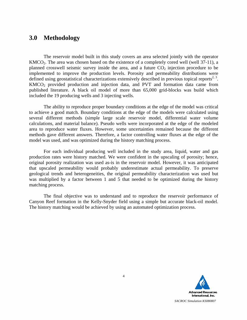
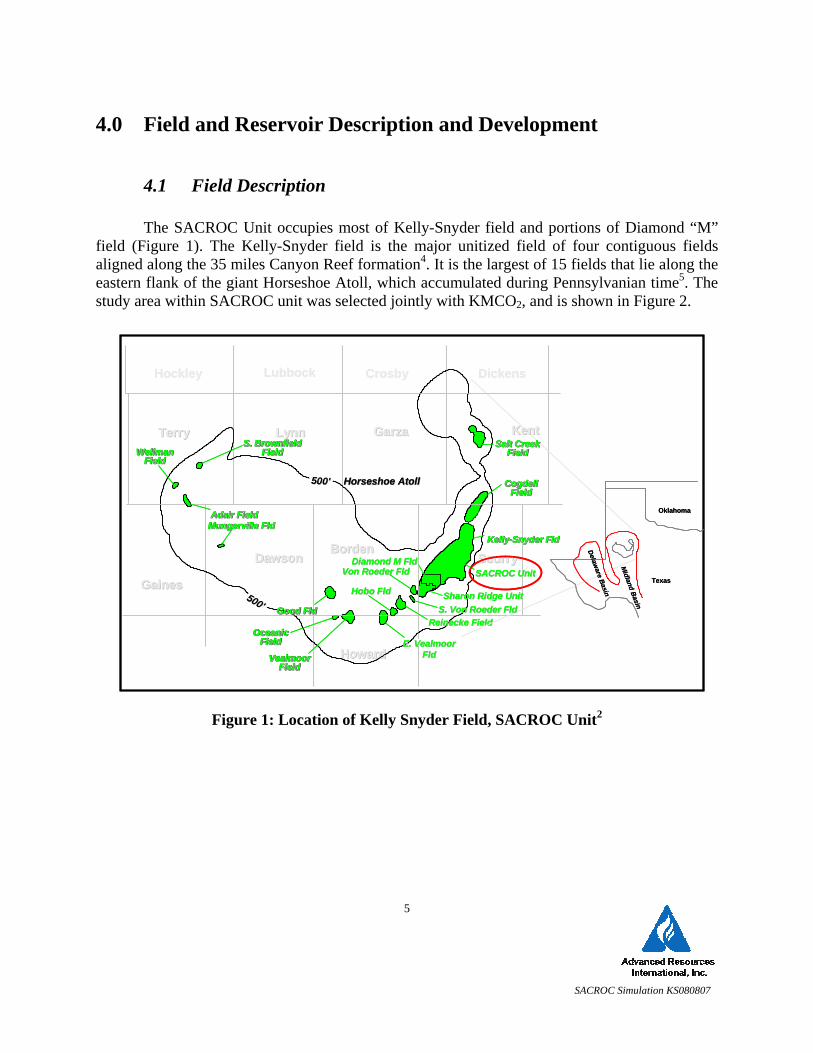
The SACROC Unit occupies most of Kelly-Snyder field and portions of Diamond “M” field (Figure 1). The Kelly-Snyder field is the major unitized field of four contiguous fields aligned along the 35 miles Canyon Reef formation4. It is the largest of 15 fields that lie along the eastern flank of the giant Horseshoe Atoll, which accumulated during Pennsylvanian time5. The study area within SACROC unit was selected jointly with KMCO2, and is shown in Figure 2.
Figure 1: Location of Kelly Snyder Field, SACROC Unit2
Hockley Lubbock Crosby Dickens
HowardHoward
TerryTerry LynnLynn GarzaGarza KentKent
GainesGaines
ScurryScurryDawsonDawsonBordenBorden
WellmanWellmanFieldField
WellmanWellmanFieldField
Adair FieldAdair FieldAdair FieldAdair Field
Hobo Hobo FldFld
OceanicOceanicFieldField
OceanicOceanicFieldField
VealmoorVealmoorFieldField
VealmoorVealmoorFieldField
CogdellCogdellFieldField
CogdellCogdellFieldField
S. BrownfieldS. BrownfieldFieldField
S. BrownfieldS. BrownfieldFieldField
MungervilleMungerville FldFldMungervilleMungerville FldFld
Von Roeder Von Roeder FldFld
Good Good FldFldGood Good FldFldReineckeReinecke FieldField
500'500'
500'500'
Sharon Ridge UnitSharon Ridge Unit
Diamond M Diamond M FldFld
KellyKelly--Snyder Snyder FldFldKellyKelly--Snyder Snyder FldFld
SACROC UnitSACROC Unit
Oklahoma
Texas
Midland Basin
S. Von Roeder S. Von Roeder FldFld
E. E. VealmoorVealmoorFldFld
Salt CreekSalt CreekFieldField
Salt CreekSalt CreekFieldField
Horseshoe AtollHorseshoe Atoll
Delaware Basin
Hockley Lubbock Crosby Dickens
HowardHoward
TerryTerry LynnLynn GarzaGarza KentKent
GainesGaines
ScurryScurryDawsonDawsonBordenBorden
WellmanWellmanFieldField
WellmanWellmanFieldField
Adair FieldAdair FieldAdair FieldAdair Field
Hobo Hobo FldFld
OceanicOceanicFieldField
OceanicOceanicFieldField
OceanicOceanicFieldField
OceanicOceanicFieldField
VealmoorVealmoorFieldField
VealmoorVealmoorFieldField
VealmoorVealmoorFieldField
VealmoorVealmoorFieldField
CogdellCogdellFieldField
CogdellCogdellFieldField
S. BrownfieldS. BrownfieldFieldField
S. BrownfieldS. BrownfieldFieldField
MungervilleMungerville FldFldMungervilleMungerville FldFld
Von Roeder Von Roeder FldFld
Good Good FldFldGood Good FldFldReineckeReinecke FieldField
500'500'
500'500'
Sharon Ridge UnitSharon Ridge Unit
Diamond M Diamond M FldFld
KellyKelly--Snyder Snyder FldFldKellyKelly--Snyder Snyder FldFld
SACROC UnitSACROC Unit
Oklahoma
Texas
Midland Basin
S. Von Roeder S. Von Roeder FldFld
E. E. VealmoorVealmoorFldFld
Salt CreekSalt CreekFieldField
Salt CreekSalt CreekFieldField
Horseshoe AtollHorseshoe Atoll
Delaware Basin
SACROC Simulation KS080807
6
Figure 2: Location of Study Area, Kelly Snyder Field2
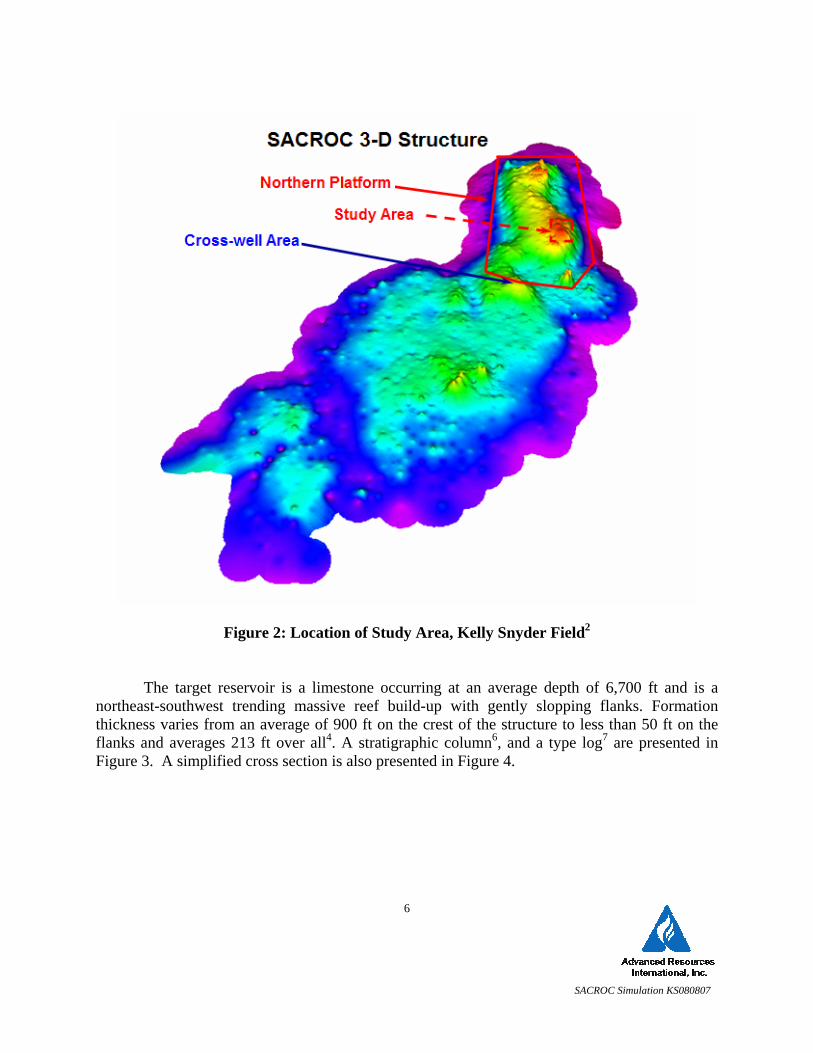
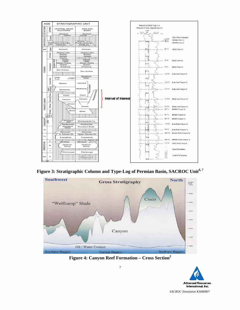
The target reservoir is a limestone occurring at an average depth of 6,700 ft and is a northeast-southwest trending massive reef build-up with gently slopping flanks. Formation thickness varies from an average of 900 ft on the crest of the structure to less than 50 ft on the flanks and averages 213 ft over all4. A stratigraphic column6, and a type log7 are presented in Figure 3. A simplified cross section is also presented in Figure 4.
SACROC Simulation KS080807
7
Figure 3: Stratigraphic Column and Type-Log of Permian Basin, SACROC Unit6, 7
Figure 4: Canyon Reef Formation – Cross Section2
Interval of InterestInterval of InterestInterval of InterestInterval of Interest
SACROC Simulation KS080807
8
The reservoir was discovered in November 1948 when Chevron Oil Co. completed the first well at a depth interval of 6,334 to 6,414 ft. This discovery was named the Kelly-Snyder field. Soon afterward, other operators discovered the Diamond “M” and Sharon Ridge Canyon fields to the south. Eventually, production revealed that the three fields merged to form one continuous reservoir. Subsequent development was rapid and essentially complete by November 1951 when 1617 producing wells had been drilled by 88 different operators5. By that time, reservoir pressure had declined by 50 percent after producing only 5% of the oil in place, and it was estimated that only 19% of the original oil in place would be recovered by primary depletion5. This indicated that solution gas drive was the primary producing mechanism and it was recognized that a pressure-maintenance program would be required to improve the recovery:.
In 1953, the Texas Railroad Commission approved formation of the SACROC (Scurry
Area Canyon Reef Operators Committee) Unit, which includes about 98 percent of Kelly-Snyder field, to facilitate coordinated water flooding operations. Water injection started in SACROC in September 1954 into 53 wells located along the longitudinal axis of the crest of the reef. This pattern is often referred as the “center-line” water flood in SACROC5.
The center-line water flood proved to be efficient because several independent reservoir
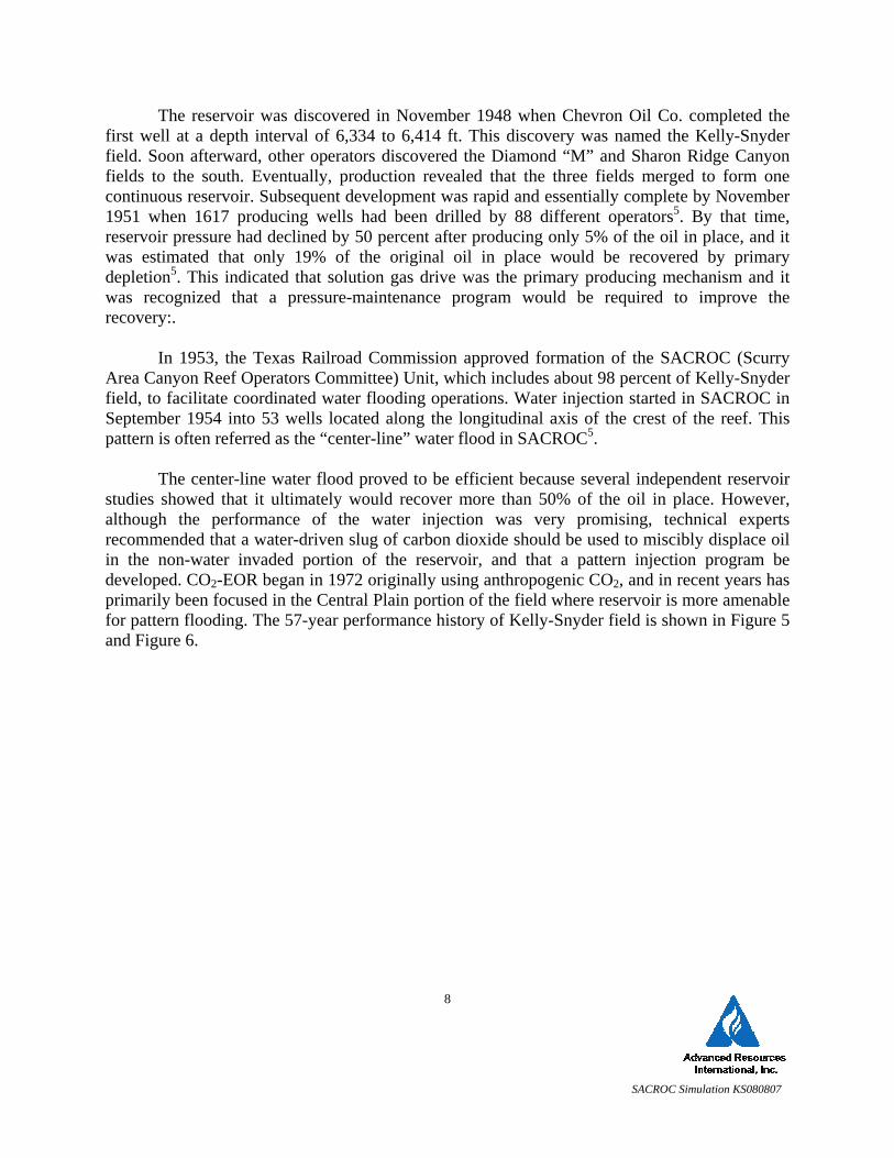
studies showed that it ultimately would recover more than 50% of the oil in place. However, although the performance of the water injection was very promising, technical experts recommended that a water-driven slug of carbon dioxide should be used to miscibly displace oil in the non-water invaded portion of the reservoir, and that a pattern injection program be developed. CO2-EOR began in 1972 originally using anthropogenic CO2, and in recent years has primarily been focused in the Central Plain portion of the field where reservoir is more amenable for pattern flooding. The 57-year performance history of Kelly-Snyder field is shown in Figure 5 and Figure 6.
SACROC Simulation KS080807
9
Figure 5: Kelly-Snyder Field Performance History6
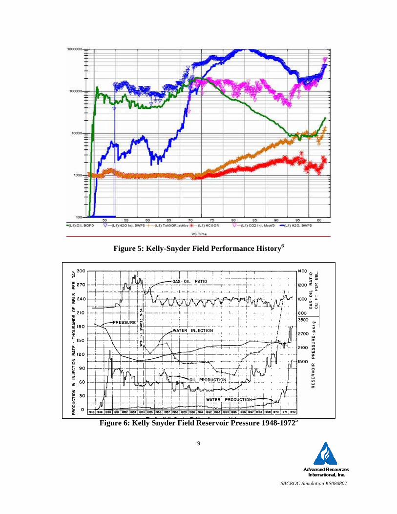
Figure 6: Kelly Snyder Field Reservoir Pressure 1948-19725
SACROC Simulation KS080807
10
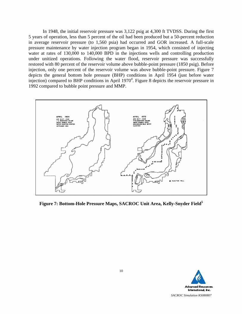
In 1948, the initial reservoir pressure was 3,122 psig at 4,300 ft TVDSS. During the first 5 years of operation, less than 5 percent of the oil had been produced but a 50-percent reduction in average reservoir pressure (to 1,560 psia) had occurred and GOR increased. A full-scale pressure maintenance by water injection program began in 1954, which consisted of injecting water at rates of 130,000 to 140,000 BPD in the injections wells and controlling production under unitized operations. Following the water flood, reservoir pressure was successfully restored with 80 percent of the reservoir volume above bubble-point pressure (1850 psig). Before injection, only one percent of the reservoir volume was above bubble-point pressure. Figure 7 depicts the general bottom hole pressure (BHP) conditions in April 1954 (just before water injection) compared to BHP conditions in April 19704. Figure 8 depicts the reservoir pressure in 1992 compared to bubble point pressure and MMP.
Figure 7: Bottom-Hole Pressure Maps, SACROC Unit Area, Kelly-Snyder Field5
SACROC Simulation KS080807
11
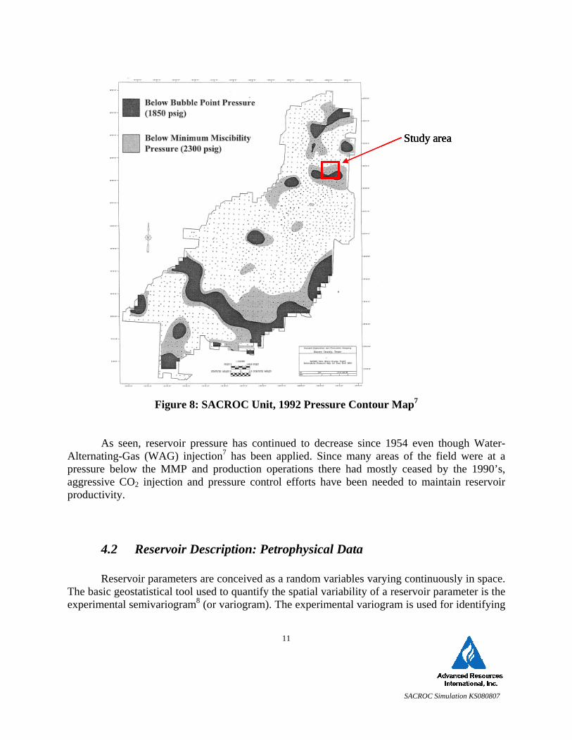
Figure 8: SACROC Unit, 1992 Pressure Contour Map7
As seen, reservoir pressure has continued to decrease since 1954 even though Water-Alternating-Gas (WAG) injection7 has been applied. Since many areas of the field were at a pressure below the MMP and production operations there had mostly ceased by the 1990’s, aggressive CO2 injection and pressure control efforts have been needed to maintain reservoir productivity.
4.2 Reservoir Description: Petrophysical Data
Reservoir parameters are conceived as a random variables varying continuously in space. The basic geostatistical tool used to quantify the spatial variability of a reservoir parameter is the experimental semivariogram8 (or variogram). The experimental variogram is used for identifying
Study areaStudy areaStudy area
SACROC Simulation KS080807
12
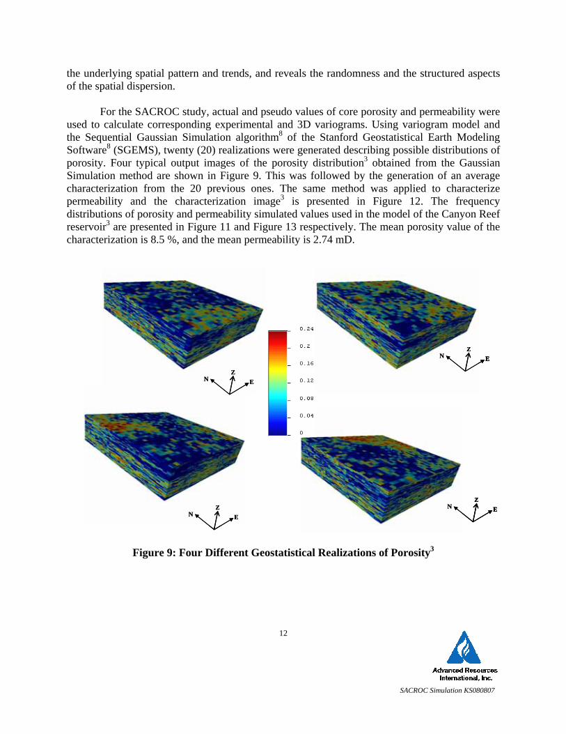
the underlying spatial pattern and trends, and reveals the randomness and the structured aspects of the spatial dispersion.
For the SACROC study, actual and pseudo values of core porosity and permeability were
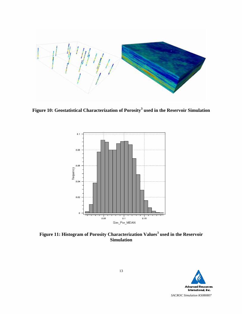
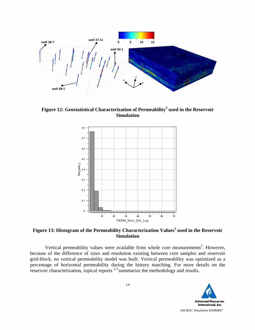
used to calculate corresponding experimental and 3D variograms. Using variogram model and the Sequential Gaussian Simulation algorithm8 of the Stanford Geostatistical Earth Modeling Software8 (SGEMS), twenty (20) realizations were generated describing possible distributions of porosity. Four typical output images of the porosity distribution3 obtained from the Gaussian Simulation method are shown in Figure 9. This was followed by the generation of an average characterization from the 20 previous ones. The same method was applied to characterize permeability and the characterization image3 is presented in Figure 12. The frequency distributions of porosity and permeability simulated values used in the model of the Canyon Reef reservoir3 are presented in Figure 11 and Figure 13 respectively. The mean porosity value of the characterization is 8.5 %, and the mean permeability is 2.74 mD.
Figure 9: Four Different Geostatistical Realizations of Porosity3
N EZ
N EZ N E
Z
N EZ
N EZ
N EZ
N EZ
N EZ N E
ZN E
Z
N EZ
N EZ
SACROC Simulation KS080807
13
Figure 10: Geostatistical Characterization of Porosity3 used in the Reservoir Simulation
Figure 11: Histogram of Porosity Characterization Values3 used in the Reservoir Simulation
SACROC Simulation KS080807
14
Figure 12: Geostatistical Characterization of Permeability3 used in the Reservoir
Simulation
Figure 13: Histogram of the Permeability Characterization Values3 used in the Reservoir Simulation
Vertical permeability values were available from whole core measurements2. However,
because of the difference of sizes and resolution existing between core samples and reservoir grid-block, no vertical permeability model was built. Vertical permeability was optimized as a percentage of horizontal permeability during the history matching. For more details on the reservoir characterization, topical reports 2,3 summarize the methodology and results.
Z
E N
well 37-11
well 62-1
well 36-7
well 58-1
0 5 10 15
SACROC Simulation KS080807
15
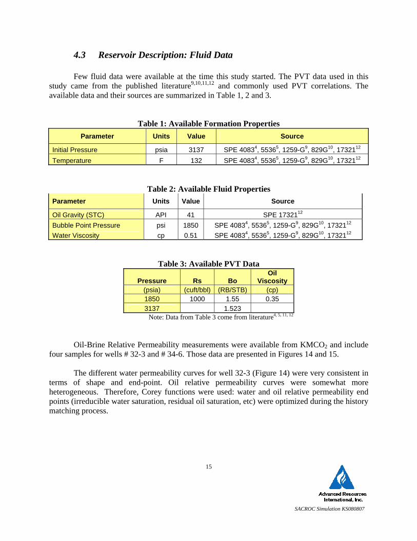
4.3 Reservoir Description: Fluid Data
Few fluid data were available at the time this study started. The PVT data used in this study came from the published literature9,10,11,12 and commonly used PVT correlations. The available data and their sources are summarized in Table 1, 2 and 3.
Table 1: Available Formation Properties Parameter Units Value Source
Initial Pressure psia 3137 SPE 40834, 55365, 1259-G9, 829G10, 1732112 Temperature F 132 SPE 40834, 55365, 1259-G9, 829G10, 1732112
Table 2: Available Fluid Properties Parameter Units Value Source
Oil Gravity (STC) API 41 SPE 1732112 Bubble Point Pressure psi 1850 SPE 40834, 55365, 1259-G9, 829G10, 1732112 Water Viscosity cp 0.51 SPE 40834, 55365, 1259-G9, 829G10, 1732112
Table 3: Available PVT Data
Pressure Rs Bo Oil
Viscosity (psia) (cuft/bbl) (RB/STB) (cp) 1850 1000 1.55 0.35 3137 1.523
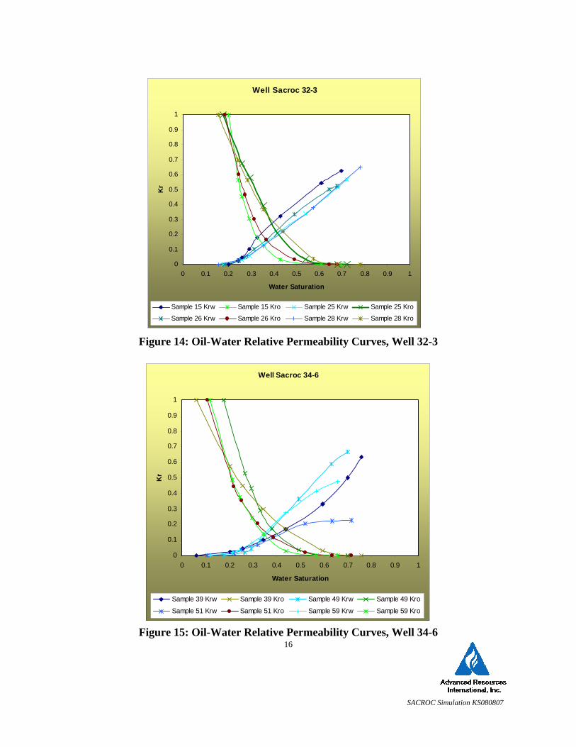
Note: Data from Table 3 come from literature4, 5, 11, 12 Oil-Brine Relative Permeability measurements were available from KMCO2 and include
four samples for wells # 32-3 and # 34-6. Those data are presented in Figures 14 and 15. The different water permeability curves for well 32-3 (Figure 14) were very consistent in
terms of shape and end-point. Oil relative permeability curves were somewhat more heterogeneous. Therefore, Corey functions were used: water and oil relative permeability end points (irreducible water saturation, residual oil saturation, etc) were optimized during the history matching process.
SACROC Simulation KS080807
16
Figure 14: Oil-Water Relative Permeability Curves, Well 32-3
Figure 15: Oil-Water Relative Permeability Curves, Well 34-6
Well Sacroc 32-3
0
0.1
0.2
0.3
0.4
0.5
0.6
0.7
0.8
0.9
1
0 0.1 0.2 0.3 0.4 0.5 0.6 0.7 0.8 0.9 1
Water Saturation
Kr
Sample 15 Krw Sample 15 Kro Sample 25 Krw Sample 25 Kro
Sample 26 Krw Sample 26 Kro Sample 28 Krw Sample 28 Kro
Well Sacroc 34-6
0
0.1
0.2
0.3
0.4
0.5
0.6
0.7
0.8
0.9
1
0 0.1 0.2 0.3 0.4 0.5 0.6 0.7 0.8 0.9 1
Water Saturation
Kr
Sample 39 Krw Sample 39 Kro Sample 49 Krw Sample 49 Kro
Sample 51 Krw Sample 51 Kro Sample 59 Krw Sample 59 Kro
SACROC Simulation KS080807
17
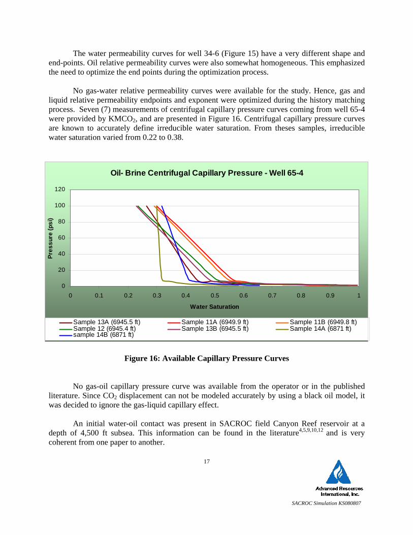
The water permeability curves for well 34-6 (Figure 15) have a very different shape and end-points. Oil relative permeability curves were also somewhat homogeneous. This emphasized the need to optimize the end points during the optimization process.
No gas-water relative permeability curves were available for the study. Hence, gas and
liquid relative permeability endpoints and exponent were optimized during the history matching process. Seven (7) measurements of centrifugal capillary pressure curves coming from well 65-4 were provided by KMCO2, and are presented in Figure 16. Centrifugal capillary pressure curves are known to accurately define irreducible water saturation. From theses samples, irreducible water saturation varied from 0.22 to 0.38.
Figure 16: Available Capillary Pressure Curves
No gas-oil capillary pressure curve was available from the operator or in the published literature. Since CO2 displacement can not be modeled accurately by using a black oil model, it was decided to ignore the gas-liquid capillary effect.
An initial water-oil contact was present in SACROC field Canyon Reef reservoir at a
depth of 4,500 ft subsea. This information can be found in the literature4,5,9,10,12 and is very coherent from one paper to another.
Oil- Brine Centrifugal Capillary Pressure - Well 65-4
0
20
40
60
80
100
120
0 0.1 0.2 0.3 0.4 0.5 0.6 0.7 0.8 0.9 1
Water Saturation
Pres
sure
(psi
)
Sample 13A (6945.5 ft) Sample 11A (6949.9 ft) Sample 11B (6949.8 ft)Sample 12 (6945.4 ft) Sample 13B (6945.5 ft) Sample 14A (6871 ft)sample 14B (6871 ft)
SACROC Simulation KS080807
18
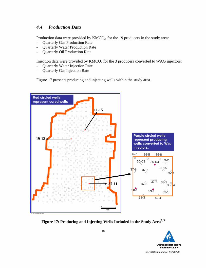
4.4 Production Data
Production data were provided by KMCO2 for the 19 producers in the study area: - Quarterly Gas Production Rate - Quarterly Water Production Rate - Quarterly Oil Production Rate
Injection data were provided by KMCO2 for the 3 producers converted to WAG injectors: - Quarterly Water Injection Rate - Quarterly Gas Injection Rate
Figure 17 presents producing and injecting wells within the study area.
Figure 17: Producing and Injecting Wells Included in the Study Area2, 3
4,249
33-11
33-1433-1
33-15
33-2
36-5 36-7 36-8
36-C3 36-D4
37-4
37-5
37-6
37-8
58-1
58-3
59-1
59-4
62-1
Red circled wells represent cored wells
37-11
11-15
FEE
0
PETRA 2/28/2006 11:08:44 AM
19-12 Purple circled wells represent producing wells converted to Wag injectors.
SACROC Simulation KS080807
19
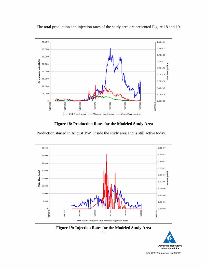
The total production and injection rates of the study area are presented Figure 18 and 19.
Figure 18: Production Rates for the Modeled Study Area
Production started in August 1949 inside the study area and is still active today.
Figure 19: Injection Rates for the Modeled Study Area
0
5,000
10,000
15,000
20,000
25,000
30,000
35,000
40,000
7/17
/194
6
7/14
/195
6
7/12
/196
6
7/9/
1976
7/7/
1986
7/4/
1996
7/2/
2006
6/29
/201
6
Oil
and
Wat
er ra
te (b
bl/d
)
0.0E+00
2.0E+06
4.0E+06
6.0E+06
8.0E+06
1.0E+07
1.2E+07
1.4E+07
1.6E+07
1.8E+07
Gas
Rat
e (c
uft/d
)
Oil Production Water production Gas Production
0
5,000
10,000
15,000
20,000
25,000
30,000
35,000
40,000
7/17
/194
6
7/14
/195
6
7/12
/196
6
7/9/
1976
7/7/
1986
7/4/
1996
7/2/
2006
6/29
/201
6
Wat
er R
ate
(bbl
/d)
0.0E+00
2.0E+06
4.0E+06
6.0E+06
8.0E+06
1.0E+07
1.2E+07
1.4E+07
1.6E+07
1.8E+07
Gas
Rat
e (c
uft/d
)
Water injection rate Gas Injection Rate

SACROC Simulation KS080807
20
Water injection started in April 1961 and was then converted to WAG13 in July 1973 inside the study area. WAG injection is still active today on the Northern Platform. Gas injection stopped in August 1996 inside the study area.
SACROC Simulation KS080807
21
5.0 Reservoir Simulation
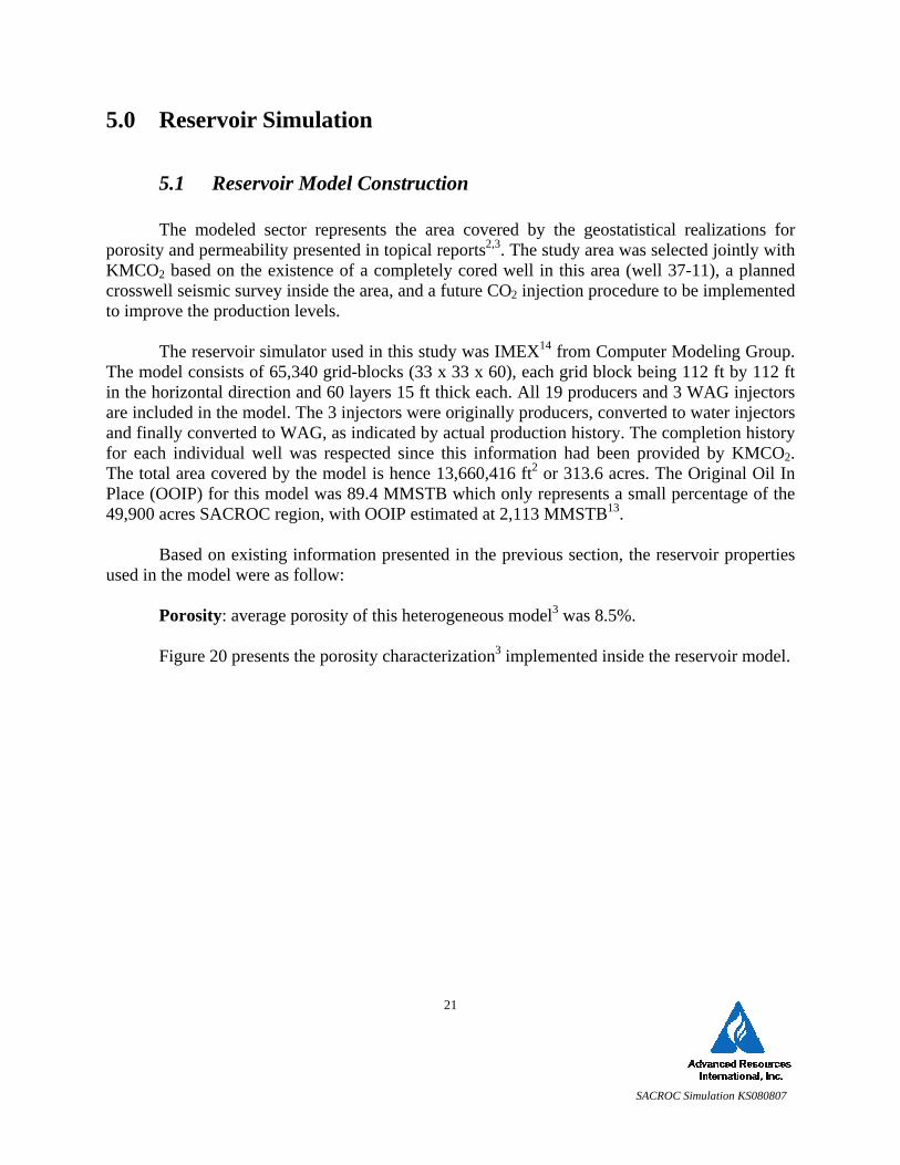
5.1 Reservoir Model Construction
The modeled sector represents the area covered by the geostatistical realizations for porosity and permeability presented in topical reports2,3. The study area was selected jointly with KMCO2 based on the existence of a completely cored well in this area (well 37-11), a planned crosswell seismic survey inside the area, and a future CO2 injection procedure to be implemented to improve the production levels.
The reservoir simulator used in this study was IMEX14 from Computer Modeling Group.
The model consists of 65,340 grid-blocks (33 x 33 x 60), each grid block being 112 ft by 112 ft in the horizontal direction and 60 layers 15 ft thick each. All 19 producers and 3 WAG injectors are included in the model. The 3 injectors were originally producers, converted to water injectors and finally converted to WAG, as indicated by actual production history. The completion history for each individual well was respected since this information had been provided by KMCO2. The total area covered by the model is hence 13,660,416 ft2 or 313.6 acres. The Original Oil In Place (OOIP) for this model was 89.4 MMSTB which only represents a small percentage of the 49,900 acres SACROC region, with OOIP estimated at 2,113 MMSTB13.
Based on existing information presented in the previous section, the reservoir properties used in the model were as follow:
Porosity: average porosity of this heterogeneous model3 was 8.5%. Figure 20 presents the porosity characterization3 implemented inside the reservoir model.
SACROC Simulation KS080807
22
Figure 20: Porosity Model of the Study Area
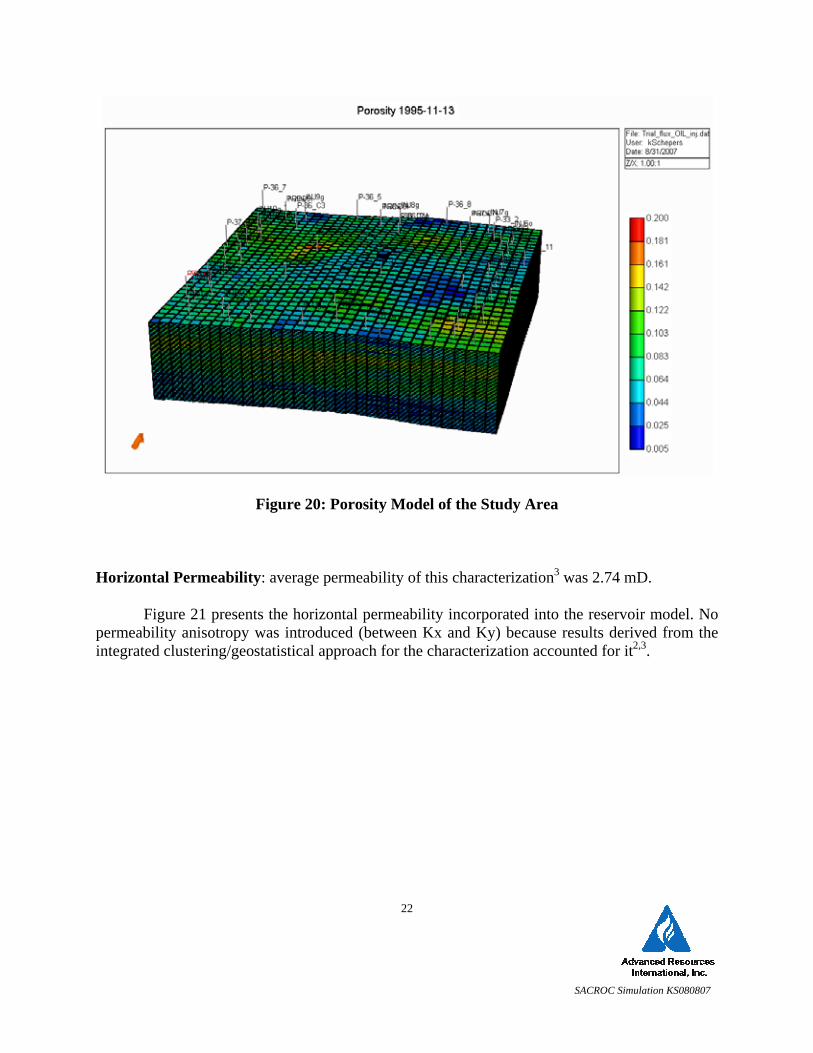
Horizontal Permeability: average permeability of this characterization3 was 2.74 mD.
Figure 21 presents the horizontal permeability incorporated into the reservoir model. No permeability anisotropy was introduced (between Kx and Ky) because results derived from the integrated clustering/geostatistical approach for the characterization accounted for it2,3.
SACROC Simulation KS080807
23
Figure 21: Horizontal Permeability Model of the Study Area
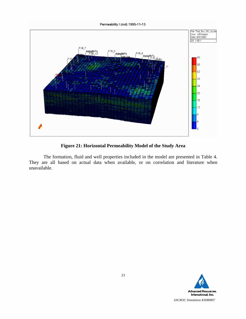
The formation, fluid and well properties included in the model are presented in Table 4.
They are all based on actual data when available, or on correlation and literature when unavailable.
SACROC Simulation KS080807
24
Table 4: Formation, Fluid and Well Properties of the Reservoir Model Parameter Units Value Reference Depth/Pressure
Formation Properties Initial Pressure psia 3137 at 4300ft TVDSS (actual data) Initial Temperature F 132 at 4300ft TVDSS (actual data) Initial Water Oil Contact FT 4500 TVDSS (actual data) Rock Compressibility 1/psi 5.60E-06 at 3137 psia (actual data)
Fluid Properties Bubble Point Pressure psi 1850 at 4300ft TVDSS (actual data) Oil Compressibility 1/psi 7.00E-05 at 1850 psia (Ramey's correlation15)
Oil Density API 37.2 at STC (actual data and Mc Cain's
correlation16) Gas Gravity - 0.67 at STC (Standing and Katz's correlation17)
Water Compressibility 1/psi 2.90E-06 at 1850 psia ( Dodson and Standing's
correlation18) Water Density - 62.3 (Earlougher, R.C.19) Water FVF RB/STB 1.013 (Rowe and Chou's correlation20)
Water Viscosity cp 0.51 (actual data and Matthews and Russell's
correlation21) Relative Permeability Relationships Krliq - 1 assumed Well Parameters Skin Producers - -1 assumed Skin injectors - -1 assumed
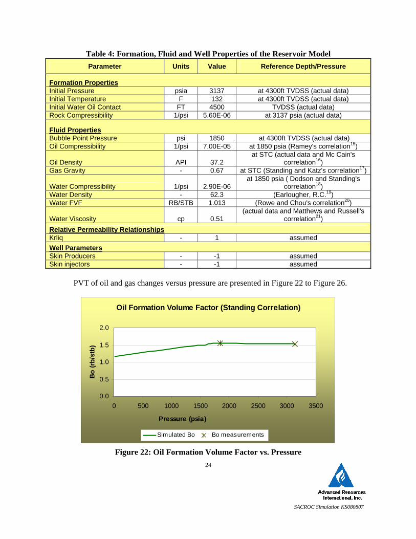
PVT of oil and gas changes versus pressure are presented in Figure 22 to Figure 26.
Figure 22: Oil Formation Volume Factor vs. Pressure
Oil Formation Volume Factor (Standing Correlation)
0.0
0.5
1.0
1.5
2.0
0 500 1000 1500 2000 2500 3000 3500
Pressure (psia)
Bo
(rb/s
tb)
Simulated Bo Bo measurements
SACROC Simulation KS080807
25
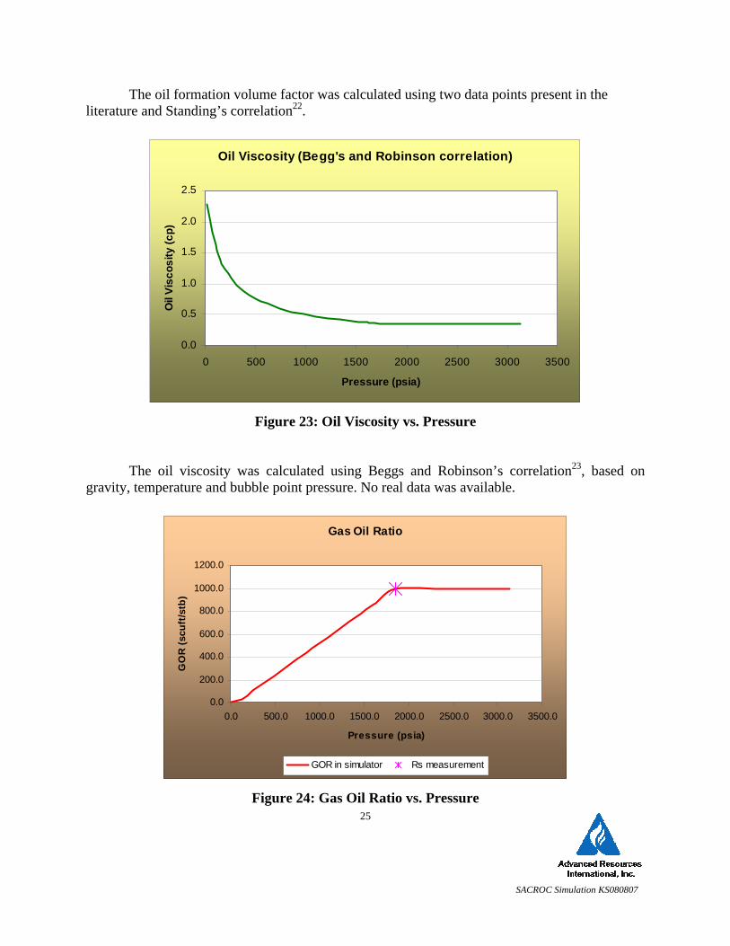
The oil formation volume factor was calculated using two data points present in the literature and Standing’s correlation22.
Figure 23: Oil Viscosity vs. Pressure
The oil viscosity was calculated using Beggs and Robinson’s correlation23, based on gravity, temperature and bubble point pressure. No real data was available.
Figure 24: Gas Oil Ratio vs. Pressure
Oil Viscosity (Begg's and Robinson correlation)
0.0
0.5
1.0
1.5
2.0
2.5
0 500 1000 1500 2000 2500 3000 3500
Pressure (psia)
Oil
Visc
osity
(cp)
Gas Oil Ratio
0.0
200.0
400.0
600.0
800.0
1000.0
1200.0
0.0 500.0 1000.0 1500.0 2000.0 2500.0 3000.0 3500.0
Pressure (psia)
GO
R (s
cuft
/stb
)
GOR in simulator Rs measurement
SACROC Simulation KS080807
26
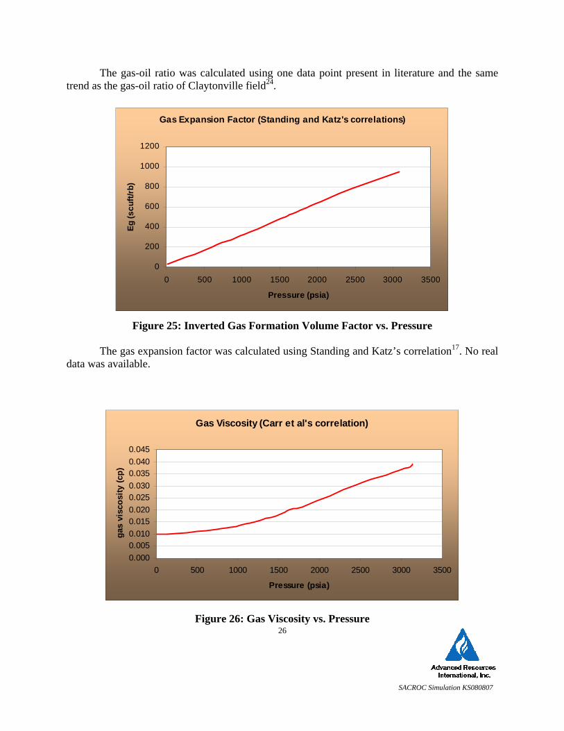
The gas-oil ratio was calculated using one data point present in literature and the same trend as the gas-oil ratio of Claytonville field24.
Figure 25: Inverted Gas Formation Volume Factor vs. Pressure
The gas expansion factor was calculated using Standing and Katz’s correlation17. No real data was available.
Figure 26: Gas Viscosity vs. Pressure
Gas Expansion Factor (Standing and Katz's correlations)
0
200
400
600
800
1000
1200
0 500 1000 1500 2000 2500 3000 3500
Pressure (psia)
Eg (s
cuft/
rb)
Gas Viscosity (Carr et al's correlation)
0.0000.0050.0100.0150.0200.0250.0300.0350.0400.045
0 500 1000 1500 2000 2500 3000 3500
Pressure (psia)
gas
visc
osity
(cp)
SACROC Simulation KS080807
27
No gas viscosity data was available; therefore, it was calculated using Carr et al’s correlation25. Only one rock type was defined in this model. From the relative permeability samples of wells 32-3 and 34-3, relative permeability (Kr) curves endpoints vary significantly, so it was decided to vary oil-water and gas-liquid relative permeability endpoints and shape using Corey’s functions during the optimization process.
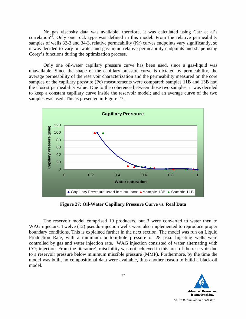
Only one oil-water capillary pressure curve has been used, since a gas-liquid was
unavailable. Since the shape of the capillary pressure curve is dictated by permeability, the average permeability of the reservoir characterization and the permeability measured on the core samples of the capillary pressure (Pc) measurements were compared: samples 11B and 13B had the closest permeability value. Due to the coherence between those two samples, it was decided to keep a constant capillary curve inside the reservoir model; and an average curve of the two samples was used. This is presented in Figure 27.
Figure 27: Oil-Water Capillary Pressure Curve vs. Real Data
The reservoir model comprised 19 producers, but 3 were converted to water then to WAG injectors. Twelve (12) pseudo-injection wells were also implemented to reproduce proper boundary conditions. This is explained further in the next section. The model was run on Liquid Production Rate, with a minimum bottom-hole pressure of 28 psia. Injecting wells were controlled by gas and water injection rate. WAG injection consisted of water alternating with CO2 injection. From the literature7, miscibility was not achieved in this area of the reservoir due to a reservoir pressure below minimum miscible pressure (MMP). Furthermore, by the time the model was built, no compositional data were available, thus another reason to build a black-oil model.
Capillary Pressure
0
20
40
60
80
100
120
0 0.2 0.4 0.6 0.8 1
Water saturation
Cap
illar
y Pr
essu
re (p
sia)
Capillary Pressure used in simulator sample 13B Sample 11B

SACROC Simulation KS080807
28
Because a black-oil model was used, proper CO2 behavior could not be accurately reproduced. To address this issue:
- Injected gas composition was specified as CO2: this allowed modeling accurate CO2 flows inside the wellbore.
- Inside the reservoir, properties of a lean miscible gas were used for injected gas phase (only option available in black oil model).
This definitely had an impact on the recovery factor, but it ended up not being as critical
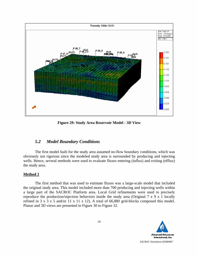
as it will be presented in the Section 6.3 (Results) of this report. Figure 28 and Figure 29 present respectively a planar section (layer 17) and a 3D view of the current reservoir porosity model.
Figure 28: Study Area Reservoir Model - Top View
SACROC Simulation KS080807
29
Figure 29: Study Area Reservoir Model - 3D View
5.2 Model Boundary Conditions
The first model built for the study area assumed no-flow boundary conditions, which was obviously not rigorous since the modeled study area is surrounded by producing and injecting wells. Hence, several methods were used to evaluate fluxes entering (influx) and exiting (efflux) the study area. Method 1
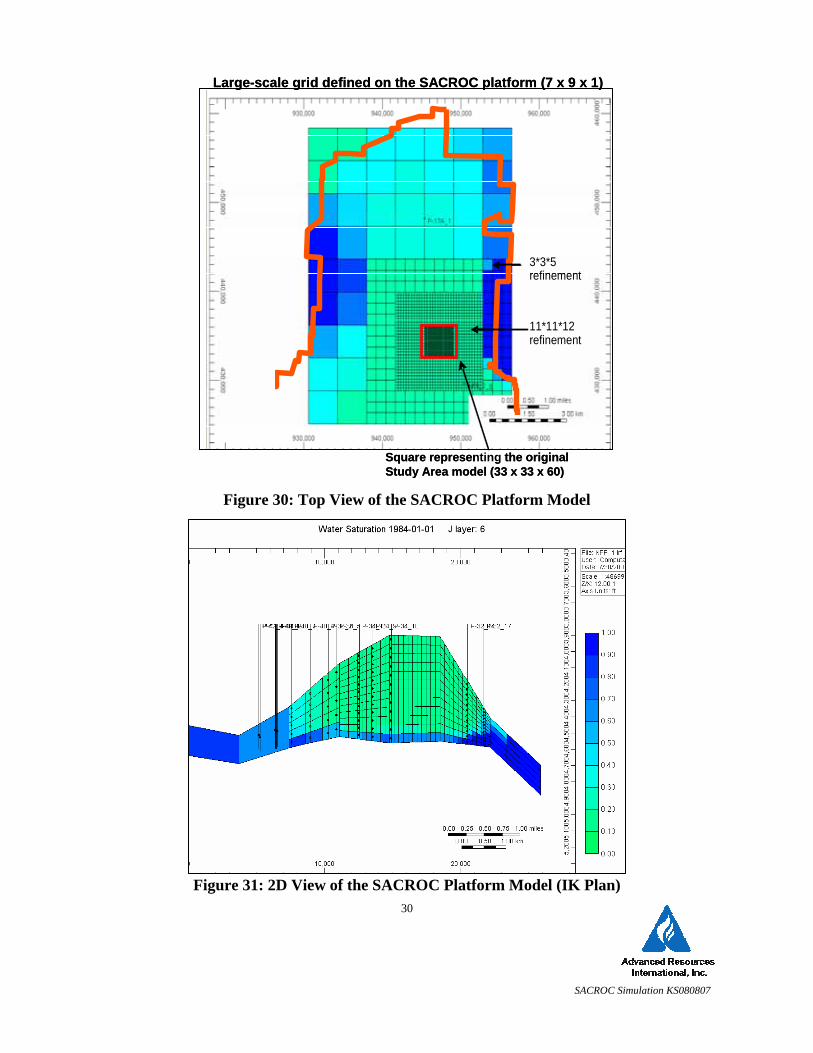
The first method that was used to estimate fluxes was a large-scale model that included the original study area. This model included more than 700 producing and injecting wells within a large part of the SACROC Platform area. Local Grid refinements were used to precisely reproduce the production/injection behaviors inside the study area (Original 7 x 9 x 1 locally refined in 3 x 3 x 5 and/or 11 x 11 x 12). A total of 66,880 grid-blocks composed this model. Planar and 3D views are presented in Figure 30 to Figure 32.
SACROC Simulation KS080807
30
Figure 30: Top View of the SACROC Platform Model
Figure 31: 2D View of the SACROC Platform Model (IK Plan)
11*11*12 refinement
3*3*5 refinement
Large-scale grid defined on the SACROC platform (7 x 9 x 1)
Square representing the original Study Area model (33 x 33 x 60)
11*11*12 refinement
3*3*5 refinement
Large-scale grid defined on the SACROC platform (7 x 9 x 1)
Square representing the original Study Area model (33 x 33 x 60)
SACROC Simulation KS080807
31
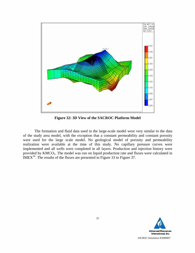
Figure 32: 3D View of the SACROC Platform Model
The formation and fluid data used in the large-scale model were very similar to the data of the study area model, with the exception that a constant permeability and constant porosity were used for the large scale model. No geological model of porosity and permeability realization were available at the time of this study. No capillary pressure curves were implemented and all wells were completed in all layers. Production and injection history were provided by KMCO2. The model was run on liquid production rate and fluxes were calculated in IMEX14. The results of the fluxes are presented in Figure 33 to Figure 37.
SACROC Simulation KS080807
32
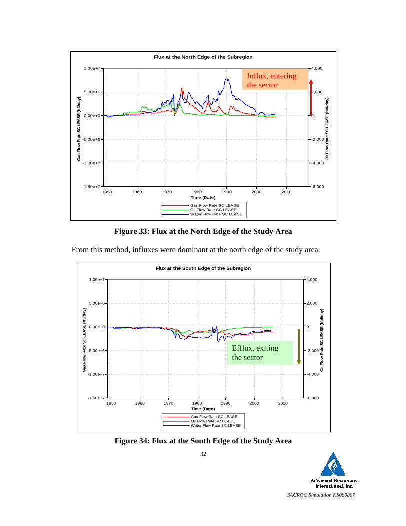
Figure 33: Flux at the North Edge of the Study Area
From this method, influxes were dominant at the north edge of the study area.
Figure 34: Flux at the South Edge of the Study Area
Flux at the North Edge of the Subregion
Gas Flow Rate SC LEASE Oil Flow Rate SC LEASE Water Flow Rate SC LEASE
Time (Date)
Gas
Flo
w R
ate
SC L
EASE
(ft3
/day
)
Oil
Flow
Rat
e SC
LEA
SE (b
bl/d
ay)
1950 1960 1970 1980 1990 2000 2010-1.50e+7
-1.00e+7
-5.00e+6
0.00e+0
5.00e+6
1.00e+7
-6,000
-4,000
-2,000
0
2,000
4,000
Influx, entering the sector
Flux at the South Edge of the Subregion
Gas Flow Rate SC LEASE Oil Flow Rate SC LEASE Water Flow Rate SC LEASE
Time (Date)
Gas
Flo
w R
ate
SC L
EASE
(ft3
/day
)
Oil
Flow
Rat
e SC
LEA
SE (b
bl/d
ay)
1950 1960 1970 1980 1990 2000 2010-1.50e+7
-1.00e+7
-5.00e+6
0.00e+0
5.00e+6
1.00e+7
-6,000
-4,000
-2,000
0
2,000
4,000
Efflux, exiting the sector
SACROC Simulation KS080807
33
At the south edge of the study area, effluxes were dominant but not as large as at the north edge.
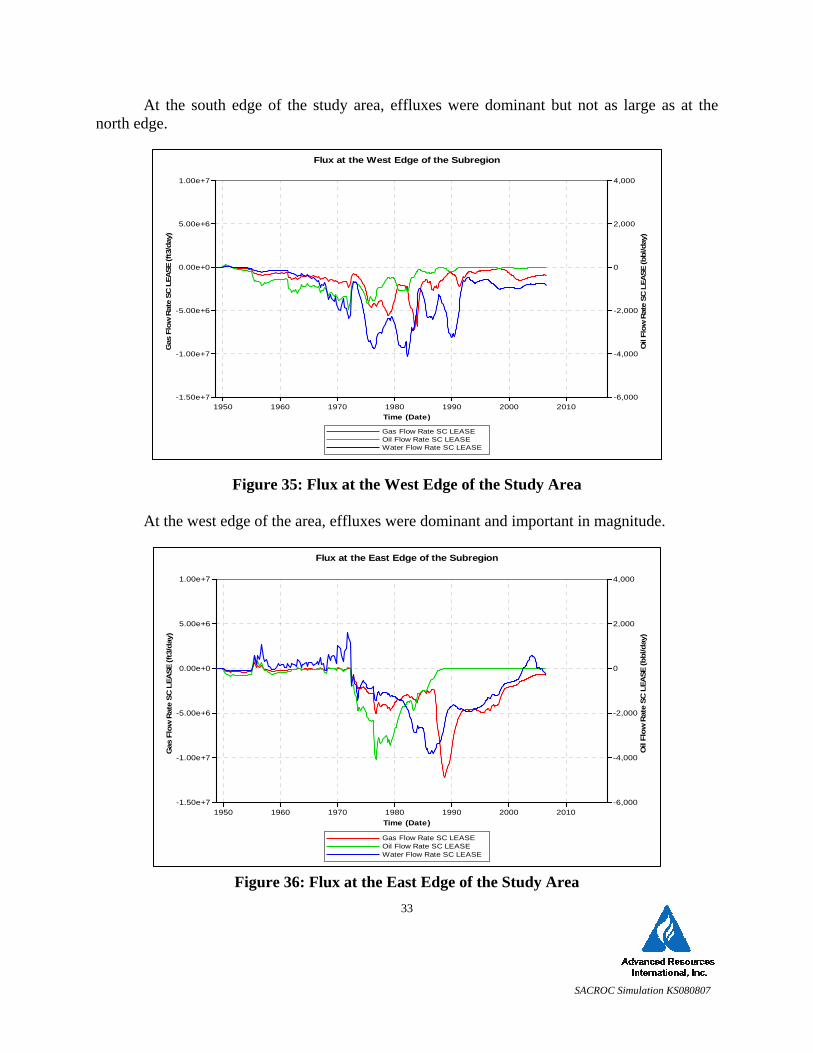
Figure 35: Flux at the West Edge of the Study Area
At the west edge of the area, effluxes were dominant and important in magnitude.
Figure 36: Flux at the East Edge of the Study Area
Flux at the East Edge of the Subregion
Gas Flow Rate SC LEASE Oil Flow Rate SC LEASE Water Flow Rate SC LEASE
Time (Date)
Gas
Flo
w R
ate
SC L
EASE
(ft3
/day
)
Oil
Flow
Rat
e SC
LEA
SE (b
bl/d
ay)
1950 1960 1970 1980 1990 2000 2010-1.50e+7
-1.00e+7
-5.00e+6
0.00e+0
5.00e+6
1.00e+7
-6,000
-4,000
-2,000
0
2,000
4,000
Flux at the West Edge of the Subregion
Gas Flow Rate SC LEASE Oil Flow Rate SC LEASE Water Flow Rate SC LEASE
Time (Date)
Gas
Flo
w R
ate
SC L
EASE
(ft3
/day
)
Oil
Flow
Rat
e SC
LEA
SE (b
bl/d
ay)
1950 1960 1970 1980 1990 2000 2010-1.50e+7
-1.00e+7
-5.00e+6
0.00e+0
5.00e+6
1.00e+7
-6,000
-4,000
-2,000
0
2,000
4,000
SACROC Simulation KS080807
34
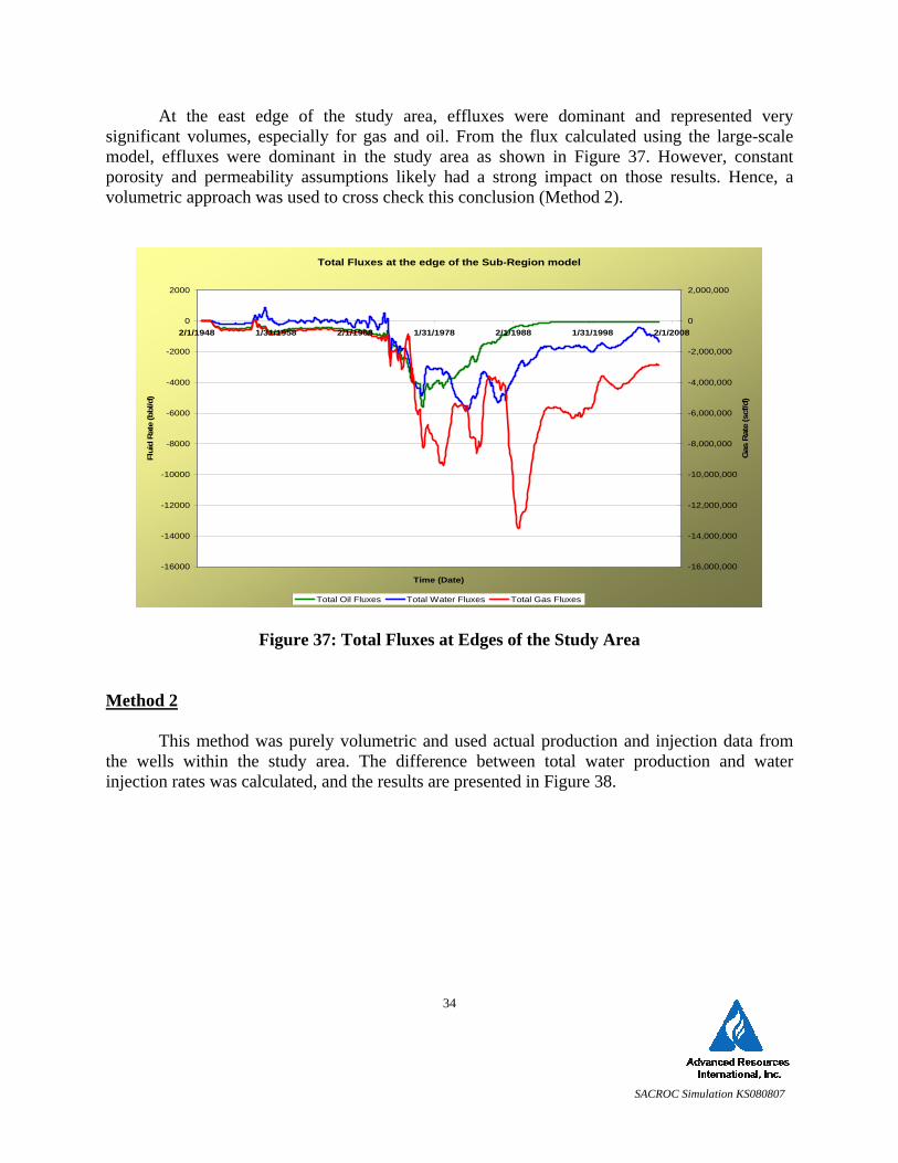
At the east edge of the study area, effluxes were dominant and represented very significant volumes, especially for gas and oil. From the flux calculated using the large-scale model, effluxes were dominant in the study area as shown in Figure 37. However, constant porosity and permeability assumptions likely had a strong impact on those results. Hence, a volumetric approach was used to cross check this conclusion (Method 2).
Figure 37: Total Fluxes at Edges of the Study Area
Method 2
This method was purely volumetric and used actual production and injection data from the wells within the study area. The difference between total water production and water injection rates was calculated, and the results are presented in Figure 38.
Total Fluxes at the edge of the Sub-Region model
-16000
-14000
-12000
-10000
-8000
-6000
-4000
-2000
0
2000
2/1/1948 1/31/1958 2/1/1968 1/31/1978 2/1/1988 1/31/1998 2/1/2008
Time (Date)
Flui
d R
ate
(bbl
/d)
-16,000,000
-14,000,000
-12,000,000
-10,000,000
-8,000,000
-6,000,000
-4,000,000
-2,000,000
0
2,000,000
Gas
Rat
e (s
cf/d
)
Total Oil Fluxes Total Water Fluxes Total Gas Fluxes
SACROC Simulation KS080807
35
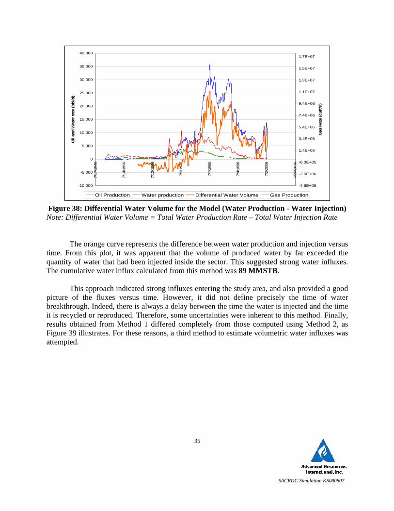
Figure 38: Differential Water Volume for the Model (Water Production - Water Injection) Note: Differential Water Volume = Total Water Production Rate – Total Water Injection Rate
The orange curve represents the difference between water production and injection versus time. From this plot, it was apparent that the volume of produced water by far exceeded the quantity of water that had been injected inside the sector. This suggested strong water influxes. The cumulative water influx calculated from this method was 89 MMSTB.
This approach indicated strong influxes entering the study area, and also provided a good
picture of the fluxes versus time. However, it did not define precisely the time of water breakthrough. Indeed, there is always a delay between the time the water is injected and the time it is recycled or reproduced. Therefore, some uncertainties were inherent to this method. Finally, results obtained from Method 1 differed completely from those computed using Method 2, as Figure 39 illustrates. For these reasons, a third method to estimate volumetric water influxes was attempted.
-10,000
-5,000
0
5,000
10,000
15,000
20,000
25,000
30,000
35,000
40,000
7/17
/194
6
7/14
/195
6
7/12
/196
6
7/9/
1976
7/7/
1986
7/4/
1996
7/2/
2006
6/29
/201
6
Oil
and
Wat
er ra
te (b
bl/d
)
-4.6E+06
-2.6E+06
-6.0E+05
1.4E+06
3.4E+06
5.4E+06
7.4E+06
9.4E+06
1.1E+07
1.3E+07
1.5E+07
1.7E+07
Gas
Rat
e (c
uft/d
)
Oil Production Water production Differential Water Volume Gas Production
SACROC Simulation KS080807
36
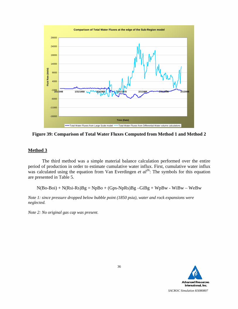
Figure 39: Comparison of Total Water Fluxes Computed from Method 1 and Method 2 Method 3
The third method was a simple material balance calculation performed over the entire period of production in order to estimate cumulative water influx. First, cumulative water influx was calculated using the equation from Van Everdingen et al26: The symbols for this equation are presented in Table 5.
N(Bo-Boi) + N(Rsi-Rs)Bg = NpBo + (Gps-NpRs)Bg –GiBg + WpBw - WiBw – WeBw Note 1: since pressure dropped below bubble point (1850 psia), water and rock expansions were neglected. Note 2: No original gas cap was present.
Comparison of Total Water Fluxes at the edge of the Sub-Region model
-16000
-11000
-6000
-1000
4000
9000
14000
19000
24000
29000
2/1/1948 1/31/1958 2/1/1968 1/31/1978 2/1/1988 1/31/1998 2/1/2008
Time (Date)
Flui
d R
ate
(bbl
/d)
Total Water Fluxes from Large Scale model Total Water Fluxes from Differential Water volume calculations
SACROC Simulation KS080807
37
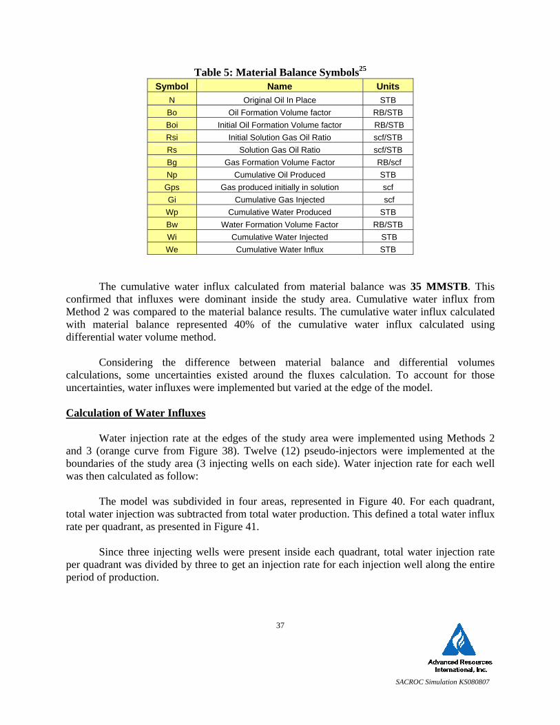
Table 5: Material Balance Symbols25 Symbol Name Units
N Original Oil In Place STB Bo Oil Formation Volume factor RB/STB Boi Initial Oil Formation Volume factor RB/STB Rsi Initial Solution Gas Oil Ratio scf/STB Rs Solution Gas Oil Ratio scf/STB Bg Gas Formation Volume Factor RB/scf Np Cumulative Oil Produced STB
Gps Gas produced initially in solution scf Gi Cumulative Gas Injected scf Wp Cumulative Water Produced STB Bw Water Formation Volume Factor RB/STB Wi Cumulative Water Injected STB We Cumulative Water Influx STB
The cumulative water influx calculated from material balance was 35 MMSTB. This confirmed that influxes were dominant inside the study area. Cumulative water influx from Method 2 was compared to the material balance results. The cumulative water influx calculated with material balance represented 40% of the cumulative water influx calculated using differential water volume method.
Considering the difference between material balance and differential volumes
calculations, some uncertainties existed around the fluxes calculation. To account for those uncertainties, water influxes were implemented but varied at the edge of the model. Calculation of Water Influxes
Water injection rate at the edges of the study area were implemented using Methods 2 and 3 (orange curve from Figure 38). Twelve (12) pseudo-injectors were implemented at the boundaries of the study area (3 injecting wells on each side). Water injection rate for each well was then calculated as follow:
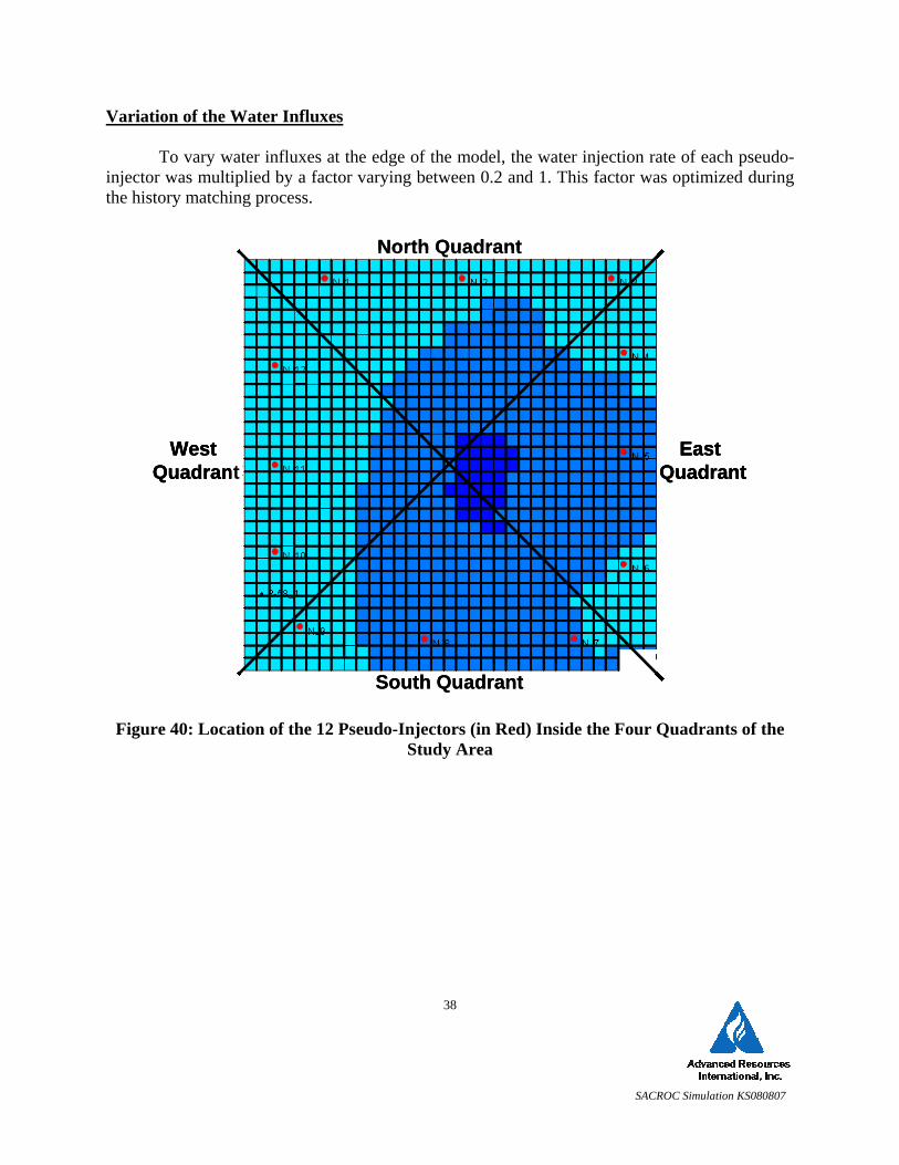
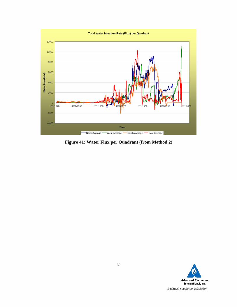
The model was subdivided in four areas, represented in Figure 40. For each quadrant,
total water injection was subtracted from total water production. This defined a total water influx rate per quadrant, as presented in Figure 41.
Since three injecting wells were present inside each quadrant, total water injection rate
per quadrant was divided by three to get an injection rate for each injection well along the entire period of production.
SACROC Simulation KS080807
38
Variation of the Water Influxes To vary water influxes at the edge of the model, the water injection rate of each pseudo-
injector was multiplied by a factor varying between 0.2 and 1. This factor was optimized during the history matching process.
Figure 40: Location of the 12 Pseudo-Injectors (in Red) Inside the Four Quadrants of the
Study Area
t t t t East
QuadrantWest
Quadrant
North Quadrant
South Quadrant
t t t t East
QuadrantWest
Quadrantt t t t East
QuadrantWest
Quadrant
North Quadrant
South Quadrant
SACROC Simulation KS080807
39
Figure 41: Water Flux per Quadrant (from Method 2)
Total Water Injection Rate (Flux) per Quadrant
-4000
-2000
0
2000
4000
6000
8000
10000
12000
2/1/1948 1/31/1958 2/1/1968 1/31/1978 2/1/1988 1/31/1998 2/1/2008
Time
Wat
er R
ate
(bbl
/d)
North Average West Average South Average East Average
SACROC Simulation KS080807
40
6.0 History Matching
6.1 Procedure
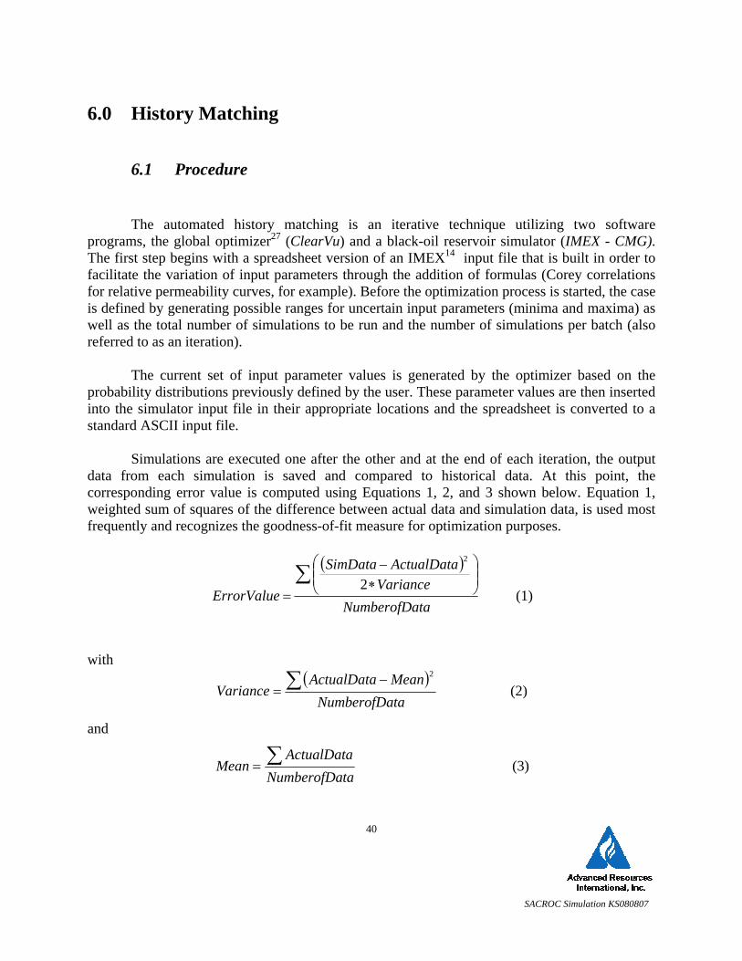
The automated history matching is an iterative technique utilizing two software programs, the global optimizer27 (ClearVu) and a black-oil reservoir simulator (IMEX - CMG). The first step begins with a spreadsheet version of an IMEX14 input file that is built in order to facilitate the variation of input parameters through the addition of formulas (Corey correlations for relative permeability curves, for example). Before the optimization process is started, the case is defined by generating possible ranges for uncertain input parameters (minima and maxima) as well as the total number of simulations to be run and the number of simulations per batch (also referred to as an iteration).
The current set of input parameter values is generated by the optimizer based on the
probability distributions previously defined by the user. These parameter values are then inserted into the simulator input file in their appropriate locations and the spreadsheet is converted to a standard ASCII input file.
Simulations are executed one after the other and at the end of each iteration, the output
data from each simulation is saved and compared to historical data. At this point, the corresponding error value is computed using Equations 1, 2, and 3 shown below. Equation 1, weighted sum of squares of the difference between actual data and simulation data, is used most frequently and recognizes the goodness-of-fit measure for optimization purposes.
( )
taNumberofDaVariance
ActualDataSimData
ErrorValue∑ ⎟⎟
⎠
⎞⎜⎜⎝
⎛∗−
=2
2
(1)
with
( )taNumberofDaMeanActualData
Variance ∑ −=
2
(2)
and
taNumberofDaActualData
Mean ∑= (3)
SACROC Simulation KS080807
41
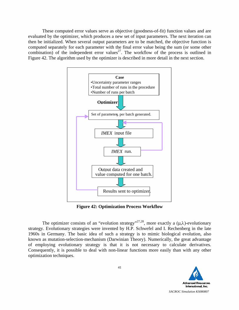
These computed error values serve as objective (goodness-of-fit) function values and are evaluated by the optimizer, which produces a new set of input parameters. The next iteration can then be initialized. When several output parameters are to be matched, the objective function is computed separately for each parameter with the final error value being the sum (or some other combination) of the independent error values27. The workflow of the process is outlined in Figure 42. The algorithm used by the optimizer is described in more detail in the next section.
Figure 42: Optimization Process Workflow
The optimizer consists of an “evolution strategy”27,28, more exactly a (µ,λ)-evolutionary
strategy. Evolutionary strategies were invented by H.P. Schwefel and I. Rechenberg in the late 1960s in Germany. The basic idea of such a strategy is to mimic biological evolution, also known as mutation-selection-mechanism (Darwinian Theory). Numerically, the great advantage of employing evolutionary strategy is that it is not necessary to calculate derivatives. Consequently, it is possible to deal with non-linear functions more easily than with any other optimization techniques.
Case • Uncertain parameters’ ranges • Total number of runs in the • Number of runs per
Optimizer
Set of parameter s
IMEX input file
IMEX run.
Output data created and value computed for one batch.
Results sent to optimizer.
per batch generated.
Case•Uncertainty parameter ranges•Total number of runs in the procedure•Number of runs per batch
SACROC Simulation KS080807
42
The algorithm is initialized with a set of λ individuals, where an individual represents a solution in the given search space. The optimizer can support the distribution of λ individuals in the search space completely arbitrarily or via initialization with a given start point. The latter can be used if an optimization will be based on a known good solution.
The λ individuals are then evaluated -- meaning in this particular case, that for each set of
individuals a complete set of simulation iterations are executed. Once completed, the objective value can be calculated as previously described. The next step in the optimization loop is the “selection” mechanism where the individuals are sorted according to their objective values. The population for the next generation is then created by taking the best µ individuals from the λ individuals (also called “comma-selection”).
In order to exchange information about the topology between the individuals, the next applied operator is the recombination operator. Usually two individuals from these µ are taken randomly to create a new individual. Here an “intermediate recombination” is used, i.e. for each dimension the average of the values of the two participating parent individuals is calculated. This is done until λ offspring are generated.
Since the recombination is responsible for large moves in the search space, the
subsequent “mutation” is applied to make smaller moves and hence to search more locally. The value of each individual’s dimension is mutated by adding a normal distributed term which is calculated based on the parameters of global sigma (σ) and local sigma (σi). These additional variables are called “step sizes” or “strategic variables” and belong to the individual’s gene type as the objective variables (input variables) do. Due to the normal distribution, smaller changes are more likely than greater changes. The σ, σi itself are also underlying a normal distributed variation. This means the step sizes change and should always be adapted to the current fitness landscape. This mechanism is called “self-adaptation”27,28
Although an evolutionary algorithm is a very general and robust optimization technique,
it is possible in each specific case to make the optimization more efficient and converge faster by applying known domain knowledge and good parameter settings.
6.2 Optimized Parameters
Some input parameters were unavailable for the study. Those parameters were varied during the history matching as were uncertain parameters. The porosity and permeability characterizations were developed in a grid that could work directly in the flow simulator3. Both the geostatistical characterizations and the reservoir flow simulations were conducted on the same Cartesian grid. Confidence in the porosity model developed with this grid definition was high, but it was suspected that the values of permeability populating the model grid-blocks could have been underestimated.
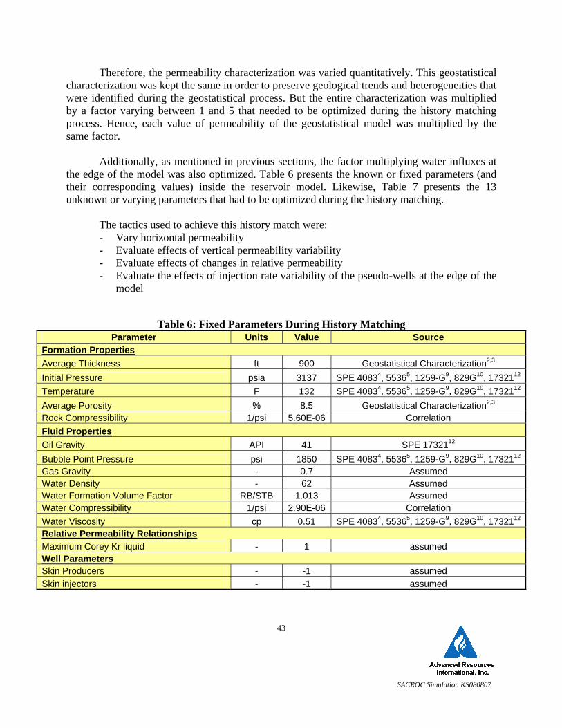
SACROC Simulation KS080807
43
Therefore, the permeability characterization was varied quantitatively. This geostatistical characterization was kept the same in order to preserve geological trends and heterogeneities that were identified during the geostatistical process. But the entire characterization was multiplied by a factor varying between 1 and 5 that needed to be optimized during the history matching process. Hence, each value of permeability of the geostatistical model was multiplied by the same factor.
Additionally, as mentioned in previous sections, the factor multiplying water influxes at
the edge of the model was also optimized. Table 6 presents the known or fixed parameters (and their corresponding values) inside the reservoir model. Likewise, Table 7 presents the 13 unknown or varying parameters that had to be optimized during the history matching.
The tactics used to achieve this history match were: - Vary horizontal permeability - Evaluate effects of vertical permeability variability - Evaluate effects of changes in relative permeability - Evaluate the effects of injection rate variability of the pseudo-wells at the edge of the
model
Table 6: Fixed Parameters During History Matching Parameter Units Value Source
Formation Properties Average Thickness ft 900 Geostatistical Characterization2,3 Initial Pressure psia 3137 SPE 40834, 55365, 1259-G9, 829G10, 1732112
Temperature F 132 SPE 40834, 55365, 1259-G9, 829G10, 1732112
Average Porosity % 8.5 Geostatistical Characterization2,3 Rock Compressibility 1/psi 5.60E-06 Correlation Fluid Properties Oil Gravity API 41 SPE 1732112 Bubble Point Pressure psi 1850 SPE 40834, 55365, 1259-G9, 829G10, 1732112
Gas Gravity - 0.7 Assumed Water Density - 62 Assumed Water Formation Volume Factor RB/STB 1.013 Assumed Water Compressibility 1/psi 2.90E-06 Correlation Water Viscosity cp 0.51 SPE 40834, 55365, 1259-G9, 829G10, 1732112
Relative Permeability Relationships Maximum Corey Kr liquid - 1 assumed Well Parameters Skin Producers - -1 assumed Skin injectors - -1 assumed
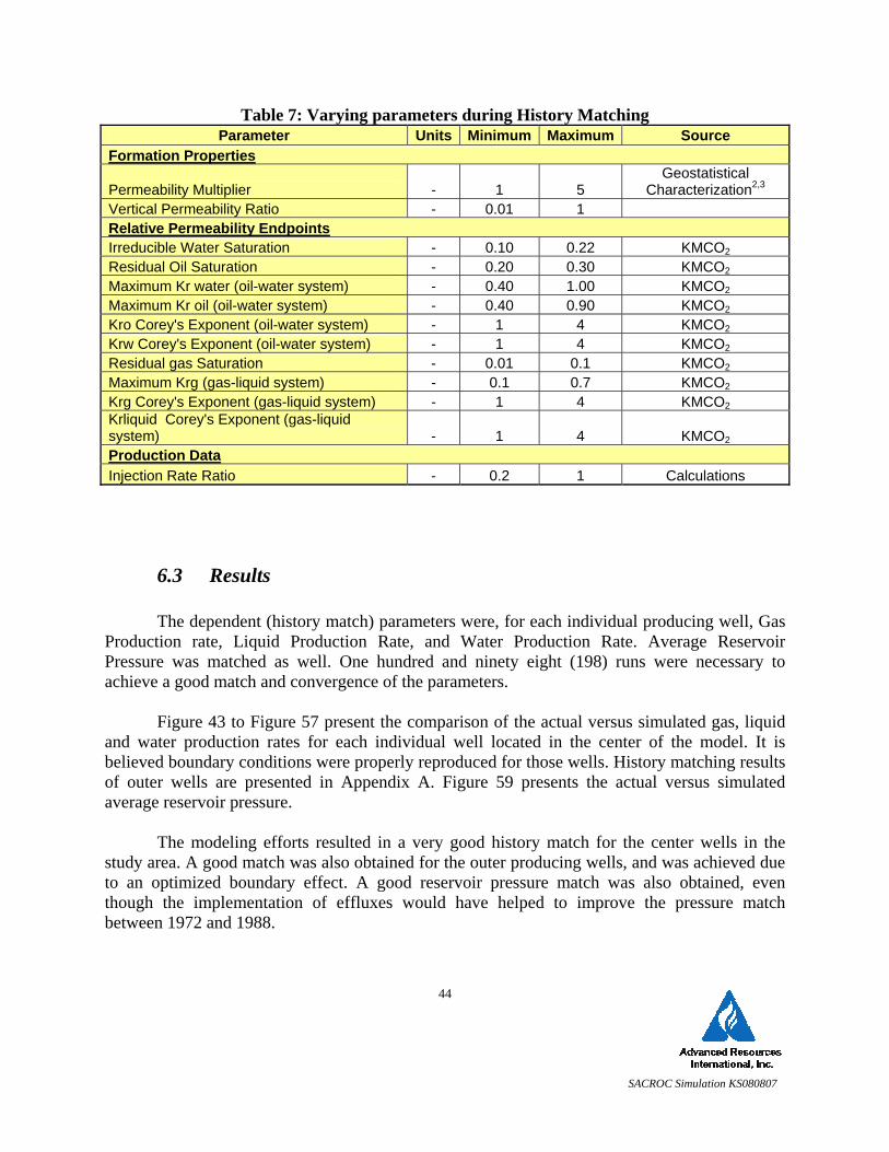
SACROC Simulation KS080807
44
Table 7: Varying parameters during History Matching Parameter Units Minimum Maximum Source
Formation Properties
Permeability Multiplier - 1 5 Geostatistical
Characterization2,3 Vertical Permeability Ratio - 0.01 1 Relative Permeability Endpoints Irreducible Water Saturation - 0.10 0.22 KMCO2 Residual Oil Saturation - 0.20 0.30 KMCO2 Maximum Kr water (oil-water system) - 0.40 1.00 KMCO2 Maximum Kr oil (oil-water system) - 0.40 0.90 KMCO2 Kro Corey's Exponent (oil-water system) - 1 4 KMCO2 Krw Corey's Exponent (oil-water system) - 1 4 KMCO2 Residual gas Saturation - 0.01 0.1 KMCO2 Maximum Krg (gas-liquid system) - 0.1 0.7 KMCO2 Krg Corey's Exponent (gas-liquid system) - 1 4 KMCO2 Krliquid Corey's Exponent (gas-liquid system) - 1 4 KMCO2 Production Data Injection Rate Ratio - 0.2 1 Calculations
6.3 Results
The dependent (history match) parameters were, for each individual producing well, Gas Production rate, Liquid Production Rate, and Water Production Rate. Average Reservoir Pressure was matched as well. One hundred and ninety eight (198) runs were necessary to achieve a good match and convergence of the parameters.
Figure 43 to Figure 57 present the comparison of the actual versus simulated gas, liquid
and water production rates for each individual well located in the center of the model. It is believed boundary conditions were properly reproduced for those wells. History matching results of outer wells are presented in Appendix A. Figure 59 presents the actual versus simulated average reservoir pressure.
The modeling efforts resulted in a very good history match for the center wells in the
study area. A good match was also obtained for the outer producing wells, and was achieved due to an optimized boundary effect. A good reservoir pressure match was also obtained, even though the implementation of effluxes would have helped to improve the pressure match between 1972 and 1988.
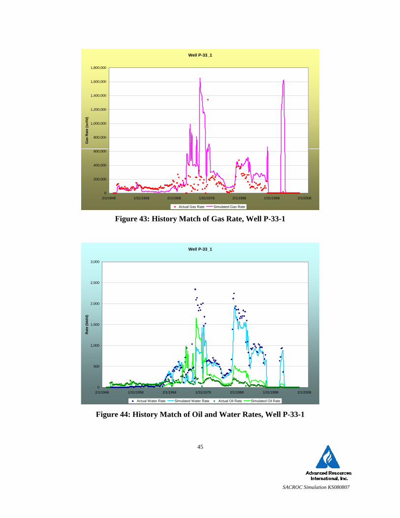
SACROC Simulation KS080807
45
Figure 43: History Match of Gas Rate, Well P-33-1
Figure 44: History Match of Oil and Water Rates, Well P-33-1
Well P-33_1
0
200,000
400,000
600,000
800,000
1,000,000
1,200,000
1,400,000
1,600,000
1,800,000
2/1/1948 1/31/1958 2/1/1968 1/31/1978 2/1/1988 1/31/1998 2/1/2008
Gas
Rat
e (s
cf/d
)
Actual Gas Rate Simulated Gas Rate
Well P-33_1
0
500
1,000
1,500
2,000
2,500
3,000
2/1/1948 1/31/1958 2/1/1968 1/31/1978 2/1/1988 1/31/1998 2/1/2008
Rat
e (b
bl/d
)
Actual Water Rate Simulated Water Rate Actual Oil Rate Simulated Oil Rate
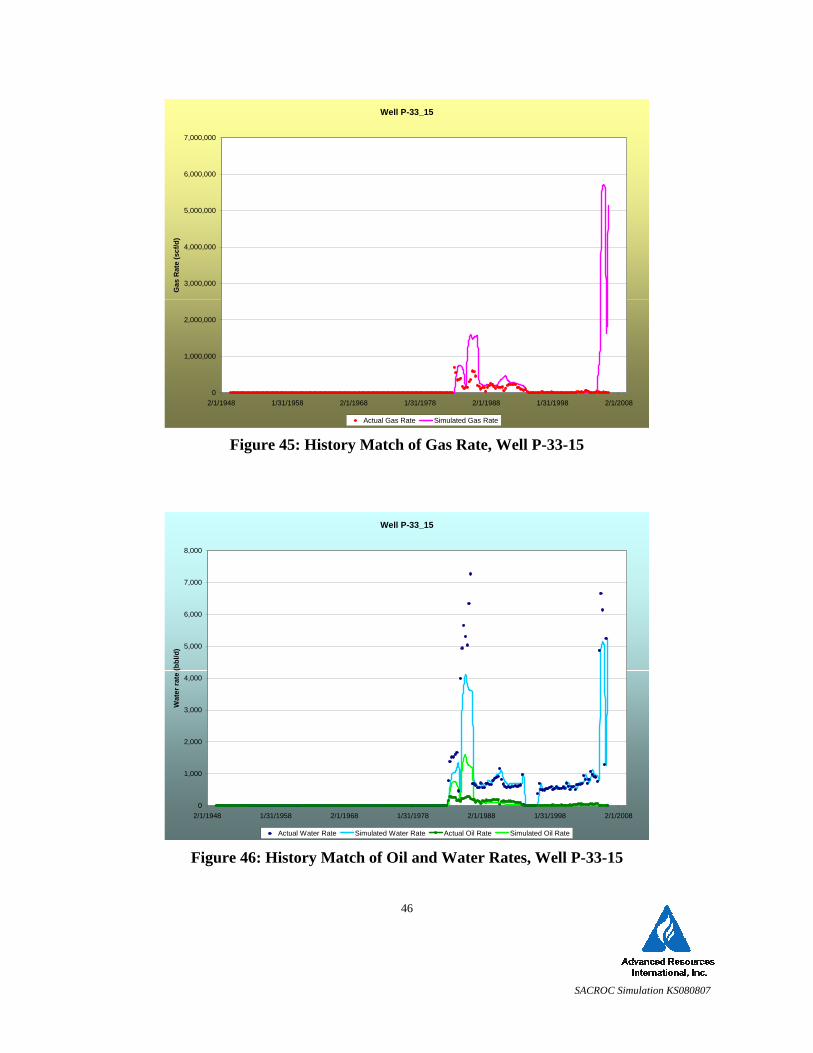
SACROC Simulation KS080807
46
Figure 45: History Match of Gas Rate, Well P-33-15
Figure 46: History Match of Oil and Water Rates, Well P-33-15
Well P-33_15
0
1,000,000
2,000,000
3,000,000
4,000,000
5,000,000
6,000,000
7,000,000
2/1/1948 1/31/1958 2/1/1968 1/31/1978 2/1/1988 1/31/1998 2/1/2008
Gas
Rat
e (s
cf/d
)
Actual Gas Rate Simulated Gas Rate
Well P-33_15
0
1,000
2,000
3,000
4,000
5,000
6,000
7,000
8,000
2/1/1948 1/31/1958 2/1/1968 1/31/1978 2/1/1988 1/31/1998 2/1/2008
Wat
er ra
te (b
bl/d
)
Actual Water Rate Simulated Water Rate Actual Oil Rate Simulated Oil Rate
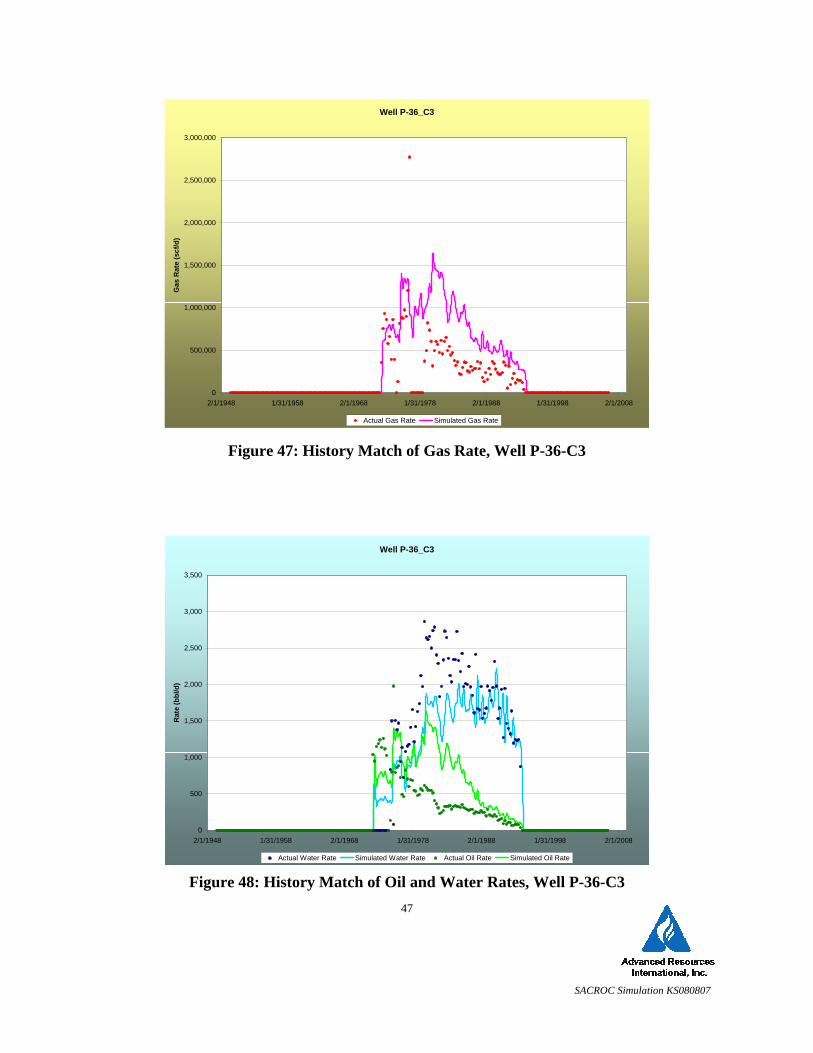
SACROC Simulation KS080807
47
Figure 47: History Match of Gas Rate, Well P-36-C3
Figure 48: History Match of Oil and Water Rates, Well P-36-C3
Well P-36_C3
0
500,000
1,000,000
1,500,000
2,000,000
2,500,000
3,000,000
2/1/1948 1/31/1958 2/1/1968 1/31/1978 2/1/1988 1/31/1998 2/1/2008
Gas
Rat
e (s
cf/d
)
Actual Gas Rate Simulated Gas Rate
Well P-36_C3
0
500
1,000
1,500
2,000
2,500
3,000
3,500
2/1/1948 1/31/1958 2/1/1968 1/31/1978 2/1/1988 1/31/1998 2/1/2008
Rat
e (b
bl/d
)
Actual Water Rate Simulated Water Rate Actual Oil Rate Simulated Oil Rate
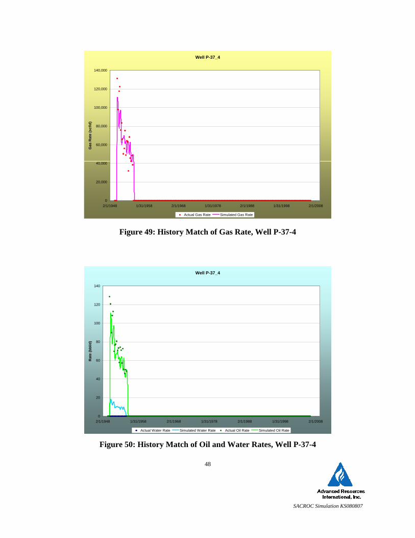
SACROC Simulation KS080807
48
Figure 49: History Match of Gas Rate, Well P-37-4
Figure 50: History Match of Oil and Water Rates, Well P-37-4
Well P-37_4
0
20,000
40,000
60,000
80,000
100,000
120,000
140,000
2/1/1948 1/31/1958 2/1/1968 1/31/1978 2/1/1988 1/31/1998 2/1/2008
Gas
Rat
e (s
cf/d
)
Actual Gas Rate Simulated Gas Rate
Well P-37_4
0
20
40
60
80
100
120
140
2/1/1948 1/31/1958 2/1/1968 1/31/1978 2/1/1988 1/31/1998 2/1/2008
Rat
e (b
bl/d
)
Actual Water Rate Simulated Water Rate Actual Oil Rate Simulated Oil Rate
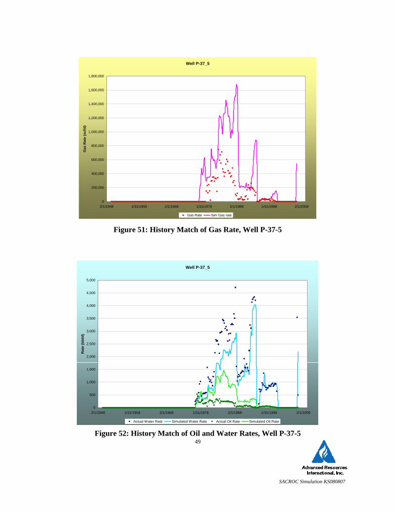
SACROC Simulation KS080807
49
Figure 51: History Match of Gas Rate, Well P-37-5
Figure 52: History Match of Oil and Water Rates, Well P-37-5
Well P-37_5
0
500
1,000
1,500
2,000
2,500
3,000
3,500
4,000
4,500
5,000
2/1/1948 1/31/1958 2/1/1968 1/31/1978 2/1/1988 1/31/1998 2/1/2008
Rat
e (b
bl/d
)
Actual Water Rate Simulated Water Rate Actual Oil Rate Simulated Oil Rate
Well P-37_5
0
200,000
400,000
600,000
800,000
1,000,000
1,200,000
1,400,000
1,600,000
1,800,000
2/1/1948 1/31/1958 2/1/1968 1/31/1978 2/1/1988 1/31/1998 2/1/2008
Gas
Rat
e (s
cf/d
)
Gas Rate Sim Gas rate
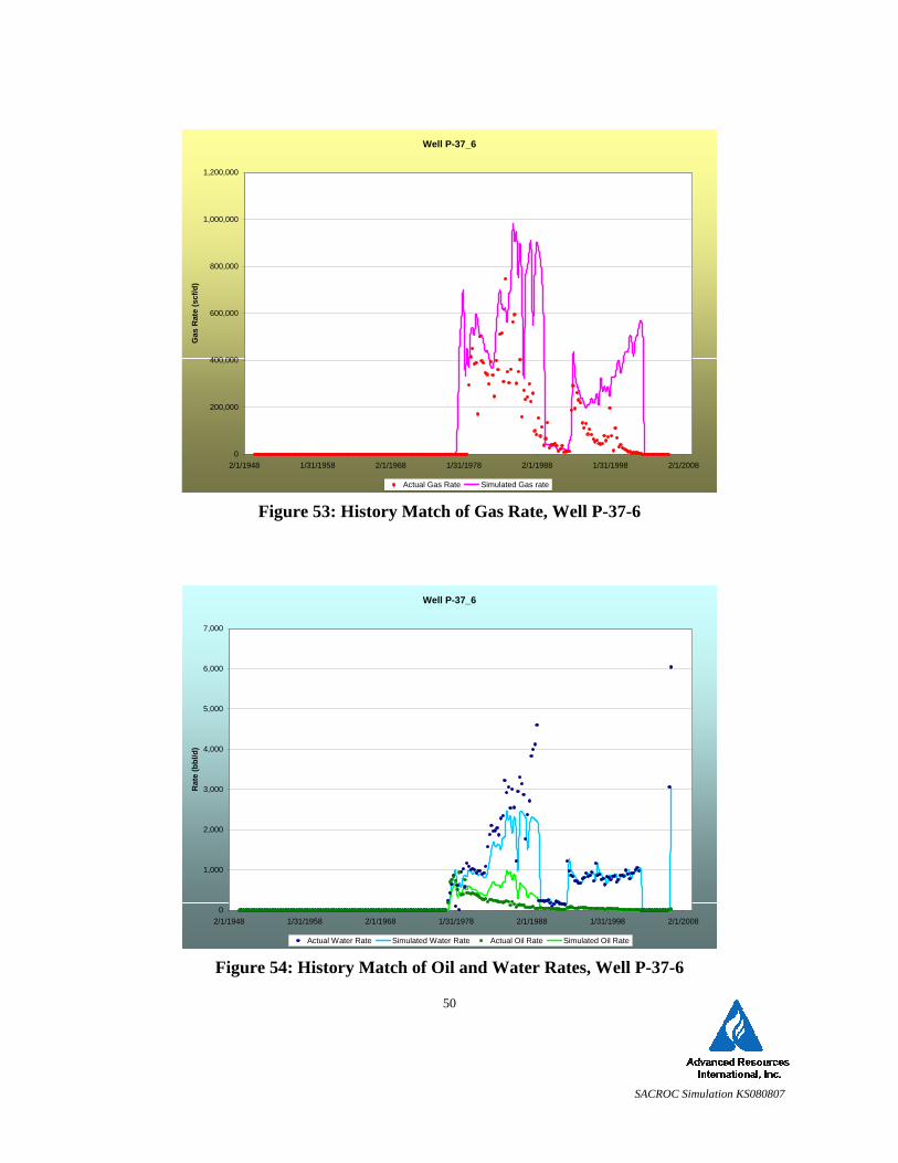
SACROC Simulation KS080807
50
Figure 53: History Match of Gas Rate, Well P-37-6
Figure 54: History Match of Oil and Water Rates, Well P-37-6
Well P-37_6
0
200,000
400,000
600,000
800,000
1,000,000
1,200,000
2/1/1948 1/31/1958 2/1/1968 1/31/1978 2/1/1988 1/31/1998 2/1/2008
Gas
Rat
e (s
cf/d
)
Actual Gas Rate Simulated Gas rate
Well P-37_6
0
1,000
2,000
3,000
4,000
5,000
6,000
7,000
2/1/1948 1/31/1958 2/1/1968 1/31/1978 2/1/1988 1/31/1998 2/1/2008
Rat
e (b
bl/d
)
Actual Water Rate Simulated Water Rate Actual Oil Rate Simulated Oil Rate

SACROC Simulation KS080807
51
Figure 55: History Match of Gas Rate, Well P-59-1
Figure 56: History Match of Oil and Water Rates, Well P-59-1
Well P-59_1
0
50,000
100,000
150,000
200,000
250,000
2/1/1948 1/31/1958 2/1/1968 1/31/1978 2/1/1988 1/31/1998 2/1/2008
Gas
Rat
e (s
cf/d
)
Actual Gas Rate Simulated Gas Rate
Well P-59_1
0
50
100
150
200
250
2/1/1948 1/31/1958 2/1/1968 1/31/1978 2/1/1988 1/31/1998 2/1/2008
Rat
e (b
bl/d
)
Actual Water Rate Simulated Water Rate Actual Oil Rate Simulated Oil Rate
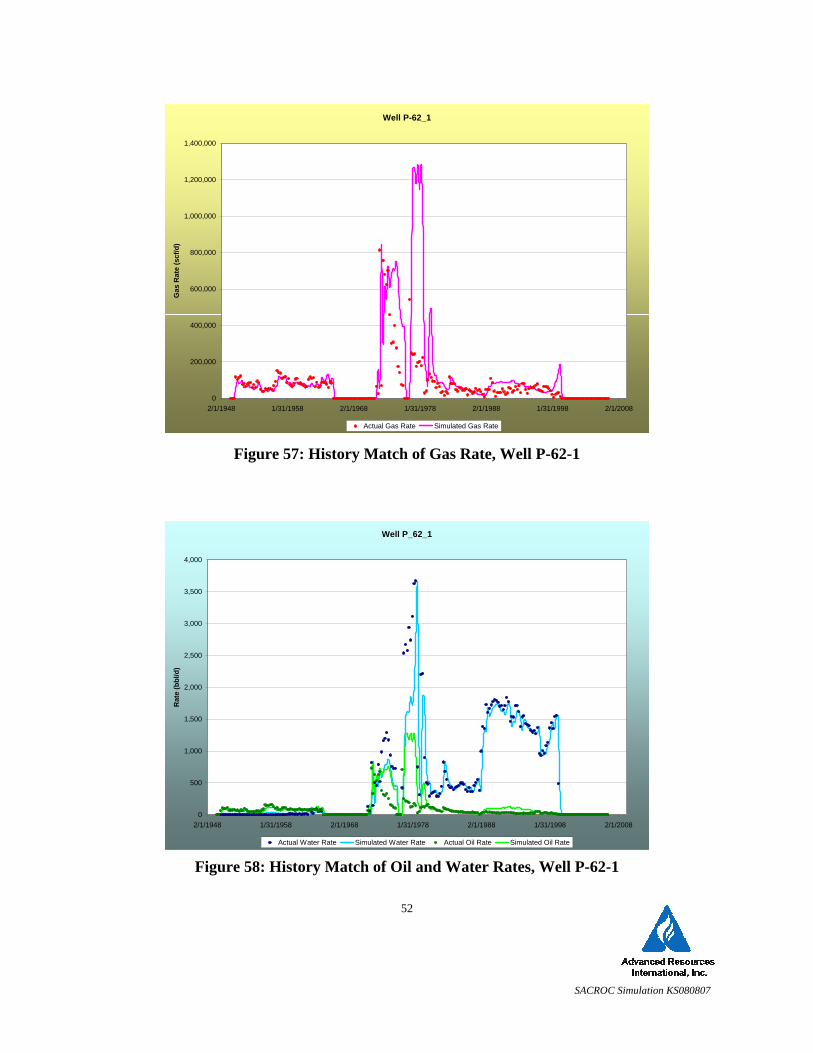
SACROC Simulation KS080807
52
Figure 57: History Match of Gas Rate, Well P-62-1
Figure 58: History Match of Oil and Water Rates, Well P-62-1
Well P-62_1
0
200,000
400,000
600,000
800,000
1,000,000
1,200,000
1,400,000
2/1/1948 1/31/1958 2/1/1968 1/31/1978 2/1/1988 1/31/1998 2/1/2008
Gas
Rat
e (s
cf/d
)
Actual Gas Rate Simulated Gas Rate
Well P_62_1
0
500
1,000
1,500
2,000
2,500
3,000
3,500
4,000
2/1/1948 1/31/1958 2/1/1968 1/31/1978 2/1/1988 1/31/1998 2/1/2008
Rat
e (b
bl/d
)
Actual Water Rate Simulated Water Rate Actual Oil Rate Simulated Oil Rate
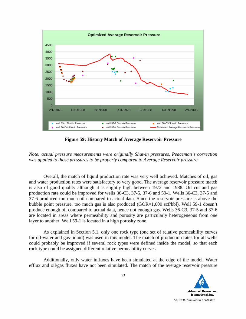
SACROC Simulation KS080807
53
Figure 59: History Match of Average Reservoir Pressure Note: actual pressure measurements were originally Shut-in pressures. Peaceman’s correction was applied to those pressures to be properly compared to Average Reservoir pressure.
Overall, the match of liquid production rate was very well achieved. Matches of oil, gas and water production rates were satisfactory to very good. The average reservoir pressure match is also of good quality although it is slightly high between 1972 and 1988. Oil cut and gas production rate could be improved for wells 36-C3, 37-5, 37-6 and 59-1. Wells 36-C3, 37-5 and 37-6 produced too much oil compared to actual data. Since the reservoir pressure is above the bubble point pressure, too much gas is also produced (GOR=1,000 scf/bbl). Well 59-1 doesn’t produce enough oil compared to actual data, hence not enough gas. Wells 36-C3, 37-5 and 37-6 are located in areas where permeability and porosity are particularly heterogeneous from one layer to another. Well 59-1 is located in a high porosity zone.
As explained in Section 5.1, only one rock type (one set of relative permeability curves
for oil-water and gas-liquid) was used in this model. The match of production rates for all wells could probably be improved if several rock types were defined inside the model, so that each rock type could be assigned different relative permeability curves.
Additionally, only water influxes have been simulated at the edge of the model. Water
efflux and oil/gas fluxes have not been simulated. The match of the average reservoir pressure
Optimized Average Reservoir Pressure
0
500
1000
1500
2000
2500
3000
3500
4000
4500
2/1/1948 1/31/1958 2/1/1968 1/31/1978 2/1/1988 1/31/1998 2/1/2008
well 33-1 Shut-In Pressure well 33-2 Shut-In Pressure well 36-C3 Shut-In Pressure
well 36-D4 Shut-In Pressure well 37-4 Shut-In Pressure Simulated Average Reservoir Pressure
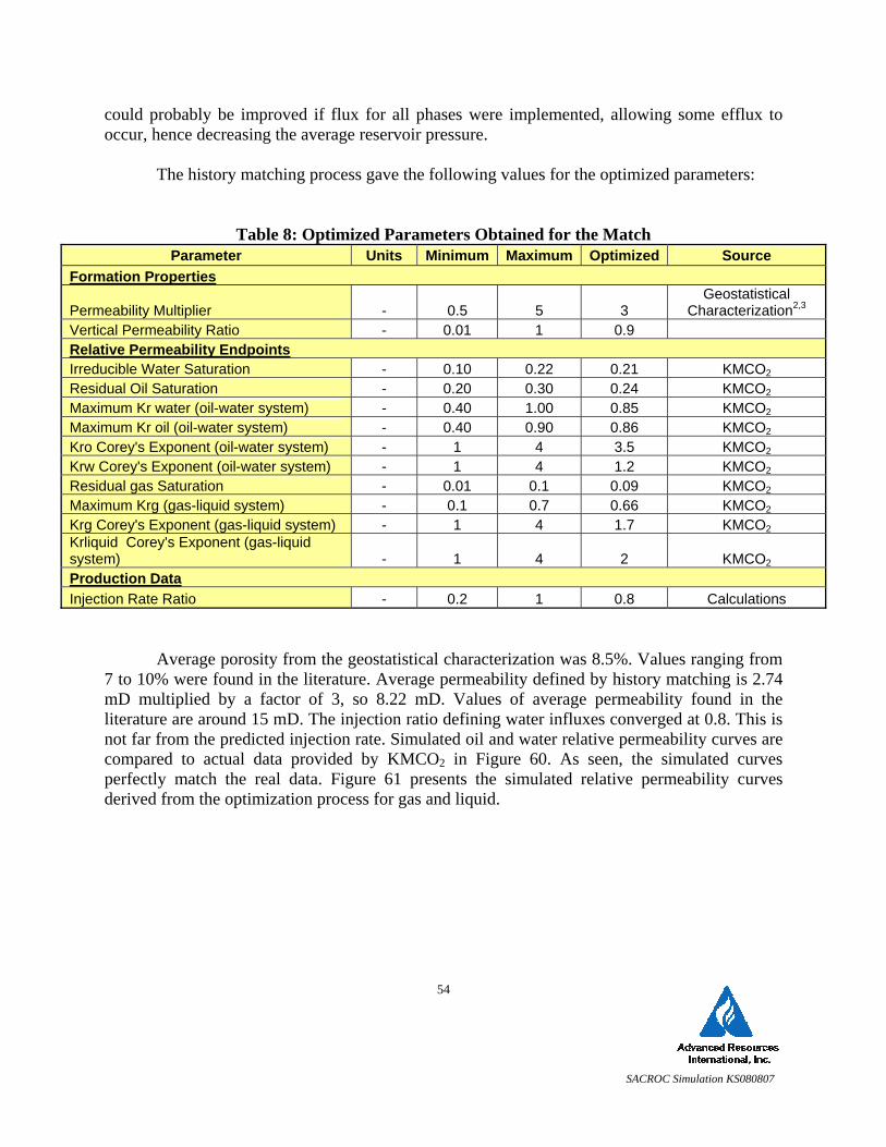
SACROC Simulation KS080807
54
could probably be improved if flux for all phases were implemented, allowing some efflux to occur, hence decreasing the average reservoir pressure.
The history matching process gave the following values for the optimized parameters:
Table 8: Optimized Parameters Obtained for the Match Parameter Units Minimum Maximum Optimized Source
Formation Properties
Permeability Multiplier - 0.5 5 3 Geostatistical
Characterization2,3 Vertical Permeability Ratio - 0.01 1 0.9 Relative Permeability Endpoints Irreducible Water Saturation - 0.10 0.22 0.21 KMCO2 Residual Oil Saturation - 0.20 0.30 0.24 KMCO2 Maximum Kr water (oil-water system) - 0.40 1.00 0.85 KMCO2 Maximum Kr oil (oil-water system) - 0.40 0.90 0.86 KMCO2 Kro Corey's Exponent (oil-water system) - 1 4 3.5 KMCO2 Krw Corey's Exponent (oil-water system) - 1 4 1.2 KMCO2 Residual gas Saturation - 0.01 0.1 0.09 KMCO2 Maximum Krg (gas-liquid system) - 0.1 0.7 0.66 KMCO2 Krg Corey's Exponent (gas-liquid system) - 1 4 1.7 KMCO2 Krliquid Corey's Exponent (gas-liquid system) - 1 4 2 KMCO2 Production Data Injection Rate Ratio - 0.2 1 0.8 Calculations
Average porosity from the geostatistical characterization was 8.5%. Values ranging from 7 to 10% were found in the literature. Average permeability defined by history matching is 2.74 mD multiplied by a factor of 3, so 8.22 mD. Values of average permeability found in the literature are around 15 mD. The injection ratio defining water influxes converged at 0.8. This is not far from the predicted injection rate. Simulated oil and water relative permeability curves are compared to actual data provided by KMCO2 in Figure 60. As seen, the simulated curves perfectly match the real data. Figure 61 presents the simulated relative permeability curves derived from the optimization process for gas and liquid.
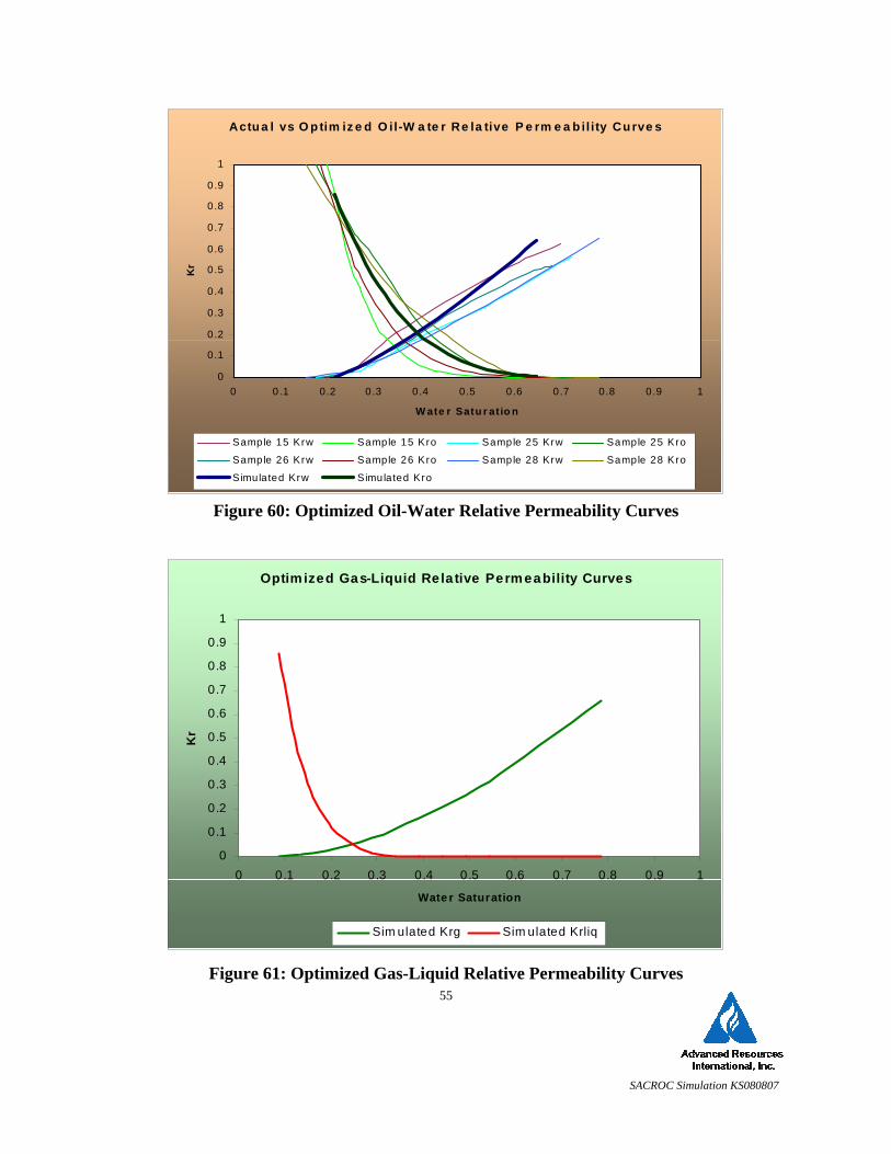
SACROC Simulation KS080807
55
Figure 60: Optimized Oil-Water Relative Permeability Curves
Figure 61: Optimized Gas-Liquid Relative Permeability Curves
Actu a l vs O p tim iz e d O il-W a te r Re la tive P e rm e a b il ity Cu rve s
0
0.1
0.2
0.3
0.4
0.5
0.6
0.7
0.8
0.9
1
0 0.1 0.2 0.3 0.4 0.5 0.6 0.7 0.8 0.9 1
W ate r Satu r at io n
Kr
Sample 15 Krw Sample 15 Kro Sample 25 Krw Sample 25 Kro
Sample 26 Krw Sample 26 Kro Sample 28 Krw Sample 28 Kro
Simulated Krw Simulated Kro
Optimized Gas-Liquid Rela tive Permeability Curves
0
0.1
0.2
0.3
0.4
0.5
0.6
0.7
0.8
0.9
1
0 0.1 0.2 0.3 0.4 0.5 0.6 0.7 0.8 0.9 1
Wate r Saturation
Kr
Sim ulated Krg Sim ulated Krliq
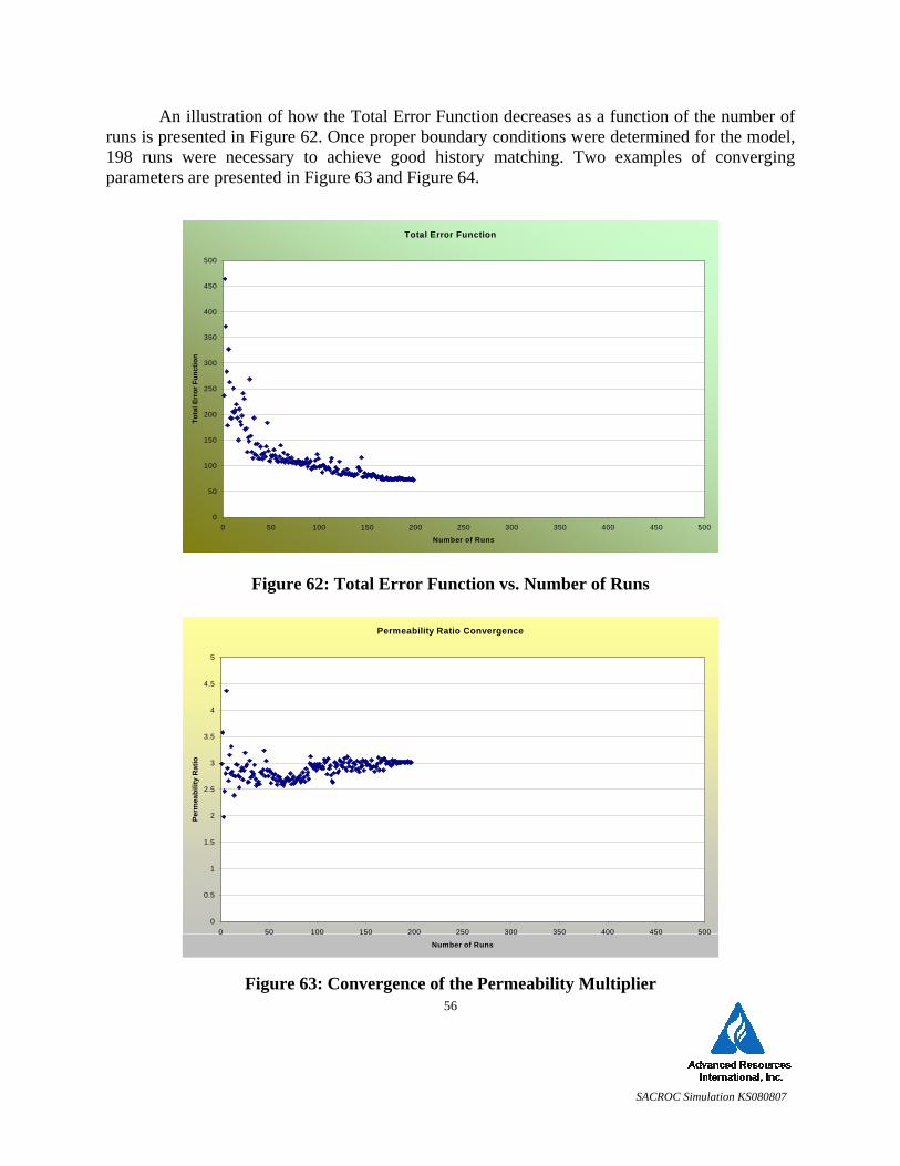
SACROC Simulation KS080807
56
An illustration of how the Total Error Function decreases as a function of the number of runs is presented in Figure 62. Once proper boundary conditions were determined for the model, 198 runs were necessary to achieve good history matching. Two examples of converging parameters are presented in Figure 63 and Figure 64.
Figure 62: Total Error Function vs. Number of Runs
Figure 63: Convergence of the Permeability Multiplier
Total Error Function
0
50
100
150
200
250
300
350
400
450
500
0 50 100 150 200 250 300 350 400 450 500
Number of Runs
Tota
l Err
or F
unct
ion
Permeability Ratio Convergence
0
0.5
1
1.5
2
2.5
3
3.5
4
4.5
5
0 50 100 150 200 250 300 350 400 450 500
Number of Runs
Perm
eabi
lity
Rat
io
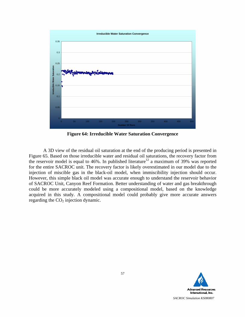
SACROC Simulation KS080807
57
Figure 64: Irreducible Water Saturation Convergence
A 3D view of the residual oil saturation at the end of the producing period is presented in Figure 65. Based on those irreducible water and residual oil saturations, the recovery factor from the reservoir model is equal to 46%. In published literature12 a maximum of 39% was reported for the entire SACROC unit. The recovery factor is likely overestimated in our model due to the injection of miscible gas in the black-oil model, when immiscibility injection should occur. However, this simple black oil model was accurate enough to understand the reservoir behavior of SACROC Unit, Canyon Reef Formation. Better understanding of water and gas breakthrough could be more accurately modeled using a compositional model, based on the knowledge acquired in this study. A compositional model could probably give more accurate answers regarding the CO2 injection dynamic.
Irreducible Water Saturation Convergence
0
0.05
0.1
0.15
0.2
0.25
0.3
0.35
0 50 100 150 200 250 300 350 400 450 500
Number Of Runs
Irred
ucib
le W
ater
Sat
urat
ion
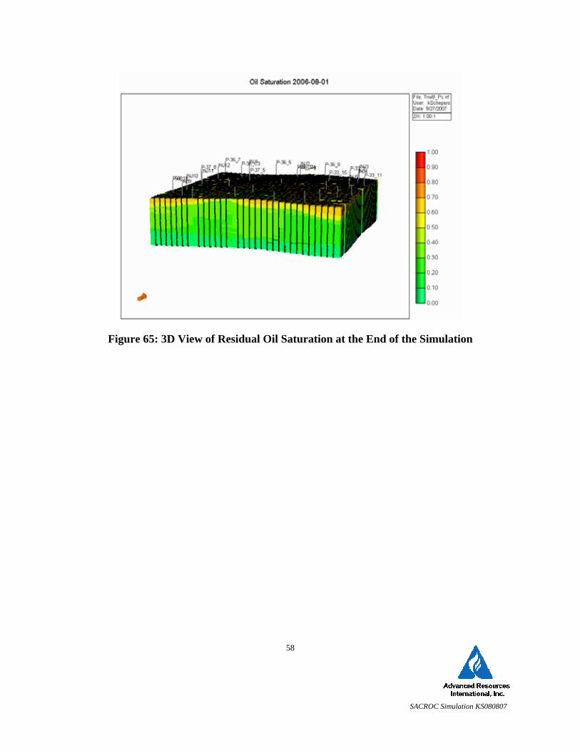
SACROC Simulation KS080807
58
Figure 65: 3D View of Residual Oil Saturation at the End of the Simulation
SACROC Simulation KS080807
59
7.0 Conclusions
1. An assisted history match was achieved using a global optimization method (evolutionary algorithms). This history match, in which several results were produced, was based on the matching of oil, gas and water production rates, and the average reservoir pressure. The match was accomplished by manipulating 13 uncertain design parameters which included two formation properties, other ten variables related with the corresponding relative permeability curves, and one variable linked to the reservoir production.
2. Evolutionary algorithms are widely accepted as robust optimization methodologies that can handle a large
amount of input design parameters. And, in this work, they were successfully applied for history matching complex reservoir performance drivers thanks to their capabilities to explore an enormous range of parameter combinations and produce lots of results related to the reservoir performance.
3. History match results confirmed that the 3D reservoir models of porosity and permeability constructed
applying the combined reservoir characterization approach (advanced pattern recognition techniques and geostatistical algorithms) were legitimate representations of the spatial distribution of these parameters in the reservoir.
4. The assisted history match procedure confirmed initial assumptions that the developed porosity model was
highly trustworthy, whereas the permeability model, despite of capturing correctly geological trends and heterogeneities of Canyon Reef reservoir (SACROC field) presented slightly underestimated values.
5. The modeling efforts resulted in a very good history match for the center wells in the study area. A good
match was also achieved for the outer producing wells and the average reservoir pressure. These achievements were thanks to the setting up of proper boundary conditions that described the flow behavior at the boundary of the analyzed region.
6. Overall, the match of liquid production rate was very well achieved. Matches of oil, gas and water
production rates were from satisfactory to very good. The average reservoir pressure match was also of good quality although slightly high between years 1972 and 1988.
7. Application of several techniques for estimating water influxes allowed the definition of proper boundary
conditions for the simulation model. The adopted influxes techniques were very important to achieve very good history match results.
8. The implementation of twelve pseudo-injectors at the boundaries of the study area reproduced accurately
water influxes at the edge of the model. The use of a multiplicative factor for water influxes at the edge of the model was determinant in this process. This factor, varied between 0.2 and 1, converged at 0.8 which was close to calculated injection rates using differential water volume technique (Method 2).
9. The simple black oil model developed here was sufficient to capture the reservoir behavior of SACROC
Unit, Canyon Reef Formation:
• Simulated oil-water relative permeability curves match perfectly actual core measurements • The recovery factor from the simulated reservoir model is equal to 46%; a maximum of 39% was
mentioned in literature.

SACROC Simulation KS080807
60
10. The recovery factor was probably overestimated due to the injection of miscible gas in our black-oil model, when immiscibility injection should have occurred. Better understanding of water and gas breakthrough could be more accurately modeled using a compositional model.
11. Based on the knowledge acquired in this study, most of the discrepancies reported here could be alleviated
or completely removed with the use of a compositional model, and the extension of the reservoir model to a larger drainage area.
12. The addition of optimization methods (for assisted history matching) to the combined soft-
computing/geostatistical approach (utilized for reservoir characterization purposes) constitutes a powerful triad of mathematical techniques ideally suited for addressing reservoir integrated studies, with the capacity of facing these complex tasks more rapidly and efficiently than using traditional methodologies.
SACROC Simulation KS080807
61
8.0 References
1. Reeves, S.R., Mohaghegh, S.D., Fairborn, J.W., and Luca, G.; “Feasibility Assessment of a New Approach for Integrating Multiscale Data for High-Resolution Reservoir Characterization”, SPE 77795, presented at the SPE Annual Technical Conference and Exhibition, San Antonio, Texas, September 29 - October 2, 2002.
2. González, R.J., Reeves, S.R., and Eslinger, E.; “Predicting Porosity and Permeability for the Canyon Formation, SACROC Unit (Kelly-Snyder Field), Using the Geologic Analysis via Maximum Likelihood System”, Topical Report prepared for U. S. Department of Energy, Contract Number DE-FC26-04NT15514, September, 2007.
3. González, R.J., Reeves, S.R., and Eslinger, E.; “Geostatistical Reservoir Characterization of the Canyon Formation, SACROC Unit, Permain Basin”, Topical Report for U. S. Department of Energy, Contract Number DE-FC26-04NT15514, September, 2007.
4. Dicharry, R.M., Perryman, T.L., Ronquille, J.D.; “Evaluation and Design of a CO2 Miscible Flood Project – SACROC Unit, Kelly-Snyder Field”, SPE 4083, prepared for the Journal of Petroleum Technology, pg. 1309 - 1318, November, 1973.
5. Brummett, W.M., Jr., Emanuel, A.S., Ronquille, J.D.; “Reservoir Description by Simulation at SACROC – A Case History”, SPE 5536, prepared for the Journal of Petroleum Technology, pg. 1241 – 1255, October, 1976.
6. Reeves, S.R.; “Demonstration of a Novel, Integrated, Multi-Scale Procedure for High-Resolution 3D Reservoir Characterization and Improved CO2-EOR/Sequestration Management, SACROC Unit”, prepared for U. S. Department of Energy, Solicitation Number DE-PS26-04NT15450-2C, February 10, 2004.
7. Hawkins, J.T., Benvegnu, A.J., Wingate, T.P., McKamie, J.D., Pickard, C.D., Altum, J.T.; “SACROC Unit CO2 Flood: Multidisciplinary Team Improves Reservoir Management and Decreases Operating Costs”, SPE 35359, presented at the 1996 SPE/DOE Symposium on Improved Oil Recovery, Tulsa, OK, April 21-24, 1996.
8. Remy, N.: “SGEMS: The Stanford Geostatistical Earth Modeling Software. User’s Manual”, http://sgems.sourceforge.net/doc/sgems_manual.pdf, May 2004.
9. Allen, H.H., Thomas, J.B.; “Pressure Maintenance in SACROC Unit Operations”, SPE 1259-G, presented at the Permian Basin Section Oil Recovery Conference, Midland, TX, May 7-8, 1959.
10. Allen, H.H., LaRue, C.R.; “SACROC Unit Operations”, SPE 829-G, presented at Permian Basin Oil Recovery Conference, Midland, TX, April 18-19, 1957.
11. Graue, D. J., Blevins, T.R.; “SACROC Tertiary CO2 Pilot Project”, SPE 7090, presented at the Fifth Symposium on Improved Methods for Oil Recovery of the Society of Petroleum Engineers of AIME, Tulsa, OK, April 16-19, 1978.
12. Langston, M.V., Hoadley, S.F., Young, D.N.; “Definitive CO2 Flooding Response in the SACROC Unit”, SPE 17321, prepared for the SPE/DOE Enhanced Oil Recovery Symposium, Tulsa, OK, April 17-20, 1988.
13. Kane, A.V.; “Performance Review of a Large-Scale CO2-WAG Enhanced Recovery Project, SACROC Unit, Kelly-Snyder Field”, SPE 7091, presented at the SPE/AIME
SACROC Simulation KS080807
62
Fifth Symposium on Improved Methods for Oil Recovery, Tulsa, OK, April 16-19, 1978.
14. “IMEX. Advanced Oil/Gas Reservoir Simulator. 2007 User’s Guide”, Computer Modelling Group Ltd., 2007.
15. Ramey, H.J. Jr.; “Rapid Methods for Estimating Reservoir Compressibilities,” JPT (April 1964) 447; Trans., AIME, 231.
16. McCain, W.D. Jr; “Reservoir-Fluid Property Correlations - State of the Art”, SPERE (May 1991) 266.
17. Standing, M.B. and Katz, D.L.; “Density of Natural Gases”, Trans. AIME (1942) 146, 140-149.
18. Dodson C.R. and Standing, M.B.; “Pressure, Volume, Temperature and Solubility Relations for Natural Gas-Water Mixtures”, Drill. & Prod. Prac. (1944) 173-179.
19. Earlougher, R.C., Jr.; “Advances in Well Test Analysis”, SPE Monograph Series, SPE, Richardson, Texas (1977) 5.
20. Rowe, A.M. Jr. and Chou, J.C.S.; “Pressure-Volume-Temperature-Concentration Relation of Aqueous NaCl Solutions,” J. Chem. Eng. Data (1970), 15, 61.
21. Matthews, C.S. and Russell, D.G.; “Pressure Buildup and Flow Tests in Wells”, Monograph Series, SPE, Dallas (1967) 1, Appendix G.
22. Standing, M.B.; “Volumetric and Phase Behavior of Oil Field Hydrocarbon Systems”, SPE, Richardson, TX, 1981.
23. Beggs, H.D. and Robinson J.R.; “Estimating the Viscosity of Crude Oil Systems”, J. Pet. Tech. (Sept. 1975) 1140-41.
24. Holtz, M.H., Smith, R.C., McPherson, B. and Han, W.C.; “Subsurface Site Characterization Methodology; Example from Pennsylvanian Carbonate Reef, West Texas”, prepared for DOE Southwest Partnership Pilot at SACROC and Claytonville oil field sites, February 16, 2006.
25. Carr, N.L., Kobayashi, R., and Burrows, D.B.; “Viscosity of the Hydrocarbon Gases Under Pressure,” Trans., AIME (1954) 201, 264-78.
26. Van Everdingen, A.F., Timmerman, E.H., and McMahon, J.J.; “Application of the Material Balance Equation to a Partial Water-Drive Reservoir”, Trans., AIME (1953) 198, 51-60.
27. Oudinot, A., Sultana, A., Gonzalez, R.J., Reeves, S.R., and Wörmann, M.; Development of Optimized History-Matched Models for Coalbed Methane Reservoirs.
28. Baeck, T., Fogel, D.B., Michalewicz, Z.; “Handbook of Evolutionary Computation”; Oxford University Press, New York, Oxford, 1997.
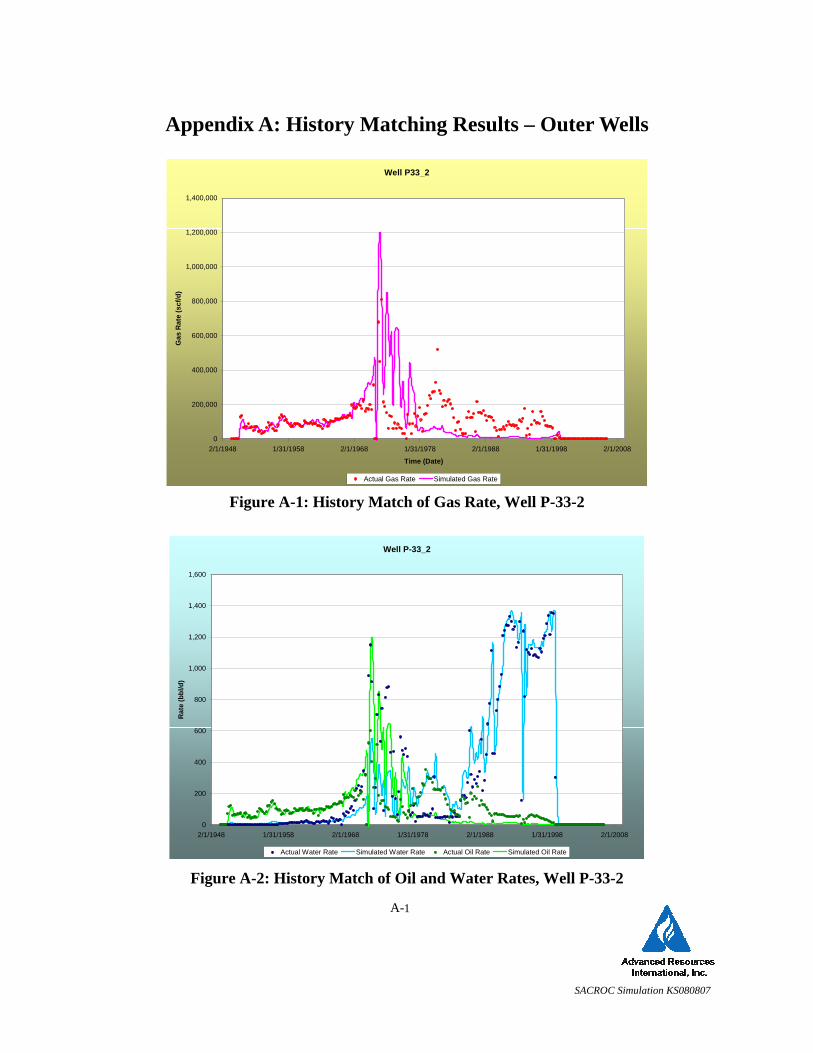
SACROC Simulation KS080807
1
Appendix A: History Matching Results – Outer Wells
Figure A-1: History Match of Gas Rate, Well P-33-2
Figure A-2: History Match of Oil and Water Rates, Well P-33-2
A-
Well P-33_2
0
200
400
600
800
1,000
1,200
1,400
1,600
2/1/1948 1/31/1958 2/1/1968 1/31/1978 2/1/1988 1/31/1998 2/1/2008
Rat
e (b
bl/d
)
Actual Water Rate Simulated Water Rate Actual Oil Rate Simulated Oil Rate
Well P33_2
0
200,000
400,000
600,000
800,000
1,000,000
1,200,000
1,400,000
2/1/1948 1/31/1958 2/1/1968 1/31/1978 2/1/1988 1/31/1998 2/1/2008
Time (Date)
Gas
Rat
e (s
cf/d
)
Actual Gas Rate Simulated Gas Rate
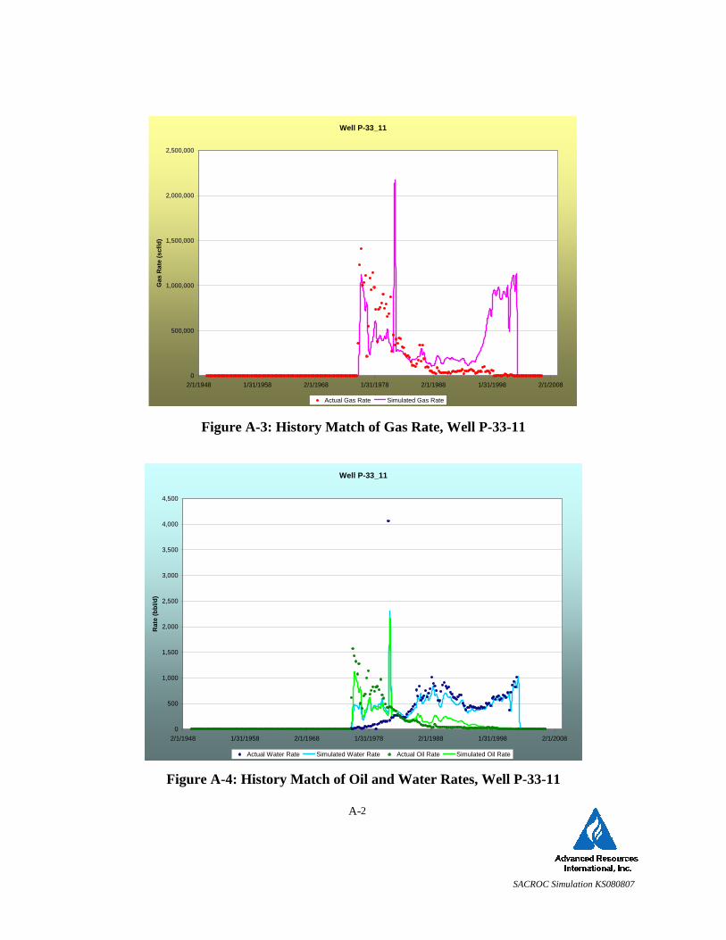
SACROC Simulation KS080807
2
Figure A-3: History Match of Gas Rate, Well P-33-11
Figure A-4: History Match of Oil and Water Rates, Well P-33-11
A-
Well P-33_11
0
500
1,000
1,500
2,000
2,500
3,000
3,500
4,000
4,500
2/1/1948 1/31/1958 2/1/1968 1/31/1978 2/1/1988 1/31/1998 2/1/2008
Rat
e (b
bl/d
)
Actual Water Rate Simulated Water Rate Actual Oil Rate Simulated Oil Rate
Well P-33_11
0
500,000
1,000,000
1,500,000
2,000,000
2,500,000
2/1/1948 1/31/1958 2/1/1968 1/31/1978 2/1/1988 1/31/1998 2/1/2008
Gas
Rat
e (s
cf/d
)
Actual Gas Rate Simulated Gas Rate
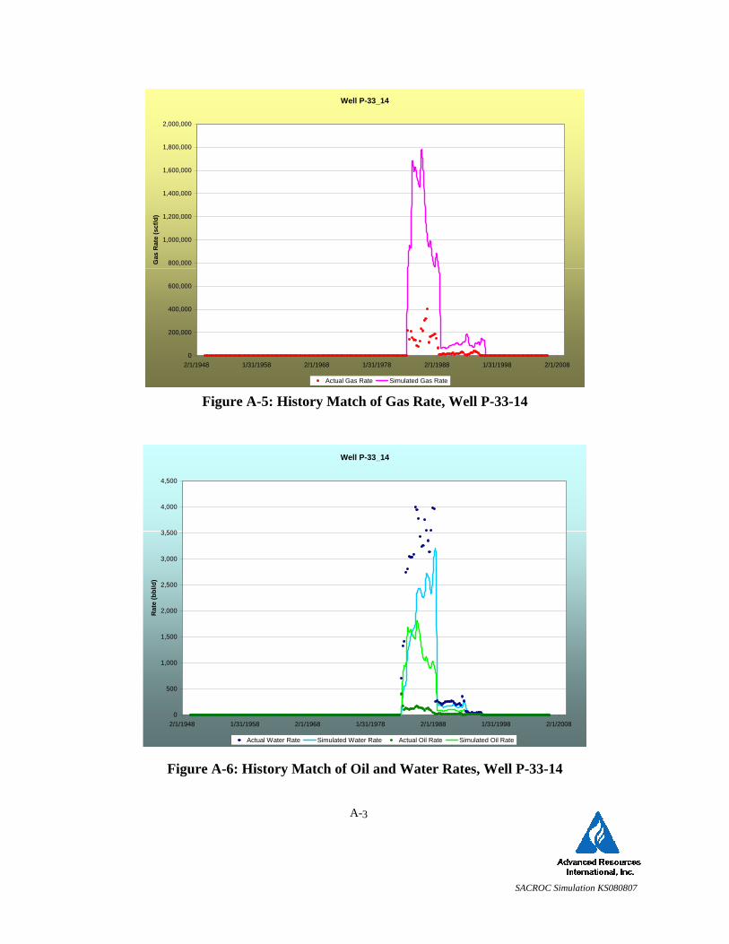
SACROC Simulation KS080807
3
Figure A-5: History Match of Gas Rate, Well P-33-14
Figure A-6: History Match of Oil and Water Rates, Well P-33-14
A-
Well P-33_14
0
200,000
400,000
600,000
800,000
1,000,000
1,200,000
1,400,000
1,600,000
1,800,000
2,000,000
2/1/1948 1/31/1958 2/1/1968 1/31/1978 2/1/1988 1/31/1998 2/1/2008
Gas
Rat
e (s
cf/d
)
Actual Gas Rate Simulated Gas Rate
Well P-33_14
0
500
1,000
1,500
2,000
2,500
3,000
3,500
4,000
4,500
2/1/1948 1/31/1958 2/1/1968 1/31/1978 2/1/1988 1/31/1998 2/1/2008
Rat
e (b
bl/d
)
Actual Water Rate Simulated Water Rate Actual Oil Rate Simulated Oil Rate
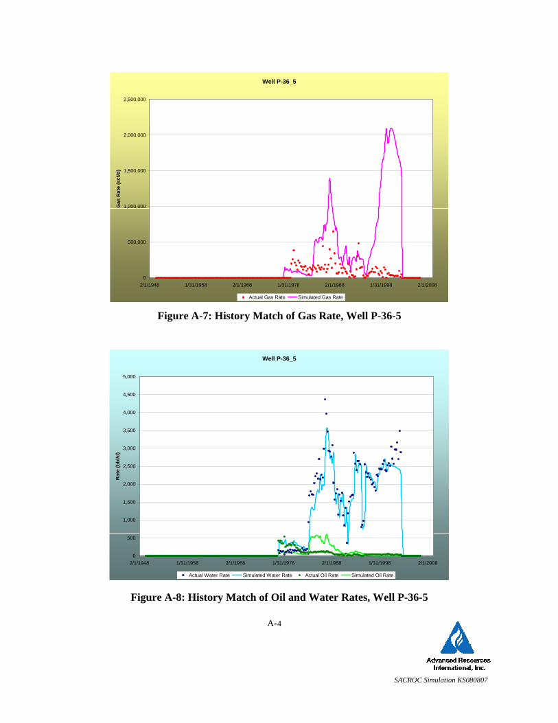
SACROC Simulation KS080807
4
Figure A-7: History Match of Gas Rate, Well P-36-5
Figure A-8: History Match of Oil and Water Rates, Well P-36-5
A-
Well P-36_5
0
500,000
1,000,000
1,500,000
2,000,000
2,500,000
2/1/1948 1/31/1958 2/1/1968 1/31/1978 2/1/1988 1/31/1998 2/1/2008
Gas
Rat
e (s
cf/d
)
Actual Gas Rate Simulated Gas Rate
Well P-36_5
0
500
1,000
1,500
2,000
2,500
3,000
3,500
4,000
4,500
5,000
2/1/1948 1/31/1958 2/1/1968 1/31/1978 2/1/1988 1/31/1998 2/1/2008
Rat
e (b
bl/d
)
Actual Water Rate Simulated Water Rate Actual Oil Rate Simulated Oil Rate
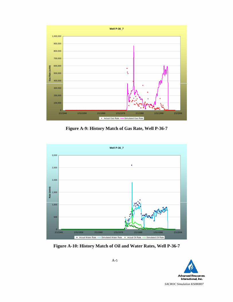
SACROC Simulation KS080807
5
Figure A-9: History Match of Gas Rate, Well P-36-7
Figure A-10: History Match of Oil and Water Rates, Well P-36-7
A-
Well P-36_7
0
100,000
200,000
300,000
400,000
500,000
600,000
700,000
800,000
900,000
1,000,000
2/1/1948 1/31/1958 2/1/1968 1/31/1978 2/1/1988 1/31/1998 2/1/2008
Gas
Rat
e (s
cf/d
)
Actual Gas Rate Simulated Gas Rate
Well P-36_7
0
500
1,000
1,500
2,000
2,500
3,000
2/1/1948 1/31/1958 2/1/1968 1/31/1978 2/1/1988 1/31/1998 2/1/2008
Rat
e (b
bl/d
)
Actual Water Rate Simulated Water Rate Actual Oil Rate Simulated Oil Rate
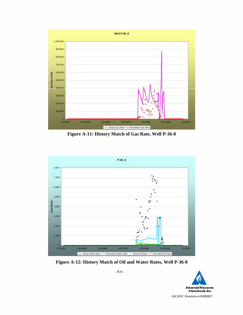
SACROC Simulation KS080807
6
Figure A-11: History Match of Gas Rate, Well P-36-8
Figure A-12: History Match of Oil and Water Rates, Well P-36-8
A-
Well P-36_8
0
100,000
200,000
300,000
400,000
500,000
600,000
700,000
800,000
900,000
1,000,000
2/1/1948 1/31/1958 2/1/1968 1/31/1978 2/1/1988 1/31/1998 2/1/2008
Gas
Rat
e (s
cf/d
)
Actual Gas Rate Simulated Gas Rate
P-36_8
0
1,000
2,000
3,000
4,000
5,000
6,000
7,000
8,000
2/1/1948 1/31/1958 2/1/1968 1/31/1978 2/1/1988 1/31/1998 2/1/2008
Rat
e (b
bl/d
)
Actual Water Rate Simulated Water Rate Actual Oil Rate Simulated Oil Rate
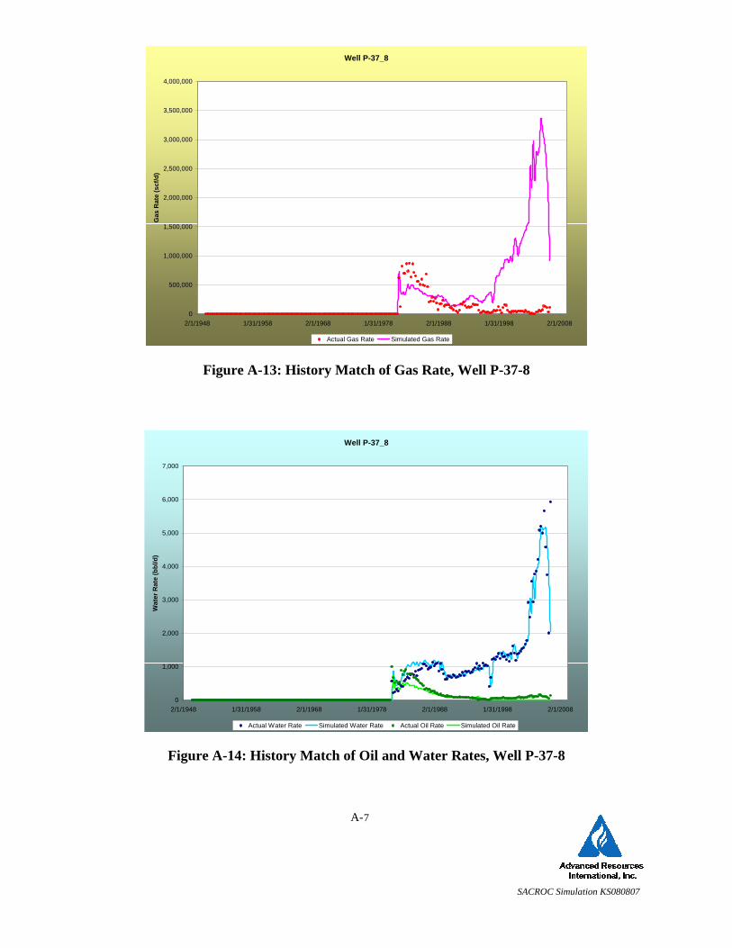
SACROC Simulation KS080807
7
Figure A-13: History Match of Gas Rate, Well P-37-8
Figure A-14: History Match of Oil and Water Rates, Well P-37-8
A-
Well P-37_8
0
500,000
1,000,000
1,500,000
2,000,000
2,500,000
3,000,000
3,500,000
4,000,000
2/1/1948 1/31/1958 2/1/1968 1/31/1978 2/1/1988 1/31/1998 2/1/2008
Gas
Rat
e (s
cf/d
)
Actual Gas Rate Simulated Gas Rate
Well P-37_8
0
1,000
2,000
3,000
4,000
5,000
6,000
7,000
2/1/1948 1/31/1958 2/1/1968 1/31/1978 2/1/1988 1/31/1998 2/1/2008
Wat
er R
ate
(bbl
/d)
Actual Water Rate Simulated Water Rate Actual Oil Rate Simulated Oil Rate
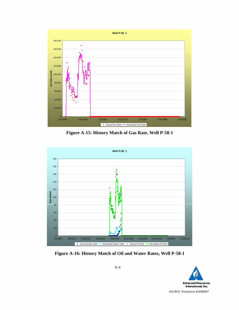
SACROC Simulation KS080807
8
Figure A-15: History Match of Gas Rate, Well P-58-1
Figure A-16: History Match of Oil and Water Rates, Well P-58-1
A-
Well P-58_1
0
20
40
60
80
100
120
140
160
180
200
1/0/1900 9/8/1913 5/18/1927 1/24/1941 10/3/1954 6/11/1968 2/18/1982 10/28/1995 7/6/2009 3/15/2023
Rat
e (b
bl/d
)
Actual Water Rate Simulated Water Rate Actual Oil Rate Simulated Oil Rate
Well P-58_1
0
20,000
40,000
60,000
80,000
100,000
120,000
140,000
160,000
180,000
2/1/1948 1/31/1958 2/1/1968 1/31/1978 2/1/1988 1/31/1998 2/1/2008
Gas
Rat
e (s
cf/d
)
Actual Gas Rate Simulated Gas Rate