Optimizing Glide-Flight Paths

Bard College Bard College

Bard Digital Commons Bard Digital Commons

Senior Projects Spring 2019 Bard Undergraduate Senior Projects

Spring 2019

Optimizing Glide-Flight Paths Optimizing Glide-Flight Paths

Rory Cveta O'Daly Maglich Bard College, [email protected]

Follow this and additional works at: https://digitalcommons.bard.edu/senproj_s2019

Part of the Fluid Dynamics Commons, and the Other Physics Commons

This work is licensed under a Creative Commons Attribution-Noncommercial-No Derivative Works 4.0 License.

Recommended Citation Recommended Citation Maglich, Rory Cveta O'Daly, "Optimizing Glide-Flight Paths" (2019). Senior Projects Spring 2019. 113. https://digitalcommons.bard.edu/senproj_s2019/113

This Open Access work is protected by copyright and/or related rights. It has been provided to you by Bard College's Stevenson Library with permission from the rights-holder(s). You are free to use this work in any way that is permitted by the copyright and related rights. For other uses you need to obtain permission from the rights-holder(s) directly, unless additional rights are indicated by a Creative Commons license in the record and/or on the work itself. For more information, please contact [email protected].

http://www.bard.edu/


https://digitalcommons.bard.edu/

https://digitalcommons.bard.edu/senproj_s2019

https://digitalcommons.bard.edu/undergrad

https://digitalcommons.bard.edu/senproj_s2019?utm_source=digitalcommons.bard.edu%2Fsenproj_s2019%2F113&utm_medium=PDF&utm_campaign=PDFCoverPages

http://network.bepress.com/hgg/discipline/201?utm_source=digitalcommons.bard.edu%2Fsenproj_s2019%2F113&utm_medium=PDF&utm_campaign=PDFCoverPages

http://network.bepress.com/hgg/discipline/207?utm_source=digitalcommons.bard.edu%2Fsenproj_s2019%2F113&utm_medium=PDF&utm_campaign=PDFCoverPages

https://creativecommons.org/licenses/by-nc-nd/4.0/



https://digitalcommons.bard.edu/senproj_s2019/113?utm_source=digitalcommons.bard.edu%2Fsenproj_s2019%2F113&utm_medium=PDF&utm_campaign=PDFCoverPages

mailto:[email protected]



Optimizing Glide-Flight Paths

A Senior Project submitted toThe Division of Science, Mathematics, and Computing

ofBard College

byRory Maglich

Annandale-on-Hudson, New YorkMay, 2019

ii

Abstract

Flight is no rare event in today’s society, and aviation is a global industry that significantlycontributes to carbon emissions and global warming. Thus, my project theorizes how aviationmight be better optimized at a fundamental level to improve aerodynamic efficiency and reducecarbon emissions. This is done by analyzing two systems of flight: gliding and powered flight.In pursuit of an understanding of a hybrid of these flight systems, I first look to qualitativelyanalyze the benefit of gliding over powered aviation. Powering an aircraft involves an engine thatgenerates thrust, while gliding only involves three forces: lift, drag, and gravity. How can glidingbe used to reduce the amount that an aircraft relies on generating thrust? How can we usegravity to our advantage? The following theoretical work hones in on these ideas, and expandsto the intricacies of fluid dynamics around an airfoil, optimizing the general aircraft design thatwould be required from an aircraft with a hybrid glide/powered mode, and optimizing a flightpath that would reimagine air travel in a fuel-efficient manner. The theoretical work introducesboth questions and concerns about this hybrid flight plan, and ultimately attempts to motivatefurther work and thinking in the context of modeling aerodynamically-efficient flight plans anddesign ideas.

iv

Contents

Abstract iii

Dedication vii

Acknowledgments ix

1 Introduction 1

2 Ascent, Descent 3

2.1 The Cost of an Engine . . . . . . . . . . . . . . . . . . . . . . . . . . . . . . . . . 3

2.1.1 The Forces of Flight . . . . . . . . . . . . . . . . . . . . . . . . . . . . . . 3

2.1.2 Energy Management . . . . . . . . . . . . . . . . . . . . . . . . . . . . . . 4

3 Optimizing Powered vs. Glider Aircraft 5

3.1 Fluid Properties . . . . . . . . . . . . . . . . . . . . . . . . . . . . . . . . . . . . 5

3.2 Fluid Dynamics: Visualizing the Flow Field Around an Airfoil . . . . . . . . . . . 7

3.3 Factors That Effect Dimension and Design . . . . . . . . . . . . . . . . . . . . . . 9

3.3.1 Total Drag . . . . . . . . . . . . . . . . . . . . . . . . . . . . . . . . . . . 9

3.3.2 Parasite Drag . . . . . . . . . . . . . . . . . . . . . . . . . . . . . . . . . . 10

3.3.3 Lift-Induced Drag . . . . . . . . . . . . . . . . . . . . . . . . . . . . . . . 11

3.3.4 Total Drag . . . . . . . . . . . . . . . . . . . . . . . . . . . . . . . . . . . 11

4 The Physics Within the Model 13

4.1 Atmospheric Physics . . . . . . . . . . . . . . . . . . . . . . . . . . . . . . . . . . 13

4.1.1 Atmospheric Calculations: Isothermal . . . . . . . . . . . . . . . . . . . . 13

4.1.2 Atmospheric Calculations: Adiabatic . . . . . . . . . . . . . . . . . . . . . 16

4.2 Reynolds Number . . . . . . . . . . . . . . . . . . . . . . . . . . . . . . . . . . . . 19

4.3 Lift and Drag . . . . . . . . . . . . . . . . . . . . . . . . . . . . . . . . . . . . . . 24

5 The Model Flight Plan 29

vi

5.1 Data Sets For Energy Optimization . . . . . . . . . . . . . . . . . . . . . . . . . . 325.1.1 Data Sets 1 and 2 . . . . . . . . . . . . . . . . . . . . . . . . . . . . . . . 355.1.2 Data Sets 3 and 4 . . . . . . . . . . . . . . . . . . . . . . . . . . . . . . . 45

5.2 Optimal Path . . . . . . . . . . . . . . . . . . . . . . . . . . . . . . . . . . . . . . 56

6 Conclusions 57

Dedication

To my mother, father, sister, and brother.

viii

Acknowledgments

I’d like to first thank Matthew Deady, who gave me opportunities to succeed throughout college,this project, and in life in general. When I doubted the math, when I doubted the physics, orwhen I (most often) doubted myself, Matt was always able to see things clearly and inspire meto continue working, be curious, and believe in myself. Words can hardly capture the magnitudeof skills that I learned from Matt. Matt is ”The Man in the Yellow Hat” from Curious George,for me and many others. I’d like to thank the physics department, in particular Hal Haggard,Paul Cadden-Zimansky, and Antonios Kontos, for teaching me and furthering my interest in allthings physics.

x

1Introduction

Aerodynamics is an aggregate study. The conditions of the atmosphere and design of an aircraft

form a relationship that is not fully understood and optimized. This paper is designed to look

at the benefits of incorporating more unpowered glides in a flight plan, to reduce fuel-energy

consumption and improve general aerodynamic efficiency.

On its trip back to Earth, the space shuttle uses gravity to propel its way home, trading

massive amounts of potential energy (mgh) for kinetic energy (12mv

2). Because it begins its

descent from such a high altitude, the space shuttle has to slow itself down from extremely

high speeds (starting at around 17, 300mph, it has to slow itself down to a mere 250mph at

landing)[8]. It descends as a glider, with a lift to drag ratio around 1[8] so that it can reduce its

speed over its return.

The space shuttle motivated my thinking that glide descents can be useful. While the space

shuttle uses massive amounts of fuel energy in other ways, it uses no energy upon its return

home. In identifying the relevant parameters for wing and body design for a fast moving glider

at high altitudes, and by sufficiently describing and accounting for the temperature and density

conditions of the atmosphere, we can model the important parameters of the situation.

Gliding is the most efficient way to fly without having to dump energy into generating thrust.

Flying is not exclusively achieved by one thing, and flying is not exclusively powered flight.

2 INTRODUCTION

Powered aircraft rely on the same laws of lift and drag that unpowered gliders rely on, and

powered aircraft can learn from and still use glide technology. Some basic aspects of a body’s

ability to glide through a medium tend to be forgotten on the front of powered commercial

aircraft, and my goal is to model the efficiency of glider technology on an aircraft. How efficient

could a glider be for long distance descent? Could a powered airplane turn on a “Glider Mode”

that would cease the amount of energy an engine has to do? This can be studied by describing

and understanding the existing laws of fluid dynamics and aerodynamics, and then applying that

understanding to a theoretical model of a hybrid glide/powered flight plan. These ideas require

an understanding of an airfoil moving through a fluid, and how much that fluid is affected by

that motion. Whatever can be figured out about that fluid and the environment it’s in is equally

relevant.

2Ascent, Descent

2.1 The Cost of an Engine

This project commenced with a single theoretical question: can gliding be used to make aviation

more energy-efficient in an industry that suffers from an immense carbon footprint? The Air

Traffic Action Group, a not-for-profit association that exists as one global, industry-wide body,

reports that aviation is responsible for about 2%[14] of human-induced carbon dioxide emissions.

Air travel is costly for the environment, but it is used by industries across the board. The

economic value of goods being traded by air is considerably large: aviation makes up 0.5%[14]

of the volume of the world’s trade shipments, but it is over 35%[14] in value. As a result, the

aviation industry is in high demand for projects that improve aerodynamic efficiency, decrease

energy consumption, and significantly reduce the carbon cost of flight. This paper discusses the

optimistic and dead-end characteristics of a model glide/powered flight-path. The idea involves

splitting a flight up into two sections: a powered ascent and a gliding descent. I also explore

other theories that attempt to manage fuel consumption and improve aerodynamic efficiency.

2.1.1 The Forces of Flight

There are four forces that govern the flight of an aircraft: lift, drag, weight, and thrust. Lift

pushes an aircraft up and opposes gravity, which weighs the aircraft down toward the center of

4 2. ASCENT, DESCENT

the earth. A powered plane uses an engine that burns fuel to provide thrust and counteract drag.

Drag is the force that resists the movement of an aircraft through the air. While a powered plane

experiences all of these forces, a glider does not experience thrust, because it relies on gravity.

Although the work in this paper covers a technical spectrum, it always circles back to these four

force vectors.

2.1.2 Energy Management

Aviation involves the combination of four crucial types of energy: potential energy which is

proportional to the altitude and mass of the aircraft, kinetic energy which is proportional to

the airspeed2, chemical energy or “fuel,” and airmass energy (the thermal energy left behind an

aircraft when it passes through and stirs air). For the purpose of this thesis, I focus mostly on

the relationship between potential, kinetic, and chemical energy.

Energy can neither be created nor destroyed. Potential energy can be converted to kinetic

energy, chemical energy can be burned to generate altitude and speed (potential and kinetic

energy), and so on, but the total amount of energy in the system does not change.

There are some energy conversion processes, however, that are irreversible. Burning fuel and

using up the chemical energy of a vehicle is a process that cannot go backwards. Similarly,

there is no current way to recapture energy that is lost to drag. The goal of my study is to

identify the parameters that will optimize an aircraft’s use of fuel. I am using glide-technology

to promote conversions from altitude/potential energy to airspeed/kinetic energy. Unlike burning

fuel, gliding transforms energy stored in the altitude of the plane into airspeed that the plane

can use. Thus, the aim of this thesis is to provide an argument for the use of glide technology on

energy consumption to provide aerodynamic energy efficiency. In this project, I am interested

in an optimal glide-flight path that reduces the amount of chemical energy needed during flight.

3Optimizing Powered vs. Glider Aircraft

In order to frame the discussion on optimizing the design of gliders and planes, there are first

some properties of fluid dynamics that need to be defined.

3.1 Fluid Properties

From the perspective of fluid mechanics, matter can be in one of two states: solid and fluid. From

a technical standpoint, their distinction lies in their response to an applied shear, or tangential

stress force.

From Bertin and Cummings: “A fluid is a substance that deforms continuously under the

action of shearing forces.”[3]

Without relative motion in the fluid, there are no shear or stress forces acting on the fluid

particles, and the fluid particles all have the same velocity and direction. This state is called the

hydrostatic stress condition.

A fluid can be a liquid or a gas. For aerodynamic calculations we consider air to be a hydro-

static fluid, because gas molecules around Earth have no definite volume and expand until it

forms an atmosphere that is essentially hydrostatic.[3]

It is mathematically useful to treat air as a continuum. Employing this concept allows us to

quantitatively describe the gross behavior of a fluid using observable, measurable, macroscopic

6 3. OPTIMIZING POWERED VS. GLIDER AIRCRAFT

properties. These properties and terms are listed and defined as the following:

1. Temperature

In qualitative terms, we tend to describe temperature by how hot an object feels to the touch.

This is an okay every-day qualitative description, but in order to quantitatively describe atmo-

spheric temperature we must use a better system. Thus, we define the ”equality of temperature.”

That is, when two bodies have equality of temperature, there is no change in any observable

property when they come into thermal contact. Additionally, two bodies that are equal in tem-

perature to a third body must be equal to each other. We then can define an arbitrary scale of

temperature in terms of a convenient property of a standard body. Most of this paper measures

temperature in Kelvin, and sometimes converts to ◦C when appropriate.

2. Pressure

Particles in a fluid have random motion due to their thermal energy. When a surface is placed

in a fluid, these individual molecules will continuously strike that surface. Newton’s second law

states that a force is exerted on the surface equal to the time rate of change of the momentum

of rebounding molecules. Pressure is the magnitude of this force, per unit area of the surface.

Standard atmospheric pressure at sea level (SAP), according to Bertin and Cummings, is defined

as ”the pressure that can support a column of mercury 760mm in length when the density of

the mercury is 13.5951g/cm3 and the acceleration due to gravity is the standard value.” This

paper uses a SAP of 101, 325Pa, or 1.01325e5N/m2.

3. Density

3.2. FLUID DYNAMICS: VISUALIZING THE FLOW FIELD AROUND AN AIRFOIL 7

The density of a fluid at a point in space is the mass of the fluid per unit volume surrounding

the point. Given our assumption that the fluid is a continuum, for a thermally perfect gas, the

density at a point is defined as ρ = pRT .

4. Viscosity

The fluids of interest in this paper are Newtonian in nature. Therefore, the shearing stress in

the fluid is proportional to the rate of shearing deformation. The constant of proportionality is

called the coefficient of viscosity, µ.

shearstress = µ× (transversegradientofvelocity) (3.1.1)

Thus, the higher the viscosity of a fluid, the higher the shear stress within the fluid.

5. Kinematic Viscosity

The relationship between the viscosity and air density ρ is often encountered by an aerody-

namicist. This relationship is defined as the Kinematic Viscosity v: v = µρ . Recall that µ is the

coefficient of viscosity. This equation has the dimensions [L2

T ], where L is length and T is time.

In summary, the higher the viscosity is proportional to, in layman terms, the ”thickness” of the

fluid.

3.2 Fluid Dynamics: Visualizing the Flow Field Around an Airfoil

The problem for anyone studying physics, as long as they have some knowledge in Partial

Differential Equations and Vector Calculus, is less about quantitatively describing a flow field,

and more about qualitatively summarizing that flow field.

Treating air as a continuum, Newton’s laws are still correct through the flow-field, in that his

second law physically accounts for forces internal to the fluid. Solving equations pertaining to


lift requires constraining the body moving through the field (airfoil), and then solving sets of

equations around the body for air pressure, and vector velocities. But flow fields over a large

area are complicated, and have varying pressures and velocities from point to point. Thus, un-

derstanding this apparatus from a qualitative point of view requires thinking about air as broken

up into granular pieces, or air parcels. By breaking air into these grains, one can imagine each

parcel interacting with other parcels, and transferring momentum and energies to each other.

This might seem intuitive, but if we did not consider the air as interacting with itself, and if we

drew a picture of our airfoil moving through this fluid, the air would seem to fire like bullets in

a straight line at the wing, which we know is not realistic and not true:

Figure 3.2.1. A wing with air flowing in a stream at it.[1]

What air actually does through an extended flow-field is more complicated, because velocities

and pressures may change from point to point. Because we know that air particles interact with

each other and are not simply stationary, a more realistic flow (with laminar flow) around a

wing looks like this:

Figure 3.2.2. A wing in a more accurate air flow.[1]

3.3. FACTORS THAT EFFECT DIMENSION AND DESIGN 9

Designing a flight path requires studying behavior of an aggregate system with many inter-

acting parts, and describing the cause-and-effect between the forces and the motions. According

to Bernoulli (under certain conditions), there is a pressure and velocity difference for the fluid

above and below the airfoil. These differences have to do with the airfoil’s motion through the

fluid field and the fluid field’s inertia. Bernoulli correctly argues that the air flowing over the

wing has a high velocity and low pressure, and the air flowing below the wing has a low velocity

and high pressure. This results in a net force upward from the high pressure on the bottom of

the airfoil. Because this pressure difference relies on the speed at which the airfoil moves through

the fluid, a body must generate a high enough velocity to create lift. These velocities vary from

aircraft to aircraft.

When the airfoil moves through the flow field, air molecules create lift and push the airfoil

up, which results in air molecules being pushed down due to Newton’s second and third laws.

Consequently, a vehicle’s angle of attack (the angle that the front end of an aircraft has from

the flat, horizontal plane which is parallel to the surface of the Earth) creates lift. When a plane

tilts upward (positive yaw), there is more surface area of the bottom of the airfoil for particles

to interact with. Thus, lift is created for angles of attack.1

Because of Bernoulli’s Principle, the airfoil changes velocity and pressure fields.

3.3 Factors That Effect Dimension and Design

Gliders are designed to optimize lift so that they can have high lift to drag ratios. This is greatly

done by reducing several forms of drag that contribute to the total drag of an aircraft through

the air.

3.3.1 Total Drag

At first, solving for drag seemed trivial. I did not consider how many terms would go into affecting

the drag on an aircraft. The truth is, there are many aerodynamic effects that contribute to the

1For simplicity, this effect is neglected in the calculations in chapter 5.


resistance of a vehicle through the fluid. This was important to know, because drag is a significant

term in calculating the energy being taken away from an airplane. The total drag is calculated

by summing two forms of drag: parasite drag and lift-induced drag.

3.3.2 Parasite Drag

Parasite drag is simply the resistance that air has to anything moving through it. Parasite drag

increases with the square of the speed, so if the speed of an aircraft is doubled, the parasite drag

is quadrupled. There are three types of parasite drag: form drag, skin friction, and interference

drag. Form drag comes from the turbulent wake of a surface moving through an airflow. See

figure 3.3.1. A flat plate has much more form drag than a streamlined object.

Figure 3.3.1. A streamlined shape is used to reduce form drag.[7]

Skin friction drag is related to the roughness of the glider?s surfaces. Even when wing surfaces

may appear smooth, they may be quite rough when viewed under a microscope. This roughness

enables a thin layer of air to cling to the surface and create small eddies, or areas of lower

pressure that contribute to drag. Due to the roughness of the surface of the object, a boundary

layer is created where the velocity of the fluid particles cancel. Because air is viscous and fluid

particles have shear forces on each other, this boundary layer acts on the particles around it

3.3. FACTORS THAT EFFECT DIMENSION AND DESIGN 11

which are flying by with an upstream velocity U . Thus, there is an open area of research to

reduce skin friction drag to reduce the effect of the boundary layer on the total drag.

The boundary layer takes two forms: 1. Laminar: the fluid particles slide smoothly over their

neighbors. 2. Turbulent: dominated by areas of lower pressure and turbulent flow (less shear

forces between particles).

Interference drag occurs when the varied currents of air passing over the glider interfere with

each other.

3.3.3 Lift-Induced Drag

As an airfoil is driven through the air to develop the difference in air pressures that we call lift,

induced drag is created. When the higher pressure air on the lower surface of the wing curves

around the end of the wing and fills in the lower pressure area on the upper surface, the lift

is lost, but the energy to produce the different pressures is still expended. The result of this

process is drag, because it is wasted energy.[7]

3.3.4 Total Drag

In summary, the total drag is the sum of the parasite drag and the lift-induced drag.

Figure 3.3.2. This is what a typical graph of total drag looks like for an aircraft.[7]


Figure 3.3.3. A pie graph of the drag terms that contribute to total drag, provided by Bertin and Cum-mings. For more on this, see [4]

4The Physics Within the Model

4.1 Atmospheric Physics

As I said in preceding text, the analysis of a flight model involves a number of systems. Aero-

dynamics does not just involve wings, the body of the aircraft, and the fluid immediately sur-

rounding the aircraft. A body moving through air, particularly when it descends from a high

altitude,1 experiences a variety of effects from all over the atmosphere. In particular, the air

density and temperature changes as a function of altitude. These are integral to understanding

the ascent and descent paths for a hybrid glide/powered flight plan. Therefore, when I began

calculations for the path of an aircraft, I started by analyzing all of the atmospheric conditions

that the aircraft would move through in its descent. Matt and I split up this work into two

parts: first we analyze air pressure as a function of altitude in an isothermal system, and then

we move to understanding the exponential atmosphere in the adiabatic case.

4.1.1 Atmospheric Calculations: Isothermal

Professor Deady and I first wanted to understand how pressure changes exponentially as a func-

tion of altitude. We first estimate the atmosphere to be an isothermal system, meaning we hold

1The space shuttle, which acts as a bulky glider on its descent to Earth’s surface, experiences all of Earth’s atmosphereon its trip. This is trivial, since it descends from space, but its trip from the top of the atmosphere is becoming more

common in aviation. Consider Virgin Atlantic’s space tourism, which exceeds 50 miles of altitude.[12]

14 4. THE PHYSICS WITHIN THE MODEL

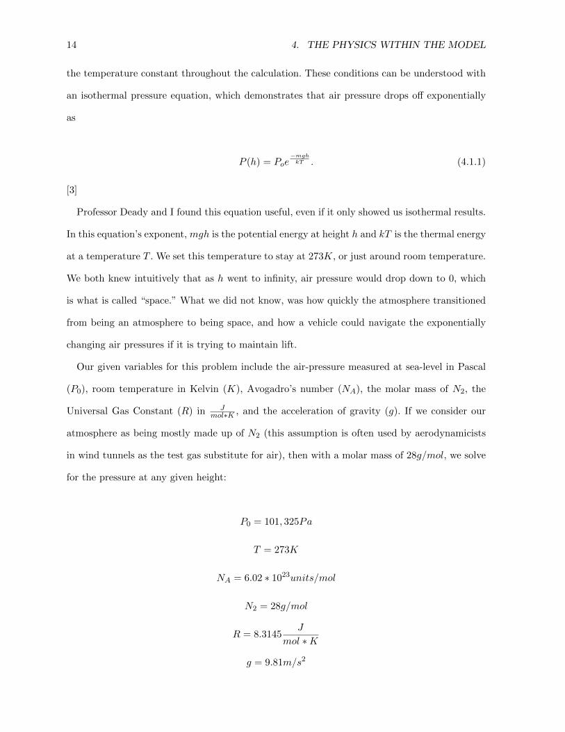
the temperature constant throughout the calculation. These conditions can be understood with

an isothermal pressure equation, which demonstrates that air pressure drops off exponentially

as

P (h) = Poe−mghkT . (4.1.1)

[3]

Professor Deady and I found this equation useful, even if it only showed us isothermal results.

In this equation’s exponent, mgh is the potential energy at height h and kT is the thermal energy

at a temperature T . We set this temperature to stay at 273K, or just around room temperature.

We both knew intuitively that as h went to infinity, air pressure would drop down to 0, which

is what is called “space.” What we did not know, was how quickly the atmosphere transitioned

from being an atmosphere to being space, and how a vehicle could navigate the exponentially

changing air pressures if it is trying to maintain lift.

Our given variables for this problem include the air-pressure measured at sea-level in Pascal

(P0), room temperature in Kelvin (K), Avogadro’s number (NA), the molar mass of N2, the

Universal Gas Constant (R) in Jmol∗K , and the acceleration of gravity (g). If we consider our

atmosphere as being mostly made up of N2 (this assumption is often used by aerodynamicists

in wind tunnels as the test gas substitute for air), then with a molar mass of 28g/mol, we solve

for the pressure at any given height:

P0 = 101, 325Pa

T = 273K

NA = 6.02 ∗ 1023units/mol

N2 = 28g/mol

R = 8.3145J

mol ∗K

g = 9.81m/s2

4.1. ATMOSPHERIC PHYSICS 15

k =R

NA= 1.38 ∗ 10−23J/K.

Using these variables to solve for the exponent mgkT , our equation for pressure becomes:

P (h) = P0 ∗ e−(0.121km−1)∗h. (4.1.2)

The pressures obtained from this equation are not completely accurate, given that the tem-

perature is held constant throughout, and the atmosphere is not entirely made up of N2. But

this model does show approximately how quickly air pressure drops off for a range of altitudes

that airplanes will see. In order to visualize this, I created a graph of the isothermal pressure

function that ranges from 0km altitude to 49.95km (with increments of 0.05km):

Figure 4.1.1. Air Pressure (Pa) as a function of Altitude (km) in isothermal conditions.

Air pressure drops off quickly as altitude increases. At sea-level the air pressure is 101, 325Pa,

but at an altitude of 10km, that pressure becomes 30, 214Pa. To give some context, 10km

(32, 808ft) is around the cruising altitude of most commercial airplanes (33, 000ft to 41, 000ft

for a Boeing 747). Thus, a commercial aircraft quickly experiences a range of air pressures during

ascent, which explains why your ears pop so frequently during a flight’s initial climb. The space


shuttle, which stays in a low-Earth orbit (ranges from 304km to 528km, or 190 to 330mi), indeed

begins its gliding descent in “space,” outside of our atmosphere. Design choices for an aircraft

that go to these high altitudes need to take into account the change in air density during the

trip.

4.1.2 Atmospheric Calculations: Adiabatic

I now move away from an isothermal calculation to an adiabatic, in order to visualize the change

in atmospheric temperature according to altitude.2 Temperature changes as you move to different

altitudes because of convection. When heat is applied to the bottom layer of a system, the hot,

less dense air rises while the cool, more dense air sinks. This can also be referred to as “vertical

mixing.” See figure 4.1.2 below.

Figure 4.1.2. In order to visualize convection, I drew a small diagram.

Convection has a number of effects on aviation and our atmosphere. The sun shines on our

planet and heats the ground. The air in the atmosphere is heated from below, and because of this,

atmospheric temperature changes at different heights, and atmospheric turbulence also occurs.

Atmospheric turbulence occurs when mixing air particles have small-scale, irregular motions that

are observed in winds with varying speed and direction. This effect is more extreme at lower

altitudes due to the increased flow disturbances around surface obstacles. To quantitatively

understand this, I calculated the adiabatic lapse rate3 for our atmosphere of N2.

2An adiabatic system is a system in which there is no heat transfer. That is, heat does not enter or leave the system.3Adiabatic Lapse Rate: The rate at which atmospheric temperature decreases with increasing altitude in conditions of

thermal equilibrium.

4.1. ATMOSPHERIC PHYSICS 17

Solving for a change in temperature over change in height involves splitting the height (which

we can call z) up into infinitely small slabs of length dz. Using the fact that we already know

the pressure as a function of height or z, we can also find dPdz . Then, in order to find the change

atmospheric temperature over a change in height, we can do

dT

dz=dT

dP∗ dPdz. (4.1.3)

For an ideal gas,4

PV = NkT. (4.1.4)

To complete this calculation, we also need the thermodynamic correction

PV γ = C, (4.1.5)

where C is a constant, and γ is the ratio of the specific heat coefficient at constant pressure

(Cp) and the specific heat coefficient at constant volume (Cv).

Then, solving for the volume V in equation 4.1.4, we obtain

V =NkT

P.

We can plug this volume into equation 4.1.5 to solve for C.

C = P ∗ NkTP

γ

.

We can now split up our equation for C: on one hand, we solve for the temperature T , and

on the other, we solve for ddP . In these two new equations, we define a new constant

C ′ ≡ (Nk)−γC.

4Note that although I’m using NkT instead of nRT , there is no difference because this term eventually cancels anyway.


Then, dividing out both equations, the constant C ′ cancels, and we can solve for dTdP . These

steps are shown below.

T :

T γ = P γ−1(Nk)−γC

T γ = P γ−1C ′ (4.1.6)

ddP :

(γ)T γ−1 dT

dP= (γ − 1)P γ−2C ′ (4.1.7)

Dividing equation 4.1.7 by equation 4.1.6:

(γ)T γ−1 dTdP = (γ − 1)P γ−2C ′

T γ = P γ−1C ′,

and we get

(γ)T−1 dT

dP= (γ − 1)P−1.

Finally,

dT

dP=γ − 1

γ(T

P). (4.1.8)

For a diatomic gas (assuming N2 is a good model for air),[3]

γ =CpCv

=(1

2)f + 1(2)

(12)f

=f + 2

f.

Using this γ, where f is the number of degrees of freedom in molecular motion, we can plug in

to equation 4.1.8 to find dTdP in terms of just f , T , and P . This simplified form lets us plug in

and solve for the dry adiabatic lapse rate, dTdz . Additionally, to find dP

dz , we take the derivative

of equation 4.1.1 in terms of height or z to find dPdz = −(mgkT )P . Putting it all together:

dT

dz= [(

2

5 + 2)(T

P)][−(

mg

kT)P ] = −(

2

7)(mg

k).

4.2. REYNOLDS NUMBER 19

For our rising air parcel, assuming it is made up of mostly nitrogen, we can solve for the dry

adiabatic lapse rate:

dT

dz= −(

2

7)[

(0.0288kg/mol)(9.81m/s2)

8.315J/K ∗mol] = −0.0097K/m = −9.7◦C/km (4.1.9)

This means that for every 1km increase in altitude, a body experiences a change in temperature

of about −10◦C. See figure 4.1.3.

Figure 4.1.3. A picture of convection in the atmosphere, resulting in a dry adiabatic lapse rate until about2km, where the atmosphere then becomes the free atmosphere and we reach the condensation level.[13]

4.2 Reynolds Number

Obtaining theoretical solutions of the flow field around a vehicle is difficult. Because of this,

experimental programs have been conducted to directly measure the parameters involved with

the flow field. In order to determine under what conditions the experimental results obtained

for one flow are applicable to another flow (which is confined by boundaries that are simply the

geometry of the aircraft), we can derive the Reynolds number, which is a dimensionless measure

of the ratio of inertial forces to viscous forces. Thus, the Reynolds number tells us that we can

manipulate the inertial properties of an aircraft (such as the chord width of an airfoil) to change

our movement through a fluid. It also tells us that the viscous properties of the fluid can change


the nature of the flow (higher viscous force, lower Reynolds number; higher inertial term, higher

Reynolds number). The objective of the parameters within the Reynolds number are as follows:[4]

1. To obtain information necessary to develop a flow model that could be used in numerical

solutions.

2. To investigate the effect of various geometric parameters on the flow field.

3. To measure directly the aerodynamic characteristics of a complete vehicle.

4. To verify numerical predictions of aerodynamic characteristics for a particular configuration.

Synthesizing these objectives, the Reynolds number gives us a numerical approach to the

particular geometric characteristics of a hybrid glide/powered vehicle. In addition, it helps us

understand the flow field around the entire vehicle. From this, we can identify what we can change

about the flight of an aircraft through air to optimize it for a particular air density and flow field.

Reynolds number (Re):

Re =Inertiaforce

V iscousforce=ρvl

µ=Ul

ν, (4.2.1)

[4]

where ρ is the density of the fluid, U is the velocity of the fluid (in the direction of the stream

of the fluid), l is the chord width of the particular airfoil, µ is the dynamic viscosity of the fluid,

and ν is the kinematic viscosity of the fluid. Increasing the inertial terms yields higher Reynolds

numbers, which means more laminar flow in the flow field. That is, the lower Re is, the more

sheet-like, smooth flowing the air is. At a higher Re, turbulence occurs as a results of differences

in speed and direction of the fluid. For every aircraft, big or small, different Reynolds numbers

drastically change the performance of that aircraft. Any aerospace program does not just study

the scale factor of the wings and rigid-body of an aircraft. The Reynolds number (Re) dictates

how that body will interact with the air flow around it.


Many external flows with which we are familiar with are associated with moderately sized

objects. These objects tend to have a characteristic length on the order of 0.01m < l < 10m. In

addition, typical upstream velocities are on the order of 0.01m??/s < U < 100m??/s, and the

fluids involved are typically water or air. The resulting Reynolds number range for such flows is

approximately 10 < Re < 109.

Flows with Re > 100 are dominated by inertial effects, whereas flows with Re < 1 are

dominated by viscous effects. Therefore, most familiar external flows are dominated by inertia.

Small Reynolds numbers mean that the viscous effects dominate, while large Reynolds numbers

mean that the inertial terms dominate. Thus, small Reynolds numbers characterize situations

where there is more turbulent flow around the object moving through the fluid. High Reynolds

numbers typically describe situations with more laminar flow.

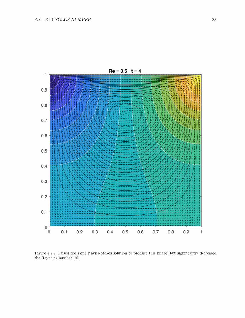
To visualize this, I’ve included a code that I have been working on in MATLAB, made available

by [10]. Pay attention to the direction of the arrows in the pictures, which shows the direction

of the velocity of a fluid particle at a particular point. In the case with a high Reynolds number,

there is more variation in the direction of the particle flow over the entire grid.


Figure 4.2.1. Consider a Navier-Stokes incompressible flow-field with a Reynolds number of 5.3560e7.Notice that the velocity vectors, which are visualized by the small arrows, are steady throughout the flowfield. That is, their direction does not vary as much as with a lower Reynolds number and turbulent flow.To read more about this solution to the Navier-Stokes equation, see [10].


Figure 4.2.2. I used the same Navier-Stokes solution to produce this image, but significantly decreasedthe Reynolds number.[10]


4.3 Lift and Drag

In order to solve for the forces on a plane in a flight path model, one must find out some

extremely difficult parameters about the aircraft. I was interested in being able to calculate the

lift and drag forces on an object so that I could solve for the energy loss due to drag in the

following chapter.

When a body moves through a fluid, its interaction between it and the fluid can be described

in terms of the stresses. The wall shear stresses on the body, τw, is due to viscous effects and

normal stresses due to the pressure p. Both τw and p vary in magnitude and direction along the

surface of an airfoil. See figure 4.5.1.

Figure 4.3.1. Provided by Munson, we can see the forces from the fluid surrounding a two dimensionalslice of a wing.[3]

Solving for lift and drag includes summing the pressure and stress forces on the top and

bottom surface areas of an object moving through a fluid. We obtain the lift and drag forces

on an object by integrating the effect of the pressure and shear forces on the body surface. The

pressure and shear forces on a small element of the surface of a body can be visualized like this:

The x and y components of the fluid force on the area element dA are, according to figure 4.5.1,

dFx = (pdA)cosθ + (τwdA)sinθ

4.3. LIFT AND DRAG 25

Figure 4.3.2. The pressure and shear force elements that affect the calculated lift and drag forces on anobject.[3]

and

dFy = −(pdA)sinθ + (τwdA)cosθ.

The lift and drag forces are thus,

L =

∫dFx =

∫(pcosθ)dA+

∫(τwsinθ)dA (4.3.1)

.

and

D =

∫dFx =

∫(pcosθ)dA+

∫(τwsinθ)dA. (4.3.2)

Both the shear force and pressure force contributes to the lift and drag. In order to calculate

lift and drag, you have to determine the the pressure and shear force distributions on the

body. From an engineering standpoint, this is where one wing differentiates itself from another.

Manipulating the shape of the wing changes the shear stress distribution and magnitude, as well

as the pressure distribution and magnitude. Additionally, the angle of attack clearly affects the


lift and drag of an airfoil and aircraft. Equations 4.5.1 and 4.5.2 are true for any body, but you

still have to find the appropriate shear stress and pressure distributions on a body. Instead of

this, I used a simplified method, which involves defining dimensionless lift and drag coefficients

(CL and CD respectively). These are defined as:

CL =L

12ρ ∗ U2A

(4.3.3)

CD =D

12ρ ∗ U2A

. (4.3.4)

A is the characteristic area of the object, which I take in my calculations to be the frontal area

(the projected area observed by someone looking toward the object from a direction normal to

the upstream velocity, or U).

Calculating the characteristic area involves breaking the airfoil up like so:

Figure 4.3.3. The frontal area of a finite, three-dimensional airfoil.[3]

I use this method of obtaining the area and solving for the drag coefficient CD to find the

drag force D and total energy of the model flight path.

Note a few properties of these formulas:

4.3. LIFT AND DRAG 27

1. Drag increases proportional to the upstream velocity squared. This would be parasite drag,

described in chapter 3. 2. The density of air ρ increases the drag force linearly. 3. The charac-

teristic area of the object increases the drag force linearly. 4. The coefficient of drag increases

linearly with the drag force (somewhat trivial).


5The Model Flight Plan

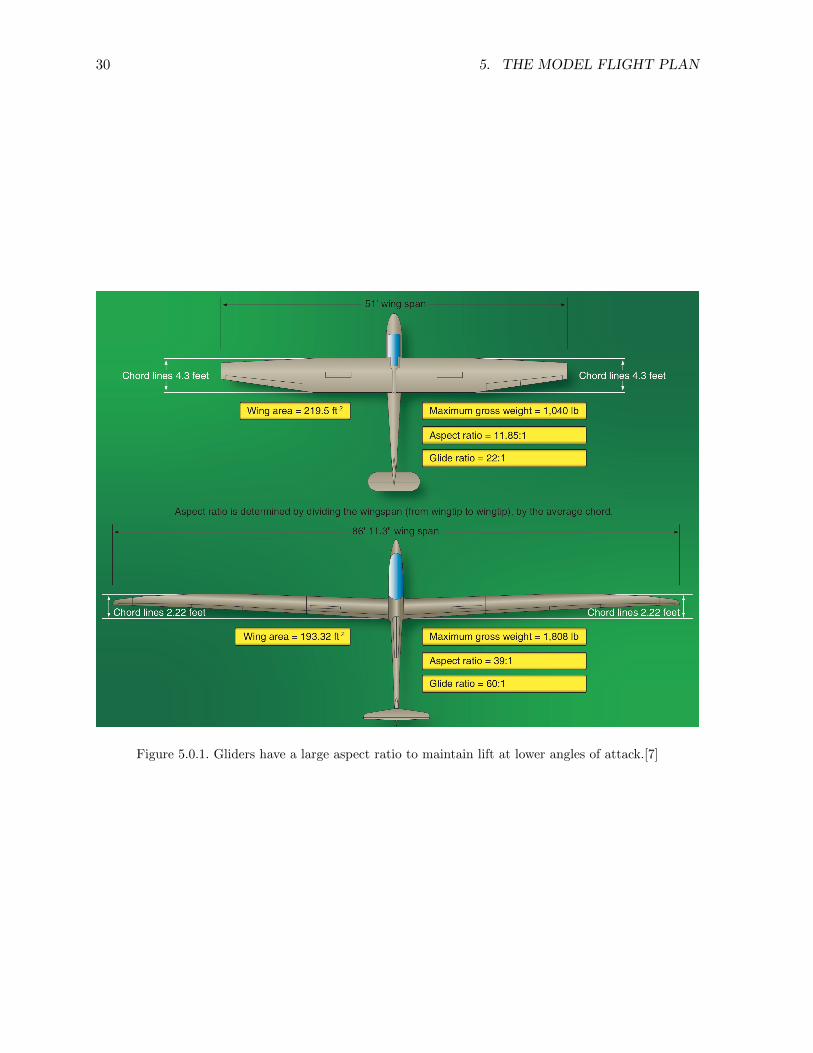
In designing the appropriate flight model, I used the following aspect ratio and design specifics

(figure 5.0.1), provided by the FAA glider handbook:

Matt and I made some assumptions about the flight of the aircraft to model a simple flight

path. We identified the total energy as the parameter of interest, . The velocity of the aircraft

is held constant so that the drag force is held constant. Additionally, we keep the density of the

fluid constant. See the following hand-drawn diagram to understand the modeled flight path in

the subsequent table of values.

I used the following parameters to model the energy-optimization flight path:

1. Characteristic area: 219.5ft2 = 20.39m21

2. Aircraft mass: 1040lb = 471.74kg

3. Reynolds Number: Re = 105

1The characteristic area and aircraft mass come from figure 5.1.1.

30 5. THE MODEL FLIGHT PLAN

Figure 5.0.1. Gliders have a large aspect ratio to maintain lift at lower angles of attack.[7]

31

4. Angle of decline: a = 3◦

5. Velocity: 73knots = 37.55m/s

6. Drag coefficient: CD = 0.12

For data Sets 1 and 2: the temperature is held constant at room temperature, 273K. For

data sets 3 and 4, temperature and air density at different altitudes reflects the U.S. Standard

Atmosphere measurements published by the United States in 1976.[5]. The aircraft velocity was

taken from an FAA document online that cited the best glide speed for a PA 28 161 (see [11]).The

drag force, using equation 4.3.4, depends on the characteristic area A, the upstream velocity U ,

the drag coefficient CD, and the air density, which depends on the temperature and air pressure

at a particular altitude.

The Drag coefficient and associated Reynolds number are set to values that ensure laminar

flow in the path of the vehicle.


5.1 Data Sets For Energy Optimization

When we modeled this flight, we visualized it in a simple geometric flight path. We held the

angle of descent, a, constant, so we could vary the angle of ascent b and observe how much

powered energy would be needed for different paths along the descent line, G. The maximum

height of the flight path h and the horizontal length component of the glide-path x were found

using trigonometric identities and a system of equations, shown at the top my drawing. The

total horizontal distance d of the flight path was held constant at 1000km.

The length of the gliding descent is labeled G, while the length of the powered ascent is L.

The relationship between these two lengths is of interest.

In data sets 1 and 2, the air pressure is calculated using the same air pressure formula derived

in chapter 4 (equation 4.1.2). This air pressure is used to calculate air density, using the equation

ρ = pRT [3]. The value used for the gas constant R is the SI value: R = 287.05N ∗m/kg ∗K.

In data sets 3 and 4, I did not calculate the air density, nor did I hold the temperature at a

constant room temperature. The values for air density (kg/m3) and temperature (K) are taken

from the Geometric U.S. Standard Atmosphere measurements published by the United States

in 1976[5].

The kinetic energy KE of the plane is calculated by taking 12mV

2 where m is the mass of

the vehicle and V is the aircraft velocity. The potential energy PE is found by calculating mgh

where m is the mass of the vehicle, g is the gravitational acceleration 9.81m/s2, and h is the

maximum height that the aircraft reaches before gliding.

Drag is calculated using D = (CD)12ρ ∗ U2A, which comes from the equation for the drag

coefficient found in chapter 4. Once I calculated the drag force D , I could then multiply it by

the length of the path of the plane to get a “Drag Energy.” This is used to solve for the Powered

Energy and Glide Energy. The drag energy is split up into two parts: a powered drag energy and

a glide drag energy. These values reflect the drag energy over the powered path and gliding path

of the aircraft, respectively. Thus, the drag glide energy (DGE) is proportional to the length G

5.1. DATA SETS FOR ENERGY OPTIMIZATION 33

and the drag powered energy (DPE) is proportional to the length L. In addition, notice that

the parameters affecting drag are CD, ρ, U2 (which is just the aircraft velocity V 2), and A.

What I call “Powered Energy” is calculated by adding the potential energy and the energy

lost due to drag. The potential energy reflects the amount of energy needed to reach a height

h. This value is considered to be equal to the amount of energy that the powered flight would

need to produce to get to that height. The energy lost to drag is considered to be equal and

opposite in sign to the energy needed for thrust to maintain the same velocity. Since velocity is

held constant, the drag force is equal and opposite to the thrust force. Thus, PoweredEnergy

is the amount of energy that the powered plane requires from its engine to ascend.

What I call “Glide Energy” is calculated by subtracting the drag energy, calculated over

the path of the glide flight G, from the kinetic energy KE. The glide energy is thus directly

proportional to the amount of drag. I solved for this energy because the drag energy for the glide

path comes directly out of the kinetic energy of the glider. I’m assuming that the glider can

maintain its velocity by manipulating its shape and creating parasite drag (for example, using

flaps to create more resistance to the flow). This energy reflects the amount of “free energy”

that the aircraft has cashed in from its potential energy. This energy is used to counteract drag

energy.

I’m more interested in energy exchanges than total energy. I care more about the transition

from one type of energy to another. Powered Energy tells me the sum of how much energy is

needed from an engine to get up to a height h and how much energy is needed to counteract

drag. Glide energy tells me how much kinetic energy I have (I bought this kinetic energy by

getting up to a height h) minus the amount of energy taken away by drag (on the glide flight

path G). The final calculation I made takes the difference of the Glide Energy and Powered

Energy to calculate “Energy Efficiency.” This value reflects the optimization parameter: when

the Energy Efficiency has the highest value, the plane has taken the optimal flight path to reduce

the amount of powered energy required and maximize the amount of glide energy achieved. I

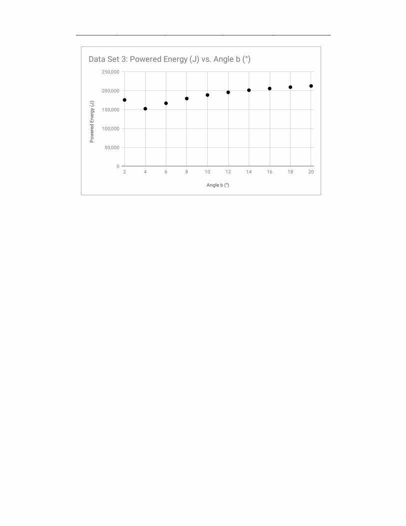
plotted the Powered Energy vs. Angle b and the Energy Efficiency vs. Angle b for all data sets.


5.1.1 Data Sets 1 and 2

Data Set 1:Angle a (°) Aircraft Mass (kg) Aircraft Velocity (m/s) Pressure (Pa) Temperature (K) Air Density (kg/m^3)

3 471.74 37.55 397 273 0.005063 471.74 37.55 431 273 0.005503 471.74 37.55 476 273 0.006073 471.74 37.55 537 273 0.006863 471.74 37.55 626 273 0.007993 471.74 37.55 764 273 0.009753 471.74 37.55 1000 273 0.012763 471.74 37.55 1473 273 0.018803 471.74 37.55 2702 273 0.034483 471.74 37.55 8026 273 0.10242

Data Set 2:Angle a (°) Glider Mass (kg) Aircraft Velocity (m/s) Pressure (Pa) Temperature (K) Air Density (kg/m^3)

3 471.74 37.55 764 273 0.009753 471.74 37.55 810 273 0.010343 471.74 37.55 864 273 0.011033 471.74 37.55 927 273 0.011833 471.74 37.55 1000 273 0.012763 471.74 37.55 1087 273 0.013873 471.74 37.55 1191 273 0.015193 471.74 37.55 1317 273 0.016813 471.74 37.55 1473 273 0.018803 471.74 37.55 1669 273 0.021303 471.74 37.55 1921 273 0.024523 471.74 37.55 2253 273 0.028753 471.74 37.55 2702 273 0.034483 471.74 37.55 3332 273 0.042523 471.74 37.55 4254 273 0.054293 471.74 37.55 5678 273 0.072453 471.74 37.55 8026 273 0.10242

h (km) d (km) x (km) d*tan(b) tan(a) tan(b) Angle b (°) L (km) G (km)45.81 1000 874.15 363.97 0.0524 0.3640 20 133.93 875.2245.12 1000 861.13 324.92 0.0524 0.3249 18 146.02 862.1844.30 1000 845.49 286.75 0.0524 0.2867 16 160.73 846.5343.30 1000 826.33 249.33 0.0524 0.2493 14 178.98 827.3442.04 1000 802.23 212.56 0.0524 0.2126 12 202.19 803.2140.40 1000 770.91 176.33 0.0524 0.1763 10 232.63 771.8538.17 1000 728.41 140.54 0.0524 0.1405 8 274.25 729.3134.97 1000 667.31 105.10 0.0524 0.1051 6 334.52 668.1329.95 1000 571.64 69.93 0.0524 0.0699 4 429.41 572.3420.96 1000 399.91 34.92 0.0524 0.0349 2 600.45 400.40

h (km) d (km) x (km) d*tan(b) tan(a) tan(b) Angle b (°) L (km) G (km)40.40 1000 770.91 176.33 0.0524 0.1763 10 232.63 771.8539.90 1000 761.54 167.34 0.0524 0.1673 9.5 241.78 762.4739.37 1000 751.40 158.38 0.0524 0.1584 9 251.69 752.3238.80 1000 740.40 149.45 0.0524 0.1495 8.5 262.48 741.3138.17 1000 728.41 140.54 0.0524 0.1405 8 274.25 729.3137.48 1000 715.30 131.65 0.0524 0.1317 7.5 287.16 716.1736.73 1000 700.89 122.78 0.0524 0.1228 7 301.36 701.7435.89 1000 684.97 113.94 0.0524 0.1139 6.5 317.06 685.8134.97 1000 667.31 105.10 0.0524 0.1051 6 334.52 668.1333.93 1000 647.59 96.29 0.0524 0.0963 5.5 354.04 648.3832.77 1000 625.42 87.49 0.0524 0.0875 5 376.01 626.1831.46 1000 600.31 78.70 0.0524 0.0787 4.5 400.93 601.0429.95 1000 571.64 69.93 0.0524 0.0699 4 429.41 572.3428.22 1000 538.58 61.16 0.0524 0.0612 3.5 462.28 539.2426.20 1000 500.04 52.41 0.0524 0.0524 3 500.65 500.6523.82 1000 454.51 43.66 0.0524 0.0437 2.5 546.01 455.0720.96 1000 399.91 34.92 0.0524 0.0349 2 600.45 400.40

KE (J) PE (J) Drag (N) Drag Powered Energy (J) Drag Glide Energy (J) DGE - DPE (J)332,577 211,977 8.74 1170 7646 6476332,577 208,819 9.49 1385 8181 6795332,577 205,028 10.48 1684 8869 7185332,577 200,382 11.83 2117 9788 7670332,577 194,537 13.78 2787 11071 8284332,577 186,941 16.81 3911 12976 9065332,577 176,637 22.01 6036 16052 10016332,577 161,820 32.42 10847 21664 10817332,577 138,620 59.47 25538 34039 8501332,577 96,977 176.68 106087 70742 -35344

KE (J) PE (J) Drag (N) Drag Powered Energy (J) Drag Glide Energy (J) DGE - DPE (J)332,577 186941 16.81 3911 12976 9065332,577 184670 17.84 4313 13603 9290332,577 182212 19.02 4788 14313 9524332,577 179544 20.40 5354 15122 9768332,577 176637 22.01 6036 16052 10016332,577 173456 23.92 6868 17130 10262332,577 169962 26.21 7898 18391 10493332,577 166103 28.99 9191 19881 10690332,577 161820 32.42 10847 21664 10817332,577 157037 36.74 13009 23824 10815332,577 151660 42.29 15902 26481 10580332,577 145572 49.59 19881 29804 9923332,577 138620 59.47 25538 34039 8501332,577 130603 73.34 33904 39549 5644332,577 121257 93.64 46883 46883 0332,577 110217 124.98 68239 56874 -11365332,577 96977 176.68 106087 70742 -35344

Powered Energy (J) (calories) (Btu)213,147 50870 202210,204 50168 199206,712 49335 196202,499 48329 192197,324 47094 187190,852 45549 181182,673 43597 173172,666 41209 164164,158 39178 155203,064 48464 192

Powered Energy (J) (calories) (Btu)190852 45549 181188983 45103 179187000 44630 177184898 44128 175182673 43597 173180325 43037 171177859 42449 168175294 41836 166172666 41209 164170046 40584 161167562 39991 159165453 39488 157164158 39178 155164508 39262 156168140 40129 159178457 42591 169203064 48464 192

Glide Energy (J) (calories) (Btu) Glide Efficiency (J)324,931 77549 308 111,784324,396 77422 307 114,192323,708 77257 307 116,996322,789 77038 306 120,290321,506 76732 304 124,182319,601 76277 303 128,749316,525 75543 300 133,852310,913 74204 294 138,247298,538 71250 283 134,381261,835 62490 248 58,771

Glide Energy (J) (calories) (Btu) Glide Efficiency (J)319,601 76277 303 128,749318,974 76127 302 129,991318,264 75958 301 131,264317,455 75765 301 132,557316,525 75543 300 133,852315,447 75286 299 135,122314,186 74985 298 136,327312,696 74629 296 137,401310,913 74204 294 138,247308,753 73688 292 138,707306,096 73054 290 138,534302,773 72261 287 137,320298,538 71250 283 134,381293,028 69935 278 128,521285,694 68185 271 117,554275,703 65800 261 97,246261,835 62490 248 58,771


5.1.2 Data Sets 3 and 4

Data sets 3 and 4 include values for air density (kg/m3) and temperature (K) taken from the

Geometric U.S. Standard Atmosphere measurements published by the United States in 1976[5].

Data Set 3:Angle a (°) Aircraft Mass (kg) Aircraft Velocity (m/s) Temperature (K) Air Density (kg/m^3)

3 471.74 37.55 266.373 0.0017623 471.74 37.55 264.164 0.0019133 471.74 37.55 261.403 0.0021933 471.74 37.55 258.641 0.0025273 471.74 37.55 255.878 0.0029953 471.74 37.55 251.456 0.0037703 471.74 37.55 244.818 0.0052093 471.74 37.55 236.513 0.0084633 471.74 37.55 226.509 0.0184103 471.74 37.55 217.581 0.075715

Data Set 4:Angle a (°) Glider Mass (kg) Aircraft Velocity (m/s) Temperature (K) Air Density (kg/m^3)

3 471.74 37.55 270.65 0.00383 471.74 37.55 227.5 0.00403 471.74 37.55 249.769 0.00443 471.74 37.55 262.147 0.00483 471.74 37.55 266.277 0.00523 471.74 37.55 270.409 0.00593 471.74 37.55 270.65 0.00663 471.74 37.55 255.878 0.00733 471.74 37.55 236.036 0.00853 471.74 37.55 260.771 0.00993 471.74 37.55 266.277 0.01023 471.74 37.55 269.031 0.01493 471.74 37.55 270.65 0.01843 471.74 37.55 266.925 0.02433 471.74 37.55 192.79 0.03373 471.74 37.55 258.019 0.04843 471.74 37.55 264.9 0.0757

h (km) d (km) x (km) d*tan(b) tan(a) tan(b) Angle b (°) L (km)45.81 1000 874.15 363.97 0.0524 0.3640 20 13445.12 1000 861.13 324.92 0.0524 0.3249 18 14644.30 1000 845.49 286.75 0.0524 0.2867 16 16143.30 1000 826.33 249.33 0.0524 0.2493 14 17942.04 1000 802.23 212.56 0.0524 0.2126 12 20240.40 1000 770.91 176.33 0.0524 0.1763 10 23338.17 1000 728.41 140.54 0.0524 0.1405 8 27434.97 1000 667.31 105.10 0.0524 0.1051 6 33529.95 1000 571.64 69.93 0.0524 0.0699 4 42920.96 1000 399.91 34.92 0.0524 0.0349 2 600

h (km) d (km) x (km) d*tan(b) tan(a) tan(b) Angle b (°) L (km)40.40 1000 770.91 176.33 0.0524 0.1763 10 23339.90 1000 761.54 167.34 0.0524 0.1673 9.5 24239.37 1000 751.40 158.38 0.0524 0.1584 9 25238.80 1000 740.40 149.45 0.0524 0.1495 8.5 26238.17 1000 728.41 140.54 0.0524 0.1405 8 27437.48 1000 715.30 131.65 0.0524 0.1317 7.5 28736.73 1000 700.89 122.78 0.0524 0.1228 7 30135.89 1000 684.97 113.94 0.0524 0.1139 6.5 31734.97 1000 667.31 105.10 0.0524 0.1051 6 33533.93 1000 647.59 96.29 0.0524 0.0963 5.5 35432.77 1000 625.42 87.49 0.0524 0.0875 5 37631.46 1000 600.31 78.70 0.0524 0.0787 4.5 40129.95 1000 571.64 69.93 0.0524 0.0699 4 42928.22 1000 538.58 61.16 0.0524 0.0612 3.5 46226.20 1000 500.04 52.41 0.0524 0.0524 3 50123.82 1000 454.51 43.66 0.0524 0.0437 2.5 54620.96 1000 399.91 34.92 0.0524 0.0349 2 600

G (km)875862847827803772729668572400

G (km)772762752741729716702686668648626601572539501455400

KE (J) PE (J) Drag (N) Drag Powered Energy (J) Drag Glide Energy (J) DGE - DPE (J)332,577 211,977 3.04 407 2660 2253332,577 208,819 3.30 482 2845 2363332,577 205,028 3.78 608 3202 2594332,577 200,382 4.36 780 3606 2826332,577 194,537 5.17 1044 4149 3105332,577 186,941 6.50 1513 5019 3506332,577 176,637 8.99 2464 6553 4089332,577 161,820 14.60 4884 9754 4870332,577 138,620 31.76 13637 18176 4539332,577 96,977 130.61 78424 52296 -26128

KE (J) PE (J) Drag (N) Drag Powered Energy (J) Drag Glide Energy (J) DGE - DPE (J)332,577 186940.92 6.50 1513 5019 3506332,577 184669.54 6.89 1666 5255 3589332,577 182211.99 7.52 1894 5661 3767332,577 179544.01 8.22 2158 6094 3936332,577 176636.87 8.99 2464 6553 4089332,577 173456.42 10.13 2908 7253 4345332,577 169961.65 11.43 3444 8019 4575332,577 166102.91 12.52 3970 8586 4617332,577 161819.55 14.60 4884 9754 4870332,577 157036.61 17.06 6038 11059 5020332,577 151660.42 17.60 6617 11020 4403332,577 145572.32 25.62 10274 15402 5128332,577 138619.74 31.76 13637 18176 4539332,577 130603.16 41.93 19386 22613 3227332,577 121256.56 58.17 29125 29125 0332,577 110217.17 83.57 45631 38031 -7600332,577 96977.11 130.61 78424 52296 -26128

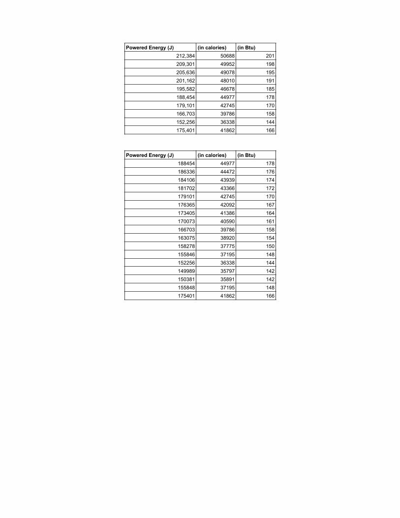
Powered Energy (J) (in calories) (in Btu)212,384 50688 201209,301 49952 198205,636 49078 195201,162 48010 191195,582 46678 185188,454 44977 178179,101 42745 170166,703 39786 158152,256 36338 144175,401 41862 166

Powered Energy (J) (in calories) (in Btu)188454 44977 178186336 44472 176184106 43939 174181702 43366 172179101 42745 170176365 42092 167173405 41386 164170073 40590 161166703 39786 158163075 38920 154158278 37775 150155846 37195 148152256 36338 144149989 35797 142150381 35891 142155848 37195 148175401 41862 166

Glide Energy (J) (in calories) (in Btu) Glide Efficiency (J)329,918 78739 312 117,534329,732 78695 312 120,432329,375 78610 312 123,739328,971 78513 312 127,809328,428 78384 311 132,846327,558 78176 310 139,104326,024 77810 309 146,923322,823 77046 306 156,120314,401 75036 298 162,145280,281 66893 265 104,880

Glide Energy (J) (in calories) (in Btu) Glide Efficiency (J)327,558 78176 310 139,104327,322 78120 310 140,986326,916 78023 310 142,810326,484 77920 309 144,782326,024 77810 309 146,923325,324 77643 308 148,960324,558 77460 307 151,153323,991 77325 307 153,919322,823 77046 306 156,120321,519 76735 305 158,444321,557 76744 305 163,280317,176 75698 300 161,330314,401 75036 298 162,145309,964 73977 294 159,976303,453 72423 287 153,071294,546 70297 279 138,698280,281 66893 265 104,880


5.2 Optimal Path

The Energy Efficiency plots show that there is a maximum value reached for lower values of b,

ranging from 4◦ to 6◦. The Powered Energy plots show that at that maximum Energy Efficiency

value, there is also a minimum amount of powered energy required from the aircraft. Notice

that for tiny angles of b, the powered energy gets very big in all cases. At this angle, the drag

powered energy overcomes the drag glide energy, which gives a negative value for DGE−DPE.

The parameters affecting drag are CD, ρ, U2 (which is just the aircraft velocity V 2), and A.

The only parameter that varies in this equation is ρ, which varies due to air density.2 Powered

Energy scales with height and drag. Glide Energy scales with drag. The optimal flight path

combines the geometry of the flight path which affects the powered energy, and the amount of

drag (related to the air densities at different altitudes) which affects the Glide Energy. Because

the weight and velocity of the aircraft is assumed constant, the kinetic energy term in the Glide

Energy is unchanging.

The Powered Energy relies on reducing h, and also reducing L. Because we assume that the

thrust force that the powered plane provides is equal to the drag force that we solve for, we

want our powered flight path to have as short a distance as possible.

Thus, the optimal flight path relies on reducing h and L as much as possible, while also

reducing the amount of drag over the entire trip. The drag depends on the altitude that the

aircraft reaches. The first set of data shows that the Energy Efficiency still has an optimal value

when the temperature is held constant. This confirmed for me that my pressure and air density

calculations were relatively accurate, even if they did not account for different layers of the

atmosphere where you see big differences in air pressure and density. The second sets of data,

3 and 4, provide an optimal Energy Efficiency for more accurate air pressure/density numerical

values.

2Note that the drag forces calculated tend to be low. This is due to a low coefficient of drag (also to the fact that theplane has small dimensions), which was held constant. When that coefficient is made bigger, the drag forces calculated scale

linearly.

6Conclusions

Given the assumptions and parameters detailed in chapter 5, there seems to be a way to reduce

the amount of powered energy required of an aircraft, and maximize the amount of glide energy

achieved by an aircraft. The Energy Efficiency plots reach a maximum value for lower angles of b,

between about 4◦ to 6◦. In summary, I am optimistic that there is a way to use glide technology

in the flight plan of a powered vehicle to reduce the amount of chemical energy needed from that

vehicle. I believe that this is done by optimizing the angle of powered ascent so that the aircraft

reaches lower values of h and L, and by generally reducing the types of drag contributing to the

model.

My goal with this plan was to reduce the amount of energy required from an engine by

designing a flight path that uses gliding to convert potential energy into kinetic energy. In

the future, there are more parameters that can be studied to make this model better from a

theoretical standpoint. For instance, we held the velocity constant throughout the trip, meaning

there must be something on the aircraft that increases drag during the glide descent to maintain

that velocity. In future work, it would be interesting to see how much speed can be gained from

an increasing kinetic energy on the glide path. This would mean letting gravity do its work on

the glide path. If one could pick up speed on the glide path, and then immediately go back

into the powered mode ascent/glide descent (and again pick up speed on the glide path), there

58 6. CONCLUSIONS

might be an interesting way to reduce the amount of energy needed from burning fuel while also

picking up speed from the gliding portion of the flight. It would thus be of interest to design a

flight plan that involves utilizing this hybrid glide/powered flight path more than once during

flight, perhaps to save on time, and efficiently increase aircraft velocity.

Bibliography

[1] McLean, D. (2018). Aerodynamic Lift, Part 1: The Science. The Physics Teacher, 56 (8), 516?520.

https://doi.org/10.1119/1.5064558

[2] McLean, D. (2018). Aerodynamic Lift, Part 2: A Comprehensive Physical Explanation. The Physics Teacher, 56 (8),521?524. https://doi.org/10.1119/1.5064559

[3] Munson, B. R., Okiishi, T. H., Huebsch, W. W., & Rothmayer, A. P. (2013). Fundamentals of Fluid Mechanics.

Instrumentation, Measurements, and Experiments in Fluids (7th ed.). https://doi.org/10.1201/b15874-3

[4] Bertin, J. J., & Russell M. Cummings. (2009). Aerodynamics For Engineers. (Tacy Quinn, Dee Bernhard, Scott Disanno,

& Rose Kernan, Eds.) (5th ed.). Upper Saddle River, NJ: Pearson Education, Inc.

[5] NASA. (1976, October 1). U.S. Standard Atmosphere 1976. 1976. Retrieved fromhttps://ntrs.nasa.gov/search.jsp?R=19770009539

[6] Denker, J. S. (n.d.). See How It Flies. Retrieved April 28, 2019, from http://www.av8n.com/how/htm/energy.html#fig-

pull-yoke-cruise

[7] FAA. (n.d.). Glider Handbook, Chapter 3: Aerodynamics of Flight. Retrieved fromhttps://www.faa.gov/regulations policies/handbooks manuals/aircraft/glider handbook/gfh ch03.pdf

[8] NASA. (n.d.). Space Shuttle Flying as a Glider. Retrieved October 1, 2018, from https://www.grc.nasa.gov/www/k-12/airplane/glidshuttle.html

[9] Bray, N. (2015). Space Shuttle and International Space Station. Retrieved fromhttps://www.nasa.gov/centers/kennedy/about/information/shuttle faq.html#14

[10] Seibold, B. (2008). A compact and fast Matlab code solving the incompressible Navier-Stokes equations on rectangulardomains mit18086 navierstokes.m. Retrieved from www-math.mit.edu/s̃eibold

[11] Safety Team, F. (n.d.). Best Glide Speed and Distance. Retrieved from http://1.usa.gov/2lYzSoN

[12] Atlantic, V. (n.d.). Learn - Virgin Galactic. Retrieved March 11, 2019, from https://www.virgingalactic.com/learn/

[13] Britannica. (n.d.). atmosphere: rising air in an unstable atmosphere. Retrieved April 1, 2019, from

https://kids.britannica.com/students/assembly/view/112173

[14] ATAG. (n.d.). Facts & figures. Retrieved April 1, 2019, from https://www.atag.org/facts-figures.html

Documents

Optimizing Glide-Flight Paths