1  

Optimum Dig Lines for Open Pit Grade Control

Isaaks, E, Ph.D., MausIMM, Geostatistical Consultant, Isaaks & Co., Email ed@isaaks.com

Treloar, I, Manager – Mine Technical Services, Newmont Mining Corporation, Email Ian.Treloar@newmont.com

Elenbaas, T, P.E., Consulting Geostatistician, Newmont Mining Corporation, Email Trevor.Elenbaas@newmont.com

ABSTRACT

Critical reviews of grade control generally focus on blast hole sampling and the estimation of ore control block model (OCM) grades with little or no attention given to dig line design. The estimation of block grades is deemed important as estimation errors lead to the misclassification of ore types and subsequent dollar loss. However, underestimation of block grades may be more or less costly than overestimation. Recognition of this problem led others to the application of loss functions for the assignment of ore type to individual OCM blocks. The method is known as MPS or maximum profit selection. However, each OCM block may be misclassified a second time by dig line design. Although each block may initially be assigned an optimum ore type, OCM blocks are seldom minable by ore type as individual blocks. A very common solution is the design of minable dig lines loosely constrained by a minimum mining width. These dig lines are often designed manually or by variations of computer generated contour lines and typically incur excessive dollar loss. This paper provides a method for constrained optimum dig line design where dig line misclassifications are also evaluated through loss functions or MPS. Constrained optimum dig line designs minimize the dollars lost by dig line misclassifications and are constrained by a minimum mining width. A case study is provided illustrating constrained optimum dig line design and subsequent benefits.

INTRODUCTION

Open pit grade control generally entails the sampling and assaying of blast hole cuttings followed by the estimation of ore control block model (OCM) grades. The estimated OCM block grades are then used in turn to design surface polygons or dig lines that outline and separate various ore types and waste material for the purposes of mining. Unfortunately, the estimation of block grades and the design of dig lines often results in the misclassification of ore types. For example:

True block grades are not known and must therefore, be estimated. If the classification of ore type based on the true but unknown block grade is different from the ore type based on the estimated block grade, then the ore type of the block is misclassified.

The locations of the true ore type contacts are not known and therefore their locations must also be estimated. Dig lines must be designed so that the contained ore type can actually be mined as designed by project mining equipment. If the dig line classification of ore type is different from the ore type classification based on block grade, then the block is misclassified. For example, a dig line containing a majority of blocks classified by grade as mill ore may include a small proportion of blocks classified by grade as waste. The waste blocks are misclassified by the dig line and as a result, will be sent to the mill.

 

Misclassaccumulablock grathe classiSrivastavapparent

Cdu

Ifcuwco

Ifwn

In other wtype maymisclassiestimatesvariance symmetrgreater th

One soluestimatiowhere the

where Z

constants

                  1 GeostatisB.L.U.E es

ification erroate. Interestiades has receification of ova, 1987; Deparadox:

Consider a truump are the f the truck isutoff grade,

waste, it doesosts. f the truck is

waste/mill cuothing is rec

words, the loy be greater tification of os1 such as krestimates arical. But, ashan those du

ution to the pon errors. Eqe loss due to

are Z are th

s. The estim

                       stical estimatorstimators or be

ors reduce reingly, the mieived considore types baseutsch, Magr

uck that has only two po

s sent to the ma relatively

s contain som

s sent to the dutoff grade, thcovered.

oss resultingthan the lossore type. Sririged estimatre calculateds the examplue to overesti

problem of asquation 1 ando underestim

L

he true and e

mation error e

                   rs that minimizest linear unbia

evenue. Theyisclassificatioderable attentsed on the beri, and Norre

just been loaossible destinmill, and thesmall dollar

me metal tha

dump, but thhe full poten

g from an unds resulting frivastava (19tes may not b

d by assuminle above illuimation.

symmetric lod Figure 1 pr

mation is grea

1

2

*( , Z)

*

cZ

c

estimated gra

e is calculat

e the variance ased estimators

y do not canon of OCM tion. For exaest1 estimateena, 2000). T

aded with mnations. e true grade o

loss will ocat will be rec

he true gradential dollar v

derestimatioom an overe87) points oube the best f

ng the loss restrates, the l

osses consisrovide an exater than the

Z Z Z

Z Z Z

ades, (.)L is

ted as e Z

of the distributs.

ncel one anotblocks resulample, severes are sub-opThe followin

muck pile ma

of the trucklccur because covered whic

e of the truckvalue of the t

on of grade aestimation ofut that minim

for grade conesulting fromlosses due to

ts of assignixample of an

loss due to o

Z

Z

the loss fun

Z .

ution of estimat

ther. They silting from thral authors hptimal (Schong example i

aterial and th

load is below although thch will offse

kload is greatruck load of

and misclassf grade and tmum error vntrol because

m over and uo underestim

ing loss func asymmetricoverestimati

nction, 1c and

tion errors are o

imply he estimationhave shown tofield, 1997; illustrates th

he mill and w

w the waste/mhe truckload et processing

ater than the f ore is lost –

ification of othe ensuing

variance e minimum e

underestimatimation may b

ctions to c loss functioion.

(1)

d 2c are

often referred t

2 

n of that

his

waste

mill is

g

–

ore

error ion is e far

on

to as

3  

Figure 1: An example of an asymmetric linear loss function where 1 2

198 and 66c c .

The estimate minimizing the expected loss for linear loss functions is the quantile of Z that corresponds to the ratio

1 1 2c c c . For the example in Figure 1 the estimate that minimizes the

expected loss is the 0.75 quantile of the probability distribution of Z . The probability distribution of Z can be obtained by conditional simulation methods (Davis, 1987; Deutsch, Magri, and Norrena, 2000; Isaaks, 1990). In all likelihood, the 0.75 quantile of the distribution of Z is greater than the mean. This would tend to increase the number of blocks classified above cutoff grade which would in turn increase the profit given that underestimation is costlier than overestimation. If this seems counter intuitive, consider a block whose kriged estimate is slightly less than the waste/ore cutoff grade. The kriged estimate would classify the block as waste, however, the 0.75 quantile of the probability distribution of Z may be above the cutoff grade, which would render the block as ore and reduce the dollar loss.

The ore type classification of OCM block grades by using loss functions of the block grades rather than by the block grades themselves is sometimes called MPS or maximum profit selection. Misclassification errors made by assigning an ore type to a block based on either the block grade or loss functions of the block grade are referred to as grade misclassifications.

The efficacy of MPS is frequently demonstrated by calculations based on “free selection” (Schofield, 1997; Deutsch, Magri, and Norrena, 2000; Dagdelen and Coskun, 1999). Free selection presupposes that each OCM block is equivalent to a selective mining unit (SMU) and each SMU can be mined and sent to the correct destination according to its classified ore type. In other words, none of the SMU will be misclassified or sent to the wrong destination at the time of mining. This presumption is not true in practice. The spatial configurations of SMU blocks with the same ore type are often very complex, rendering the mining of an individual SMU impractical. Moreover, many OCM models consist of blocks much smaller than an individual SMU.

A practical method for the layout of minable ore types is the design of dig lines constrained by a minimum mining width (MMW). In fact, most open pit mining operations have a designated ore control engineer or geologist who is tasked with the design of dig lines for each blast.

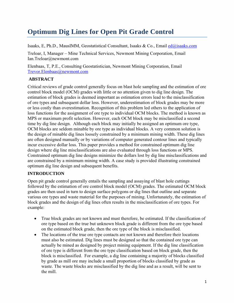
However, the design of dig lines is typically charged with additional misclassification errors. Figure 2 shows an example of an ore control block model overlain with dig lines. The various ore types are symbolized by different shades of grey. The two arrows illustrate the MMW. Admittedly, the blocks are smaller than the MMW or SMU, however, the misclassification of many OCM blocks by dig line design is obvious. These misclassification errors are referred to as dig line misclassification errors as opposed to grade misclassification errors.

 

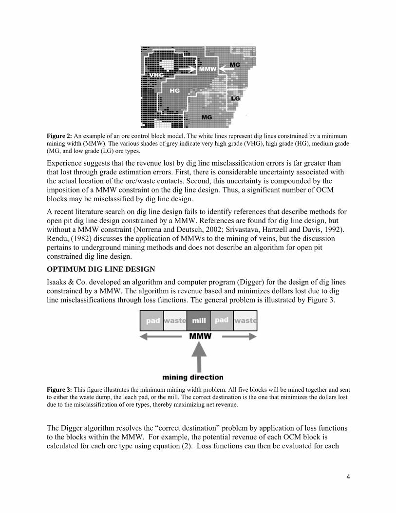
Figure 2: Amining wid(MG, and l

Experienthat lost tthe actuaimpositioblocks m

A recent open pit without aRendu, (pertains tconstrain

OPTIMU

Isaaks &constrainline misc

Figure 3: Tto either thdue to the m

The Diggto the blocalculate

An example ofdth (MMW). Tlow grade (LG

nce suggests through grad

al location ofon of a MMW

may be miscla

literature sedig line desia MMW con1982) discusto undergrou

ned dig line d

UM DIG LI

Co. developned by a MMclassification

This figure illuhe waste dump,misclassificatio

ger algorithmocks within td for each o

f an ore controlThe various shaG) ore types.

that the revede estimationf the ore/wasW constraintassified by d

earch on dig ign constrainnstraint (Norrsses the applund mining mdesign.

INE DESIG

ped an algorMW. The algns through lo

ustrates the min, the leach pad,on of ore types

m resolves ththe MMW. re type using

l block model. ades of grey ind

enue lost byn errors. Firsste contacts. t on the dig ldig line desig

line design fned by a MMrena and Delication of Mmethods and

GN

ithm and comorithm is rev

oss functions

nimum mining, or the mill. Ths, thereby maxi

he “correct dFor exampleg equation (2

The white linedicate very hig

dig line misst, there is coSecond, this

line design. gn.

fails to identMW. Refereneutsch, 2002;MMWs to thed does not de

mputer progvenue based s. The genera

width problemhe correct destimizing net rev

destination” pe, the potent2). Loss fun

es represent diggh grade (VHG

sclassificatioonsiderable us uncertaintyThus, a sign

tify referencnces are foun; Srivastava,e mining of vescribe an al

gram (Diggerd and minimial problem i

m. All five bloctination is the ovenue.

problem by tial revenue onctions can t

g lines constraG), high grade (

on errors is fauncertainty y is compounnificant numb

es that descrnd for dig lin, Hartzell anveins, but thgorithm for

r) for the desizes dollars lis illustrated

cks will be minone that minim

application oof each OCMthen be evalu

ained by a mini(HG), medium

far greater thassociated wnded by the ber of OCM

ribe methodsne design, bu

nd Davis, 199he discussionopen pit

sign of dig llost due to dby Figure 3

ned together anmizes the dollar

of loss functM block is uated for eac

4 

imum grade

han with

M

s for ut 92). n

ines ig . 

nd sent rs lost

tions

ch

5  

block and for each possible destination. The correct destination is the one where the combined dollar loss of all 5 blocks is minimum. $* * B , 1,n ore typesi i iP Z R i (2)

where

P = net revenue in dollars $ = metal price Z = block grade R = metallurgical recovery rate B = break even cost in dollars Zc = cutoff grade

Cutoff grades are almost always pre-defined by mining personnel, so the calculation of corresponding break even costs can be calculated using Equations (3). Note that each ore type is featured by a unique recovery function, , i 1,n ore types.iR

1 1 1

1 1 1 1

$* *

$*( * * ) 1, i i i i i i

B Zc R

B Zc R Zc R B i n ore types

(3)

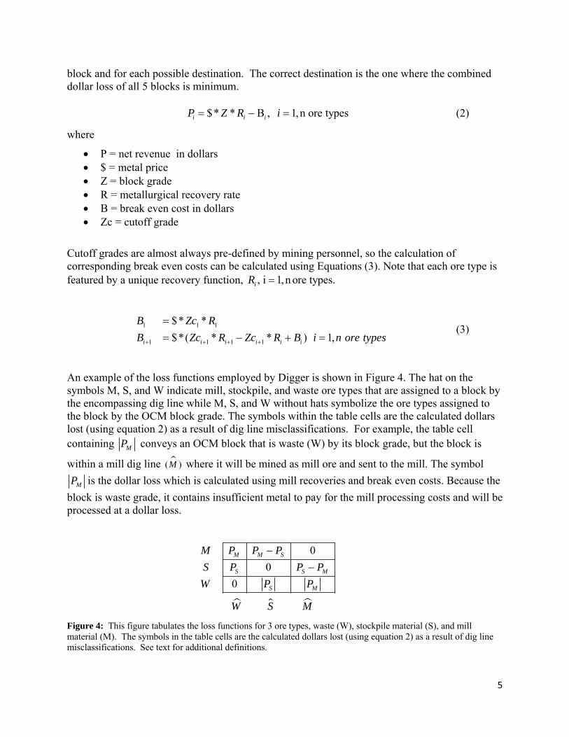
An example of the loss functions employed by Digger is shown in Figure 4. The hat on the symbols M, S, and W indicate mill, stockpile, and waste ore types that are assigned to a block by the encompassing dig line while M, S, and W without hats symbolize the ore types assigned to the block by the OCM block grade. The symbols within the table cells are the calculated dollars lost (using equation 2) as a result of dig line misclassifications. For example, the table cell containing MP conveys an OCM block that is waste (W) by its block grade, but the block is

within a mill dig line ( )M where it will be mined as mill ore and sent to the mill. The symbol

MP is the dollar loss which is calculated using mill recoveries and break even costs. Because the

block is waste grade, it contains insufficient metal to pay for the mill processing costs and will be processed at a dollar loss.

0

0

0

M M S

S S M

S M

M P P P

S P P P

W P P

W S M

Figure 4: This figure tabulates the loss functions for 3 ore types, waste (W), stockpile material (S), and mill material (M). The symbols in the table cells are the calculated dollars lost (using equation 2) as a result of dig line misclassifications. See text for additional definitions.

6  

The application of loss functions to groups of OCM blocks defined by a MMW is the key to Digger. Digger initially defines a mosaic of SMU type dig lines. Based on simulated annealing, Digger repeatedly iterates through the OCM testing the existing dig line locations. If a new dig line location can be found that reduces loss and does not violate the MMW, then the dig line is re-located to the new location. Digger continues iterating through the OCM until either no new dig line locations can be found or until a pre-defined number of iterations is reached.

CASE STUDY

The efficacy of constrained optimum dig line design is easily evaluated by comparing potential Digger revenues to those generated by other methods given an identical OCM. A simple summation of the ore type tonnes and grade generated by each set of dig lines is all that is needed. Differences between tonnes, grade, and revenue can only be due to differences between dig line designs.

In addition to providing an example comparing manually designed dig lines to optimum computer dig line designs, the case study also provides examples that focus on the impact of varying the MMW. Generally, once the MMW is defined it is seldom altered by grade control operations. Thus, the benefit of evaluating potential recoverable tonnes and grade by ore type as a function of MMW is typically not known. The MMW examples clearly illustrate the benefits of being able to rapidly evaluate potential dig line recoveries for various MMWs.

Although this study does not account for the uncertainty associated with the estimation of block grades, any accounting such as MPS would likely have very little impact on dig line misclassifications. Increases in net revenue as a consequence of assigning initial ore types to the OCM blocks by MPS would simply be in addition to revenue increases as a consequence of optimum dig line design.

The examples provided are based on actual mine data. However all grades, costs, and recoveries have been altered to preserve confidentiality. The case study considers data from a small open pit gold mine where oxide, transition and sulfide ore types exist. Ore type destinations are waste, leach pad, and mill.

Case study data

The OCM under study consists of 4,183 blocks, each measuring 2 m x 2 m x bench height. The OCM blocks are classified into 4 ore types plus some minor waste based on the oxide, transition, and sulfide classification rules described below.

Ore types

Sulfide mill (SuM) Transition mill (TrM) Oxide mill (OxM) Oxide leach (OxL) Waste (W)

Processing costs

Sulfide mill $ 30.00/tonne Transition mill $ 15.10/tonne

7  

Oxide mill $ 14.95/tonne Oxide leach $ 3.15/tonne

Metal prices

Au $1500.00/oz Ag $30.00/oz Cu $3.00/lb

Metal recovery

The metal recovery functions are complex non-linear functions of ore type and metal grades.

Oxide, transition, sulfide classification rules

If soluble copper > 1500 ppm or sulfide sulfur > 10% then ore type = sulfide else if soluble copper > 250 ppm then ore type = transition else if sulfide sulfur < 1.5% then ore type = oxide else if ratio of soluble gold to total gold < 0.6 ore type = transition else ore type = oxide

Computer program input (OCM block grades)

Total Au grade Soluble Au grade Ag grade Soluble copper grade Sulfide sulfur grade

Computer program output

Dig line tonnes and grade by ore type. Dig line revenue by ore type as a function of recoverable Au, Cu, and Ag. Dig line polygons

Manually designed dig lines versus Digger

This section compares dig line recoveries from a set of manually designed dig lines to those from a set of optimum dig lines designed by Digger. The manually designed dig lines by the company geologists were not available for this study, so we challenged an outside Ph.D. geologist with the task of constructing dig lines that minimize the misclassification of the OCM blocks while maintaining a MMW of 12 m or 6 blocks. The manual dig lines are shown in Figure 5 on the left. The Digger dig lines are shown by the map on the right side of Figure 5. Although the minimum mining width is 12 m or 6 blocks for both sets of dig lines, the white X’s drawn on the manual set of dig lines indicate MMW violations. The tiny squares in each map represent the original ore control block model. Ore types are identified by the grey scale. The labels in the maps indicate the dig line ore type.

 

Figure 5: Toptimal digis TrM; metype.

The relatTable 1. example,the in situpotentialrecoverabapproximcosts of Smisclassicontributfunctions

The 2.8%designs igenerally

Minimum

This sect18 m. Alwords, thmisclassi

This figure comg lines (on the edium grey is O

tive dig line All of the en, the total in u value of mly provide a ble ounces o

mately 116%SuM ore are ification of mtor to the mas or MPS.

O

% increase ins typical of w

y range betw

m mining w

tion comparel dig lines w

he dig lines aification by d

mpares a set ofright). The gre

OxM; light gre

tonnages, Antries in Tabsitu dollar v

material withi2.8% increa

of Au and Ag% more SuM

approximatmaterial withanual dig line

TaTable

re Type

(% OxL OxM TrM SuM Total

n net revenuewhat has gen

ween 2% to 5

width examp

es dig line rewere generateare physicalldig lines con

f manually desiey scale indicatey is OxL; and

Au and Ag oule 1 are perc

value of the min the manuaase in net revg compare vore tonnage

tely double thhin the SuM e dollar loss

able 1: Compae entries are %

Tonnes of manual)

85.4 111.3 110.5 87.2 99.2

e provided bnerally been%.

ples

ecoveries fored by Diggerly located bynstrained by

igned dig linestes the initial owhite is waste

unces, and docentages of tmaterial withal dig lines. venue over tery closely, than the opt

he cost of mdig lines is . This examp

arative Dig Linof manual dig

Au (wt % of manual)

83.3 114.9 103.0 84.5 100.5

y the optimun observed at

r 4 different r and the emy minimizinga minimum

s (on the left) toore type by bloce. The labels on

ollar revenuethe manual dhin the optimIn other wor

the manual sthe manual timum dig li

milling eithervery costly aple clearly il

ne Statistics. line quantities

Ag (wt %

of manual) 78.8

108.6 109.1 84.5

100.8

um computet other mines

MMWs, nammployment ofg the dollar lmining wid

o a set of compck grade; blackn the maps indi

es by ore typdig line quanmum dig linerds, the optimset of dig linedig lines conines. Note thr TrM or OxMand is likelyllustrates the

s. Revenue

(% of manual )

88.9 100.0 108.5 98.1

102.8

er dig lines os. Increases

mely 10 m, f loss functioloss due to th

dth.

puter generatedk is SuM ; darkicate the dig lin

pe are given ntities. For es is 102.8%mum dig lines. Althoughntain hat the proceM. Thus, the

y the major e value of lo

over manual in net revenu

12 m, 15 m, ons. In otherhe

8 

d k grey ne ore

in

% of nes h the

essing e

ss

ue

and r

 

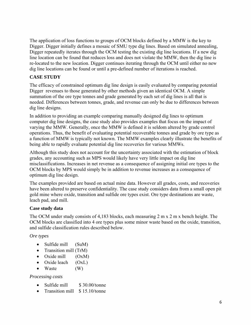
The 4 seteach mapare locateprocess.

Figure 6: Tand labels with less dresult of di

Summar

The dig lmisclassithe total r

ts of dig linep. For examped within a S

This figure shoindicate the or

dilution and oreigging error at

ry statistics

lines shown ification are revenue afte

es are shownple, near the SuM dig line

ows 4 sets of dre types as exple loss, the relatthe time of min

by MMW

in Figure 6 acomputed b

er dig line de

n in Figure 6center of th

e, e.g., these

ig lines constralained in Figurive simplicity oning.

are very effiby comparingesign. For ex

. Dig line mie MMW-12 are waste bl

ained by 10 m,re 5. Although of the 18 m MM

cient. For exg the total Oxample:

isclassificatimap, a num

locks that w

, 12 m, 15 m, athe 10 m MMWMW likely red

xample, the dOCM revenue

ions are cleamber of wastewill be sent to

and 18 m MMWW appears to bduces dilution a

dollars lost de before dig

arly visible ine blocks (who the SuM

Ws. The grey sbe more selectiand ore loss as

due to dig linline design t

9 

n hite)

scale ive, s a

ne to

10  

MW10 dig line loss = 1.36% of total OCM revenue; MW12 dig line loss = 1.99% of total OCM revenue; MW15 dig line loss = 2.56% of total OCM revenue; and MW18 dig line loss = 2.12% of total OCM revenue.

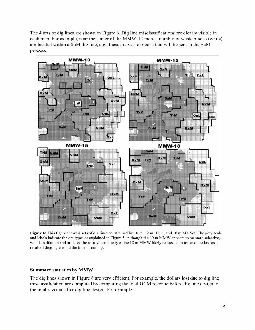
Table 2 is interesting because it shows that the total revenues attributable to each MMW compare very closely in spite of the increasing quantities of metal lost with larger MMWs. Although more ounces of Au and Ag are lost with larger MMWs, the recoverable metal grades are almost equivalent across all four MMWs. This is evident because revenue and tonnes are nearly equivalent across the four MMWs.

Table 2: MMW Statistics

Table entries are % of OCM quantities (no dig lines).

MMW ∑Rev

(% of OCM) ∑Tonnes

(% of OCM) Au Loss (wt%)

Ag Loss (wt%)

10 m 98.6 97.7 1.59 2.69 12 m 98.0 98.1 1.68 3.94 15 m 97.4 99.4 2.54 7.05 18 m 97.9 99.5 2.02 4.71

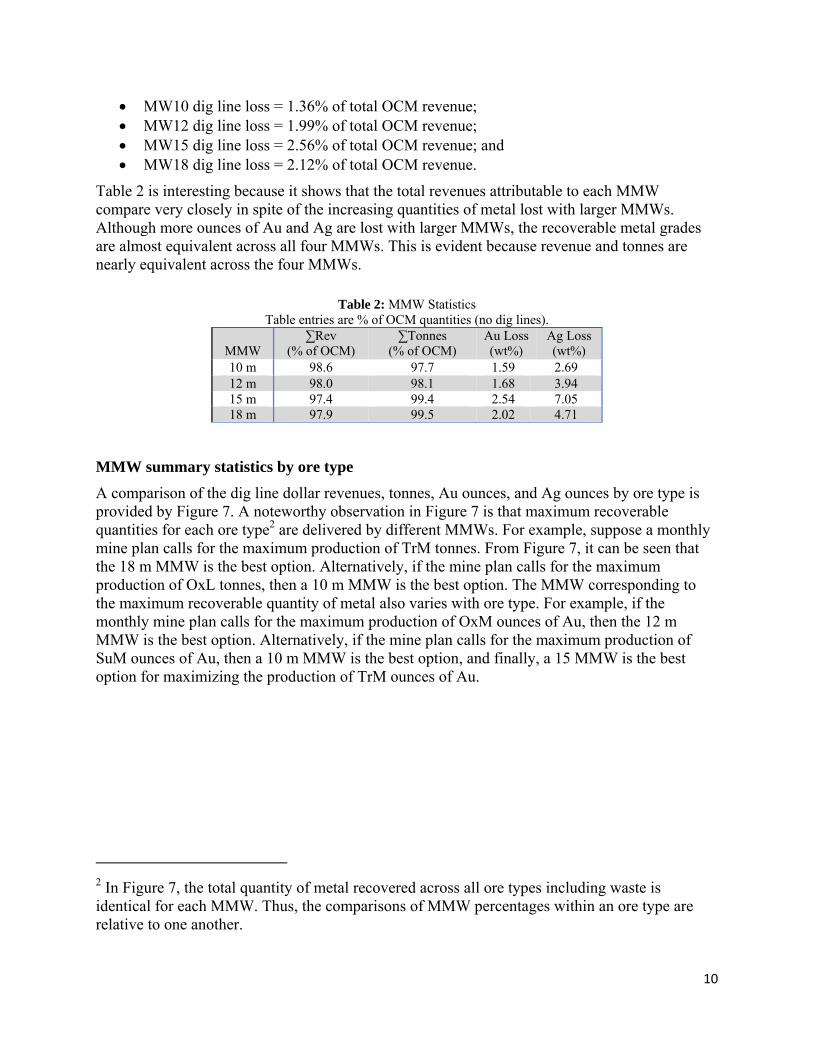
MMW summary statistics by ore type

A comparison of the dig line dollar revenues, tonnes, Au ounces, and Ag ounces by ore type is provided by Figure 7. A noteworthy observation in Figure 7 is that maximum recoverable quantities for each ore type2 are delivered by different MMWs. For example, suppose a monthly mine plan calls for the maximum production of TrM tonnes. From Figure 7, it can be seen that the 18 m MMW is the best option. Alternatively, if the mine plan calls for the maximum production of OxL tonnes, then a 10 m MMW is the best option. The MMW corresponding to the maximum recoverable quantity of metal also varies with ore type. For example, if the monthly mine plan calls for the maximum production of OxM ounces of Au, then the 12 m MMW is the best option. Alternatively, if the mine plan calls for the maximum production of SuM ounces of Au, then a 10 m MMW is the best option, and finally, a 15 MMW is the best option for maximizing the production of TrM ounces of Au.

                                                            

2 In Figure 7, the total quantity of metal recovered across all ore types including waste is identical for each MMW. Thus, the comparisons of MMW percentages within an ore type are relative to one another.

 

 

Figure 7: Aas the perc4.4% + 27.

Evidentlydig line dnumber oincrease.reasonabthis pointis a topic

CONCL

Computetool availline desigreturn inv

Oisgopeaeq

Cb

A comparison cent of total. Fo.4% + 22.7% +

y, the compldesign. Extreof dig line m On the othely well defint, an obvious

c for another

LUSIONS

er design of olable to the mgn are largelvestment wit

Optimum digs costly. At $old averaginptimal dig liasily be avoiquipment, pe

Computer digenefits of di

of recoverableor example, the+45.3% + 0.2%

lexity of the emely compl

misclassificater hand, in dned contactss question mpaper.

optimum digmining induly unrealizedth huge pote

g line design $1500US/ozng 0.5 g/t to tine designs cided by usinersonnel, or g line designfferent MMW

e quantities attre total potential% = 100%.

in situ ore tylex spatial cotions. Conseqdeposits whe, the problem

might be, “W

g lines conststry. As a cod. Constraineential gains:

maximizes n, the dollars the dump excan cost hunng optimized

samples aren enables oneWs or cutoff

ributable to eaclly recoverable

ype contact bonfigurationquently, the

ere the in situm of dig line

What about bl

rained by a Monsequence, ed optimum

net revenue.lost by send

xceeds $14,0dreds of thou

d computer de required. e to quickly f grades can

ch MMW by oe ounces Au as

boundaries ins of ore type

benefit of ou ore types ae misclassificlast moveme

MMW is a nthe benefits dig line des

. Material seding a single000.00. Oveusands of do

designed dig evaluate diffbe evaluated

ore type. All cossociated with t

influences the boundariesptimum dig

are relativelycation shoul

ent”? Good q

new and rela of constrainign is a low

ent to the wroe 600 tonne Oer the course ollars. Theselines. No ad

fferent dig lind in a few m

omparisons are the 10 m MMW

he efficiencys increase thline design

y continuousld be minimaquestion, but

atively unknoned optimumrisk – high

ong destinatOCM block of a year, su

e losses can dditional

ne designs. Tminutes enabl

11 

given

W is

y of he will

s with al. At t that

own m dig

tion of ub-

The ling

12  

the selection of a dig line set that best satisfies current short term mine plan targets or changes in the local patterns of mineral continuity as mining progresses through the deposit. This is not possible with manually designed dig lines. The numerous calculations required within a few seconds are too many for the human brain.

Computer dig line design enables rectangular MMWs. For example, the MMW in the direction of shovel travel may be wider or narrower than the MMW in the perpendicular direction. Rectangular dig lines may reduce loss where the patterns of mineralization form narrow bands or veins with a reasonably consistent strike and dip. Dig lines are easily designed in directions parallel to the strike of a vein system or a contact trace by an internal rotation of the OCM before dig line design.

Computer dig line design can be applied to resource/reserve risk assessment. For example, the uncertainty associated with the predictions of an annual production schedule is often studied by calculating the in situ recoverable tonnes and grade from multiple conditional simulations of drill hole data across the deposit. But these calculations are typically based on free selection which is unrealistic. Computer generated optimum dig lines permit realistic simulated recoveries of tonnes and grade for different MMWs which not only provide the means to explore various mining options, but also increase the accuracy of the study.

FUTURE WORK

Currently, Digger works with the OCM block grades as they are provided, no matter which block grade estimator is used. However, work is underway with the full implementation of MPS. Given this option, Digger will simulate a block probability distribution for each OCM block based on the LU decomposition of the covariance matrix (Davis, 1987). This will enable Digger to assign initial MPS ore types to each block which will subsequently be used for optimum dig line design. The combination of MPS applied to block grades and dig line design will further increase the value of recoverable ore at the time of mining.

REFERENCES

Dagdelen, K,. and Coskun, B., 1999, Optimizing grade control in open pit gold mining, SME Preprint Number 99-189.

Davis, M. W. 1987. Production of conditional simulations via the LU triangular decomposition of the covariance matrix. Mathematical Geology, Vol. 19, No.2.

Deutsch, C., Magri, E., and Norrena, K., 2000, Optimal grade control using geostatistics and economics: methodology and examples. SME Transactions, Vol. 308.

Isaaks, E. H., 1990, The application of Monte Carlo methods to the analysis of spatially correlated data: Ph.D. Dissertation, Stanford University, 213 p.

Norrena, K. P. and Deutsch, C. V., 2002, Optimal determination of dig limits for improved grade control, 30th International Symposium on Computer Applications in the Mineral Industries (APCOM)., Phoenix, Arizona.

Rendu, J., 1982, Computerized estimation of ore and waste zones in complex mineral deposits, SME-AIME Annual Meeting, Dallas, Texas.

13  

Schofield, N. and Rolley, P., 1997, Optimization of ore selection in mining: method and case studies. Mining Geology Conference Proceedings. AusIMM, Melbourne.

Srivastava, R.M., 1987, Minimum variance or maximum profitability?, CIM Bulletin, vol. 80, no. 901, pp 63-68.

Srivastava, M., Hartzell, D., and Davis, B., 1992, Enhanced metal recovery through improved grade control. 23rd Application of Computers and Operations Research in the Mineral Industry, Society for Mining, Metallurgy, and Exploration, Tucson, AZ, pp 243-249.