Embed Size (px)
Citation preview
IMPERIAL COLLEGE LONDON
Department of Earth Science and Engineering
Centre for Petroleum Studies
Optimum Selection of Artificial-Lift Systems for Russian Heavy-Oil Fields
With an Experimental Design
By
Jean-Nicolas La Marre
A report submitted in partial fulfilment of the requirements for
the MSc and/or the DIC
September 2011

II
DECLARATION OF OWN WORK
I declare that this thesis
Optimum Selection of Artificial-Lift Systems for Russian Heavy-Oil Fields With an Experimental Design
is entirely my own work and that where any material could be construed as the work of others, it is fully
cited and referenced, and/or with appropriate acknowledgement given.
Signature:
Name of student: Jean-Nicolas La Marre
Name of College supervisor: Matt Jackson
Name of Company supervisor: Sandra Fountain and Adriaan Andersen

III
ACKNOWLEDGEMENTS
I would like to thank Hess Inc. for providing the opportunity to carry on this project, and the permission
to publish results.
I am grateful for the guidance and feedback given by my supervisors Sandra Fountain (Hess Inc.),
Adriaan Andersen (Hess Inc.) and Matt Jackson (Imperial College).
Thanks to Hess Inc., for providing me with a sponsorship to pursue my studies at Imperial College.
Finally, I dedicate this work to my parents, for all their support, and to my father, for inspiring me to
pursue a career as a petroleum engineer.
IV
TABLE OF CONTENTS – MAIN BODY
Abstract ...........................................................................................................................................................................................1
Introduction ....................................................................................................................................................................................1
Well Modelling ...............................................................................................................................................................................2
Fluid Data ...................................................................................................................................................................................3
Inflow Data .................................................................................................................................................................................4
Equipment Data ..........................................................................................................................................................................4
Design of Experiments ...................................................................................................................................................................4
Pre-experimental Planning ..........................................................................................................................................................4
Response variable ...................................................................................................................................................................4
Choice of factors, range and levels .........................................................................................................................................5
Choice of Experimental Design ..................................................................................................................................................5
Experimental Planning ................................................................................................................................................................6
Naturally Flowing Scenario ....................................................................................................................................................6
Electrical Submersible Pump ..................................................................................................................................................6
Progressive Cavity Pump ........................................................................................................................................................6
Pump Model Selection ............................................................................................................................................................7
Statistical Analysis..........................................................................................................................................................................8
Naturally Flowing Scenario ........................................................................................................................................................8
Electrical Submersible Pump .................................................................................................................................................... 10
Progressive Cavity Pump .......................................................................................................................................................... 11
Results .......................................................................................................................................................................................... 12
Conclusions .................................................................................................................................................................................. 14
Recommendations for further study ............................................................................................................................................. 14
Nomenclature ................................................................................................................................................................................ 14
SI Metric Conversion Factor......................................................................................................................................................... 15
References .................................................................................................................................................................................... 15
Appendices ................................................................................................................................................................................... 16
TABLE OF CONTENTS – APPENDICES
Appendices ................................................................................................................................................................................... 16
A. Critical Literature Review .................................................................................................................................................. 16
B. Fluid Data – Methodology .................................................................................................................................................. 29
C. Fluid Data – Matching Results (μo) .................................................................................................................................... 32
D. Design Of Experiments – Choice of Experimental Design ................................................................................................. 33
E. Statistical Analysis – ESP & PCP ....................................................................................................................................... 34
V
LIST OF FIGURES – MAIN BODY
Figure 1: Volga-Ural Basin Location (after Belonin, 1998) ...........................................................................................................2
Figure 2: Downhole Equipment Drawing .......................................................................................................................................4
Figure 3: Cause-and-Effect Diagram (DOE) ..................................................................................................................................5
Figure 4: FC1200 – Pump Performance Chart (run at 55Hz) .........................................................................................................7
Figure 5: FC1600 – Pump Performance Chart (run at 55Hz) .........................................................................................................7
Figure 6: RA16 – Pump Performance Chart (run at 55Hz) ............................................................................................................7
Figure 7: FC2200 – Pump Performance Chart (run at 55Hz) .........................................................................................................7
Figure 8: NAT – Simulated vs. Predicted Liquid Rate Plot ............................................................................................................8
Figure 9: NAT – Model Report ......................................................................................................................................................8
Figure 10: NAT – Main Effects & Interactions ..............................................................................................................................9
Figure 11: NAT – Surface Plot .......................................................................................................................................................9
Figure 12: ESP – Main Effects & Interactions ............................................................................................................................. 10
Figure 13: ESP – Surface Plot ...................................................................................................................................................... 10
Figure 14: PCP – Main Effects & Interactions ............................................................................................................................. 11
Figure 15: PCP – Surface Plot ...................................................................................................................................................... 11
Figure 16: Statistical Summary (Main Effects & Interactions) .................................................................................................... 12
Figure 17: Surface Plots [L] – Reservoir Pressure (2500psig)...................................................................................................... 12
Figure 18: Surface Plots [H] – Reservoir Pressure (2500psig) ..................................................................................................... 12
Figure 19: Surface Plots [L] – Reservoir Pressure (2000psig)...................................................................................................... 13
Figure 20: Surface Plots [H] – Reservoir Pressure (2000psig) ..................................................................................................... 13
Figure 21: Surface Plots [L] – Reservoir Pressure (1500psig)...................................................................................................... 13
Figure 22: Surface Plots [H] – Reservoir Pressure (1500psig) ..................................................................................................... 13
Figure 23: Surface Plots [L] – Reservoir Pressure (1000psig)...................................................................................................... 13
Figure 24: Surface Plots [H] – Reservoir Pressure (1000psig) ..................................................................................................... 13
LIST OF FIGURES – APPENDICES
Figure B-1: KAS-5 [2007] – Black Oil Correlations (Bo) ............................................................................................................ 30
Figure B-2: KAS-5 [2007] – Black Oil Correlations (μo) ............................................................................................................. 31
Figure C-1: SVE-15 [2008] – Matching Results (μo) ................................................................................................................... 32
Figure C-2: NEM-11 [2009] – Matching Results (μo) .................................................................................................................. 32
Figure C-3: YUK-17 [2009] – Matching Results (μo) .................................................................................................................. 32
Figure D-1: Screening Design – Data Table (32 runs) ................................................................................................................. 33
Figure D-2: Screening Design – Frequency Analysis (32 runs) ................................................................................................... 33
Figure E-1: ESP – Simulated vs. Predicted Liquid Rate Plot ....................................................................................................... 34
Figure E-2: ESP – Model Report .................................................................................................................................................. 34
Figure E-3: PCP – Simulated vs. Predicted Liquid Rate Plot ....................................................................................................... 34
Figure E-4: PCP – Model Report .................................................................................................................................................. 34
VI
LIST OF TABLES – MAIN BODY
Table 1: B2 Samples (Experimental Design) – Main Fluid Properties ...........................................................................................3
Table 2: Guidelines for Designing Experiments (after Montgomery, 2005) ..................................................................................4
Table 3: Design Factors – Type / Levels / Range ...........................................................................................................................5
Table 4: NAT – Experimental Design (levels & range) .................................................................................................................6
Table 5: ESP – Experimental Design (levels & range) ...................................................................................................................6
Table 6: PCP – Experimental Design (levels & range)...................................................................................................................6
Table 7: PCM Pumps – Performance Specifications ......................................................................................................................8
LIST OF TABLES – APPENDICES
Table B-1: Available Fluid Samples ............................................................................................................................................. 29
Table B-2: Kasimovskoye B2 Samples – Main Fluid Properties ................................................................................................. 29
Table B-3: Samples KAS-5 & KAS-8 – PVT Model Inputs ........................................................................................................ 30
Table B-4: Range Parameters – Black Oil Correlations ............................................................................................................... 31
1
MSc Petroleum Engineering 2010-2011
Optimum Selection of Artificial-Lift Systems for Russian Heavy-Oil Fields With an Experimental Design Jean-Nicolas La Marre
Matt Jackson, Imperial College London
Sandra Fountain and Adriaan Andersen, Hess Inc.
Abstract The Volga-Ural basin is one of the most prolific petroleum provinces in Russia. During the 1990s, when evaluating the
licences to produce low viscous oil (0.5-100cP) from its Samara province, the electrical submersible pump was singled out as
the best lift option. Due to recent heavy-oil discoveries (0.5-900cP), the validity of the previous artificial-lift performance
study is uncertain. Therefore, the selection and the optimisation of the best artificial-lift system now play an important role for
the development of these fields to maximise the liquid production rate.
To assess the effect of different artificial-lift systems, a sensitivity analysis is usually carried out. The optimal approach is to
run a full sensitivity analysis, but the number of simulations needed to achieve it rapidly becomes excessive. For example, if
we consider 10 parameters with at least 3 levels of interest each, it will take around 20,000 simulations to perform the full
sensitivity study by varying one parameter at a time. Therefore, we are looking for any technique that could reduce the number
of simulations. Design of experiments is a formalised method of data collection and analysis. With such technique, the same
information as that acquired with the traditional one-factor-at-a-time experimentation can be implemented with significantly
fewer number of runs to derive equations for predicting the objective function (after Damsleth et al., 1992).
This study presents an experimental design applied to a real case study on heavy-oil fields from Russia. First, the prediction of
the inflow and outflow performance relationships was used to generate the liquid production rate for each simulation run.
Then, a number of three cases were considered: the naturally flowing scenario as the base case and two artificial-lift systems.
Each design was specifically optimised for each scenario based on statistical considerations to reduce as much as possible the
total number of runs required. The liquid production rates were then interpolated to map their distribution for each scenario.
The results from the analysis can be finally used as inputs to obtain a predicted value of liquid rate for a particular heavy-oil
field and finally make a choice on which artificial-lift system is best to be implemented.
The conclusions of the study indicate that using a fractional factorial design can provide the same information as a full
sensitivity analysis with 80% fewer simulations. The statistical and regression analyses show that the electrical submersible
pump continues to be a flexible lift option with a wide operating range to produce at high reservoir pressures with relatively
low viscosity. However, the progressive cavity pump proves to be a competitive alternative at low reservoir pressures.
Introduction
The Volga-Ural basin is one of the oldest and most prolific petroleum provinces in Russia, located between the Ural Mountains
in the east, the Volga River in the west and bordering the Caspian Sea in the South. The Samara region is established in the
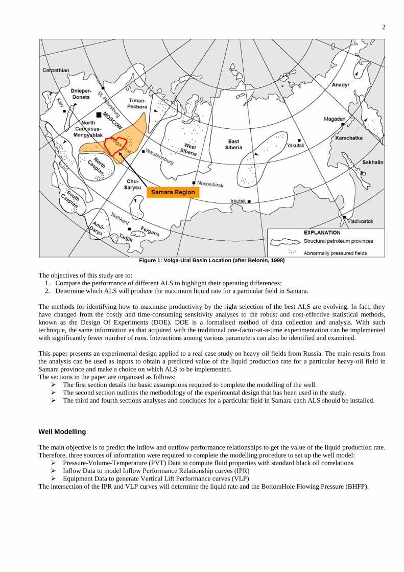
middle of the basin, where more than 150 oil reservoirs are currently at various stages of development (Figure 1). Reservoirs in
the South of that province are characterised by low temperature (30-50°C), high permeability (100-5000mD), low viscosity
(0.5-100cP) and low initial pressure (14-18MPa). During the evaluation of the licences to produce oil from these reservoirs, 10
years ago, the electrical submersible pump was singled out as the best option to lift and produce oil (Parfenov et al., 2008).
Historically, most production has been from this region where fluids with viscosity of 0.5 to 100cP are typical. Due to heavy-
oil discoveries in the Northern region of Samara, the practical experiences in artificial-lift performance gained in low viscous
oil fields from the South cannot be translated to develop heavy-oil fields in the North. Combining the difference in the maturity
of fields (low reservoir pressure and high water cut) with significant variations of viscosity (0.5-900cP), the selection and
optimisation of different Artificial-Lift Systems (ALS) now plays an important role for the development of heavy-oil fields in
that region to maximise the liquid production rate.
Imperial College London
2
Figure 1: Volga-Ural Basin Location (after Belonin, 1998)
The objectives of this study are to:
1. Compare the performance of different ALS to highlight their operating differences;
2. Determine which ALS will produce the maximum liquid rate for a particular field in Samara.
The methods for identifying how to maximise productivity by the right selection of the best ALS are evolving. In fact, they
have changed from the costly and time-consuming sensitivity analyses to the robust and cost-effective statistical methods,
known as the Design Of Experiments (DOE). DOE is a formalised method of data collection and analysis. With such
technique, the same information as that acquired with the traditional one-factor-at-a-time experimentation can be implemented
with significantly fewer number of runs. Interactions among various parameters can also be identified and examined.
This paper presents an experimental design applied to a real case study on heavy-oil fields from Russia. The main results from
the analysis can be used as inputs to obtain a predicted value of the liquid production rate for a particular heavy-oil field in
Samara province and make a choice on which ALS to be implemented.
The sections in the paper are organised as follows:
The first section details the basic assumptions required to complete the modelling of the well.
The second section outlines the methodology of the experimental design that has been used in the study.
The third and fourth sections analyses and concludes for a particular field in Samara each ALS should be installed.
Well Modelling
The main objective is to predict the inflow and outflow performance relationships to get the value of the liquid production rate.
Therefore, three sources of information were required to complete the modelling procedure to set up the well model:
Pressure-Volume-Temperature (PVT) Data to compute fluid properties with standard black oil correlations
Inflow Data to model Inflow Performance Relationship curves (IPR)
Equipment Data to generate Vertical Lift Performance curves (VLP)
The intersection of the IPR and VLP curves will determine the liquid rate and the BottomHole Flowing Pressure (BHFP).
3
Fluid Data
A total of 17 fluid samples are available, where at least for each reservoir one sample was tested and a fluid analysis reported.
However, given the relatively high number of samples, we clearly did not have time to run a full study and work on every
sample available. As Kasimovskoye is the only reservoir where more than two samples were tested, this field was used as a
reference reservoir to determine the black oil correlations that best fit the fluid data to be applied for the entire province.
The following methodology was performed to compare the samples to different standard black oil correlations:
The PVT reports associated to the samples available in this reservoir were reviewed and compared.
The measured data points were then compared to standard black oil correlations (Vasquez-Beggs, 1980; Glaso, 1980;
Standing, 1947; Lasater, 1958; Petrosky et al., 1993; Al-Marhoun, 1988) for the PVT properties such as Pb, Bo and
Gas-Oil Ratio (GOR). For μo, specific correlations (Beggs, 1995; Beal, 1946; Petrosky et al., 1995; Ng et al., 1983;
Bergman et al., 2007) were applied.
The comparison step involves graphical juxtapositions of the data with the correlations. It also includes checking the
coherence of the statistical regression results generated in PROSPERTM
when matching the measured data points.
Details of the results obtained for Kasimoskoye are described in the Appendix B, where it elaborates the previous methodology
applied to find the correlations. Finally, it concludes that Vasquez-Beggs and Beal correlations best fit respectively the main
PVT properties (Bo, GOR and ρo) and the viscosity (μo).
Even though Kasimovskoye is one of the three largest fields operated in the Northern licences, it was not practical to only work
on PVT data from this mature field. In particular, confining the study to viscosity from 450 to 550cP would have prevented
from playing with a wider viscosity range (100-900cP). Finally, it has been decided to target three PVT samples with
viscosities close to 100, 400 and 900cP from other reservoirs (respectively Svetogorskoye, Nemanoskoye and Yuknovskoye).
Therefore, based on the results from Kasimoskoye, Vasquez and Beal correlations were implemented to build the PVT models
of the three samples from reservoirs Svetogorskoye, Nemanoskoye and Yuknovskoye to be used for the experimental design.
Appendix C provides the matching results of the different samples considered for the experimental design; validating that
Vasquez-Beggs and Beal correlations still best reproduce the field data.
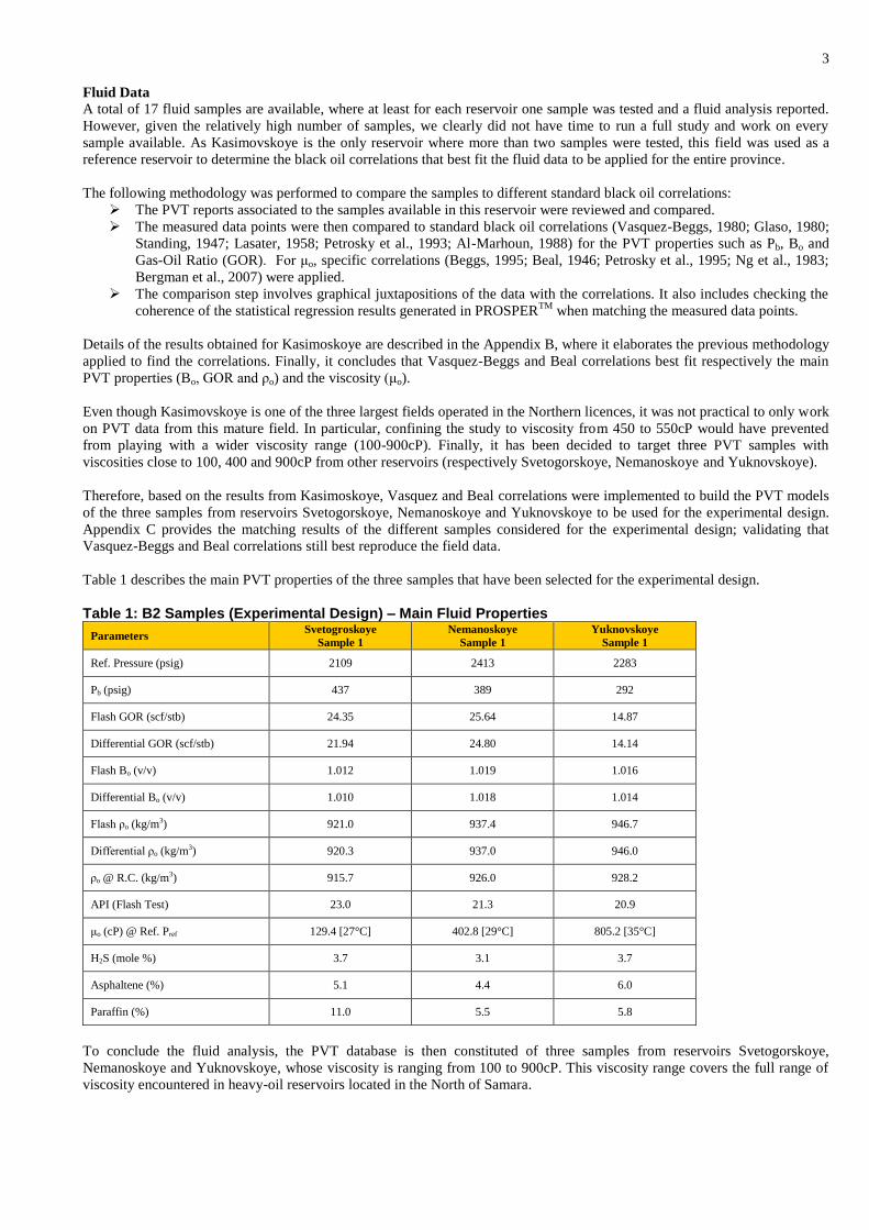
Table 1 describes the main PVT properties of the three samples that have been selected for the experimental design.
Table 1: B2 Samples (Experimental Design) – Main Fluid Properties
Parameters Svetogroskoye
Sample 1
Nemanoskoye
Sample 1
Yuknovskoye
Sample 1
Ref. Pressure (psig) 2109 2413 2283
Pb (psig) 437 389 292
Flash GOR (scf/stb) 24.35 25.64 14.87
Differential GOR (scf/stb) 21.94 24.80 14.14
Flash Bo (v/v) 1.012 1.019 1.016
Differential Bo (v/v) 1.010 1.018 1.014
Flash ρo (kg/m3) 921.0 937.4 946.7
Differential ρo (kg/m3) 920.3 937.0 946.0
ρo @ R.C. (kg/m3) 915.7 926.0 928.2
API (Flash Test) 23.0 21.3 20.9
μo (cP) @ Ref. Pref 129.4 [27°C] 402.8 [29°C] 805.2 [35°C]
H2S (mole %) 3.7 3.1 3.7
Asphaltene (%) 5.1 4.4 6.0
Paraffin (%) 11.0 5.5 5.8
To conclude the fluid analysis, the PVT database is then constituted of three samples from reservoirs Svetogorskoye,
Nemanoskoye and Yuknovskoye, whose viscosity is ranging from 100 to 900cP. This viscosity range covers the full range of
viscosity encountered in heavy-oil reservoirs located in the North of Samara.
4
Inflow Data
IPR curves are calculated from a straight-line inflow relationship incorporated into a well model. Due to Russian regulations
prohibiting the BHFP from falling below Pb, the inflow model is based on the simple equation shown below:
Q = PI (Pformation – Pflowing), where PI refers to the liquid Productivity Index in bbl/d.psi.
Equipment Data
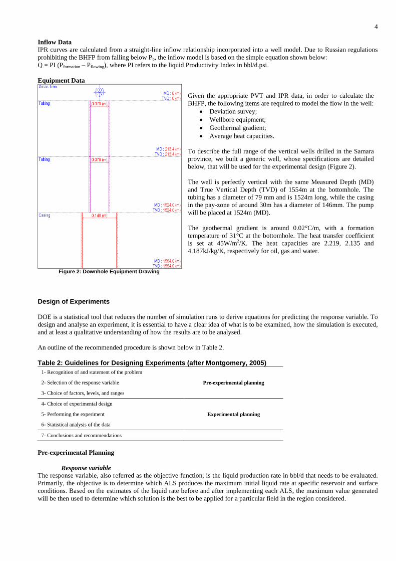
Figure 2: Downhole Equipment Drawing
Given the appropriate PVT and IPR data, in order to calculate the
BHFP, the following items are required to model the flow in the well:
Deviation survey;
Wellbore equipment;
Geothermal gradient;
Average heat capacities.
To describe the full range of the vertical wells drilled in the Samara
province, we built a generic well, whose specifications are detailed
below, that will be used for the experimental design (Figure 2).
The well is perfectly vertical with the same Measured Depth (MD)
and True Vertical Depth (TVD) of 1554m at the bottomhole. The
tubing has a diameter of 79 mm and is 1524m long, while the casing
in the pay-zone of around 30m has a diameter of 146mm. The pump
will be placed at 1524m (MD).
The geothermal gradient is around 0.02°C/m, with a formation
temperature of 31°C at the bottomhole. The heat transfer coefficient
is set at 45W/m2/K. The heat capacities are 2.219, 2.135 and
4.187kJ/kg/K, respectively for oil, gas and water.
Design of Experiments
DOE is a statistical tool that reduces the number of simulation runs to derive equations for predicting the response variable. To
design and analyse an experiment, it is essential to have a clear idea of what is to be examined, how the simulation is executed,
and at least a qualitative understanding of how the results are to be analysed.
An outline of the recommended procedure is shown below in Table 2.
Table 2: Guidelines for Designing Experiments (after Montgomery, 2005)
1- Recognition of and statement of the problem
Pre-experimental planning 2- Selection of the response variable
3- Choice of factors, levels, and ranges
4- Choice of experimental design
Experimental planning 5- Performing the experiment
6- Statistical analysis of the data
7- Conclusions and recommendations
Pre-experimental Planning
Response variable
The response variable, also referred as the objective function, is the liquid production rate in bbl/d that needs to be evaluated.
Primarily, the objective is to determine which ALS produces the maximum initial liquid rate at specific reservoir and surface
conditions. Based on the estimates of the liquid rate before and after implementing each ALS, the maximum value generated
will be then used to determine which solution is the best to be applied for a particular field in the region considered.
5
Choice of factors, range and levels
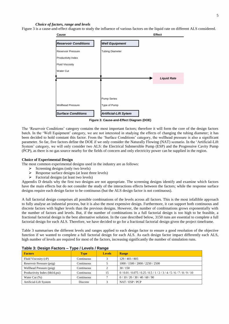
Figure 3 is a cause-and-effect diagram to study the influence of various factors on the liquid rate on different ALS considered.
Cause Effect
Reservoir Conditions Well Equipment
Reservoir Pressure Tubing Diameter
Productivity Index
Fluid Viscosity
Water Cut
Pump Series
Wellhead Pressure Type of Pump
Surface Conditions Artificial-Lift Sytem
Liquid Rate
Figure 3: Cause-and-Effect Diagram (DOE)
The ‘Reservoir Conditions’ category contains the most important factors; therefore it will form the core of the design factors
batch. In the ‘Well Equipment’ category, we are not interested in studying the effects of changing the tubing diameter; it has
been decided to hold constant this factor. From the ‘Surface Conditions’ category, the wellhead pressure is also a significant
parameter. So far, five factors define the DOE if we only consider the Naturally Flowing (NAT) scenario. In the ‘Artificial-Lift
System’ category, we will only consider two ALS: the Electrical Submersible Pump (ESP) and the Progressive Cavity Pump
(PCP), as there is no gas source nearby for the fields of concern and only electricity power can be supplied in the region.
Choice of Experimental Design
The most common experimental designs used in the industry are as follows:
Screening designs (only two levels)
Response surface designs (at least three levels)
Factorial designs (at least two levels)
Appendix D details why the first two designs are not appropriate. The screening designs identify and examine which factors
have the main effects but do not consider the study of the interactions effects between the factors; while the response surface
designs require each design factor to be continuous (but the ALS design factor is not continuous).
A full factorial design comprises all possible combinations of the levels across all factors. This is the most infallible approach
to fully analyse an industrial process, but it is also the most expensive design. Furthermore, it can support both continuous and
discrete factors with higher levels than the previous designs. However, the number of combinations grows exponentially with
the number of factors and levels. But, if the number of combinations in a full factorial design is too high to be feasible, a
fractional factorial design is the best alternative solution. In the case described below, 3150 runs are essential to complete a full
factorial design for each ALS. Therefore, we have decided to go for a fractional factorial design given the project timeframe.
Table 3 summarises the different levels and ranges applied to each design factor to ensure a good resolution of the objective
function if we wanted to complete a full factorial design for each ALS. As each design factor impact differently each ALS,
high number of levels are required for most of the factors, increasing significantly the number of simulation runs.
Table 3: Design Factors – Type / Levels / Range
Factors Type Levels Range
Fluid Viscosity (cP) Continuous 3 129 / 403 / 805
Reservoir Pressure (psig) Continuous 5 1000 / 1500 / 2000 / 2250 / 2500
Wellhead Pressure (psig) Continuous 2 30 / 150
Productivity Index (bbl/d.psi) Continuous 15 0 / 0.01 / 0.075 / 0.25 / 0.5 / 1 / 2 / 3 / 4 / 5 / 6 / 7 / 8 / 9 / 10
Water Cut (%) Continuous 7 0 / 10 / 20 / 30 / 40 / 60 / 90
Artificial-Lift System Discrete 3 NAT / ESP / PCP
6
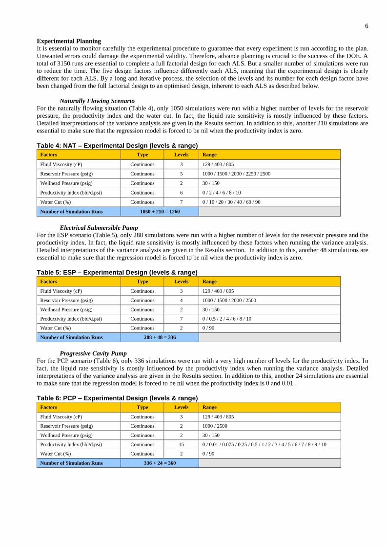
Experimental Planning
It is essential to monitor carefully the experimental procedure to guarantee that every experiment is run according to the plan.
Unwanted errors could damage the experimental validity. Therefore, advance planning is crucial to the success of the DOE. A
total of 3150 runs are essential to complete a full factorial design for each ALS. But a smaller number of simulations were run
to reduce the time. The five design factors influence differently each ALS, meaning that the experimental design is clearly
different for each ALS. By a long and iterative process, the selection of the levels and its number for each design factor have
been changed from the full factorial design to an optimised design, inherent to each ALS as described below.
Naturally Flowing Scenario
For the naturally flowing situation (Table 4), only 1050 simulations were run with a higher number of levels for the reservoir
pressure, the productivity index and the water cut. In fact, the liquid rate sensitivity is mostly influenced by these factors.
Detailed interpretations of the variance analysis are given in the Results section. In addition to this, another 210 simulations are
essential to make sure that the regression model is forced to be nil when the productivity index is zero.
Table 4: NAT – Experimental Design (levels & range)
Factors Type Levels Range
Fluid Viscosity (cP) Continuous 3 129 / 403 / 805
Reservoir Pressure (psig) Continuous 5 1000 / 1500 / 2000 / 2250 / 2500
Wellhead Pressure (psig) Continuous 2 30 / 150
Productivity Index (bbl/d.psi) Continuous 6 0 / 2 / 4 / 6 / 8 / 10
Water Cut (%) Continuous 7 0 / 10 / 20 / 30 / 40 / 60 / 90
Number of Simulation Runs 1050 + 210 = 1260
Electrical Submersible Pump
For the ESP scenario (Table 5), only 288 simulations were run with a higher number of levels for the reservoir pressure and the
productivity index. In fact, the liquid rate sensitivity is mostly influenced by these factors when running the variance analysis.
Detailed interpretations of the variance analysis are given in the Results section. In addition to this, another 48 simulations are
essential to make sure that the regression model is forced to be nil when the productivity index is zero.
Table 5: ESP – Experimental Design (levels & range)
Factors Type Levels Range
Fluid Viscosity (cP) Continuous 3 129 / 403 / 805
Reservoir Pressure (psig) Continuous 4 1000 / 1500 / 2000 / 2500
Wellhead Pressure (psig) Continuous 2 30 / 150
Productivity Index (bbl/d.psi) Continuous 7 0 / 0.5 / 2 / 4 / 6 / 8 / 10
Water Cut (%) Continuous 2 0 / 90
Number of Simulation Runs 288 + 48 = 336
Progressive Cavity Pump
For the PCP scenario (Table 6), only 336 simulations were run with a very high number of levels for the productivity index. In
fact, the liquid rate sensitivity is mostly influenced by the productivity index when running the variance analysis. Detailed
interpretations of the variance analysis are given in the Results section. In addition to this, another 24 simulations are essential
to make sure that the regression model is forced to be nil when the productivity index is 0 and 0.01.
Table 6: PCP – Experimental Design (levels & range)
Factors Type Levels Range
Fluid Viscosity (cP) Continuous 3 129 / 403 / 805
Reservoir Pressure (psig) Continuous 2 1000 / 2500
Wellhead Pressure (psig) Continuous 2 30 / 150
Productivity Index (bbl/d.psi) Continuous 15 0 / 0.01 / 0.075 / 0.25 / 0.5 / 1 / 2 / 3 / 4 / 5 / 6 / 7 / 8 / 9 / 10
Water Cut (%) Continuous 2 0 / 90
Number of Simulation Runs 336 + 24 = 360
7
Pump Model Selection
The experimental planning shows that we did not consider any pump characteristics in the procedure. In fact, the optimisation
process of the ALS itself shall be considered as a subset of the DOE. For each run, the pump model associated with its speed is
manually optimised on PROSPERTM
to make sure that the maximum liquid rate is captured.
The efficiency of the PCP can save up to 10 to 50% of the entire energy consumption compared to the ESP. We have assumed
that the PCP saves up 30% of the total energy demand from the ESP. After normalising the operating speed of the two ALS
(40-70Hz for ESP & 100-350rpm for PCP) to a scale from 0 to 100, it was easier to match where each ALS consumes the same
amount of energy. Therefore, for the same energy consumption, an ESP would operate at 55Hz and a PCP at 295rpm.
The final objective is to superimpose surfaces of the liquid rate for ESP & PCP. In fact, each set of surfaces is a collection of
discrete data points generated from a database of several pump models. Therefore, the regression model is the transformation
of discrete pumps to a continuous pseudo-pump that describes where the liquid rate is maximised at each simulation run.
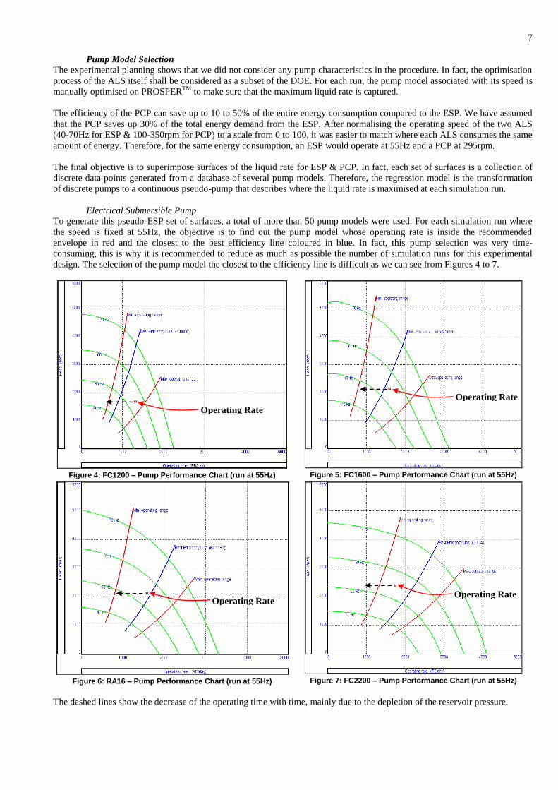
Electrical Submersible Pump
To generate this pseudo-ESP set of surfaces, a total of more than 50 pump models were used. For each simulation run where
the speed is fixed at 55Hz, the objective is to find out the pump model whose operating rate is inside the recommended
envelope in red and the closest to the best efficiency line coloured in blue. In fact, this pump selection was very time-
consuming, this is why it is recommended to reduce as much as possible the number of simulation runs for this experimental
design. The selection of the pump model the closest to the efficiency line is difficult as we can see from Figures 4 to 7.
Figure 4: FC1200 – Pump Performance Chart (run at 55Hz)
Figure 5: FC1600 – Pump Performance Chart (run at 55Hz)
Figure 6: RA16 – Pump Performance Chart (run at 55Hz)
Figure 7: FC2200 – Pump Performance Chart (run at 55Hz)
The dashed lines show the decrease of the operating time with time, mainly due to the depletion of the reservoir pressure.
Operating Rate
Operating Rate
Operating Rate Operating Rate
8
In that particular case, we would prefer to use pump FC1600 even though pump RA16 is producing at a higher rate. In fact, the
operating rate is more prone to decrease against time along the life of the ESP; it is then preferable to target the operating rate
to be on the right side of the efficiency line (pump FC1600) rather than on the left side (pump RA16). Therefore, the
decreasing rate will stay closer to the best efficiency line and longer compared to pump RA16.
Progressive Cavity Pump
To generate this pseudo-PCP set of surfaces, a total of four pump models were used, whose technical specifications are
described in Table 7. For each simulation run where the speed is aimed at 295rpm, all the four pumps are tested and the
maximum value of liquid rate achieved is selected. But, it is clearly not realistic to use any pump that will produce a rate below
half its validated capacity. For instance, when the generated rate at 295rpm for pump 86E2000 is below 927bbl/d, therefore
pump 60E2400 is the pump to use to comply with the threshold. The same procedure is applied to pumps 60E2400 & 24E2000.
Table 7: PCM Pumps – Performance Specifications
Manufacturer Pump Series Pump Model Outer Diameter
(inch)
Validated Capacity
(bbl/d)
PCM MOINEAU 2.7/8”EU 13E2000 2.875 280
PCM MOINEAU 3.1/2”EU 24E2000 3.5 566
PCM MOINEAU 4”EU 60E2400 4.0 1,260
PCM MOINEAU 5”EU 86E2000 5.0 1,855
Statistical Analysis When we expect the objective function to be polynomial, we will select among a panel of models (linear, cubic, etc.) the best
one that fit well the data. The Gaussian Process (GP) is an approach considered to be even finer than these methods. The GP is
applied in this study to generate a multivariate regression model, whose liquid rate depends on five factors. The main results
obtained for each ALS including the naturally flowing scenario are described separately below.
Naturally Flowing Scenario
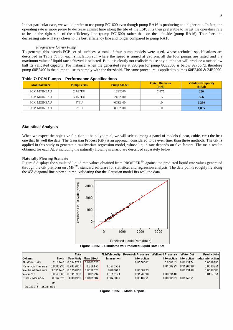
Figure 8 displays the simulated liquid rate values obtained from PROSPERTM
against the predicted liquid rate values generated
through the GP platform on JMPTM
, standard software for statistical and regression analysis. The data points roughly lie along
the 45° diagonal line plotted in red, validating that the Gaussian model fits well the data.
Figure 8: NAT – Simulated vs. Predicted Liquid Rate Plot
Figure 9: NAT – Model Report
9
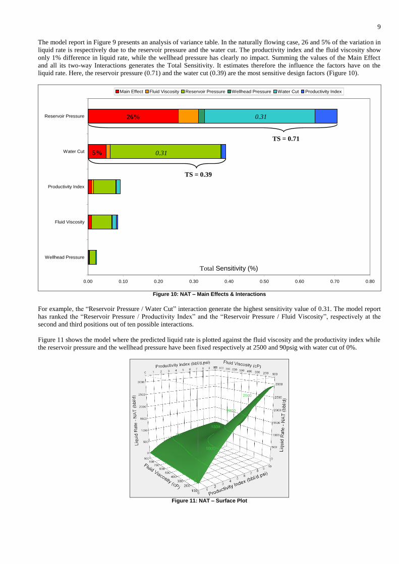
The model report in Figure 9 presents an analysis of variance table. In the naturally flowing case, 26 and 5% of the variation in
liquid rate is respectively due to the reservoir pressure and the water cut. The productivity index and the fluid viscosity show
only 1% difference in liquid rate, while the wellhead pressure has clearly no impact. Summing the values of the Main Effect
and all its two-way Interactions generates the Total Sensitivity. It estimates therefore the influence the factors have on the
liquid rate. Here, the reservoir pressure (0.71) and the water cut (0.39) are the most sensitive design factors (Figure 10).
0.00 0.10 0.20 0.30 0.40 0.50 0.60 0.70 0.80
Wellhead Pressure
Fluid Viscosity
Productivity Index
Water Cut
Reservoir Pressure
Main Effect Fluid Viscosity Reservoir Pressure Wellhead Pressure Water Cut Productivity Index
Figure 10: NAT – Main Effects & Interactions
For example, the “Reservoir Pressure / Water Cut” interaction generate the highest sensitivity value of 0.31. The model report
has ranked the “Reservoir Pressure / Productivity Index” and the “Reservoir Pressure / Fluid Viscosity”, respectively at the
second and third positions out of ten possible interactions.
Figure 11 shows the model where the predicted liquid rate is plotted against the fluid viscosity and the productivity index while
the reservoir pressure and the wellhead pressure have been fixed respectively at 2500 and 90psig with water cut of 0%.
Figure 11: NAT – Surface Plot
26%
5%
TS = 0.71
TS = 0.39
0.31
0.31
Total Sensitivity (%)
10
Electrical Submersible Pump
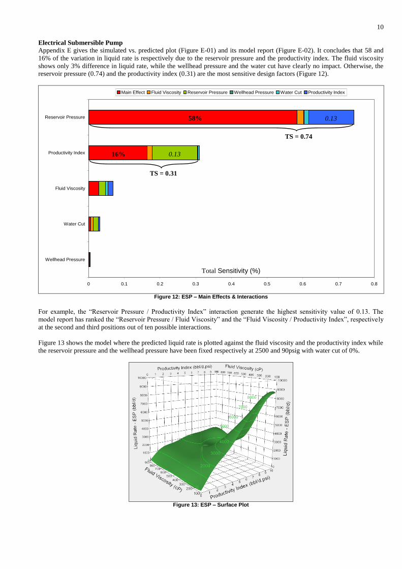
Appendix E gives the simulated vs. predicted plot (Figure E-01) and its model report (Figure E-02). It concludes that 58 and
16% of the variation in liquid rate is respectively due to the reservoir pressure and the productivity index. The fluid viscosity
shows only 3% difference in liquid rate, while the wellhead pressure and the water cut have clearly no impact. Otherwise, the
reservoir pressure (0.74) and the productivity index (0.31) are the most sensitive design factors (Figure 12).
0 0.1 0.2 0.3 0.4 0.5 0.6 0.7 0.8
Wellhead Pressure
Water Cut
Fluid Viscosity
Productivity Index
Reservoir Pressure
Main Effect Fluid Viscosity Reservoir Pressure Wellhead Pressure Water Cut Productivity Index
Figure 12: ESP – Main Effects & Interactions
For example, the “Reservoir Pressure / Productivity Index” interaction generate the highest sensitivity value of 0.13. The
model report has ranked the “Reservoir Pressure / Fluid Viscosity” and the “Fluid Viscosity / Productivity Index”, respectively
at the second and third positions out of ten possible interactions.
Figure 13 shows the model where the predicted liquid rate is plotted against the fluid viscosity and the productivity index while
the reservoir pressure and the wellhead pressure have been fixed respectively at 2500 and 90psig with water cut of 0%.
Figure 13: ESP – Surface Plot
58%
16%
TS = 0.74
TS = 0.31
0.13
0.13
Total Sensitivity (%)
11
Progressive Cavity Pump
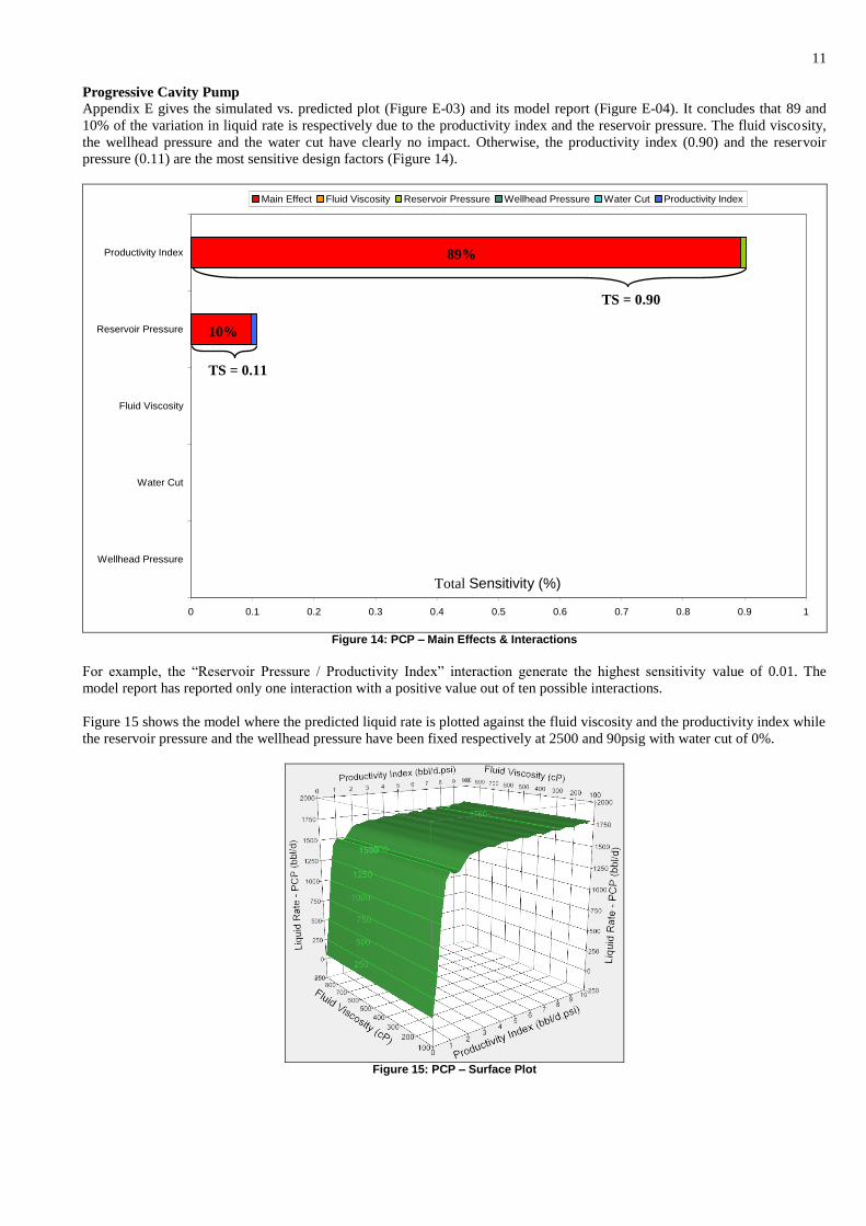
Appendix E gives the simulated vs. predicted plot (Figure E-03) and its model report (Figure E-04). It concludes that 89 and
10% of the variation in liquid rate is respectively due to the productivity index and the reservoir pressure. The fluid viscosity,
the wellhead pressure and the water cut have clearly no impact. Otherwise, the productivity index (0.90) and the reservoir
pressure (0.11) are the most sensitive design factors (Figure 14).
0 0.1 0.2 0.3 0.4 0.5 0.6 0.7 0.8 0.9 1
Wellhead Pressure
Water Cut
Fluid Viscosity
Reservoir Pressure
Productivity Index
Main Effect Fluid Viscosity Reservoir Pressure Wellhead Pressure Water Cut Productivity Index
Figure 14: PCP – Main Effects & Interactions
For example, the “Reservoir Pressure / Productivity Index” interaction generate the highest sensitivity value of 0.01. The
model report has reported only one interaction with a positive value out of ten possible interactions.
Figure 15 shows the model where the predicted liquid rate is plotted against the fluid viscosity and the productivity index while
the reservoir pressure and the wellhead pressure have been fixed respectively at 2500 and 90psig with water cut of 0%.
Figure 15: PCP – Surface Plot
89%
10%
TS = 0.90
TS = 0.11
Total Sensitivity (%)
12
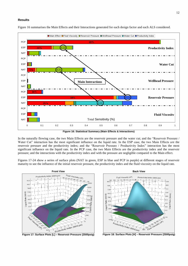
Results
Figure 16 summarises the Main Effects and their Interactions generated for each design factor and each ALS considered.
0 0.1 0.2 0.3 0.4 0.5 0.6 0.7 0.8 0.9 1
NAT
ESP
PCP
NAT
ESP
PCP
NAT
ESP
PCP
NAT
ESP
PCP
NAT
ESP
PCP
Main Effect Fluid Viscosity Reservoir Pressure Wellhead Pressure Water Cut Productivity Index
Figure 16: Statistical Summary (Main Effects & Interactions)
In the naturally flowing case, the two Main Effects are the reservoir pressure and the water cut; and the “Reservoir Pressure /
Water Cut” interaction has the most significant influence on the liquid rate. In the ESP case, the two Main Effects are the
reservoir pressure and the productivity index; and the “Reservoir Pressure / Productivity Index” interaction has the most
significant influence on the liquid rate. In the PCP case, the two Main Effects are the productivity index and the reservoir
pressure; and the interactions with the productivity index and with the pressure are negligible compared to the Main effect.
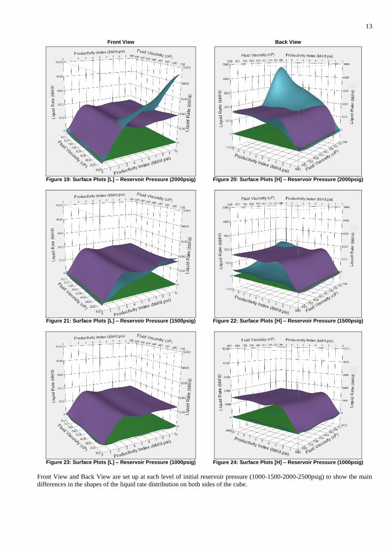
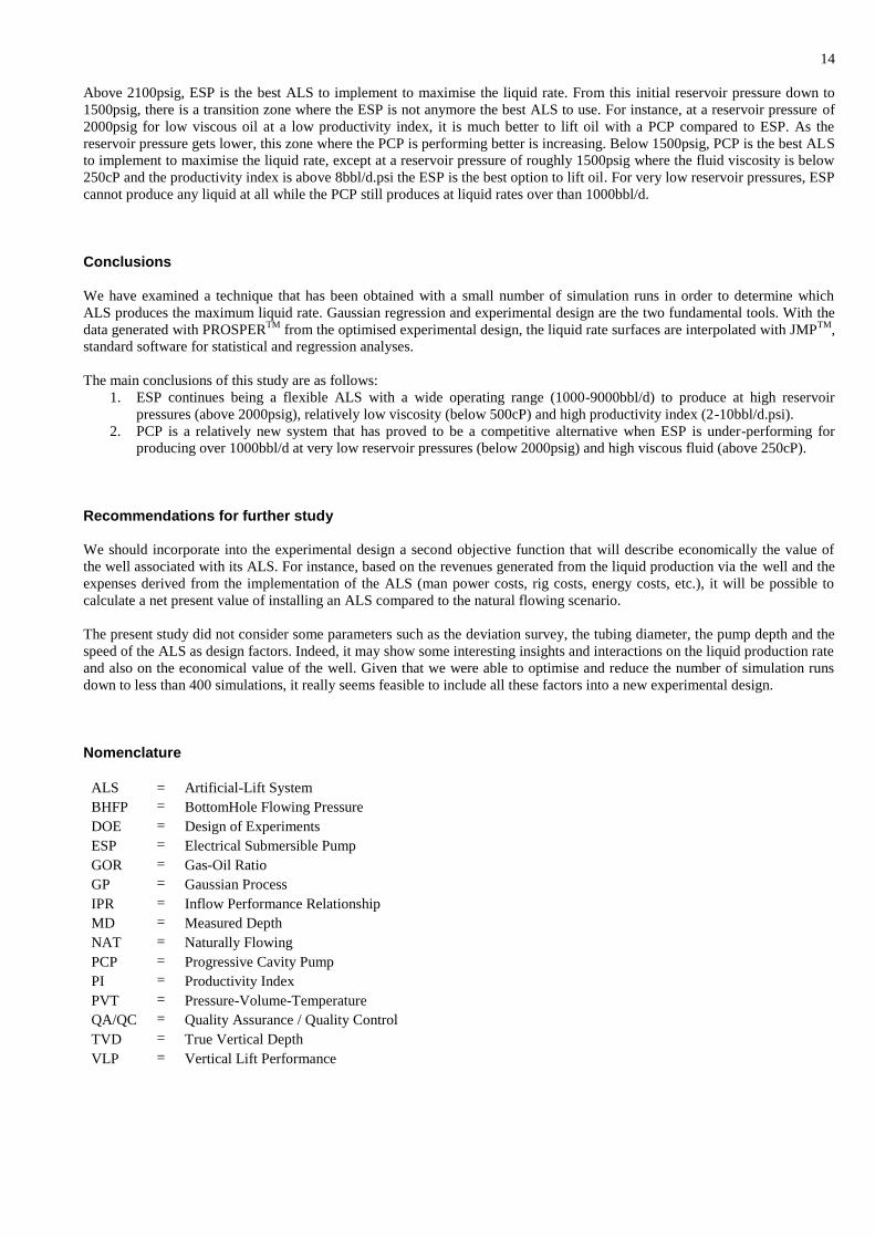
Figures 17-24 show a series of surface plots (NAT in green, ESP in blue and PCP in purple) at different stages of reservoir
maturity to see the influence of the initial reservoir pressure, the productivity index and the fluid viscosity on the liquid rate.
Front View Back View
Figure 17: Surface Plots [L] – Reservoir Pressure (2500psig)
Figure 18: Surface Plots [H] – Reservoir Pressure (2500psig)
Fluid Viscosity
Reservoir Pressure
Wellhead Pressure
Water Cut
Productivity Index
26%
5%
0.31
0.31
58%
16% 0.13
0.13
89%
10%
Main Interactions
Total Sensitivity (%)
13
Front View Back View
Figure 19: Surface Plots [L] – Reservoir Pressure (2000psig)
Figure 20: Surface Plots [H] – Reservoir Pressure (2000psig)
Figure 21: Surface Plots [L] – Reservoir Pressure (1500psig)
Figure 22: Surface Plots [H] – Reservoir Pressure (1500psig)
Figure 23: Surface Plots [L] – Reservoir Pressure (1000psig)
Figure 24: Surface Plots [H] – Reservoir Pressure (1000psig)
Front View and Back View are set up at each level of initial reservoir pressure (1000-1500-2000-2500psig) to show the main
differences in the shapes of the liquid rate distribution on both sides of the cube.
14
Above 2100psig, ESP is the best ALS to implement to maximise the liquid rate. From this initial reservoir pressure down to
1500psig, there is a transition zone where the ESP is not anymore the best ALS to use. For instance, at a reservoir pressure of
2000psig for low viscous oil at a low productivity index, it is much better to lift oil with a PCP compared to ESP. As the
reservoir pressure gets lower, this zone where the PCP is performing better is increasing. Below 1500psig, PCP is the best ALS
to implement to maximise the liquid rate, except at a reservoir pressure of roughly 1500psig where the fluid viscosity is below
250cP and the productivity index is above 8bbl/d.psi the ESP is the best option to lift oil. For very low reservoir pressures, ESP
cannot produce any liquid at all while the PCP still produces at liquid rates over than 1000bbl/d.
Conclusions
We have examined a technique that has been obtained with a small number of simulation runs in order to determine which
ALS produces the maximum liquid rate. Gaussian regression and experimental design are the two fundamental tools. With the
data generated with PROSPERTM
from the optimised experimental design, the liquid rate surfaces are interpolated with JMPTM
,
standard software for statistical and regression analyses.
The main conclusions of this study are as follows:
1. ESP continues being a flexible ALS with a wide operating range (1000-9000bbl/d) to produce at high reservoir
pressures (above 2000psig), relatively low viscosity (below 500cP) and high productivity index (2-10bbl/d.psi).
2. PCP is a relatively new system that has proved to be a competitive alternative when ESP is under-performing for
producing over 1000bbl/d at very low reservoir pressures (below 2000psig) and high viscous fluid (above 250cP).
Recommendations for further study
We should incorporate into the experimental design a second objective function that will describe economically the value of
the well associated with its ALS. For instance, based on the revenues generated from the liquid production via the well and the
expenses derived from the implementation of the ALS (man power costs, rig costs, energy costs, etc.), it will be possible to
calculate a net present value of installing an ALS compared to the natural flowing scenario.
The present study did not consider some parameters such as the deviation survey, the tubing diameter, the pump depth and the
speed of the ALS as design factors. Indeed, it may show some interesting insights and interactions on the liquid production rate
and also on the economical value of the well. Given that we were able to optimise and reduce the number of simulation runs
down to less than 400 simulations, it really seems feasible to include all these factors into a new experimental design.
Nomenclature
ALS = Artificial-Lift System
BHFP = BottomHole Flowing Pressure
DOE = Design of Experiments
ESP = Electrical Submersible Pump
GOR = Gas-Oil Ratio
GP = Gaussian Process
IPR = Inflow Performance Relationship
MD = Measured Depth
NAT = Naturally Flowing
PCP = Progressive Cavity Pump
PI = Productivity Index
PVT = Pressure-Volume-Temperature
QA/QC = Quality Assurance / Quality Control
TVD = True Vertical Depth
VLP = Vertical Lift Performance
15
SI Metric Conversion Factor
bbl × 0.158 987 E+01 = m3
ft × 0.3048 E+00 = m
in 0.2540 E+01 = cm
°F × (°F-32)/1.8 = °C
mD × 0.986 923 E-15 = m2
cP × E+03 = Pa.s
psi × 6.894 757 E-03 = MPa
References
Beal, C.: “The Viscosity of Air, Water, Natural Gas, Crude Oil and Its associated Gases at Oil Field Temperatures and Pressures”, Trans.,
AIME (1946) 165, 94-115.
Standing, M.B.: “A Pressure-Volume-Temperature Correlation for Mixtures of California Oil and Gases”, Drill. and Prod. Prac., API
(1947)275-86.
Lasater, J.A.: “Bubble Point Pressure Correlation”, Trans., AIME (1958) 213, 379-81.
Beggs, H.D. and Robinson, J.R.: “Estimating the Viscosity of Crude Oil Systems”, J. Pet. Tech. (Sept. 1975) 1140-41.
Glaso, O.: “Generalized Pressure-Volume-Temperature Correlations”, J. Pet. Tech. (May 1980) 785-95.
Vasquez, M. and Beggs, H.D.: “Correlations for Fluid Physical Property Prediction”, J. Pet. Tech. (June 1980) 968-70.
Ng, J.T.H. and Egbogah, E.O.: “An Improved Temperature-Viscosity Correlation for Crude Oil Systems”, paper CIM 83-34-32 presented at
the 1983 Petroleum Soc. of CIM Annual Technical Meeting, Banff, May 10-13.
Al-Marhoun, M.A.: “PVT Correlations for Middle East Crude Oils”, J. Pet. Tech. (May 1988) 650-66.
Damsleth, E., Hage, A. and Volden, R.: “Maximum Information at Minimum Cost: A North Sea Field Development Study With an
Experimental Design”, J. Pet. Tech. (Dec. 1992) 1350-56.
Petrosky, Jr. and Farshad, F.F.: “Pressure-Volume-Temperature Correlations for Gulf of Mexico Crude Oils”, paper SPE 26644 presented at
the 1993 Annual Technical Conference and Exhibition, Houston, October 3-6.
Petrosky, Jr. and Farshad, F.F.: “Viscosity Correlations for Gulf of Mexico Oils”, paper SPE 29468 presented at the 1995 Production
Operations Symposium, Oklahoma City, April 2-4.
Belonin, M.D. and Slavin, W.I.: “Abnormally High Formation pressures in petroleum Regions of Russia and Other Countries of the C.I.S.”,
Am. Assoc. Pet. Geol. Mem., (1998) 70, 115-21.
Montgomery, D.C.: Design and Analysis of Experiments, sixth edition, John Wiley & Sons, New York City (2005).
Bergman, D.F. and Sutton, R.P.: “An Update to Viscosity Correlations for Gas-Saturated Crude Oils”, paper SPE 110195 presented at the
2007 SPE Annual Technical Conference and Exhibition, Anaheim, Nov. 11-14.
Parfenov, A.N., Sitdikov, S.S., Evseev, O.V., Shashel, V.A. and Butula, K.K.: “Particularities in Hydraulic Fracturing in Dome Type
Reservoirs of Samara Area in the Volga Urals Basin”, paper SPE 115556 presented at the 2008 SPE Russian Oil &Gas Technical Conference
and Exhibition, Moscow, Oct. 28-30.
16
Appendices
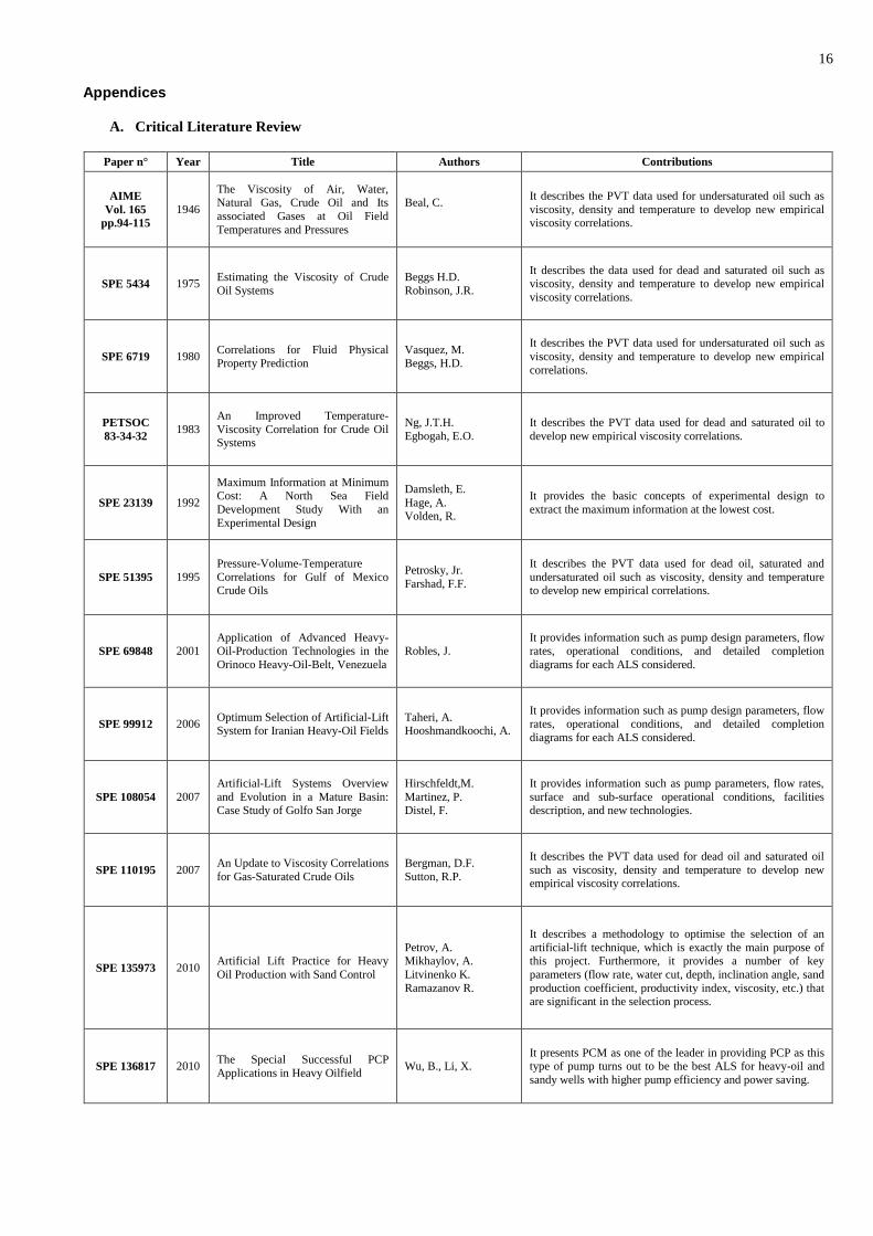
A. Critical Literature Review
Paper n° Year Title Authors Contributions
AIME
Vol. 165
pp.94-115
1946
The Viscosity of Air, Water, Natural Gas, Crude Oil and Its
associated Gases at Oil Field
Temperatures and Pressures
Beal, C.
It describes the PVT data used for undersaturated oil such as
viscosity, density and temperature to develop new empirical viscosity correlations.
SPE 5434 1975 Estimating the Viscosity of Crude
Oil Systems
Beggs H.D.
Robinson, J.R.
It describes the data used for dead and saturated oil such as viscosity, density and temperature to develop new empirical
viscosity correlations.
SPE 6719 1980 Correlations for Fluid Physical
Property Prediction
Vasquez, M.
Beggs, H.D.
It describes the PVT data used for undersaturated oil such as
viscosity, density and temperature to develop new empirical
correlations.
PETSOC
83-34-32 1983
An Improved Temperature-
Viscosity Correlation for Crude Oil Systems
Ng, J.T.H.
Egbogah, E.O.
It describes the PVT data used for dead and saturated oil to
develop new empirical viscosity correlations.
SPE 23139 1992
Maximum Information at Minimum Cost: A North Sea Field
Development Study With an
Experimental Design
Damsleth, E.
Hage, A. Volden, R.
It provides the basic concepts of experimental design to
extract the maximum information at the lowest cost.
SPE 51395 1995
Pressure-Volume-Temperature
Correlations for Gulf of Mexico Crude Oils
Petrosky, Jr.
Farshad, F.F.
It describes the PVT data used for dead oil, saturated and
undersaturated oil such as viscosity, density and temperature to develop new empirical correlations.
SPE 69848 2001 Application of Advanced Heavy-Oil-Production Technologies in the
Orinoco Heavy-Oil-Belt, Venezuela
Robles, J. It provides information such as pump design parameters, flow rates, operational conditions, and detailed completion
diagrams for each ALS considered.
SPE 99912 2006 Optimum Selection of Artificial-Lift System for Iranian Heavy-Oil Fields
Taheri, A. Hooshmandkoochi, A.
It provides information such as pump design parameters, flow
rates, operational conditions, and detailed completion
diagrams for each ALS considered.
SPE 108054 2007
Artificial-Lift Systems Overview
and Evolution in a Mature Basin: Case Study of Golfo San Jorge
Hirschfeldt,M.
Martinez, P. Distel, F.
It provides information such as pump parameters, flow rates,
surface and sub-surface operational conditions, facilities description, and new technologies.
SPE 110195 2007 An Update to Viscosity Correlations
for Gas-Saturated Crude Oils
Bergman, D.F.
Sutton, R.P.
It describes the PVT data used for dead oil and saturated oil
such as viscosity, density and temperature to develop new empirical viscosity correlations.
SPE 135973 2010 Artificial Lift Practice for Heavy
Oil Production with Sand Control
Petrov, A. Mikhaylov, A.
Litvinenko K.
Ramazanov R.
It describes a methodology to optimise the selection of an
artificial-lift technique, which is exactly the main purpose of this project. Furthermore, it provides a number of key
parameters (flow rate, water cut, depth, inclination angle, sand
production coefficient, productivity index, viscosity, etc.) that are significant in the selection process.
SPE 136817 2010 The Special Successful PCP
Applications in Heavy Oilfield Wu, B., Li, X.
It presents PCM as one of the leader in providing PCP as this type of pump turns out to be the best ALS for heavy-oil and
sandy wells with higher pump efficiency and power saving.

17
AIME Vol. 165 pp.94-115 (1946)
The Viscosity of Air, Water, Natural Gas, Crude Oil and Its associated Gases at Oil Field Temperatures and Pressures
Authors: Beal, C.
Contribution to the selection of viscosity correlations:
Medium. The paper describes the PVT data used for undersaturated oil such as viscosity, density and temperature to develop
new empirical viscosity correlations. Then, it enables me to quality-check if the heavy-oil reservoirs in Samara can be
modelled by the Beal correlation.
Objective of the paper:
This paper plays with a large database of laboratory measured data from fields all over the world to produce empirical
correlations. It summarises graphically published correlations of the viscosity of air, water and natural gases. Where it was
possible, correlations were derived to encompass a wide range of temperature and pressure experienced in oil fields.
Methodology used:
52 viscosity data points taken from 26 crude oil samples were analysed to develop the charts and correlations. The first half of
the data set includes viscosity observations taken above the bubble point, while the other half were taken at the bubble point.
Conclusions reached:
1. Being in possession of only the oil density, initial gas-oil ratio, and temperature and pressure at reservoir conditions,
the Beal correlation is likely to forecast the oil viscosity with a 19.8% of deviation.
2. When estimating outside of the range of data used to derive the correlations, caution should be exercised.
Comments:
The correlations do consider undersaturated oil.

18
SPE 5434 (1975)
Estimating the Viscosity of Crude Oil Systems
Authors: Beggs H.D., Robinson, J.R.
Contribution to the selection of viscosity correlations:
Medium. The paper describes the data used for dead and saturated oil such as viscosity, density and temperature to develop
new empirical viscosity correlations. Then, it enables me to quality-check if the heavy-oil reservoirs in Samara can be
modelled by the Beggs correlation.
Objective of the paper:
This paper plays with a large database of laboratory measured PVT data from fields all over the world to produce newly
improved empirical viscosity correlations. This would substitute those commonly in use and enlarge its range of applicability.
Methodology used:
The study accumulates more than 600 laboratory PVT analyses from fields all over the world. The data covered very wide
ranges of reservoir properties and included more than 6,000 measurements of Rs, Bo and μo at various pressures.
Conclusions reached:
1. The correlations give a fair viscosity estimate over a wide range of oil density and reservoir temperature.
2. When estimating outside of the range of data used to derive the correlations, caution should be exercised.
Comments:
The correlations do not consider undersaturated oil.

19
SPE 6719 (1980)
Correlations for Fluid Physical Property Prediction
Authors: Vasquez, M., Beggs, H.D.
Contribution to the selection of viscosity correlations:
Medium. The paper describes the PVT data used for undersaturated oil such as viscosity, density and temperature to develop
new empirical correlations. Then, it enables me to quality-check if the heavy-oil reservoirs in Samara can be modelled by the
Vasquez-Beggs correlation.
Objective of the paper:
This paper plays with a large database of laboratory measured PVT data from fields all over the world to produce improved
empirical correlations. This would substitute those commonly in use and enlarge its range of applicability.
Methodology used:
The study accumulates more than 600 laboratory PVT analyses from fields all over the world. The data covered very wide
ranges of reservoir properties and included more than 6,000 measurements of Rs, Bo and μo at various pressures.
Conclusions reached:
1. Improved empirical correlations have been developed for the most relevant oil properties (density, Bo, viscosity).
2. A much larger database was studied here; therefore, the results should be applicable to a wider range of oil properties.
3. When estimating outside of the range of data used to derive the correlations, caution should be exercised.
Comments:
The correlations do consider undersaturated oil.

20
PETSOC 93-34-32 (1983)
An Improved Temperature-Viscosity Correlation for Crude Oil Systems
Authors: Ng, J.T.H. and Egbogah, E.O.
Contribution to the selection of viscosity correlations:
Medium. The paper describes the PVT data used for dead and saturated oil to develop new empirical viscosity correlations.
Then, it enables me to quality-check if the heavy-oil reservoirs in Samara can be modelled by the Egbogah correlation.
Objective of the paper:
This paper plays with a large database of laboratory measured PVT data from fields all over the world to produce improved
empirical correlations. This would substitute those commonly in use and enlarge its range of applicability. In particular, it
derives a modified Beggs and Robinson empirical viscosity correlation.
Methodology used:
The viscosity database is taken from the Reservoir Fluids Analysis Laboratory of AGAT Engineering Ltd. They accumulated a
total number of 394 oil systems to generate these newly regression equations.
Conclusions reached:
1. The results obtained demonstrate a significant refinement over the original Beggs and Robinson correlation.
2. When estimating outside of the range of data used to derive the correlations, caution should be exercised.
Comments:
The correlations do not consider undersaturated oil. Any range of parameters is provided.

21
SPE 23139 (1992)
Maximum Information at Minimum Cost: A North Sea Field Development Study With an Experimental Design
Authors: Damsleth, E., Hage, A., Voden, R.
Contribution to the experimental design:
High. This paper provides the basic concepts of experimental design. It describes how to construct the settings of each input
parameter in order to extract the maximum information in the fewest amount of runs.
Objective of the paper:
This paper applies the DOE methodology to a real case study from the North Sea to prove that it is possible to maximise the
information acquired from a minimum number of simulations runs. The technique provides additional information about
interactions between input parameters from a few more runs.
Methodology used:
The design procedure is as follows:
1. Select the appropriate regression model for which the design is optimal
2. Identify how many simulations to run for the selected regression model
3. Create a list of possible experiments of input parameters for the design
Conclusions reached:
1. This DOE gives the same information as the one-factor-at-a-time experimentation with 40% fewer simulations runs.
2. The response-surface analysis tool determines and evaluates likely interactions between the various factors.

22
SPE 51395 (1995)
Pressure-Volume-Temperature Correlations for Gulf of Mexico Crude Oils
Authors: Petrosky, Jr., Farshad, F.F.
Contribution to the selection of viscosity correlations:
Medium. The paper describes the PVT data used for dead oil, saturated and undersaturated oil such as viscosity, density and
temperature to develop new empirical viscosity correlations. Then, it enables me to quality-check if the heavy-oil reservoirs in
Samara can be modelled by the Petrosky correlation.
Objective of the paper:
This paper plays with a large database of laboratory measured PVT data from fields all over the world to produce improved
empirical correlations. This would substitute those commonly in use and enlarge its range of applicability.
Methodology used:
A total of 81 laboratory PVT analyses were analysed to derive the new oil viscosity correlations. The data covered very wide
ranges of reservoir properties and included more than 300 measurements of compressibility, temperature, and bubble point.
Conclusions reached:
1. The results obtained demonstrate a significant refinement over the original published correlations.
2. When estimating outside of the range of data used to derive the correlations, caution should be exercised.
Comments:
The correlations do consider undersaturated oil.

23
SPE 69848 (2001)
Application of Advanced Heavy-Oil-Production Technologies in the Orinoco Heavy-Oil-Belt, Venezuela
Authors: Robles, J.
Contribution to the selection of artificial-lift system:
Medium. This paper provides information such as pump design parameters, flow rates, operational conditions, and detailed
completion diagrams for each artificial-lift systems considered. It has brought out enough information to fill out the technical
inputs required to model the panel of artificial-lift systems in PROSPERTM
.
Objective of the paper:
The paper sumarises the latest pump experiences of Petrozuata C.A. in the Zuata field in the use of ESP and PCP.
Methodology used:
Observations are based on surface and sub-surface information.
Conclusions reached:
1. The use of multilateral technology has offered the possibility for Petrozuata to develop high potential wells, issuing
new challenges in terms of lifting higher flow rates.
2. Application of high rate ESP systems has allowed to produce 3,000bopd at moderate intake pressures (>500psig),
while past experiences have showed that lower pump intake pressure and higher GOR (>100scf/stb) can reduce the
global net output of the artificial-lift system by 50%.
Comments:
This paper is dealing with more viscous heavy-oil fields at higher flow rates compared to the Russian ones in Samara.

24
SPE 99912 (2006)
Optimum Selection of Artificial-Lift System for Iranian Heavy-Oil Fields
Authors: Taheri, A., Hooshmandkoochi, A.
Contribution to the optimum selection of artificial-lift system:
Medium. This paper provides information such as pump design parameters, flow rates, operational conditions, and detailed
completion diagrams for each artificial-lift systems considered. It has brought out enough information to fill out the technical
inputs required to model the panel of artificial-lift systems in PROSPERTM
.
Objective of the paper:
This paper describes the screening criteria on a panel of artificial-lift techniques to lift the heavy-oil reservoirs. In fact, it
discusses the technical issues behind each system of artificial-lift for a particular well located in a heavy-oil Iranian reservoir.
The result of the study is to address why the best suitable artificial-lift choice was confined to PCP for this particular well
under examination.
Methodology used:
The selection process was based on technical, economic and environmental considerations.
Conclusions reached:
1. ESP can not be optimised because of no stable intersection between the inflow and outflow performance curves.
2. Gas lift can not be applied here for a non-technical reason as there is no close gas source around the well.
3. PCP seems to be the best suitable technique because of a high oil specific gravity and a low reservoir pressure.
4. Because of a low pressure reservoir, the HJP was not appropriate to optimise the output for this particular well.
Comments:
This paper is dealing with a very different heavy-oil reservoir compared to the Russian ones in Samara.

25
SPE 108054 (2007)
Artificial-Lift Systems Overview and Evolution in a Mature Basin: Case Study of Golfo San Jorge
Authors: Hirschfeldt, M., Martinez, P., Distel, F.
Contribution to the selection of artificial-lift system:
High. This paper provides information such as pump parameters, flow rates, surface and sub-surface operational conditions,
facilities description, breakdowns statistics, and new technologies. It has brought out enough information to fill out the
technical inputs required to model the panel of artificial-lift systems in PROSPERTM
.
Objective of the paper:
The result of the overview is to provide an artificial-lift system guide, populated with technical parameters and in-house
benchmarks associated with a broad range of operational information from more than 9,000 active wells from different
oilfields. The paper describes the selection and the optimisation of several artificial-lift systems (PCP, ESP, and SRP).
Furthermore, a basic description and operational applications to some oilfields about gas lift, plunger lift and hydraulic jet
pump practices is also provided at the end.
Methodology used:
Observations are based on surface and sub-surface information.
Conclusions reached:
1. SRP, PCP and ESP are the most popular systems used for producing more than 90% of the fluid of the onshore basin.
2. PCP started as a cost-efficient alternative for low flow rate, heavy oil and sand production. But as it is a new
technology, its breakdown index is bigger compared to the other pumps such as SRP and ESP.
3. Operating the ESP below perforations achieved a successful outcome in this multi-layered reservoir. Also, the high
reliability of “plug-and-play” ESP system seems to become a promising practice.
4. Hydraulic jet pump is most used for its efficiency to produce wells with severity problems and sand production.
Comments:
This paper is dealing with more viscous heavy-oil fields at higher flow rates compared to the Russian ones in Samara.

26
SPE 110195 (2007)
An Update to Viscosity Correlations for Gas-Saturated Crude Oils
Authors: Bergman, D.F., Sutton, R.P.
Contribution to the selection of viscosity correlations:
Medium. The paper describes the PVT data used for dead oil and saturated oil such as viscosity, density and temperature to
develop new empirical viscosity correlations. Then, it enables me to quality-check if the heavy-oil reservoirs in Samara can be
modelled by the Bergman-Sutton correlation.
Objective of the paper:
This paper plays with a large database of laboratory measured PVT data from fields all over the world to produce improved
empirical correlations. This would substitute those commonly in use and enlarge its range of applicability.
Methodology used:
A total of 1849 laboratory PVT samples were analysed to derive the new oil viscosity correlations. The data covered very wide
ranges of reservoir properties and included more than 12,000 measurements of Rs and μo at various pressures.
Conclusions reached:
1. The results obtained offer an increased refinement over the existing correlations.
2. When estimating outside of the range of data used to derive the correlations, caution should be exercised.
Comments:
The correlations do not consider undersaturated oil.

27
SPE 135973 (2010)
Artificial Lift Practice for Heavy Oil Production with Sand Control
Authors: Petrov, A., Mikhaylov, A., Litvinenko K., Ramazanov R.
Contribution to the selection of artificial-lift system:
High. This paper describes a methodology to optimise the selection of an artificial-lift technique, which is exactly the main
purpose of this project. Furthermore, it provides a number of key parameters (flow rate, water cut, depth, inclination angle,
sand production coefficient, productivity index, viscosity, etc.) that are significant in the selection process and need to be taken
into account in this study.
Objective of the paper:
This paper develops and evaluates a new algorithm to be used for optimising the selection process of a panel of artificial-lift
techniques to lift heavy-oil reservoirs where the sand production is an issue.
The procedure is falling into three main steps:
1. Build a database of recommendations to gathering practical experiences of a range of artificial lift techniques, whose
technology is classified to three levels of application (unrecommended, applicable and recommended).
2. Create a method to select the most suitable artificial-lift systems out of short-listed techniques relevant to a heavy-oil
field development plan with sand production by the application of a Matrix of Technologies.
3. Assess the effectiveness of the Matrix of Technologies on a real case study (North Komsomolskoe Russian field) to
ensure the conclusions are consistent between the study and the testing operations.
Methodology used:
The selection process is divided into two stages:
1. Matrix of artificial lift technologies is constructed, only based on practices relevant for operating heavy-oil fields with
sand control. The first result was to short-list two pumps out the five for a more detailed study;
2. Matrix of artificial lift technologies is built based on the pump performances in terms of oil production for a given
range of PI and viscosity to map the boundary where it will be best to implement either the PCP or the HJP.
Conclusions reached:
1. In the range of oil viscosity in the North Komsmolkoye field (50-500cP), the Matrix has selected HJP and PCP as the
best ones. Applying this method enables to build maps of applicability for new parameters like the GOR.
2. At the stage of testing technology, the PCP has been selected as the most effective pump to target the highest likely
production in terms of implementation in the North Komsomolskoye field.
Comments:
The case study is similar to the heavy-oil reservoirs in Samara, except the fact that there is no issue of sand production. The
essence of the method to select the best ALS is only based on two key parameters (productivity index and viscosity) while the
project will encompass more drivers such as the reservoir pressure, the water cut and some pump parameters.

28
SPE 136817 (2010)
The Special Successful PCP Applications in Heavy Oilfield
Authors: Wu, B., Li, X.
Contribution to the selection of artificial-lift system:
Medium. This paper presents PCM as one of the leader in providing PCP as this type of pump turns out to be the best ALS for
heavy-oil and sandy wells with higher pump efficiency and power saving.
Objective of the paper:
This paper describes in details the successful applications of 5 specific PCP systems (PCM VulcainTM
, PCM 198 High
Temperature Elastomer, PCM new technologies with light oil injection, with hot water injection and with electrical heating). It
provides information such as pump design parameters, flow rates, operational conditions, detailed completion diagrams, and
failures statistics for each PCP system considered.
Methodology used:
Each artificial-lift system is presented separately.
Conclusion reached:
1. These favourable applications have truly demonstrated the feasibility and success of PCP in heavy-oil production.
2. These 5 specific PCP new technologies have enlarged the application range of the successful conventional PCP.
Comments:
I have contacted PCM France to obtain a set of PCP performance curves.
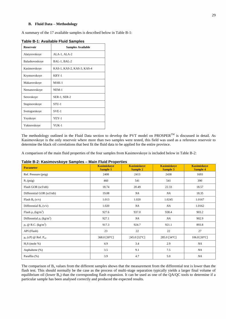
29
B. Fluid Data – Methodology
A summary of the 17 available samples is described below in Table B-1:
Table B-1: Available Fluid Samples
Reservoir Samples Available
Alatyrovskoye ALA-1, ALA-2
Balashovoskoye BAL-1, BAL-2
Kasimovskoye KAS-1, KAS-2, KAS-3, KAS-4
Krymsovskoye KRY-1
Makarovskoye MAK-1
Nemanovskoye NEM-1
Serovskoye SER-1, SER-2
Stupinovskoye STU-1
Svetogorskoye SVE-1
Yeyskoye YEY-1
Yuknovskoye YUK-1
The methodology outlined in the Fluid Data section to develop the PVT model on PROSPERTM
is discussed in detail. As
Kasimovskoye is the only reservoir where more than two samples were tested, this field was used as a reference reservoir to
determine the black oil correlations that best fit the fluid data to be applied for the entire province.
A comparison of the main fluid properties of the four samples from Kasimovskoye is included below in Table B-2:
Table B-2: Kasimovskoye Samples – Main Fluid Properties
Parameter Kasimiskoye
Sample 1
Kasimiskoye
Sample 2
Kasimiskoye
Sample 3
Kasimiskoye
Sample 4
Ref. Pressure (psig) 2408 2413 2438 1693
Pb (psig) 460 541 541 390
Flash GOR (scf/stb) 18.74 20.49 22.33 18.57
Differential GOR (scf/stb) 19.08 NA NA 18.35
Flash Bo (v/v) 1.013 1.020 1.0245 1.0167
Differential Bo (v/v) 1.020 NA NA 1.0162
Flash ρo (kg/m3) 927.6 937.0 938.4 903.2
Differential ρo (kg/m3) 927.1 NA NA 902.9
ρo @ R.C. (kg/m3) 917.3 924.7 921.1 893.8
API (Flash) 23 22 22 27
μo (cP) @ Ref. Pref 368.0 [30°C] 245.0 [32°C] 285.0 [34°C] 106.8 [30°C]
H2S (mole %) 4.9 3.4 2.9 NA
Asphaltene (%) 3.5 9.1 7.5 NA
Paraffin (%) 3.9 4.7 5.0 NA
The comparison of Bo values from the different samples shows that the measurement from the differential test is lower than the
flash test. This should normally be the case as the process of multi-stage separation typically yields a larger final volume of
equilibrium oil (lower Bo) than the corresponding flash expansion. It can be used as one of the QA/QC tools to determine if a
particular sample has been analysed correctly and produced the expected results.
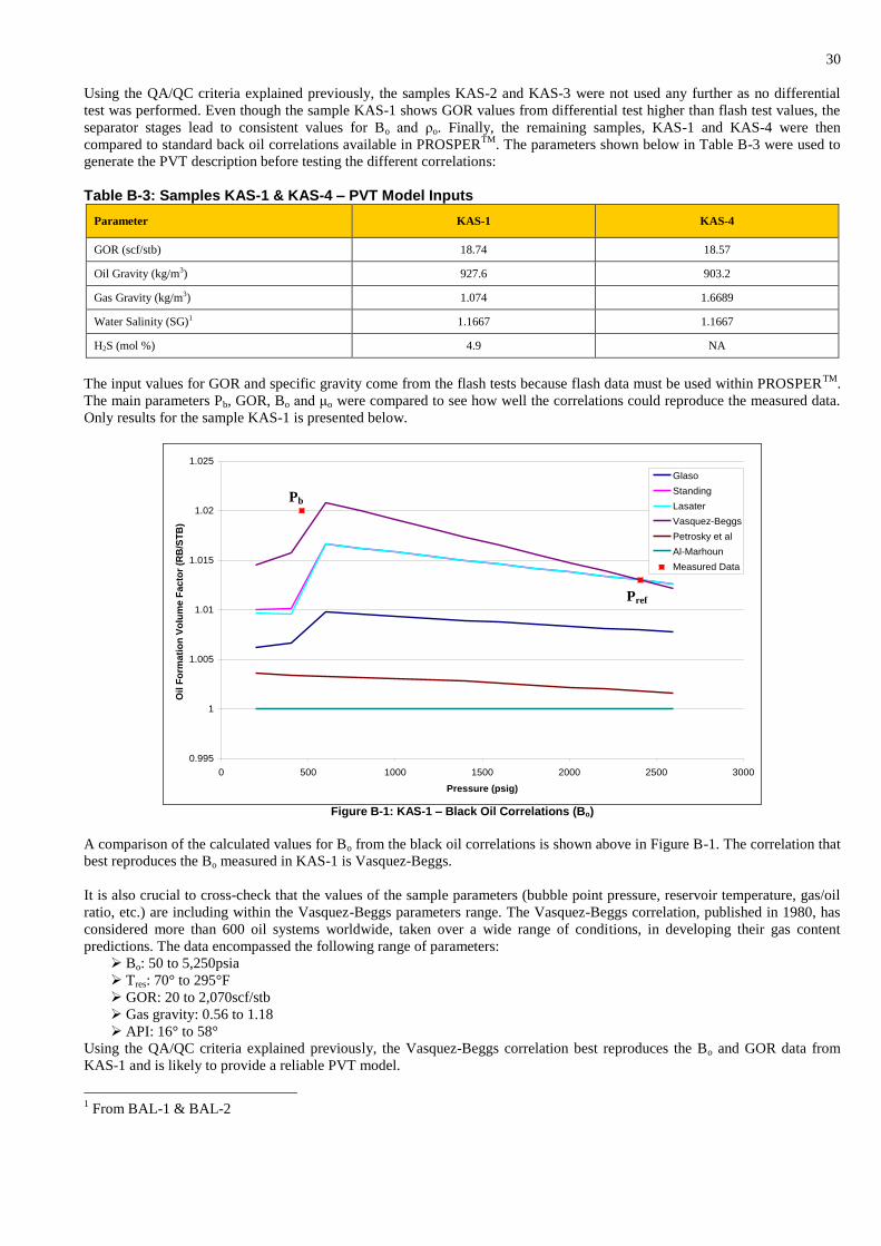
30
Using the QA/QC criteria explained previously, the samples KAS-2 and KAS-3 were not used any further as no differential
test was performed. Even though the sample KAS-1 shows GOR values from differential test higher than flash test values, the
separator stages lead to consistent values for Bo and ρo. Finally, the remaining samples, KAS-1 and KAS-4 were then
compared to standard back oil correlations available in PROSPERTM
. The parameters shown below in Table B-3 were used to
generate the PVT description before testing the different correlations:
Table B-3: Samples KAS-1 & KAS-4 – PVT Model Inputs
Parameter KAS-1 KAS-4
GOR (scf/stb) 18.74 18.57
Oil Gravity (kg/m3) 927.6 903.2
Gas Gravity (kg/m3) 1.074 1.6689
Water Salinity (SG)1 1.1667 1.1667
H2S (mol %) 4.9 NA
The input values for GOR and specific gravity come from the flash tests because flash data must be used within PROSPERTM
.
The main parameters Pb, GOR, Bo and μo were compared to see how well the correlations could reproduce the measured data.
Only results for the sample KAS-1 is presented below.
0.995
1
1.005
1.01
1.015
1.02
1.025
0 500 1000 1500 2000 2500 3000
Pressure (psig)
Oil
Fo
rma
tio
n V
olu
me
Fa
cto
r (R
B/S
TB
)
Glaso
Standing
Lasater
Vasquez-Beggs
Petrosky et al
Al-Marhoun
Measured Data
Figure B-1: KAS-1 – Black Oil Correlations (Bo)
A comparison of the calculated values for Bo from the black oil correlations is shown above in Figure B-1. The correlation that
best reproduces the Bo measured in KAS-1 is Vasquez-Beggs.
It is also crucial to cross-check that the values of the sample parameters (bubble point pressure, reservoir temperature, gas/oil
ratio, etc.) are including within the Vasquez-Beggs parameters range. The Vasquez-Beggs correlation, published in 1980, has
considered more than 600 oil systems worldwide, taken over a wide range of conditions, in developing their gas content
predictions. The data encompassed the following range of parameters:
Bo: 50 to 5,250psia
Tres: 70° to 295°F
GOR: 20 to 2,070scf/stb
Gas gravity: 0.56 to 1.18
API: 16° to 58°
Using the QA/QC criteria explained previously, the Vasquez-Beggs correlation best reproduces the Bo and GOR data from
KAS-1 and is likely to provide a reliable PVT model.
1 From BAL-1 & BAL-2
Pb
Pref
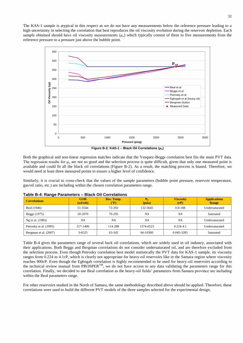
31
The KAS-1 sample is atypical in this respect as we do not have any measurements below the reference pressure leading to a
high uncertainty in selecting the correlation that best reproduces the oil viscosity evolution during the reservoir depletion. Each
sample obtained should have oil viscosity measurements (μo) which typically consist of three to five measurements from the
reference pressure to a pressure just above the bubble point.
0
50
100
150
200
250
300
350
400
450
0 500 1000 1500 2000 2500 3000
Pressure (psig)
Oil
Vis
co
sit
y (
cp
)
Beal et al
Beggs et al
Petrosky et al
Egbogah et al (heavy oil)
Bergman-Sutton
Measured Data
Figure B-2: KAS-1 – Black Oil Correlations (μo)
Both the graphical and non-linear regression matches indicate that the Vasquez-Beggs correlation best fits the main PVT data.
The regression results for μo are not so good and the selection process is quite difficult, given that only one measured point is
available and could fit all the black oil correlations (Figure B-2). As a result, the matching process is biased. Therefore, we
would need at least three measured points to ensure a higher level of confidence.
Similarly, it is crucial to cross-check that the values of the sample parameters (bubble point pressure, reservoir temperature,
gas/oil ratio, etc.) are including within the chosen correlation parameters range.
Table B-4: Range Parameters – Black Oil Correlations
Correlations GOR
(scf/stb)
Res. Temp.
(°F)
Pb
(psia)
Viscosity
(cP)
Applications
Range
Beal (1946) 51-3544 72-292 132-5645 0.8-188 Undersaturated
Beggs (1975) 20-2070 70-295 NA NA Saturated
Ng et al. (1983) NA NA NA NA Undersaturated
Petrosky et al. (1995) 217-1406 114-288 1574-6523 0.224-4.1 Undersaturated
Bergman et al. (2007) 3-6525 63-342 66-10300 0.045-3285 Saturated
Table B-4 gives the parameters range of several back oil correlations, which are widely used in oil industry, associated with
their applications. Both Beggs and Bergman correlations do not consider undersaturated oil, and are therefore excluded from
the selection process. Even though Petrosky correlation best model statistically the PVT data for KAS-1 sample, its viscosity
ranges from 0.224 to 4.1cP, which is clearly not appropriate for heavy-oil reservoirs like in the Samara region where viscosity
reaches 900cP. Even though the Egbogah correlation is highly recommended to be used for heavy-oil reservoirs according to
the technical review manual from PROSPERTM
, we do not have access to any data validating the parameters range for this
correlation. Finally, we decided to use Beal correlation as the heavy-oil fields’ parameters from Samara province are including
within the Beal parameters range.
For other reservoirs studied in the North of Samara, the same methodology described above should be applied. Therefore, these
correlations were used to build the different PVT models of the three samples selected for the experimental design.
Pref
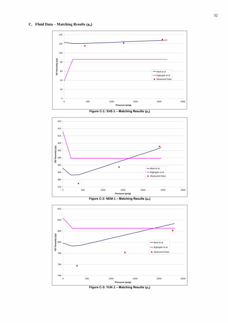
32
C. Fluid Data – Matching Results (μo)
0
20
40
60
80
100
120
140
0 500 1000 1500 2000 2500
Pressure (psig)
Oil V
isc
os
ity
(c
p)
Beal et al
Egbogah et al
Measured Data
Figure C-1: SVE-1 – Matching Results (μo)
375
380
385
390
395
400
405
410
415
420
0 500 1000 1500 2000 2500 3000
Pressure (psig)
Oil V
isc
os
ity
(c
p)
Beal et al
Egbogah et al
Measured Data
Figure C-2: NEM-1 – Matching Results (μo)
785
790
795
800
805
810
815
0 500 1000 1500 2000 2500
Pressure (psig)
Oil
Vis
co
sit
y (
cp
)
Beal et al
Egbogah et al
Measured Data
Figure C-3: YUK-1 – Matching Results (μo)
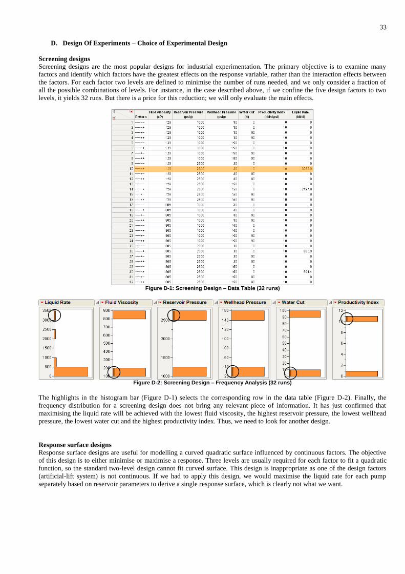
33
D. Design Of Experiments – Choice of Experimental Design
Screening designs
Screening designs are the most popular designs for industrial experimentation. The primary objective is to examine many
factors and identify which factors have the greatest effects on the response variable, rather than the interaction effects between
the factors. For each factor two levels are defined to minimise the number of runs needed, and we only consider a fraction of
all the possible combinations of levels. For instance, in the case described above, if we confine the five design factors to two
levels, it yields 32 runs. But there is a price for this reduction; we will only evaluate the main effects.
Figure D-1: Screening Design – Data Table (32 runs)
Figure D-2: Screening Design – Frequency Analysis (32 runs)
The highlights in the histogram bar (Figure D-1) selects the corresponding row in the data table (Figure D-2). Finally, the
frequency distribution for a screening design does not bring any relevant piece of information. It has just confirmed that
maximising the liquid rate will be achieved with the lowest fluid viscosity, the highest reservoir pressure, the lowest wellhead
pressure, the lowest water cut and the highest productivity index. Thus, we need to look for another design.
Response surface designs
Response surface designs are useful for modelling a curved quadratic surface influenced by continuous factors. The objective
of this design is to either minimise or maximise a response. Three levels are usually required for each factor to fit a quadratic
function, so the standard two-level design cannot fit curved surface. This design is inappropriate as one of the design factors
(artificial-lift system) is not continuous. If we had to apply this design, we would maximise the liquid rate for each pump
separately based on reservoir parameters to derive a single response surface, which is clearly not what we want.
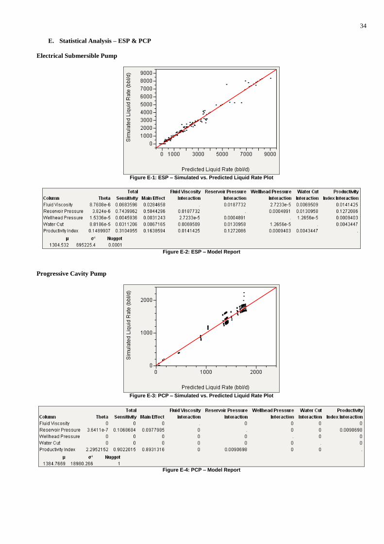
34
E. Statistical Analysis – ESP & PCP
Electrical Submersible Pump
Figure E-1: ESP – Simulated vs. Predicted Liquid Rate Plot
Figure E-2: ESP – Model Report
Progressive Cavity Pump
Figure E-3: PCP – Simulated vs. Predicted Liquid Rate Plot
Figure E-4: PCP – Model Report