Electronic copy available at: http://ssrn.com/abstract=1472002

Option Happiness and Liquidity: Is the Dynamics of the Volatility

Smirk Affected by Relative Option Liquidity?

Lars Nordén1 and Caihong Xu

Finance Department, Stockholm University School of Business,

S-106 91 Stockholm, Sweden

Abstract

This study investigates the dynamic relationship between option happiness (the steepness of the

volatility smirk) and relative index option liquidity. We find that, on a daily basis, option

happiness is significantly dependent on the relative liquidity between option series with different

moneyness. In particular, the larger the difference in liquidity between an out-of-the-money

option and a concurrent at-the-money call option, the larger the option happiness. This

relationship is robust to various relative option liquidity measures based on bid-ask spreads,

trading volumes and option price impacts. The results also show a significant maturity effect in

option happiness, consistent with the notion that options are “dying smiling”.

Key words: Implied volatility; Volatility smirk; Option happiness; Relative option liquidity

1 Lars Nordén is Professor of Finance at Stockholm University School of Business, Sweden. Caihong Xu is a Ph. D.

Candidate at Stockholm University School of Business, Sweden. Please send correspondence to Lars Nordén,

Stockholm University School of Business, S-106 91 Stockholm, Sweden. Phone: + 46 8 6747139; Fax: + 46 8

6747440; E-mail: ln@fek.su.se. Both authors are grateful to the Jan Wallander and Tom Hedelius foundation and the

Tore Browaldh foundation for research support.

Electronic copy available at: http://ssrn.com/abstract=1472002

2

1. Introduction

One of the most absorbing and well-documented puzzles in the options literature is the volatility

smile or smirk, which relates to the commonly observed excess implied volatility (hereafter IV)

of out-of-the-money (OTM) options relative to at-the-money (ATM) options based on the Black-

Scholes (1973) (BS) model.2 In the last three decades, a large number of studies have been

dedicated to explaining the smirk by relaxing some of the restrictive BS assumptions. Substantial

progress has been made, and examples include: 1) the implied binominal tree models of Dupire

(1994) and Rubinstein (1994); 2) the stochastic volatility and stochastic interest rate models of

Amin and Ng (1993), Bakshi and Chen (1997); and 3) the stochastic volatility jump-diffusion

models of Bates (2000), and Scott (1997).3 However, empirical studies by Bakshi et al. (1997),

Bates (2000), and Dumas et al. (1998) indicate that even the most flexible option pricing models

fail to fully capture the dynamics of the volatility smirk. Specifically, Dumas et al. (1998) show

that implied binominal tree models are able to generate the cross-sectional volatility smirk at any

point in time, but they fail to capture the dynamics of the volatility smirk since the parameters

vary a lot over time. Bakshi et al. (1997) and Bates (2000) find that the stochastic-volatility jump-

diffusion models may generate a smirk more consistent with the market option prices than the

standard BS model only with parameter values that are highly implausible and differ a lot from

the ones estimated directly from data.

The recent global financial turmoil draws much more attention from academics and practitioners

alike to derivative market liquidity than ever before. However, our understanding of liquidity

risks in options market is still preliminary. While a growing body of research confirms the role of

2 The pattern of implied volatility across moneyness differs across different options markets over the world.

Sometimes a smile is observed whereas sometimes it is a smirk. For instance, the US stock options usually exhibit a

smile while the US stock index options are smirking. In all the following, we term this anomaly the volatility smirk.

3

liquidity in determining asset prices in equity markets,4 fewer studies examine whether liquidity

impacts option prices, and hence IVs and the volatility smirk. Some progress has been made in

this area, where researchers attempt to explain the smirk by examining the impacts of different

aspects of options markets’ microstructure on option prices and IVs. Peña et al. (1999) take a first

step to directly examine the determinants of the implied volatility function and find that the

general liquidity level of the option market, approximated by the average relative bid-ask spread

of traded options, help explain the curvature of the volatility smirk in the Spanish index options

market. In addition, Deuskar et al. (2008) investigate the economic determinants of the volatility

smirk for interest rate options. In their study, they use the relative bid-ask spreads of ATM

options to approximate the general market level of liquidity, but find rather weak evidence for

liquidity explaining the shape of the smirk. Dennis and Mayhew (2002) also study the

determinants of the slope of volatility smirk for stock options. They try to explain the daily slope

of the IV function using firm-specific variables, e.g. firm leverage and option trading volume.

However, they fail to find a robust relationship between the slope and the average daily put-to-

call volume ratio of all traded options.

Bollen and Whaley (2004) argue that the volatility smirk might be affected by demand and supply

considerations among option market participants. They find that net-buying pressure on an option

group-by-group basis, constructed as the number of buyer-motivated contracts traded each day

minus the number of seller-motivated contracts, accounts for part of the daily, end-of-day,

changes in the IV of the corresponding S&P 500 option group. Similarly, Gârleanu et al. (2007)

theoretically model demand-pressure effects on option prices and empirically construct a net

demand variable, using the difference between the long open interest and the short open interest

3 We only provide some examples of the more flexible option pricing models. Bates (2003) and Bollen and Whaley

(2004) provide excellent and detailed reviews of the recent progressions in option price modeling. 4 See e.g. Amihud and Mendelson (1986), Amihud (2002), Pástor and Stambaugh (2003), Acharya and Pedersen

(2005), and Korajczyk and Sadka (2008).

4

for an option category. Their empirical time series test shows that the imbalance in net demand

between two different index option categories helps explain the smirk patterns of index options.

This study investigates the relationship between the dynamics of the volatility smirk and relative

option liquidity. In order to capture the dynamics of the volatility smirk, we introduce option

happiness as a proxy for the steepness of the smirk, measured as the percentage difference

between the IV of an OTM option and the concurrent IV of an ATM call option. Thus, with the

OTM call volatility as a reference point, we investigate the steepness of the volatility smirk on

both sides using an OTM put and an OTM call respectively. Moreover, recognizing the

multidimensionality of liquidity, we consider several measures of liquidity, based on relative bid-

ask spreads, trading volumes, and option price movements respectively. Accordingly, we

hypothesize that the relative option liquidity between option series with different moneyness is a

driving force behind option happiness over time.

Our study contributes to previous research in several aspects. First, for the first time, we

document the properties of the implied volatility smirk for the Swedish index options market.5

Second, we introduce the concept of option happiness, which allows us to investigate the dynamic

properties of a large part of the volatility smirk. In addition, we develop comprehensive measures

of option liquidity, focusing on the relative liquidity between option series with different

moneyness. Third, we improve upon previous studies by Bollen and Whaley (2004) and Gârleanu

et al. (2007) by empirically investigating the dynamic relationship between option happiness and

relative option liquidity using a variety of liquidity measures, which can further verify whether

and how the volatility smirk dynamics is affected by relative option liquidity. To characterize the

put (call) option happiness and relative option liquidity, we follow a single OTM index put (call)

option contract and a corresponding single ATM index call option contract, with same time left to

5

maturity as the OTM put (call), on a daily basis. Unlike the methodology used in previous studies,

e.g. in Bollen and Whaley (2004) and Gârleanu et al. (2007), our method of investigating the

dynamic relationship between option happiness and relative option liquidity is not contaminated

by potential biases from averaging IVs and relative liquidity in a group of options with different

moneyness and different time-to-maturity. In addition, we deliberately choose the Swedish

options market to investigate the relative liquidity impacts on option happiness, since the Swedish

index options market exhibits a lower degree of liquidity than e.g. US index option markets, in

the sense of lower trading activity and wider bid-ask spreads.6

We find a significant smirk pattern as well as a time-to-maturity effect in the Swedish index

options market. We also find large liquidity differences between option series with different

moneyness. These effects are persistent over the entire sample period. More importantly, the

empirical results show that the daily option happiness is significantly dependent on the daily

relative liquidity between option series with different moneyness. More specifically, the larger the

liquidity difference between the OTM option and the ATM call option, the larger option

happiness. This relationship is robust to various relative option liquidity measures based on bid-

ask spreads, trading volumes and option price impacts. In addition, we find that higher put option

happiness (a steeper “left-side” volatility smirk) is accompanied with less time left to maturity for

the OTM put and the ATM call. Thus, the Swedish index put options are showing a tendency for

“dying smiling”, consistent with previous studies. Finally, the analysis indicates that, to some

extent, today’s relative option liquidity contains information about tomorrow’s option happiness.

5 Engström (2002) documents a rather U-shaped smile pattern for Swedish equity options.

6 Similarly, Peña et al. (1999) motivate the use of data from the Spanish IBEX-35 index options on futures market, in

their study of liquidity effects on options pricing, with the relevancy of exploring alternative options market which

exhibit lower liquidity than e.g. the S&P 500 index options in the US.

6

The remainder of this paper is organized as follows. Section 2 discusses the theoretical

background for the concept of our analysis of option happiness and the volatility smirk, measures

of liquidity, and the role of liquidity in explaining the dynamics of the volatility smirk. Section 3

describes the empirical methodology and the data. Section 4 presents some summary statistics,

including the properties of the volatility smirk and liquidity measures over the sample period, and

analyzes the empirical results. Finally, section 5 ends the paper with some concluding remarks.

2. Theoretical background

Liquidity has long been acknowledged as a crucial determinant of market behavior. Harris (1990)

discusses four aspects of market liquidity: width, depth, immediacy and resiliency. The width of a

market refers to the bid-ask spread, and other transaction costs, which prevails for a given amount

of the traded security. The depth is the security volume possible to trade at the observed bid-ask

quotes, without inferring a quote change. Immediacy is a description for how quickly a trade of a

given size and cost can be executed, whereas resiliency reflects how quickly security prices and

quotes restore to equilibrium levels after a change caused by large order flow imbalances or

information-less trading activity. Thus, liquidity clearly is multidimensional. Although the four

aspects of market liquidity are illustrated for the equity market, they ought to be equally

applicable in an analysis of option market liquidity. This section discusses the theoretical

arguments for liquidity effect in options, and explores various option liquidity measures.

2.1 The inventory model

The inventory model of Demsetz (1968), Stoll (1978), and Ho and Stoll (1983) among others

suggests that liquidity depends on factors that influence the risk of holding inventory for risk

averse market makers, and on extreme events which incur order imbalances and hence cause

7

inventory overload. As is documented by Bollen and Whaley (2004) and Gârleanu et al. (2007),

institutional investors tend to have large net long positions in OTM index put options as portfolio

insurance. Since options market must clear, market makers as providers of liquidity have to step

in and short a large amount of OTM index put options. In a frictionless economy, market makers

are able to perfectly hedge their imbalanced positions at no cost by dynamic replication, and no-

arbitrage arguments determine the option prices without any liquidity effect. Nevertheless,

constraints to perfect hedging exist in the real option markets, caused by e.g. the impossibility of

continuous trading, transaction costs, margin requirements and discontinuous price movements in

the underlying (see Figlewski, 1989; Shleifer and Vishny, 1997; and Liu and Longstaff, 2004).

With larger imbalanced positions in the OTM index put option, market makers’ hedging costs or

exposure to liquidity risk would also be higher. In this case, market makers are showing

reluctance to provide liquidity by posting a wider bid-ask spread, and the liquidity for the OTM

index put option would deteriorate accordingly. Market makers have to charge higher option

prices and higher compensation for bearing liquidity risk which would result in a higher excess

IV for the OTM index put option over the ATM call option, which exhibits higher liquidity, with

a more balanced order flow. Furthermore, if the large order imbalances persist, market makers’

exposures to liquidity risk and volatility risk persist as well, since perfect hedging hardly is

attained. Based on the inventory model and the reality of constrained hedging, relative option

liquidity may help explain the dynamics of the volatility smirk (option happiness).

2.2 The asymmetric information model

The asymmetric information model (Kyle, 1985; Glosten and Milgrom, 1985; and Easley and

O’Hara, 1987) suggests that risk neutral market makers are faced with adverse selections. Clearly,

if perfect hedging is attainable, market makers require no compensation for their information

disadvantages. The option market is often regarded as a venue for informed trading. Easley et al.

8

(1998) show that option trading volume can be used as a predictor for future stock price

movements. They also suggest that asymmetric information is a constraint for dynamic replication

of options. Pan and Poteshman (2006) demonstrate that even during “normal” times, stock option

volume contains information about future stock price movements.7 Recently, Ni et al. (2008) find

that stock option volume contains information about future volatility. Accordingly, informed

investors trade on volatility information in the option market, and the information is subsequently

reflected in the underlying stock prices. Thus, the trading volume of options may affect market

makers’ valuation of the corresponding options and hence the IVs. However, the potential

relationship between option volume and option prices or IVs is not obvious. The effect of option

trading volume on IV depends on how market makers interpret the option trading activity. If

market makers believe that the high trading volume in an option series is driven by informed

traders, they would require more compensation for their informational disadvantage, e.g. by

posting a wider bid-ask spread, since the liquidity for this option series deteriorates due to high

trading activity by informed traders. Hence, the option IV will increase. On the other hand, if

market makers think that the liquidity traders are the major players in this specific option, and

who are causing the high trading volume, they would lower their risk compensation for providing

liquidity. Since informed traders are more likely to have firm-specific information sources for

stock options than for index options, we do not expect a significant asymmetric information effect

in index options.

2.3 Other related literature

In liquid markets, market participants should be able to trade at least within some frequency

without incurring an excessive price change. If prices change after trades, these price movements

7 Pan and Poteshman (2006) provide the first evidence in support of the expected directional relationship between

option volume and future stock price movements, that is, when there is more buyer-initiated call (put) volume the

9

may constitute a more accurate proxy of the cost of illiquidity than e.g. bid-ask spreads.

Grossman and Miller (1988) model stock liquidity as the price of immediacy and propose a time

series dimension of liquidity, with the inter-temporal stock price movement being the

fundamental measure of stock market liquidity.

At the options market, option price movements may act as a measure of the liquidity of the

specific option contract if perfect hedging cannot be achieved. However, an option price

movement could be purely driven by the corresponding price movement in the underlying

security. Therefore, the option price movement after accounting for the underlying price

movement serves as a more reasonable measure of option liquidity. Moreover, Amihud (2002)

proposes a measure of stock illiquidity, which amounts to the daily ratio of the absolute stock

return to its dollar volume, averaged over some period.8 It can be interpreted as the daily price

response associated with one dollar of trading volume, thus serving as a measure of price impact.

The importance of liquidity costs in option valuation has long been recognized. Simulations

conducted by Figlewski (1989) illustrate the difficulty of implementing dynamic arbitrage

strategies in an imperfect market and suggest that option prices are not determined solely by

arbitrage but fluctuate within reasonably wide bands. The width of the arbitrage bounds on

equilibrium option prices are determined by the cost of implementing replicating strategies.

Longstaff (1995) also shows that the BS model has strong biases with respect to bid-ask spreads,

trading volume and open interest. Peña et al. (1999) confirm that the general level of liquidity in

the option market helps explain the curvature of the smirk. Çetin et al. (2006) develop a pricing

price of underlying stocks subsequently will increase (decrease). 8 This measure is essentially similar to another widely used empirical measure in inter-market comparisons of the

market liquidity in earlier studies (see Cooper et al., 1985, Dubofsky and Groth, 1984; and Martin, 1975), referred to

as the liquidity ratio, which is defined as the ratio of average dollar volume of trading to the average price change

during some interval. As noted in Amihud (2002), this measure can be obtained from data on daily stock returns and

volume that is readily available. Finer measures of illiquidity, such as the quoted or effective bid-ask spread,

10

framework for options in an extended BS economy in which the underlying asset is not perfectly

liquid. They model liquidity risk as a stochastic supply curve, with the transaction price being a

function of the trade size. Empirical evidence in their study reveals that liquidity costs are a

significant component of the (stock) option’s price and increase quadratically in the net position

of options being hedged.9 Bollen and Whaley (2004) are the first to note that the net buying

pressure for different option groups explains corresponding IV level changes. Gârleanu et al.

(2007) construct a demand-based option pricing model, in which they model demand-pressure

effects on option prices, and empirically show that the net demand imbalances between two

different option categories help explain the smirk pattern of index options.

3. Empirical implementation

3.1 The Swedish index options market

The Swedish exchange for options and other derivatives (OM) introduced the OMXS30 index in

September 1986 as an underlying asset for trading in standardized European options and

futures.10

The OMXS30 is a value-weighted market index which consists of the 30 most actively

traded stocks on the Stockholm Stock Exchange (acquired by OM in 1998). In 2003, the Helsinki

Stock Exchange (HEX) merged with OM, and the joint company name was changed to OMX in

2004. After a series of acquisitions (e.g. the Copenhagen Stock Exchange, the Iceland Stock

Exchange, etc.), OMX became the leading exchange for trading stocks, fixed income securities,

futures, options and other derivatives in the Nordic countries. In 2007, NASDAQ acquired OMX,

transaction-by-transaction market impact or the probability of information-based trading require data on transactions

and quotes which is often unavailable in stock markets outside the US. 9 Similarly, Chou et al. (2009) empirically find a clear link between liquidity risks and stock option prices. In addition

they examine whether the aggregate liquidity level of the option market helps explain the volatility smirk as in Peña et

al. (1999), and find the slope of the volatility smirk becomes steeper when the option market liquidity improves. On

the contrary, Peña et al. (1999) find the volatility smile becomes more pronounced when the option market liquidity

deteriorates.

11

and the newly merged company was renamed the NASDAQ-OMX Group upon completion of the

deal in early 2008. Now, the NASDAQ-OMX options and futures exchange is the third largest

derivatives exchange in Europe, with a trading activity up to nearly 600,000 contracts per day.

The trading environment for OMXS30 index derivatives constitutes a combination of an

electronic limit order book and a market making system. All derivatives are traded within the

limit order book. Incoming orders are automatically matched against orders already in the limit

order book if matching orders can be found; otherwise incoming orders are added to the limit

order book. Only members of the exchange, either ordinary dealers or market makers, can trade

directly through NASDAQ-OMX. Market makers supply liquidity to the market by posting bid-

ask spreads on a continuous basis.

The OMXS30 index derivatives market consists of European calls, puts, and futures with

different maturities. Throughout a calendar year, trading is possible in at least three option

contract series, with up to one, two, and three months left to expiration, respectively. On the

fourth Friday of the expiration month, if it is a Swedish bank day, one contract series expires, or if

the day in question is not a Swedish bank day or is declared to be a half trading day, the contract

series expires on the preceding bank day. A new expiration month option series is listed four

Swedish bank days prior to the expiration of the previous options series. For example, towards

the end of June, the June contracts expire and are replaced with newly issued September

contracts. At that time, the July contracts (with one month left to expiration) and the August

contracts (with two months left to expiration) are also listed. In addition to this basic maturity

cycle, options and futures with maturity up to two years exist. These long contracts always expire

in January and are included in the basic maturity cycle when they have less than three months left

to expiration. All OMXS30 index derivatives are cash settled at maturity.

10

Nordén (2006) provides a detailed description of the Swedish index options market.

12

For each option series, a range of strikes is available on each trading day. Strikes below the level

1,000 are set at 10 index-point intervals, whereas strikes above 1,000 are set at 20 index-point

intervals.11

When new option series are introduced strikes are centered round the value of the

current OMXS30 index. Moreover, new strikes are introduced as the OMXS30 index value

increases or decreases. Thus, the prevailing range of strikes depends on the evolution of the index

during the time to expiration.

3.2 Methodology

This section describes the definitions of the main variables and the empirical methodology

implemented in our study to investigate the role played by relative option liquidity in explaining

the daily variation of the steepness of the volatility smirk – option happiness.

Computation of implied volatility

Daily option IV ( tσ ) for each option series is computed using the Black (1976) model, with the

corresponding OMXS30 index futures contract as the underlying asset according to:12

(1) [ ])()( 11)(

tTdKNdNFeC tttTr

tt −−−= −− σ

[ ])()( 11)(

dNFtTdKNeP tttTr

tt −−−+−= −− σ

11

The option contract size is the index value times SEK 100. During our sample period, the OMXS30 index ranges

between a minimum 635.47 and a maximum 966.74. Thus, strikes are always set at 10 point intervals in our sample. 12

Options on the index and options on the nearby futures are virtually indistinguishable. However, using index

futures as underlying asset to calculate the implied volatility has advantages: (1) the index futures contract is tradable,

whereas the underlying index is not; (2) index futures prices and quotes include future dividends; (3) non-

synchronous prices is not a serious problem in that the options and futures markets close at the same time. For

instance, OMX uses option valuation formulas according to Black (1976) for assessing margin requirements for the

OMXS30 index options.

13

( )

)(

)(5.0/ln 2

1tT

tTKFd

t

tt

−

−+=

σ

σ

where tC , tP denotes either a call or a put option midpoint quote on day t, tF is the

corresponding futures midpoint quote, K is the strike price of the option contract, tT − is the

time to expiration, tr is the day t risk free rate of interest with maturity.

Option Happiness

One way to describe the daily shape of the volatility smirk is to impose structural implied

volatility functions (IVFs) to get a daily estimate of the slope or the curvature of the smirk as in

Peña et al. (1999) and Deuskar et al. (2008). However, this approximation would suffer from

model specification errors and an error-in-variables bias, especially when only a few cross-

sectional options across moneyness are traded every day.13

Consequently, to capture the dynamics

of the volatility smirk without imposing a structural IVF, option happiness is introduced as a

measure of the steepness of the volatility smirk. Option happiness on a day t ( tOH ), is measured

as the percentage difference between the IV of an OTM put (call) option and the concurrent IV of

an ATM call option, according to:14

(2) tATMC

tATMCtitiOH

,

,,,

σ

σσ −=

13

For instance, Peña et al. (1999), have on average 5-6 options available with different strikes during each day, with

2-4 parameters to estimate. 14

A similar measure for the slope of the S&P500 index options is used in Bollen and Whaley (2004). However, their

measure is obtained as a group average over option contracts with different moneyness and maturity. Zhang et al.

(2008) use the absolute difference between IV for an OTM put and IV for an ATM call as a measure of the slope of

the volatility smirk.

14

where i = OTMC for an OTM call and OTMP for an OTM put, and tATMC,σ is the IV of the

ATM call option.

To characterize option happiness and relative option liquidity between different option series

more accurately, on a day t, we choose the OTM index put (call) with the strike closest to being

20 index points lower (higher) than the concurrent futures price tF , and the ATM index call with

the strike closest to tF , and the same maturity as the OTM put (call).15

This method of

constructing the option happiness and relative option liquidity measures is not contaminated by

the potential biases from averaging the IV and relative liquidity measures within a group of

options with different moneyness and maturity. Instead, the subsequent empirical analysis of the

dynamics of option happiness and liquidity will follow the same individual option contracts from

day t to the following day t + 1, thus replicating an actual realistic option trading strategy.

Relative option liquidity measures

Previous studies by Peña et al. (1999) and Deuskar et al. (2008) only examine the role of the

general level of option market liquidity, approximated by the daily average relative bid-ask spread

for all traded options, and the relative bid-ask spread for an ATM call respectively, in explaining

the shape of the volatility smirk. Dennis and Mayhew (2002) use the implied risk-neutral

skewness from stock option prices to capture the slope of the IVF, and try to explain the daily

slope using systematic factors such as market volatility and other firm-specific variables, e.g.

leverage, firm size and stock option trading volume. To examine whether trading activity from

the public order flow affects the slope, they use the ratio of the average daily put to call trading

15

On some rare occasions, the OTM put (call) with the strike closest to being 20 index points lower (higher) than the

concurrent futures price is either not traded or exhibits unreasonable reported bid or ask quotes. In those cases, we

use the corresponding put (call) with a strike at 10 index point lower (higher) than the concurrent futures price

15

volume of all traded options as a proxy for trading pressure, but find an insignificant relationship

between them. One possible reason is that this average put to call volume ratio fails to capture the

differential liquidity characteristic of different across-moneyness option series. Bollen and

Whaley (2004) are the first to construct a net buying pressure variable on an option group-by-

group basis, based on option trading volume, to explain the changes in the IV level for different

option moneyness groups. By conducting several separate regression analyses for each moneyness

category, they find that IV changes are related to net buying pressure.

Gârleanu et al. (2007) define net demand pressure as the difference between the long open interest

and the short open interest for options in specific moneyness categories. For index options, they

also construct a measure of the net demand pressure, which is a weighted-average net demand

variable with four different weighting criteria. They show that the weighted-average net demand

variable helps explain the excess IV for ATM options.16

Moreover, the skewness in the jump risk

weighted-average net demand between two option groups partly accounts for the excess IV

skew.17

Unlike previous studies, we hypothesize that it is the relative option liquidity across

moneyness on a series-by-series basis in the option market that affects option happiness – the

steepness of the smirk.

Cao and Wei (2008) examine the aggregate liquidity in the US stock options market and suggest

several option market liquidity measures based on the bid-ask spreads, trading volumes and price

movements. Accordingly, we consider three relative option liquidity measures. The first liquidity

instead. Thus, this manner of dealing with missing or erroneous data on a certain day is conservative in the sense that

it will not incur us to exaggerate that day’s option happiness, rather the contrary. 16

The excess implied volatility of ATM options is the difference between the BS IV and the corresponding

benchmark IV based on Bates (2006) model. 17

The excess implied volatility skew refers to the implied volatility skew over the skew predicted by the stochastic

volatility with jumps of the underlying index. Note here, the implied volatility skew is defined as the average IV of

options with moneyness (0.93, 0.95), minus the concurrent average IV of options with moneyness (0.99, 1.01), which

constitutes an aggregate measure of steepness on an option group-by-group basis.

16

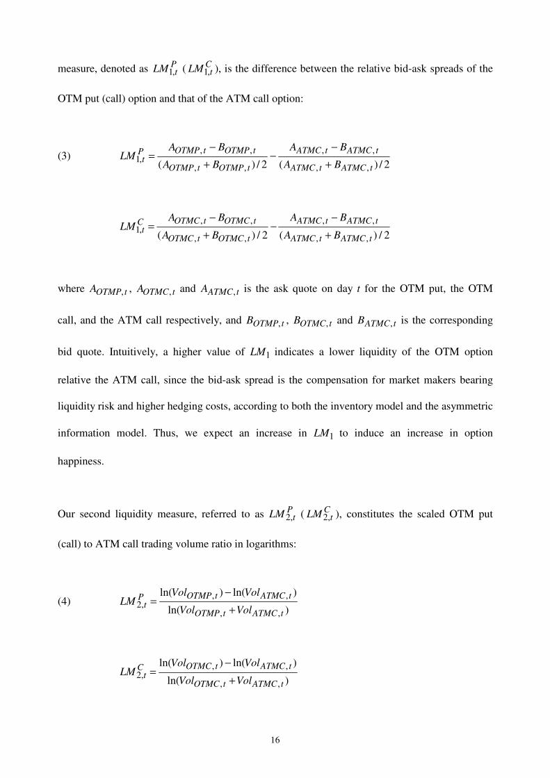
measure, denoted as PtLM ,1 ( C

tLM ,1 ), is the difference between the relative bid-ask spreads of the

OTM put (call) option and that of the ATM call option:

(3) 2/)(2/)( ,,

,,

,,

,,,1

tATMCtATMC

tATMCtATMC

tOTMPtOTMP

tOTMPtOTMPPt

BA

BA

BA

BALM

+

−−

+

−=

2/)(2/)( ,,

,,

,,

,,,1

tATMCtATMC

tATMCtATMC

tOTMCtOTMC

tOTMCtOTMCCt

BA

BA

BA

BALM

+

−−

+

−=

where tOTMPA , , tOTMCA , and tATMCA , is the ask quote on day t for the OTM put, the OTM

call, and the ATM call respectively, and tOTMPB , , tOTMCB , and tATMCB , is the corresponding

bid quote. Intuitively, a higher value of 1LM indicates a lower liquidity of the OTM option

relative the ATM call, since the bid-ask spread is the compensation for market makers bearing

liquidity risk and higher hedging costs, according to both the inventory model and the asymmetric

information model. Thus, we expect an increase in 1LM to induce an increase in option

happiness.

Our second liquidity measure, referred to as PtLM ,2 ( C

tLM ,2 ), constitutes the scaled OTM put

(call) to ATM call trading volume ratio in logarithms:

(4) )ln(

)ln()ln(

,,

,,,2

tATMCtOTMP

tATMCtOTMPPt

VolVol

VolVolLM

+

−=

)ln(

)ln()ln(

,,

,,,2

tATMCtOTMC

tATMCtOTMCCt

VolVol

VolVolLM

+

−=

17

where tOTMPVol , , tOTMCVol , and tATMCVol , is the trading volume on day t (number of traded

contracts) for the OTM put, the OTM call, and the ATM call respectively.

The liquidity measure 2LM can be seen as a more well-defined version of the trading volume

ratio in Dennis and Mayhew (2002), which they use as a proxy for trading pressure. Bollen and

Whaley (2004) claim that trading volume might not be an accurate proxy for net buying pressure.

Daily trading volume is simply the result of buy- and sell-order matching throughout the trading

day, and contains no information of whether the trades are buyer- or seller-initiated. Thus, we

argue that 2LM should be used rather as a measure of relative liquidity than a net buying pressure

proxy. However, higher trading volume may imply either higher liquidity or lower liquidity of

each option contract. First, if normal liquidity traders are considered as the main driving force

behind the trading activity, then a larger trading volume is interpreted as an improvement in

liquidity of the option contract in question. With more active trading in the option contract, the

probability of ending up with a large net position is lower, and the market makers are less

exposed to liquidity risk. Hence, an increase in 2LM is in this case an indication of a higher

liquidity of the OTM put or OTM call relative to the ATM call, and a decrease in option

happiness is expected. Second, if informed traders are thought to be the main source behind the

trading activity, then a larger trading volume is interpreted as a lower liquidity of the option

contract. Therefore, an increase in 2LM would be an indication of a lower liquidity of the OTM

put or OTM call relative to the ATM call, and an increase in option happiness is expected. We

argue that the first case is the most reasonable situation for an index option market, since the bulk

of trading is unlikely to be generated by informed traders.

The third liquidity measure, denoted as PtLM ,3 ( C

tLM ,3 ), originates from Grossman and Miller

(1988), the illiquidity measure from Amihud (2002), and the liquidity ratio measure in earlier

18

studies (see Dubofsky and Groth, 1984; Cooper et al., 1985; and Martin, 1975). With reference to

the stock market, Grossman and Miller (1988) suggest that inter-temporal price movements might

provide a more accurate reflection of the “cost” of stock illiquidity. Amihud (2002) uses the daily

ratio of absolute stock return to its dollar volume (averaged over some period) to measure

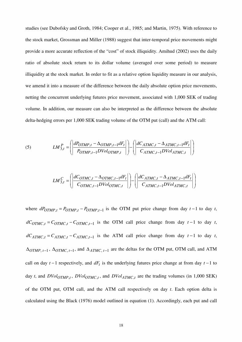
illiquidity at the stock market. In order to fit as a relative option liquidity measure in our analysis,

we amend it into a measure of the difference between the daily absolute option price movements,

netting the concurrent underlying futures price movement, associated with 1,000 SEK of trading

volume. In addition, our measure can also be interpreted as the difference between the absolute

delta-hedging errors per 1,000 SEK trading volume of the OTM put (call) and the ATM call:

(5)

∆−−

∆−=

−

−

−

−

tATMCtATMC

ttATMCtATMC

tOTMPtOTMP

ttOTMPtOTMPPt

DVolC

dFdC

DVolP

dFdPLM

,1,

1,,

,1,

1,,,3

∆−−

∆−=

−

−

−

−

tATMCtATMC

ttATMCtATMC

tOTMCtOTMC

ttOTMCtOTMCCt

DVolC

dFdC

DVolC

dFdCLM

,1,

1,,

,1,

1,,,3

where 1,,, −−= tOTMPtOTMPtOTMP PPdP is the OTM put price change from day 1−t to day t,

1,,, −−= tOTMCtOTMCtOTMC CCdC is the OTM call price change from day 1−t to day t,

1,,, −−= tATMCtATMCtATMC CCdC is the ATM call price change from day 1−t to day t,

1, −∆ tOTMP , 1, −∆ tOTMC , and 1, −∆ tATMC are the deltas for the OTM put, OTM call, and ATM

call on day 1−t respectively, and tdF is the underlying futures price change at from day 1−t to

day t, and tOTMPDVol , , tOTMCDVol , , and tATMCDVol , are the trading volumes (in 1,000 SEK)

of the OTM put, OTM call, and the ATM call respectively on day t. Each option delta is

calculated using the Black (1976) model outlined in equation (1). Accordingly, each put and call

19

option delta equals )( 1dN − and )( 1dN respectively. In each delta calculation, we use the realized

index return volatility over the most recent sixty trading days as a proxy for the volatility rate tσ .

An increase in PLM3 ( C

LM3 ) can be interpreted as an increase in the daily OTM put (call) option

price response associated with a trading volume of one thousand SEK, relative to the daily ATM

call option price response, which implies a lower relative liquidity of the OTM put (call) relative

the ATM call. Moreover, if market makers face larger delta-hedging errors in the OTM put (call)

rather than the ATM call, they would charge a relative higher option price for the OTM put (call),

resulting in a higher IV of the OTM put (call) relative to the ATM call (generating a positive

option happiness). Hence, we expect a positive relationship between 3LM and option happiness.

More specifically, the larger the difference in trading volume adjusted delta-hedging errors

between the OTM put (call) and the ATM call, the larger put (call) option happiness will be.

3.2 Regression models

To investigate the impacts of relative option liquidity on option happiness, we use a dynamic

regression model specification, where the daily development of option happiness depends on the

contemporaneous measures of relative option liquidity. The dynamic framework is motivated by

previous studies finding evidence of return volatility clustering and persistence of volatility.18

Thus, a persistence property may be anticipated in option happiness as well, and consequently, we

include the lagged option happiness and lagged relative liquidity measures as control variables in

the regression framework. In addition, we include time to maturity as a control variable since

many studies report that the volatility smirk has a time to maturity effect, which is often referred

to as the IV term structure (see e.g. Das and Sundaram, 1999; and Duque and Teixeira, 2003).

18

See e.g. Bollerslev et al. (1992), and Poterba and Summers (1986).

20

Our basic regression model is specified as:

(6) 1,,1,,,1,,,,,1, ++++ ++++=− tjitjii

tjjii

tjjijitijiti uTimeLMLMOHOH δγβαφ

where the index i = P and C represents option happiness for the OTM put and OTM call

respectively as in equation (2), the index j = 1, 2, and 3, represents the three different relative

liquidity measures from equation (3) through (5), tTime is the option time to maturity on day t,

ji,φ , ji,α , ji,β , ji,γ , ji,δ are coefficients in each regression equation of option happiness i on

relative liquidity measure j, and tjiu ,, is a corresponding regression residual term on day t.

The regression analysis of the dynamics of option happiness and relative liquidity according to

equation (6) will follow the same individual option contracts from day t to the following day

1+t . Thus, for each combination of option happiness i and relative liquidity measure j = 1 and 2

(the relative bid-ask spread and relative trading volume measures), we find the OTM put or call

and corresponding ATM call option on day t, obtain the measures tiOH , and itjLM , , and follow

the same option contracts to the following day 1+t to obtain 1, +tiOH and itjLM 1, + . The other

relative liquidity measure j = 3 (the inter-temporal price impact measure) already involve the

calculation of option hedging errors from day t to day 1+t according to equation (5). Therefore,

the regression equation (6) will not include the variable itjLM , for j = 3.

Our main purpose is to investigate whether relative option liquidity across moneyness helps

explain the time variation in option happiness. The regression model in equation (6) is designed

to test the effect of each different relative liquidity measure on option happiness. Formally, a test

21

of the statement that liquidity measure j has no contemporaneous impact on option happiness

measure i, boils down to test the following null hypothesis:

(7) 1H : 0, =jiβ

against the alternative that 0, ≠jiβ .

In addition, to examine whether the each of the first two relative liquidity measures explored in

this study, j = 1 and 2, can help improve the prediction of option happiness, each lagged relative

liquidity measure is included in the regression model (6). Consequently, we test the hypothesis

that the relative liquidity measure j has no predictive power for the option happiness measure i:

(8) 2H : 0, =jiγ

against the alternative that 0, ≠jiγ .

Our different liquidity measures may capture different dimensions of relative option liquidity. In

order to jointly investigate the relative liquidity effects on option happiness, we extend the

regression model in equation (6) to:

(9) 1,1

2

1

,,

3

1

1,,,1, ++==

++ ′+′+′+′+′=′− ∑∑ titi

j

itjji

j

itjjiitiiti uTimeLMLMOHOH δγβαφ

where iφ ′ , iα ′ , ji,β ′ , ji,γ ′ , iδ ′ are regression coefficients, and tiu ,′ is a residual term. Within the

extended regression in equation (9) it is possible to perform individual tests of whether each

relative liquidity measure affects option happiness contemporaneously by testing the hypothesis

22

according to equation (7) for each ji,β ′ coefficient, and individual tests of whether each of the

two relative liquidity measures itLM ,1 and i

tLM ,2 has predictive power for option happiness by

testing the corresponding hypothesis in equation (8) for each ji,γ ′ coefficient. Moreover, we

perform the joint test of the null hypothesis that none of the relative liquidity measures has a

contemporaneous effect on option happiness:

(10) 3H : 0, =′ jiβ for all j = 1, 2, 3

against the alternative that at least one 0, ≠′ jiβ . Similarly, a joint test of the null hypothesis that

none of the first two relative liquidity measures has predictive power for option happiness is:

(11) 4H : 0, =′ jiγ for all j = 1, 2

against the alternative that at least one 0, ≠′ jiγ .

3.3 Data

The data set consists of daily closing prices for OMXS 30 index options and futures contracts

from January 2, 2004 to December 30, 2005, obtained from NASDAQ-OMX, including

information of futures and options quotes (closing bid-ask quotes, last transaction prices, daily

high and low transaction prices), and trading volume (number of traded contracts) for each option

and futures contract. Additional data, also obtained from NASDAQ-OMX, include daily OMXS

30 index values for the sample period. The one-month Stockholm Interbank Rate (STIBOR) is

23

used as a proxy for the risk-free rate of interest, and is downloaded from the Riksbank’s

website.19

The data used in describing the properties of volatility smirk pattern satisfy several screening

requirements. We include all options with time to maturity between one week to six weeks that

have non-zero trading volume and non-zero bid-ask quotes. In addition, the very deep ITM and

the very deep OTM options are discarded, since they are seldom traded. Specifically, deep ITM

calls (puts) with option delta larger than 0.98 (less than -0.98) and deep OTM calls (puts) with

delta less than 0.02 (larger than -0.02) are dropped. In all, we retain 7,336 option contract

observations after the data screening.

The data used in the dynamic regression analysis consists of daily observations on the nearest-to-

expiration options and futures with at least one week left to maturity. Following most studies in

this field, on the seventh day before expiration, we switch to the next corresponding contract in

the maturity cycle.20

Since the dynamic analysis, and calculation of option happiness and relative

liquidity measures, follows the same option contracts from one day until the following trading

day, we require the options to be traded on two consecutive trading days. The number of daily

observations equals 506 in the dynamic regression setup.

4. Empirical results

4.1 The properties of the volatility smirk in OMXS30 index options

19

www.riksbank.se 20

The reasons are: (1) the time value of very short-lived options relative to their bid-ask spreads is small, and (2) the

set of traded strike prices shrinks as expiration approaches (Ederington and Guan, 2002).

24

In order to illustrate the volatility smirk pattern for the OMXS30 index options, we classify the

options into five moneyness categories. Following Bollen and Whaley (2004), we use the option

delta as the classification criterion as shown in Table 1.21

For each moneyness category, we

compute the average IV for calls and puts separately over the entire sample period. The results are

reported in Table 1, where Panel A (B) contains the results for the calls (puts). In total, 7,336

observations fall into one of the five moneyness groups. For calls and puts alike, the category 3

(ATM) options comprise about one third of the total observations while category 1 and category 5

options together only represent around 10% of the total observations. In particular, we have only

40 deep ITM put observations. The call options show a strictly decreasing IV pattern across the

moneyness groups. Note that the average IV of the deep ITM calls is 17.18%, about 24% higher

than the average IV of deep OTM calls of 13.81%. Moreover, the corresponding IV pattern for

put options is decreasing between categories 1 and 4, but increases in category 5 (deep ITM puts).

For both calls and puts, the average IV, relative the concurrent ATM call IV, is decreasing over

the option categories 1 through 4, and increasing between categories 4 and 5. As can be seen in

Figure 1, where the average relative IV is plotted over the five option categories, both OMXS30

index calls and puts show clear evidence of an implied volatility smirk. In addition, using the

figures in Table 1, the average put option happiness can be inferred on an option category basis

from the percentage difference between the average IV for OTM put options (0.1647) and the

average IV for ATM call options (0.1540). The corresponding average call option happiness

measure can be calculated as the percentage difference between the average OTM call IV

21

As explained in Bollen and Whaley (2004), all of the delta pairings for the calls and puts are based on put-call

parity. For example, a put with a delta of -0.125 should have the same implied volatility as a call with a delta equal to

0.875. The reason for grouping the options by deltas instead of the conventional simple moneyness, e.g. the strike to

current futures price ratio, is that the former takes into account the fact that the likelihood of the option being

exercised not only depends on moneyness but also on the time left to maturity and the volatility rate.

25

(0.1434) and the average ATM call IV (0.1540). Thus, the average put (call) option happiness is

about 7% (-7%) over the sample period.22

Table 1 also reports the average daily trading volume and relative bid-ask spread for each call and

put option category. The average trading volume figures clearly indicate that OTM and ATM

options are more actively traded than the ITM options. In addition, for both calls and puts, the

average relative bid-ask spread shows a U-shaped pattern over the moneyness categories, with the

lowest level for ITM options. With the subsequent analysis of option happiness in mind, we note

that the OTM calls and OTM puts on average have wider relative bid-ask spreads than the ATM

calls. Though, all three option types are on average approximately equally actively traded.

4.2 Summary statistics for option happiness and IVs

We next focus on the options used in our dynamic regression analysis. Thus, on a daily basis, we

follow an ATM call, an OTM put and an OTM call to the subsequent trading day, and calculate

each call and put option happiness measure according to equation (2). Table 2 contains summary

statistics for the option IVs and option happiness measures. As can be seen in Table 2, the

average OTM put IV equals 0.1659, which is about 10% higher than the average ATM call IV

(0.1505), which in turn is about 4% higher than the average OTM call IV (0.1447).23

In addition,

put option happiness is on average positive, with an estimated mean equal to 0.1115, whereas call

option happiness is on average negative, with a corresponding estimated mean of -0.0382.24

22

Note however that these averages include all options in each moneyness category, irrespective of maturity. In our

following analysis, we use the more distinct definition of option happiness on a specific day, in equation (2), using an

OTM put (call) and an ATM call with a fixed strike price difference, and the same maturity. 23

A formal t-test of the hypothesis of equality between the average OTM put (call) IV and the average ATM call IV

results in a p-value of 0.0000 (0.0000), i.e. a rejection of the hypothesis at any reasonable significance level. 24

A formal t-test of the hypothesis that the average put (call) option happiness equals zero results in a p-value of

0.0000 (0.0000), i.e. a rejection of the hypothesis at any reasonable significance level.

26

These figures lend support to our observation of a significant smirk pattern in the OMXS30 index

options.

Table 2 also presents the results from a unit root test for stationarity of each variable. An

augmented Dickey-Fuller test (see Fuller, 1996) is used to test each individual null hypothesis

that the time series has a unit root. Using the p-values from MacKinnon (1996), it is possible to

reject each null hypothesis of a unit root for put and call option happiness at any reasonable

significance level. However, each corresponding null hypothesis for the IV variables cannot be

rejected at the 5% significance level. Hence, we consider the option happiness variables to be

stationary, which enable us to use these time series directly in the dynamic regression analysis.

Figure 2 illustrates the time series properties of call and put option happiness over the sample

period. We also show the corresponding development of the ATM call IV. A prominent

characteristic of this figure is that option happiness evolves dramatically over time, and put option

happiness more dramatically than call option happiness, while the ATM call IV behaves relatively

smoothly. In addition, put option happiness is with few exceptions always above zero, while call

option happiness is mostly below zero.

4.3 Summary statistics for the relative liquidity measures

Table 3 provides summary statistics for the relative bid-ask spread, and trading volume for the

OMXS30 index options used in the dynamic regression analysis. In general, the ATM options are

regarded as the most liquid options. This is further confirmed in our data with an average relative

bid-ask spread of 0.0756 and an average trading volume of 2,408, compared with an average

27

relative bid-ask spread for the OTM put (call) of 0.1170 (0.1326) and an average trading volume

of 1,955 (2,150).25

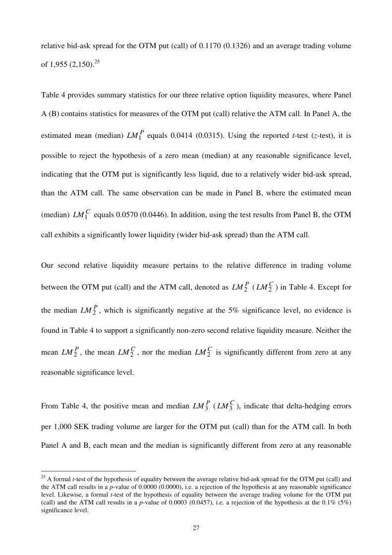
Table 4 provides summary statistics for our three relative option liquidity measures, where Panel

A (B) contains statistics for measures of the OTM put (call) relative the ATM call. In Panel A, the

estimated mean (median) PLM1 equals 0.0414 (0.0315). Using the reported t-test (z-test), it is

possible to reject the hypothesis of a zero mean (median) at any reasonable significance level,

indicating that the OTM put is significantly less liquid, due to a relatively wider bid-ask spread,

than the ATM call. The same observation can be made in Panel B, where the estimated mean

(median) CLM1 equals 0.0570 (0.0446). In addition, using the test results from Panel B, the OTM

call exhibits a significantly lower liquidity (wider bid-ask spread) than the ATM call.

Our second relative liquidity measure pertains to the relative difference in trading volume

between the OTM put (call) and the ATM call, denoted as PLM 2 ( CLM 2 ) in Table 4. Except for

the median PLM 2 , which is significantly negative at the 5% significance level, no evidence is

found in Table 4 to support a significantly non-zero second relative liquidity measure. Neither the

mean PLM 2 , the mean CLM 2 , nor the median CLM 2 is significantly different from zero at any

reasonable significance level.

From Table 4, the positive mean and median PLM 3 ( C

LM3 ), indicate that delta-hedging errors

per 1,000 SEK trading volume are larger for the OTM put (call) than for the ATM call. In both

Panel A and B, each mean and the median is significantly different from zero at any reasonable

25

A formal t-test of the hypothesis of equality between the average relative bid-ask spread for the OTM put (call) and

the ATM call results in a p-value of 0.0000 (0.0000), i.e. a rejection of the hypothesis at any reasonable significance

level. Likewise, a formal t-test of the hypothesis of equality between the average trading volume for the OTM put

(call) and the ATM call results in a p-value of 0.0003 (0.0457), i.e. a rejection of the hypothesis at the 0.1% (5%)

significance level.

28

significance level. In addition, each relative liquidity measure is regarded as a stationary time

series since each unit root test results in a rejection of the null hypothesis of a unit root at a very

low significance level. Hence, all relative liquidity measures can be used in the subsequent

dynamic regression analysis without further transformations.

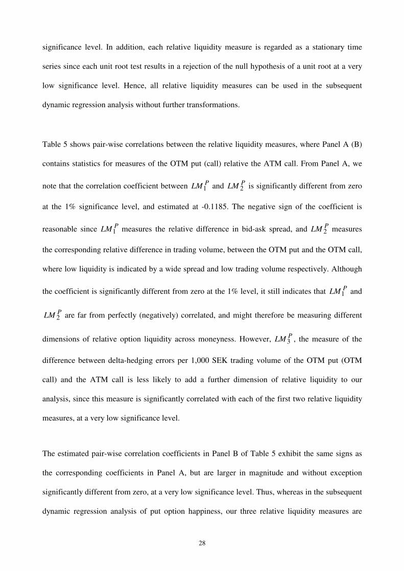
Table 5 shows pair-wise correlations between the relative liquidity measures, where Panel A (B)

contains statistics for measures of the OTM put (call) relative the ATM call. From Panel A, we

note that the correlation coefficient between PLM1 and PLM 2 is significantly different from zero

at the 1% significance level, and estimated at -0.1185. The negative sign of the coefficient is

reasonable since PLM1 measures the relative difference in bid-ask spread, and PLM 2 measures

the corresponding relative difference in trading volume, between the OTM put and the OTM call,

where low liquidity is indicated by a wide spread and low trading volume respectively. Although

the coefficient is significantly different from zero at the 1% level, it still indicates that PLM1 and

PLM 2 are far from perfectly (negatively) correlated, and might therefore be measuring different

dimensions of relative option liquidity across moneyness. However, PLM3 , the measure of the

difference between delta-hedging errors per 1,000 SEK trading volume of the OTM put (OTM

call) and the ATM call is less likely to add a further dimension of relative liquidity to our

analysis, since this measure is significantly correlated with each of the first two relative liquidity

measures, at a very low significance level.

The estimated pair-wise correlation coefficients in Panel B of Table 5 exhibit the same signs as

the corresponding coefficients in Panel A, but are larger in magnitude and without exception

significantly different from zero, at a very low significance level. Thus, whereas in the subsequent

dynamic regression analysis of put option happiness, our three relative liquidity measures are

29

likely to represent different dimensions of relative liquidity, this is less likely in the corresponding

analysis of call option happiness. Hence, the extended regression model in equation (9) is

potentially more appropriate for put option happiness than call option happiness, where in the

former specification, we are more likely to be able to discern between the effects of the different

relative liquidity measures, and are less likely to encounter multicollinearity problems.

4.4 Regression results

We start our dynamic analysis of option happiness by estimating the basic regression models

according to equation (6). Each regression model is estimated using non-linear least squares,

adding autoregressive residual terms in a stepwise fashion to take residual autocorrelation into

account. In each stepwise analysis, we add autoregressive residual terms until the Breusch-

Godfrey serial correlation LM test shows no autocorrelation (up to 10 lags) left in the residuals.

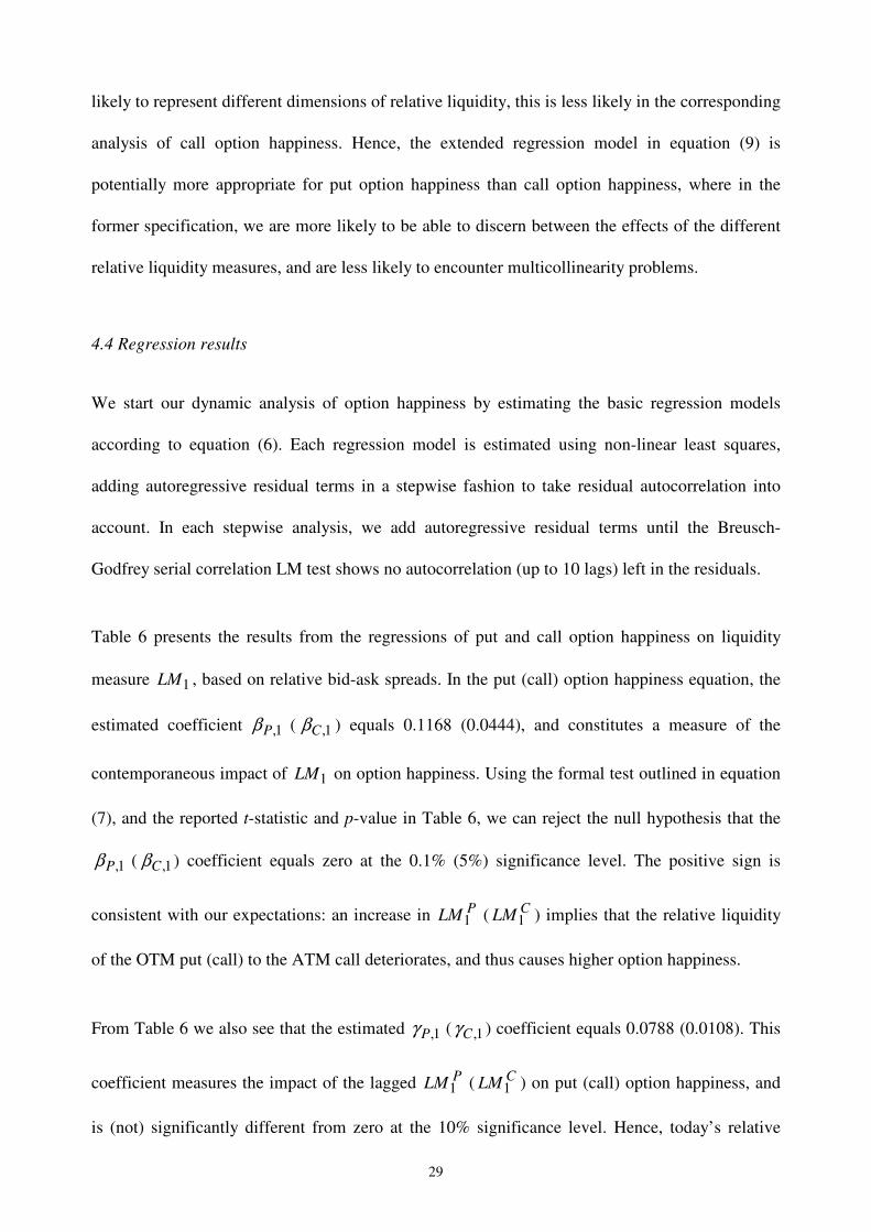
Table 6 presents the results from the regressions of put and call option happiness on liquidity

measure 1LM , based on relative bid-ask spreads. In the put (call) option happiness equation, the

estimated coefficient 1,Pβ ( 1,Cβ ) equals 0.1168 (0.0444), and constitutes a measure of the

contemporaneous impact of 1LM on option happiness. Using the formal test outlined in equation

(7), and the reported t-statistic and p-value in Table 6, we can reject the null hypothesis that the

1,Pβ ( 1,Cβ ) coefficient equals zero at the 0.1% (5%) significance level. The positive sign is

consistent with our expectations: an increase in PLM1 ( CLM1 ) implies that the relative liquidity

of the OTM put (call) to the ATM call deteriorates, and thus causes higher option happiness.

From Table 6 we also see that the estimated 1,Pγ ( 1,Cγ ) coefficient equals 0.0788 (0.0108). This

coefficient measures the impact of the lagged PLM1 ( CLM1 ) on put (call) option happiness, and

is (not) significantly different from zero at the 10% significance level. Hence, today’s relative

30

option liquidity in terms of observed relative bid-ask spreads contains some information about

future put option happiness. However, in the equation for call option happiness, including lagged

CLM1 does not significantly help the prediction of option happiness.

The estimation results of the dynamic regression equations presented in Table 6 show clear

evidence of persistence in both put and call option happiness. The coefficient 1,Pφ ( 1,Cφ ) of the

lagged put (call) option happiness is significantly positive at a very low significance level. Thus,

in terms of prediction, the current level of option happiness appears to contain significant

information of the future level of option happiness. The positive relationship between option

happiness and lagged option happiness also corroborates the findings in previous research (See

e.g. Bollerslev et al., 1992, Poterba and Summers, 1986), that volatility tends to be highly

persistent in short time intervals. Moreover, another sign of persistence in each equation is the

large number of residual lags required for passing the Breusch-Godfrey LM test.

The results in Table 6 reveal a significantly negative relationship between put option happiness

and option time to maturity, at the 1% significance level, with an estimated 1,Pδ coefficient equal

to -0.3063. The corresponding 1,Cδ coefficient, measuring the relationship between call option

happiness and maturity, is not significantly different from zero at any significance level. The

negative relationship between option time to maturity and the steepness of the volatility smirk,

represented by put option happiness, is consistent with the findings in previous studies (see e.g.

Das and Sundaram, 1999; Duque and Teixeira, 2003), which indicates that the OMXS30 index

options market displays a more pronounced smirk when the options approach the maturity date,

i.e. the options are dying smiling.

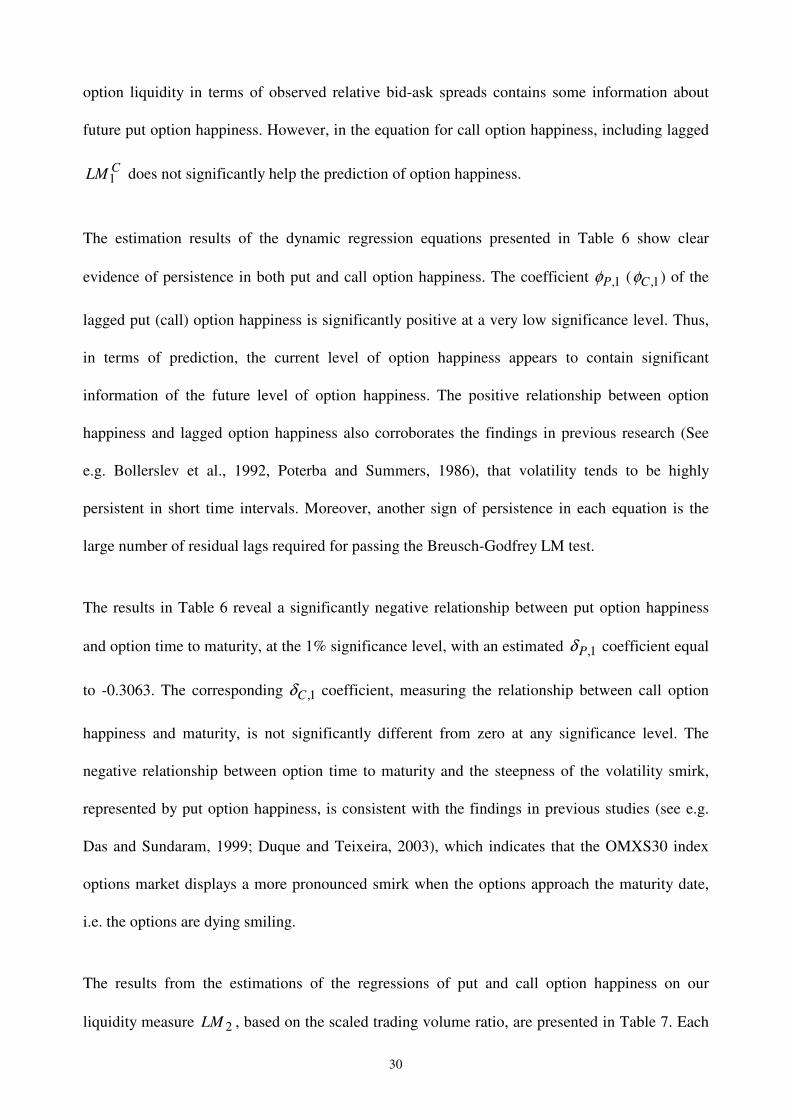
The results from the estimations of the regressions of put and call option happiness on our

liquidity measure 2LM , based on the scaled trading volume ratio, are presented in Table 7. Each

31

estimated coefficient 2,Pβ and 2,Cβ is negative. Moreover, the coefficient 2,Cβ in the call

option happiness regression equation is significantly negative at the 0.1% significance level,

whereas the corresponding coefficient 2,Pβ in the put option happiness equation is not

significantly different from zero at any reasonable significance level. The significantly negative

sign of the coefficient for CLM 2 in the call option happiness equation is consistent with the idea

that market makers generally interpret the relatively high trading volume in index options as

trading activity driven by normal liquidity traders rather than informed traders. Thus, the higher

trading activity in the OTM call relative to the ATM call would reduce the risk of holding large

net positions in the OTM call compared to the ATM call. In this case, an increase in CLM 2

implies that the relative liquidity of the OTM call to the ATM call is improved and hence, induces

a lower call option happiness.

In Table 7, for each put and call option happiness equation, the coefficient of lagged 2LM is not

significantly different from zero at any reasonable significance level, which implies that the

current relative option trading activity holds little information content about future option

happiness. The remaining coefficients in each equation in Table 7 resemble the corresponding

ones from Table 6, both with respect to the coefficient levels and their significance.

The third liquidity measure 3LM is based on the inter-temporal option price movement

associated with 1,000 SEK of trading volume, which also can be interpreted as the relative delta-

hedging error per 1,000 SEK of trading volume of the OTM put (call) to the ATM call. Table 8

contains the results from the regressions of put and call option happiness on 3LM . As can be

seen in Table 8, the 3,Pβ ( 3,Cβ ) coefficient is positive and (not) significantly different from zero

at any reasonable significance level. The positive sign of in particular the coefficient in the put

32

option happiness equation is in accordance with our expectations. An increase in PLM3 is an

indication of lower relative option liquidity in the OTM put to the ATM call, and would

according to our results lead to a significant increase in option happiness. Market makers would

charge a higher price for the OTM put option with larger delta-hedging errors per 1,000 SEK of

trading volume, which consequently implies a higher IV of the OTM put option relative to the

ATM call.

In our effort to investigate relative liquidity effects on option happiness, we employ the

multivariable dynamic setup according to equation (9), including all the relative liquidity

measures and control variables, and recognizing that the different measures may capture different

dimensions of liquidity. The regression results are displayed in Table 9. The joint test of the null

hypothesis that not a single relative liquidity measure has a contemporaneous effect on put (call)

option happiness, as formalized in equation (10), is performed using a Wald-type chi-square test.

Accordingly, in the put (call) option happiness equation, the null hypothesis is rejected at a very

low (the 1%) significance level. However, each corresponding null hypothesis from equation

(11), that none of the first two relative liquidity measures has predictive power for option

happiness, cannot be rejected at any reasonable significance level. Hence, for both put and call

option happiness, the contemporaneous effects from the relative liquidity measures persist in the

joint dynamic framework, whereas the corresponding lagged effects do not.

Having a closer look at the individual coefficients for the relative liquidity measures in Table 9,

we observe that the 1,Pβ ′ ( 3,Pβ ′ ) coefficient in the put option happiness equation is significantly

different from zero at the 5% (0.1%) significance level, whereas the 2,Pβ ′ coefficient is not

significantly different from zero at any reasonable significance level. These results confirm the

results from the corresponding basic regression analyses, presented in Table 6 through 8.

33

However, when comparing the estimated levels for the significant 1,Pβ ′ and 3,Pβ ′ coefficients in

the joint regression in Table 9, 0.0876 and 0.1153 respectively, with the corresponding estimated

basic regression coefficients 0.1168 and 0.1457, from Table 6 through 8, we notice that the joint

regression framework produces somewhat lower coefficient estimates (and higher significance

levels). Nevertheless, the fact that put option happiness is still significantly related to

contemporaneous relative liquidity, measured by relative bid-ask spreads and volume-adjusted

relative delta hedging errors, confirms our notion that the implied volatility smirk is generated by

relative option liquidity. Moreover, since 1LM and 3LM are associated with significant

coefficients in both the separate models for put option happiness according to equations (6)

through (8), and the joint model in equation (9), our liquidity measures are likely to capture

different dimensions of relative option liquidity.

In Table 9, for the call option happiness equation, we observe that the 2,Cβ ′ coefficient is

significantly different from zero at the 5% significance level, whereas the coefficients 1,Cβ ′ and

1,Cβ ′ are not significantly different from zero at any reasonable significance level. Thus, call

option happiness is still significantly related to 2LM , the relative trading volume difference

between the OTM call and the ATM call option. However, whereas 1LM , the corresponding

relative difference between the options’ bid-ask spreads, is associated with a significant

coefficient in the basic regression setup in Table 6, it is not a significant determinant of call

option happiness in the joint dynamic regression model. Therefore, it is fair to conclude that the

effect from 2LM ( 1LM ) on call option happiness is (not) robust against including all relative

liquidity measures into the joint dynamic specification. Moreover, the estimated 2,Cβ ′ coefficient

(-0.0226) is only slightly lower (in absolute terms) than the corresponding estimate of 2,Cβ (-

0.0280) in the basic regression model in Table 7.

34

In all, daily option happiness (the steepness of the volatility smirk) is significantly dependent on

the concurrent relative liquidity between option series with different moneyness. In particular, a

larger liquidity difference between the OTM put option and the concurrent ATM call option leads

to a larger option happiness. We argue that our liquidity measures capture different dimensions of

option liquidity. Accordingly, put option happiness is significantly related to the difference

between the relative bid-ask spreads, and the trading volume-adjusted delta-hedging errors, of the

OTM put and the ATM call option, whereas call option happiness only is significantly affected by

the difference in trading volume between the OTM call and the ATM call. Interestingly, the slope

of the implied volatility function, as displayed in Figure 1, is affected by different dimensions of

relative option liquidity for category 2 options (to the left in Figure 1) and category 4 options (to

the right) respectively.

5. Concluding remarks

We investigate the dynamic relationship between relative option liquidity and option happiness

(the steepness of the implied volatility smirk). The idea behind the alleged relationship between

option happiness and liquidity rests on the notion that in reality, unlike in the pseudo world of

theoretical option valuation, options’ markets exhibit constraints to arbitrage and perfect hedging.

In a market where options with different moneyness are traded at different degrees of liquidity,

market makers are likely to quote option prices including a liquidity premium. Thus, options with

relative low (high) liquidity are expected to be relatively higher (lower) priced, which of course

implies a relatively higher (lower) volatility for options with low (high) liquidity.

We use two option happiness measures in order to cover as large part of the volatility smirk, and

as wide range of option moneyness, as possible. First, we measure put option happiness as the

relative difference between the implied volatility of an out-of-the-money put and the implied

35

volatility of an at-the-money call, with identical maturity. Second, our corresponding measure of

call option happiness is obtained as the relative difference between the implied volatility of an

out-of-the-money call and the implied volatility of an at-the-money call.

Liquidity is notoriously difficult to measure; almost like the hydra of financial markets. Once the

researcher believes he/she has found the correct measure of liquidity, using e.g. the bid-ask spread

as a proxy for the market width, out pops three other dimensions, depth, immediacy and

resiliency, calling for the use of multiple liquidity proxies. Hence, taking the multi-dimensionality

of liquidity into account, we include three different relative option liquidity measures in our

dynamic analysis of option happiness; relative bid-ask spreads, relative trading volume, and

volume adjusted relative delta hedging errors (an option version of Amihud’s, 2002, illiquidity

measure in relative sense).

Our purpose, and contribution to previous work, is at least threefold. First, we document the

volatility smirk for the Swedish index options market, which no one has done before us. Second,

we introduce the concept of option happiness, which allows us to investigate the dynamic

properties of a large part of the implied volatility smirk. Third, we analyze the dynamic

relationship between option happiness and relative option liquidity. For this purpose, we develop

comprehensive measures of option liquidity, focusing on the relative liquidity between option

series with different moneyness. Unlike previous studies, e.g. Bollen and Whaley (2004) and

Gârleanu et al. (2007), our analysis is not contaminated by potential biases from averaging

implied volatilities and relative liquidity over several option contracts.

Our findings show a significant implied volatility smirk and a time-to-maturity effect in the

Swedish index options market. We also find significant differences in liquidity between options

with different moneyness. These effects appear to be persistent over the entire sample period. Our

36

main results show that daily option happiness is significantly dependent on our relative liquidity

measures, where a large difference in liquidity between an out-of-the-money option and a

corresponding at-the-money call option induces large option happiness. This relationship is

stronger for our put option happiness measure than for the call option happiness measure.

Accordingly, put option happiness is significantly related to the relative difference in bid-ask

spreads and the relative volume-adjusted delta-hedging errors, whereas call option happiness is

significantly related to the relative difference in trading volume between the option pair. In

addition, we find that higher put option happiness is accompanied with less time to maturity of

the options. Thus, the Swedish index put options are showing a tendency for “dying smiling”,

consistent with previous studies.

Bibliography

Acharya, V., and L. Pedersen, 2005, Asset pricing with liquidity risk, Journal of Financial

Economics 77, 375-410.

Amihud, Y., 2002, Illiquidity and stock returns: cross-section and time-series effects, Journal of

Financial Markets 5, 31-56.

Amihud, Y., and H. Mendelson, 1986, Asset pricing and the bid-ask spread, Journal of Financial

Economics 17, 223-249.

Amin, K., and V. Ng, 1993, Option valuation with systematic stochastic volatility, Journal of

Finance 48, 881-910.

37

Bakshi, G., Cao, C., and Z. Chen, 1997, Empirical performance of alternative option pricing

models, Journal of Finance 52, 2003-2049.

Bakshi, G., and Z. Chen, 1997, Equilibrium valuation of foreign exchange claims, Journal of

Finance 52, 799-826.

Bates, D., 2000, Post-’87 crash fears in the S&P 500 futures options market, Journal of

Econometrics 94, 181-238.

Bates, D., 2003, Empirical option pricing: A retrospection, Journal of Econometrics 116, 387-

404.

Bates, D., 2006, Maximum likelihood estimation of latent affine processes, Review of Financial

Studies 19, 909-965.

Black, F., 1976, The pricing of commodity contracts, Journal of Financial Economics 3, 167-179.

Black, F., and M. Scholes, 1973, The pricing of options and corporate liabilities, Journal of

Political Economy 81, 637-659.

Bollen, N., and R. Whaley, 2004, Does net buying pressure affect the shape of implied volatility

functions? Journal of Finance 59, 711-753.

Bollerslev, T., Chou, R., and K. Kroner, 1992, ARCH Modeling in Finance: A review of the

theory and empirical evidence, Journal of Econometrics 52, 5-59.

38

Cao, M. and J. Wei, 2008, Option market liquidity: Commonality and other characteristics.

Forthcoming in Journal of Financial Markets.

Çetin, U., Jarrow R., Protter P., and M. Warachka, 2006, Pricing options in an extended Black

Scholes economy with illiquidity: Theory and empirical evidence, Review of Financial Studies

19, 493-529.

Chou, R., Chung, S., Hsiao, Y., and Y. Wang, 2009, The impacts of liquidity risk on option

prices. Available at SSRN: http://ssrn.com/abstract=1467403

Cooper, K., Groth, J., and W. Avera, 1985, Liquidity, exchange listing, and common stock

performance, Journal of Economics and Business 37, 19-33.

Das, S., and R. Sundaram, 1999, Of smiles and smirks: A term-structure perspective, Journal of

Financial and Quantitative Analysis 34, 211-239.

Dennis, P., and S. Mayhew, 2002, Risk-neutral skewness: Evidence from stock options, Journal

of Financial and Quantitative Analysis 37, 471-493.

Demsetz, H., 1968, The cost of transacting, Quarterly Journal of Economics 82, 33-53.

Deuskar, P., Gupta, A., and M. Subrahmanyam, 2008, The economic determinants of interest rate

option smiles, Journal of Banking and Finance 32, 714-728.

Dubofsky, F., and J. Groth, 1984, Exchange listing and stock liquidity, Journal of Financial

Research 7, 291-302.

39

Dumas, B., Fleming, J., and R. Whaley, 1998, Implied volatility functions: Empirical tests,

Journal of Finance 53, 2059-2106.

Dupire, B., 1994, Pricing with a smile, Risk 7, 18-20.

Duque, J., and L. Teixeira, 2003, Maturity and volatility effects on UK smiles. Or dying smiling?

Portuguese Economics Journal 2, 173-193.

Easley, D. and M. O’Hara, 1987, Price, trade size, and information in securities markets, Journal

of Financial Economics 19, 69-90.

Easley, D., O’Hara, M. and P. Srinivas, 1998, Options volume and stock prices: Evidence on

where informed traders trades, Journal of Finance 53, 431-465.

Ederington, L. and G. Wei, 2002, Why are those options smiling? Journal of Derivatives 10, 9-34.

Engström M., 2002, Do Swedes Smile? On implied volatility functions, Journal of Multinational

Financial Management 12, 285-304.

Figlewski, S., 1989, Option arbitrage in imperfect markets, Journal of Finance 44, 1289-1311.

Fuller, W., 1996, Introduction to statistical time series (2nd

edition). New York: John Wiley &

sons, Inc.

Glosten, L. and P. Milgrom, 1985, Bid, ask, and transaction prices in a specialist market with

heterogeneously informed traders, Journal of Financial Economics 13, 71-100.

40

Grossman, S. and M. Miller, 1988, Liquidity and market structure, Journal of Finance 43, 617-

633.

Gârleanu, N., Pedersen, L., and A. Poteshman, 2007, Demand-based option pricing. NBER

Working Paper No. W11843. Forthcoming in Review of Financial Studies.

Harris, L., 1990, Liquidity, trading rules, and electronic trading system, New York University

Salomon Center Monograph Series in Finance and Economics, Monograph 1990-4.

Ho T. and H. Stoll, 1983, Optimal dealer pricing under transactions and return uncertainty,

Journal of Finance 38, 1053-1074.

Korajczyk, R., and R. Sadka, 2008, Pricing the commonality across alternative measures of

liquidity, Journal of Financial Economics 87, 45-72.

Kyle, A., 1985, Continuous auctions and insider trading, Econometrica 53, 1315-1335.

Longstaff, F., 1995, Option pricing and the martingale restriction, Review of Financial Studies 8,

1091-1124.

Liu, J., and F. Longstaff, 2004, Losing money on arbitrage: Optimal dynamic portfolio choice in

markets with arbitrage opportunities, Review of Financial Studies 17, 611-641.

MacKinnon, J., 1996, Numerical distribution functions for unit root and cointegration tests,

Journal of Applied Econometrics 11, 601-618.

41

Martin, P., 1975, Analysis of the impact of competitive rates on the liquidity of NYSE Stocks,

Economic Staff Paper 75-3, Securities and Exchange Commission.

Newey, W., and K. West, 1987, A simple, positive semi-definite, heteroskedasticity and

autocorrelation consistent covariance matrix, Econometrica 55, 703-708.

Ni, S., Pan, J., and A. Poteshman, 2008, Volatility information trading in the option market,

Journal of Finance 63, 1059-1091.

Nordén, L., 2006, Option exchange design: Liquidity and trading activity at the Swedish index

options market, Review of Futures Markets 14, 349-367.

Pan, J., and A. Poteshman, 2006, The information in option volume for future stock prices,

Review of Financial studies 19, 871-908.

Poterba, J., and L. Summers, 1986, The persistence of volatility and stock market fluctuations,

American Economic Review 76, 1141-1151.

Peña, I., Rubio, G., and G. Serna, 1999, Why do we smile? On the determinants of the implied

volatility function, Journal of Banking and Finance 23, 1151-1179.

Pástor, L., and R. Stambaugh, 2003, Liquidity risk and expected stock returns, Journal of Political

Economy 111, 642-685.

Rubinstein, M., 1994, Implied binomial trees, Journal of Finance 49, 771-818.

42

Scott, L., 1997, Pricing stock options in a jump-diffusion model with stochastic volatility and

interest rates: Application of Fourier inversion methods, Mathematical Finance 7, 413-426.

Shleifer, A., and R. Vishny, 1997, The limits of arbitrage, Journal of Finance 52, 35-55.

Stoll, H., 1978, The supply of dealer services in securities markets, Journal of Finance 33, 1133-

1151.

White, H., 1980, A heteroskedasticity-consistent covariance matrix estimator and a direct test for

heteroscedasticity, Econometrica 48, 817-838.

Zhang, X., Zhao, R., and Y. Xing, 2008, What does individual option volatility smirk tell us

about future equity returns? Forthcoming in Journal of Financial and Quantitative Analysis.

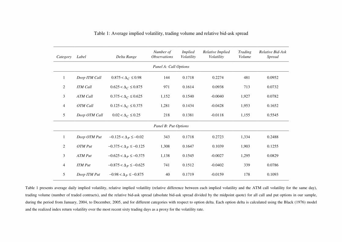
Table 1: Average implied volatility, trading volume and relative bid-ask spread

Category Label Delta Range

Number of

Observations

Implied

Volatility

Relative Implied

Volatility

Trading

Volume

Relative Bid-Ask

Spread

Panel A: Call Options

1 Deep ITM Call 98.0875.0 ≤∆< C 144 0.1718 0.2274 481 0.0952

2 ITM Call 875.0625.0 ≤∆< C 971 0.1614 0.0938 713 0.0732

3 ATM Call 625.0375.0 ≤∆< C 1,152 0.1540 -0.0040 1,927 0.0782

4 OTM Call 375.0125.0 ≤∆< C 1,281 0.1434 -0.0428 1,953 0.1652

5 Deep OTM Call 25.002.0 ≤∆< C 218 0.1381 -0.0118 1,155 0.5545

Panel B: Put Options

1 Deep OTM Put 02.0125.0 −≤∆<− P 343 0.1718 0.2723 1,334 0.2488

2 OTM Put 125.0375.0 −≤∆<− P 1,308 0.1647 0.1039 1,903 0.1255

3 ATM Put 375.0625.0 −≤∆<− P 1,138 0.1545 -0.0027 1,295 0.0829

4 ITM Put 625.0875.0 −≤∆<− P 741 0.1512 -0.0402 339 0.0786

5 Deep ITM Put 875.098.0 −≤∆<− P 40 0.1719 -0.0159 178 0.1093

Table 1 presents average daily implied volatility, relative implied volatility (relative difference between each implied volatility and the ATM call volatility for the same day),

trading volume (number of traded contracts), and the relative bid-ask spread (absolute bid-ask spread divided by the midpoint quote) for all call and put options in our sample,

during the period from January, 2004, to December, 2005, and for different categories with respect to option delta. Each option delta is calculated using the Black (1976) model

and the realized index return volatility over the most recent sixty trading days as a proxy for the volatility rate.

44

Table 2: Summary statistics for implied volatility across moneyness and option happiness

Statistic OTMPσ ATMCσ OTMCσ OTMPOH OTMCOH

Mean 0.1659 0.1505 0.1447 0.1115 -0.0382

Median 0.1620 0.1459 0.1395 0.0992 -0.0357

Maximum 0.2573 0.2537 0.2455 0.4974 0.1050

Minimum 0.1041 0.0835 0.0893 -0.0517 -0.1856

Standard Deviation 0.0338 0.0353 0.0341 0.0701 0.0350

Unit Root Test (p-value) 0.0526 0.0797 0.1940 0.0000 0.0000

Number of Observations 503 503 503 503 503

Table 2 presents summary statistics for daily implied OTM put volatility ( OTMPσ ), ATM call volatility ( ATMCσ ),

OTM call volatility ( OTMCσ ), put option happiness ( OTMPOH ), and call option happiness ( OTMCOH ) for the data

used in the regression analysis, during the period from January, 2004, to December, 2005. The augmented Dickey-

Fuller test (Fuller, 1996) is performed to test the null hypothesis that each time series has a unit root. For each series,

a MacKinnon (1996) one-sided p-value under each null hypothesis is reported.

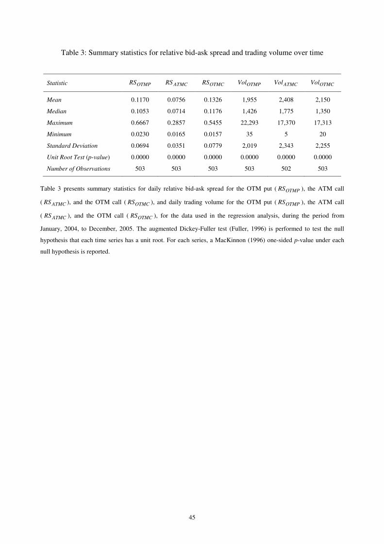
45

Table 3: Summary statistics for relative bid-ask spread and trading volume over time

Statistic OTMPRS ATMCRS OTMCRS OTMPVol ATMCVol OTMCVol

Mean 0.1170 0.0756 0.1326 1,955 2,408 2,150

Median 0.1053 0.0714 0.1176 1,426 1,775 1,350

Maximum 0.6667 0.2857 0.5455 22,293 17,370 17,313

Minimum 0.0230 0.0165 0.0157 35 5 20

Standard Deviation 0.0694 0.0351 0.0779 2,019 2,343 2,255

Unit Root Test (p-value) 0.0000 0.0000 0.0000 0.0000 0.0000 0.0000

Number of Observations 503 503 503 503 502 503

Table 3 presents summary statistics for daily relative bid-ask spread for the OTM put ( OTMPRS ), the ATM call

( ATMCRS ), and the OTM call ( OTMCRS ), and daily trading volume for the OTM put ( OTMPRS ), the ATM call

( ATMCRS ), and the OTM call ( OTMCRS ), for the data used in the regression analysis, during the period from

January, 2004, to December, 2005. The augmented Dickey-Fuller test (Fuller, 1996) is performed to test the null

hypothesis that each time series has a unit root. For each series, a MacKinnon (1996) one-sided p-value under each

null hypothesis is reported.

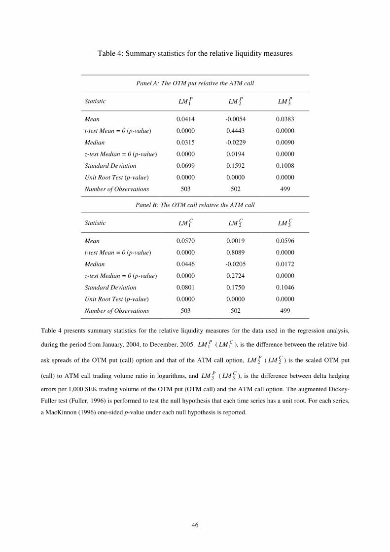
46

Table 4: Summary statistics for the relative liquidity measures

Panel A: The OTM put relative the ATM call

Statistic PLM1 PLM 2 PLM 3

Mean 0.0414 -0.0054 0.0383

t-test Mean = 0 (p-value) 0.0000 0.4443 0.0000

Median 0.0315 -0.0229 0.0090

z-test Median = 0 (p-value) 0.0000 0.0194 0.0000

Standard Deviation 0.0699 0.1592 0.1008

Unit Root Test (p-value) 0.0000 0.0000 0.0000

Number of Observations 503 502 499

Panel B: The OTM call relative the ATM call

Statistic CLM1 CLM 2 CLM 3

Mean 0.0570 0.0019 0.0596

t-test Mean = 0 (p-value) 0.0000 0.8089 0.0000

Median 0.0446 -0.0205 0.0172

z-test Median = 0 (p-value) 0.0000 0.2724 0.0000

Standard Deviation 0.0801 0.1750 0.1046

Unit Root Test (p-value) 0.0000 0.0000 0.0000

Number of Observations 503 502 499

Table 4 presents summary statistics for the relative liquidity measures for the data used in the regression analysis,

during the period from January, 2004, to December, 2005. PLM1 ( CLM1 ), is the difference between the relative bid-

ask spreads of the OTM put (call) option and that of the ATM call option, PLM 2 ( CLM 2 ) is the scaled OTM put

(call) to ATM call trading volume ratio in logarithms, and PLM 3 ( CLM 3 ), is the difference between delta hedging

errors per 1,000 SEK trading volume of the OTM put (OTM call) and the ATM call option. The augmented Dickey-

Fuller test (Fuller, 1996) is performed to test the null hypothesis that each time series has a unit root. For each series,

a MacKinnon (1996) one-sided p-value under each null hypothesis is reported.

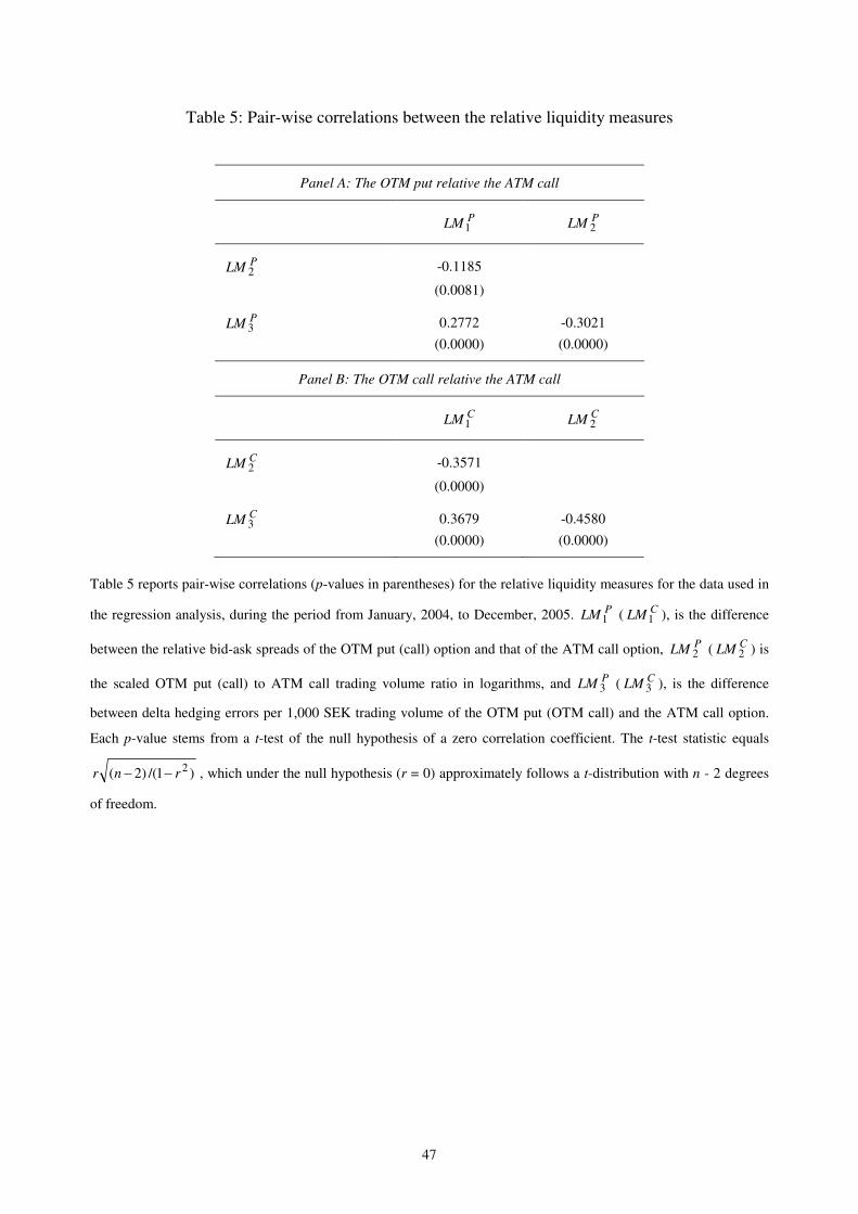
47

Table 5: Pair-wise correlations between the relative liquidity measures

Panel A: The OTM put relative the ATM call

PLM1 PLM 2

PLM 2 -0.1185

(0.0081)

PLM 3 0.2772 -0.3021

(0.0000) (0.0000)

Panel B: The OTM call relative the ATM call

CLM1 CLM 2

CLM 2 -0.3571

(0.0000)

CLM 3 0.3679 -0.4580

(0.0000) (0.0000)

Table 5 reports pair-wise correlations (p-values in parentheses) for the relative liquidity measures for the data used in

the regression analysis, during the period from January, 2004, to December, 2005. PLM1 ( CLM1 ), is the difference

between the relative bid-ask spreads of the OTM put (call) option and that of the ATM call option, PLM 2 ( CLM 2 ) is

the scaled OTM put (call) to ATM call trading volume ratio in logarithms, and PLM 3 ( CLM 3 ), is the difference

between delta hedging errors per 1,000 SEK trading volume of the OTM put (OTM call) and the ATM call option.

Each p-value stems from a t-test of the null hypothesis of a zero correlation coefficient. The t-test statistic equals

)1/()2( 2rnr −− , which under the null hypothesis (r = 0) approximately follows a t-distribution with n - 2 degrees

of freedom.

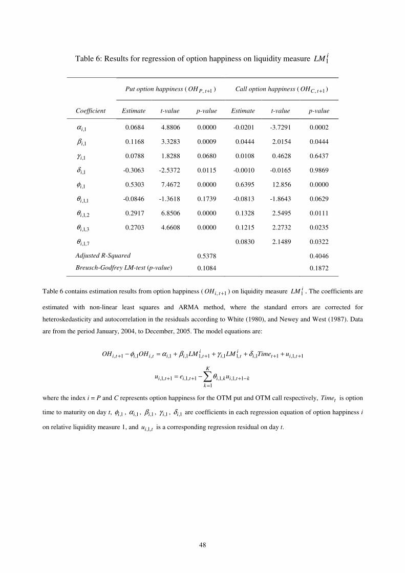
48

Table 6: Results for regression of option happiness on liquidity measure iLM1

Put option happiness ( 1, +tPOH ) Call option happiness ( 1, +tCOH )

Coefficient Estimate t-value p-value Estimate t-value p-value

1,iα 0.0684 4.8806 0.0000 -0.0201 -3.7291 0.0002

1,iβ 0.1168 3.3283 0.0009 0.0444 2.0154 0.0444

1,iγ 0.0788 1.8288 0.0680 0.0108 0.4628 0.6437

1,iδ -0.3063 -2.5372 0.0115 -0.0010 -0.0165 0.9869

1,iφ 0.5303 7.4672 0.0000 0.6395 12.856 0.0000

1,1,iθ -0.0846 -1.3618 0.1739 -0.0813 -1.8643 0.0629

2,1,iθ 0.2917 6.8506 0.0000 0.1328 2.5495 0.0111

3,1,iθ 0.2703 4.6608 0.0000 0.1215 2.2732 0.0235

7,1,iθ 0.0830 2.1489 0.0322

Adjusted R-Squared 0.5378 0.4046

Breusch-Godfrey LM-test (p-value) 0.1084 0.1872

Table 6 contains estimation results from option happiness ( 1, +tiOH ) on liquidity measure iLM1 . The coefficients are

estimated with non-linear least squares and ARMA method, where the standard errors are corrected for

heteroskedasticity and autocorrelation in the residuals according to White (1980), and Newey and West (1987). Data

are from the period January, 2004, to December, 2005. The model equations are:

1,1,11,,11,1,11,1,,1,1, ++++ ++++=− titii

tii

tiitiiti uTimeLMLMOHOH δγβαφ

∑=

−+++ −=K

k

ktikititi ueu

1

1,1,,1,1,1,1,1, θ

where the index i = P and C represents option happiness for the OTM put and OTM call respectively, tTime is option

time to maturity on day t, 1,iφ , 1,iα , 1,iβ , 1,iγ , 1,iδ are coefficients in each regression equation of option happiness i

on relative liquidity measure 1, and tiu ,1, is a corresponding regression residual on day t.

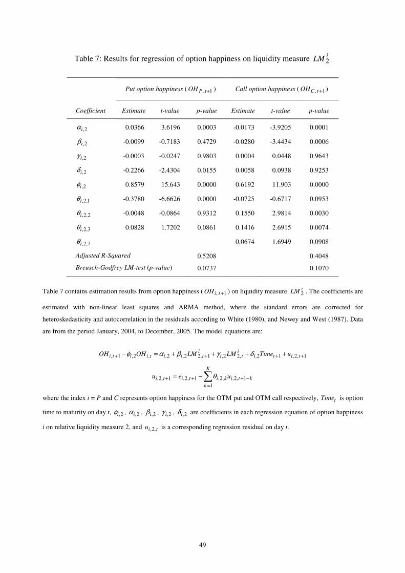
49

Table 7: Results for regression of option happiness on liquidity measure iLM 2

Put option happiness ( 1, +tPOH ) Call option happiness ( 1, +tCOH )

Coefficient Estimate t-value p-value Estimate t-value p-value

2,iα 0.0366 3.6196 0.0003 -0.0173 -3.9205 0.0001

2,iβ -0.0099 -0.7183 0.4729 -0.0280 -3.4434 0.0006

2,iγ -0.0003 -0.0247 0.9803 0.0004 0.0448 0.9643

2,iδ -0.2266 -2.4304 0.0155 0.0058 0.0938 0.9253

2,iφ 0.8579 15.643 0.0000 0.6192 11.903 0.0000

1,2,iθ -0.3780 -6.6626 0.0000 -0.0725 -0.6717 0.0953

2,2,iθ -0.0048 -0.0864 0.9312 0.1550 2.9814 0.0030

3,2,iθ 0.0828 1.7202 0.0861 0.1416 2.6915 0.0074

7,2,iθ 0.0674 1.6949 0.0908

Adjusted R-Squared 0.5208 0.4048

Breusch-Godfrey LM-test (p-value) 0.0737 0.1070

Table 7 contains estimation results from option happiness ( 1, +tiOH ) on liquidity measure iLM 2 . The coefficients are

estimated with non-linear least squares and ARMA method, where the standard errors are corrected for

heteroskedasticity and autocorrelation in the residuals according to White (1980), and Newey and West (1987). Data

are from the period January, 2004, to December, 2005. The model equations are:

1,2,12,,22,1,22,2,,2,1, ++++ ++++=− titii

tii

tiitiiti uTimeLMLMOHOH δγβαφ

∑=

−+++ −=K

k

ktikititi ueu

1

1,2,,2,1,2,1,2, θ

where the index i = P and C represents option happiness for the OTM put and OTM call respectively, tTime is option

time to maturity on day t, 2,iφ , 2,iα , 2,iβ , 2,iγ , 2,iδ are coefficients in each regression equation of option happiness

i on relative liquidity measure 2, and tiu ,2, is a corresponding regression residual on day t.

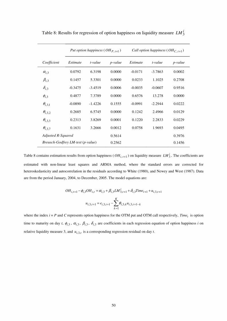
50

Table 8: Results for regression of option happiness on liquidity measure iLM3

Put option happiness ( 1, +tPOH ) Call option happiness ( 1, +tCOH )

Coefficient Estimate t-value p-value Estimate t-value p-value

3,iα 0.0792 6.3198 0.0000 -0.0171 -3.7863 0.0002

3,iβ 0.1457 5.3301 0.0000 0.0233 1.1025 0.2708

3,iδ -0.3475 -3.4519 0.0006 -0.0035 -0.0607 0.9516

3,iφ 0.4877 7.3789 0.0000 0.6576 13.278 0.0000

1,3,iθ -0.0890 -1.4226 0.1555 -0.0991 -2.2944 0.0222

2,3,iθ 0.2685 6.5745 0.0000 0.1242 2.4966 0.0129

3,3,iθ 0.2313 3.8269 0.0001 0.1220 2.2833 0.0229

7,3,iθ 0.1631 3.2666 0.0012 0.0758 1.9693 0.0495

Adjusted R-Squared 0.5614 0.3976

Breusch-Godfrey LM-test (p-value) 0.2562 0.1456

Table 8 contains estimation results from option happiness ( 1, +tiOH ) on liquidity measure iLM 3 . The coefficients are

estimated with non-linear least squares and ARMA method, where the standard errors are corrected for

heteroskedasticity and autocorrelation in the residuals according to White (1980), and Newey and West (1987). Data

are from the period January, 2004, to December, 2005. The model equations are:

1,3,13,1,33,3,,3,1, ++++ +++=− titii

tiitiiti uTimeLMOHOH δβαφ

∑=

−+++ −=K

k

ktikititi ueu

1

1,3,,3,1,3,1,3, θ

where the index i = P and C represents option happiness for the OTM put and OTM call respectively, tTime is option

time to maturity on day t, 3,iφ , 3,iα , 3,iβ , 3,iδ are coefficients in each regression equation of option happiness i on

relative liquidity measure 3, and tiu ,3, is a corresponding regression residual on day t.

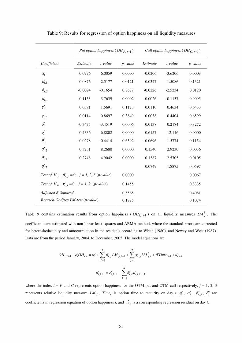
51

Table 9: Results for regression of option happiness on all liquidity measures

Put option happiness ( 1, +tPOH ) Call option happiness ( 1, +tCOH )

Coefficient Estimate t-value p-value Estimate t-value p-value

iα ′ 0.0776 6.0059 0.0000 -0.0206 -3.6206 0.0003

1,iβ ′ 0.0876 2.5177 0.0121 0.0347 1.5086 0.1321

2,iβ ′ -0.0024 -0.1654 0.8687 -0.0226 -2.5234 0.0120

3,iβ ′ 0.1153 3.7639 0.0002 -0.0026 -0.1137 0.9095

1,iγ ′ 0.0581 1.5691 0.1173 0.0110 0.4634 0.6433

2,iγ ′ 0.0114 0.8697 0.3849 0.0038 0.4404 0.6599

iδ ′ -0.3475 -3.4519 0.0006 0.0138 0.2184 0.8272

iφ ′ 0.4336 6.8802 0.0000 0.6157 12.116 0.0000

1,iθ ′ -0.0278 -0.4414 0.6592 -0.0696 -1.5774 0.1154

2,iθ ′ 0.3251 8.2680 0.0000 0.1540 2.9230 0.0036

3,iθ ′ 0.2748 4.9042 0.0000 0.1387 2.5705 0.0105

7,iθ ′ 0.0749 1.8875 0.0597

Test of 3H : 0, =′ jiβ , j = 1, 2, 3 (p-value) 0.0000 0.0067

Test of 4H : 0, =′ jiγ , j = 1, 2 (p-value) 0.1455 0.8335

Adjusted R-Squared 0.5565 0.4081

Breusch-Godfrey LM-test (p-value) 0.1825 0.1074

Table 9 contains estimation results from option happiness ( 1, +tiOH ) on all liquidity measures ijLM . The

coefficients are estimated with non-linear least squares and ARMA method, where the standard errors are corrected

for heteroskedasticity and autocorrelation in the residuals according to White (1980), and Newey and West (1987).

Data are from the period January, 2004, to December, 2005. The model equations are:

1,1

2

1

,,

3

1

1,,,1, ++

==

++ ′+′+′+′+′=′− ∑∑ titi

j

itjji

j

itjjiitiiti uTimeLMLMOHOH δγβαφ

∑=

−+++ ′′−′=′K

k

ktikititi ueu

1

1,,1,1, θ

where the index i = P and C represents option happiness for the OTM put and OTM call respectively, j = 1, 2, 3

represents relative liquidity measure jLM , tTime is option time to maturity on day t, iφ ′ , iα ′ , ji,β ′ , iδ ′ are

coefficients in regression equation of option happiness i, and tiu ,′ is a corresponding regression residual on day t.

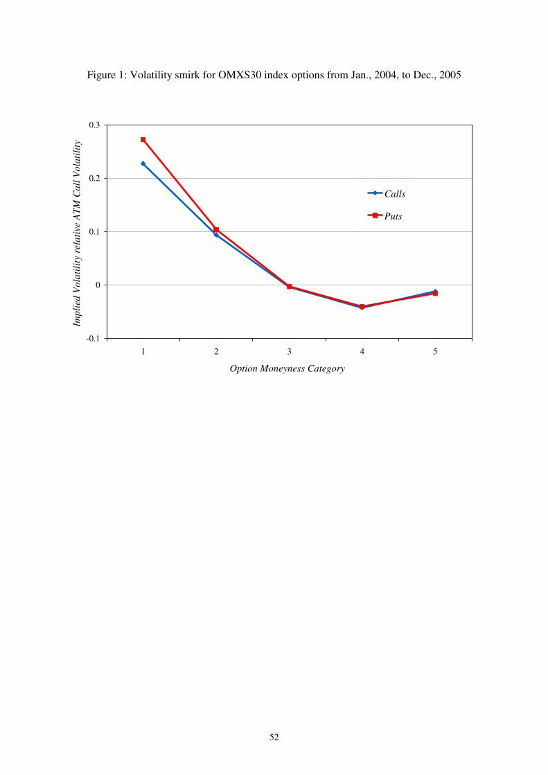
52

Figure 1: Volatility smirk for OMXS30 index options from Jan., 2004, to Dec., 2005

-0.1

0

0.1

0.2

0.3

1 2 3 4 5

Option Moneyness Category

Impli

ed V

ola

tili

ty r

ela

tive

AT

M C

all

Vola

tili

ty

Calls

Puts

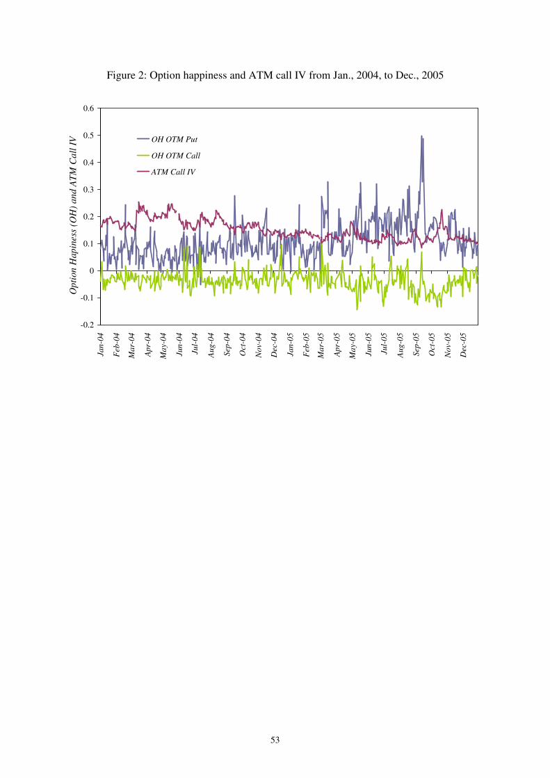
53

Figure 2: Option happiness and ATM call IV from Jan., 2004, to Dec., 2005

-0.2

-0.1

0

0.1

0.2

0.3

0.4

0.5

0.6Ja

n-0

4

Feb

-04

Mar-

04

Apr-

04

Ma

y-04

Jun-0

4

Jul-

04

Aug-0

4

Sep

-04

Oct

-04

No

v-04

Dec

-04

Jan-0

5

Feb

-05

Mar-

05

Apr-

05

Ma

y-05

Jun-0

5

Jul-

05

Aug-0

5

Sep

-05

Oct

-05

No

v-05

Dec

-05

Op

tion

Hap

ines

s (O

H)

an

d A

TM

Ca

ll I

V OH OTM Put

OH OTM Call

ATM Call IV