Embed Size (px)
DESCRIPTION
Option Pricing. Downloads. Today’s work is in: matlab_lec08.m Functions we need today: pricebinomial.m, pricederiv.m. Derivatives. A derivative is any security the payout of which fully depends on another security Underlying is the security on which a derivative’s value depends - PowerPoint PPT Presentation
Citation preview

Option Pricing

Downloads
Today’s work is in: matlab_lec08.m
Functions we need today: pricebinomial.m, pricederiv.m
Derivatives
A derivative is any security the payout of which fully depends on another security
Underlying is the security on which a derivative’s value depends
European Call gives owner the option to buy the underlying at expiry for the strike price
European Put gives owner the option to sell the underlying at expiry for the strike price

Binomial Tree

Arbitrage Pricing (1 period)
Lets make a portfolio that exactly replicates underlying payoff, buy Δ shares of stock, and B dollars of bond
CH = B*Rf+ΔPS(1+σ) CL = B*Rf+ΔPS(1-σ) Solve for B and Δ: Δ=(CH-CL)/(2σPS) and B=(CH-ΔPS(1+σ))/Rf PU= ΔPS+B

pricebinomial.m
function out=pricebinomial(pS,Rf,sigma,Ch,Cl);
D=(Ch-Cl)/(pS*2*sigma);B=(Ch-(1+sigma)*pS*D)/Rf;pC=B+pS*D;out=[pC D];

Price Call
Suppose the price of the underlying is 100 and the volatility is 10%; suppose the risk free rate is 2%
The payoff of a call with strike 100 is 10 in the good state and 0 in the bad state: C=max(P-X,0)
What is the price of this call option?>>pS=100; Rf=1.02; sigma=.1; Ch=10; Cl=0;>>pricebinomial(pS,Rf,sigma,Ch,Cl) Price=5.88, Δ=.5
Larger Trees
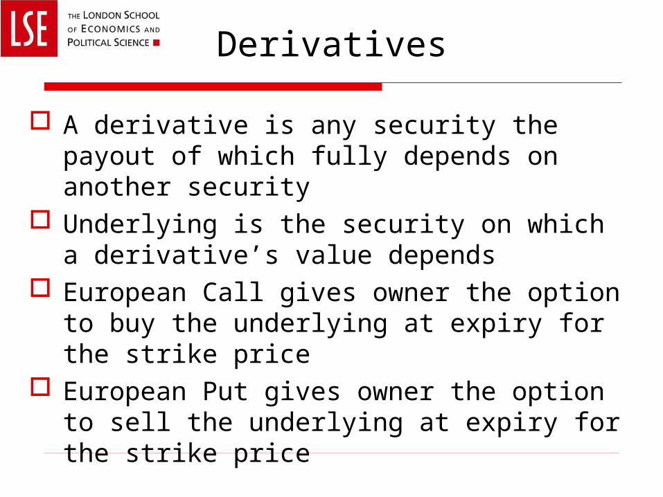
The assumption that the world only has two states is unrealistic
However its not unrealistic to assume that the price in one minute can only take on two values
This would imply that in one day, week, year, etc. there are many possible prices, as in the real world
In fact, at the limit, the binomial assumption implies a log-normal distribution of prices at expiry

Binomial Tree (multiperiod)

Tree as matrix
100.0000 108.0000 116.6400 125.9712 0 92.0000 99.3600 107.3088 0 0 99.3600 107.3088 0 0 84.6400 91.4112 0 0 0 107.3088 0 0 0 91.4112 0 0 0 91.4112 0 0 0 77.8688

Prices of Underlying
Recursively define prices forward>>N=3; P=zeros(2^N,N+1);%create a price grid for underlying>>P(1,1)=pS; for i=1:N; for j=1:2^(i-1); P((j-1)*2+1,i+1)=P(j,i)*(1+sigma); P((j-1)*2+2,i+1)=P(j,i)*(1-sigma); %disp([i j i+1 (j-1)*2+1 (j-1)*2+2]); end; end;

Indexing
disp([i j i+1 (j-1)*2+1 (j-1)*2+2]);
1 1 2 1 2 2 1 3 1 2 2 2 3 3 4 3 1 4 1 2 3 2 4 3 4 3 3 4 5 6 3 4 4 7 8

Payout at Expiry
Payout of derivative at expiry is a function of the underlying
European Call: C(:,N+1)=max(P(:,N+1)-X,0); European Put: C(:,N+1)=max(X-P(:,N+1),0); This procedure can price any derivative, as
long as we can define its payout at expiry as a function of the underlying
For example C(:,N+1)=abs(P(:,N+1)-X); would be a type of volatility hedge

Payout at Expiry

Prices of DerivativeRecursively define prices backwards>>X=100; C(:,N+1)=max(P(:,N+1)-X,0); %call option >>for k=1:N; i=N+1-k; for j=1:2^(i-1); Ch=C((j-1)*2+1,i+1); Cl=C((j-1)*2+2,i+1); pStemp=P(j,i); out=pricebinomial(pStemp,Rf,sigma,Ch,Cl); C(j,i)=out(1); %disp([i j i+1 (j-1)*2+1 (j-1)*2+2]); end; end;

Indexing
>>disp([i j i+1 (j-1)*2+1 (j-1)*2+2]);
3 1 4 1 2 3 2 4 3 4 3 3 4 5 6 3 4 4 7 8 2 1 3 1 2 2 2 3 3 4 1 1 2 1 2

pricederiv.m
function out=pricederiv(pS,Rf,sigmaAgg,X,N)sigma=sigmaAgg/sqrt(N); Rf=Rf^(1/N); %define sigma, Rf for shorter periodC=zeros(2^N,N+1); P=zeros(2^N,N+1); %initialize price vectorsP(1,1)=pS;for i=1:N; %create price grid for underlying for j=1:2^(i-1); P((j-1)*2+1,i+1)=P(j,i)*(1+sigma); P((j-1)*2+2,i+1)=P(j,i)*(1-sigma); end;end;C(:,N+1)=max(P(:,N+1)-X,0); %a european call for k=1:N; %create price grid for option i=N+1-k; for j=1:2^(i-1); Ch=C((j-1)*2+1,i+1); Cl=C((j-1)*2+2,i+1); pStemp=P(j,i); x=pricebinomial(pStemp,Rf,sigma,Ch,Cl); C(j,i)=x(1); end;end;out=C(1,1);

Investigating N
>>pS=100; Rf=1.02; sigmaAgg=.3; X=100; B-S value of this call is 12.8
http://www.blobek.com/black-scholes.html >>for N=1:15; out(N,1)=N; out(N,2)=pricederiv(pS,Rf,sigmaAgg,X,N); end;>>plot(out(:,1),out(:,2)); This converges to B-S as N grows!

Convergence to B-S Price

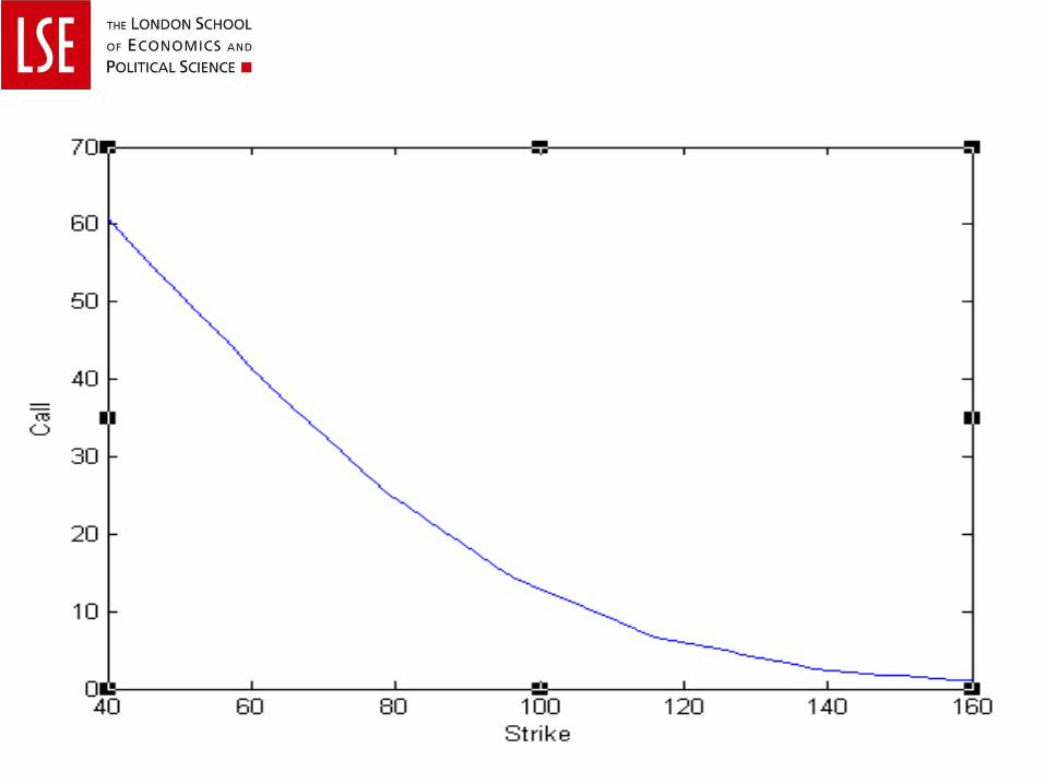
Investigating Strike Price
>>pS=100; Rf=1.02; sigmaAgg=.3; N=10;>>for i=1:50; X=40+120*(i-1)/(50-1); out(i,1)=X; out(i,2)=pricederiv(pS,Rf,sigmaAgg,X,N); end;>>plot(out(:,1),out(:,2));>>xlabel('Strike'); ylabel('Call');

InvestigatingUnderlying Price
>>X=100; Rf=1.02; sigmaAgg=.3; N=10;>>for i=1:50; pS=40+120*(i-1)/(50-1); out(i,1)=pS; out(i,2)=pricederiv(pS,Rf,sigmaAgg,X,N); end;>>plot(out(:,1),out(:,2));>>xlabel('Price'); ylabel('Call');


Investigating sigma
>>X=100; Rf=1.02; pS=100; N=10;>>for i=1:50; sigmaAgg=.01+.8*(i-1)/(50-1); out(i,1)=sigmaAgg; out(i,2)=pricederiv(pS,Rf,sigmaAgg,X,N); end;>>plot(out(:,1),out(:,2));>>xlabel('Sigma'); ylabel('Call');