Option Valuation Fft

8/3/2019 Option Valuation Fft

http://slidepdf.com/reader/full/option-valuation-fft 1/13

Option valuation using the fast Fourier transformPeter Carr and Dilip B. Madan

In this paper the authors show how the fast Fourier transform may be used to value

options when the characteristic function of the return is known analytically.

1. INTRODUCTION

The Black±Scholes model and its extensions comprise one of the major develop-

ments in modern ®nance. Much of the recent literature on option valuation has

successfully applied Fourier analysis to determine option prices (see e.g. Bakshi

and Chen 1997, Scott 1997, Bates 1996, Heston 1993, Chen and Scott 1992).

These authors numerically solve for the delta and for the risk-neutral prob-

ability of ®nishing in-the-money, which can be easily combined with the stock

price and the strike price to generate the option value. Unfortunately, this

approach is unable to harness the considerable computational power of the fast

Fourier transform (FFT) (Walker 1996), which represents one of the most

fundamental advances in scienti®c computing. Furthermore, though the decom-

position of an option price into probability elements is theoretically attractive, asexplained by Bakshi and Madan (1999), it is numerically undesirable owing to

discontinuity of the payos.

The purpose of this paper is to describe a new approach for numerically

determining option values, which is designed to use the FFT to value options

eciently. As is the case with all of the above approaches, our technique

assumes that the characteristic function of the risk-neutral density is known

analytically. Given any such characteristic function, we develop a simple

analytic expression for the Fourier transform of the option value or its time

value. We then use the FFT to numerically solve for the option price or its

time value. Our use of the FFT in the inversion stage permits real-time pricing,

marking, and hedging using realistic models, even for books with thousands of options.

To test the accuracy of our approach, we would like to use a model where the

option price is known analytically. To illustrate the potential power of Fourier

analysis, we would also like to use a model in which the density function is

complicated, while the characteristic function of the log price is simple. Finally,

we would like to use a model which is supported in a general equilibrium and

which is capable of removing the biases of the standard Black±Scholes model.

All of these requirements are met by the variance gamma (VG) model, which

assumes that the log price obeys a one-dimensional pure jump Markov process

with stationary independent increments. The mathematics of this process is

detailed by Madan and Seneta (1990), while the economic motivation and

61



empirical support for this model is described by Madan and Milne (1991) and

by Madan, Carr, and Chang (1998) respectively.The outline of this paper is as follows. In Section 2, we brie¯y review the

current literature on the use of Fourier methods in option pricing. In Section 3,

we present our approach for analytically determining the Fourier transform of

the option value and of the time value in terms of the characteristic function of

the risk-neutral density. Section 4 details the use of the FFT to numerically solve

for the option price or time value. In Section 5, we illustrate our approach in the

VG model. Section 6 concludes.

2. REVIEW OF FOURIER METHODS IN OPTION PRICING

Consider the problem of valuing a European call of maturity T, written on the

terminal spot price ST of some underlying asset. The characteristic function of

sT lnST is de®ned by

0Tu EexpiusTX 1

In many situations this characteristic function is known analytically. A wide

class of examples arises when the the dynamics of the log price is given by an

in®nitely divisible process of independent increments. The characteristic func-

tion then arises naturally from the Le Â vy±Khintchine representation for such

processes. Among this class of processes, we have the process of independent

stable increments (McCulloch 1978), the VG process (Madan, Carr, and Chang1998), the inverse Gaussian law (Barndor-Nielsen 1997), and a wide range of

other processes proposed by Geman, Yor, and Madan (1998). Characteristic

functions have also been used in the pure diusion context with stochastic

volatility (Heston 1993) and with stochastic interest rates (Bakshi and Chen

1997). Finally, they have been used for jumps coupled with stochastic volatility

(Bates 1996) and for jumps coupled with stochastic interst rates and volatility

(Scott 1997). The solution methods can also be applied to average rate claims

and to other exotic claims (Bakshi and Madan 1999). The methods are generally

much faster than ®nite dierence solutions to partial dierential equations or

integrodierential equations, which led Heston (1993) to refer to them as closed-

form solutions.

Assuming that the characteristic function is known analytically, many

authors (e.g. Bakshi and Madan 1999, Scott 1997) have numerically determined

the risk-neutral probability of ®nishing in-the-money as

PrST b K Å2 12

1

%

I0

Re

eÀiu lnK 0Tu

iu

duX

Similarly, the delta of the option, denoted Å1, is numerically obtained as

Å1

1

2 1

%

I

0 ReeÀiu lnK0T

u

Ài

iu0TÀi du

X

Journal of Computational Finance

P. Carr and D. B. Madan62



Assuming no dividends and constant interest rates r, the initial option value is

then determined as

C SÅ1 À KeÀrTÅ2X

Unfortunately, the FFT cannot be used to evaluate the integral, since the

integrand is singular at the required evaluation point u 0. Given the

considerable speed advantages of the FFT, we examine two alternative

approaches in the next section, both of which are amenable to evaluation by

the FFT.

3. TWO NEW FOURIER METHODS

In this section, we develop analytic expressions for the Fourier transform of an

option price and for the Fourier transform of the time value of an option. Both

Fourier transforms are expressed in terms of the characteristic function of the

log price.

3.1 The Fourier Transform of an Option Price

Let k denote the log of the strike price K, and let CTk be the desired value of a

T-maturity call option with strike expk. Let the risk-neutral density of the log

price sT be qT

s

. The characteristic function of this density is de®ned by

0Tu I

ÀIeiusqTs dsX 2

The initial call value CTk is related to the risk-neutral density qTs by

CTk Ik

eÀrTes À ekqTs dsX

Note that CT

k

tends to S0 as k tends to

ÀI, and hence the call pricing

function is not square-integrable. To obtain a square-integrable function, we

consider the modi®ed call price cTk de®ned by

cTk expkCTk 3

for b 0. For a range of positive values of , we expect that cTk is square-

integrable in k over the entire real line. We comment later on the choice of .

Consider now the Fourier transform of cTk de®ned by

2 Tv I

ÀI e

ivk

cTk dkX 4 Volume 2/Number 4, Summer 1999

Option valuation using the fast Fourier transform 63



We ®rst develop an analytical expression for 2 T

v

in terms of 0T and then

obtain call prices numerically using the inverse transform

CTk expÀk2%

IÀI

eÀivk2 Tv dv expÀk%

I0

eÀivk2 v dvX 5

The second equality holds because CTk is real, which implies that the

function 2 Tv is odd in its imaginary part and even in its real part. The

expression for 2 Tv is determined as follows:

2 Tv I

ÀI

eivk

Ik

ekeÀrTes À ekqTs ds dk

I

ÀIeÀrTqTs

sÀI

esk À e1keivk dkds

I

ÀIeÀrTqTs

e1ivs

ivÀ e1ivs

1 iv

ds

eÀrT0T

Àv À 1i

Á2 À v2 i2 1v X 6

Call values are determined by substituting (6) into (5) and performing the

required integration. We note that the integration (5) is a direct Fourier

transform and lends itself to an application of the FFT. We also note that if 0 then the denominator vanishes when v 0, inducing a singularity in the

integrand. Since the FFT evaluates the integrand at v 0, the use of the factor

expk or something similar is required.

We now consider the issue of the appropriate choice of the coecient .

Positive values of assist the integrability of the modi®ed call value over the

negative log strike axis, but aggravate the same condition for the positive log

strike axis. For the modi®ed call value to be integrable in the positive log strike

direction, and hence for it to be square-integrable as well, a sucient condition

is provided by 2 0 being ®nite. From (6), we observe that 2 T0 is ®nite

provided that 0TÀÀ

1

iÁ is ®nite. From the de®nition of the characteristic

function, this requires that

ES1T ` IX 7

In practice, one may determine an upper bound on from the analytical

expression for the characteristic function and the condition (7). We ®nd that one

quarter of this upper bound serves as a good choice for .

We now consider the issue of the in®nite upper limit of integration in (5).

Note that, since the modulus of 0t is bounded by ES1T , which is independent

of v, it follows that

2 T

v

2T

E

S1T

2 À v22 2 12v2TA

v4





for some constant A, or that

2 v `

A

p

v2X

It follows that we may bound the integral of the upper tail by

Ia

2 v dv `

A

p

aX 8

This bound makes it possible to set up a truncation procedure. Speci®cally, the

integral of the tail in computing the transform of (5) is bounded by Ap

aa, and

hence the truncation error is bounded by

expÀk%

A

p

aY

which can be made smaller than 4 by choosing

a bexpÀk

%

A

p

4X

3.2 Fourier Transform of Out-of-the-Money Option Prices

In the last section we multiplied call values by an exponential function to obtaina square-integrable function whose Fourier transform is an analytic function of

the characteristic function of the log price. Unfortunately, for very short

maturities, the call value approaches its nonanalytic intrinsic value causing

the integrand in the Fourier inversion to be highly oscillatory, and therefore

dicult to integrate numerically. The purpose of this section is to introduce an

alternative approach that works with time values only. Again letting k denote

the log of the strike and S0 denote the initial spot price, we let zTk be the T-

maturity put price when k ` lnS0Y and we let it be the T-maturity call price

when k b lnS0X For any unimodal probability density function, the function

zTk

peaks at k

ln

S0

and declines in both directions as k tends to positive or

negative in®nity. In this section, we develop an analytic expression for the

Fourier transform of zTk in terms of the characteristic function of the log of

the terminal stock price.

Let Tv denote the Fourier transform of zTk:

Tv I

ÀIeivkzTk dkX 9

The prices of out-of-the-money options are obtained by inverting this transform:

zTk 1

2%

I

ÀI eÀivk

Tv dvX 10 Volume 2/Number 4, Summer 1999




For ease of notation, we will derive T

v

assuming that S0

1 (one may

always scale up to other values later). We may then de®ne zTk by

zTk eÀrT

IÀI

ek À es1s`kYk`0 es À ek1sbkYkb0qTs dsX 11

The expression for Tv follows on noting that

Tv 0

ÀIeivkeÀrT

kÀI

ek À esqTs ds dk

I

0

eivkeÀrT

Ik

es À ekqTs ds dkX 12

Reversing the order of integration in (12) yields

Tv 0

ÀIeÀrTqTs

Is

e1ivk À eseivk dk ds

I

0

eÀrTqTs s

0

eseivk À e1ivk dk dsX 13

Performing the inner integrations, simplifying, and writing the outer integration

in terms of characteristic functions, we get

Tv eÀrT

1

1 ivÀ erT

ivÀ 0Tv À i

v2 À iv

X 14

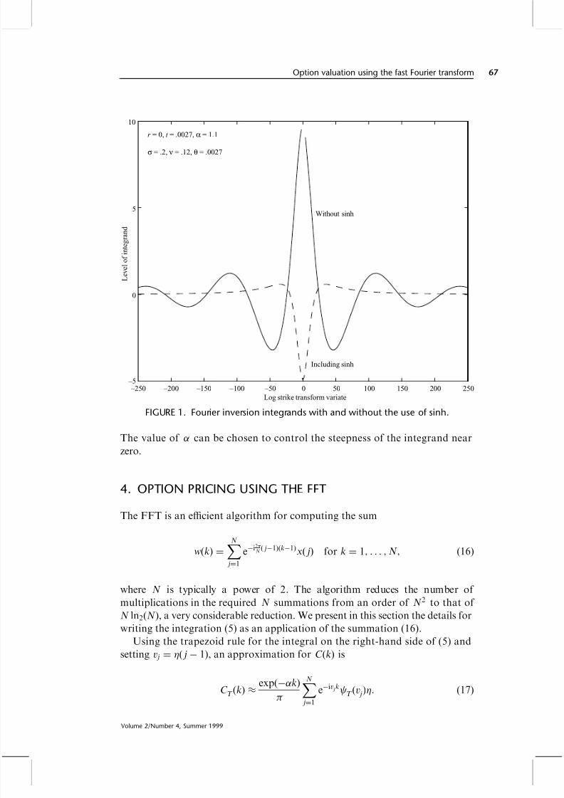
Although there is no issue regarding the behavior of zTk as k tends to

positive or negative in®nity, the time value at k 0 can get quite steep as T 3 0,

and this can cause diculties in the inversion. The function zTk approximates

the shape of a Dirac delta function near k 0 when maturity is small (see

Figure 1), and thus the transform is wide and oscillatory.

It is useful in this case to consider the transform of sinh kzTk as this

function vanishes at k 0. De®ne

Tv IÀI

eivk sinhkzTk dk

IÀI

eivk ek À eÀk

2zTk dk

Tv À i À Tv i2

X 15

Thus, the time value is given by

zTk 1

sinhk1

2%

I

ÀI eÀivk

Tv dvX





The value of can be chosen to control the steepness of the integrand near

zero.

4. OPTION PRICING USING THE FFT

The FFT is an ecient algorithm for computing the sum

w

k

N

j1

eÀi2%N jÀ1kÀ1x

j

for k

1Y F F F YNY

16

where N is typically a power of 2. The algorithm reduces the number of

multiplications in the required N summations from an order of N2 to that of

N ln2N, a very considerable reduction. We present in this section the details for

writing the integration (5) as an application of the summation (16).

Using the trapezoid rule for the integral on the right-hand side of (5) and

setting v j j À 1, an approximation for Ck is

CT

k

%expÀk

%N

j1

eÀiv jk2 Tv j

X

17

–250 –200 –150 –100 –50 0 50 100 150 200 250 –5

0

5

10

Log strike transform variate

L

e v e l o f i n t e g r a n d

Without sinh

Including sinh

r = 0, t = .0027, α = 1.1

σ = .2, ν = .12, θ = .0027

FIGURE 1. Fourier inversion integrands with and without the use of sinh.

Volume 2/Number 4, Summer 1999




The eective upper limit for the integration is now

a NX 18

We are mainly interested in at-the-money call values Ck, which correspond

to k near 0. The FFT returns N values of k and we employ a regular spacing of

size !, so that our values for k are

ku Àb !u À 1 for u 1Y F F F YNX 19

This gives us log strike levels ranging from Àb to b, where

b 12N!X 20

Substituting (19) into (17) yields

CTku % expÀku%

N j1

eÀiv jÀb!uÀ12 Tv j for u 1Y F F F YNX 21

Noting that v j j À 1, we write

CTku % expÀku%

N j1

eÀi! jÀ1uÀ1eibv j2 Tv jX 22

To apply the fast Fourier transform, we note from (16) that

! 2%

NX 23

Hence, if we choose small in order to obtain a ®ne grid for the integration,

then we observe call prices at strike spacings that are relatively large, with few

strikes lying in the desired region near the stock price. We would therefore like to

obtain an accurate integration with larger values of and, for this purpose, we

incorporate Simpson's rule weightings into our summation. With Simpson's rule

weightings and the restriction (23), we may write our call price as

Cku expÀku%

N j1

eÀi2%N

jÀ1uÀ1eibv j2 v j 3

3 À1 j À jÀ1Y 24

where n is the Kronecker delta function that is unity for n 0 and zero

otherwise. The summation in (24) is an exact application of the FFT. One

needs to make the appropriate choices for and . The next section addresses

these issues in the context of the VG option pricing model used to illustrate our

approaches.

The use of the FFT for calculating out-of-the-money option prices is similar

to (24). The only dierences are that we replace the multiplication by expÀkuwith a division by sinh

k

and the function call to 2

v

is replaced by a function

call to v de®ned in (15).





5. THE FFT FOR VG OPTION PRICING

The VG option pricing model is described in detail in Madan, Carr, and Chang

(1998), who document that this process eectively removes the smile observed

when plotting Black±Scholes implied volatilities against strike prices. The VG

process is obtained by evaluating arithmetic Brownian motion with drift and

volatility ' at a random time given by a gamma process having a mean rate per

unit time of 1 and a variance rate of #. The resulting process Xt' Y Y # is a pure

jump process with two additional parameters and # relative to the Black±

Scholes model, providing control over skewness and kurtosis respectively. The

resulting risk-neutral process for the stock price is

St S0 exprt Xt' Y Y # 3tY t b 0Y 25where, by setting 3 1a# ln1 À # À 1

2 ' 2#, the mean rate of return on the

stock equals the interest rate r.

Madan, Carr, and Chang (1998) show that the characteristic function for the

log of ST is

0Tu explnS0 r 3T1 À i#u 12 ' 2u2#ÀTa#

X 26

To obtain option prices, one can analytically invert this characteristic function

to get the density function, and then integrate the density function against the

option payo. Madan, Carr, and Chang (1998) provide a closed-form formula

for both the density function and the option price. Alternatively, the Fouriertransform of the distribution functions can be numerically inverted as reviewed

in Section 1. Finally, the Fourier transform of the modi®ed call can be

numerically inverted without using FFT. In this last case, one must set the

damping coecient . To accomplish this, we evaluate the term 0T

ÀÀ 1iÁ

in

(7) as

0T

ÀÀ 1iÁ explnS0 r 3T1 À # 1 À 1

2 ' 2 12#ÀTa#X

For this expression to be ®nite, we must have

`

2

' 4 2

' 2#

r À

' 2À 1X

Generally, we anticipate in our estimates that the expectation of S2T is ®nite and

that this upper bound is above unity. A value of above unity and well below

the upper bound performs well.

For our FFT methods, we found that setting the spacing 0X25 delivers the

speedup of the FFT without compromising the accuracy delivered by other

methods. However, as a quality control, we recommend selective checking of the

FFT output against other methods. We used N 4096 points in our quad-

rature, implying a log strike spacing of 8%a4096

X00613, or a little over half a

percentage point, which is adequate for practice. For the choice of the





dampening coecient in the transform of the modi®ed call price, we used a

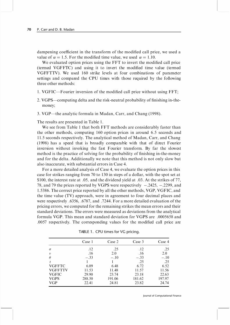
value of 1X5. For the modi®ed time value, we used 1X10.We evaluated option prices using the FFT to invert the modi®ed call price

(termed VGFFTC) and using it to invert the modi®ed time value (termed

VGFFTTV). We used 160 strike levels at four combinations of parameter

settings and compared the CPU times with those required by the following

three other methods:

1. VGFICÐFourier inversion of the modi®ed call price without using FFT;

2. VGPSÐcomputing delta and the risk-neutral probability of ®nishing in-the-

money;

3. VGPÐthe analytic formula in Madan, Carr, and Chang (1998).

The results are presented in Table 1.

We see from Table 1 that both FFT methods are considerably faster than

the other methods, computing 160 option prices in around 6X5 seconds and

11X5 seconds respectively. The analytical method of Madan, Carr, and Chang

(1998) has a speed that is broadly comparable with that of direct Fourier

inversion without invoking the fast Fourier transform. By far the slowest

method is the practice of solving for the probability of ®nishing in-the-money

and for the delta. Additionally we note that this method is not only slow but

also inaccurate, with substantial errors in Case 4.

For a more detailed analysis of Case 4, we evaluate the option prices in thiscase for strikes ranging from 70 to 130 in steps of a dollar, with the spot set at

6100, the interest rate at X05Y and the dividend yield at X03. At the strikes of 77,

78, and 79 the prices reported by VGPS were respectively ÀX2425, ÀX2299, and

1X5386. The correct price reported by all the other methods, VGP, VGFIC, and

the time value (TV) approach, were in agreement to four decimal places and

were respectively X6356, X6787, and X7244. For a more detailed evaluation of the

pricing errors, we computed for the remaining strikes the mean errors and their

standard deviations. The errors were measured as deviations from the analytical

formula VGP. This mean and standard deviation for VGPS are X0005658 and

X0057 respectively. The corresponding values for the modi®ed call price are

TABLE 1. CPU times for VG pricing.

Case 1 Case 2 Case 3 Case 4

' .12 .25 .12 .25# .16 2.0 .16 2.0 À.33 À.10 À.33 À.10t 1 1 .25 .25VGFFTC 6.09 6.48 6.72 6.52VGFFTTV 11.53 11.48 11.57 11.56VGFIC 29.90 23.74 23.18 22.63VGPS 288.50 191.06 181.62 197.97

VGP 22.41 24.81 23.82 24.74





X0001196 and X0041, while for the time value approach we have X000006059 and

X0002662. Hence, we observe that the time value approach is an order of

magnitude lower in its pricing errors compared with VGFIC, which is

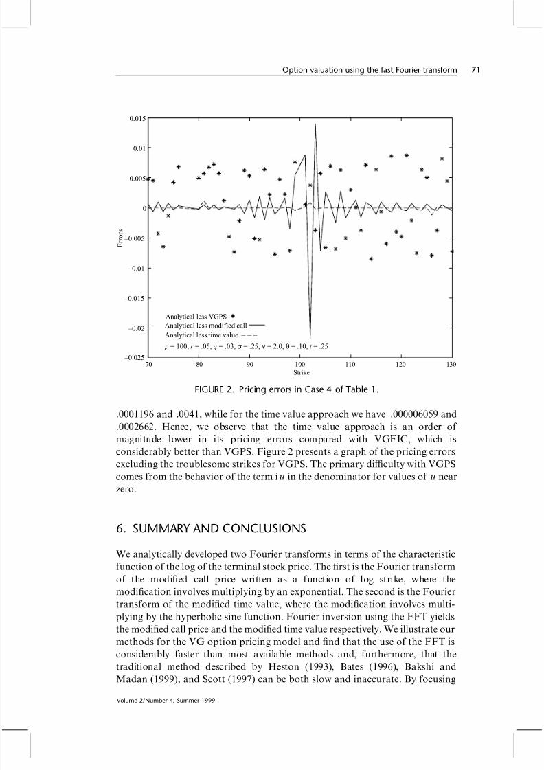
considerably better than VGPS. Figure 2 presents a graph of the pricing errors

excluding the troublesome strikes for VGPS. The primary diculty with VGPS

comes from the behavior of the term iu in the denominator for values of u near

zero.

6. SUMMARY AND CONCLUSIONS

We analytically developed two Fourier transforms in terms of the characteristic

function of the log of the terminal stock price. The ®rst is the Fourier transform

of the modi®ed call price written as a function of log strike, where the

modi®cation involves multiplying by an exponential. The second is the Fourier

transform of the modi®ed time value, where the modi®cation involves multi-

plying by the hyperbolic sine function. Fourier inversion using the FFT yields

the modi®ed call price and the modi®ed time value respectively. We illustrate our

methods for the VG option pricing model and ®nd that the use of the FFT is

considerably faster than most available methods and, furthermore, that the

traditional method described by Heston (1993), Bates (1996), Bakshi and

Madan (1999), and Scott (1997) can be both slow and inaccurate. By focusing

70 80 90 100 110 120 130 –0.025

–0.02

–0.015

–0.01

–0.005

0

0.005

0.01

0.015

Strike

E r r o r s

Analytical less VGPS

Analytical less modified call

Analytical less time value

p = 100, r = .05, q = .03, σ = .25, ν = 2.0, θ = .10, t = .25

FIGURE 2. Pricing errors in Case 4 of Table 1.





attention on delta claims, the traditional method sacri®ces the advantages of the

continuity of the call payo and inherits in its place the problematic discontinu-ity of these claims. Thus, we recommend the use of the VGFFTC or VGFFTTV

and in general the use of the FFT whenever the characteristic function of the

underlying uncertainty is available in closed form.

We anticipate that the advantages of the FFT are generic to the widely known

improvements in computation speed attained by this algorithm and is not

connected to the particular characteristic function or process we chose to

analyze. We have observed similar speed improvements when we work with

generalizations of the VG model introduced by Geman, Madan, and Yor

(1998), where a considerable variety of processes are developed with closed

forms for the characteristic function of the log price.

REFERENCESREFERENCES

Bakshi, G., and Chen, Z. (1997). An alternative valuation model for contingent claims.

Journal of Financial Economics, 44(1), 123±165.

Bakshi, G., and Madan, D. B. (1999). Spanning and derivative security valuation.

Forthcoming in: Journal of Financial Economics.

Barndor-Nielsen, O. E. (1997). Processes of normal inverse Gaussian type. Finance and

Stochastics, 2, 41±68.

Bates, D. (1996). Jumps and stochastic volatility: Exchange rate processes implicit in

Deutschemark options. Review of Financial Studies, 9, 69±108.

Black, F., and Scholes, M. (1973). The pricing of options and corporate liabilities.

Journal of Political Economy, 81, 637±659.

Chen, R.-R., and Scott, L. (1992). Pricing interest rate options in a two-factor Cox±

Ingersoll±Ross model of the term structure. Review of Financial Studies, 5, 613±636.

Geman, H., Madan, D., and Yor, M. (1998). Asset prices are Brownian motion: Only in

business time. Working paper, University of Maryland, College Park, Maryland.

Heston, S. (1993). A closed-form solution for options with stochastic volatility with

applicatons to bond and currency options. Review of Financial Studies, 6, 327±343.

Madan, D. B., Carr, P., and Chang, E. C. (1998). The variance gamma process and

option pricing. European Finance Review, 2, 79±105.

Madan, D. B., and Milne, F. (1991). Option pricing with VG martingale components.

Mathematical Finance, 1, 39±55.

Madan, D. B., and Seneta, E. (1990). The variance gamma (V.G.) model for share

market returns. Journal of Business, 63,(4), 511±524.

McCulloch, J. H. (1978). Continuous time processes with stable increments. Journal of

Business, 51(4), 601±620.





Scott, L. (1997). Pricing stock options in a jump±diusion model with stochastic

volatility and interest rates: Application of Fourier inversion methods. Mathematical Finance, 7, 413±426.

Walker, J. S., (1996). Fast Fourier Transforms. CRC Press, Boca Raton, Florida.

P. Carr

Banc of America Securities LLC, New York

D. B. Madan

The Robert H. Smith School of Business, University of Maryland



Documents

Option Valuation Fft