Finance and Economics Discussion SeriesDivisions of Research & Statistics and Monetary Affairs

Federal Reserve Board, Washington, D.C.

Options, Equity Risks, and the Value of Capital StructureAdjustments

Paul Borochin and Jie Yang

2016-097

Please cite this paper as:Borochin, Paul and Jie Yang (2016). “Options, Equity Risks, and the Value of Capital Struc-ture Adjustments,” Finance and Economics Discussion Series 2016-097. Washington: Boardof Governors of the Federal Reserve System, https://doi.org/10.17016/FEDS.2016.097.

NOTE: Staff working papers in the Finance and Economics Discussion Series (FEDS) are preliminarymaterials circulated to stimulate discussion and critical comment. The analysis and conclusions set forthare those of the authors and do not indicate concurrence by other members of the research staff or theBoard of Governors. References in publications to the Finance and Economics Discussion Series (other thanacknowledgement) should be cleared with the author(s) to protect the tentative character of these papers.

Options, Equity Risks, and the Value of Capital StructureAdjustments∗

Paul Borochin

School of Business

University of Connecticut†

Jie Yang

Board of Governors of the

Federal Reserve System‡

This version: October, 2016

Abstract

We use exchange-traded options to identify risks relevant to capital structureadjustments in firms. These forward-looking market-based risk measures providesignificant explanatory power in predicting net leverage changes in excess ofaccounting data. They matter most during contractionary periods and for growthfirms. We form market-based indices that capture firms’ magnitudes of, andpropensity for, net leverage increases. Firms with larger predicted leverage increasesoutperform firms with lower predicted increases by 3.1% to 3.9% per year in buy-and-hold abnormal returns. Finally, consistent with the quality, leverage, and distressrisk puzzles, firms with lower predicted leverage increases are riskier but earn lowerabnormal returns.

Keywords: Capital Structure, Financial Leverage, Options, Implied Volatility

JEL classification: G30, G32, G12, G14

∗We thank Jeff Netter (Editor), an anonymous referee, Turan Bali, Assaf Eisdorfer, John Graham, PhilipStrahan, Boris Vallee, Toni Whited, Rohan Williamson, seminar participants at Georgetown University, Universityof Connecticut, and participants at the 2014 FMA Annual Meetings, 2014 OptionMetrics Research Conference, 2015Financial Intermediation Research Society Conference, and 2015 Eastern Finance Association Meetings for helpfulcomments. The authors acknowledge financial support from the Center for Financial Markets and Policy at theMcDonough School of Business at Georgetown University. The ideas in this paper are solely those of the authors anddo not necessarily reflect the view of the Federal Reserve System. All remaining errors are our own.†Storrs, CT 06269. Phone: (860) 486-2774. Email: paul.borochin@uconn.edu.‡Washington, DC 20551. Phone: (202) 736-1939. Email: jie.yang@frb.gov.

Options, Equity Risks, and the Value of Capital StructureAdjustments

This version: October, 2016

Abstract

We use exchange-traded options to identify risks relevant to capital structureadjustments in firms. These forward-looking market-based risk measures providesignificant explanatory power in predicting net leverage changes in excess ofaccounting data. They matter most during contractionary periods and for growthfirms. We form market-based indices that capture firms’ magnitudes of, andpropensity for, net leverage increases. Firms with larger predicted leverage increasesoutperform firms with lower predicted increases by 3.1% to 3.9% per year in buy-and-hold abnormal returns. Finally, consistent with the quality, leverage, and distressrisk puzzles, firms with lower predicted leverage increases are riskier but earn lowerabnormal returns.

Keywords: Capital Structure, Financial Leverage, Options, Implied Volatility

JEL classification: G30, G32, G12, G14

1 Introduction

Firms adjust their capital structure by balancing the benefits and costs of using debt. As cash flow

risk increases, the likelihood of a firm entering a state of default increases, thereby increasing the

expected costs of bankruptcy. Thus, all else equal, increases in cash flow risk should to lead to

increases in the cost of debt and consequently to decreases in firm leverage. Empirical research on

capital structure has relied primarily on firm characteristics obtained from accounting statements

to proxy for firm risks that factor into the cost of capital, leaving substantial variation in capital

structure unexplained.1 The equity market, in comparison, is a relatively untapped source of

information on firm risks for explaining leverage dynamics.2

The intuition for this approach comes from the Leland (1994) model of optimal capital structure,

“Equity return volatility will be stochastic, changing with the level of firm asset value, V” (p. 1249).

Prior literature has noted the usefulness of equity markets in capturing underlying firm risk relevant

to financing decisions (e.g., Myers, 1977; Myers, 1984; Marsh, 1982; Loughran and Ritter, 1995;

Leary and Roberts, 2014; Schwert and Strebulaev, 2015; Chen, Wang, and Zhou, 2015). Using the

Campbell (1991) decomposition of stock returns into to cash flow news and expected returns news,

Vuolteenaho (2002) finds that firm-level stock returns are mainly driven by cash flow news, rather

than expected returns news. Cash flow news affect the firm’s bankruptcy cost and while they are

not directly observable, they will affect risk measures from the equity market. Thus, these cash

flow risk measures should provide useful information for capital structure decisions. More recently,

Welch (2004) finds that stock returns explain 40% of capital structure dynamics and Frank and

Goyal (2009) show that both stock returns and stock volatility correlate negatively to leverage

levels.

In this paper, we study the ability of risk measures derived from the equity option market

to predict changes to a firm’s capital structure. Studying changes in capital structure, rather

than levels, enables us to identify a firm’s reaction to relevant risks and better understand the

dynamics of capital structure. Specifically, we model net increases in firm leverage using market

1See Harris and Raviv (1991) and Graham and Leary (2011) for surveys of the capital structure literature.2The literature linking equity markets to capital structure have been largely focused on using leverage to explain

the cross-section of returns. See, e.g., Fama and French (1993), Dichev (1998), Vassalou and Xing (2004), Penman,Richardson, and Tuna (2007), Campbell, Hilscher, and Szilagyi (2008), Gomes and Schmid (2010), George and Hwang(2010), and Kapadia (2011). We reverse the relationship by using equity risk measures to explain leverage changes.

1

expectations about risks estimated from equity options. Previous studies have documented the

power of option prices in identifying investor expectations about the future performance of the

underlying asset.3 Investor beliefs about the firm’s equity become impounded in option markets,

increasing the price and implied volatility of certain option contracts relative to others (Bollen and

Whaley, 2004; Garleanu, Pedersen and Poteshman, 2009). We follow recent findings in the option

pricing literature to identify risk measures from these volatility differences across three orthogonal

dimensions. Despite informativeness about future performance, options data have seen very limited

applications in corporate events, in which ex-ante market expectations should be a valuable signal.

To the best of our knowledge, there have only been three such applications. They have been

used to predict the likelihood of takeovers (Subramanian, 2004; Barraclough, Robinson, Smith,

and Whaley, 2013; Borochin, 2014), to measure the impact of regulatory legislation (Borochin and

Golec, 2016), and to measure uncertainty about the firm around earnings announcements (Dubinsky

and Johannes, 2006). We add to this literature by using options to derive market-based measures

of risk and apply these measures to the challenge of explaining, as well as predicting, within-firm

capital structure changes.

Using options-based risk measures offers three main advantages. First, they are direct and

specific measures of risk based on stock and option price volatilities, rather than proxies of risk

using firm characteristics. For a single underlying firm, there exists a variety of contracts with

different features, such as type (call versus put) and moneyness (in-the-money versus out-of-the-

money). These cross-sections of data allow us to examine orthogonal dimensions of risk in the same

firm and to evaluate the importance that different types of risk in the firm’s leverage decisions.

Second, they are forward looking and take investor attitudes and beliefs regarding the future of the

firm into account, making them more relevant than backward looking book proxies of risk. This

is important given that investor attitudes factor significantly in a firm’s ability to access external

financing (McLean and Zhao, 2014) and adjust its capital structure. Third, market information is

available at higher frequencies than a firm’s accounting filings, which are updated, at best, at a

quarterly frequency. Given the time-varying nature of leverage changes (see Figure 1), this makes

high-frequency explanatory variables potentially more informative, and therefore better able to

3See, e.g., Bakshi, Cao, and Chen (1997), Ait-Sahalia, Wang, and Yared (2001), Liu, Pan, and Wang (2005),Broadie, Chernov, and Johannes (2007), Cremers and Weinbaum (2010), and Xing, Zhang, and Zhao (2011).

2

address standing challenges in capital structure research.4 For these reasons, it is worthwhile to

ask whether and how risk measures from the equity market can explain capital structure decisions.

We use options data to derive three market-based measures that capture different dimensions of

risk potentially relevant to a firm’s capital structure: 1) the spread between the implied volatility

extrapolated from long maturity call options and realized volatility from historical returns to

capture changes in perceived riskiness of the firm, 2) the implied volatility spread between short

maturity out-of-the-money (OTM) and in-the-money (ITM) puts to capture expectations about a

left tail or “crash” event in stock prices, and 3) the spread between the implied volatilities in short

maturity calls and short maturity puts to capture expectations about the direction of future stock

performance. These three measures are studied extensively in the asset pricing literature.5 Here,

we demonstrate their power in explaining capital structure adjustments. To the extent that market

expectations about these risks reflect or impact the firm’s cost of capital and access to financing,

they will impact the firm’s decision to change its capital structure.

Our main measure for capital structure changes is the net levering up ratio, defined as net

debt issuance plus net share repurchases over total assets. This variable captures the debt and

equity dynamics that lead to net changes in capital structure and summarizes these changes in the

direction of increasing leverage in the firm. Importantly, net levering ratio eliminates mechanical

changes in leverage driven by changes in equity value, isolating direct managerial decisions about

leverage change. This measure (and its variations) has been used in prior capital structure research

for this purpose (e.g. Kisgen, 2006; Binsbergen, Graham, and Yang, 2010; Leary and Roberts,

2014). Using the net levering up ratio to measure capital structure adjustments, we examine the

power of our options-based measures in predicting capital structure decisions within a firm over the

next quarter. To the extent that investors respond to perceived changes in a firm’s cash flow risk,

we expect these measures to impact the firm’s capital structure decisions. Specifically, the riskier

the firm, the larger the decreases in net leverage.

We find a consistently negative relationship between measures of equity risk and future leverage

4In their recent survey of the capital structure literature, Graham and Leary (2011) draw attention to the inabilityof standard firm characteristics to explain leverage changes within firms, as well as their declining explanatory powerwithin industries.

5See, e.g., Goyal and Saretto (2009), Bali and Hovakimian (2009), Cremers and Weinbaum (2010), Xing, Zhangand Zhao (2010).

3

changes. The implied volatility spread between short maturity OTM and ITM puts, measuring

equity tail risk, provides the strongest and most robust effect as a significant predictor of future

leverage decreases. Additionally, higher spreads between the implied volatility of long maturity

calls and realized volatility, as well as realized volatility by itself, also predict leverage decreases. A

higher spread between the implied volatilities of short term calls and puts, as a measure of investor

optimism, predicts leverage increases. These results are statistically and economically significant.

In other words, firms with more (less) risky equity, and therefore more (less) cash flow risk, will

decrease (increase) net leverage. It is important to note that this finding is opposite to what a

mechanical relationship between implied volatility and leverage would imply, eliminating market

anticipation of capital structure changes as a driving explanation. Furthermore, these option-based

risk measures provide unique explanatory power in addition to that provided by standard controls

using firm characteristics and backward-looking measures of risk based on accounting data. In

other words, equity-based risk measures contain relevant information on firm risk for predicting

capital structure decisions that is not available in existing accounting-based proxies for firm risk.

The results indicate that market-based measures predict changes in capital structure in ways

consistent with risk-based interpretations. To the extent that equity markets will influence the

information regarding risk or availability of funds and resources, it will impact the firm’s real or

perceived cash flow risk and therefore its corporate decisions such as access to external financing

(McLean and Zhao, 2014) and, therefore, capital structure. Recent evidence by Foucault and

Fresard (2016) also suggests that even firm managers rely on the equity market as a source of

information regarding the firm. This strand of literature suggest that both firm insiders and

outsiders can learn about firm risks from the equity market and influence decision-making within

the firm. Our results are consistent with this interpretation.

The resulting changes in capital structure policy reflect the combination of both supply-side and

demand-side financing concerns. To isolate supply-driven and demand-driven effects, we examine

the predictive power of our measures in sub-samples of variable macroeconomic supply and firm

demand for capital, respectively. In addition, expansionary and recessionary periods enable us to

better identify the importance of our risk measures on levering up by exogenously shocking the

supply of capital and injecting volatility into or removing it from the equity markets. We expect

4

our measures to have the most predictive power over sub-samples where cash flow risk matters

most. Our results show that the predictive power of market-based measures on capital structure

adjustments is strongest during periods of economic recession, when default is more likely and the

marginal utility of investors is highest, and among growth firms, which have the most significant

need for financing. This is consistent with the counter-cyclicality of leverage in Korajczyk and Levy

(2003), Hackbarth, Miao, and Morellec (2006), and Chen (2010). We obtain the highest adjusted

R2 for high growth firms during economic downturns. That is, our options-based measures are

most informative when predicting capital structure adjustments for high demand firms during low

supply periods.

One potential concern is that option risks will change simply due to market anticipation of

capital structure change. If that were the case, we should observe a positive relationship between

option-based risks and leverage, as a more levered firm is inherently more risky. We observe

a consistently negative relationship, indicating that our findings are not merely driven by the

anticipation of capital structure policy, but are measures of equity risks that limit leverage increases.

This is consistent with Chen, Wang, and Zhou (2015) and Schwert and Strebulaev (2015).

Another concern in using options-based measures is that only firms for which options data is

available are included. We corroborate our main results by using simplified market-based measures

that do not rely on having detailed options data. In addition, as stated previously, one advantage of

using market-based measures is their availability at higher frequencies. We therefore also consider

a monthly, rather than quarterly, aggregation of our measures to predict net levering up decisions.

Finally, we use a binary version of the net levering up ratio as the dependent variable to capture

the direction, rather than magnitude, of capital structure changes and estimate the propensity to

lever up using logistic analysis. This allows us to focus on the ability to lever up and abstract away

from the decision of how much to lever up. In all cases, market-based measures retain significant

explanatory power for net leverage changes (in excess of accounting controls) with more risky firms

decreasing net leverage.

Using our results, we propose new indices for predicting net leverage increases by taking linear

combinations of our options-based measures, with and without controls. Sorting the indices into

terciles, we examine the characteristics of firms that increase leverage. Firms that fall into the top

5

tercile of net levering up are larger, with higher Altman (1968) Z-scores, larger cash flows, and

more likely to pay dividends and have credit ratings than firms that fall into the bottom tercile. In

addition, firms that lever up have characteristics consistent with those associated with low financing

constraints in the literature, and score lower on the Whited and Wu (2006) and Hadlock and Pierce

(2010) indices of financing constraint.

Next, we use these indices of net levering up to quantify the value of capital structure

adjustments for shareholders. Sorting on the net leverage increase indices, we form equal-weighted

portfolios of firms that fall into the top tercile of net levering up (HIGH) and firms that fall into

the bottom tercile of net levering up (LOW). We follow their buy-and-hold abnormal returns over

the following year as a measure of firm performance. On average, high levering up portfolios earn

between 2.8% to 3.1% in abnormal returns over one year, while low levering up portfolios realize

slightly negative abnormal returns over the year (averaging from -0.4% to -1.0%). As a result, a

buy-and-hold trading strategy of buying the top tercile and selling the bottom tercile nets abnormal

returns of 3.2% to 3.9% over the following year. In other words, HIGH levering up firms outperform

LOW levering up firms on average.

The above results suggest that higher net leverage increases are associated with lower firm

risk and higher returns. To explore the pricing implications of this observation, we create zero-

cost portfolios long on firms with LOW levering up and short on firms with HIGH levering up

from our predictive indices. We find the zero-cost portfolios produce negative and significant

monthly alphas when using equal-weighed portfolios and mostly insignificant monthly alphas when

using value-weighted portfolios relative to the Pastor and Stambaugh (2003) 5-factor model. This

corroborates the long-term performance results above. Although we use changes in leverage, these

results are also consistent with the leverage and distress risk puzzles that find lower returns for

firms with higher levels of leverage or higher bankruptcy risk.6 More broadly, they are consistent

with superior performance by quality (lower-risk) firms in terms of profitability, share repurchases,

low beta, high growth, and low accruals.7

6See, e.g., Fama and French (1993), Dichev (1998), Vassalou and Xing (2004), Penman, Richardson, and Tuna(2007), Campbell, Hilscher, and Szilagyi (2008), Gomes and Schmid (2010), George and Hwang (2010), and Kapadia(2011).

7See Sloan (1996), Baker and Wurgler (2002), Mohanram (2005), Richarson, Sloan, Soliman and Tuna (2005),Pontiff and Woodgate (2008), McLean, Pontiff and Watanabe (2009), Novy-Marx (2013), Frazzini and Pedersen(2014), and Asness, Frazzini and Pedersen (2015).

6

To the best of our knowledge, this study is the first to use options-based measures of equity risk

to predict changes in capital structure and to propose market-based indices for predicting leverage

changes. Our results establish the usefulness of options data in providing risk-based interpretations

for and predicting capital structure decisions. This allows us to create new market-based measures

for capital structure adjustments. The predictive power of our measures establishes a promising

connection between market expectations and capital structure decisions. This is particularly

relevant in the wake of the financial crisis as investors and regulators re-evaluate the timeliness

of accounting-based measures of firm risk (e.g., bank capital ratios) and consider market-based

alternatives. Using market-based measures allows us to more directly study specific risk channels

that impact financing behavior rather than rely on accounting proxies. Additionally, our approach

allows us to bypass the issue of measuring changes in capital structure using limited and low-

frequency data due to real-time availability and updating of market data.

Existing theories on the relationship between capital structure and firm risk, following the

seminal work of Modigliani and Miller (1958) and the subsequent static tradeoff (Kraus and

Litzenberger, 1973) and dynamic tradeoff (Fischer, Heinkel, and Zechner, 1989) approaches, suggest

a positive relationship between leverage and firm risk. That is, if equity investors are reacting to

expected managerial decisions to increase leverage, rather than managers reacting to increased

investor perceived risks to the cash flows of the firm, we should observe a positive relationship

between equity risk and leverage changes. In contrast, our main empirical result finds a negative

relationship between leverage increases and risk. This apparent contradiction is addressed by

George and Hwang (2010) who find that firms with low (high) bankruptcy costs and low (high)

systematic risk are the ones that choose to hold high (low) leverage, resolving the leverage and

distress puzzles. Notably, the theoretically implied positive relationship between leverage and

equity risk suggests that our findings of a negative relationship between risk and future leverage

changes are driven by investor expectations of firm risk and not by market expectations of increased

leverage.

7

2 Data and Hypothesis Development

2.1 Options-based Measures of Risk

We use previously established connections between the equity risk and capital structure dynamics

(e.g., Myers, 1977; Myers, 1984; Marsh, 1982; Leland, 1994; Loughran and Ritter, 1995), mediated

through the channel of cash flow risk (Campbell, 1991; Vuolteenaho, 2002), to create option-based

measures of risk relevant to capital structure changes. Cash flow risk, whether factual or merely

perceived, will increase the cost of debt and reduce the benefits of leverage. As a firm’s cash flow

risk is not directly observable, our measures of equity risk provide potentially valuable proxies.

Specifically, using options allows us to study the impact of different dimensions of cash flow risk on

leverage changes.

To form our option-based measures of equity risk, we use daily single-stock option data from

OptionMetrics which covers all exchange-traded puts and calls and reports closing bid and ask

prices and implied volatilities from 1996 onward. We aggregate daily implied volatility data from

1996 to 2012 into quarterly averages by option type (calls versus puts), maturity (long versus short),

and moneyness (in-the-money versus out-of-the-money) to match the frequency of our accounting

data. According to the price pressure argument (Bollen and Whaley, 2004; Garleanu, Pedersen, and

Poteshman, 2009), the shapes of the implied volatility functions reflect excess demand for certain

types of options. As a result, the implied volatility reflects the level of risk associated with the

underlying asset of an option contract for specific values of option type, maturity, and moneyness.

To isolate risks associated with these dimensions, we take differences in average quarterly implied

volatilities by firm across each dimension. From these differences we construct three firm-specific

implied volatility spread variables that capture expectations about the riskiness of the firm that

we hypothesize to be relevant to capital structure adjustments. Each variable is calculated for all

firms i in quarters t.

8

2.1.1 (Perceived) Changes in Risk

Our first variable is the difference between the average implied volatility of long-term calls over the

quarter and the historical, realized volatility over the year:

IV spreadhist,i,t = IVc,long,i,t −Realized V olatilityi,t (1)

where IV spreadhist,i,t measures the changes in overall (perceived) risks of a firm. Long-term options

are those with more than 200 days to expiration. Excluding a maturity filter produces similar, but

slightly weaker, results. Realized V olatilityi,t, the historical volatility for the preceding year, is

a measure of the historical risk level of the firm. This measure provides the benchmark level for

overall existing firm risk and therefore should be relevant to leverage decisions by itself.

Goyal and Saretto (2009) and Bali and Hovakimian (2009) demonstrate that option implied

volatilities deviate from historical levels based on investor beliefs about firm risk. Goyal and

Saretto (2009) find evidence consistent with the Barberis and Huang (2001) hypothesis of investor

overreaction: investors expect firms that have realized losses to be riskier in the future than firms

that have realized gains, which causes a divergence and a subsequent reconvergence of implied and

historical volatilities. We take an agnostic position on whether the deviation of implied volatility

from the historical level is an overreaction or a rational expectation of firm risk on the part of

investors and focus on this difference as an indicator of perceptions about changes in the riskiness

of firms. A perceived increase in the expected riskiness of a firm, regardless of whether it is

accurate, may be sufficient to limit the firm in its ability to increase leverage. Thus, the difference

between implied and historical volatility is a relevant measure of firm risk and we hypothesize that

a positive difference between implied and realized volatilities negatively affects a firm’s ability to

increase leverage, consistent with a perceived increase in firm risk.

Hypothesis 1. A positive spread between implied and realized volatilities is positively related with

cash flow risk and therefore negatively correlated with an increase in firm leverage.

9

2.1.2 Tail Risk

Our second variable is the difference between the quarterly average implied volatilities of short-term,

out-of-the-money (OTM) puts and short-term, in-the-money (ITM) puts:

IV spreadmon,i,t = IVp,OTM,i,t − IVp,ITM,i,t (2)

where moneyness is defined as the ratio of the spot price to the strike price. Short-term options

are those with less than 40 days to expiration. Out-of-the-money puts are those with moneyness

less than 0.8 and in-the-money puts are those with moneyness greater than 1.2.8 Conceptually,

IV spreadmon,i,t captures the risk of left-tail or “crash” events.

This measure is motivated by the famous implied volatility “smile” in index options, which is

explained either by a price pressure argument on OTM put options as a form of insurance against

the risk of a “crash” event (Bollen and Whaley, 2004; Garleanu, Pedersen, and Poteshman, 2009)

or from the perspective of price drops due to stochastic volatility and jump processes (Bakshi, Cao,

and Chen, 1997; Bates, 2000; Ait-Sahalia, Wang, and Yared, 2001; Liu, Pan, and Wang, 2005;

Broadie, Chernov, and Johannes, 2007). In both interpretations a negative slope in the implied

volatility function is indicative of the possibility of a crash: the more negative the slope, the bigger

the crash. Therefore we consider the presence of an implied volatility smile in single-stock options

as a signal of left-tail “crash” risk. If IV spreadmon,i,t is positive, the out of the money puts are

more valuable than ones in the money, indicating market concern about left-tail “crash” risk and

therefore negatively affecting the firm’s ability to increase leverage.

Hypothesis 2. A positive spread between short-term OTM and ITM put implied volatilities is

positively correlated with cash flow risk and therefore negatively correlated with an increase in firm

leverage.

8For robustness, we alternatively define {OTM, ITM} puts as those with moneyness: i) {less than 0.7, greaterthan 1.3}, and ii) {less than 0.9, greater than 1.1}. Our results are similar using these definitions. Defining OTMless than 0.8 and ITM greater than 1.2 yields the highest explanatory power by making the optimal tradeoff betweendispersion in implied volatilities and number of observations.

10

2.1.3 Growth Expectations

Finally, our third measure is the difference between quarterly averages of short-term call implied

volatility and short-term put implied volatility:

IV spreadcp,i,t = IVc,short,i,t − IVp,short,i,t (3)

where IV spreadcp,i,t reflects expectations about the direction of firm performance. Short-term

options are those with less than 40 days to expiration.

Cremers and Weinbaum (2010) find that differences in call and put implied volatilities are a

predictor of future firm performance. Informed investors buy (sell) a call (put) option if performance

is expected to be positive, and buy (sell) a put (call) if it is to be negative. This price pressure

causes the implied volatilities of call options to exceed those of puts for firms whose investors have

optimistic outlooks, and the opposite for those whose investors are pessimistic. This gap in implied

volatilities acts as a barometer of investor sentiment about the firm and provides an indicator of

growth expectations. Regardless of whether this expectation is realized, it alone may affect a firm’s

ability to obtain funds and change its capital structure.9 For example, McLean and Zhao (2014)

find that a firm’s ability to obtain external financing is sensitive to the Baker and Wurgler (2006)

investor sentiment index. As such, we hypothesize that a positive difference between the implied

volatility of calls and puts positively affects a firm’s ability to lever up, consistent with a positive

signal about expected performance.

Hypothesis 3. A positive spread between short-term call and put implied volatilities indicates

positive growth expectations, and therefore is positively correlated with an increase in firm leverage.

2.2 Modeling Changes in Capital Structure

We examine the impact of the options-based measures on capital structure by studying the effect

these measures have on the change in net leverage. We follow prior literature (e.g. Kisgen, 2006;

Binsbergen, Graham, and Yang, 2010; Leary and Roberts, 2014) in using a deflated measure of

changes in capital structure to summarize the decisions made within the firm. Firms may choose

9Cremers and Weinbaum (2010) do find significant abnormal performance in firms classified using their measureof difference in call and put implied volatilities, suggesting these expectations generally materialize.

11

to adjust their capital structure through issuing and paying down debt, and issuing or repurchasing

equity. To account for these changes, we use the net levering up ratio of the firm as our main

dependent variable. Net levering up ratio is defined as net debt issuances plus net equity reductions

(i.e., share repurchases) as a fraction of total assets:

NLEV Ri,t =(Diss,i,t −Dred,i,t) + (Ered,i,t − Eiss,i,t)

TAi,t(4)

where Diss,i,t is the long-term debt issuance for firm i over quarter t, Dred,i,t is the long-term debt

reduction, Ered,i,t is the equity reduction, and Eiss,i,t is the equity issuance.10 This variable accounts

for both debt and equity capital structure adjustments in the direction of increasing leverage for the

firm. One advantage in using NLEVR is that it allows us to capture capital structure adjustments

as explicitly reported by the firm, rather than rely on calculating changes in leverage ratios. That

is, using such a measure allows us to exclude changes in leverage ratios that may be induced

mechanically and not reflect actual capital structure adjustments.11

Equation (5) presents the baseline model we use to examine how market-based measures explain

and predict changes in capital structure using the net levering up ratio, NLEVR, as our dependent

variable:12

NLEV Ri,t = α+ β1Xi,t−1 + fet + εi,t (5)

where Xi,t−1 reflects our three options-based measures, {IV spreadhist, IV spreadmon, and

IV spreadcp}, for firm i in quarter t − 1 (i.e., lagged one quarter). To obtain the previous

quarter’s market-based variables, we calculate averages of the 3-month, 4-month, and 5-month

lags of the options-based and historical volatility variables at monthly frequency.13 We expect

10For robustness, we also deflate using the firm’s total assets from the previous quarter. All results hold.11For example, poor firm performance can reduce the value of equity, resulting in a change in leverage ratio without

any capital structure decisions being made by the management.12Studies of capital structure adjustments commonly employ partial adjustment models to study the speed of

adjustment to target leverages. See, e.g., Leary and Roberts (2005), Flannery and Rangan (2006), Huang and Ritter(2009), Oztekin and Flannery (2012), Faulkender, Flannery, Hankins, and Smith (2012). Given the use of NLEVR,we bypass the need to compute a target leverage or to rely on computed changes to leverage ratios. When following apartial adjustment model using leverage ratios and the Blundell-Bond (1998) GMM estimation framework with firmfixed effects, reassuringly, we find qualitatively similar results.

13We cannot use the 2-month, 1-month, or 0-month lags of option data in estimating the model since we wantto establish a predictive relationship between market data and leverage change. This precludes the use of thecurrent quarter’s price data since firm leverage may have changed at any point over the current quarter. However,contemporaneous option data may be used in explanatory (rather than predictive) applications.

12

IV spreadhist and IV spreadmon to be negatively correlated with net levering up behavior, as stated

in Hypotheses 1 and 2, respectively, and IV spreadcp to be positively correlated with net levering

up behavior, in accord with Hypothesis 3. We examine all measures individually and jointly in our

model specifications. We also include year fixed effects to absorb any other time-varying trends in

the liquidity of capital markets and investor risk aversion, as well as quarter fixed effects to absorb

cyclicality. All standard errors are two-way clustered by firm and year-quarter as in Petersen (2009).

It is important to note that our options-based measures reflect spreads. As such, when

estimating equation (5) using our options-based measures, we also include the corresponding right-

hand side variable that is being differenced away. For example, when estimating equation (5) using

IV spreadhist, we also include Realized V olatility in the estimation; when using IV spreadmon, we

include IVp,ITM ; when using IV spreadcp, we also include IVp,short. This allows us to control for

the baseline level of risk.

Since factors other than the options-based risk measures may impact the capital structure

decision, we include control variables commonly believed to impact capital structure in our full

model, specified in equation (6). Prior literature has relied on accounting measures to proxy

for cash flow risk.14 We include two such measures: the volatility of the prior five years (i.e.,

20 quarters) of earnings normalized by total assets and the volatility of the prior five years of

sales normalized by total assets.15 Additional firm-specific controls include the firm’s returns over

the prior year, firm size, book-to-market ratio, Altman’s Z-score, the Blouin, Core, Guay (2010)

marginal tax rate, long-term debt ratio, and the Whited and Wu (2006) financing constraint index.

We also include the 3-digit SIC industry long-term debt ratio to control for industry influences and

the credit spread to control for the economy-wide lending environment, in addition to time fixed

effects.

NLEV Ri,t = α+ β1Xi,t−1 + β2RealizedReturni,t−1 + β3lnTAi,t−1 + β4BTMi,t−1

+ β5Zscorei,t−1 + β6MTRi,t−1 + β7σEarnings,t−1 + β8σSales,t−1 + β9LTDRi,t−1

+ β10IndLTDRi,t−1 + β11CredSpreadt−1 + β12WWi,t−1 + fet + εi,t

(6)

14See, e.g. Bradley, Jarrell, and Kim (1984), Titman and Wessels (1988), Leary and Roberts (2005), Lemmon,Roberts, and Zender (2008), and Graham and Leary (2011).

15We also include the volatility of the prior five years of cash flows normalized by total assets. As it is highlycorrelated with the two mentioned, we remove this variable to reduce multicollinearity.

13

where Xi,t−1 includes our three option-based measures and Realized V olatilityi, RealizedReturn

is the firm’s cumulative monthly stock return over the prior year, lnTA is firm size measured

by the natural log of total assets, BTM is the ratio of book equity to market equity, Zscore is

the Altman’s (1968) Z-score that measures the financial health of a firm, σEarnings is the 5-year

volatility of earnings normalized by total assets, σSales is the 5-year volatility of sales normalized by

total assets, MTR is the Blouin, Core, and Guay (2010) post-financing marginal tax rate, LTDR

is the firm’s long-term debt ratio, IndLTDR is the firm’s 3-digit SIC industry long-term debt ratio,

CredSpread is the credit spread between Moody’s Baa bonds and Moody’s Aaa bonds, and WW

is the Whited and Wu (2006) measure of firm financing constraints. All control variables are lagged

one quarter. As before, we include year and quarter fixed effects and the model is estimated with

standard errors double clustered by firm and by quarter.

Previous literature in capital structure suggests that large, value firms that are not in financial

distress have higher leverage ratios. In addition, based on the static tradeoff theory of capital

structure, interest deductibility of debt offers a tax benefit for using debt. Therefore, marginal tax

rates and changes in tax rates are useful for isolating the demand for debt (Binsbergen, Graham

and Yang, 2010; Farre-Mensa and Ljungqvist, 2014).16 The firm’s long-term debt ratio serves to

benchmark the firm’s target leverage ratio and to control for any persistence in leverage levels

(Lemmon, Roberts, and Zender, 2008). Furthermore, Frank and Goyal (2009) find that a firm’s

long-term debt ratio is largely determined by its industry’s long-term debt ratio and Leary and

Roberts (2014) find that firms tend to mimic the industry leverage ratio, suggesting that industry

leverage plays a large role in a firm’s chosen capital structure. The credit spread reflects the current

macroeconomic environment and, as a result, the availability of funds in the economy. Finally, the

Whited and Wu (2006) index captures a firm’s financial constraints, which may affect the firm’s

ability to adjust its capital structure.17

Next, we modify our full model to study both the level and change effects of our main variables

and control variables to the net levering up decision. To do this, we decompose the first lags

of our option-based risk measures and control variables into the second lags of levels and first

16Graham and Mills (2008) note that while the pre-financing marginal tax rate is useful for explaining leveragelevels, the post-financing marginal tax rate is appropriate for predicting changes in leverage.

17For robustness, we use the Hadlock and Pierce (2010) size-age index in place of the Whited and Wu (2006) index.All results hold. Both measures are highly correlated with firm size and with each other.

14

lags of changes following the identity relationship: Xi,t−1 ≡ Xi,t−2 + ∆Xi,t−2,t−1. This modified

specification splits each explanatory variable in equation (6) into two terms, a second lag of the

level and a first lag of the difference:

NLEV Ri,t = α+ βXi,t−2 + γ∆Xi,t−2,t−1 +∑c∈C

(βcci,t−2 + γc∆ci,t−2,t−1) + fet + εi,t (7)

where Xi are our three option-based risk measures and Realized V olatilityi, and Ci are our control

variables as previously defined in equation (6).

The above analysis predicts the continuous measure of net levering up behavior, NLEV R. For

robustness, we also define a dummy variable to capture any net increase in leverage as:

NLEVDi,t =

1 if NLEV Ri,t > 0,

0 otherwise.(8)

While NLEV R allows us to study whether our various measures can explain the magnitude or

degree of capital structure changes, NLEVD allows us to test whether our measures have power

in explaining the levering up decision. Indeed, while it can be argued that the magnitude of capital

structure adjustments is a combination of a firm’s demand and supply for financing, the binary

decision of whether a firm levers up or not may be more indicative of its ability and restrictions to

doing so. We use a logistic model to examine the impact of our market based measures and control

variables on NLEVD:

NLEVDi,t = α+ β1Xi,t−1 + β2RealizedReturni,t−1 + β3lnTAi,t−1 + β4BTMi,t−1

+ β5Zscorei,t−1 + β6MTRi,t−1 + β7σEarnings,t−1 + β8σSales,t−1 + β9LTDRi,t−1

+ β10IndLTDRi,t−1 + β11CredSpreadt−1 + β12WWi,t−1 + fet + εi,t

(9)

The predicted value from the logistic analysis provides us with the propensity score for whether

the firm is likely to lever up.

Panels A and B of Figure 1 describe the time-series variations of the net levering up ratio,

NLEV R, and the binary decision to net lever up, NLEVD, respectively. Both series of net leverage

changes exhibit significant time-series variation. While leverage levels are persistent (Lemmon,

15

Roberts and Zender, 2008), Figure 1 demonstrates that leverage changes vary substantially across

time. This is consistent with the findings of Graham and Leary (2011) and highlights the potential

usefulness of higher-frequency measures in explaining capital structure dynamics.

2.3 Financial Statement and Returns Data

We obtain corporate financial statement data from Standard & Poor’s Compustat North American

quarterly database from 1996 to 2012 and Moody’s Baa and Aaa rates from the Federal Reserve

Board historical interest rate website. These databases are used to construct the net levering up

ratio (NLEV R) and control variables discussed above. All dollar amounts are chained to 2000

dollars using CPI to adjust for inflation. We remove any firms with negative book asset value,

market equity, book equity, capital stock, sales, dividends, debt, and inventory. Such firms have

either unreliable Compustat data or are likely to be distressed or severely unprofitable. Although

distressed and unprofitable firms are likely to be restricted from increasing leverage, financially

constrained firms need not be distressed or unprofitable in general.18 In addition, we delete

observations in which book assets or sales growth over the quarter is greater than 1 or less than

-1 and firms worth less than $5 million in 2000 dollars in book value or market value to remove

observations that have abnormally large changes due to acquisitions or small asset bases. Next,

we remove outliers defined as firm-quarter observations that are in the first and 99th percentile

tails for all relevant variables used in our analysis. Following standard practice in the literature,

we remove all firms in the financial and insurance, utilities, and public administration industries as

they tend to be heavily regulated.

Our returns data comes from the daily and monthly CRSP database from 1995 to 2012. We

measure realized volatility, Realized V olatilityi,t, on the first of each month using a one-year

backward-looking window of daily returns. We annualize the resulting standard deviation to obtain

the realized volatility for the preceding year. This captures the historical level of firm risk and is an

input into IV spreadhist,i,t, our measure for the perception of change in firm risk.19 Additionally,

18The distinction between financial distress and financing constraint has been drawn by prior work, e.g. Kaplanand Zingales (1997), Kisgen (2006), and Whited and Wu (2006).

19For robustness, we also consider conditional value-at-risk (CVaR) calculated over the previous year at the 1%level as an alternative measure of historical firm risk. As expected, the two measures are highly negatively correlatedand yield consistent results. We retain realized volatility in our main specification due to superior significance andexplanatory power.

16

we use monthly CRSP returns to compute RealizedReturni,t, by compounding monthly returns

over the prior year. The monthly CRSP database is also used for expected and abnormal returns

following the five-factor returns model that includes the Pastor and Stambaugh (2003) liquidity

factor.

Finally, requiring the resulting sample to contain at least one non-missing options-based measure

gives us a sample of 5,087 firms spanning 110,456 firm-quarter observations between 1996 to 2012.

To more accurately compare across model specifications, we restrict our sample to those with non-

missing observations for all relevant variables, giving us a sample of 3,700 firms spanning 56,041

firm-quarter observations. Variable definitions are provided in Appendix A. Table I provides the

summary statistics for all relevant variables for both samples. Reassuringly, both samples appear

to be statistically similar and with no obvious biases when restricting the sample.

Table II provides the pairwise correlation between all relevant variables. The pairwise

correlations between the three implied volatility spreads (rows (19) through (21)) are under 10%,

consistent with a partitioning of risk into unique components and with previous findings from the

option pricing literature. Furthermore, while the IV spread measures are largely uncorrelated,

the implied volatility levels (rows (14) through (18)) are highly correlated with each other. In

addition, the implied volatility levels are highly correlated with Realized V olatility (row (13)),

with correlations ranging from 71.1% to 83.3%.

3 Predicting Changes in Capital Structure

In order to examine and compare the impact of the options-based risk measures on changes in net

leverage, we test the significance and power of each measure, individually and jointly, on predicting

a firm’s net levering up behavior as detailed in Section 2.2 using the restricted sample.

3.1 Baseline Model

We start with our baseline model by regressing the net levering up ratio, NLEV R, on our options-

based measures without any controls, as defined in equation (5). Table III present the results for

our baseline model. Columns (1) through (3) report the coefficients for our three implied volatility

spreads, IV spreadhist, IV spreadmon, and IV spreadcp, and their corresponding right-hand side

17

volatility levels, respectively. If options-based measures contain unique information on investor

beliefs regarding the cash flow risk of the firm, rather than simply reflecting expected managerial

leverage decisions, we should expect to see higher risk levels resulting in decreases in net leverage.

That is, we expect the coefficients on all volatility level variables to be negative as they reflect

risk levels. Indeed, the results confirm that the riskier the firm actually is or perceived to be in

terms of realized and implied volatility, the less the firm will lever up. Based on Hypotheses 1

and 2 motivated in Section 2.1, we expect the coefficients on IV spreadhist and IV spreadmon to be

negative in columns (1) and (2), respectively, and find corroborating results. However, contrary to

Hypotheses 3, the coefficient on IV spreadcp is negative in column (3) of the baseline model.

In column (4) of Table III, we include all options-based measures in one specification. Table II

documented that the implied volatility level variables are highly correlated, causing multicollinearity

concerns when combined into one model. To alleviate this issue, we use Realized V olatility in

place of all volatility level variables from columns (1) through (3) to account for the baseline risk

level of the firm. This measure is negative and significant at the 1% level, consistent with the

idea that firms with higher historical total risk are less likely to increase leverage going forward.

Consistent with previous results, IV spreadhist and IV spreadmon remain negative and significant

at the 1% and 5% levels, respectively. However, the coefficient on IV spreadcp becomes positive and

significant at the 5% level, consistent with Hypothesis 3 and existing literature. This suggests that

the previous negative coefficient in column (3) may contain omitted risks captured in IV spreadhist

and IV spreadmon that is now controlled for under column (4).

3.2 Full Model

Next, we present the findings for our options-based risk measures alongside accounting-based

proxies of cash flow risk and other common control variables in Table IV. Column (1) shows the

significance and explanatory power of the control variables alone in predicting levering up in firms.

In general, the coefficients on the control variables are consistent with existing literature on capital

structure and financial constraints. Large, financially healthy firms engage in larger net levering

up. Moreover, firms with higher book-based measures of cash flow risk, earnings volatility and sales

volatility, decrease net leverage. Consistent with Binsbergen, Graham and Yang (2010) and Farre-

18

Mensa and Ljungqvist (2014), firms with a higher marginal tax rate increase net leverage. Firms

with high long-term debt ratios reduce net leverage, consistent with mean reversion of leverage

(Lemmon, Roberts, Zender 2008). Book-to-market and financing constraints do not have significant

explanatory power for leverage changes controlling for the other common factors. Neither the

industry leverage level nor credit spreads explain changes in leverage as well.

In columns (2) through (4), we examine the effect of our implied volatility spreads. We continue

to substitute Realized V olatility, the historical level of firm risk, in all instances of the right-

hand side volatility level to alleviate multicollinearity concerns and for ease of interpretation.

With the inclusion of control variables, the negative coefficient on IV spreadhist in column (2)

is -0.0103 significant at the 1% level, consistent with Hypothesis 1. This coefficient is highly

economically significant: a one standard deviation change in IV spreadhist results in a 150% (=

0.0103*0.146/0.001) change in net leverage increase relative to the median level of -0.001. It is

important to note that this is a 150% change in the leverage change, not a 150% increase in

leverage level. The coefficient on IV spreadmon in column (3) is negative and significant at the 1%

level. A one standard deviation change in IV spreadmon results in a 66% change in net leverage

increase relative to the median level. The coefficient on IV spreadcp in column (4), though positive

per Hypothesis 3, is insignificant both statistically and economically. The increase in adjusted R2

and reduction of significance in the intercept term in columns (2) through (4) relative to column

(1) provides further evidence that the options-based measures have explanatory power in excess of

existing controls for capital structure.

In column (5) of Table IV, we include all three options-based measures along with the controls

into one specification. The coefficients on IV spreadhist and IV spreadmon remain negative and

highly significant at the 1% level. Similar to column (4) of Table III, when all three risk measures

are combined the coefficient on IV spreadcp becomes positive and significant, at the 10% level. This

full model produces an adjusted R2 of 4.19%, which is the highest of all specifications considered.

Our R2 results do not necessarily indicate that equation (6) is the optimal model specification for

studying changes in leverage. However, they confirm that forward-looking option-based measures

of cash flow risk provide unique information in predicting leverage increases that is not available in

specifications that use only backward-looking book measures, and have high economic significance.

19

Next, we present the results to the modified version of the full model in Table V by decomposing

the first lagged levels of the explanatory variables into first lagged differences and second lagged

levels as in equation (7). This decomposition allows us to jointly examine the impact that changes

of risk as well as levels of risk have on net leverage increases. The results are largely consistent with

those previously discussed. Reassuringly, both levels and changes in our options-based measures

IV spreadhist and IV spreadmon retain their power in explaining and predicting capital structure

changes over the next quarter in excess of that provided by levels and changes in controls. Although

IV spreadcp becomes insignificant, it remains positive in both the change and level. These results

confirm that the options-based risk measures have predictive power for leverage changes in both the

change and level in addition to any risks proxied by lagged levels or changes in firm characteristics.

Overall, our findings suggest that when investors expect firm risk to increase in the future

relative to now (IV spreadhist) or when the firm is expected to experience higher probabilities of a

crash event (IV spreadmon), the firm will decrease net leverage. On the other hand, when investors

are more optimistic than pessimistic regarding the future of the firm (IV spreadcp), the firm will

increase net leverage. These effects are significant on top of traditional accounting-based measures

in predicting changes in capital structure. In other words, we document a negative relationship

between risk and leverage increases. Higher levels, as well as increases, in options-based risk

measures reflect investor belief regarding increases in the future cash flow risk of the firm, leading

to higher costs of debt and, as a result, to reductions in net levering up behavior. However, if

investors are expecting managers to increase leverage and these capital structure expectations,

rather than cash flow risk expectations, drive options trading behavior, we should expect to see

a positive relationship between the options-based measures of risk and net levering up behavior,

based on existing capital structure theories that suggest leverage increases lead to higher equity

risk. As such, our results suggest that options-based risk measures have significant informativeness

about net increases in leverage, in excess of that provided by accounting-based control variables.

Furthermore, this result is economically significant.

20

3.3 Supply and Demand Analysis

So far, we show that our risk-based measures are broadly useful in predicting changes in capital

structure. Because existing literature demonstrates that firm leverage decisions are made at the

intersection of supply and demand (e.g. Faulkender and Petersen, 2005; Binsbergen, Graham and

Yang, 2010; Farre-Mensa and Ljungqvist, 2014), it is important to understand the channels through

which these risks affect changes in capital structure and the situations under which these measures

may have the most impact on capital structure. To do this, we test the informativeness of our

market-based measures for net increase in leverage in sub-samples that isolate variation in supply

and demand.

We consider variation in the supply of capital by repeating our main analysis during periods of

macroeconomic expansion and contraction. Periods of macroeconomic expansion provide a greater

availability of financing with more relaxed lending standards, with opposite effects during periods

of macroeconomic contractions (e.g. Asea and Blomberg, 1998) and have been shown to matter for

capital structure and capital raising (Korajczyk and Levy, 2003; Hackbarth, Miao, and Morellec,

2006; Chen, 2010; Almeida, Campello, Laranjeira, and Weisbenner, 2011; Erel, Julio, Kim, and

Weisbach, 2012; Campello and Graham, 2013). In addition, expansionary and recessionary periods

enable us to better identify the importance of our risk measures on levering up by exogenously

shocking the supply of capital and injecting volatility into or removing it from the equity markets.

We examine variation in demand by repeating our analysis on sub-samples of growth and value

firms. Growth firms have a higher demand for additional financing compared to value firms with

fewer growth opportunities.

3.3.1 Univariate Case

First, we consider the effects of univariate variation of supply and demand for financing using the

option-based measures. Table VI applies our full model in equation (6) to four independent sub-

samples. Columns (1) and (2) of Table VI display coefficient estimates for variation in capital

supply. To capture this variation, we select sub-sample periods of macroeconomic expansion

(1996Q1 through 1999Q4 and 2005Q1 through 2007Q2) and contraction (2001Q1 through 2002Q4

and 2007Q3 through 2009Q2). We select the periods right before and after the dot-com and financial

21

market crashes to isolate the fastest rates of expansion and contraction. These events have been used

for this purpose in existing literature. Campello and Graham (2013) use the technology bubble

as a positive supply shock for financing; while Duchin, Ozbas, and Sensoy (2010) and Almeida,

Campello, Laranjeira, and Weisbenner (2011) use the financial crisis as a negative supply shock.

Our expansion and contraction periods capture the same shocks to tease apart the effects of supply

variation.20

Column (1) of Table VI estimates the full model from equation (6) for net levering up over

the expansion years and column (2) provides the estimates over the contraction years. All control

variables have coefficients largely consistent with those observed in Table IV. Importantly, the

coefficient estimates for the options-based variables are largely similar to those observed in Tables III

and IV. Specifically, both IV spreadhist and IV spreadmon are negative and significant in both high

and low capital supply environments. While, IV spreadcp is positive, it is insignificant for both

expansionary and contractionary periods.

The adjusted R2 for the boom years, 3.93%, is lower than that of the bust years, 4.70%. The

higher quality of fit in column (2) relative to column (1) suggests that a risk-based model of net

change in leverage has more predictive power in supply contractions.21 Consistent with Asea and

Blomberg (1998), a relaxation of lending standards in boom periods enables a larger pool of firms

to obtain financing, regardless of risk. Conversely, a tightening of lending standards means that

firm risk becomes a more significant determinant of access to financing. In other words, cash flow

risk matters more when capital supply contracts than when it expands, consistent with Hackbarth,

Miao, and Morellec (2006) and Chen (2010).

Columns (3) and (4) of Table VI examine the variation in firm demand for capital by sorting

firms each quarter into terciles based on their book to market ratio. We expect low (high) BTM

firms, or high (low) growth firms, to have stronger (weaker) demand for leverage in order to fund

the expected growth. In performing this analysis, we implicitly assume that growth and value firms

20An alternative definition of boom and bust based on terciles of the credit spread as indicator of macroeconomiccredit risk yields similar, though slightly weaker, results.

21One potential concern with market-based measures of risk is that they may fail when the market becomes moreilliquid, such as during an economic recession. Our market-based measures have higher explanatory power duringthe economic downturn sub-sample than in both the full sample and economic expansion sub-sample, demonstratingthat this is not a problem in our application.

22

have different investment profiles which potentially leads to different capital structure dynamics.22

That is, we expect a growth firm’s capital structure to respond differently to changes in firm risk

than that of a value firm at any given point in time. Therefore, we expect to see better (worse)

predictive power of our measures among low (high) BTM firms. We find results consistent with

this assumption.

Column (3) of Table VI presents the results for low BTM (high growth) firms and column (4)

presents the results for high BTM (low growth) firms. All three of the options-based measures are

significant for the high growth firms in column (3) with IV spreadhist and IV spreadmon negative

and significant at the 5% and 1% levels respectively and IV spreadcp positive and significant

at the 5% level, consistent with all three hypotheses. In contrast, there is weak explanatory

power for the high BTM (low growth) firms with IV spreadhist being negative and marginally

significant at the 10% level. IV spreadmon is insignificant with a coefficient close to 0 and although

IV spreadcp is significant at the 10% level, the coefficient is negative and runs counter to a risk-

based interpretation. Furthermore, the adjusted R2 for low BTM (high growth) firms is 6.68%,

the highest of all samples previously considered; while the adjusted R2 for high BTM (low growth)

firms is 2.29%, the lowest of all samples previously considered.

These sub-sample results provide intuition and a sensibility check to our interpretation that

implied volatility spreads contain useful information about firm cash flow risk. Realized volatility,

representing total historical risk, is a significantly and consistently negative predictor of leverage

increases in all supply and demand environments. However, forward-looking estimates of specific

risks from our implied volatility spreads are able to explain net levering up behavior substantially

better in environments where macroeconomic conditions are poor (low supply) and firms are more

likely to seek out financing (high demand). That is, our model fits best during recessions and for

high growth firms, during when and for whom cash flow risk matters most.

3.3.2 Bivariate Case

Next, we interact variation in supply with demand by further breaking our sample into four bivariate

sub-samples combining variation in supply with demand. Specifically, we create four sub-samples

22One motivation for this assumption is the q-theory of investment. See, e.g., Hayashi (1985).

23

permuting high and low growth firms within boom and bust periods, with each sub-sample as

previously defined. Table VII present estimates of our full model in equation (6) to the four sub-

samples of bivariate supply/demand variation.

Column (1) of Table VII, consisting of high growth firms in boom years, finds results largely

consistent with prior analysis. However, IV spreadmon, measuring tail risk, falls in significance

to the 10% level, while IV spreadhist, measuring (perceived) changes in risk, rises in significance

at 1% level, relative to the results in column (3) of Table VI. In other words, when both supply

and demand for capital are high, crash risk is somewhat less relevant to levering up, while overall

changes in investor beliefs become more important. Column (2) repeats the analysis for low growth

firms in boom years, with a substantial reduction in explanatory power, as expected based on the

results from the univariate analysis. All options-based risk measures become insignificant and the

R2 falls to 2.34%. This suggests that the model has less predictive power for changes in capital

structure in firms with a low demand for financing, even during times of high capital supply.

Column (3) of Table VII considers high growth firms in bust years. These are firms with the

strongest need for financing during periods with the tightest capital supply. As such, we expect that

investor expectations about firm risks to be substantially valuable and informative in predicting

leverage changes. Indeed, the explanatory power of our model is the highest among any of the

previously considered samples with an R2 of 7.37%. This supports the results from the univariate

analysis above: our market-based measures are most informative during situations where cash flow

risk matters most. Consistent with solvency concerns during recessions, IV spreadmon, or tail risk,

is the sole significant determinant of leverage increases among the three options-based measures

when demand is high but supply is low. Neither IV spreadhist nor IV spreadcp are significant;

even RealizedV olatility is insignificant. Finally, column (4) presents results for low demand in

low supply environments. As expected based on previous results, IV spreadhist is negative and

significant at the 10% level, IV spreadmon is essentially zero and insignificant, and IV spreadcp is

negative and significant at the 10% level. The R2 in the sample is low at 2.27%.

To test whether the coefficients on the options-based measures are statistically different from

each other in the above sub-samples, shown in columns (1) through (4) of Table VII, we run

seemingly unrelated regressions for each of the supply/demand sub-samples, and perform the χ2

24

test of differences in coefficients estimated for our supply and demand variation sub-samples. These

tests of differences between pairs of our four samples are reported in columns (5) through (8) of

Table VII.

Column (5) compares the boom period, high-growth sample coefficients from column (1) to

those from the bust, high-growth sample in column (3). The 10% statistically significant difference

on the coefficient on realized volatility between the two sub-samples suggests the importance of the

overall level of firm risk in predicting capital structure changes due to variation in capital supply.

That is, the predictive power of realized volatility is sensitive to the pro-cyclical supply of capital

when the demand for capital is high. Column (6) compares the boom period, low-growth sub-

sample coefficients in column (2) to those from the bust period, low-growth sub-sample in column

(4). The absence of significant differences confirms that fluctuations in supply do not affect the

importance of our measures for low-growth firms with low demand for financing.

Column (7) compares the boom period, high-growth coefficients from column (1) to the boom

period, low-growth coefficients from column (2), finding a significant difference in expected direction

of risk, IV spreadcp. Comparing the bust period, high-growth coefficients in column (3) and bust

period, low-growth coefficients in column (4), reported in column (8), finds this difference also

as well as a stronger difference in IV spreadmon. This suggests that variations in capital demand

drive the predictability of IV spreadcp and IV spreadmon. In particular, directional risk captured

by IV spreadcp matters less for low-growth firms with low demand for financing. As observed

previously, the ability of IV spreadmon, tail risk, in predicting changes in net levering up is strongest

among high-growth firms during bust periods when the supply of capital is tight. We compute F-

tests for overall differences in coefficients on all four of our market-based risk measures. Of these, the

difference between bust period, high-growth coefficients in column (3) and bust period, low-growth

coefficients in column (4) is significant at the 10% level.

The bottom line is that differences in the significance of the market-based risk measures exist

between firms with high versus low growth in both boom and bust periods. However, differences

in significance between boom and bust periods exist only for the high growth firms, but not for

low growth firms. This is consistent with demand variation being the stronger determinant of the

relevance of market-based risk measures in predicting capital structure adjustments.

25

3.4 Robustness

So far, we have shown the usefulness of market-based measures in predicting changes in capital

structure in the direction of increasing leverage. Here, we examine the robustness of these results.

First, we relax the sample selection criteria to reduce potential sample bias. The restricted sample

we use in the above analysis is dependent on having option implied volatility data. We test whether

simpler market-based measures have explanatory power for predicting the net levering up ratio

in cases where implied volatility data is unavailable. Second, one advantage that market-based

measures have over accounting-based measures is the more frequent availability of data. We test

whether the higher updating frequency of the market-based measures does in fact contribute to

their superior explanatory power relative to accounting-based measures by examining monthly,

rather than quarterly, data. Finally, as mentioned in Section 2.2, we use an indicator variable for

levering up, NLEVD, as our dependant variable, rather than the continuous net levering up ratio,

NLEV R. This allows us to test whether our measures have power in explaining the levering up

decision.

3.4.1 Simplified Market-Based Measures

Our previous analyses rely on firms having available options data to compute the three implied

volatility spreads (IV spreadhist, IV spreadmon, and IV spreadcp). One concern is whether this

limits the applicability of using market-based measures in predicting capital structure adjustments.

A related concern is that by selecting firms with liquid option markets necessary to compute

implied volatilities at both long and short horizons we may potentially have a biased sample. Here,

we consider more basic characteristics of the option market and examine simpler measures that

are more widely available. This serves three purposes: providing a less restrictive and therefore

less biased sample, a consistency check for the hypothesis that options convey information about

leverage changes, and more general market-based measures applicable to firms with sparse or

unavailable option data.

We introduce four simple options-based measures. First, we create a dummy variable,

HasTradeableOptions, that indicates whether the firm has any positive open interest option

contracts within the past three months. Second, we define Log Total TradeableOptions as the

26

logarithm of the firm’s total option open interest contracts for both puts and calls. We take

the daily count for both calls and puts and compute the quarterly average of the three monthly

averages of this count. Finally, we create two measures for the liquidity of each firm’s option market,

Log Total Open Interest and Log Total V olume. We calculate Log Total Open Interest by taking

the logarithm of the quarterly average of the three monthly averages of daily open interest amount.

Log Total V olume is the logarithm of the traded volume for both puts and calls. These variables

are set to zero for the firms without applicable options data, enabling us to analyze a substantially

larger sample size with 183,032 firm-quarters in Table VIII. In other words, we consider whether

the existence, size, and liquidity of a firm’s options market can increase the firm’s ability to lever

up, hypothesizing a positive relation through superior information transmission.

Column (1) of Table VIII reports that the existence of an option market on the firm’s

stock, HasTradeableOptions, is insignificant to the degree of net levering up beyond that

explained by RealizedV olatility and accounting controls. However, in column (2), the number of

tradeable options, Log Total TradeableOptions, increases net levering up behavior, with a positive

coefficient that is significant at the 1% level. Results are similar for Log Total Open Interest, and

Log Total V olume, each having a positive and highly significant coefficient, as presented in columns

(3) and (4), respectively. These results support the idea that even the simpler measures based on

the options market have power in explaining and predicting net levering up behavior. They also

demonstrate how our methodology can be applied to firms with sparse or nonexistent implied

volatility data that precludes the use of our main implied volatility spread measures.

3.4.2 Monthly Market-based Measures

The preceding analysis finds that market-based measures contain information relevant to capital

structure decisions in excess of that obtainable from accounting-based controls. Tables III through

VII use the average implied volatility measures over the past quarter, i.e., the average implied

volatility spread from five months ago to three months ago. We take the quarterly average for

two reasons: first, to improve the number of observations in our sample to include firms that may

not have data for all three months in the past quarter and second, to smooth any kinks in the

options data. While it is reassuring to find relevance in market-based measures for predicting net

27

levering up behavior using the past quarterly average, in taking the average we lose one of the key

features of using market data - the more frequent availability of information. For robustness, we

restrict our sample to firms with options data in all three months in the past quarter and repeat our

analysis using monthly option averages instead of quarterly averages in Table IX.23 This reduces

our sample to 22,964 firm-quarter observations. If market-based measures indeed contain useful

information about changes in net leverage, we should see that options data at monthly frequency,

at minimum, retains explanatory power relative to the quarterly frequency and, at best, improves

on it. Furthermore, we can observe how the informativeness of these measures in predicting capital

structure changes evolves through time.

Column (1) of Panel A of Table IX replicates the quarterly results from column (5) of Table IV

for comparison with the higher frequency data. Column (2) of Panel A uses the fifth lag of monthly

market-based measures, i.e., the end of the first month in the past quarter. This is the month

immediately following the release of accounting data from two quarters ago. While IV spreadhist

and IV spreadmon remain negative and highly significant at the 1% and 5% levels, respectively,

IV spreadcp loses significance entirely. However, R2 increases to 4.86% from 4.19% in column (1).

Column (3) of Panel A uses the fourth lag of monthly market-based measures, i.e., the second

month in the past quarter. Though the market has not received any new accounting information,

the options data advanced by one month and we should expect significant findings if this fresher

data is more informative. Indeed, we see that the significance for IV spreadhist remains high at the

1% level. Moreover, the significance of IV spreadmon improves to the 1% level. The adjusted R2,

4.82%, remains superior to using quarterly data in column (1).

Finally, column (4) of Panel A uses the third lag of monthly market-based measures, i.e., the

last month in the past quarter. This coincides with a release of new accounting information from

one quarter ago. IV spreadhist loses its significance, suggesting the impact of concurrent accounting

data. However, IV spreadmon remains highly significant at the 1% level and adjusted R2 remains

higher than column (1) at 4.74%. It is reassuring that using the fifth and fourth lags of market-based

measures provides more significant results compared to the third lag in terms of information content,

as that data contains updated market information without corresponding updates to accounting

23We require all three months of data to be present to enable a meaningful comparison of the quality of fit acrossmonths.

28

information. This highlights the information advantage of using timely market-based measures.

One possible concern is that capital structure changes may be determined more than one quarter

in advance, resulting in information leakage that is picked up by the prior quarter’s option prices,

driving the results in previous tables. While this would not detract from the usefulness of options

relative to accounting data in predicting firm leverage, it would reverse the relationship between

risk and leverage increases, as discussed previously. We repeat the analysis in column (1) of

Table IX with options data from two quarters ago (suppressed for brevity) and find similarly

strong significance for the market-based risk measures on net levering up. This supports our

interpretation that equity risks contain information that drives leverage changes (rather than the

other way around).

3.4.3 Propensity to Lever Up

So far, we use NLEV R as our dependent variable in measuring changes in capital structure. This

captures not only the direction but also the magnitude that market-based risk measures have on the

net levering up ratio of the firm. For robustness, we define a binary variable, NLEVD, in equation

(8) that takes the value of 1 for firms that increases net leverage in a particular quarter and 0

otherwise. This allows us to focus on the effectiveness of the options-based measures in predicting

the decision to lever up while abstracting away from the decision on the degree of levering up.

Columns (5) through (8) of Table IX present the results using NLEVD as the dependent

variable in a logistic model, as detailed in equation (9). The control variables generally have the

same qualitative effect on NLEVD as in the continuous case. However, the Whited and Wu

(2006) index of financing constraints, WW , becomes significant, consistent with the interpretation

of NLEVD as being more indicative of a firm’s ability and restrictions to levering up. In addition,

the constant term becomes significant suggesting that some variation in NLEVD is not as well

explained as in NLEV R. Column (5) of Panel B uses the quarterly averages of options data to

predict the likelihood of levering up, analogous to column (1) for the continuous measure of net

levering up. Using quarterly data, all three IV spread measures as well as Realized V olatility are

significant and with the expected signs.

Columns (6) through (8) predicts the likelihood of levering up using the fifth, fourth, and third

29

lag of monthly market-based measures, respectively. Similar to the results using NLEV R, the

monthly variables at higher frequency produce a higher quality of fit compared with the quarterly

measures, with improved R2’s. Furthermore, both IV spreadhist and IV spreadmon are significant

for the fifth and fourth lags while IV spreadcp is not. As before, when examining the third lag,

only IV spreadmon and realized volatility remain significant, consistent with market measure losing

some, but not all, predictive power with a new, concurrent release of accounting information.

4 Market-Based Indices of Leverage Increases

The results from Section 3 provide evidence that market-based risk measures are useful predictors

of changes in capital structure. In this section, we use our previous results to create market-based

indices that predict net leverage increases in firms. These indices are linear combinations of our

options-based measures and control variables. It should be noted that these indices reflect a specific

and unique linear combination of its constituents (based on our previous results) and are therefore

indices of predicted net levering up behavior.24 As such, these indices may or may not behave in

ways different from its individual constituents.

4.1 Degree of Net Leverage Increase Indices

In creating our indices, we use the variable coefficients from column (5) of Table IV. We retain

statistically significant coefficients to create two market-based indices for net leverage increases. In

the first index, we include only the three options-based measures and Realized V olatility:

LIMkt1,i,t = −0.0100 ∗ IV spreadhist,i,t−1 − 0.0047 ∗ IV spreadmon,i,t−1

+ 0.0041 ∗ IV spreadcp,i,t−1 − 0.0177 ∗Realized V olatilityi,t−1

(10)

where IV spreadhist is the difference between the implied volatility of long-term calls and realized

volatility, IV spreadmon is the difference between the implied volatility of short-term out-of-the-

money puts and short-term in-the-money puts, IV spreadcp is the difference between the implied

volatility of short-term calls and short-term puts, and Realized V olatility is the realized volatility

24For other examples of popular indices proposed in the literature, see Altman (1968), Kaplan and Zingales (1997),Lamont, Polk, and Saa-Requejo (2001), Whited and Wu (2006), Hadlock and Pierce (2010), and Binsbergen, Grahamand Yang (2010).

30

of the underlying asset over the past year. The first measure gives us an index based only on

market-based risk measures while controlling for common firm characteristics.

In the second index for leverage increase we use the first index and additionally include the

significant control variables:

LIMkt2,i,t = LIMkt1,i,t − 0.0022 ∗RealizedReturni,t−1 + 0.0017 ∗ LnTAi,t−1

+ 0.0009 ∗ Zscorei,t−1 − 0.0114 ∗ σSales,i,t−1

− 0.0166 ∗ LTDRi,t−1 + 0.0067 ∗ IndLTDRi,t−1

(11)

where RealizedReturn is the realized stock return of the underlying asset over the prior year,

LnTA is the natural log of total assets, Zscore is the Altman (1968) Z-score, σSales is the 5-

year volatility of sales normalized by total assets, LTDR is the firm’s long-term debt ratio, and

IndLTDR is the firms’ 3-digit SIC industry level of leverage. Both measures are increasing in net

leverage and capture the direction and magnitude of net leverage increases.

4.2 Propensity to Lever Up Indices

We use the predicted values from the logistic analysis using quarterly data from column (5) of

Table IX to calculate the probability of an increase in net leverage, regardless of magnitude. This

provides us with two additional market-based indices that capture whether is likely to change its net

leverage at all. As with the first two indices, we create an index using only the three options-based

IV spread measures and Realized V olatility and an index that also includes the control variables.

This gives us our third and fourth measures for leverage changes:

LIMkt3,i,t = −0.8579− 0.3344 ∗ IV spreadhist,i,t−1 − 0.2829 ∗ IV spreadmon,i,t−1

+ 0.3527 ∗ IV spreadcp,i,t−1 − 1.4776 ∗Realized V olatilityi,t−1

(12)

and

LIMkt4,i,t = LIMkt3,i,t − 0.1186 ∗RealizedReturni,t−1 + 0.1215 ∗ LnTAi,t−1

+ 0.0425 ∗ Zscorei,t−1 − 0.9517 ∗WWi,t−1

(13)

31

where IV spreadhist is the difference between the implied volatility of long-term calls and realized

volatility, IV spreadmon is the difference between the implied volatility of short-term out-of-the-

money puts and short-term in-the-money puts, IV spreadcp is the difference between the implied

volatility of short-term calls and short-term puts, and Realized V olatility is the realized volatility

of the underlying asset over the past year. RealizedReturn is the realized stock return of the

underlying asset over the prior year, LnTA is firm size measured by the natural log of total assets,

Zscore is the Altman’s (1976) Z-score that measures the financial health of a firm, and WW is the

Whited and Wu (2006) index of financing constraints. These indices are increasing in the likelihood

(rather than magnitude) of levering up. It is interesting to note that the Whited and Wu (2006)

index of financing constraints affects ability of the firm to obtain leverage, but not the degree to

which it increases leverage.

Table X presents the descriptive statistics for our four market-based indices of leverage increase

in Panel A. Panel B displays the pairwise correlation coefficients. The four market-based indices

are strongly correlated with each other, ranging from 74.32% to 98.01%.

4.3 Risk Characteristics of Firms that Increase Leverage

Equipped with four potential market-based indices for net leverage increases, LIMkt1 through

LIMkt4 based on equations (10) through (13) respectively, we examine the characteristics of firms

associated with increasing leverage. To do this, in each quarter we sort firms based on LIMkt1

into three equal-sized bins: LOW, MED, and HIGH. The LOW bin reflects firms with values of

LIMkt1 falling into the bottom tercile in any given quarter, i.e., firms with lower net levering up

ratios. The HIGH bin reflects firms with values of LIMkt1 ranking in the top tercile in any given

quarter, i.e., firm with higher net levering up ratios. We repeat this procedure to create LOW,

MED, and HIGH bins based on the other three LIMkt measures.

Table XI compares common characteristics for firms in the LOW and HIGH bins of LIMkt1,

which uses only market-based risk measures, and for LIMkt2 which uses both market-based risk

measures and control variables.25 The differences in characteristics between LOW and HIGH firms

in Table XI demonstrate significant spreads in firm quality and riskiness, as expected given the

25The results for LIMkt3 and LIMkt4 are very similar, consistent with the high correlations observed in Table X,and are therefore suppressed for brevity.

32

creation of these indices based on our option-based measures of risk. Firms ranking in the bottom

tercile of net levering up based on LIMkt1 are smaller with lower Altman Z-scores and lower cash

flows than firms ranking in the upper tercile of LIMkt1. These firms are also less likely to pay

dividends, to have investment-grade credit ratings, and to have investment-grade ratings conditional

on having a rating. Furthermore, firms ranking LOW hold more cash and have higher Whited and

Wu (2006) and Hadlock and Pierce (2009) size-age indices, consistent with facing more financing

constraints. The LOW LIMkt1 firms also have lower leverage, consistent with George and Hwang

(2010) who find that leverage and firm risk are endogenous and firms with higher leverage are

less risky resulting in their ability to obtain leverage. All differences in mean firm characteristics

between the LOW and HIGH firms are statistically significant at the 1% level.

Many of these quality and characteristics have been documented to have performance

implications in several distinct areas of the literature. Their consistent observation is that high-

quality firms exhibit stronger abnormal performance. Firms that rank HIGH in net leverage

increases have several key characteristics associated with low risk and abnormally positive

performance: lower leverage (Penman, Richardson and Tuna, 2007; George and Hwang, 2010),

higher Z-score and credit ratings (Altman, 1968; Campbell, Hilscher, Szilagyi, 2008), higher

profitability (Novy-Marx, 2013), and higher dividend payouts (Asness, Frazzini, Pedersen, 2015).

All these characteristics are associated with low risk, high quality, and, paradoxically, superior

performance (Asness, Frazzini, Pedersen, 2015). Selecting firms by predicted leverage increases

based on the LIMkt1 index captures all of these desirable characteristics simultaneously, and from

using market data alone.

The comparisons when sorting on LIMkt2 are largely the same with the exception of leverage.

Recall that LIMkt2 includes the significant control variables, one of which is the long-term debt

ratio. That is, LIMkt2 also controls for existing debt usage. Interestingly, firms ranking LOW

based on LIMkt2 have more leverage than firms ranking HIGH on LIMkt2. This may reflect

increased expected default risks due to having higher leverage, as evidence by the substantially

lower Altman’s Z-score. This is consistent with Whited and Wu (2006) who find that existing

leverage is a significant determinant of financing constraints. In either case, firms that rank LOW

in net levering up have characteristics consistent with having higher cash flow risk and being riskier

33

firms and firms that rank HIGH in net levering up are associated with characteristics consistent

with lower cash flow risk and being less risky firms. These results suggest that the market-based

LIMkt indices are useful for identifying firms with high-risk characteristics associated with limited

access to capital markets.

5 The Value of Capital Structure Adjustments

In their survey, Graham and Harvey (2001) find that the ability to adjust capital structure is

ranked as a top concern by CFOs. Our results establish a strong connection between equity

risks, firm quality, and capital structure adjustments. The tercile sorts in Table XI identify the

HIGH net leverage increase tercile as significantly less risky than those in the LOW net leverage

increase tercile, and these same risk characteristics have been shown in prior literature to have

significant performance implications. Therefore, the firm’s ability to increase leverage should have

an economically significant impact for shareholders. In this section we explore the performance

and value implications of the market-based leverage increase indices defined previously. That is,

we measure firm performance by quantifying shareholder value of the firm’s expected increase in

net leverage.

For this section of the analysis we create rolling versions of our LIMkt indices based on the

past five years (20 quarters). This avoids any look-ahead bias in our performance findings, and

provides out-of-sample testing for the indices. The results are qualitatively very similar to those

obtained by using the coefficients in equations (10) through (13) estimated on the full sample.

5.1 Predicted Leverage Increases and Firm Performance

To measure firm performance and quantify the value of the firm’s expected net increase in leverage,

we consider whether a buy-and-hold strategy using our market-based indices generates abnormal

returns. First, we create monthly indices for our market-based indices introduced above, LIMkt1

to LIMkt4 in equations (10) through (13), using information available at the beginning of the

month. As in Table XI, we sort each of our four LIMkt indices into equal-sized LOW, MED,

and HIGH bins, with monthly rebalancing. We follow a buy-and-hold strategy by compounding

abnormal returns over the 12 months following portfolio creation. Abnormal returns are calculated

34

based on the coefficients obtained from the Pastor and Stambaugh (2003) 5-factor model using a

rolling window of the prior 60-months.

Panels A through D of Figure 2 plot the buy-and-hold abnormal returns for the HIGH, LOW,

and HIGH-LOW leverage increase portfolios based on the four LIMkt indices respectively. For

LIMkt1 in Panel A, buy-and-hold abnormal returns for the HIGH bin reaches 1.5% by month six

and 2.8% by month 12, while the LOW bin declines slightly to -0.4% by month six and remains

at -0.4% by month 12. Similarly, for LIMkt2 through LIMkt4, the HIGH leverage increase

portfolio generates buy-and-hold abnormal returns of 3.1%, 2.9%, and 2.9% over the following

year, respectively, while the LOW leverage increase portfolio returns -0.4%, -0.9%, and -1.0% over

the same period. In other words, the HIGH leverage increase portfolios outperforms the LOW

leverage increase portfolios over the following year and a buy-and-hold trading strategy of buying

the tercile with the highest net leverage increase and selling the tercile with the lowest net leverage

increase nets abnormal returns of 3.18%, 3.48%, 3.84%, and 3.89% over one year based on LIMkt1

through LIMkt4, respectively. These abnormal returns are driven almost entirely by the HIGH

leverage increase portfolios. Furthermore, LIMkt1 generates a HIGH minus LOW abnormal return

of 3.18% in comparison to the 3.48% generated by LIMkt2. This suggests that the abnormal

returns are almost entirely driven by the market-based risk measures (IV spreadhist, IV spreadmon,

IV spreadcp, and Realized V olatility) rather than by the control variables.

At first glance these results may seem trivial, considering that our indices are functions of implied

volatility spreads that have already been shown to predict abnormal returns in the options literature

from which they originate.26 However, recall that we use these implied volatility spreads to first

predict the degree of leverage increases in LIMkt1 and LIMkt2 or propensity to increase leverage

in LIMkt3 and LIMkt4. Then, we form portfolios based on the predicted leverage increase indices.

As a result, we isolate net leverage increases as the channel affecting future realized returns, using

specific linear combinations of these implied volatility spreads. While each individual IV spread

has been shown to explain returns in the literature, this by itself does not imply that our indices

of predicted net levering up would do so as well. In other words, it is the predicted net increase in

leverage, consistent with lower risk and higher quality as demonstrated in Table XI, that results in

26See Bali and Hovakimian (2009), Cremers and Weinbaum (2010), and Xing, Zhang, and Zhao (2010).

35

between 3.2% and 3.9% abnormal firm performance.

5.2 Net Levering Up Indices and the Quality Anomaly

Previous results document a robust, negative relationship between options-based risk measures and

net levering up. This relationship is corroborated by Table XI, which shows that firms that fall into

the bottom tercile of levering up sorting on the LIMkt indices are smaller, have lower Altman’s

Z-scores, lower cashflows, and are less likely to pay dividends and have credit ratings, all consistent

with having higher risk and lower quality. In other words, firms that are more (less) risky in terms

of the three volatility spreads and realized volatility lever up less (more). Given these findings, it is

natural to ask whether the quality anomaly observed in similar characteristics by Asness, Frazzini,

and Pedersen (2015) also exists here.

As before, we start by creating monthly indices for LIMkt1 through LIMkt4 using information

available at the beginning of each month and sort each of the four LIMkt indices into equal-sized

LOW, MED, and HIGH bins each month. We form zero-cost portfolios by taking the average return

of the LOW (higher risk and lower quality) bin minus the average return of the HIGH (lower risk

and higher quality) bin for each index, giving us a time series of monthly returns for each portfolio

long on firms that fall into the top tercile of predicted net leverage increases and short on firms that

fall into the bottom tercile of predicted net leverage increases.27 If a quality anomaly exists here,

we should expect to see significant and negative alpha consistent with a negative risk premium on

the riskier firms that have low net leverage increases. We create both equal-weighted and value-

weighted portfolios and benchmark performance using the Pastor and Stambaugh (2003) 5-factor

expected returns model estimated using a rolling five-year window. Table XII presents the alphas

for portfolios formed on sorts of LIMkt1 through LIMkt4.

Panel A of Table XII presents the monthly alphas for the zero-cost portfolio in our full sample

using equal-weighted portfolios in columns (1) through (4) and value-weighted portfolios in columns

(5) through (8). An equal-weighted portfolio based on LIMkt1 generates a -0.98% monthly alpha

in column (1), which is significant at the 1% level. Zero-cost portfolios based on LIMkt2 through

LIMkt4 generate monthly alphas of -1.54%, -1.39%, and -1.48% respectively in columns (2) through

27To avoid possible contamination due to delayed release of the previous quarter’s accounting data, we also measurereturns three months after portfolio formation. The results are similar to those presented.

36

(4), all significant at the 1% level, consistent with the quality anomaly discussed in Asness, Frazzini,

Pedersen (2015). Panels B and C of Table XII present the 5-factor alphas for the LOW and HIGH

halves of the zero-cost portfolios from Panel A, respectively. There are highly significant negative

alphas for all LOW portfolios in columns (1) through (4) of Panel B and significant positive alphas

for the equal-weighted HIGH portfolios in Panel C, consistent with the results in Figure 2.

When we turn to the value-weighted portfolios in columns (5) through (8) of panel A, for

LIMkt1, which uses only the market-based risk measures without controls, there is a positive

alpha, significant at the 5% level, inconsistent with a quality anomaly. However, for LIMkt2

through LIMkt4, there are insignificant alphas. The lack of abnormal returns is driven by the

positive and significant alphas generated in both the LOW and HIGH groups in panels B and C

off-setting each other, in contrast to the equal-weighted portfolios. Value-weighting emphasizes

the effect of large firms in both terciles, compressing the cross-section of quality which correlates

with size, as demonstrated in Table XI, and therefore compresses the variation of returns. Taken

altogether, the findings in Table XII suggest that, unconditional on firm size (as is the case with

equal-weighted portfolios), more risky, leverage decreasing (LOW) firms display significant under-

performance which drives the negative alphas of the zero-cost portfolios.

These results are consistent with the leverage and distress risk puzzles that find lower returns for

firms with higher leverage or higher default risk (Fama and French, 1993; Dichev, 1998; Vassalou

and Xing, 2004; Penman, Richardson, and Tuna, 2007; Campbell, Hilscher and Szilagyi, 2008;

George and Hwang 2010). As the ability to increase leverage correlates with financial constraints

(as seen in Table XI), this also relates to the financial constraints puzzle which finds that firms

with higher financing constraints earn lower returns than firms with lower constraints (Lamont and

Polk, 2001; Whited and Wu, 2006). These results are also consistent with recent findings on pricing

anomalies in which quality firms with lower risk, as measured across several firm characteristics,

outperform their high-risk counterparts (Novy-Marx, 2013; Frazzini and Pedersen, 2014; Asness,

Frazzini, and Pedersen, 2015). According to our findings the leverage decision, as forecasted using

options market data, encapsulates these characteristics.

37

6 Conclusion

We provide new evidence connecting market-based measures of equity risk to firm capital structure

decisions. To the extent that equity market prices are informative about the firm’s cash flow risk,

market-based measures of equity risk should be informative regarding the firm’s capital structure

decisions. We recover investor expectations about risks relevant to financing constraint from option

prices and demonstrate their predictive power for changes in firm leverage. Using options-based

measures to explore changes in leverage has three main advantages. First, options-based measures

reflect investor and market attitudes and expectations regarding future risks of the firm and as such

are forward-looking. Second, market information is updated and available more frequently than

book-based measures. Third, having various types of options associated with one underlying asset

allows us to measure distinct dimensions of risk for the same firm, enabling us to directly measure

risks rather than proxy for them using accounting-based firm characteristics.

Option implied volatility spreads that capture investor perceptions of the change in risk, left-tail

“crash” risk, and direction of risk have significant predictive power for future leverage changes at

the firm. This informativeness persists in the presence of historical volatility and accounting-based

controls including book-based measures of cash flow risk and financing constraints. These effects

become particularly strong when firm demand for financing is high, especially during periods of

economic contraction. The results are robust to using simpler option measures and monthly option

measures. Furthermore, option based measures are useful for explaining both the degree as well as

the decision to lever up.

We demonstrate that our market-based measures identify lower-quality firms with higher credit

risk, lower cash flows, lower payouts, and smaller size as significantly more unlikely to increase

leverage. This is consistent with cash flow risk as the channel linking equity risks identified in our

implied volatility measures to capital structure decisions, and supports earlier findings (e.g. George

and Hwang, 2010) suggesting that capital structure is endogenous in firm risk.

Finally, we examine abnormal buy-and-hold firm performance to quantify the value of the firm’s

ability to make capital structure adjustments, identified as qualitatively valuable in the Graham

and Harvey (2001) CFO survey. The 12-month abnormal return on buying a portfolio of firms

in the upper tercile of predicted net leverage increases while shorting the portfolio of firms in the

38

lower tercile of predicted net leverage increases earns from 3.2% to 3.9% over the next year. We

find that a zero-cost portfolio long firms that are not predicted to increase leverage and short firms

that are generates a negative risk premium using equal-weighted portfolios, suggesting a negative

risk premium on the inability to increase leverage, consistent with the leverage and distress puzzles

as well as other firm quality-related anomalies.

These findings provide promising insight into the link between market-based estimates of

investor expectations outside the firm and managerial decision-making within it. Our results

show that these market-based measures capture information that is not contained in established

accounting-based measures and provide better risk based measures than those proxied from firm

characteristics. They are also more broadly suggestive of additional potential applications for

the use of market data in estimating corporate decisions previously treated only with book-based

measures. One logical extension is to the area of financing constraints. The Whited and Wu (2006)

accounting-based index has been shown to have predictive power for the binary decision to increase

leverage, alongside our market-based risk measures. Furthermore, the firms we identify as likely to

increase leverage have higher Whited and Wu (2006) and Hadlock and Pierce (2010) scores. The

present application of estimating the otherwise ex ante unobservable ability of firms to increase

leverage is just one case of a potentially large set of connections between investor expectations and

firm operations and the risks and frictions that moderate these connections.

39

References

Ait-Sahalia, Y., Y. Wang, and F. Yared, 2001, Do Options Markets Correctly Price the Probabilitiesof Movement of the Underlying Asset?, Journal of Econometrics, 102, 67-110

Almeida, H., M. Campello, B. Laranjeira, and S. Weisbenner, 2011, Corporate Debt Maturity andthe Real Effects of the 2007 Credit Crisis, Critical Finance Review, 1, 3-58.

Almeida, H., M. Campello, and M. Weisbach, 2004, The Cash Flow Sensitivity of Cash, Journal ofFinance, 59, 1777-1804.

Altman, E., 1968, Financial Ratios, Discriminant Analysis, and the Prediction of CorporateBankruptcy, Journal of Finance, 23, 589-609.

Asea, P., and B. Blomberg, 1998, Lending cycles, Journal of Econometrics, 83, 89-128.

Asness, C., A. Frazzini, and L. Pedersen, 2015, Quality Minus Junk, working paper.

Bakshi, G., C. Cao, and Z. Chen, 1997, Empirical Performance of Alternative Option PricingModels, Journal of Finance, 52, 2003-2049.

Bali, T., and A. Hovakimian, 2009, Volatility Spreads and Expected Stock Returns, ManagementScience, 55, 1797-1812.

Baker, M., and J. Wurgler, 2002, Market Timing and Capital Structure, Journal of Finance 57,1-32.

Baker, M., and J. Wurgler, 2006, Investor Sentiment and the Cross-Section of Stock Returns,Journal of Finance 61, 1645-1680.

Barberis, N., and M. Huang, 2001, Mental Accounting, Loss Aversion, and Individual StockReturns, Journal of Finance, 56, 1247-1292.

Barraclough, K., D. Robinson, T. Smith, and R. Whaley, 2013, Using Option Prices to InferOverpayments and Synergies in M&A Transactions, Review of Financial Studies, 26, 695-722.

Bates, D., 2000, Post-’87 Crash Fears in the S&P 500 Futures Options Market, Journal ofEconometrics, 94, 181-238.

Binsbergen, J.H. van, J.R. Graham, and J. Yang, 2010, The Cost of Debt, Journal of Finance, 65,2089-2136.

Blouin, J., J. Core, and W. Guay, 2010, Have the Tax Benefits of Debt Been Overestimated?,Journal of Financial Economics, 98, 195-213.

Blundell, R. and S. Bond, 1998, Initial Conditions and Moment Restrictions in Dynamic PanelModels, Journal of Econometrics, 87, 115-143.

Bollen, N., and R. Whaley, 2004, Does Net Buying Pressure Affect the Shape of Implied VolatilityFunctions?, Journal of Finance, 59, 711-753.

Borochin, P., 2014, When Does A Merger Create Value? Using Option Prices to Elicit MarketBeliefs, Financial Management, 43, 445-466.

40

Borochin, P., and J. Golec, 2016, Using Options to Measure the Full Value-Effect of an Event:Application to Obamacare, Journal of Financial Economics, 120, 169-193.

Bradley, M., G. Jarrell, and E. Kim, 1984, On the Existence of an Optimal Capital Structure:Theory and Evidence. Journal of Finance, 39, 857-878.

Broadie, M., M. Chernov, and M. Johannes, 2007, Model Specification and Risk Premia: Evidencefrom Futures Options, Journal of Finance, 62, 1453-1490.

Campbell, J.Y., 1991, A Variance Decomposition for Stock Returns, Economic Journal, 101, 157-179.

Campbell, J., J. Hilscher, and J. Szilagyi, 2008, In Search of Distress Risk, Journal of Finance, 63,2899-2939.

Campello, M., and J.R. Graham, 2013, Do Stock Prices Influence Corporate Decisions? Evidencefrom the Technology Bubble, Journal of Financial Economics, 107(1), 89-110.

Chen, H., H. Wang, and H. Zhou, 2015, Stock Return Volatility and Capital Structure Decisions,working paper.

Chen, H., 2010, Macroeconomic Conditions and the Puzzles of Credit Spreads and CapitalStructure, Journal of Finance, 65, 2171-2212.

Cremers, M., and D. Weinbaum, 2010, Deviations from Put-Call Parity and Stock ReturnPredictability, Journal of Financial and Quantitative Analysis, 45, 335-367.

Dichev, I., 1998, Is the Risk of Bankruptcy a Systematic Risk?, Journal of Finance, 53, 1131-1147.

Dubinsky, A., and M. Johannes, 2006, Fundamental Uncertainty, Earnings Announcements, andEquity Prices, Columbia University working paper.

Duchin, R., O. Ozbas, and B. Sensoy, 2010, Costly External Finance, Corporate Investment, andSubprime Mortgage Credit Crisis, Journal of Financial Economics, 97, 418-435.

Erel, I., B. Julio, W. Kim, and M.S. Weisbach, 2012, Macroeconomic Conditions and CapitalRaising, Review of Financial Studies, 25, 341-376.

Fama, E., and K. French, 1993, Common Risk Factors in the Returns on Stocks and Bonds, Journalof Financial Economics, 33, 3-56.

Farre-Mensa, J., and A. Ljungqvist, 2014, Do Measures of Financial Constraints Measure FinancialConstraints?, working paper.

Faulkender, M., M.J. Flannery, K.W. Hankins, and J.M. Smith, 2012, Cash Flows and LeverageAdjustment, Journal of Financial Economics, 103, 632-646.

Faulkender, M., and M.A. Petersen, 2006, Does the Source of Capital Affect Capital Structure?,Review of Financial Studies, 19, 45-79.

Fischer, E., R. Heinkel, and J. Zechner, 1989, Optimal Dynamic Capital Structure Choice: Theoryand Tests, Journal of Finance, 44, 19-40.

Flannery, M.J., K.P. Rangan, 2006, Partial adjustment toward target capital structures, Journalof Financial Economics, 79, 469-506.

41

Foucault, T., and L. Fresard, 2016, Corporate Strategy, Conformism, and the Stock Market, workingpaper.

Frank, M.Z., and V.K. Goyal, 2009, Capital Structure Decisions: Which Factors are ReliablyImportant?, Financial Management, 38, 1-37.

Frazzini, A., and L. Pedersen, 2014, Betting against Beta, Journal of Financial Economics, 111(1),1-25.

Friesen, G., Y. Zhang, and T. Zorn, 2012, Heterogeneous Beliefs and Risk-Neutral Skewness,Journal of Financial And Quantitative Analysis, 47, 851-872.

Garleanu, N., L. Pedersen, and A. Poteshman, 2009, Demand-Based Option Pricing, Review ofFinancial Studies, 22, 4259-4299.

George, T.J., and C. Hwang, 2010, A Resolution of the Distress Risk and Leverage Puzzles in theCross Section of Stock Returns, Journal of Financial Economics, 96, 56-79.

Gomes, J.F., L. Schmid, 2010, Levered Returns, Journal of Finance, 65, 467-494.

Goyal, A., and A. Saretto, 2009, Cross-Section of Option Returns and Volatility, Journal ofFinancial Economics, 94, 310-326.

Graham, J. R., and C. Harvey, 2001, The theory and practice of corporate finance: evidence fromthe field, Journal of Financial Economics, 60(2), 187-243.

Graham, J.R., and M.T. Leary, 2011, A Review of Capital Structure Research and Directions forthe Future, Annual Review of Financial Economics, 3, 309-345.

Graham, J.R., and L. Mills, 2008, Using Tax Return Data to Simulate Corporate Marginal TaxRates, Journal of Accounting and Economics, 46, 366-388.

Hackbarth, D., J. Miao, and E. Morellec, 2006, Capital structure, credit risk, and macroeconomicconditions, Journal of Financial Economics, 82, 519-550.

Hadlock, C.J., and J.R. Pierce, 2010, New Evidence on Measuring Financial Constraints: MovingBeyond the KZ Index, Review of Financial Studies, 23, 1909-1940.

Harris, M., and A. Raviv, 1991, The Theory of Capital Structure, Journal of Finance, 46, 297-355.

Hayashi, F., 1985, Corporate Finance Side of the Q Theory of Investment, Journal of PublicEconomics, 27, 261-280.

Huang, R. and J.R. Ritter, 2009, Testing Theories of Capital Structure and Estimating the Speedof Adjustment, Journal of Financial and Quantitative Analysis, 44, 237-271.

Kapadia, N., 2011, Tracking Down Distress Risk, Journal of Financial Economics, 102, 167-182.

Kaplan, S., and L. Zingales, 1997, Do Financing Constraints Explain Why Investment is Correlatedwith Cash Flow?, Quarterly Journal of Economics, 112, 169-215.

Kisgen, D.J., 2006, Credit Ratings and Capital Structure, Journal of Finance, 61, 1035-1072.

Korajczyk, R.A., and A. Levy, 2003, Capital Structure Choice: Macroeconomic Conditions andFinancial Constraints, Journal of Financial Economics, 68, 75-109.

42

Kraus, A., and R.H. Litzenberger, 1973, A State-Preference Model of Optimal Financial Leverage,Journal of Finance, 28, 911-922.

Lamont, O., C. Polk, and J. Saa-Requejo, 2001, Financial Constraints and Stock Returns, Reviewof Financial Studies, 14, 529-554.

Leary, M., and M. Roberts, 2005, Do Firms Rebalance their Capital Structures? Journal of Finance,60, 2575-2619.

Leary, M., and M. Roberts, 2014, Do Peer Firms Affect Corporate Financial Policy?, Journal ofFinance, 69, 139-178.

Leland, H.E., 1994, Corporate Debt Value, Bond Convenants, and Optimal Capital Structure,Journal of Finance, 49, 1213-1252.

Lemmon, M., M. Roberts, and J. Zender, 2008, Back to the Beginning Persistence and the Cross-Section of Corporate Capital Structure, Journal of Finance, 63, 1575-1608.

Livdan, D., H. Sapriza, and L. Zhang, 2009, Financially Constrained Stock Returns, Journal ofFinance, 64, 1827-1862.

Liu, J., J. Pan, and T. Wang, 2005, An Equilibrium Model of Rare-Event Premia and Its Implicationfor Option Smirks, Review of Financial Studies, 18, 131-164.

Loughran, T., and J. Ritter, 1995, The New Issues Puzzle, Journal of Finance, 50, 23-51

Marsh, P., 1982, The Choice between Equity and Debt: An empirical study, Journal of Finance,37, 121144.

McLean, R.D., J. Pontiff, and A. Watanabe, 2009, Share Issuance and Cross-Sectional Returns:International Evidence, Journal of Financial Economics, 94, 1-17.

McLean, R.D. and M. Zhao, 2014, The Business Cycle, Investor Sentiment, and Costly ExternalFinance, Journal of Finance, 69, 1377-1409.

Modigliani, F., and M. Miller, 1958, The Cost of Capital, Corporation Finance and the Theory ofInvestment, American Economic Review, 261-297.

Mohanram, P., 2005, Separating Winners from Losers among Low Book-to-Market Stocks usingFinancial Statement Analysis, Review of Accounting Studies, 10, 133-170.

Myers, S., 1977, Determinants of Corporate Borrowing, Journal of Financial Economics, 5, 147-175.

Myers, S., 1984, The Capital Structure Puzzle, Journal of Finance, 39, 575-592.

Novy-Marx, R., 2013, The Other Side of Value: The Gross Profitability Premium, Journal ofFinancial Economics, 108(1), 1-28.

Oztekin, O. and M.J. Flannery, 2012, Institutional Determinants of Capital Structure AdjustmentSpeeds, Journal of Financial Economics, 103, 88-112.

Pastor, L. and R.F. Stambaugh, 2003, Liquidity Risk and Expected Stock Returns, Journal ofPolitical Economy, 111, 642-685.

43

Penman, S., S. Richardson, I. Tuna, 2007, The Book-to-Price Effect in Stock Returns: Accountingfor Leverage, Journal of Accounting Research, 45, 427-467.

Petersen, M.A., 2009, Estimating Standard Errors in Finance Panel Data Sets: ComparingApproaches, Review of Financial Studies, 22, 435-480.

Pontiff, J., and W. Woodgate, 2008, Share Issuance and Cross-sectional Returns, Journal ofFinance, 63, 921-945

Richardson, S., R. Sloan, M. Soliman, and I. Tuna, 2005, Accrual Reliability, Earnings Persistenceand Stock Prices, Journal of Accounting and Economics, 39 (3), 437-485.

Schwert, M., and I. Strebulaev, 2015, Capital Structure and Systematic Risk, working paper.

Sloan, R., 1996, Do Stock Prices Reflect Information in Accruals and Cash Flows About FutureEarnings?, The Accounting Review, 71, 289-315

Subramanian, A., 2004, Option Pricing on Stocks in Mergers and Acquisitions, Journal of Finance,59, 795-829.

Titman, S., and R. Wessels, 1988, The Determinants of Capital Structure Choice. Journal ofFinance, 43, 1-19.

Vassalou, M., and Y. Xing, 2004, Default Risk in Equity Returns, Review of Financial Studies, 24,831868.

Vuolteenaho, T., 2002, What Drives Firm-Level Stock Returns?, Journal of Finance, 57, 233-264.

Welch, I., 2004, Capital Structure and Stock Returns, Journal of Political Economy, 112, 106-131.

Whited, T., and G. Wu, 2006, Financial Constraints Risk, Review of Financial Studies, 19, 531-559.

Xing, Y., Z. Zhang, and R. Zhao, 2010, What Does the Individual Option Volatility Smirk Tell UsAbout Future Equity Returns?, Journal of Financial and Quantitative Analysis, 45, 641-662.

44

Appendix A

We detail the construction of our variables below. Summary statistics of these variables are reported

in Table I.

Realized VolatilityAnnualized standard deviation from the first of each month using a one-year backward-lookingwindow of daily returns

Long Call Implied Vol-Realized Vol Diff (IV spreadhist)Spread between quarterly average implied volatility from long-maturity call options and RealizedVolatility. Long maturity options are those with >200 days to expiration. See Section 2.1 fordetails.

Short OTM Put-ITM Implied Vol Diff (IV spreadmon)Spread between quarterly average implied volatility from short-term out-of-the-money put optionsand in-the-money put options. Short maturity options are those with <40 days to expiration.Out-of-the-money options are those with spot/strike < 0.8 and in-the-money options are thosewith spot/strike > 1.2. See Section 2.1 for details.

Short Call-Short Put Implied Vol Diff (IV spreadcp)Spread between quarterly average implied volatility from short-maturity call options and short-maturity put options. Short maturity options are those with<40 days to expiration. See Section 2.1for details.

Net Levering Up Ratio (NLEV R)(Diss,i,t−Dred,i,t)+(Ered,i,t−Eiss,i,t)

TAi,t

where Diss is long-term debt issuance (DLTIS), Dred is long-term debt reduction (DLTR), Ered isequity repurchases (PRSTKC), and Eiss is equity issuance (SSTK). See Section 2.2 for details.

Net Levering Up Dummy (NLEVD)is 1 if NLEV R > 0, and 0 otherwise. See Section 2.2 for details.

Total AssetsAssets - Total (ATQ) * Adjustment to 2000 Dollars

Total Market CapitalizationPrice-Close-Quarter (PRCCQ) * Common Shares Outstanding (CSHOQ) * Adjustment to 2000Dollars

Realized ReturnAnnualized returns using a one-year backward-looking window of monthly returns

Ln Total Assets (LnTA)ln{Assets - Total (ATQ) * Adjustment to 2000 Dollars}

Book-to-Market Ratio (BTM)Total Common Equity (CEQQ)

Price-Close-Quarter (PRCCQ) * Common Shares Outstanding (CSHOQ)

45

Altman’s Zscore (Zscore)3.3*Pretax Income (PIQ) + 1.0*Net Sales (SALEQ) + 1.4*Retained Earnings (REQ) + 1.2*Working Capital

Total Assets (ATQ)

where Working Capital = Current Assets-Total (ACTQ) - Current Liabilities-Total (LCTQ)

BCG Marginal Tax Rate (MTR)Blouin, Core, Guay (2010)’s post-financing marginal tax rate

Earnings / TA 5-Yr Volatility (σearnings)

Standard deviation of past 20 quarters of Income Before Extraordinary Items (IBQ)Total Assets (ATQ)

Sales / TA 5-Yr Volatility (σsales)

Standard deviation of past 20 quarters of Sales (SALEQ)Total Assets (ATQ)

Long-term Debt / TA (LTDR)Long-Term Debt-Total (DLTTQ)

Total Assets (ATQ)

SIC3 Long-term Debt / TA (IndLTDR)∑Ni=1 Long-Term Debt-Total (DLTTQ)∑N

i=1 Total Assets (ATQ)for each firm i in its SIC3 industry

Credit Rating Spread (CS)Moody’s Baa Rate - Moody’s Aaa Rate

Whited and Wu (2006) Financing Constraint Index (WW)−0.091× CFi,t − 0.062×DDIVi,t + 0.021× LTDi,t − 0.044× SIZEi,t + 0.102× ISGi,t

−0.035× SGi,t

where CF is cashflows over total assets, DDIV is an indicator for a dividend-paying firm, LTD islong-term debt over total assets, SIZE is the natural log of book assets, ISG is the sales growth inthe firm’s 3-digit SIC industry, and SG is the firm’s one quarter sales growth

Hadlock and Pierce (2010) Size-Age Financing Constraint Index−0.737× FirmSizei,t + 0.043× FirmSize2i,t − 0.040× FirmAgei,twhere FirmSize is the log of book assets adjusted for inflation using 2004 dollars and replaced withlog($4.5billion) if the actual value is greater, and FirmAge is the number of years the firm has beenon Compustat with a non-missing stock price and replaced with 37 if the actual age is greater

46

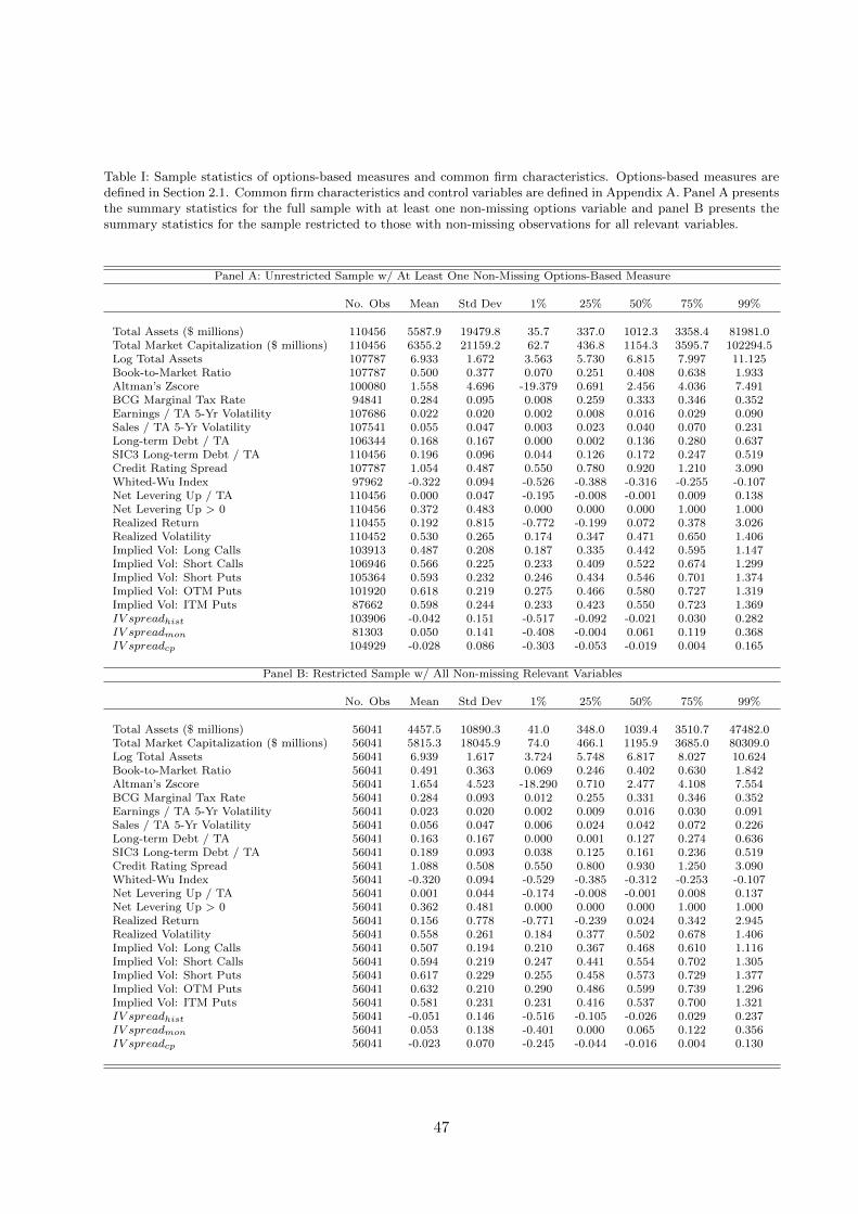
Table I: Sample statistics of options-based measures and common firm characteristics. Options-based measures aredefined in Section 2.1. Common firm characteristics and control variables are defined in Appendix A. Panel A presentsthe summary statistics for the full sample with at least one non-missing options variable and panel B presents thesummary statistics for the sample restricted to those with non-missing observations for all relevant variables.

Panel A: Unrestricted Sample w/ At Least One Non-Missing Options-Based Measure

No. Obs Mean Std Dev 1% 25% 50% 75% 99%

Total Assets ($ millions) 110456 5587.9 19479.8 35.7 337.0 1012.3 3358.4 81981.0Total Market Capitalization ($ millions) 110456 6355.2 21159.2 62.7 436.8 1154.3 3595.7 102294.5Log Total Assets 107787 6.933 1.672 3.563 5.730 6.815 7.997 11.125Book-to-Market Ratio 107787 0.500 0.377 0.070 0.251 0.408 0.638 1.933Altman’s Zscore 100080 1.558 4.696 -19.379 0.691 2.456 4.036 7.491BCG Marginal Tax Rate 94841 0.284 0.095 0.008 0.259 0.333 0.346 0.352Earnings / TA 5-Yr Volatility 107686 0.022 0.020 0.002 0.008 0.016 0.029 0.090Sales / TA 5-Yr Volatility 107541 0.055 0.047 0.003 0.023 0.040 0.070 0.231Long-term Debt / TA 106344 0.168 0.167 0.000 0.002 0.136 0.280 0.637SIC3 Long-term Debt / TA 110456 0.196 0.096 0.044 0.126 0.172 0.247 0.519Credit Rating Spread 107787 1.054 0.487 0.550 0.780 0.920 1.210 3.090Whited-Wu Index 97962 -0.322 0.094 -0.526 -0.388 -0.316 -0.255 -0.107Net Levering Up / TA 110456 0.000 0.047 -0.195 -0.008 -0.001 0.009 0.138Net Levering Up > 0 110456 0.372 0.483 0.000 0.000 0.000 1.000 1.000Realized Return 110455 0.192 0.815 -0.772 -0.199 0.072 0.378 3.026Realized Volatility 110452 0.530 0.265 0.174 0.347 0.471 0.650 1.406Implied Vol: Long Calls 103913 0.487 0.208 0.187 0.335 0.442 0.595 1.147Implied Vol: Short Calls 106946 0.566 0.225 0.233 0.409 0.522 0.674 1.299Implied Vol: Short Puts 105364 0.593 0.232 0.246 0.434 0.546 0.701 1.374Implied Vol: OTM Puts 101920 0.618 0.219 0.275 0.466 0.580 0.727 1.319Implied Vol: ITM Puts 87662 0.598 0.244 0.233 0.423 0.550 0.723 1.369IV spreadhist 103906 -0.042 0.151 -0.517 -0.092 -0.021 0.030 0.282IV spreadmon 81303 0.050 0.141 -0.408 -0.004 0.061 0.119 0.368IV spreadcp 104929 -0.028 0.086 -0.303 -0.053 -0.019 0.004 0.165

Panel B: Restricted Sample w/ All Non-missing Relevant Variables

No. Obs Mean Std Dev 1% 25% 50% 75% 99%

Total Assets ($ millions) 56041 4457.5 10890.3 41.0 348.0 1039.4 3510.7 47482.0Total Market Capitalization ($ millions) 56041 5815.3 18045.9 74.0 466.1 1195.9 3685.0 80309.0Log Total Assets 56041 6.939 1.617 3.724 5.748 6.817 8.027 10.624Book-to-Market Ratio 56041 0.491 0.363 0.069 0.246 0.402 0.630 1.842Altman’s Zscore 56041 1.654 4.523 -18.290 0.710 2.477 4.108 7.554BCG Marginal Tax Rate 56041 0.284 0.093 0.012 0.255 0.331 0.346 0.352Earnings / TA 5-Yr Volatility 56041 0.023 0.020 0.002 0.009 0.016 0.030 0.091Sales / TA 5-Yr Volatility 56041 0.056 0.047 0.006 0.024 0.042 0.072 0.226Long-term Debt / TA 56041 0.163 0.167 0.000 0.001 0.127 0.274 0.636SIC3 Long-term Debt / TA 56041 0.189 0.093 0.038 0.125 0.161 0.236 0.519Credit Rating Spread 56041 1.088 0.508 0.550 0.800 0.930 1.250 3.090Whited-Wu Index 56041 -0.320 0.094 -0.529 -0.385 -0.312 -0.253 -0.107Net Levering Up / TA 56041 0.001 0.044 -0.174 -0.008 -0.001 0.008 0.137Net Levering Up > 0 56041 0.362 0.481 0.000 0.000 0.000 1.000 1.000Realized Return 56041 0.156 0.778 -0.771 -0.239 0.024 0.342 2.945Realized Volatility 56041 0.558 0.261 0.184 0.377 0.502 0.678 1.406Implied Vol: Long Calls 56041 0.507 0.194 0.210 0.367 0.468 0.610 1.116Implied Vol: Short Calls 56041 0.594 0.219 0.247 0.441 0.554 0.702 1.305Implied Vol: Short Puts 56041 0.617 0.229 0.255 0.458 0.573 0.729 1.377Implied Vol: OTM Puts 56041 0.632 0.210 0.290 0.486 0.599 0.739 1.296Implied Vol: ITM Puts 56041 0.581 0.231 0.231 0.416 0.537 0.700 1.321IV spreadhist 56041 -0.051 0.146 -0.516 -0.105 -0.026 0.029 0.237IV spreadmon 56041 0.053 0.138 -0.401 0.000 0.065 0.122 0.356IV spreadcp 56041 -0.023 0.070 -0.245 -0.044 -0.016 0.004 0.130

47

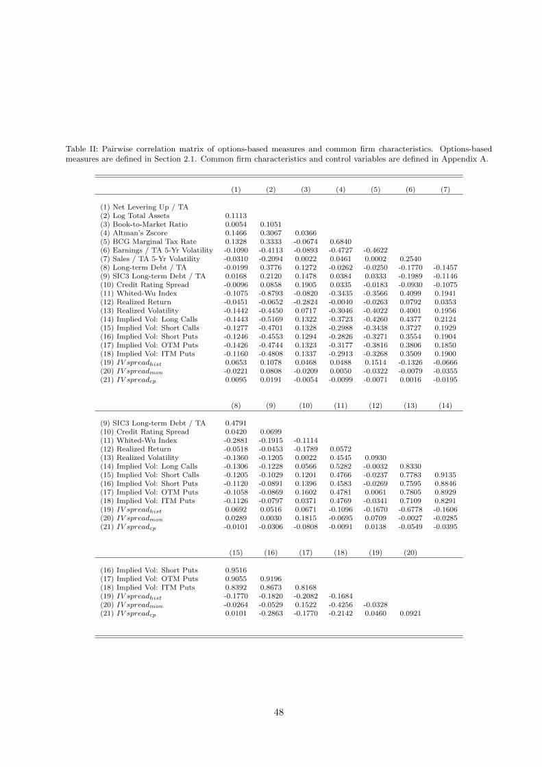
Table II: Pairwise correlation matrix of options-based measures and common firm characteristics. Options-basedmeasures are defined in Section 2.1. Common firm characteristics and control variables are defined in Appendix A.

(1) (2) (3) (4) (5) (6) (7)

(1) Net Levering Up / TA(2) Log Total Assets 0.1113(3) Book-to-Market Ratio 0.0054 0.1051(4) Altman’s Zscore 0.1466 0.3067 0.0366(5) BCG Marginal Tax Rate 0.1328 0.3333 -0.0674 0.6840(6) Earnings / TA 5-Yr Volatility -0.1090 -0.4113 -0.0893 -0.4727 -0.4622(7) Sales / TA 5-Yr Volatility -0.0310 -0.2094 0.0022 0.0461 0.0002 0.2540(8) Long-term Debt / TA -0.0199 0.3776 0.1272 -0.0262 -0.0250 -0.1770 -0.1457(9) SIC3 Long-term Debt / TA 0.0168 0.2120 0.1478 0.0384 0.0333 -0.1989 -0.1146(10) Credit Rating Spread -0.0096 0.0858 0.1905 0.0335 -0.0183 -0.0930 -0.1075(11) Whited-Wu Index -0.1075 -0.8793 -0.0820 -0.3435 -0.3566 0.4099 0.1941(12) Realized Return -0.0451 -0.0652 -0.2824 -0.0040 -0.0263 0.0792 0.0353(13) Realized Volatility -0.1442 -0.4450 0.0717 -0.3046 -0.4022 0.4001 0.1956(14) Implied Vol: Long Calls -0.1443 -0.5169 0.1322 -0.3723 -0.4260 0.4377 0.2124(15) Implied Vol: Short Calls -0.1277 -0.4701 0.1328 -0.2988 -0.3438 0.3727 0.1929(16) Implied Vol: Short Puts -0.1246 -0.4553 0.1294 -0.2826 -0.3271 0.3554 0.1904(17) Implied Vol: OTM Puts -0.1426 -0.4744 0.1323 -0.3177 -0.3816 0.3806 0.1850(18) Implied Vol: ITM Puts -0.1160 -0.4808 0.1337 -0.2913 -0.3268 0.3509 0.1900(19) IV spreadhist 0.0653 0.1078 0.0468 0.0488 0.1514 -0.1326 -0.0666(20) IV spreadmon -0.0221 0.0808 -0.0209 0.0050 -0.0322 -0.0079 -0.0355(21) IV spreadcp 0.0095 0.0191 -0.0054 -0.0099 -0.0071 0.0016 -0.0195

(8) (9) (10) (11) (12) (13) (14)

(9) SIC3 Long-term Debt / TA 0.4791(10) Credit Rating Spread 0.0420 0.0699(11) Whited-Wu Index -0.2881 -0.1915 -0.1114(12) Realized Return -0.0518 -0.0453 -0.1789 0.0572(13) Realized Volatility -0.1360 -0.1205 0.0022 0.4545 0.0930(14) Implied Vol: Long Calls -0.1306 -0.1228 0.0566 0.5282 -0.0032 0.8330(15) Implied Vol: Short Calls -0.1205 -0.1029 0.1201 0.4766 -0.0237 0.7783 0.9135(16) Implied Vol: Short Puts -0.1120 -0.0891 0.1396 0.4583 -0.0269 0.7595 0.8846(17) Implied Vol: OTM Puts -0.1058 -0.0869 0.1602 0.4781 0.0061 0.7805 0.8929(18) Implied Vol: ITM Puts -0.1126 -0.0797 0.0371 0.4769 -0.0341 0.7109 0.8291(19) IV spreadhist 0.0692 0.0516 0.0671 -0.1096 -0.1670 -0.6778 -0.1606(20) IV spreadmon 0.0289 0.0030 0.1815 -0.0695 0.0709 -0.0027 -0.0285(21) IV spreadcp -0.0101 -0.0306 -0.0808 -0.0091 0.0138 -0.0549 -0.0395

(15) (16) (17) (18) (19) (20)

(16) Implied Vol: Short Puts 0.9516(17) Implied Vol: OTM Puts 0.9055 0.9196(18) Implied Vol: ITM Puts 0.8392 0.8673 0.8168(19) IV spreadhist -0.1770 -0.1820 -0.2082 -0.1684(20) IV spreadmon -0.0264 -0.0529 0.1522 -0.4256 -0.0328(21) IV spreadcp 0.0101 -0.2863 -0.1770 -0.2142 0.0460 0.0921

48

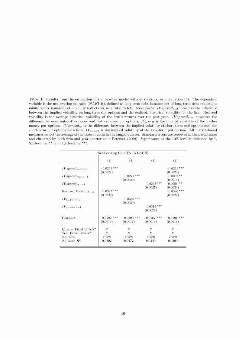
Table III: Results from the estimation of the baseline model without controls, as in equation (5). The dependentvariable is the net levering up ratio (NLEV R), defined as long-term debt issuance net of long-term debt reductionsminus equity issuance net of equity reductions, as a ratio to total book assets. IV spreadhist measures the differencebetween the implied volatility on long-term call options and the realized, historical volatility for the firm. Realizedvolatility is the average historical volatility of the firm’s returns over the past year. IV spreadmon measures thedifference between out-of-the-money and in-the-money put options. IVp,ITM is the implied volatility of the in-the-money put options. IV spreadcp is the difference between the implied volatility of short-term call options and theshort-term put options for a firm. IVp,short is the implied volatility of the long-term put options. All market-basedmeasures reflect the average of the three months in the lagged quarter. Standard errors are reported in the parenthesesand clustered by both firm and year-quarter as in Petersen (2009). Significance at the 10% level is indicated by *,5% level by **, and 1% level by ***.

Net Levering Up / TA (NLEV R)

(1) (2) (3) (4)

IV spreadhist,t−1 -0.0261 *** -0.0261 ***(0.0024) (0.0024)

IV spreadmon,t−1 -0.0271 *** -0.0032 **(0.0020) (0.0015)

IV spreadcp,t−1 -0.0203 *** 0.0056 **(0.0027) (0.0024)

Realized Volatilityt−1 -0.0387 *** -0.0386 ***(0.0022) (0.0022)

IVp,ITM,t−1 -0.0350 ***(0.0020)

IVp,short,t−1 -0.0319 ***(0.0022)

Constant 0.0192 *** 0.0200 *** 0.0187 *** 0.0191 ***(0.0016) (0.0016) (0.0016) (0.0016)

Quarter Fixed Effects? Y Y Y YYear Fixed Effects? Y Y Y YNo. Obs. 77389 77389 77389 77389Adjusted R2 0.0302 0.0272 0.0240 0.0303

49

Table IV: Results from the estimation of the full model with controls, as in equation (6). The dependent variable isthe net levering up ratio (NLEV R), defined as long-term debt issuance net of long-term debt reductions minus equityissuance net of equity reductions, as a ratio to total book assets. IV spreadhist measures the difference between theimplied volatility on long-term call options and the realized, historical volatility for the firm. IV spreadmon measuresthe difference between out-of-the-money and in-the-money put options. IV spreadcp is the difference between theimplied volatility of short-term call options and the short-term put options for a firm. Realized volatility is theaverage historical volatility of the firm’s returns over the past year. All market-based measures reflect the averageof the three months in the lagged quarter. All controls are defined in Appendix A. Standard errors are reported inthe parentheses and clustered by both firm and year-quarter as in Petersen (2009). Significance at the 10% level isindicated by *, 5% level by **, and 1% level by ***.

Net Levering Up / TA (NLEV R)

(1) (2) (3) (4) (5)

IV spreadhist,t−1 -0.0103 *** -0.0100 ***(0.0027) (0.0027)

IV spreadmon,t−1 -0.0048 *** -0.0047 ***(0.0014) (0.0014)

IV spreadcp,t−1 0.0028 0.0041 *(0.0023) (0.0023)

Realized Volatilityt−1 -0.0180 *** -0.0124 *** -0.0125 *** -0.0177 ***(0.0025) (0.0018) (0.0019) (0.0025)

Realized Returnt−1 -0.0026 *** -0.0022 *** -0.0021 *** -0.0022 *** -0.0022 ***(0.0004) (0.0004) (0.0004) (0.0004) (0.0004)

Log Total Assetst−1 0.0021 *** 0.0017 *** 0.0019 *** 0.0018 *** 0.0017 ***(0.0004) (0.0004) (0.0004) (0.0004) (0.0004)

Book-to-Market Ratiot−1 -0.0008 0.0005 0.0000 0.0001 0.0004(0.0008) (0.0008) (0.0008) (0.0008) (0.0008)

Altman’s Zscoret−1 0.0010 *** 0.0009 *** 0.0009 *** 0.0009 *** 0.0009 ***(0.0001) (0.0001) (0.0001) (0.0001) (0.0001)

BCG Marginal Tax Ratet−1 0.0082 ** 0.0008 0.0018 0.0018 0.0008(0.0040) (0.0040) (0.0040) (0.0040) (0.0040)

Earnings / TA 5-Yr Volatilityt−1 -0.0401 ** -0.0122 -0.0175 -0.0181 -0.0121(0.0186) (0.0177) (0.0180) (0.0181) (0.0176)

Sales / TA 5-Yr Volatilityt−1 -0.0162 *** -0.0116 * -0.0125 ** -0.0125 ** -0.0114 *(0.0060) (0.0062) (0.0061) (0.0061) (0.0061)

Long-term Debt / TAt−1 -0.0171 *** -0.0167 *** -0.0169 *** -0.0170 *** -0.0166 ***(0.0022) (0.0022) (0.0022) (0.0022) (0.0022)

SIC3 Long-term Debt / TAt−1 0.0092 *** 0.0067 ** 0.0072 ** 0.0073 ** 0.0067 **(0.0032) (0.0031) (0.0031) (0.0031) (0.0031)

Credit Rating Spreadt−1 -0.0015 -0.0011 -0.0018 * -0.0018 * -0.0010(0.0012) (0.0011) (0.0010) (0.0010) (0.0011)

Whited-Wu Indext−1 -0.0032 0.0038 0.0027 0.0022 0.0039(0.0062) (0.0062) (0.0061) (0.0061) (0.0062)

Constant -0.0121 *** 0.0033 -0.0010 -0.0005 0.0027(0.0025) (0.0034) (0.0031) (0.0031) (0.0034)

Quarter Fixed Effects? Y Y Y Y YYear Fixed Effects? Y Y Y Y YNo. Obs. 56041 56041 56041 56041 56041Adjusted R2 0.0389 0.0417 0.0415 0.0413 0.0419

50

Table V: Results from the estimation of the modified full model with first lagged differences and second laggedlevels, as in equation (7). The dependent variable is the net levering up ratio (NLEV R), defined as long-term debtissuance net of long-term debt reductions minus equity issuance net of equity reductions, as a ratio to total bookassets. IV spreadhist measures the difference between the implied volatility on long-term call options and the realized,historical volatility for the firm. IV spreadmon measures the difference between out-of-the-money and in-the-moneyput options. IV spreadcp is the difference between the implied volatility of short-term call options and the short-termput options for a firm. Realized volatility is the average historical volatility of the firm’s returns over the past year.All market-based measures reflect the average of the three months in the lagged quarter. All controls are definedin Appendix A. Standard errors are reported in the parentheses and clustered by both firm and year-quarter as inPetersen (2009). Significance at the 10% level is indicated by *, 5% level by **, and 1% level by ***.

Net Levering Up / TA (NLEV R)

(1) (2) (3) (4) (5)

∆IV spreadhist,t−2,t−1 -0.0099 *** -0.0097 **(0.0038) (0.0038)

∆IV spreadmon,t−2,t−1 -0.0043 ** -0.0038 **(0.0019) (0.0019)

∆IV spreadcp,t−2,t−1 0.0015 0.0029(0.0027) (0.0026)

∆Realized Volatilityt−2,t−1 -0.0112 * -0.0124 ** -0.0124 ** -0.0111 *(0.0062) (0.0053) (0.0053) (0.0062)

∆Realized Returnt−2,t−1 -0.0037 *** -0.0037 *** -0.0032 *** -0.0033 *** -0.0036 ***(0.0007) (0.0008) (0.0008) (0.0008) (0.0008)

∆Log Total Assetst−2,t−1 -0.0110 *** -0.0109 *** -0.0107 *** -0.0109 *** -0.0107 ***(0.0034) (0.0034) (0.0034) (0.0034) (0.0034)

∆Book-to-Market Ratiot−2,t−1 0.0038 ** 0.0046 *** 0.0040 *** 0.0041 *** 0.0045 ***(0.0016) (0.0016) (0.0015) (0.0015) (0.0016)

∆Altman’s Zscoret−2,t−1 0.0011 *** 0.0010 *** 0.0011 *** 0.0011 *** 0.0010 ***(0.0002) (0.0002) (0.0002) (0.0002) (0.0002)

∆BCG Marginal Tax Ratet−2,t−1 -0.0054 -0.0107 -0.0091 -0.0090 -0.0108(0.0090) (0.0095) (0.0094) (0.0094) (0.0095)

∆Earnings / TA 5-Yr Volatilityt−2,t−1 -0.0710 -0.0412 -0.0492 -0.0480 -0.0422

(0.0570) (0.0559) (0.0567) (0.0567) (0.0560)∆Sales / TA 5-Yr Volatilityt−2,t−1 -0.0628 ** -0.0556 * -0.0562 * -0.0560 * -0.0559 *

(0.0310) (0.0312) (0.0311) (0.0311) (0.0311)∆Long-term Debt / TAt−2,t−1 0.0200 *** 0.0200 *** 0.0194 *** 0.0196 *** 0.0199 ***

(0.0074) (0.0073) (0.0073) (0.0073) (0.0073)∆SIC3 Long-term Debt / TAt−2,t−1 0.0183 0.0163 0.0166 0.0169 0.0161

(0.0113) (0.0116) (0.0116) (0.0116) (0.0116)∆Credit Rating Spreadt−2,t−1 -0.0019 ** -0.0018 ** -0.0024 *** -0.0023 *** -0.0018 **

(0.0010) (0.0009) (0.0008) (0.0008) (0.0009)∆Whited-Wu Indext−2,t−1 0.0057 0.0119 * 0.0102 * 0.0098 0.0121 *

(0.0062) (0.0063) (0.0062) (0.0062) (0.0063)

Continued below.

51

Continued from above.

(1) (2) (3) (4) (5)

IV spreadhist,t−2 -0.0172 *** -0.0168 ***(0.0035) (0.0035)

IV spreadmon,t−2 -0.0060 *** -0.0054 **(0.0023) (0.0023)

IV spreadcp,t−2 0.0008 0.0037(0.0033) (0.0033)

Realized Volatilityt−2 -0.0194 *** -0.0104 *** -0.0105 *** -0.0190 ***(0.0027) (0.0018) (0.0018) (0.0028)

Realized Returnt−2 -0.0026 *** -0.0022 *** -0.0020 *** -0.0021 *** -0.0021 ***(0.0004) (0.0004) (0.0004) (0.0004) (0.0004)

Log Total Assetst−2 0.0024 *** 0.0022 *** 0.0024 *** 0.0023 *** 0.0022 ***(0.0005) (0.0005) (0.0005) (0.0005) (0.0005)

Book-to-Market Ratiot−2 -0.0030 *** -0.0015 * -0.0022 *** -0.0022 ** -0.0017 *(0.0009) (0.0009) (0.0009) (0.0009) (0.0009)

Altman’s Zscoret−2 0.0009 *** 0.0009 *** 0.0009 *** 0.0009 *** 0.0009 ***(0.0001) (0.0001) (0.0001) (0.0001) (0.0001)

BCG Marginal Tax Ratet−2 0.0085 * 0.0021 0.0039 0.0040 0.0021(0.0045) (0.0045) (0.0046) (0.0046) (0.0045)

Earnings / TA 5-Yr Volatilityt−2 -0.0396 * -0.0128 -0.0211 -0.0216 -0.0126(0.0205) (0.0196) (0.0200) (0.0201) (0.0196)

Sales / TA 5-Yr Volatilityt−2 -0.0116 * -0.0069 -0.0084 -0.0085 -0.0067(0.0067) (0.0067) (0.0067) (0.0067) (0.0067)

Long-term Debt / TAt−2 -0.0209 *** -0.0204 *** -0.0206 *** -0.0207 *** -0.0203 ***(0.0025) (0.0025) (0.0025) (0.0025) (0.0025)

SIC3 Long-term Debt / TAt−2 0.0099 *** 0.0077 ** 0.0084 ** 0.0084 ** 0.0077 **(0.0037) (0.0036) (0.0036) (0.0036) (0.0036)

Credit Rating Spreadt−2 -0.0045 *** -0.0035 *** -0.0041 *** -0.0043 *** -0.0033 ***(0.0012) (0.0013) (0.0012) (0.0012) (0.0013)

Whited-Wu Indext−2 -0.0028 0.0100 0.0063 0.0056 0.0102(0.0081) (0.0080) (0.0079) (0.0080) (0.0080)

Constant -0.0100 *** 0.0054 -0.0013 -0.0006 0.0046(0.0032) (0.0040) (0.0036) (0.0036) (0.0040)

Quarter Fixed Effects? Y Y Y Y YYear Fixed Effects? Y Y Y Y YNo. Obs. 44105 44105 44105 44105 44105Adjusted R2 0.0408 0.0432 0.0426 0.0424 0.0433

52

Table VI: Results from the estimation of the full model, as in equation (6), using unconditional sub-samples of varyingsupply and demand for financing. Columns (1) and (2) sub-sample all observations into boom and bust years. Weuse two events to define boom and bust years: the dot-com bubble and the financial crisis. Boom periods are definedto be 1996Q1 through 1999Q4 and 2005Q1 through 2007Q2. Bust periods are defined to be 2001Q1 through 2002Q4and 2007Q3 through 2009Q2. Colunns (3) and (4) sub-sample all firms into three equal-sized bins based on the book-to-market ratio each quarter with Low BTM defined as the bottom tercile and High BTM defined as the top tercile.The dependent variable is the net levering up ratio (NLEV R), defined as long-term debt issuance net of long-termdebt reductions minus equity issuance net of equity reductions, as a ratio to total book assets. IV spreadhist measuresthe difference between the implied volatility on long-term call options and the realized, historical volatility for thefirm. IV spreadmon measures the difference between out of the money and at the money put options. IV spreadcpis the difference between the implied volatility of long-term call options and the long-term put options for a firm.Realized volatility is the average historical volatility of the firm’s returns over the past year. All explanatory variablesare lagged at one quarter. All market-based measures reflect the average of the three months in the past quarter. Allcontrols are defined in Appendix A. Standard errors are reported in the parentheses and clustered by both firm andyear-quarter as in Petersen (2009). Significance at the 10% level is indicated by *, 5% level by **, and 1% level by***.

Net Levering Up / TA (NLEV R)

Boom Years Bust Years Low BTM High BTM(1) (2) (3) (4)

IV spreadhist,t−1 -0.0149 *** -0.0097 ** -0.0122 ** -0.0069 *(0.0042) (0.0044) (0.0048) (0.0037)

IV spreadmon,t−1 -0.0057 ** -0.0064 ** -0.0112 *** -0.0003(0.0025) (0.0028) (0.0030) (0.0017)

IV spreadcp,t−1 0.0056 0.0019 0.0159 ** -0.0048 *(0.0042) (0.0038) (0.0073) (0.0026)

Realized Volatilityt−1 -0.0226 *** -0.0146 *** -0.0194 *** -0.0141 ***(0.0039) (0.0036) (0.0035) (0.0028)

Realized Returnt−1 -0.0040 *** -0.0020 *** -0.0013 *** -0.0015 **(0.0007) (0.0005) (0.0005) (0.0007)

Log Total Assetst−1 0.0007 0.0025 *** 0.0020 *** 0.0009 *(0.0007) (0.0006) (0.0007) (0.0005)

Book-to-Market Ratiot−1 0.0008 -0.0008 0.0184 *** -0.0012(0.0016) (0.0011) (0.0049) (0.0009)

Altman’s Zscoret−1 0.0010 *** 0.0010 *** 0.0011 *** 0.0002(0.0001) (0.0002) (0.0002) (0.0001)

BCG Marginal Tax Ratet−1 0.0107 -0.0069 0.0011 0.0045(0.0071) (0.0075) (0.0076) (0.0053)

Earnings / TA 5-Yr Volatilityt−1 -0.0156 -0.0026 -0.0052 0.0093(0.0274) (0.0280) (0.0288) (0.0208)

Sales / TA 5-Yr Volatilityt−1 -0.0148 * -0.0092 -0.0023 -0.0176 **(0.0079) (0.0090) (0.0117) (0.0079)

Long-term Debt / TAt−1 -0.0113 *** -0.0246 *** -0.0070 ** -0.0190 ***(0.0041) (0.0035) (0.0035) (0.0029)

SIC3 Long-term Debt / TAt−1 0.0175 *** 0.0080 * -0.0032 0.0114 ***(0.0053) (0.0042) (0.0052) (0.0042)

Credit Rating Spreadt−1 0.0016 -0.0040 *** 0.0000 -0.0006(0.0042) (0.0010) (0.0015) (0.0009)

Whited-Wu Indext−1 -0.0017 0.0059 -0.0071 0.0066(0.0100) (0.0089) (0.0108) (0.0087)

Constant 0.0025 0.0046 -0.0066 0.0080 *(0.0068) (0.0056) (0.0049) (0.0044)

Quarter Fixed Effects? Y Y Y YYear Fixed Effects? Y Y Y YNo. Obs. 17771 18444 18871 18186Adjusted R2 0.0393 0.0470 0.0668 0.0229

53

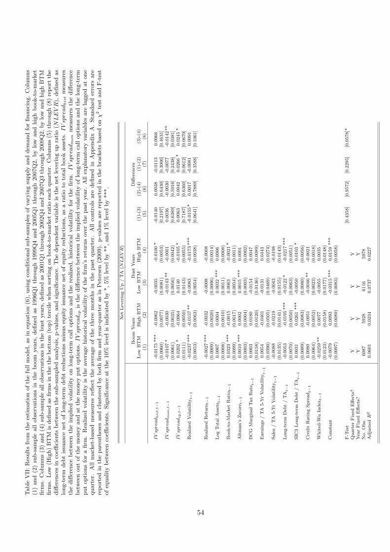
Table

VII

:R

esult

sfr

om

the

esti

mati

on

of

the

full

model

,as

ineq

uati

on

(6),

usi

ng

condit

ional

sub-s

am

ple

sof

vary

ing

supply

and

dem

and

for

financi

ng.

Colu

mns

(1)

and

(2)

sub-s

am

ple

all

obse

rvati

ons

inth

eb

oom

yea

rs,

defi

ned

as

1996Q

1th

rough

1999Q

4and

2005Q

1th

rough

2007Q

2,

by

low

and

hig

hb

ook-t

o-m

ark

etfirm

s.C

olu

mns

(3)

and

(4)

sub-s

am

ple

all

obse

rvati

ons

inth

ebust

yea

rs,

defi

ned

as

2001Q

1th

rough

2002Q

4and

2007Q

3th

rough

2009Q

2,

by

low

and

hig

hB

TM

firm

s.L

ow(H

igh)

BT

Mis

defi

ned

as

firm

sin

the

the

bott

om

(top)

terc

ile

when

sort

ing

on

book-t

o-m

ark

etra

tio

each

quart

er.

Colu

mns

(5)

thro

ugh

(8)

rep

ort

the

diff

eren

ces

inco

effici

ents

bet

wee

nth

esu

b-s

am

ple

danaly

sis,

p-v

alu

es,

and

signifi

cance

.T

he

dep

enden

tva

riable

isth

enet

lever

ing

up

rati

o(NLEVR

),defi

ned

as

long-t

erm

deb

tis

suance

net

of

long-t

erm

deb

tre

duct

ions

min

us

equit

yis

suance

net

of

equit

yre

duct

ions,

as

ara

tio

toto

tal

book

ass

ets.IVspreadhis

tm

easu

res

the

diff

eren

ceb

etw

een

the

implied

vola

tility

on

long-t

erm

call

opti

ons

and

the

realize

d,

his

tori

cal

vola

tility

for

the

firm

.IVspreadm

on

mea

sure

sth

ediff

eren

ceb

etw

een

out

of

the

money

and

at

the

money

put

opti

ons.IVspreadcp

isth

ediff

eren

ceb

etw

een

the

implied

vola

tility

of

long-t

erm

call

opti

ons

and

the

long-t

erm

put

opti

ons

for

afirm

.R

ealize

dvola

tility

isth

eav

erage

his

tori

cal

vola

tility

of

the

firm

’sre

turn

sov

erth

epast

yea

r.A

llex

pla

nato

ryva

riable

sare

lagged

at

one

quart

er.

All

mark

et-b

ase

dm

easu

res

reflec

tth

eav

erage

of

the

thre

em

onth

sin

the

past

quart

er.

All

contr

ols

are

defi

ned

inA

pp

endix

A.

Sta

ndard

erro

rsare

rep

ort

edin

the

pare

nth

eses

and

clust

ered

by

both

firm

and

yea

r-quart

eras

inP

eter

sen

(2009).

p-v

alu

esare

rep

ort

edin

the

bra

cket

sbase

donχ2

test

and

F-t

est

of

equality

bet

wee

nco

effici

ents

.Sig

nifi

cance

at

the

10%

level

isin

dic

ate

dby

*,

5%

level

by

**,

and

1%

level

by

***.

Net

Lev

erin

gU

p/

TA

(NLEVR

)

Boom

Yea

rsB

ust

Yea

rsD

iffer

ence

sL

ow

BT

MH

igh

BT

ML

ow

BT

MH

igh

BT

M(1

)-(3

)(2

)-(4

)(1

)-(2

)(3

)-(4

)(1

)(2

)(3

)(4

)(5

)(6

)(7

)(8

)

IVsp

rea

dhis

t,t−

1-0

.0175

***

-0.0

062

-0.0

035

-0.0

100

*-0

.0140

0.0

038

-0.0

113

0.0

066

(0.0

060)

(0.0

077)

(0.0

081)

(0.0

053)

[0.2

197]

[0.6

430]

[0.3

006]

[0.4

631]

IVsp

rea

dm

on,t−1

-0.0

107

*-0

.0030

-0.0

143

**

-0.0

001

0.0

036

-0.0

030

-0.0

077

-0.0

142

**

(0.0

061)

(0.0

035)

(0.0

056)

(0.0

042)

[0.6

389]

[0.5

916]

[0.2

438]

[0.0

381]

IVsp

rea

dcp,t−1

0.0

202

*-0

.0064

0.0

140

-0.0

105

*0.0

063

0.0

042

0.0

266

*0.0

245

*(0

.0111)

(0.0

050)

(0.0

143)

(0.0

055)

[0.7

187]

[0.6

360]

[0.0

612]

[0.0

670]

Rea

lize

dV

ola

tility

t−1

-0.0

237

***

-0.0

157

**

-0.0

083

-0.0

173

***

-0.0

155

*0.0

017

-0.0

081

0.0

091

(0.0

053)

(0.0

063)

(0.0

054)

(0.0

038)

[0.0

641]

[0.7

889]

[0.3

588]

[0.1

061]

Rea

lize

dR

etu

rnt−

1-0

.0027

***

-0.0

032

-0.0

008

-0.0

008

(0.0

009)

(0.0

020)

(0.0

006)

(0.0

014)

Log

Tota

lA

sset

s t−1

0.0

007

0.0

004

0.0

032

***

0.0

006

(0.0

008)

(0.0

010)

(0.0

011)

(0.0

008)

Book-t

o-M

ark

etR

ati

ot−

10.0

323

***

-0.0

015

0.0

063

-0.0

021

*(0

.0099)

(0.0

017)

(0.0

054)

(0.0

011)

Alt

man

’sZ

score

t−1

0.0

010

***

0.0

002

0.0

015

***

0.0

001

(0.0

003)

(0.0

004)

(0.0

003)

(0.0

002)

BC

GM

arg

inal

Tax

Rate

t−1

0.0

003

0.0

180

-0.0

154

0.0

047

(0.0

158)

(0.0

120)

(0.0

136)

(0.0

089)

Earn

ings

/T

A5-Y

rV

ola

tility

t−1

0.0

054

-0.0

401

-0.0

131

0.0

443

(0.0

390)

(0.0

505)

(0.0

469)

(0.0

274)

Sale

s/

TA

5-Y

rV

ola

tility

t−1

-0.0

088

-0.0

219

-0.0

043

-0.0

198

(0.0

135)

(0.0

141)

(0.0

155)

(0.0

143)

Lon

g-t

erm

Deb

t/

TA

t−1

-0.0

053

-0.0

195

***

-0.0

122

*-0

.0217

***

(0.0

070)

(0.0

050)

(0.0

063)

(0.0

051)

SIC

3L

on

g-t

erm

Deb

t/

TA

t−1

0.0

031

0.0

261

***

-0.0

050

0.0

103

*(0

.0089)

(0.0

083)

(0.0

080)

(0.0

056)

Cre

dit

Rati

ng

Sp

readt−

10.0

080

-0.0

051

-0.0

046

**

-0.0

021

(0.0

064)

(0.0

052)

(0.0

023)

(0.0

018)

Wh

ited

-Wu

Ind

ext−

1-0

.0259

**

0.0

077

-0.0

055

0.0

035

(0.0

123)

(0.0

158)

(0.0

177)

(0.0

148)

Con

stant

-0.0

079

0.0

093

-0.0

315

***

0.0

159

***

(0.0

097)

(0.0

089)

(0.0

083)

(0.0

058)

F-T

est

[0.4

358]

[0.9

572]

[0.2

295]

[0.0

578]*

Qu

art

erF

ixed

Eff

ects

?Y

YY

YY

ear

Fix

edE

ffec

ts?

YY

YY

No.

Ob

s.6087

5928

6116

5978

Ad

just

edR

20.0

601

0.0

234

0.0

737

0.0

227

54

Table VIII: Results from the estimation of equation (6) using option counts in place of the options-based risk measures.The dependent variable is the net levering up ratio (NLEV R), defined as long-term debt issuance net of long-termdebt reductions minus equity issuance net of equity reductions, as a ratio to total book assets. Has Tradeable Optionsis a dummy variable that equals 1 if the firm has tradeable options in the market over the three months in the pastquarter and 0 otherwise. Log Total Tradeable Options is the natural log of the total number of tradeable options afirm has in the market over a month averaged over the three months in the past quarter. Log Total Open Interestis the natural log of the open interest a firm has in the market over a month averaged over the three months in thepast quarter. Log Total Volume is the natural log of the total number of options traded in the market for the firmover a month averaged over the three months in the past quarter. All explanatory variables are lagged one quarter.All controls are defined in Appendix A. Standard errors are reported in the parentheses and clustered by both firmand year-quarter as in Petersen (2009). Significance at the 10% level is indicated by *, 5% level by **, and 1% levelby ***.

Net Levering Up / TA (NLEV R)

(1) (2) (3) (4)

Has Tradeable Optionst−1 0.0004(0.0004)

Log Total Tradeable Optionst−1 0.0004 ***(0.0002)

Log Total Open Interestt−1 0.0001 **(0.0001)

Log Total Volumet−1 0.0002 ***(0.0001)

Realized Volatilityt−1 -0.0038 *** -0.0041 *** -0.0040 *** -0.0042 ***(0.0008) (0.0008) (0.0008) (0.0008)

Realized Returnt−1 -0.0032 *** -0.0032 *** -0.0032 *** -0.0032 ***(0.0003) (0.0003) (0.0003) (0.0003)

Log Total Assetst−1 0.0014 *** 0.0011 *** 0.0012 *** 0.0011 ***(0.0002) (0.0002) (0.0002) (0.0002)

Book-to-Market Ratiot−1 0.0014 *** 0.0017 *** 0.0016 *** 0.0016 ***(0.0004) (0.0004) (0.0004) (0.0004)

Altman’s Zscoret−1 0.0007 *** 0.0007 *** 0.0007 *** 0.0007 ***(0.0001) (0.0001) (0.0001) (0.0001)

BCG Marginal Tax Ratet−1 0.0053 ** 0.0050 ** 0.0052 ** 0.0052 **(0.0024) (0.0024) (0.0024) (0.0024)

Earnings / TA 5-Yr Volatilityt−1 -0.0489 *** -0.0512 *** -0.0511 *** -0.0514 ***(0.0109) (0.0109) (0.0109) (0.0109)

Sales / TA 5-Yr Volatilityt−1 -0.0055 -0.0053 -0.0054 -0.0055(0.0034) (0.0034) (0.0034) (0.0034)

Long-term Debt / TAt−1 -0.0153 *** -0.0149 *** -0.0150 *** -0.0149 ***(0.0018) (0.0018) (0.0018) (0.0018)

SIC3 Long-term Debt / TAt−1 0.0114 *** 0.0117 *** 0.0116 *** 0.0117 ***(0.0021) (0.0021) (0.0021) (0.0021)

Credit Rating Spreadt−1 -0.0008 -0.0008 -0.0008 -0.0008(0.0006) (0.0006) (0.0006) (0.0006)

Whited-Wu Indext−1 -0.0055 * -0.0062 * -0.0061 * -0.0062 *(0.0033) (0.0033) (0.0033) (0.0033)

Constant -0.0050 *** -0.0037 ** -0.0040 ** -1.2994 ***(0.0015) (0.0016) (0.0016) (0.0952)

Quarter Fixed Effects? Y Y Y YYear Fixed Effects? Y Y Y YNo. Obs. 183032 183032 183032 183032Adjusted R2 0.0332 0.0333 0.0333 0.0333

55

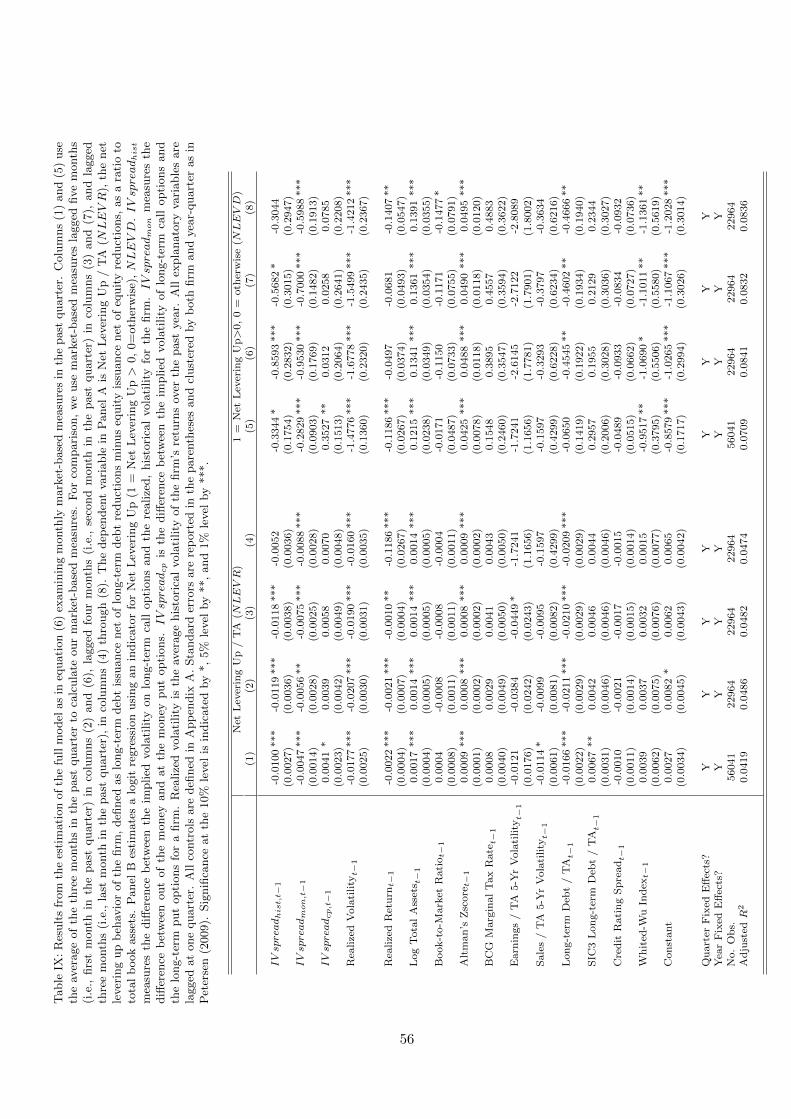
Table

IX:

Res

ult

sfr

om

the

esti

mati

on

of

the

full

model

as

ineq

uati

on

(6)

exam

inin

gm

onth

lym

ark

et-b

ase

dm

easu

res

inth

epast

quart

er.

Colu

mns

(1)

and

(5)

use

the

aver

age

of

the

thre

em

onth

sin

the

past

quart

erto

calc

ula

teour

mark

et-b

ase

dm

easu

res.

For

com

pari

son,

we

use

mark

et-b

ase

dm

easu

res

lagged

five

month

s(i

.e.,

firs

tm

onth

inth

epast

quart

er)

inco

lum

ns

(2)

and

(6),

lagged

four

month

s(i

.e.,

seco

nd

month

inth

epast

quart

er)

inco

lum

ns

(3)

and

(7),

and

lagged

thre

em

onth

s(i

.e.,

last

month

inth

epast

quart

er),

inco

lum

ns

(4)

thro

ugh

(8).

The

dep

enden

tva

riable

inP

anel

Ais

Net

Lev

erin

gU

p/

TA

(NLEVR

),th

enet

lever

ing

up

beh

avio

rof

the

firm

,defi

ned

as

long-t

erm

deb

tis

suance

net

of

long-t

erm

deb

tre

duct

ions

min

us

equit

yis

suance

net

of

equit

yre

duct

ions,

as

ara

tio

toto

tal

book

ass

ets.

Panel

Bes

tim

ate

sa

logit

regre

ssio

nusi

ng

an

indic

ato

rfo

rN

etL

ever

ing

Up

(1=

Net

Lev

erin

gU

p>

0,

0=

oth

erw

ise)

,NLEVD

.IVspreadhis

t

mea

sure

sth

ediff

eren

ceb

etw

een

the

implied

vola

tility

on

long-t

erm

call

opti

ons

and

the

realize

d,

his

tori

cal

vola

tility

for

the

firm

.IVspreadm

on

mea

sure

sth

ediff

eren

ceb

etw

een

out

of

the

money

and

at

the

money

put

opti

ons.

IVspreadcp

isth

ediff

eren

ceb

etw

een

the

implied

vola

tility

of

long-t

erm

call

opti

ons

and

the

long-t

erm

put

opti

ons

for

afirm

.R

ealize

dvola

tility

isth

eav

erage

his

tori

cal

vola

tility

of

the

firm

’sre

turn

sov

erth

epast

yea

r.A

llex

pla

nato

ryva

riable

sare

lagged

at

one

quart

er.

All

contr

ols

are

defi

ned

inA

pp

endix

A.

Sta

ndard

erro

rsare

rep

ort

edin

the

pare

nth

eses

and

clust

ered

by

both

firm

and

yea

r-quart

eras

inP

eter

sen

(2009).

Sig

nifi

cance

at

the

10%

level

isin

dic

ate

dby

*,

5%

level

by

**,

and

1%

level

by

***.

Net

Lev

erin

gU

p/

TA

(NLEVR

)1

=N

etL

ever

ing

Up>

0,

0=

oth

erw

ise

(NLEVD

)(1

)(2

)(3

)(4

)(5

)(6

)(7

)(8

)

IVsp

rea

dhis

t,t−

1-0

.0100

***

-0.0

119

***

-0.0

118

***

-0.0

052

-0.3

344

*-0

.8593

***

-0.5

682

*-0

.3044

(0.0

027)

(0.0

036)

(0.0

038)

(0.0

036)

(0.1

754)

(0.2

832)

(0.3

015)

(0.2

947)

IVsp

rea

dm

on,t−1

-0.0

047

***

-0.0

056

**

-0.0

075

***

-0.0

088

***

-0.2

829

***

-0.9

530

***

-0.7

000

***

-0.5

988

***

(0.0

014)

(0.0

028)

(0.0

025)

(0.0

028)

(0.0

903)

(0.1

769)

(0.1

482)

(0.1

913)

IVsp

rea

dcp,t−1

0.0

041

*0.0

039

0.0

058

0.0

070

0.3

527

**

0.0

312

0.0

258

0.0

785

(0.0

023)

(0.0

042)

(0.0

049)

(0.0

048)

(0.1

513)

(0.2

064)

(0.2

641)

(0.2

208)

Rea

lize

dV

ola

tility

t−1

-0.0

177

***

-0.0

207

***

-0.0

190

***

-0.0

160

***

-1.4

776

***

-1.6

778

***

-1.5

499

***

-1.4

212

***

(0.0

025)

(0.0

030)

(0.0

031)

(0.0

035)

(0.1

360)

(0.2

320)

(0.2

435)

(0.2

367)

Rea

lize

dR

etu

rnt−

1-0

.0022

***

-0.0

021

***

-0.0

010

**

-0.1

186

***

-0.1

186

***

-0.0

497

-0.0

681

-0.1

407

**

(0.0

004)

(0.0

007)

(0.0

004)

(0.0

267)

(0.0

267)

(0.0

374)

(0.0

493)

(0.0

547)

Log

Tota

lA

sset

s t−1

0.0

017

***

0.0

014

***

0.0

014

***

0.0

014

***

0.1

215

***

0.1

341

***

0.1

361

***

0.1

391

***

(0.0

004)

(0.0

005)

(0.0

005)

(0.0

005)

(0.0

238)

(0.0

349)

(0.0

354)

(0.0

355)

Book-t

o-M

ark

etR

ati

ot−

10.0

004

-0.0

008

-0.0

008

-0.0

004

-0.0

171

-0.1

150

-0.1

171

-0.1

477

*(0

.0008)

(0.0

011)

(0.0

011)

(0.0

011)

(0.0

487)

(0.0

733)

(0.0

755)

(0.0

791)

Alt

man

’sZ

score

t−1

0.0

009

***

0.0

008

***

0.0

008

***

0.0

009

***

0.0

425

***

0.0

488

***

0.0

490

***

0.0

495

***

(0.0

001)

(0.0

002)

(0.0

002)

(0.0

002)

(0.0

078)

(0.0

118)

(0.0

118)

(0.0

120)

BC

GM

arg

inal

Tax

Rate

t−1

0.0

008

0.0

029

0.0

041

0.0

043

0.1

548

0.3

895

0.4

557

0.4

883

(0.0

040)

(0.0

049)

(0.0

050)

(0.0

050)

(0.2

460)

(0.3

547)

(0.3

594)

(0.3

622)

Earn

ings

/T

A5-Y

rV

ola

tility

t−1

-0.0

121

-0.0

384

-0.0

449

*-1

.7241

-1.7

241

-2.6

145

-2.7

122

-2.8

089

(0.0

176)

(0.0

242)

(0.0

243)

(1.1

656)

(1.1

656)

(1.7

781)

(1.7

901)

(1.8

002)

Sale

s/

TA

5-Y

rV

ola

tility

t−1

-0.0

114

*-0

.0099

-0.0

095

-0.1

597

-0.1

597

-0.3

293

-0.3

797

-0.3

634

(0.0

061)

(0.0

081)

(0.0

082)

(0.4

299)

(0.4

299)

(0.6

228)

(0.6

234)

(0.6

216)

Lon

g-t

erm

Deb

t/

TA

t−1

-0.0

166

***

-0.0

211

***

-0.0

210

***

-0.0

209

***

-0.0

650

-0.4

545

**

-0.4

602

**

-0.4

666

**

(0.0

022)

(0.0

029)

(0.0

029)

(0.0

029)

(0.1

419)

(0.1

922)

(0.1

934)

(0.1

940)

SIC

3L

on

g-t

erm

Deb

t/

TA

t−1

0.0

067

**

0.0

042

0.0

046

0.0

044

0.2

957

0.1

955

0.2

129

0.2

344

(0.0

031)

(0.0

046)

(0.0

046)

(0.0

046)

(0.2

006)

(0.3

028)

(0.3

036)

(0.3

027)

Cre

dit

Rati

ng

Sp

readt−

1-0

.0010

-0.0

021

-0.0

017

-0.0

015

-0.0

489

-0.0

933

-0.0

834

-0.0

932

(0.0

011)

(0.0

014)

(0.0

015)

(0.0

014)

(0.0

515)

(0.0

662)

(0.0

727)

(0.0

736)

Wh

ited

-Wu

Ind

ext−

10.0

039

0.0

037

0.0

032

0.0

015

-0.9

517

**

-1.0

690

*-1

.1011

**

-1.1

361

**

(0.0

062)

(0.0

075)

(0.0

076)

(0.0

077)

(0.3

795)

(0.5

506)

(0.5

580)

(0.5

619)

Con

stant

0.0

027

0.0

082

*0.0

062

0.0

065

-0.8

579

***

-1.0

265

***

-1.1

067

***

-1.2

028

***

(0.0

034)

(0.0

045)

(0.0

043)

(0.0

042)

(0.1

717)

(0.2

994)

(0.3

026)

(0.3

014)

Qu

art

erF

ixed

Eff

ects

?Y

YY

YY

YY

YY

ear

Fix

edE

ffec

ts?

YY

YY

YY

YY

No.

Ob

s.56041

22964

22964

22964

56041

22964

22964

22964

Ad

just

edR

20.0

419

0.0

486

0.0

482

0.0

474

0.0

709

0.0

841

0.0

832

0.0

836

56

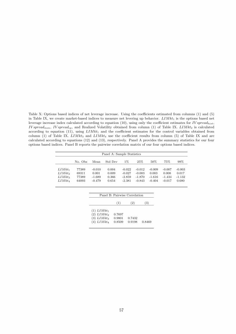
Table X: Options based indices of net leverage increase. Using the coefficients estimated from columns (1) and (5)in Table IX, we create market-based indices to measure net levering up behavior. LIMkt1 is the options based netleverage increase index calculated according to equation (10), using only the coefficient estimates for IV spreadhist,IV spreadmon, IV spreadcp, and Realized Volatility obtained from column (1) of Table IX. LIMkt2 is calculatedaccording to equation (11), using LIMkt1 and the coefficient estimates for the control variables obtained fromcolumn (1) of Table IX. LIMkt3 and LIMkt4 use the coefficient results from column (5) of Table IX and arecalculated according to equations (12) and (13), respectively. Panel A provides the summary statistics for our fouroptions based indices. Panel B reports the pairwise correlation matrix of our four options based indices.

Panel A: Sample Statistics

No. Obs Mean Std Dev 1% 25% 50% 75% 99%

LIMkt1 77389 -0.010 0.004 -0.022 -0.012 -0.009 -0.007 -0.003LIMkt2 69311 0.001 0.009 -0.027 -0.003 0.003 0.008 0.017LIMkt3 77389 -1.689 0.366 -2.859 -1.870 -1.616 -1.434 -1.132LIMkt4 64093 -0.479 0.654 -2.381 -0.843 -0.404 -0.017 0.680

Panel B: Pairwise Correlation

(1) (2) (3)

(1) LIMkt1(2) LIMkt2 0.7697(3) LIMkt3 0.9801 0.7432(4) LIMkt4 0.8509 0.9198 0.8469

57

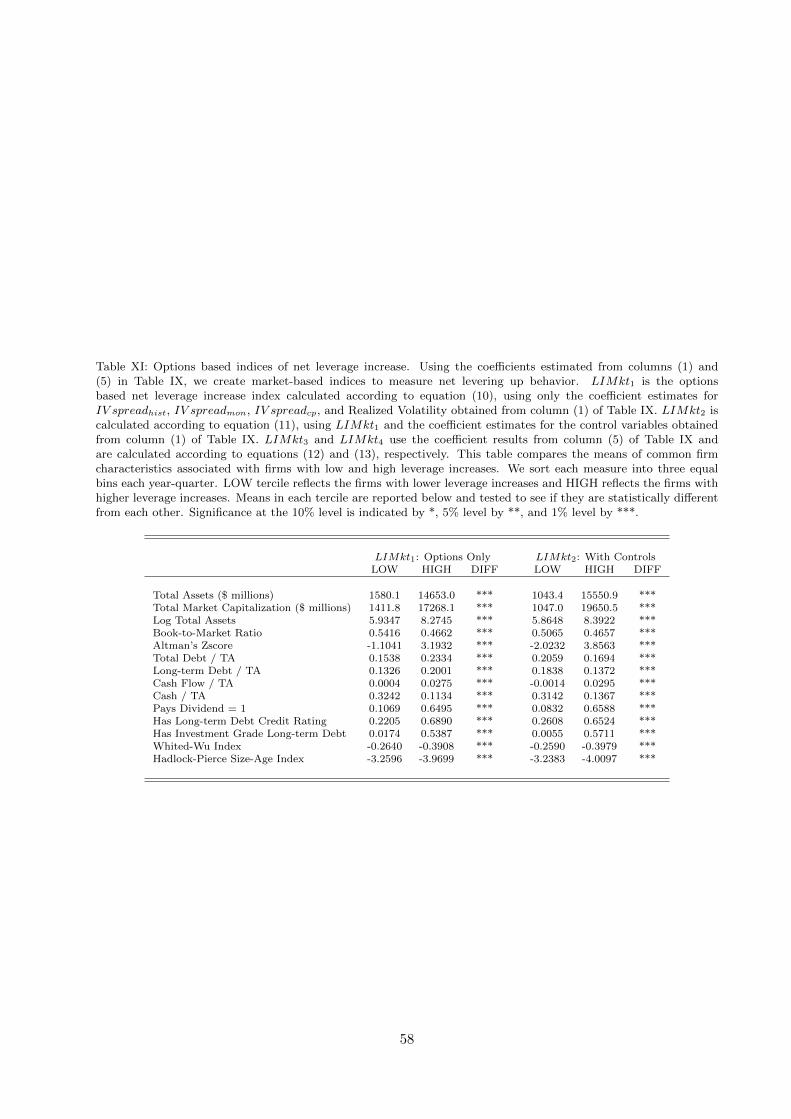
Table XI: Options based indices of net leverage increase. Using the coefficients estimated from columns (1) and(5) in Table IX, we create market-based indices to measure net levering up behavior. LIMkt1 is the optionsbased net leverage increase index calculated according to equation (10), using only the coefficient estimates forIV spreadhist, IV spreadmon, IV spreadcp, and Realized Volatility obtained from column (1) of Table IX. LIMkt2 iscalculated according to equation (11), using LIMkt1 and the coefficient estimates for the control variables obtainedfrom column (1) of Table IX. LIMkt3 and LIMkt4 use the coefficient results from column (5) of Table IX andare calculated according to equations (12) and (13), respectively. This table compares the means of common firmcharacteristics associated with firms with low and high leverage increases. We sort each measure into three equalbins each year-quarter. LOW tercile reflects the firms with lower leverage increases and HIGH reflects the firms withhigher leverage increases. Means in each tercile are reported below and tested to see if they are statistically differentfrom each other. Significance at the 10% level is indicated by *, 5% level by **, and 1% level by ***.

LIMkt1: Options Only LIMkt2: With ControlsLOW HIGH DIFF LOW HIGH DIFF

Total Assets ($ millions) 1580.1 14653.0 *** 1043.4 15550.9 ***Total Market Capitalization ($ millions) 1411.8 17268.1 *** 1047.0 19650.5 ***Log Total Assets 5.9347 8.2745 *** 5.8648 8.3922 ***Book-to-Market Ratio 0.5416 0.4662 *** 0.5065 0.4657 ***Altman’s Zscore -1.1041 3.1932 *** -2.0232 3.8563 ***Total Debt / TA 0.1538 0.2334 *** 0.2059 0.1694 ***Long-term Debt / TA 0.1326 0.2001 *** 0.1838 0.1372 ***Cash Flow / TA 0.0004 0.0275 *** -0.0014 0.0295 ***Cash / TA 0.3242 0.1134 *** 0.3142 0.1367 ***Pays Dividend = 1 0.1069 0.6495 *** 0.0832 0.6588 ***Has Long-term Debt Credit Rating 0.2205 0.6890 *** 0.2608 0.6524 ***Has Investment Grade Long-term Debt 0.0174 0.5387 *** 0.0055 0.5711 ***Whited-Wu Index -0.2640 -0.3908 *** -0.2590 -0.3979 ***Hadlock-Pierce Size-Age Index -3.2596 -3.9699 *** -3.2383 -4.0097 ***

58

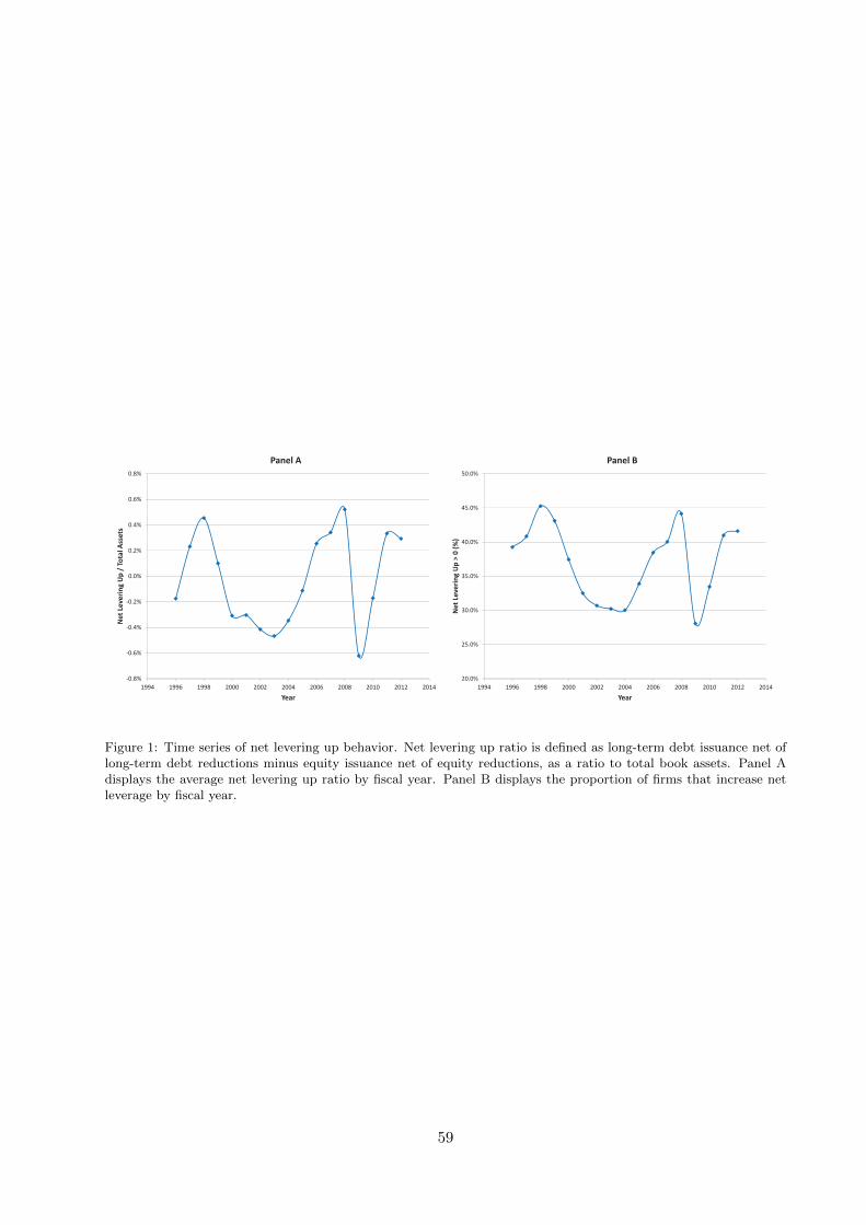
0.8%

0.6%

0.4%

0.2%

0.0%

0.2%

0.4%

0.6%

0.8%

1994 1996 1998 2000 2002 2004 2006 2008 2010 2012 2014

NetLeveringUp/TotalAssets

Year

Panel A

20.0%

25.0%

30.0%

35.0%

40.0%

45.0%

50.0%

1994 1996 1998 2000 2002 2004 2006 2008 2010 2012 2014

NetLeveringUp>0(%

)

Year

Panel B

Figure 1: Time series of net levering up behavior. Net levering up ratio is defined as long-term debt issuance net oflong-term debt reductions minus equity issuance net of equity reductions, as a ratio to total book assets. Panel Adisplays the average net levering up ratio by fiscal year. Panel B displays the proportion of firms that increase netleverage by fiscal year.

59

Table

XII

:P

ort

folio

analy

sis

base

don

equal-

wei

ghte

dand

valu

e-w

eighte

dp

ort

folios

of

lever

age

incr

ease

.W

eso

rtfirm

sbase

don

our

four

mark

et-b

ase

dm

easu

res

of

lever

age

incr

ease

,LIMkt 1

thro

ughLIMkt 4

,in

tote

rciles

each

month

.F

irm

sth

at

fall

into

the

top

(bott

om

)te

rcile

are

class

ified

as

hav

ing

hig

her

lever

age

incr

ease

s(l

ower

lever

ages

).F

orm

ing

port

folios

from

each

terc

ile,

we

find

the

equal-

wei

ghte

dav

erage

retu

rnin

each

port

folio

and

regre

ssth

eti

me-

seri

esof

the

port

folio

retu

rns

on

the

Past

or

and

Sta

mbaugh

(2003)

5-f

act

or

model

inco

lum

ns

(1)

thro

ugh

(4).

We

use

the

valu

e-w

eighte

dre

turn

inea

chp

ort

folio

inth

e5-f

act

or

model

inco

lum

ns

(5)

thro

ugh

(8).

Panel

Apre

sents

the

full

resu

lts

for

the

zero

-cost

Low

-Hig

hp

ort

folio.

Panel

sB

and

Cre

port

the

Alp

has

from

the

fact

or

regre

ssio

nfo

rth

eL

owand

Hig

hp

ort

folios,

resp

ecti

vel

y.Sta

ndard

erro

rsare

rep

ort

edin

the

pare

nth

eses

.Sig

nifi

cance

at

the

10%

level

isin

dic

ate

dby

*,

5%

level

by

**,

and

1%

level

by

***.

LIM

kt 1

LIM

kt 2

LIM

kt 3

LIM

kt 4

LIM

kt 1

LIM

kt 2

LIM

kt 3

LIM

kt 4

EW

EW

EW

EW

VW

VW

VW

VW

(1)

(2)

(3)

(4)

(5)

(6)

(7)

(8)

Pan

elA

:L

ow

-Hig

hP

ort

folio

Alp

ha

-0.0

098

***

-0.0

154

***

-0.0

139

***

-0.0

148

***

0.0

085

**

-0.0

011

0.0

000

-0.0

009

(0.0

030)

(0.0

030)

(0.0

031)

(0.0

032)

(0.0

043)

(0.0

039)

(0.0

043)

(0.0

049)

No.

Ob

s.153

153

153

153

153

153

153

153

R2

0.6

554

0.5

663

0.6

767

0.5

863

0.3

769

0.4

404

0.4

687

0.3

826

Pan

elB

:L

ow

Port

folio

Alp

ha

-0.0

085

***

-0.0

115

***

-0.0

105

***

-0.0

111

***

0.0

126

***

0.0

061

**

0.0

053

0.0

067

*(0

.0021)

(0.0

021)

(0.0

023)

(0.0

023)

(0.0

036)

(0.0

027)

(0.0

035)

(0.0

035)

No.

Ob

s.153

153

153

153

153

153

153

153

R2

0.9

250

0.9

102

0.9

174

0.9

060

0.8

067

0.8

662

0.8

394

0.8

353

Pan

elC

:H

igh

Port

folio

Alp

ha

0.0

013

0.0

039

**

0.0

034

**

0.0

037

**

0.0

042

**

0.0

072

***

0.0

053

***

0.0

077

***

(0.0

016)

(0.0

016)

(0.0

015)

(0.0

016)

(0.0

019)

(0.0

023)

(0.0

019)

(0.0

024)

No.

Ob

s.153

153

153

153

153

153

153

153

R2

0.8

811

0.8

744

0.8

748

0.8

744

0.7

544

0.6

981

0.7

429

0.6

838

60

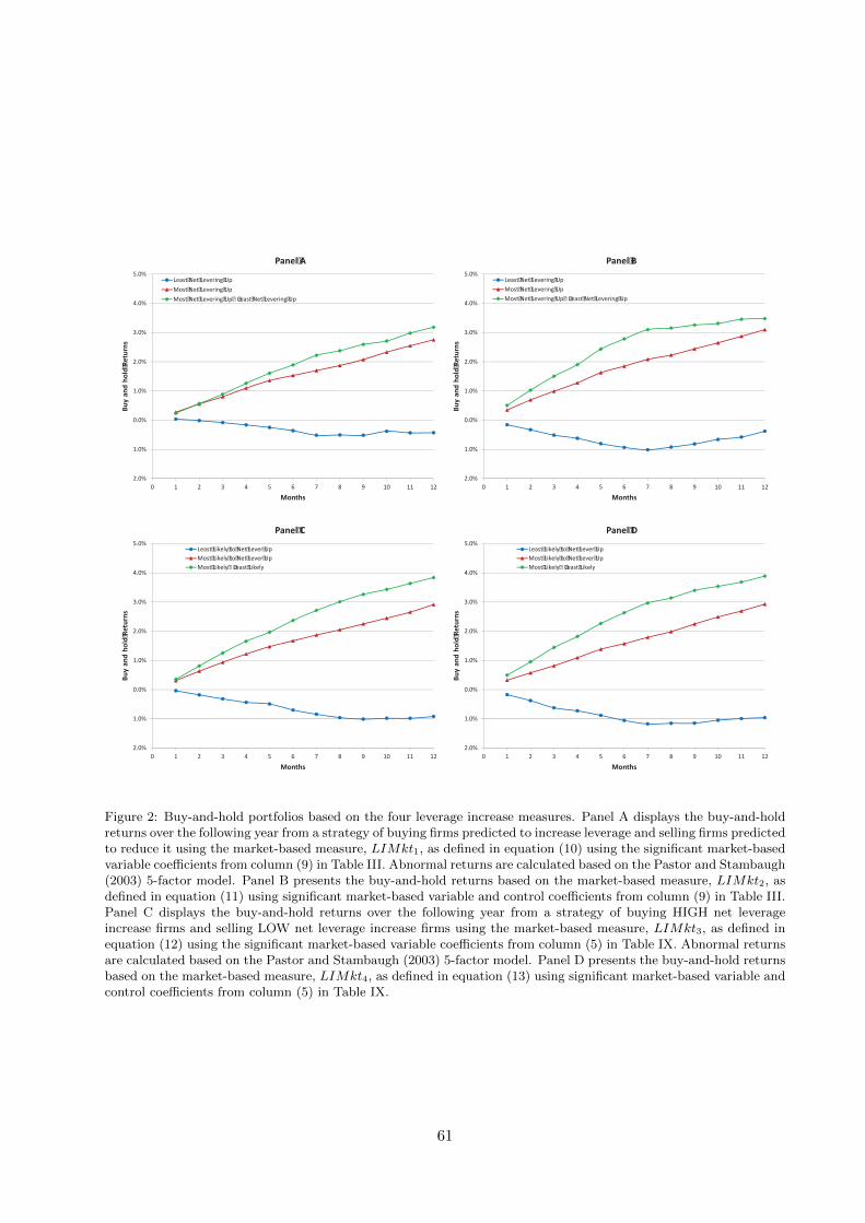
2.0%

1.0%

0.0%

1.0%

2.0%

3.0%

4.0%

5.0%

0 1 2 3 4 5 6 7 8 9 10 11 12

Buyandhold

Returns

Months

Panel A

Least Net Levering Up

Most Net Levering Up

Most Net Levering Up Least Net Levering Up

2.0%

1.0%

0.0%

1.0%

2.0%

3.0%

4.0%

5.0%

0 1 2 3 4 5 6 7 8 9 10 11 12

Buyandhold

Returns

Months

Panel B

Least Net Levering Up

Most Net Levering Up

Most Net Levering Up Least Net Levering Up

2.0%

1.0%

0.0%

1.0%

2.0%

3.0%

4.0%

5.0%

0 1 2 3 4 5 6 7 8 9 10 11 12

Buyandhold

Returns

Months

Panel C

Least Likely to Net Lever Up

Most Likely to Net Lever Up

Most Likely Least Likely

2.0%

1.0%

0.0%

1.0%

2.0%

3.0%

4.0%

5.0%

0 1 2 3 4 5 6 7 8 9 10 11 12

Buyandhold

Returns

Months

Panel D

Least Likely to Net Lever Up

Most Likely to Net Lever Up

Most Likely Least Likely

Figure 2: Buy-and-hold portfolios based on the four leverage increase measures. Panel A displays the buy-and-holdreturns over the following year from a strategy of buying firms predicted to increase leverage and selling firms predictedto reduce it using the market-based measure, LIMkt1, as defined in equation (10) using the significant market-basedvariable coefficients from column (9) in Table III. Abnormal returns are calculated based on the Pastor and Stambaugh(2003) 5-factor model. Panel B presents the buy-and-hold returns based on the market-based measure, LIMkt2, asdefined in equation (11) using significant market-based variable and control coefficients from column (9) in Table III.Panel C displays the buy-and-hold returns over the following year from a strategy of buying HIGH net leverageincrease firms and selling LOW net leverage increase firms using the market-based measure, LIMkt3, as defined inequation (12) using the significant market-based variable coefficients from column (5) in Table IX. Abnormal returnsare calculated based on the Pastor and Stambaugh (2003) 5-factor model. Panel D presents the buy-and-hold returnsbased on the market-based measure, LIMkt4, as defined in equation (13) using significant market-based variable andcontrol coefficients from column (5) in Table IX.

61