Embed Size (px)
Citation preview

Options ValuationOptions Valuation
Chapter 21Chapter 21
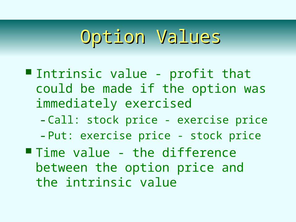
Intrinsic value - profit that could be made if the option was immediately exercised- Call: stock price - exercise price
- Put: exercise price - stock price Time value - the difference between the
option price and the intrinsic value
Option ValuesOption Values
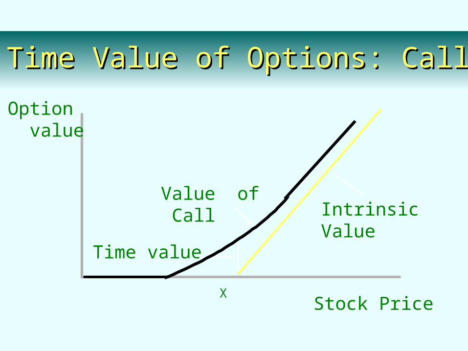
Time Value of Options: CallTime Value of Options: Call
Option value
XStock Price
Value of Call Intrinsic Value
Time value

Factor Effect on value
Stock price increases
Exercise price decreases
Volatility of stock price increases
Time to expiration increases
Interest rate increases
Dividend Rate decreases
Factors Influencing Option Values: Factors Influencing Option Values: CallsCalls
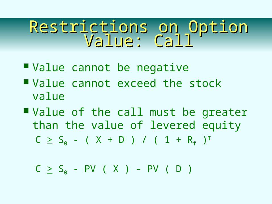
Restrictions on Option Value: CallRestrictions on Option Value: Call
Value cannot be negative Value cannot exceed the stock value Value of the call must be greater than the
value of levered equityC > S0 - ( X + D ) / ( 1 + Rf )T
C > S0 - PV ( X ) - PV ( D )
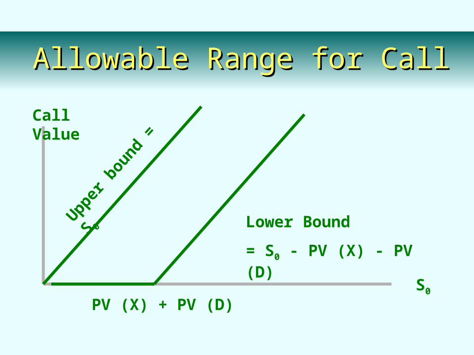
Allowable Range for CallAllowable Range for Call
Call Value
S0
PV (X) + PV (D)
Upper
bou
nd =
S 0
Lower Bound
= S0 - PV (X) - PV (D)

100
200
50
Stock Price
C
75
0
Call Option Value X = 125
Binomial Option Pricing:Binomial Option Pricing:Text ExampleText Example

Alternative Portfolio
Buy 1 share of stock at $100
Borrow $46.30 (8% Rate)
Net outlay $53.70
Payoff
Value of Stock 50 200
Repay loan - 50 -50
Net Payoff 0 150
53.70
150
0
Payoff Structureis exactly 2 timesthe Call
Binomial Option Pricing:Binomial Option Pricing:Text ExampleText Example
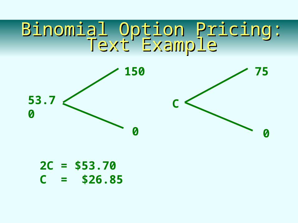
53.70
150
0
C
75
0
2C = $53.70C = $26.85
Binomial Option Pricing:Binomial Option Pricing:Text ExampleText Example

Alternative Portfolio - one share of stock and 2 calls written (X = 125)
Portfolio is perfectly hedged
Stock Value 50 200
Call Obligation 0 -150
Net payoff 50 50
Hence 100 - 2C = 46.30 or C = 26.85
Another View of Replication of Another View of Replication of Payoffs and Option ValuesPayoffs and Option Values

Generalizing the Generalizing the Two-State ApproachTwo-State Approach
Assume that we can break the year into two six-month segments
In each six-month segment the stock could increase by 10% or decrease by 5%
Assume the stock is initially selling at 100
Possible outcomes
Increase by 10% twice
Decrease by 5% twice
Increase once and decrease once (2 paths)
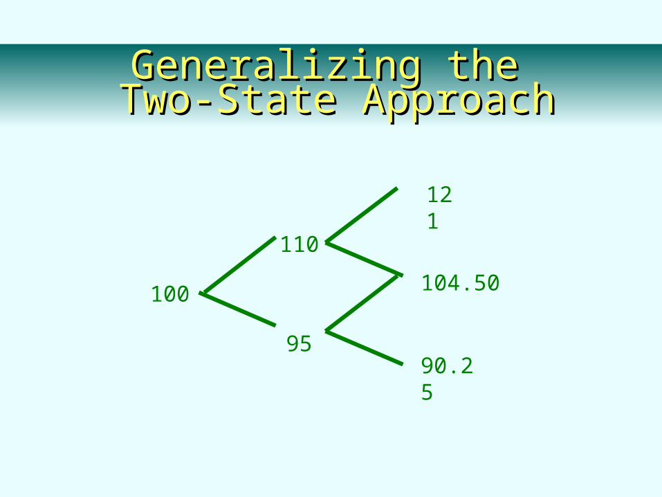
Generalizing the Generalizing the Two-State ApproachTwo-State Approach
100
110
121
9590.25
104.50
Assume that we can break the year into three intervals
For each interval the stock could increase by 5% or decrease by 3%
Assume the stock is initially selling at 100
Expanding to Expanding to Consider Three IntervalsConsider Three Intervals
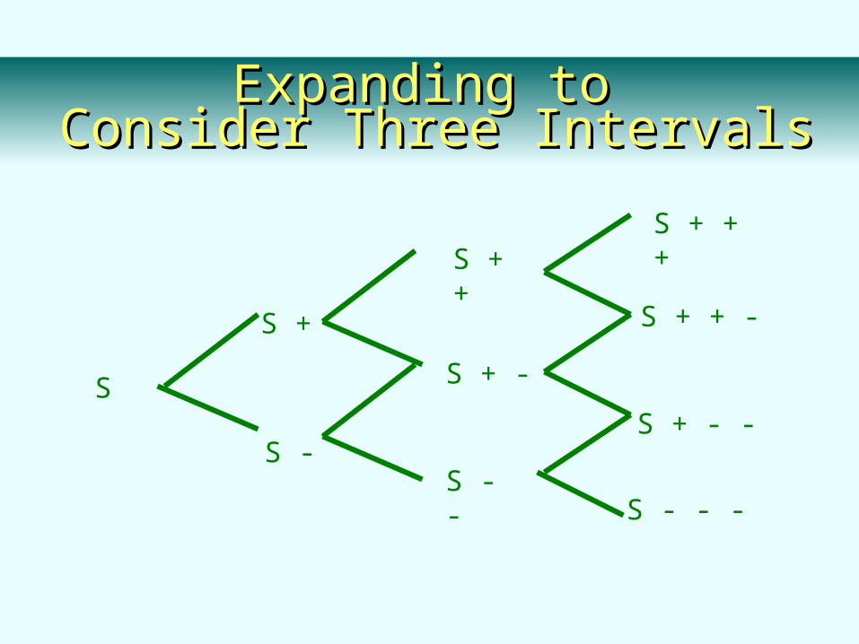
S
S +
S + +
S -S - -
S + -
S + + +
S + + -
S + - -
S - - -
Expanding to Expanding to Consider Three IntervalsConsider Three Intervals
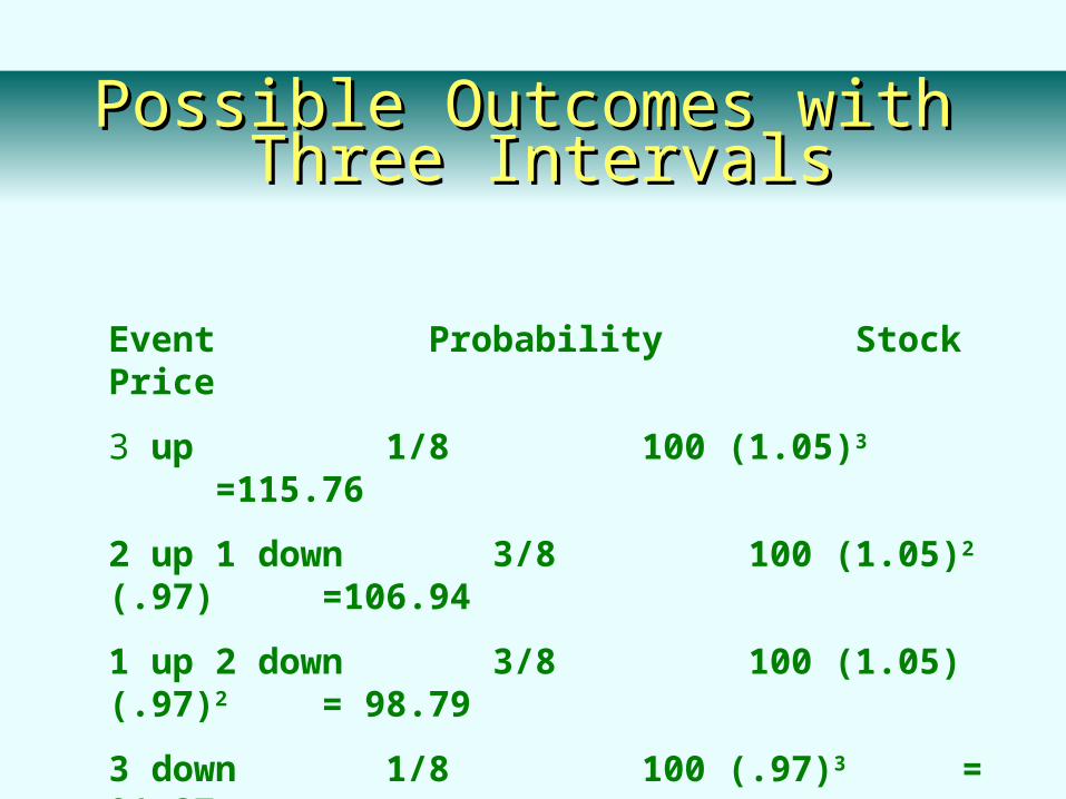
Possible Outcomes with Possible Outcomes with Three IntervalsThree Intervals
Event Probability Stock Price
3 up 1/8 100 (1.05)3 =115.76
2 up 1 down 3/8 100 (1.05)2 (.97) =106.94
1 up 2 down 3/8 100 (1.05) (.97)2 = 98.79
3 down 1/8 100 (.97)3 = 91.27

Co = SoN(d1) - Xe-rTN(d2)
d1 = [ln(So/X) + (r + 2/2)T] / (T1/2)
d2 = d1 + (T1/2)
whereCo = Current call option value.
So = Current stock price
N(d) = probability that a random draw from a normal dist. will be less than d.
Black-Scholes Option ValuationBlack-Scholes Option Valuation
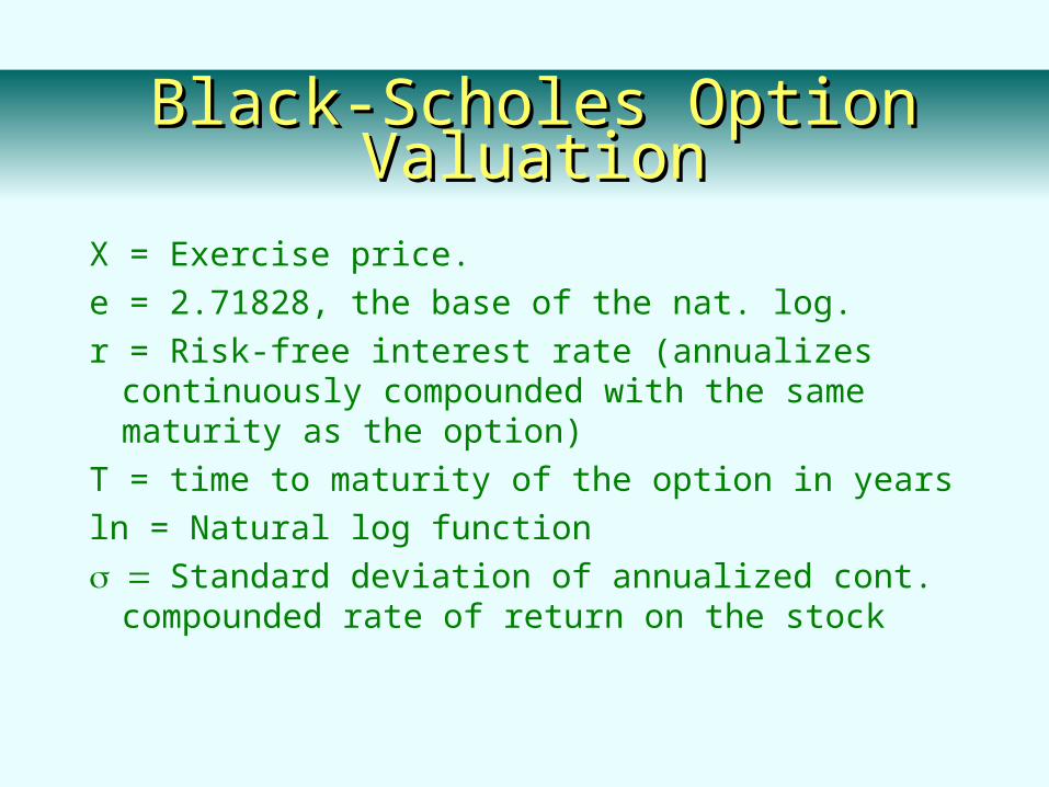
X = Exercise price.
e = 2.71828, the base of the nat. log.
r = Risk-free interest rate (annualizes continuously compounded with the same maturity as the option)
T = time to maturity of the option in years
ln = Natural log function
Standard deviation of annualized cont. compounded rate of return on the stock
Black-Scholes Option ValuationBlack-Scholes Option Valuation
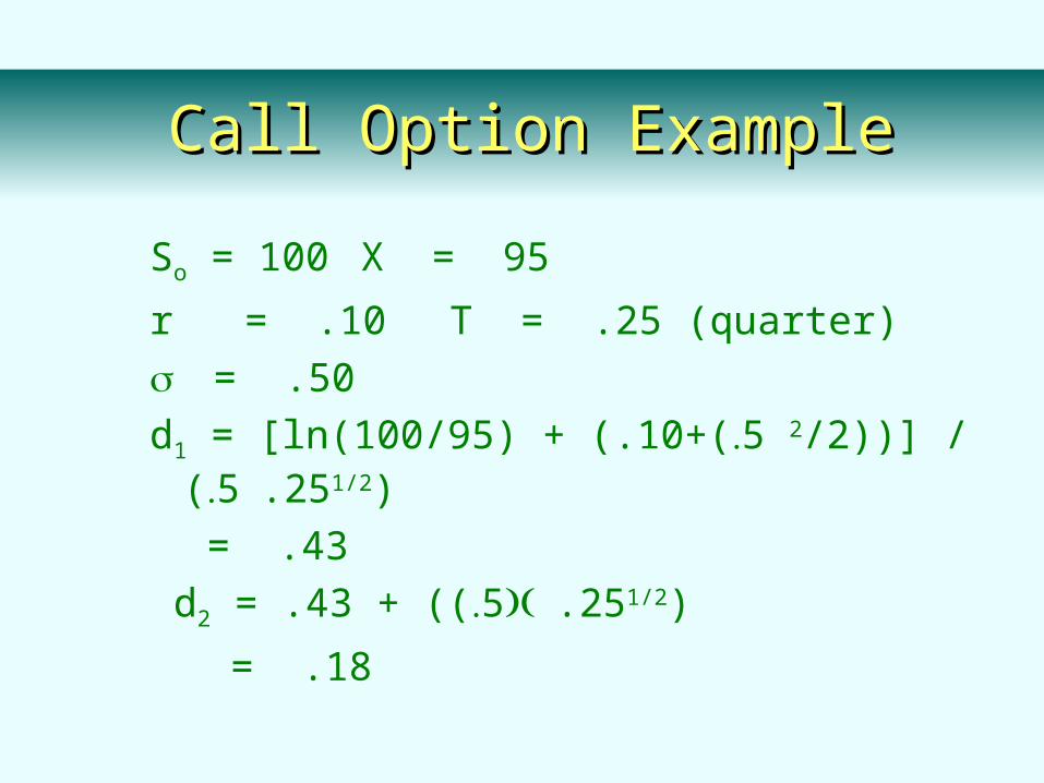
So = 100 X = 95
r = .10 T = .25 (quarter)
= .50
d1 = [ln(100/95) + (.10+(5 2/2))] / (5.251/2)
= .43
d2 = .43 + ((5.251/2)
= .18
Call Option ExampleCall Option Example
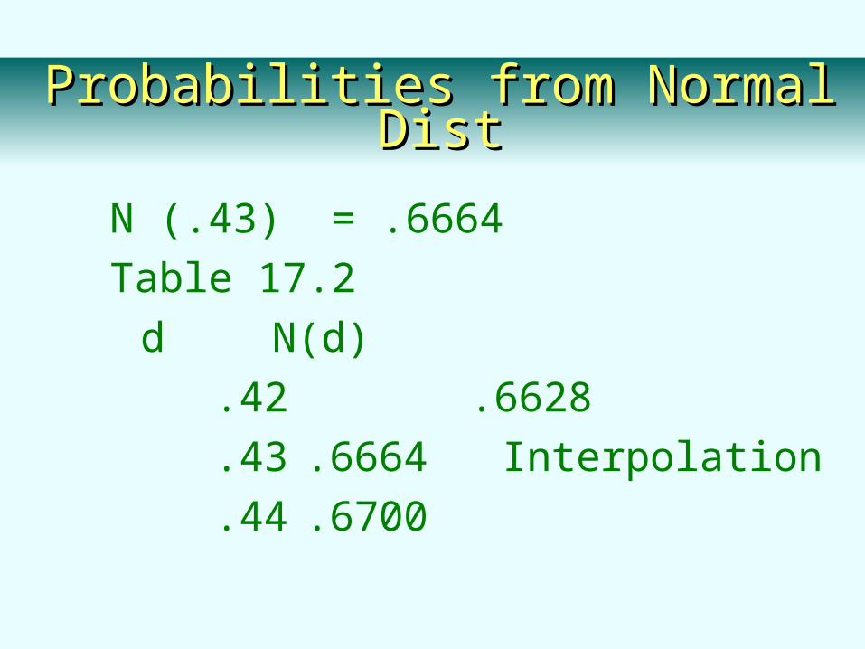
N (.43) = .6664
Table 17.2
d N(d)
.42 .6628
.43 .6664 Interpolation
.44 .6700
Probabilities from Normal DistProbabilities from Normal Dist
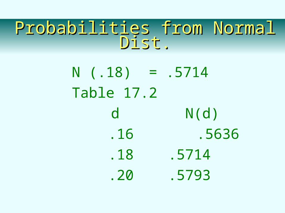
N (.18) = .5714
Table 17.2
d N(d)
.16 .5636
.18 .5714
.20 .5793
Probabilities from Normal Dist.Probabilities from Normal Dist.

Co = SoN(d1) - Xe-rTN(d2)
Co = 100 X .6664 - 95 e- .10 X .25 X .5714
Co = 13.70
Implied Volatility
Using Black-Scholes and the actual price of the option, solve for volatility.
Is the implied volatility consistent with the stock?
Call Option ValueCall Option Value
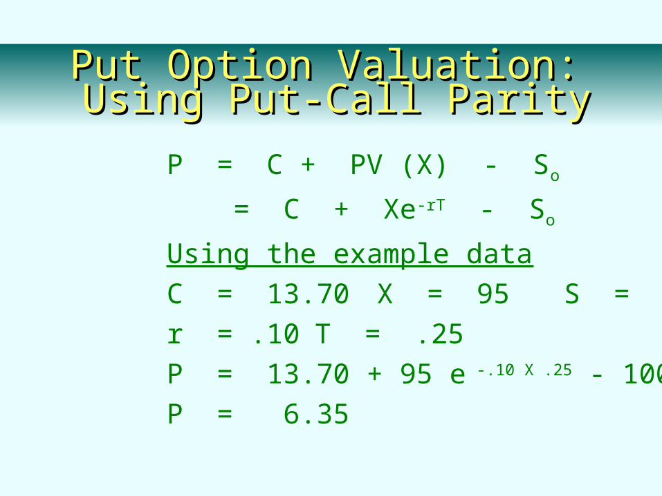
P = C + PV (X) - So
= C + Xe-rT - So
Using the example data
C = 13.70 X = 95 S = 100
r = .10 T = .25
P = 13.70 + 95 e -.10 X .25 - 100
P = 6.35
Put Option Valuation: Put Option Valuation: Using Put-Call ParityUsing Put-Call Parity

Adjusting the Black-Scholes Adjusting the Black-Scholes Model for DividendsModel for Dividends
The call option formula applies to stocks that pay dividends
One approach is to replace the stock price with a dividend adjusted stock priceReplace S0 with S0 - PV (Dividends)

Hedging: Hedge ratio or delta The number of stocks required to hedge against the price
risk of holding one option
Call = N (d1)
Put = N (d1) - 1
Option Elasticity
Percentage change in the option’s value given a 1% change in the value of the underlying stock
Using the Black-Scholes FormulaUsing the Black-Scholes Formula
Buying Puts - results in downside protection with unlimited upside potential
Limitations - Tracking errors if indexes are used for the puts
- Maturity of puts may be too short
- Hedge ratios or deltas change as stock values change
Portfolio Insurance - Protecting Portfolio Insurance - Protecting Against Declines in Stock ValueAgainst Declines in Stock Value