OR-20-014 Optimize a Chilled-Water Plant with Magnetic ... · gal chillers are more efficient than the original chillers, espe-ciallyatlowerloads.Athighloadratio,theefficiencybenefit

© 2020 ASHRAE. THIS PREPRINT MAY NOT BE DISTRIBUTED IN PAPER OR DIGITAL FORM IN WHOLE OR IN PART. IT IS FOR DISCUSSION PURPOSES ONLYAT THE 2019 ASHRAE WINTER CONFERENCE. The archival version of this paper along with comments and author responses will be published in ASHRAETransactions, Volume 126, Part 1. ASHRAE must receive written questions or comments regarding this paper by February 21, 2020, for them to be included inTransactions.

ABSTRACT

Variable speed centrifugal chillers perform much moreefficiently at part-load ratio of cooling demand as well aspartial compression ratio of lift head compared to constantspeed centrifugal chillers. Magnetic bearing technologyfurther improves the benefit of variable speed centrifugalchillers. This performance difference requires a reconsider-ation of most effective plant operation when magnetic bearingcentrifugal chillers are incorporated. In this paper, a compo-nent-based model is developed for a chilled-water plant withoil-free chillers at the Texas A&M University System RELLISCampus. The model, calibrated by on-site measured data fromthe building automation system, is used to evaluate the savingspotential for different operation strategies. An optimal chillerstagingstrategy,basedon theoptimalefficiencycurve, is simu-lated for the case study plant under constant water flow andvariable water flow scenarios respectively. The results showthat optimal chiller staging only improves plant performanceby 2.1% for the constant water flow system. Implementing opti-mal staging with variable water flow would increase theenergy savings to 13.7% compared to current operation of thecase-study plant.

INTRODUCTION

Magnetic bearing centrifugal chillers with variable-speeddrives (VSD), also known as oil-free centrifugal chillers,allow the centrifugal compressors to operate without the use ofoil for lubrication, which reduces energy losses due to frictionand increases the heat transfer efficiency in the chiller, becauseno oil enters the evaporator or condenser. A variable speeddrive on the motor allows the compressor to operate muchmore efficiently at partial loads than standard compressors.

The oil-free system also eliminates the need for oil mainte-nance, resulting in operations and maintenance savings. Whencompared to a conventional centrifugal chiller with VSD, Yuand Chan [2015] determined that oil lubrication-based opera-tions suffered from a 3.2% performance decrease in the chilleras well as accelerated performance degradation.

Furthermore, because there is no limitation on the mini-mum compression ratio for the oil return system, magneticbearing centrifugal chillers are capable of operating withlower condenser water supply temperatures compared to someconventional compressor systems. This results in an additionalimprovement in efficiency and higher capacity. Somemagnetic bearing chillers are also able to operate continuouslywith minimum entering condenser water temperature belowthe leaving chilled-water set point. This is sometimes referredto as inverted or upside down operation. It can operate stablywith an entering condenser water temperature 35.0°F (1.7°C),below the leaving chilled-water set point. Because free cool-ing is not so free anymore, these new chillers lower costs byeliminating the need for water-to-water heat exchangers andtheir accompanying expenses, such as piping controls andoperation and maintenance expenses.

Deng [2018] examines actual performance of MagneticBearing Centrifugal Chillers in different buildings and citiesthrough a whole year and compares the results to those ofconventional centrifugal chillers. It was found that magneticbearing centrifugal chillers clearly performed much more effi-ciently, especially at part-load ratio as well as partial compres-sion ratio. Thus, to fully take advantage of magnetic bearingcentrifugal chillers for truly energy efficient operation, onemust optimize a magnetic bearing centrifugal chiller’s opera-tion based on an annual hourly simulation of cooling demand

Optimize a Chilled-Water Plant withMagnetic-Bearing Variable Speed Chillers

Lei Wang, PhD, PE Yasuko Sakurai, DEng David E. Claridge, PhD, PEMember ASHRAE Fellow ASHRAE

Lei Wang is an energy analyst in Utilities and Energy Services, Yasuko Sakurai is Manager of Analytical Service in Utilities and EnergyServices; and David E. Claridge is director of the Texas A&M Engineering Experiment Station (TEES) Energy Systems Laboratory, andLeland Jordan Professor of Mechanical Engineering at Texas A&M University, College Station, TX.

OR-20-014

PREPRINT ONLY. ASHRAE allows authors to post their ASHRAE-published paper onto their personal & company’s website once the final version has been published.

2 OR-20-014

and compression ratio demand rather than just thinking of thenominal rated conditions.

Li [2004] claimed that the key contributor to poor chillerplant performance was the mismatch between the demand andsupply sides. Due to improper cooling load calculations orunreasonable safety factors, oversized chiller capacities havebecome a common phenomenon in HVAC systems. Even aperfectly designed chiller plant could be very significantlyoversized in actual operation since the cooling load reaches itspeak level for only a small proportion of time in each year(Cheng [2017]). This oversized cooling capacity decreasesoperational energy performance and wastes energy through-out the cooling season (Woradechjumroen [2014], Djunaedy[2011]) for conventional chillers. However, a magnetic bear-ing variable speed centrifugal chiller may solve this mismatchissue, because it can operate much more efficiently at partialloads than conventional compressors. Guo [2014], analyzedthe energy saving rate of a data center by replacing conven-tional chillers with magnetic bearing centrifugal chillers.Results showed a 37% (minimum) reduction in energyconsumption. However, Guo relied on four discrete designvalues of the Integrated Part-Load Value (IPLV) to calculatethe energy-savings instead of using an actual load profile. TheIPLV assumes the entering condenser water temperature isdropping with load. This operating profile allows compressionspeed requirements for flow and lift head to decline togetherreducing the need for mechanical unloaders or over compres-sion. If chillers run only at these four discrete operating pointsthis would be appropriate, but this is rarely the case. AHRI550/590 [2011] advises that IPLV “was derived to provide arepresentation of the average part-load efficiency for a single

chiller only”. Most chilled-water plants employ more than onechiller to meet the load. The IPLV rarely depicts an actualchiller’s load profile because most chiller plants have morethan one chiller and the local weather likely does not match thestandard AHRI profile. Carrier [2015] stated that the reality ofactual operation is much less elegant than IPLV, resulting inoperating points where the use of mechanical unloaders orover compression are more likely to occur. This is because theactual operating points are further from the ideal speed curvethan the operating points in the AHRI IPLV load profile.

Hartman [2001] developed operating strategies toenhance performance of all-variable speed chillers in comfortconditioning chiller plant applications. Optimum overallchiller plant performance is achieved when the rate of plantmarginal capacity versus marginal power use is the same foreach element of the system.

Parker [2012] assessed operation of variable-speedmagnetic bearing centrifugal chillers with magnetic bearings.The monitored data show the new magnetic bearing centrifu-gal chillers are more efficient than the original chillers, espe-cially at lower loads. At high load ratio, the efficiency benefitis measurable, but is not as significant. However, as the loadratio decreases, the efficiency benefit becomes morepronounced. Therefore, this report recommended improvingchiller-staging controls. If multiple chillers were available, itmay reduce total chiller plant power by operating two chillersat half load rather than a single chiller at full load.

Figure 1 shows a performance comparison of constant,variable speed and magnetic bearing variable speed centrifu-gal chillers at different load conditions. Constant speedchillers have a relatively flat performance curve across a range

Figure 1 Performance comparison of constant-speed, variable-speed, and magnetic-bearing variable-speed centrifugalchillers.


OR-20-014 3

of load conditions; therefore, the focus of constant speedchiller plant operation has been minimizing the amount of on-line equipment. This permits chillers to operate as close aspossible to their full capacity to reduce the percent of auxiliaryelectricity consumption from water pumps and cooling towerfans that are usually sequenced with chillers. However,Figure 1 also shows that Variable Speed (VS) chillers andMagnetic Bearing Variable Speed (MBVS) chillers operatemost efficiently well below full load. The efficiency improve-ment of MBVS chillers can be very substantial at lowcondenser water temperatures. Part of the improved part-loadefficiency curve for MBVS chillers is the change in motortype, with higher motor efficiency at part load and allowing theelimination of gear losses, not only the reduction of frictionallosses in bearings. One should also note that the condenserwater temperatures listed in Figure 1 are per AHRI 550/590condenser relief assumptions. They are for rating purpose onlyand actual condenser water temperatures will not always varywith load as shown.

These performance differences require reconsideration ofthe most efficient operation strategy for a plant using magneticbearing variable speed centrifugal chillers. In this paper, acomponent-based model is developed for a chilled-water plantwith magnetic bearing centrifugal chillers at the Texas A&MUniversity System RELLIS Campus, in Bryan. The models,calibrated by on-site measured data from the building automa-tion system, are used to evaluate the savings potential fordifferent operation strategies.

CENTRIFUGAL CHILLERS PERFORMANCE CURVE

All centrifugal compressors (regardless of bearing type,refrigerant type, motor type, oiled or oil free) must generallyadhere to the ideal fan laws, illustrated in Figure 2 [Carrier,2015].

a. First law: Mass flow (capacity) is linear with speed.b. Second law: Lift (ability to generate head) increases with

the square of speed.c. Third law: Power increases with the cube of speed. (It

may be less than cubic due to the proximity of guidevanes to the impeller inlet.)

In simple terms, the ability to generate head in a centrif-ugal compressor is related to the square of speed. At 80%speed, a centrifugal will generate 80%×80%=64% of itsdesign head. If the operating condition requires more than64% of design head, the centrifugal compressor will surge.Centrifugal compressors move gas through an open pathbetween the low-pressure evaporator to the higher-pressurecondenser. If the pressure difference (head) is too large, flowreversal will occur (surge).

To avoid surge, the centrifugal compressor must eitherspeed up or engage hot gas bypass (also called load balancevalves or recirculation flow on many magnetic bearingmachines). So, while we may be inclined to believe thatcompressor speed is typically based on capacity, it is actuallyoften based on the head required. For example, if a chiller isoperating at 50% load and 75.0°F (23.9°C) entering condenserwater, the first law would suggest we could operate at 50%speed, but the 2nd law requires us to run at 84% speed.

(1)

This raises an interesting question: If the centrifugalcompressor must operate at 84% speed to develop sufficienthead; how do we limit the capacity to 50%? This requires anunloading device such as inlet guide vanes, discharge flowrestrictions, load balance valves (hot gas bypass) or someother means of diverting or restricting flow. The net result isthe compressor is compressing more refrigerant or head thanis required to meet the load, which represents an increase inpower per unit of cooling at the operating point.

The ideal fan laws define a minimum speed requirementfor flow and a separate minimum speed requirement for thegeneration of head in a centrifugal compressor. Combiningthese two minimum speed requirements, it becomes apparentthat the ideal speed for a centrifugal compressor occurs whenthe speed required for mass flow exactly matches the speedrequired to generate head (as shown in Figure 3). Above this

Figure 2 Ideal fan laws.

%LiftCWETactual T actual CHWLTactual–+

CWETdesign T design CHWLTdesign–+-------------------------------------------------------------------------------------------------------=

%Lift 75°F 5°F 44°F–+85°F 10°F 44°F–+------------------------------------------------- 36°F

51°F------------ 71%= = =

%Speed 71% 84%= =


4 OR-20-014

speed, the high head forces the centrifugal compressor to oper-ate at higher speeds than needed for capacity and mechanicalunloaders are employed. Below this speed, the speed for massflow exceeds the head requirements resulting in over-compression. In either case, the performance of the centrifugalchiller will decrease. The further the operating point is fromthe ideal speed curve, the greater the impact will be. Figure 4illustrates the optimal efficiency curve for the case study ofone particular model of MBVS chiller with a single compres-sor.

The optimal efficiency curve of a variable speed chillerwhen operating with a fixed chilled-water supply temperatureis a simple concept. It is the locus of points of highest chilleroperating efficiency at various condenser water temperatureand load conditions. In other words, the speed required formass flow exactly matches the speed required to generatehead. Notice that the best efficiency (lowest kW/ton) for theoil-free variable speed centrifugal chiller when the entering

condenser water temperature is 85.0°F (29.4°C) is achieved atabout 58% load. This is the point on the optimal efficiencycurve for that condensing water temperature. The optimal effi-ciency curve is developed by connecting the points of highestefficiency for each condensing water temperature. In Figure 4,the performance curves are for constant condenser water andchilled-water flows. For applications where chilled-watertemperature is variable or condenser water flow is varied, anew optimal efficiency curve can be constructed by using lifttemperature head, which is the difference between leavingchilled-water temperature and leaving condenser watertemperature. The optimal load ratio is the fraction of thedesign maximum capacity at which the chiller will be operat-ing on its optimal efficiency curve at the current lift headconditions. One needs to notice that the “ideal centrifugalspeed curve” (Figure 3) and the “optimal efficiency curve”(Figure 4) are unique to a specific chiller model and that such

Figure 3 Ideal centrifugal speed.

Figure 4 Chiller performance and optimal efficiency curves.


OR-20-014 5

curves will vary from model to model due to chiller perfor-mance changes.

The operation of a chilled-water plant should be close tothe optimal efficiency curve to improve chiller efficiency.However, higher chiller efficiency will not guarantee optimumoverall chiller plant performance. The operation of chilled-water pumps, condenser pumps and tower fans that serve eachon-line chiller also affects the overall plant performance.

DESIGN INFORMATION

The case-study plant consists of four magnetic-bearingvariable-speed centrifugal chillers, four variable-speedcondenser water pumps, four variable speed chilled-waterpumps and four induced draft type cooling towers with vari-able speed fans. One chilled-water pump, one condenser waterpump and one cooling tower is energized for each chillerstaged on. This control sequence is not optimum; Taylor[2012] suggested a better operation strategy to run as manytower cells as allowed by the minimum flow. The speed ofchilled-water pumps and a bypass valve are modulated tomaintain the chilled-water flow set point. The fan speed ismodulated to maintain the tower cooling water leavingtemperature (CWLT) set point. The condenser water (CW)flow rate can be adjusted by changing CW pump speed. Thechiller is controlled to maintain a constant chilled-water leav-ing temperature.

The design information for the chillers, pumps and cool-ing towers is presented in Table 1, Table 2, and Table 3, respec-tively.

MODELS AND ASSUMPTIONS

A variable speed chiller model is developed based onmanufacturer’s performance data. The coefficient of determi-nation r2 is 0.9928.

(2)

where

X = chiller partial load ratio (0.10 X 1.05)

Y = chiller lift ratio(CWLT – CHWLT)/Design Lift (0.20 Y 1.05)

Although the water flow rates are not input for this model,the effect of variable water flow can be captured by the CWLTandCHWLT.Forexample,whencondenserwater flowfalls, theCWLT will rise, resulting in higher chiller energy consumption.Taylor [2011] found that the variable condenser water flowmight make plant efficiency worse if not properly controlledbecause of this effect. Therefore, CWLT is selected as an inputto simulate this effect. The minimum flow ratios of chilled waterand condenser water are 45% and 60% respectively.

COOLING TOWER MODELING

The mass and heat transfer process in a cooling tower iscomplicated. The effectiveness-NTU model is a popularmodel in cooling tower simulations, but iterations are requiredto obtain a converged solution (Braun, 1989). The overallnumber of transfer units (NTU) can be correlated with thefollowing form:

(3)

where

= water mass flow

= air mass flow

The value of c is between 1.0 and 3.0 for towers, and nranges between –0.4 and –0.8 (Kreider et al., 2002). The cool-ing tower CWLT at the given airflow rate can be calculated byfollowing equation:

PCHLR

Pdesign------------------

0.54838 X– 0.4081x X 2 0.14978Y–+

0.03426Y 2 0.4006 XY 0.0426+ + +=

Figure 5 Optimal load ratio model of case study chiller.

NTU cm· w

m· a-------

1 n+

=

m· w

m· a


6 OR-20-014

(4)

The cooling tower coefficients c (3.00) and n (–0.66) areidentified using the manufacturer’s design data. The root meansquare error (RSME) and normalized root mean square devi-ation (NRMSD) are 1.56°F (0.87°C) and 2.2% respectively.

PUMP AND FAN MODELING

Because the chilled-water pump and condenser waterpump speeds were operating at constant values of 82% and92% respectively, trend data cannot be used to create a regres-sion model. The pump models are developed based on thepumps’ design information and metered power at fixed speed.

CHW Pump power kW model:

PCHWP = 40 × Speed2.75 × 0.745 (5)

CW Pump power kW model:

PCWP = 60 × Speed1.1 × 0.745 (6)

where the speed is normalized to 100% of rated design speed.The CW pump model is not a cubic relationship because

the condenser water loop is an open loop with a fixed towerheight head. When the condenser water flow is reduced, thehead of the condenser pump is not reduced as the power of theflow ratio. Therefore, the condenser water pump model devi-ates from the ideal fan law, where power varies as the cube ofspeed.

COOLING TOWER FAN MODEL

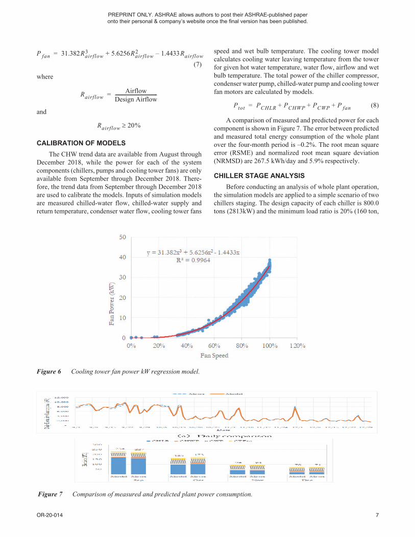
The cooling tower fan power and speed trend data areavailable to develop a fan power model as shown in Figure 6.

Table 1. The Chiller Design Information

CHLRsCapacity CHW Flow CW Flow Efficiency Power Input

Number CompressorTon kW GPM L/S GPM L/S kW/ton COP kW

CHLR 800 2813 1,600 101 2,400 151 0.5868 5.993 469.4 4 Single

Table 2. The Cooling Tower Design Information

CTsDesign water flow

Min. WaterFlow ratio

Entering WaterTemp.

Leaving WaterTemp.

Fan Motor WBNumber

GPM L/S % °F °C °F °C kW °F °C

CT 2400 151 60 95.0 35.0 85.0 29.4 37.25 80.0 26.7 4

Table 3. The Pump Design Information

PumpsDesign Water Flow Head Motor Eff.

NumberGPM L/S ft m hp kW %

CHWP 1600 101 75 23 40 30 84 4

CWP 2400 151 80 24 75 56 80 4

Table 4. Simple Scenario of Chiller Staging for a Two-Chiller Plant

Plant Load Tons, kW Plant Load RatioChiller Load Ratio

Two-Chiller Operation One-Chiller Operation

Load 1 800.0 (2813) 50% 50% 100%

Load 2 640.0 (2251) 40% 40% 80%

Load 3 480.0 (1688) 30% 30% 60%

Load 4 320.0 (1125) 20% 20% 40%

T w o T ref

m· w i T w i T ref– c pw m· a ha o ha i––

m· w oc pw----------------------------------------------------------------------------------------------------+=


OR-20-014 7

(7)

where

and

CALIBRATION OF MODELS

The CHW trend data are available from August throughDecember 2018, while the power for each of the systemcomponents (chillers, pumps and cooling tower fans) are onlyavailable from September through December 2018. There-fore, the trend data from September through December 2018are used to calibrate the models. Inputs of simulation modelsare measured chilled-water flow, chilled-water supply andreturn temperature, condenser water flow, cooling tower fans

speed and wet bulb temperature. The cooling tower modelcalculates cooling water leaving temperature from the towerfor given hot water temperature, water flow, airflow and wetbulb temperature. The total power of the chiller compressor,condenser water pump, chilled-water pump and cooling towerfan motors are calculated by models.

(8)

A comparison of measured and predicted power for eachcomponent is shown in Figure 7. The error between predictedand measured total energy consumption of the whole plantover the four-month period is –0.2%. The root mean squareerror (RSME) and normalized root mean square deviation(NRMSD) are 267.5 kWh/day and 5.9% respectively.

CHILLER STAGE ANALYSIS

Before conducting an analysis of whole plant operation,the simulation models are applied to a simple scenario of twochillers staging. The design capacity of each chiller is 800.0tons (2813kW) and the minimum load ratio is 20% (160 ton,

Figure 6 Cooling tower fan power kW regression model.

Figure 7 Comparison of measured and predicted plant power consumption.

P fan 31.382Rairflow3 5.6256Rairflow

2 1.4433Rairflow–+=

RairflowAirflow

Design Airflow-------------------------------------=

Rairflow 20%

Ptot PCHLR PCHWP PCWP P fan+ + +=


8 OR-20-014

563 kW). If plant-cooling load is between 320.0 tons (1125kW) (20% plant load) and 800.0 tons (2813 kW) (50% plantload), it can be served by either one or two chillers. Becausethe oil-free variable speed centrifugal chillers operate mostefficiently well below full load, it may reduce chiller power byoperating two chillers rather than one. However, it may notreduce plant power consumption, because additional pumpsand fans need to run to support another chiller on-line. Figure8 presents the contradistinction of energy savings percentagefor chiller power only versus whole CHW plant power (chiller+ auxiliary) at various wet bulb temperature and load ratios.

Figure 8.a and Figure 8.b illustrate the results for aconstant water flow (CWF) plant and a variable water flow(VWF) plant respectively. Figure 9 illustrates boundary curvesfor adding an on-line chiller. If the operating chiller load ratiois higher than the load ratio limit lines shown in the figure, theenergy savings will be positive to stage on one more chiller.With the higher wet bulb temperature, the load ratio boundary

is higher. For example, if wet bulb temperature is lower than60.0°F (15.6°C), a chiller can be added on line when the oper-ating chiller load ratio is higher than 40%. However, when wetbulb temperature is 75.0°F (23.9°C), the operating chiller loadratio should be higher than 70% to add a chiller on-line. For aconstant water flow system, the boundary load ratio will beeven higher. If the wet bulb temperature is higher than 70.0°F(21.1°C), it will be more efficient to run one chiller than twochillers. For a variable water flow system, the minimum loadratio is 60% and the maximum wet bulb temperature is 85.0°F(29.4°C). If wet bulb temperature is higher than 85.0°F(29.4°C), operating one chiller at full load is more efficientthan two chillers.

CHILLER PLANT OPTIMIZATION

As discussed above, the optimal chiller staging strategy isaffected by many factors, such as chiller load ratio, wet bulbtemperature, the speeds of all pumps and fans, etc. An analysis

Figure 8 Energy savings of operating two chillers versus one chiller: (a) constant water flow plant and (b) variable waterflow plant.

Figure 9 Load ratio curves for adding a chiller on-line.


OR-20-014 9

is conducted to calculate the energy savings potential fordifferent chiller plant control strategies serving the coolingload metered by the BAS from August through December2018. Although the chilled water and condenser water pumpshave variable speed drives, the plant has been operating withthese pumps set to constant water flow. Therefore, the follow-ing three scenarios are simulated to evaluate energy savingspotential for the case study plant.

a. Scenario 1: Minimize the number of on-line chillers;Constant water flow

b. Scenario 2: Optimize the number of on-line chillers; Con-stant water flow

c. Scenario 3: Optimize the number of on-line chillers; Vari-able water flow

A strong tie exists between the operation of chillers andthe heat rejection systems. Hartman [2001] suggested thefollowing rules for operating variable speed chiller plants effi-ciently:

a. When variable speed chillers are used, optimum perfor-mance and simplicity of operation is achieved when allchillers in the plant are variable speed and have identicalperformance characteristics.

b. The focus must be on operating chillers at equal loadingand as near as possible to their optimal efficiency curves,while also coordinating chiller, condenser pump, andtower fan power to minimize the overall plant power con-sumption at each load condition.

Operating an all-variable speed chiller plant that consistsof variable speed chillers, condenser pumps and tower fans atless than full capacity conditions leads to the greatest operat-ing efficiency. However, there are limits to the amount of loadreduction that can be accommodated by slowing the equip-ment.

The optimal efficiency curve is used to establish asequencing strategy for variable speed chillers, and coordinat-ing variable speed operation of condenser pumps and towerfans with chiller input loadings. The technique operates allequipment as close as possible to the curve of highest operat-ing efficiency. The chilled-water flow and condenser waterflow is linearly adjusted with the part-load ratio. The coolingtower fan speed is modulated to achieve the minimum totalplant power consumption.

Per Figure 5, the optimal load ratio of the case studychiller model can be approximated as a function of the differ-ence in condenser and chiller water temperatures compared tothe design difference of those temperatures.

(9)

where

PLRopt = load ratio at which the chiller will be operating on itsoptimal efficiency curve at the current condenserconditions.

Rlift = chiller lift ratio (CWLT – CHWLT)/Design Lift

The number of on-line chillers, N, can be calculated usingthe following equations to operate the chilled-water plant asclose as possible to the optimal efficiency curve of the oper-ating chillers.

(10)

where

Load = total plant-cooling load

PLR = part-load ratio of each chiller

Tondesign = design cooling capacity of a chiller

N = number of on-line chillers

The energy savings and number of on-line chillers ofscenario 1 and scenario 2 are presented in Figure 10 andFigure 11 respectively. Figure 10 shows that the maximumtonnage of a single chiller is 800.0 tons (2813kW) for the base-line operation (scenario 1).

For optimal chiller-staging strategy, the number of on-line chillers is more than the minimal chiller strategy. Thereduction of chiller energy consumption (kWh) is about 4.4%over the 5 month period for Scenario 2 relative to Scenario 1.However, the energy consumption of pumps increases forScenario 2, so the overall electricity energy reduction is only2.1%. For a variable water flow system, the plant performanceis improved from 0.574kW/ton to 0.495 kW/ton. The energyconsumption reduction of Scenario 3 is 13.7% for the 5 monthtime period (August through December). All weather condi-tions (summer, winter and swing season) are included in thisperiod. Thereore, a similar conclusion can be drawn for theannualized savings percentage. In addition, different savingspercentages will be achieved with different weather conditionsand load profiles.

CONCLUSIONS

Magnetic bearing centrifugal chillers with variable-speeddrives perform much more efficiently at part-load ratio ofcooling demand as well as at partial compression ratio of lifthead. These performance differences require reconsiderationof most effective plant operation when magnetic bearingcentrifugal chillers are incorporated. The results of two differ-ent chiller staging analyses indicate that the operation ofpumps and towers also has a significant impact on overall plantperformance, in addition to chiller staging. When outside wet

PLRopt 0.5328Rlift 0.0511+=

PLR Max(PLRopt 25%)=

n Max(Round LoadPLR Tondesign------------------------------------------ N max)=

N min Roundup LoadTondesign------------------------=

N Max n N min=


10 OR-20-014

bulb temperature is higher than 70.0°F (21.1°C), it will not bebeneficial to run two chillers instead of one for the constantwater flow system analyzed. However, for the variable waterflow system analyzed, there is a noticeable load zone whereimplementing optimal chiller staging will save energy.

The optimal efficiency curve is used to establish asequencing strategy for the case study plant. The techniqueoperates all equipment as close as possible to the curve ofhighest operating efficiency. A calibrated component-basedmodel has been implemented to calculate the total power ofchiller compressor(s), condenser water pump(s), chilled-water pump(s) and fan motors for three different scenarios.The results show that optimal chiller staging only improvesplant performance by 2.1% for a constant water flow system.Implementing optimal staging with variable water flow wouldincrease the energy savings to 13.7% compared to currentoperation of the case-study plant.

NOMENCLATURE

IPLV = integrated part-load valueMBVS = magnetic bearing variable speedCS = constant speedVS = variable speedCWET = condenser water entering temperatureCWLT = condenser water leaving temperatureCHWLT = chilled-water leaving temperatureCW = condenser waterCHW = chilled waterCT = cooling towerCWP = condenser water pumpCHLR = chillerPPMP = primary pumpDB = dry bulb temperature, °F (°C)

Figure 10 Number of on-line chillers.

Figure 11 Plant power consumption of different scenarios for loads of August through December 2018.


OR-20-014 11

WB = wet bulb temperature, °F (°C)

P = power, kW

NTU = number of transfer units

c = cooling tower model coefficients

cpw = water heat capacity, Btu/lbm.°F (W/kg.°C)

= mass flow, lbm/hr (kg/s)

n = cooling tower model index

T = temperature, °F (°C)

GPM = gallons per minute

PLR = part-load ratio

VSD = variable-speed drive

x = independent variables

y = independent variables

V = flow rate, gpm

Greek Symbols

= density, lbm/ft (kg/m3)

Subscripts

a = air

w = water

o = outlet

i = inlet

ref = reference

REFERENCES

AHRI Standard 550/590. 2011. Performance rating of waterchilling and heat pump water-heating packages usingthe vapor compression cycle.

Braun, J.E. 1989. Effectiveness models for cooling towersand cooling coils. ASHRAE Transactions 96 (2):164-174.

Carrier Corporation Syracuse. 2015. Better than oil-free:Why screw chillers with pure speed capacity controlsave more energy than magnetic bearing chillers. (https:/

/dms.hvacpartners.com/docs/1001/public/08/04-581080-01.pdf)

Cheng. Q., Wang S., Yan C., and F. Xiao. 2017. Probabilisticapproach for uncertainty-based optimal design of chillerplants in buildings. Appl Energy 185: 1613-1624.

Deng. J., Wei Q., Qian Y. and Z. Hui. 2018. Does magneticbearing variable-speed centrifugal chiller perform trulyenergy efficient in buildings: Field test and simulationresults? Appl Energy 229: 998-1009.

Djunaedy E., Van Den Wymelenberg K., Acker B., Thim-mana H. 2011. Oversizing of HVAC system: signaturesand penalties. Energy Build 43(2): 468-475.

Guo, D.F. and J.J. Zhu. 2014. Solution of central air-condi-tioning for data center computer room: application offrequency-variable centrifugal unit using magnetic sus-pension bearing to data center computer room. The 7strefrigeration and air-conditioning conference proceed-ings 201-207.

Hartman T. 2001. All-variable speed centrifugal chillerplants. ASHRAE Journal 43(9):43-53.

Li, E.F. 2004. Design and common failing analysis of HVACsystems. 2nd ed. Beijing: China Architecture & Build-ing Press.

Parker S.A. AND Blanchard J. 2012. Variable-speed oil-freecentrifugal chiller with magnetic bearings assessment:George Howard, Jr. Federal Building and U.S Court-house, Pine Bluff, Arkansas.

Steven, T. Taylor. 2011. Optimizing design & control ofchilled water plants Part 2: condenser water systemdesign. ASHRAE Journal.

Steven, T. Taylor. 2012. Optimizing design & control ofchilled water plants Part 5: optimized control sequences.ASHRAE Journal.

Woradechjumroen D., Yu, Y., Li, H. and Yang H. 2014.Analysis of HVAC system oversizing in commercialbuildings through field measurements. Energy Build 69:131-143.

Yu. F.W., Chan K.T., Sit PKY, and Yang J. 2015. Perfor-mance evaluation of oil-free chillers for building energyperformance improvement. Proc Eng. 121:975-983.

m·



Documents

OR-20-014 Optimize a Chilled-Water Plant with Magnetic ... · gal chillers are more efficient than the original chillers, espe-ciallyatlowerloads.Athighloadratio,theefficiencybenefit