Order Flow and Expected Option Returns*

Dmitriy Muravyev Boston College

This version: January 20, 2015

Abstract

The paper presents three pieces of evidence that the inventory risk faced by

market-makers has a primary effect on option prices. First, I introduce a simple method for decomposing the price impact of trades into inventory-risk and asymmetric-information components. The components are inferred from the difference between price responses of the market-maker who receives a trade and those who do not. Both price impact components are significant for option trades, but the inventory-risk component is larger. Second, using the full panel of option daily returns an instrumental variable estimation finds that option order imbalances attributable to inventory risk have five times larger impact on option prices than previously thought. Finally, past order imbalances have more predictive power than a set of fifty other plausible predictors of future option returns.

*I thank the members of my dissertation committee: Tim Johnson, Mao Ye and Prachi Deuskar. I am especially grateful to my advisor, Neil Pearson, for his support, wisdom and extensive discussions we had. I thank Heitor Almeida, Hui Chen, Slava Fos, George Pennacchi, Allen Poteshman, and seminar participants at University of Illinois, Georgia Institute of Technology, Fordham University, Boston College, University of Toronto, University of Amsterdam, Stockholm School of Economics, Singapore Management University, City University of Hong Kong, and Wharton School of Business for comments and suggestions. I am especially thankful to Kenneth Singleton and two anonymous referees for their valuable comments to the manuscript and their constructive suggestions. I thank Nanex and Eric Hunsader for providing the trade and quote data for the options and their underlying stocks and the International Securities Exchange and Jeff Soule for providing the open/close data. Financial support from the Irwin Fellowship is gratefully acknowledged. E-mail address: muravyev@bc.edu

1

Order Flow and Expected Option Returns

Abstract

The paper presents three pieces of evidence that the inventory risk faced by

market-makers has a primary effect on option prices. First, I introduce a simple method

for decomposing the price impact of trades into inventory-risk and asymmetric-

information components. The components are inferred from the difference between price

responses of the market-maker who receives a trade and those who do not. Both price

impact components are significant for option trades, but the inventory-risk component is

larger. Second, using the full panel of option daily returns an instrumental variable

estimation finds that option order imbalances attributable to inventory risk have five

times larger impact on option prices than previously thought. Finally, past order

imbalances have more predictive power than a set of fifty other plausible predictors of

future option returns.

2

1. Introduction

I study how the inventory risk faced by market makers affects prices in the equity

options market. These variables have a well-established theoretical relation. Market

makers are obliged to provide liquidity and accommodate customer order imbalances;

thus, their position often deviates substantially from the desired level. A risk-averse

investor requires higher expected return on his inventory as a compensation for holding a

portfolio with suboptimal weights. Inventory risk is proportional to position’s size and

volatility, market-maker’s risk aversion, and the expected holding period. Option market-

makers face inventory risk because in practice, options cannot be fully replicated by

trading in the underlying.

The paper shows that option market-maker inventory risk has a primary effect on

option prices. This conclusion is important for several reasons. First, the equity options

market is economically large: options on about 1.5 billion shares are traded daily in the

US. Second, option prices are extensively used to measure variables ranging from equity

return volatility to the stochastic discount factor. These measures are potentially biased if

the inventory risk component is not removed from option prices. Thus, a new generation

of option pricing models that accounts for inventory risk is needed. Finally, the fact that

inventory risk is central to the options market indicates that its role in other markets

might be more important than previously thought.1

The conclusion about the dominant role of inventory risk in options alters

literature consensus.2 Although the literature shows that buying pressure is associated

with higher option prices, its economic magnitude is small compared to other factors

making inventory risk a factor of secondary importance. The paper solves two

methodological issues that explain the difference in results. First, order flow and prices

are endogenous, so that the same factors, such as news, affect both. Thus, a popular

approach of regressing option returns on same-day order imbalances can produce a biased

coefficient. Second, besides having inventory-risk impact, order imbalance also contains

informed trading (Shleifer, 1986) and correlates with changes in economic fundamentals.

This problem is commonly ignored by attributing the entire order imbalance to only one

1 Hendershott, Li, Menkvel and Seasholes (2013) find that inventory risk impacts stock prices up to one month horizon. Shachar (2012) shows that order flow affects CDS prices. 2 Bollen and Whaley (2004) and Garleanu, Pedersen and Poteshman (2009)

3

of these three factors.3 While addressing these problems, I find that the market-wide

order imbalance has a particularly large effect on option prices as market-makers manage

inventory risk on a portfolio basis.

The main conclusion is supported by two independent sets of results. First, I

establish the importance of inventory risk at the intraday level. Using a novel

methodology, I find that the price impact of option trades has the inventory-risk

component which is larger than the asymmetric-information component for every stock

in my sample. The second part uses a full panel of daily option returns to establish that

inventory risk is a dominant factor at the daily level. The instrumental variables approach

identifies the inventory-risk component of price pressure by studying how past order

option imbalances predict future imbalances. According to the IV approach, a typical

inventory shock moves option prices by 3.7% on that day, which is five times larger than

implied by conventional OLS estimates. Finally, I conduct a direct horse-race between

more than fifty predictors of future option returns including the inventory-related order

imbalance. The imbalance has the highest predictive power by a large margin. If it

increases by one standard deviation, the next-day return is 1% higher.

Turning to the intraday part, the interaction between trades and quotes is a key to

understanding how and why prices change. The literature has identified two reasons why

quoted prices increase after a buyer-initiated trade. First, market makers adjust upward

their beliefs about fair value as the trade may contain private information (Glosten and

Milgrom, 1985).4 Second, to manage inventory risk, market-makers require

compensation for allowing their inventory position to deviate from the desired level.

Thus, a risk-averse market-maker can accommodate a subsequent buy order only at a

higher price (Stoll, 1978).5 Both arguments imply that quotes change in the direction of

trades but for different reasons.

Building on Huang and Stoll (1997), I introduce a novel microstructure method

for evaluating the size and relative importance of information asymmetry and dynamic

3 Pan and Poteshman (2006) and Ni, Pan, and Poteshman (2008) attribute all order imbalance to informed trading; Bollen and Whaley (2004) and Garleanu et al. (2009) to inventory risk; and Chen, Joslin, and Ni (2013) to fundamentals. 4 Other influential early papers include Bagehot (1971); Kyle (1985); Amihud and Mendelson (1986); Easley and O’Hara (1987). 5 Other influential early papers include Amihud and Mendelson (1982) and Ho and Stoll (1981).

4

inventory control for price dynamics. The method decomposes the price impact of trades

into inventory-risk and asymmetric-information components. The main idea is that

investors instantly receive identical information about a trade, while only the market

maker at the trading exchange, the exchange where the trade is executed, experiences a

change in inventory. Thus, the price response at the trading exchange includes both the

asymmetric-information and inventory-risk components, while price impacts at the non-

trading exchanges contain only the asymmetric-information component. Therefore, the

difference between the price responses of the trading and non-trading exchanges

identifies the inventory-risk component. Both price impact components can be easily

estimated empirically from observed price responses. I formally implement this idea by

extending the framework of Madhavan and Smidt (1991) to multiple competitive market-

makers.

A new method is needed because, as Huang and Stoll (1997) discuss, the existing

methods struggle to separate the information and inventory components.6 The methods

commonly assume that the permanent price changes are attributed to asymmetric

information while the impact of inventory risk is temporary and is reversed in a matter of

minutes. However, empirical evidence suggests that although the effect of inventory risk

on prices is by definition temporary, it sometimes takes weeks to unwind.7 Thus, at the

intraday level, the impact of both inventory risk and asymmetric information is largely

permanent making it hard for conventional methods to separate them. The new method

avoids this criticism as it makes no assumption about how long it takes for inventory

impact to disappear. Overall, this method contributes to the literature on the role and

measurement of market-maker inventory risk and on distinguishing inventory from

asymmetric information components of bid-ask spreads.

6 Popular methods to measure asymmetric information include Glosten and Harris (1988); Hasbrouck (1988, 1991); George, Kaul, and Nimalendran (1991); Lin, Sanger, and Booth (1995); Madhavan, Richardson, and Roomans (1997); Huang and Stoll (1997). Lamoureux and Wang (2013) and Van Ness, Van Ness, and Warr (2001) compare these information measures. Madhavant and Smidt (1993), Hasbrouck and Sofianos (1993), Kavajecz and Odders-White (2001), Naik and Yadav (2003) use actual inventory data to study market-maker behavior in the equity market. Ho and Macris (1984) as well as Manaster and Mann (1996) study the effect outside the equity market. 7 Hendershott and Seasholes (2007), Hendershott, Li, Menkvel, and Seasholes (2013), and Mitchell, Pedersen, and Pulvino (2007) are three recent examples.

5

I apply the method to the equity options market. I use the tick-level data for

options on 39 stocks during the period between April 2003 and October 2006, when the

options market has already converted to its modern form with predominantly electronic

trading. The method yields several results. First, contrary to Vijh (1990), I find that

option trades have significant price impact. Thus, trades bring a lot of new information

and are a major reason why option prices change. Second, although both impacts are

significant, inventory risk has larger price impact (0.4%) than asymmetric information

(0.2%). Moreover, the inventory-risk component is larger for every stock in my sample.

Thus, at least within my sample, inventory risk plays a dominant role in the option price

formation; although option market-makers are concerned about trading against informed

investors, they are even more concerned with inventory control. Third, both price impacts

are increasing and concave in trade size. Thus, large trades are more informed than

medium and small trades suggesting that option investors do not engage in “stealth

trading” anymore. Under the stealth trading strategy, informed investors split their option

trades and medium size trades would be the most informed (Anand and Chakravarty,

2007). Forth, the underlying stock price instantly responds to option trades; and the price

impact of option trades on the underlying stock price is permanent and increasing in trade

size. Option trades are informed about the underlying stock price level. This result

complements a large literature on informed trading in the options market, which is based

mostly on the daily returns evidence (e.g., Pan and Poteshman, 2006). Finally, I study

how the price impact components depend on option and trade parameters. Both price

impacts are larger for out-of-the-money and short-term options, and buyer-initiated trades

have larger impact particularly for inventory risk.8 Most of these dependences are

intuitive; for example, out-of-the-money options provide the highest leverage, which

attracts informed investors. Overall, all these findings contribute to our understanding of

the role of inventory risk and asymmetric information in option price formation.

The paper benefits from one of the largest datasets in the recent intraday options

literature; however, several of sample’s limitations must be acknowledged. Almost all the

sample stocks have very actively traded options, and thus stocks with illiquid options are

8 A call option is out-of-the-money (at-the-money, in-the-money) if the strike price is above (close to, below) the current price of the underlying. I.e., an immediate exercise of an in-the-money option produces a positive payoff.

6

underrepresented. The sample period corresponds to mostly a bull market with relatively

little market stress. These observations are important because several papers on the

components of the bid-ask spread in equities find quite substantial variation in their

magnitudes depending on method, sample, and period. Also, the method estimates the

inventory-risk impact but is silent about the relevant time horizon at which it disappears.

However, my daily results partially address these concerns by showing that the

inventory-risk effect on prices takes at least several days to unwind and is large for the

entire universe of optionable stocks during a different sample period.

In the second part, I extend the analysis to the daily level and show that inventory

risk is the main determinant of expected option returns. Using more than five years of

daily market-makers’ order imbalance data from the International Securities Exchange, I

study how inventory risk measured as market-maker order imbalance affects returns on

delta-neutral option portfolios (whose value is neutral to small changes in the underlying

price). Thus, the analysis is based on changes in inventory and prices rather than levels.

The instrumental variables approach shows that order imbalances are persistent in

the option market, and the expected future imbalances are attributable to inventory risk

rather than informed trading. It then quantifies the effect of inventory-related imbalances

on option prices. In particular, in the first stage of the 2-SLS regression, order imbalance

is separately instrumented by three nested sets of instruments based on option expiration

dummy variables and past individual and market-wide order imbalances. All the

coefficients in the first stage are highly significant implying that order imbalances are

persistent; i.e., buying is followed by more buying on the next day. In the second stage, a

regression of option returns on the predicted imbalances produces similar coefficient

magnitudes across all instrument sets confirming their validity. The estimates suggest that

the effect of inventory risk on prices is large. If the inventory-related order imbalance

increases by one standard deviation, option returns will be 3.7% higher on the same day

while the OLS estimates are five times smaller. The effect of inventory risk was

previously underestimated because the role of market-wide order imbalance and the

endogeneity problem were not considered.

Finally, I conduct a direct horse-race between the inventory-related order

imbalance and more than fifty other predictors of future option returns. To my

7

knowledge, this is the first such a comprehensive comparison. The inventory-related

order imbalance is as a clear winner in this contest. If it increases by one standard

deviation, the next-day option returns become 1% higher. In addition, this return

predictability: (1) is observed for multiple days in the future, (2) is robust to other ways

of computing option returns, (3) is equally strong for stocks with liquid and illiquid

options, and finally (4) is higher during the financial crisis as inventory risk is more

expensive to manage during periods of high volatility and risk aversion.

The daily analyses rely on the expected order imbalances as a conceptually clean

way to separate inventory risk from informed trading and changes in fundamentals. Both

my empirical hypotheses and order imbalance measure come directly from the Chordia

and Subrahmanyam (2004) model applied to the options market.

Option market-makers face substantial inventory risk because, although they

hedge dynamically with the underlying stock, this hedging only partially reduces the

volatility of an option portfolio. In practice, options cannot be perfectly replicated and the

residual volatility is large because volatility is stochastic, prices and volatility often jump,

the stochastic process for the underlying is unknown, and perhaps most importantly,

hedging is not possible when markets are closed overnight. A combination of three

factors makes inventory risk so significant in options. Market-maker combined capital is

relatively small compared to the market size and the complexity of option risks.

Customer order flow is usually one-sided and forces them to hold inventory positions for

long time, while institutional restrictions limit the entry of new liquidity providers.

The remainder of the paper is organized as follows. The next section provides a

brief review of the related options literature. The third section introduces the market

microstructure method, while sections four and five apply it to the equity options market.

Section six establishes the importance of inventory risk at the daily level. The internet

appendix conducts a number of robustness tests and evaluates method’s assumptions.

2. Related options microstructure literature

The literature on the interaction between option quoted prices and trades is scares.

My approach is closest in spirit and objective to Vijh (1990) and Berkman (1996) who

study the price impact of large option trades. Vijh finds no price impact for a sample of

137 large option trades from CBOE in 1985; while Berkman finds similar results for 456

8

trades from EOE in Amsterdam in 1989. Since then, the option market converted to

electronic trading and has become many times more liquid. With a much bigger sample, I

demonstrate that the price impact is positive and significant. Another similarity between

our papers is that we study price impact directly for a “clean” subsample of trades. On the

other hand, even after all the filters my final sample contains more than a quarter of all

trades, whereas Vijh and Berkman use a very small share of total option volume. In

another related paper, Chan, Chung and Fong (2002) conclude that all information in the

options market is contained in quote revisions and none in option trades. In contrast, my

results suggest that option trades are quite informative.

The paper is also related to the literature on the determinants of the bid-ask spread

in the options market. I briefly review this literature here. Early papers document how the

option bid-ask spread depends on option parameters. George and Longstaff (1993) show

that the dollar bid-ask spread is increasing in option moneyness and time to expiration. In

addition to this first-order effect, Jameson and Wilhelm (1992) find that the spread

increases in measures of convexity such as option gamma and vega,9 but the convexity

explains a relatively small portion of the spread. These stylized facts are important but

hard to interpret. The bid-ask spread consists of three components: fixed costs (also

called “order processing costs”), inventory risk and asymmetric information. Do in-the-

money options have larger spreads because informed investors prefer them or because of

higher inventory risk? The literature does not offer a conclusive answer, but the variation

in fixed costs across option classes is the most likely explanation. The fixed cost of

establishing the initial delta-hedge (Cho and Engle, 1999; Kaul, Nimalendran and Zhang

2004) and maintaining it (rebalancing costs in Boyle and Vorst, 1992; Engle and Neri,

2010; Wu et al., 2013) can explain a significant portion of the spread for ITM and ATM

options respectively. For example, Kaul et al. (2004) find that initial hedging costs

explain about half of the option spread. However, inventory risk costs remain largely

unstudied. These costs should be distinguished from the replication (hedging) costs. For

an extreme example, a risk-neutral market-maker is not concerned about inventory risk

but incurs all of the replication fixed costs. Replication costs depend on the bid-ask

9 The second derivative of option price w.r.t. the underlying price is called option gamma, while option vega is the first derivative of option price w.r.t. stock volatility. Both vega and gamma are largest for at-the-money options.

9

spread of the underlying and expected size of hedging trades and thus are part of fixed

cost. They affect the option bid-ask spread but not the quote midpoint. On the other hand,

inventory risk is driven by the residual volatility of the hedged option portfolio. As

market-maker’s inventory changes from trade to trade, inventory risk affects both the

spread and the price.

Surprisingly few papers use structural approaches to estimate the option spread

components. The literature overwhelmingly follows a reduced-form approach: proxy

variables such as option parameters, stock bid-ask spread (and its components), volatility,

probability of informed trading (PIN) and their interactions are assigned to the option

bid-ask spread components (e.g., PIN to asymmetric information component), and their

relative importance is inferred from a regression analysis. This approach assumes that all

the explanatory variables are exogenous and are perfect proxies for the spread

components. My paper complements this literature by developing and applying a

structural approach to options to infer inventory and information components.

This paper also uses much larger and more recent data than most of the option

bid-ask spread literature. The literature typically relies on about one month of data from

late 1990s, when the options market had a very different structure (e.g., options were

traded manually). For example, Cho and Engle (1999) use 180,239 option trades from

May 1993; Kaul, et al. (2004) use 182,605 observations from February 1995; Engle and

Neri (2010) use data on nine stocks for four days in 2007. For comparison, my final

sample consists of more than 7.5 million option trades for 39 stocks during more than

three years ending in October 2006. Engle and Neri rightly emphasize that the enormous

amount of intraday option data “available nowadays poses a technical problem in terms

of computer power.”

Overall, the paper complements the existing literature in several important ways.

3. Price impact decomposition method

3.1 Main idea

This section explains the intuition behind the proposed method, while the next

section introduces it formally. Consider three competitive market makers A, B, and C,

each at a separate exchange, who quote bid and ask prices for the same security in a

modern electronic market environment. Imagine a buy order of size V* arrives to

10

exchange A, the “trading exchange”, and all three exchanges have been quoting exactly

the same ask price right before the trade. Figure 1 describes this setup graphically. Also,

assume that the quoted size at the receiving exchange VA is bigger than trade size V*;

otherwise, the buy trade will mechanically increase the price at the trading exchange A.

This trade changes inventory position of market-maker A, who is counterparty in

this transaction, while inventories of B and C are unchanged. Thus, only A’s price

response Ap∆ contains the inventory-risk component. On the other hand, all three

market- makers instantly learn the same information about the transaction because in the

modern electronic markets information is standardized. Thus, all three market-makers

adjust their prices ip∆ to reflect new information inferred from the trade, and thus all

price responses contain the asymmetric-information component. This intuition can be

summarized in the following equations:

�� = �������� �� + ������� �������

�� = �� = ������� ������� (1)

where �������� �� and ������� ������� denote the price impacts of inventory-risk

and asymmetric-information, and it

itt ppp −=∆ ∆+ is the change in price for ith market

maker between the pre-trade time t and time ( tt ∆+ ). The evaluation period Δ� is set to 5

seconds in most empirical tests, which gives market makers more than enough time to

respond; but is small enough to limit interference between multiple trades. In a general

case, Eq. (1) will also contain an error term as price responses are affected by other

factors such as public non-trade information and microstructure noise.

Equations (1) can be easily solved for the two price impact components:

�������� �� = Δ�� − �Δ�� + Δ���/2

������� ������� = ��� + ���/2 (2)

The asymmetric-information component is simply an average price response by

non-trading market-makers, while the inventory-risk component is the difference between

price responses of the trading and non-trading market-makers. This example considers a

single trade, but because individual price responses are very noisy, taking an average

over a large number of trades is required to estimate the components. Eq. (1) will be

11

generalized in the next section in Eq. (9-10) to account for trade direction, endogeneity

between trades and quoted, and public news flow.

Overall, both price impact components are estimated by applying a modified

version of Eq. (2) to the subsample of all trades for which multiple exchanges quote

exactly the same price in the trade direction.

3.2 Dynamic conceptual framework

This section introduces a theoretical framework that extends the model of

Madahavan and Smidt (1991) to multiple competitive market-makers. I then show how

the two price impact components are estimated within this framework in a very similar

way to the original idea in Eq. (1-2). The exposition follows closely Madhavan,

Richardson, and Roomans (1997).

Consider a market for a risky security whose fundamental value evolves over

time. A large number of fully competitive market-makers continuously quote bid and ask

prices at which investors can buy or sell X shares.10 Let �� denote market-maker’s

common belief about the fair value at time t. Changes in beliefs can arise from three

sources: new public information unrelated to trading, information from trades, and slow

diffusion of old public information.

Public news cause revisions in beliefs without any trading. I denote by �� the

innovation in beliefs between time t and � + Δ� due to new public information. I assume

that �� has zero mean and is uncorrelated with the trading process. Second, trades provide

another source of information, as investors may trade on private information. Market-

makers increase their estimate of the fair value after client’s purchase by �� � −

!� �|#��$, where the unexpected order flow is multiplied by the information-asymmetry

parameter � ≥ 0. The linear price impact is commonly assumed in the literature.

Bagnoli, Viswanathan, and Holden (2001) find necessary and sufficient conditions for the

linearity, while numerous papers show how it arises in particular models of interaction

between uniformed and informed investors with market makers.

10 My assumption of the fixed trade size is consistent with much of the previous literature including Madhavan, Richardson, and Roomans (1997), Choi, Salandro, and Shastri (1988), Glosten and Milgrom (1985), Huang and Stoll (1997), Roll (1984) among many others.

12

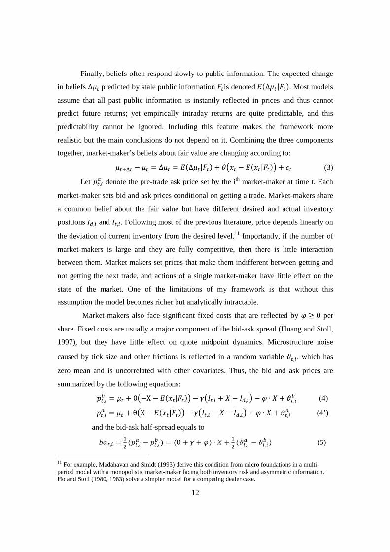
Finally, beliefs often respond slowly to public information. The expected change

in beliefs �� predicted by stale public information #�is denoted !���|#��. Most models

assume that all past public information is instantly reflected in prices and thus cannot

predict future returns; yet empirically intraday returns are quite predictable, and this

predictability cannot be ignored. Including this feature makes the framework more

realistic but the main conclusions do not depend on it. Combining the three components

together, market-maker’s beliefs about fair value are changing according to:

��'(� − �� = Δ�� = !�Δ��|#�� + �� � − !� �|#��$ + �� (3)

Let ��,*+ denote the pre-trade ask price set by the ith market-maker at time t. Each

market-maker sets bid and ask prices conditional on getting a trade. Market-makers share

a common belief about the fair value but have different desired and actual inventory

positions �,,* and ��,*. Following most of the previous literature, price depends linearly on

the deviation of current inventory from the desired level.11 Importantly, if the number of

market-makers is large and they are fully competitive, then there is little interaction

between them. Market makers set prices that make them indifferent between getting and

not getting the next trade, and actions of a single market-maker have little effect on the

state of the market. One of the limitations of my framework is that without this

assumption the model becomes richer but analytically intractable.

Market-makers also face significant fixed costs that are reflected by - ≥ 0 per

share. Fixed costs are usually a major component of the bid-ask spread (Huang and Stoll,

1997), but they have little effect on quote midpoint dynamics. Microstructure noise

caused by tick size and other frictions is reflected in a random variable .�,*, which has

zero mean and is uncorrelated with other covariates. Thus, the bid and ask prices are

summarized by the following equations:

��,*/ = �� + θ�−X − !� �|#��$ − 2���,* + 3 − �,,*$ − - ∙ 3 + .�,*

/ (4)

��,*+ = �� + θ�X − !� �|#��$ − 2���,* − 3 − �,,*$ + - ∙ 3 + .�,*

+ (4’)

and the bid-ask half-spread equals to

5��,* = 67

���,*+ − ��,*

/ � = �θ + 2 + -� ∙ 3 + 67

�.�,*+ − .�,*

/ � (5)

11 For example, Madahavan and Smidt (1993) derive this condition from micro foundations in a multi-period model with a monopolistic market-maker facing both inventory risk and asymmetric information. Ho and Stoll (1980, 1983) solve a simpler model for a competing dealer case.

13

Eq. (5) is a classic decomposition of the bid-ask spread into asymmetric

information θ, inventory risk 2 and fixed costs - components. Several methods are able

to separate fixed costs from the rest of the bid-ask spread, but the existing methods have

difficulty separating inventory and information components. Huang and Stoll (1997)

summarize this by saying that “estimates of adverse information probably include

inventory effects as well since existing procedures cannot distinguish the two.”12

Interestingly, Eq. (4) implies that if the difference between actual and desired inventory

levels is large, inventory risk will cause prices to deviate substantially from fair value

while having little effect on the bid-ask spread.

After following standard steps in Eq. (3-5), I explicitly account for the difference

in market-maker responses to trades. If t is time of a trade and Δ� is a small evaluation

period that gives market-makers just enough time to respond to it, market-makers will set

prices according to Eq. (4-5) at both times t and � + Δ�. However, how much the ask

price increases after a buyer-initiated trade differs for the trading and non-trading market

makers. To make it easier to follow, the analysis is first conducted only for a buy trade

and ask price and then is generalized at the end of this section. Section A.4 of the internet

appendix considers the case when trade direction is misclassified for some trades. The

trading market-maker gets extra inventory (X) and increases the ask price by

Δ��,*+ = !�Δ��|#�� + ��3 − !� �|#��$ + 2 ∙ 3 + ��'( + �.�'(�,*

+ − .�,*+ � (6)

while non-trading market-makers get the same information but no change in

inventory, thus they also increase ask price but by less than the trading market-maker:13

12 Those models that address this criticism sometimes produce counter-intuitive empirical results. For example, the method of Huang and Stoll (1997) relies on the autocorrelation in order flow to be negative. However, the autocorrelation is positive empirically which leads to negative estimates for the asymmetric-information component. Similarly, Hasbrouck (1988, 1991) suggests a vector-autoregressive framework that assumes that market-makers can relatively quickly restore their position to the desired level after an inventory shock. However, this assumption is often violated in practice as the lagged order flow in the autoregression usually covers only few minutes (about a hundred of one-second lags are common) while market-maker often spend many hours rebalancing inventory. 13 To better understand the multi-period price dynamics, consider an example of a sequence of buyer-initiated trades. Imagine, three market makers quote the same best ask price and three buy trades arrive one after another. After each trade, the trading market maker increases the ask price more than the non-trading peers. After the first trade, number of exchanges at the best asks decreases from three to two, and this number further shrinks to one after the second trade. But after the third trade, each market maker has received one trade and all three exchanges quote the best ask price again (the price will be higher of course because of inventory and information price impacts). This example illustrates how market makers maintain comparable inventory positions without direct interdealer trading.

14

Δ��,*8+ = !�Δ��|#�� + ��3 − !� �|#��$ + 2 ∙ 0 + ��'( + �.�'(�,*8

+ − .�,*8+ $ �6′�

To simplify the notation, assume that buy and sell trades are conditionally equally

likely, and thus !� �|#�� = 0; and that the noise/error terms are combined into a single

term ;�'(,< = ��'( + �.�'(�,*+ − .�,*

+ �, which has zero mean by construction. The price

responses of the trading (with index “i”) and non-trading (“i-“) market-makers in Eq. (6)

and (6’) can be then re-labeled with this simpler notation as:

Δ��,*+ = !�Δ��|#�� + �3 + 23 + ;�'(,< (7’)

��,*8+ = !���|#�� + �3 + ;�'(,<8 (7)

And the difference between the price responses for trading and non-trading

market-makers is:

Δ��,*+ − Δ��,*8

+ = 23 + �;�'(,< − ;�'(,<8� (8)

Price responses (7’) and (7) derived within this general framework match the

intuitive results of Eq. (1) in the previous section. Indeed, the price response of the

trading exchange (7’) contains both the inventory-risk and asymmetric-information

impacts, while the response of non-trading exchanges (7) contains only the information

impact �. However, both price responses also depend on the expected changes in price

!���|#�� and microstructure noise ;�. Microstructure noise ; has zero mean and thus

can be eliminated by taking an average over large number of trades. Note that the Law of

Large Numbers (LLN) requires that average instead of median should be taken; Section

A.3 explains that the distribution of ; is not symmetric due to price discreetness.

Unfortunately, the expected changes in price !��|#�� cannot be averaged out in

a similar way and should be estimated separately. Investors do not simply execute trades

at random – they time their trades (Hasbrouck, 1991). In particular, they buy when the

price is expected to increase anyway, and thus !��|#�� > 0 for buy trades and

!��|#�� < 0 for sell trades. Muravyev and Pearson (2014) further explain why

accounting for expected price changes is crucial.

The inventory-risk and asymmetric-information components of price impact can

be estimated from Eq. (7) and (8) in a sufficiently large sample so that the microstructure

noise terms are averaged to zero. Finally, it is time to generalize the formulas to account

for both buy and sell trades, which requires new notation. Trade direction indicator �*�? is

15

set to 1 for buy trades and -1 for sells. Price response ��,*�? is computed based on ask

prices for buys (��,*+ ) and based on bid prices for sell trades (��,*

/ ). After accounting for

this notation, the main equations for the price impact decomposition become as follows:14

Asymmetric information: � ∙ 3 = !@�*�? ∙ �Δ��,*8

�? − !�Δ��|#���A (9)

Inventory risk: 2 ∙ 3 = !@�*�? ∙ �Δ��,*

�? − Δ��,*8�? $A (10)

The inventory risk component of price impact is simply the difference between

price responses of trading and non-trading market-makers adjusted for trade direction.

The asymmetric information component is an average of price responses for non-trading

market-makers adjusted for the expected change in price due to slow diffusion of public

information. Again, the intuition of Eq. (2) is preserved in this general framework.

Finally, I outline how the main equations (9) and (10) can be applied to the data.

Section 4.3 implements this general outline for the options market. First, particular

methods for inferring trade direction ��? and expected price changes !���|#�� are

chosen. Standard algorithms (such as the quote rule) correctly classify the sign of vast

majority of trades. A regression model for expected quote changes is first estimated on

historical data and then the estimated model is applied to public information right before

a trade to produce the expected price change for this trade. Sections A.2 and A.4 of the

internet appendix further explain this step. Second, subset of all trades that satisfies

method assumptions is selected ({�} ⊂ �). I.e., trades with at least two exchanges quoting

the same best price in the direction of the trade; and these exchanges are used to compute

price responses for a given trade. Third, for each trade i in this subset (� ∈ {�}), I compute

the unexpected price change for non-trading exchanges �*�? ∙ �Δ��,*8

�? − !�Δ��|#��� and

the difference between price responses for the trading and non-trading exchanges

�*�? ∙ �Δ��,*

�? − Δ��,*8�? $ both of which are adjusted for trade sign �*

�?. Finally, Eq. (9) and

(10) imply that the average over all trades {�} for these individual trade responses

produces the final estimates of information and inventory price impacts.

3.3 Method’s assumptions and how they fit the optio n market

This section lists method’s assumptions and checks that the options market

satisfies them. The key assumptions include:

14 I.e., if ith trade is seller-initiated, its information price impact is computed as −�Δ��,*8

/ − !�Δ��|#���

16

1) Markets are transparent, and information is spread instantly. Information is

standardized: everybody receives the same message about a trade.

2) Liquidity is provided primarily by market makers. That is, most of the liquidity

providers are concerned about inventory risk.

3) Market makers do not actively share inventory directly with each other.

4) Many competitive market makers operate in the market.

5) Multiple market makers often quote the same best price.

Although a number of markets satisfy these assumptions, the equity options

market fits them particularly well. First, in early 2003 prior to the start of my sample

period, all options exchanges were connected through the Linkage, and the National Best

Bid and Offer (NBBO) rule was introduced. At the same time, investors got access to

real-time information about the best prices from all exchanges. In the age of floor-based

trading, market-makers on the exchange floor had better information about trades.15

However, this advantage diminished greatly in the modern electronic markets with

anonymous trade counterparties. Everybody gets a standard message with transaction

information in less than a second. All option market making is electronic, and the prices

are set by computer algorithms. The options market is at least as transparent and

technologically developed as the equity market.

Second, market makers stand on the liquidity-providing side of most trades.16 In

the options, market makers not only transfer liquidity in time but also across different

options. With more than a hundred option contracts available for each underlying, two

investors rarely select the same option; thus, they are likely to trade with a market maker.

Also, exchange rules grant lead market-makers substantial competitive edge over other

liquidity providers (e.g., the 60/40 NBBO order split rule17). These rules further

15 The method can be potentially applied even in a market where market makers have private information about the trades they receive. Other market makers can learn the information by observing the price response of the trading market maker and inferring the asymmetric information component from it. The mechanism is similar to Grossman and Stiglitz (1980) who show how uninformed traders learn the informed trader’s signal from the market equilibrium price in the fully revealing rational expectations equilibrium. 16 The Options Clearing Corporation (OCC) website has data on market maker versus other investor volume which confirm this point (http://www.theocc.com/webapps/onn-volume-search). 17 “Exchange Rule 6.76A: … When an LMM or DOMM is quoting on the book at the NBBO, the LMM or DOMM receives a guaranteed allocation of 40% of the incoming order ahead of any other non-Customer interest ranked earlier in time.” SEC Release No. 34-62598

17

strengthen the lead market-makers’ position as the main liquidity providers and make it

hard for new players to enter.

Third, market makers do not share inventory in the options market. This practice

was common in some OTC markets where dealers can trade directly with each other. For

example, Lyons (1997) shows evidence of “hot potato” trading in the FX market. A large

customer trade is followed by a sequence of smaller trades between dealers to share the

inventory. In this case, all dealers will get some inventory, and their price responses to a

trade will contain both information and inventory components. My method would

underestimate the inventory-risk and overestimate the asymmetric-information

component in this case. Section A.6 of the appendix shows that hot potato trading is not

common in the options market. Also, although a market-making firm often makes

markets in multiple stocks and at multiple exchanges, it makes market only at one

exchange for options on any given stock.

Fourth, the method requires that many fully competitive market-makers operate in

the market, otherwise the multi-period model becomes intractable. The strategic

interaction is limited if market-makers are fully competitive, because in this case they

post prices that make them indifferent between trading and not trading at any moment.

The prices are set conditional on getting a trade (Eq. 4) and thus do not depend on the

probability of getting it. That is, the quoted prices are the same irrespective of how many

exchanges are at the top of the book.18 Also, if competition is imperfect, market makers

will extract positive profits that are inversely proportional to the number of market-

makers at the top of the book in the oligopolistic-Cournot equilibrium (Kyle, 1989). If

three market-makers quote the same best ask price and a buy order arrives, two non-

trading market-makers will increase the price not only because of asymmetric

information but also because two market makers have more market power than three.

Thus, the method would underestimate the inventory-risk and overestimate the

asymmetric-information price impact in the case of imperfect competition. Empirically,

18 However, if the number of market-makers is small, the interaction shows up through the second order effect on the expected order flow. The price response of the trading exchange changes the state of the limit order book. The non-trading market makers will respond to this change because conditional on them getting the next trade, the expected time it takes for them to trade out of the extra inventory depends on the state of the book. The direction of this effect is unclear though. However, if there are many market makers, the effect is small because actions of a single market maker change the limit order book very little.

18

the competition is high in the options market, for most trades at least four exchanges

quote the best price. Also, instead of manually setting prices, market makers fully rely on

computer programs, making it harder to implement strategic interactions.

Firth, options exchanges quote the same price most of the time because of the

large tick size. For example, SEC report (2007, p. 8) shows that more than 75% of the

time at least three exchanges quote the same NBBO price. This number is consistent with

summary statistics for my sample in Table 1.

Finally, Section A.5 discusses empirical and theoretical implications of inferring

trade direction on my results. In short, because the method focuses on trades with

multiple exchanges quoting the trade price, my test design insures that the number of

misclassified trades is very small. Also, I show that trade misclassification does not

affect the relative magnitude but will make both components smaller, and thus make it

harder to find significant price impacts.

4. Data description and sample construction

4.1 Data description

The tick-level data were collected by Nanex, a firm specializing in selling real

time data feeds to proprietary traders. The dataset contains all quotes and trades for 39

stocks including four ETFs and their options from April 2003 to October 2006. The

selected stocks had the most liquid options based on option trading volume in March

2003. They consist of a number of stocks, e.g., large-capitalization technology stocks that

have persistently high option volume, along with a few smaller-capitalization stocks that

happened to be of trading interest during the spring of 2003. The data were archived and

time-stamped by Nanex to 25 millisecond precision as they arrived and come from all

U.S. exchanges where a given contract is traded. Nanex records the option part of the

data from OPRA data stream. The transaction price, size, exchange code, and some other

information are available for trades. OPRA does not report option trade direction, which

has to be inferred by applying the quote rule to the National Best Bid and Offer (NBBO).

If the trade is at the midpoint of the NBBO, the quote rule is applied to the best bid offer

(BBO) from the exchange at which the trade occurs. Section A.4 of the internet appendix

argues that this algorithm has small estimation error. The exchange-level best quotes and

volumes are available for quoted prices. That is, the data include each instance when any

19

exchange adjusts its best quote or quoted volume, even if this change does not alter

NBBO. The dataset also contains stock market data similar to TAQ. A more detailed

description of this dataset is provided by Muravyev, Pearson and Broussard (2013).19

For the daily-level analysis, the paper computes order imbalances with the data

obtained from the International Securities Exchange (ISE). The data set contains daily

non-market-maker volume for all options listed on ISE starting in May 2005. For each

option, the daily trading volume and number of trades have four types: open buy (close

buy), in which investors buy options to open new (close old) positions; open sell and

close sell. Trading volume is further divided by investor type, which allows me to

compute order imbalance faced by market-makers. The data only include transactions

which were executed at ISE; however, through most of the sample period, ISE was the

biggest equity options exchange with a market share of about 30%. OptionMetrics is a

common source of price information on equity options. For each option contract, it

contains end-of-day best bid and ask prices as well as other variables such as volume,

open interest, implied volatility, and option Greeks.20 Returns and volume for the

underlying stocks are also taken from OptionMetrics to avoid data loss from merging

with CRSP. After all filters, more than thousand stocks are in the final sample on each

day.

4.2 Data filters

The final sample, that satisfies the method requirements, is constructed in

multiple steps. First, a standard prescreening eliminates illiquid and bizarre options.

Trade transactions should satisfy the following conditions:

(a) An option should have time to expiration between 10 and 400 calendar days.

19 Some stocks dropped before the end of the sample period because of mergers (America Online, Calpine, Nextel, SBC) or ticker changes (Morgan Stanley, Nasdaq 100 ETF QQQ). The sample size for these stocks is relatively small which may lead to non-representative results. Two ETFs were included in the sample after the beginning. Initially, the method cannot be applied to Dow Jones ETF (DIA) because it was traded only at a single exchange, but it was added to the sample after other exchanges start trading its options. Nasdaq 100 ETF (QQQQ) changed a ticker and exchange listing; I report its results separately before and after the ticker change. 20 The implied volatility of an option is defined as the value of the volatility for the underlying stock which, when input in the Black–Scholes model will return an option price equal to the market price of this option. Implied volatility is often used as a substitute for option prices. Option Greeks are sensitivities of option price to changes in the underlying price and volatility.

20

(b) Option moneyness measured by absolute option delta (i.e., the sensitivity of

option price to changes in the underlying price) is between 0.2 and 0.8. That

is, options with at least some “optionality” are selected.

(c) The transaction time is between 9:35 and 15:55. The first and last 5 minutes of

trading are excluded to avoid open and close rotations.

Dropping any of these filters does not change the main results, and 15,298,816 out of

28,127,906 trade transactions satisfy these conditions.

The next step is to apply minimum conditions required by the method.

(d) At least two exchanges (including the one receiving a trade) quote the trade

price; otherwise, Eq. (10) is not well defined.

(e) Trade size is smaller than quoted size at the trading exchange. This condition

is set to avoid mechanical price impact at the trading exchange.

(f) Option bid price is larger than ten cents to avoid outliers as price impact is

normalized by option price.

Condition (d) also serves another purpose. Since trade price equals to the NBBO

price quoted by at least two exchanges, there is little ambiguity about trade direction as

further discussed in Section A.4. Condition (e) makes it less likely for the trading

exchange to move its quotes and if anything, work against finding a significant inventory-

risk impact. Conditions (d)-(f) further reduce the sample size to 7,684,944 trades. Finally,

few outliers with absolute price impacts of more than 50% are removed, which results in

a final sample of 7,684,040 trades. Thus, a significant portion of all option trades passes

all the filters. Panel B of Table 1 reports sample size at each screening stage.

4.3 Computation of price impact components

The information-risk and asymmetric-inventory price impacts are estimated by

applying Eq. (9) and (10) to the final sample of option trades that satisfy method’s

requirements from the previous section. I follow the general outline from the end of

Section 3.2. Specifically, each trade in the final sample is first processed independently

and then the average is taken for price responses over all trades. For each trade, I identify

non-trading exchanges that together with the trading exchange quote NBBO price in the

trade direction (price responses of the other exchanges are not used to avoid

endogeneity). These price responses are used to compute the price impact components in

21

four steps. First, following the method in Section A.2 of the internet appendix, I compute

the expected price changes: i.e., by how much the relevant quoted price (bid for sell

trades) were expected to change if no trade arrived. Second, following Eq. (9), the

information price impact is computed by subtracting the expected quote changes from the

actual quote changes for the non-trading exchanges over five-second evaluation period.

For example, if four exchanges (including the trading one) out of six quote NBBO price,

then the average is taken over the unexpected price responses of the three non-trading

exchanges. Third, following Eq. (10), the inventory price impact is computed as the

difference between the price responses for the trading and non-trading exchanges. Eq. (9)

and (10) also explicitly account for trade direction. The previous steps are computed in

dollar terms, the price impacts are then normalize by the option quote midpoint of a given

trade to make them comparable across options and stocks. Finally, as required by Eq. (9)

and (10), I take an average over all trades for these individual price impacts to compute

the final estimates of the asymmetric-information and inventory-risk components.

Summary statistics for the final sample are reported in Panel A of Table 1. The

asymmetric-information and inventory-risk impacts are 0.22% and 0.41% respectively.

Other sample statistics over the individual price impacts are also computed. The standard

deviation is larger for the inventory impact (1.6% versus 2.6%) because the information

impact averages price responses from multiple exchanges for each trade. The median

information impact is negative because due to large tick size, quoted prices do not change

after most trades while subtracted expected quote changes are mostly positive (quotes are

expected to move in the trade direction). This difference between the mean and median

caused by price discreetness is further explained in Section A.3 of the internet appendix.

On average, more than four exchanges out of six are quoting the best price at the

time of a trade. The distribution for trade size is close to exponential with a mean of 29

contracts (or about 3,700 dollars) and a median of 8 contracts (800 dollars). Consistent

with the literature on equity options, call trades outnumber put trades (66%); and there

are more seller-initiated trades (58%) but mostly in call options. Option and stock prices

vary substantially justifying why price impacts should be normalized.

22

5. Empirical results

The method produces five main empirical results. First, contrary to previous

literature (Vijh, 1990), I find that option trades have large price impact. The asymmetric-

information impact is 0.22% and the inventory risk impact is 0.41% for an average

trade.21 Thus, both asymmetric information and inventory risk are contributing

substantially to price formation. Table 2 shows that the asymmetric information

component is positive and significant for every stock in the sample. Except for two

special cases, America Online (0.02% in a small sample) and QQQ Nasdaq ETF (0.04%),

the remaining values are large and lie between 0.13% (Nextel) and 0.5% (Ford). The

price impacts remain positive for most subsamples of trades based on option and trade

characteristics.22

Second, inventory risk has larger price impact than asymmetric information for

every stock in my sample. Thus, option market-makers in my sample are more concerned

with managing inventory risk than with trading against an informed investor. Inventory

risk is of first-order importance and thus deserves more research attention. The inventory

impact is larger for any trade size and moneyness as shown in Figures 2 and 3. The

difference is particularly large for small trades and out-of-the-money options. The

inventory risk component is large for every stock in the sample: Dow Jones SPDR ETF

has the smallest impact of 0.19% while Bristol Myers - the highest of 1.0%.

Third, both price impacts are monotonically increasing in trade size. The

nonparametric estimates in Figure 2 show that the inventory impact is linear with some

concavity while the information impact is clearly concave. The result is formally

confirmed by a multivariate analysis in Tables 3 and A9 that accounts for both linear and

square root terms for trade size. The data supports square root as an appropriate

functional form here. The asymmetric-information impact for large orders (70 lots) is

about five times larger (0.1% vs. 0.5%) than for small orders (3 lots), while the increase

for the inventory impact is only twofold from 0.3% to 0.65%. The price impacts increase

21 Although not directly comparable, these numbers are also larger than typical price impacts in the stock market. Also, these price impacts are not only large in absolute value but also compared to typical abnormal option returns found in the option “anomalies” literature, which are typically less than 1% per day. 22 In untabulated results, I also confirm that both price impacts do not reverse at the time horizon of multiple minutes.

23

less steeply for very trades (more than hundred lots) resulting in a pronounced concavity

in this size region. Although, many theories predict that asymmetric-information impact

should be increasing in trade size, this result need to be reconciled with the results of

Anand and Chakravarty (2007) who find evidence of stealth trading in the options

market. More precisely, they find that Hasbrouck information share is twice as high for

mid-sized trades as for large trades (more than 99 contracts). There is little need for

stealth trading in the options market nowadays since order flow is sparse and is spread

across multiple contracts making it hard for informed traders to hide by splitting orders

into mid-sized pieces. A possible explanation is that Anand and Chakravarty (2007) use

data from 1999, when options were traded manually on the floor with no linkage between

exchanges.

Fourth, stock price instantly responds to option trades. This result confirms that

option trades indeed contain private information about the underlying price and

complements the existent literature, which is based mostly on daily return data. The

underlying price moves by 0.02 basis points (or 0.03 cents in dollar terms) in the

direction of option trade (after adjusting for option type; e.g., stock price decreases after

one buys a put). Although the effect is not large economically, it is highly statistically

significant and is positive for all but one stock (Nasdaq ETF QQQ). Last column in Table

3 reports how the stock price impact of option trades depends on option characteristics.

The single most significant variable is trade size. Large trades have three times more

impact than small trades. Surprisingly, trades of different moneyness have similar price

impact, while short-term options have slightly higher price impact. Overall, although

option trades contain significant information about the underlying price, most of their

information however is option-specific.

Tables 3 reports how the price impact components depend on option and trade

characteristics.23 Out-of-the-money options offer the highest leverage (exposure for a

dollar invested), and thus are particularly attractive for informed investors. Consistent

with this argument, the information price impact is decreasing and convex in absolute

23 Large sample size is necessary to estimate the price impacts because the distribution for quote changes is discrete and highly skewed with the majority of trades having zero impact. This discreetness is caused by a large tick size in the options market. R-square is low for the same reason. All regressions are estimated with stock-day (or stock) fixed effects, while kernel regression used for the figures are based on the pooled sample.

24

delta. Figure 3.D shows that the impact decreases from 0.4% for OTM options to 0.15%

for ITM options. Next, private information is often short-lived and is related to near-term

events, thus short-term options are better suited for informed investors in addition to

providing higher leverage. Indeed, the price impact decreases by 0.12% if time-to-

expiration decreases from 80 days to 20 days. Buyer-initiated trades have higher price

impact than sell trades because they give an opportunity to bet not only on future

volatility but also on the underlying direction. These results are broadly consistent with

Pan and Poteshman (2006), except that I do not find significant difference between call

and put options, perhaps because my sample consists of large stocks that are easy to sell

short. As for inventory risk, its price impact also decreases with moneyness from 0.8%

for OTM to 0.2% for ITM options. The put-call parity implies that the paired ITM and

OTM options should have similar risk profile, but because the price impact for OTM

options is normalized by smaller option price this mechanically leads to larger price

impact for them. Buy trades have much larger inventory impact (by 0.15%) because a

market-maker selling an option faces large downside risk. The inventory risk impact is

higher for calls than for puts because a seller of a call faces a risk of unlimited loses.

Overall, inventory and information impacts have similar conditional properties because

options with highest leverage also have highest inventory risk per dollar invested.

Several additional tests are reported in Table A9 and Figure 3. Earnings

announcement days are characterized by high intraday volatility and information

asymmetry. Indeed, both price impacts are higher on the announcement days. Time of

day has similar implications as volatility is high at the beginning and the end of trading.

Consistent with this hypothesis, both price impacts are higher during the first and last

hours of trading. Also, I find that the information impact increased significantly during

the sample period, while the inventory impact remained largely unchanged. To check the

robustness of nonparametric estimates of price impacts in Figure 2, I examine several

subsamples in Figure 3 and confirm that inventory risk continues to have bigger price

impact than asymmetric information for all of them. The first panel shows the price

impacts for the narrow range in absolute delta being between 0.4 and 0.6 and less than 50

days to expiration with the idea of checking the results within a homogenous set of

options. Next, I consider the sample with the number of quoting exchanges equal to three

25

instead of being at least two to check that the results are consistent if the number of

exchanges is fixed. Finally, the evaluation period is increased from 5 to 10 seconds in the

last subsample.

It should be repeated that because my sample consists mostly of stocks with liquid

options, the results are hard to extrapolate to stocks with illiquid options. To somewhat

address this concern, both information and inventory price impacts are larger for stocks

that had the lowest average option trading volume during the periods when they were in

the sample.24 Finally, my results offer little help in answering the puzzle of why option

bid-ask spreads are so huge. This is one of the biggest puzzles in the options literature;

the existing theories of option spread fail to explain its magnitude and shape (Muravyev

and Pearson, 2014). For example, the effective bid-ask spread is almost 7% of option

price in my sample of trades. I find that although inventory risk and asymmetric

information components are large, they explain only 18% of the spread size (and thus the

remaining 82% are attributed to fixed costs).25 These estimates are consistent with the

decompositions for the stock spread. For example, Huang and Stoll (1997) attribute

88.6% of the stock spread to the fixed costs component.

6. Inventory risk and daily option returns

The microstructure approach provides extensive evidence on the role of inventory

risk in option price formation. However, this approach is not suitable for answering some

of the questions. How large is the effect of inventory risk at the daily and longer

horizons? Inventory-risk effect is by definition temporarily; how long does it last? Also,

the tick-level options data are hard to process because of its large size, which constraints

the microstructure approaches to a small number of stocks (39 in my case). This section

introduces an independent approach to measuring inventory risk at the daily level, which

answers these questions and thus complements my intraday results.

After establishing the importance of inventory risk at the intraday level, this

section confirms this conclusion at the daily level with two pieces of evidence. First,

24 The five stocks with the lowest average daily option trading volume when they were in the sample were Capital One Financial, Calpine, Ford, SBC Communications, and Xilinx, with ticker symbols COF, CPN, F, SBC, and XLNX, respectively. 25 The share of the spread explained by the components can be computed as the sum of their magnitudes divided by bid-ask half spread, which is implied by Eq. (5). Specifically, 18% = (0.22%+0.4%)/3.46%.

26

using the full panel of option daily returns an instrumental variable estimation finds that

inventory-related part of option order imbalances has five times larger impact on option

prices than previously thought. Second, the order imbalances have more predictive power

than a set of fifty other plausible predictors of future option returns.

The literature shows the correlation between order imbalances and implied

volatility, while this paper complements it by identifying the inventory-related part of

order imbalance and quantifying its causal effect on option returns. More importantly, the

paper shows that inventory risk is not a secondary factor as previously thought but is a

primarily determinant of expected option returns. Bollen and Whaley (2004) are the first

to emphasize the importance of order flow for option prices. They show that daily

changes in the level and slope of implied volatility are positively correlated with the

same-day option order imbalance. Similarly, Garleanu et al. (2009) show that the market-

maker net positions are correlated with the spread between the observed implied volatility

and the implied volatility estimated from a jump-diffusion model.26 Although these

papers establish the importance of order flow, its magnitude is smaller than for other

determinants of option risk premium. Also, several issues complicate the interpretation of

their results.27 First, order flow is often informed, and thus prices can change in response

to information rather than inventory risk. Indeed, several papers (most notably Pan and

Poteshman, 2006) provide evidence of informed trading in the options market. The other

important concern is endogeneity. For example, both returns and order imbalances on a

given day are determined by common factors such as news. Are investors buying because

prices are rising or vice versa? This paper addresses these concerns by extracting

inventory-related component of order flow and using instrumental variable estimation to

account for endogeneity. After addressing these endogeneity concerns, the effect of

inventory risk on option prices is five times larger than previously thought.

6.1 Computation of option returns and order imbalan ces

The two key variables for the daily analysis are option returns and order

imbalances. Returns of delta-neutral option portfolios assess a cumulative risk premium

26 They also found a positive Sharpe ratio associated with net market-maker positions indicating that market makers are compensated for inventory risk. 27 Both of these papers are based predominantly on the pre-2000 data. The equity options market experienced a major change from floor-based to electronic trading after ISE entered the scene in May 2000.

27

embedded in option prices without relying on a specific option pricing model. Delta-

neutral portfolios are immune to small changes in the underlying and thus to stock risk

premiums. Order imbalance is a direct measure of changes in option market-maker

positions and thus their inventory risk. I divide options into four time-to-expiration

groups: expiring options (with less than 13 calendar days to expiration), short-term

options (with 30 days to expiration on average), mid-term options (with no more than 150

days left), and finally long-term options. For each day, stock and expiration group, I pick

the call-put pair closest to the at-the-money (ATM) point for the shortest expiration. For

the selected call-put pair, I compute option returns from the end of day t-1 until the end of

the next trading day t. Specifically, a straddle portfolio is created by buying one call

option and as many puts (�F��/|����| puts) as required to make it delta-neutral and

then this portfolio is hold for one day. Following the literature, I compute returns using

option quote midpoints. Eq. (11) summarizes the return definitions. For robustness, I also

use delta-neutral returns on individual calls. Unless otherwise stated, I refer to the delta-

neutral straddle returns for short-term options simply as “option returns”.

)t(W

)t(W)1t(WReturns;

)(

)( W:Straddle

t

ttt

−+=∆−

∆+= tt

tt P

P

CC (11)

Table 4 shows that average option returns are close to zero in my sample;

however, as expected, the return distribution is skewed and the median for daily returns is

-1.3%. If the underlying price does not change, straddle’s value decreases.

I compute option order imbalances accommodated by market-makers at the stock

level and then also aggregate them into the market-wide imbalance. Following Chordia

and Subrahmanyam (2004), order imbalance is defined as the difference between the

number of option buy and sell transactions by non-market-makers divided by the total

number of option trades on a given day. E.g., market-makers are net sellers of options if

the order imbalance is positive. Importantly, the data identifies which trade side is taken

by option market makers.

( )∑

∑ −=

iit,A,

iit,A,it,A,

tA, Trades#

SellTrades#BuyTrades#Imb Ord (12)

The simple order imbalance can be adjusted to distinguish between low and high

volume days by normalizing it by the average number of trades in the previous 30 days

28

instead of the number of trades on day t. A measure of market-wide order imbalance

shows whether option investors are buying or selling at the aggregate level. It is defined

as an average of individual order imbalances weighted by the average option volume

during the previous 250 trading days. Table 4 shows that option order imbalance is -5%

on average; option investors are net sellers of options (especially call options).

∑ ∑

==J

250

0 i-tJ,tJ,t OptVolume250

1*Imb Ord MWOrdImb

i (13)

After standard filters are applied,28 the final sample in most regressions exceeds

one million stock-day observations; with more than a thousand eligible stocks on a

typical day. The paper controls for most of the variables that are known to predict option

returns. The internet appendix describes more than 50 control variables. Tables 5 and A3

report summary statistics and correlations for selected variables. Interestingly, the

correlation table shows that despite option volume, skew and the bid-ask spread are often

used as proxies for demand pressure, they have a negligible correlation with the direct

measure of order imbalance.

6.2 Instrumental variables approach

An instrumental variables approach resolves the endogeneity between concurrent

option returns and order flow by establishing that past order imbalances are good

instruments of future imbalances. Past order imbalances predict future changes in market-

maker inventory, which in turn cause changes in option prices. This idea is implied by

Chordia and Subrahmanyam (2004) in their model.

The first stage of the 2-SLS regression establishes that option order imbalances

are highly persistent. In particular, future order imbalance is predicted separately by three

nested sets of instruments (Eq. 14). The first set contains only expiration day dummies,

with a separate dummy variable for each of five days centered on the post-expiration

Monday. The second instrument set expends the first set by adding two lags of market-

wide order imbalance to the expiration dummies. Market-wide imbalances are not

affected by informed trading as private information about the entire market is hard to

28 Stocks-days with stock prices below five dollars or with positive option volume on less than 80 days per year are excluded. Returns are computed only for options that satisfy three criteria: (1) both option bid prices should be larger than ten cents; (2) OptionMetrics deltas should be well defined; and (3) the option bid-ask spread should be less than 50% of the price and the quote midpoint should be larger than 40 cents.

29

obtain. Finally, the third set of instruments adds two lags of individual order imbalance to

the second set. With this instrument set, both time-series and cross-section dimensions

can be explored.

Expiration dummies are particularly good instruments. Investors substitute

expiring option positions with similar non-expiring ones in the three-day window around

the expiration day (every third Friday of a month). Because investors are short call and

put equity options on average, the rollover creates unprecedentedly large selling pressure

in the non-expiring options.29 Option expirations create exogenous variation in order

imbalance, and thus exogenous variation in market-maker inventories as investors open

new positions to replace positions in expiring options. Volatility and returns of the

underlying stocks change little around expiration; thus, fundamentals and informed

trading are not responsible for the order imbalance.

Lagged variables are a popular instrument choice in economics, and they indeed

solve the econometric problem here. However, it is not a priori clear whether all

predicted order imbalances should be attributed to the inventory-risk channel. For

example, individual order imbalances may be informed about future volatility and

through it, about future option returns. The private information contained in order

imbalances may take time to be reflected in the prices. Section A.9 in the internet

appendix addresses this concern by showing that the predicted order imbalances are

driven primarily by inventory risk rather than informed trading.

After settling on the instruments, I apply a standard 2-SLS approach to study the

effect of order imbalance on option returns, which is G6 in Eq. (14) and (15).

First stage:

}OrdImb,OrdImb ;{IVSet(2)IVSet(3)

}MWOrdImb,MWOrdImb ; {IVSet(1) IVSet(2)

n2}; n1, n0, n_1, n_2, { IVSet(1)

:sets instrument and {1,2,3} I where

εControls'IVSet(I)'AdjOrdImb

2,i-t1,i-t1-t1,i-t

2-t1-t1-t

t,i1,i-t1,i-t10t,i

==

=∈

+++= βββ

(14)

Second stage:

29 Lakonishok, Lee, Pearson, and Poteshman (2007) find that inventors (non-maker-makers) on average are short calls and puts on individual stocks.

30

t,i1,i-tt,i10t,i εControls'AdjOrdImbααOptRet +++= β (15)

All the coefficients in the first stage are highly significant as reported in Panel A

of Table 5, the instruments are strong. Order imbalance is extremely negative around

option expiration because investors are rolling over their positions to non-expiring

options. The selling pressure is particularly large on the post-expiration Monday when

the abnormal order imbalance riches -24%. Large negative order imbalances are also

observed on the day before and after (-8.7% and -11.7% respectively). The expiration

rollover is perhaps the strongest calendar seasonality in the options market. Next, order

imbalances are very persistent in the options market as both past market-wide and

individual imbalances have large positive coefficients. For example, a market-wide

imbalance of -10% today predicts a -6.5% imbalance tomorrow. Thus, if an option

market-maker observes an increase in his inventory on one day, then his net position is

likely continue to increase on the next day.

The second stage results are reported in Panel B of Table 5. First, the average

return sensitivity to order flow across the instrument sets is 0.15, which means that

inventory risk has a very large impact on option prices. For example, one standard

deviation increase in expected order imbalance (which is 25% for the last instrument set)

corresponds to 3.7% option return. Second, the OLS coefficient of 0.025 is consistent

with estimates by Bollen and Whaley (2004) after adjusting the units. However, this

coefficient is six times smaller than 0.15 produced by the instrumental variables

approach. Thus, accounting for endogeneity makes a big difference. The measurement

error bias can partially explain the difference in estimates.30 Third, the coefficient

estimates for all the instrument sets have similar magnitudes (15.4%, 17.8%, and 11.5%

respectively), which validates the instruments. Finally, the fact that market-wide order

imbalance has a significant effect on returns distinguishes the inventory channel from the

“mechanical price pressure” hypothesis. The price pressure hypothesis does not expect

option prices to be moved by order imbalance in other securities.

30 I show that the market-wide order imbalance is of central importance for option returns. If option returns are determined by market-wide order imbalance, but instead it’s substituted in the return regression by a noisy proxy such as individual order imbalance, then the coefficient will be biased. Indeed, individual imbalance is an unbiased estimate of the market-wide imbalance but has five times larger standard deviation which is large enough to cause a significant measurement error bias in a regression.

31

Overall, the instrumental variables approach shows that inventory risk is a major

factor for the entire panel of option daily returns.

6.3 Return predictability: inventory risk versus ot her factors

The instrumental variables approach assesses the absolute magnitude of the

inventory risk effect on option prices while this section evaluates its relative importance

for predicting future option returns. The instrumental variables approach shows that past

order imbalances are an excellent measure of future inventory shocks. Building on this

result, I conduct a first direct horse-race between the past order imbalance and more than

fifty of option returns predictors. The order imbalance wins the contest by a large margin.

Also, the horse-race ranks the relative importance of option “anomalies,” so that the

literature can focus on explaining the largest of them.

I estimate a panel regression in Eq. (16) where a set of past variables predict

option return on the next day. As suggested by the IV approach, individual and market-

wide order imbalances represent inventory risk. The internet appendix provides a

complete list of more than fifty control variables that include risk-neutral volatility,

implied skewness and kurtosis, past stock returns, different measures of stock volatility,

measures of size such as volume and capitalization, implied volatility skew and time

slope, and weekend dummy. These variables cover most of the known option market

“anomalies.” I test these variables in different combinations and select the best

combination containing about fifteen variables that avoids collinearity.

it,i1,-t1-t2i1,-t10it, εctorsOtherPredi'MWOrdImbαOrdImbααOptRet ++++= β (16)

Based on the results in Table 6, if the combined order imbalance increases by one

standard deviation, option returns are expected to be 1% higher on the next day, while

other predictors have a magnitude of at most 0.4% (per standard deviation). First, I

include the individual order imbalance on day t-1 which is highly significant with t-

statistics of 18 even in the presence of all the control variables. Next, I add the market-

wide order imbalance which has a t-statistic of “only” nine because its value is the same

for all stocks on a given day reducing its statistical power. To assess the combined

economic magnitude of order imbalance measures, I aggregate them into a single factor

using coefficient estimates from the regression.

32

Magnitudes of other predictors are mostly consistent with the literature and are

smaller than for the order imbalance. Out of fifty variables, the cross-section of option

return is most affected by absolute stock return (0.33% option return per standard

deviation increase) and the option bid-ask spread (0.2%). Christoffersen et al. (2011) find

similar magnitude for the spread. The fact that my results are consistent with other

theories reported in the literature indicates that my specification is reasonable. Weekend

return anomaly (introduced by Jones and Shemesh, 2012) is -1.3% on average, which

makes it perhaps the biggest calendar seasonality in option returns. Interestingly, during

my sample period, the weekend effect is mostly driven by the expiration weekend and

almost entirely disappears in the subsample of options with price above 2 dollars.

Changes and levels of implied volatility can predict next-day return (0.39%) but fail to

predict returns on subsequent days, and thus, are likely to be driven by microstruture

effects. Section A.10 of the internet appendix discusses these and other predictors and

their interpretation.

Overall, option order flow, a proxy for future inventory shocks, is by far the

strongest predictor of future option returns.

7. Conclusion

The paper presents three pieces of evidence that inventory risk has a primary

effect on option prices. First, I find that option trades have substantial price impact, and

the inventory-risk component of price impact is larger than the asymmetric-information

component for every stock in my sample. This intraday result is supplemented by two

results that use daily order imbalances accumulated by option market-makers. An

instrumental variable estimation finds that inventory-related part of option order

imbalances has five times larger impact on option prices than previously thought. Finally,

past order imbalances have more predictive power than a set of fifty other plausible

predictors of future option returns.

The daily results complement the intraday evidence in several ways. They show

that inventory risk has a long-term effect on option prices and provide alternative ways of

assessing its economic significance. For example, the inventory risk premium is larger

than most known option return “anomalies.” Also, these results show that inventory risk

33

matters for the full panel of optionable stocks and a longer sample period than is

available for the intraday analysis.

The paper introduces a novel method for decomposing the price impact of trades

into inventory-risk and asymmetric-information components and then applies it to the

equity options market. The inventory-risk component is inferred from the difference

between price responses of market-maker who receives a trade and those who do not. The

asymmetric-information component is estimated as an average price response by market-

makers who do not participate in a given trade adjusted for expected changes in price.

The method is particularly well suited for the options market; however, it can be also

applied to many other markets including the bond and equity markets. Overall, this

method contributes to the literature on the role and measurement of market maker

inventory risk and on distinguishing inventory from asymmetric information components

of bid-ask spreads.

I apply the method to equity options and find that inventory risk plays a primary

role in the option price formation. Both information and inventory price impacts are large

for option trades, but the inventory-risk component is almost always larger at least in my

sample. That is, option trades have high information content; however, although option

market-makers are concerned about trading against informed investors, they are even

more concerned with controlling inventory risk.

Overall, my results suggest that inventory risk in the options market, and

compensation for bearing it, are important components of option price dynamics.

34

Reference

Amihud, Yakov, and Haim Mendelson. "Dealership market: Market-making with inventory." Journal of Financial Economics 8.1 (1980): 31-53.

Anand, A. and S. Chakravarty. 2007. Stealth Trading in Options Markets. Journal of Financial and Quantitative Analysis 42, 167.

Bagnoli, Mark, S. Viswanathan, and Craig Holden. "On the existence of linear equilibria in models of market making." Mathematical Finance 11.1 (2001): 1-31.

Berkman, Henk. "Large option trades, market makers, and limit orders." Review of Financial Studies 9.3 (1996): 977-1002.

Bollen, N. P. B. and R. E. Whaley. 2004. Does Net Buying Pressure Affect the Shape of Implied Volatility Functions? The Journal of Finance 59, 711-753.

Boyle, Phelim P., and Ton Vorst. "Option replication in discrete time with transaction costs." The Journal of Finance 47.1 (1992): 271-293.

Cho, Young-Hye, and Robert F. Engle. “Modeling the impacts of market activity on bid-ask spreads in the option market.” No. w7331. NBER, (1999).

Choi, Jong Y., Dan Salandro, and Kuldeep Shastri. "On the estimation of bid-ask spreads: Theory and evidence." Journal of Financial and Quantitative Analysis 23.2 (1988): 219-230.

Easley, David, and Maureen O'Hara. "Price, trade size, and information in securities markets." Journal of Financial economics 19.1 (1987): 69-90.

Engle, Robert, and Breno Neri. “The impact of hedging costs on the bid and ask spread in the options market.” Working Paper, New York University, (2010).

Garleanu, N.; L. H. Pedersen and A. M. Poteshman. 2009. Demand-Based Option Pricing. Review of Financial Studies 22, 4259.

George, Thomas John, Gautam Kaul, and Mahendrarajah Nimalendran. "Estimation of the bid-ask spread and its components: A new approach." Review of Financial Studies 4.4 (1991): 623-656.

George, Thomas J., and Francis A. Longstaff. "Bid-ask spreads and trading activity in the S&P 100 index options market." Journal of Financial and Quantitative Analysis 28.3 (1993).

Glosten, Lawrence R., and Lawrence E. Harris. "Estimating the components of the bid/ask spread." Journal of financial Economics 21.1 (1988): 123-142.

Glosten, Lawrence R., and Paul R. Milgrom. "Bid, ask and transaction prices in a specialist market with heterogeneously informed traders." Journal of financial economics 14.1 (1985): 71-100.

Grossman, S. and J. Stiglitz, 1980, ‘On the impossibility of informationally efficient markets’, American Economic Review, 70, 393–408.

Harris, L.E., 1990. Estimation of stock price variances and serial covariances from discrete observations. Journal of Financial and Quantitative Analysis 25, 291Ð306.

Hasbrouck, Joel. "The summary informativeness of stock trades: An econometric analysis." Review of Financial Studies 4.3 (1991): 571-595.

Hasbrouck, Joel, and George Sofianos. "The trades of market makers: An empirical analysis of NYSE specialists." The Journal of Finance 48.5 (1993): 1565-1593.

Hendershott, T., S. Li, A. Menkvel, and M. Seasholes. 2013. Asset Price Dynamics with Limited Attention Hendershott, T. and M. S. Seasholes. 2007. Market Maker Inventories and Stock Prices. The American

Economic Review 97, 210-214. Ho, Thomas, and Richard G. Macris. "Dealer Bid-Ask Quotes and Transaction Prices: An Empirical Study

of Some AMEX Options." The Journal of Finance 39.1 (1984): 23-45. Ho, Thomas, and Hans R. Stoll. "On dealer markets under competition." The Journal of Finance 35.2

(1980): 259-267. Ho, Thomas, and Hans R. Stoll. "Optimal dealer pricing under transactions and return uncertainty." Journal

of Financial economics 9.1 (1981): 47-73. Ho, Thomas, and Hans R. Stoll. "The dynamics of dealer markets under competition." The Journal of

Finance 38.4 (1983): 1053-1074.

35

Huang, Roger D., and Hans R. Stoll. "The components of the bid-ask spread: A general approach." Review of Financial Studies 10.4 (1997): 995-1034.

Jameson, Mel, and William Wilhelm. "Market making in the options markets and the costs of discrete hedge rebalancing." The Journal of Finance 47.2 (1992): 765-779.

Kaul, Gautam, Mahendrarajah Nimalendran, and Donghang Zhang. "Informed trading and option spreads." Available at SSRN 547462 (2004).

Kavajecz, Kenneth A., and Elizabeth R. Odders-White. "An examination of changes in specialists' posted price schedules." Review of Financial Studies 14.3 (2001): 681-704.

Kyle, Albert S. "Continuous auctions and insider trading." Econometrica (1985): 1315-1335. Kyle, Albert S. "Informed speculation with imperfect competition." The Review of Economic Studies 56.3

(1989): 317-355. Lin, Ji-Chai, Gary C. Sanger, and G. Geoffrey Booth. "Trade size and components of the bid-ask spread."

Review of Financial Studies 8.4 (1995): 1153-1183. Lyons, Richard K. "A simultaneous trade model of the foreign exchange hot potato." Journal of

International Economics 42.3-4 (1997): 275-298. Madhavan, Ananth, and Seymour Smidt. "A Bayesian model of intraday specialist pricing." Journal of

Financial Economics 30.1 (1991): 99-134. Madhavan, Ananth, and Seymour Smidt. "An analysis of changes in specialist inventories and quotations."

The Journal of Finance 48.5 (1993): 1595-1628. Madhavan, A., M. Richardson, and M. Roomans. "Why do security prices change? A transaction-level

analysis of NYSE stocks." Review of Financial Studies 10.4 (1997): 1035-1064. Manaster, Steven, and Steven C. Mann. "Life in the pits: Competitive market making and inventory

control." Review of Financial Studies 9.3 (1996): 953-975. Mitchell, M.; L. H. Pedersen and T. Pulvino. 2007. Slow moving capital. Muravyev, Dmitriy, Neil D. Pearson, and John Paul Broussard, “Is there price discovery in equity

options?”, Journal of Financial Economics 107.2 (2013): 259-283. Muravyev, Dmitriy, and Neil D. Pearson (2014) “Option Trading Costs Are Lower Than You Think”

Working paper. Naik, Narayan Y., and Pradeep K. Yadav. "Do dealer firms manage inventory on a stock-by-stock or a

portfolio basis?" Journal of Financial Economics 69.2 (2003): 325-353. Pan, J. and A. M. Poteshman. 2006. The Information in Option Volume for Future Stock Prices. Review of

Financial Studies 19, 871. Securities and Exchange Commission. “Report Concerning Examinations of Options Order Routing and

Execution” (2007). Shachar, O., 2012. Exposing The Exposed: Intermediation Capacity in the Credit Default Swap Market.

Working paper. Stoll H. R. 1978, ‘The supply of dealer services in securities markets’, Journal of Finance, 33, 1133–51. Van Ness, Bonnie F., Robert A. Van Ness, and Richard S. Warr. "How well do adverse selection

components measure adverse selection?" Financial Management (2001): 77-98. Vijh, Anand M. "Liquidity of the CBOE equity options." The Journal of Finance 45.4 (1990). Wu, W.-S., Liu, Y.-J., Lee, Y.-T., Fok, R.C.W., Hedging costs, liquidity, and inventory management: The

evidence from option market makers. Journal of Financial Markets (2013).

36

Figure 1 A stylized example of how the asymmetric-information and inventory-risk components of price impact are computed for a buyer-initiated trade. Three market makers (A, C, and C) are quoting the same best ask price when a buy trade of size V* arrives to market maker A. Price responses are measured between time t and t+dt. Market maker A responds to both asymmetric information and change in inventory, while market makers B and C only react to trade information because their inventory do not change. For simplicity, this example assumes that the expected changes in the ask prices are zero.

Ask Price(t) Ask Price(t+dt)

Trade, V* Market Maker A

Market Maker B

Market Maker C

Information + Inventory Impacts

Price

Information Impact

Information Impact

37

Figure 2 Nonparametric estimates of the inventory-risk and asymmetric-information components of price impact as function of option trade size. The components of price impact are estimated by Eq. (9) and (10) and are measured over five-second evaluation period and are normalized by option quote midpoint. All price impacts and expected quote changes are adjusted to make the sign comparable across buys and sells. A kernel regression uses the Gaussian kernel with an adaptive width which is larger in the low-populated regions (big trade size). Each option contract is written on hundred underlying shares. Confidence intervals are not reported because they are trivial with large sample size.

38

Figure 3 Robustness checks for nonparametric estimates of inventory and information price impacts as function of trade size. The price impacts are computed according to Eq. (9) and (10). Panel A reports the price impacts for the subsample of trades that are at-the-money and have less than two months to expiration. Panel B shows the price impacts for trades with exactly three exchanges quoting the best price in the trade direction at the time of a trade. Panel C uses the evaluation period of ten seconds instead of five seconds for the main sample. Panel D reports how the price impacts depend on moneyness measured as absolute option delta. Option trade size is measured in contracts on hundred underlying shares each.

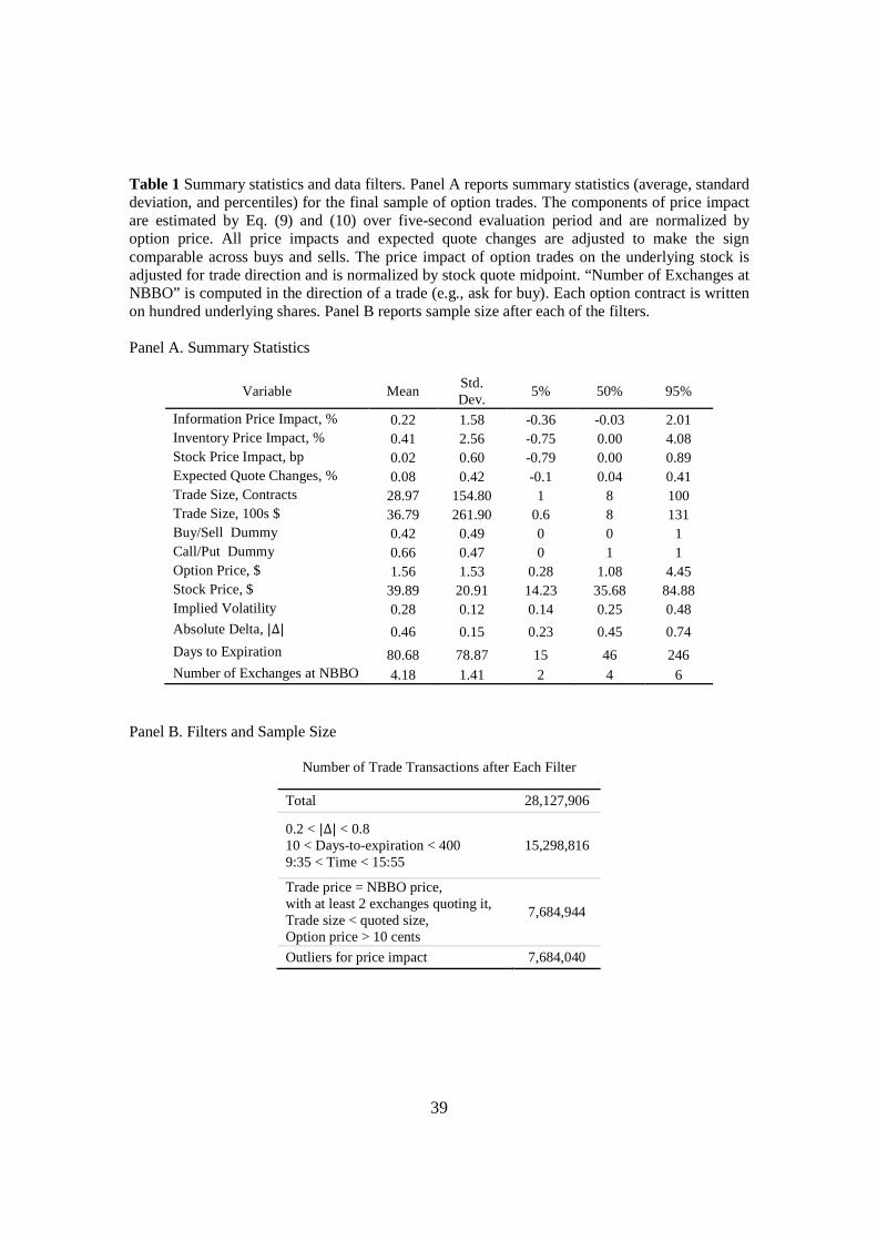
39

Table 1 Summary statistics and data filters. Panel A reports summary statistics (average, standard deviation, and percentiles) for the final sample of option trades. The components of price impact are estimated by Eq. (9) and (10) over five-second evaluation period and are normalized by option price. All price impacts and expected quote changes are adjusted to make the sign comparable across buys and sells. The price impact of option trades on the underlying stock is adjusted for trade direction and is normalized by stock quote midpoint. “Number of Exchanges at NBBO” is computed in the direction of a trade (e.g., ask for buy). Each option contract is written on hundred underlying shares. Panel B reports sample size after each of the filters. Panel A. Summary Statistics

Variable Mean Std. Dev.

5% 50% 95%

Information Price Impact, % 0.22 1.58 -0.36 -0.03 2.01 Inventory Price Impact, % 0.41 2.56 -0.75 0.00 4.08 Stock Price Impact, bp 0.02 0.60 -0.79 0.00 0.89 Expected Quote Changes, % 0.08 0.42 -0.1 0.04 0.41 Trade Size, Contracts 28.97 154.80 1 8 100 Trade Size, 100s $ 36.79 261.90 0.6 8 131 Buy/Sell Dummy 0.42 0.49 0 0 1 Call/Put Dummy 0.66 0.47 0 1 1 Option Price, $ 1.56 1.53 0.28 1.08 4.45 Stock Price, $ 39.89 20.91 14.23 35.68 84.88 Implied Volatility 0.28 0.12 0.14 0.25 0.48 Absolute Delta, |Δ| 0.46 0.15 0.23 0.45 0.74 Days to Expiration 80.68 78.87 15 46 246 Number of Exchanges at NBBO 4.18 1.41 2 4 6

Panel B. Filters and Sample Size

Number of Trade Transactions after Each Filter

Total 28,127,906

0.2 < |Δ| < 0.8 10 < Days-to-expiration < 400 9:35 < Time < 15:55

15,298,816

Trade price = NBBO price, with at least 2 exchanges quoting it, Trade size < quoted size, Option price > 10 cents

7,684,944

Outliers for price impact 7,684,040

Table 2 The components of price impact for the 36 stocks and 4 ETFs. Asymmetric information and inventory risk price impacts as well as expected changes in option price and the price impact of option trades on the underlying stock are reported for each stock in the sample. The components of price impact are estimated by Eq. (9) and (10). All price impacts and expected quote changes are adjusted to make the sign comparable across buys and sells. The averages in the last row are trade-weighted averages of the stock/ETF values. Ticker symbols indicated with * dropped before the end of the sample period (while ** were added after the start). ETFs are marked with “E”. All price impacts are reported in percent except for the stock price impact which is in basis points. Stock price impact is adjusted for trade direction (call/put, buy/sell) and is normalized by stock quote midpoint.

Stock # Obs. Infor-mation Impact

Inventory Impact

Expected Changes

Stock Price

Impact Stock # Obs.

Infor-mation Impact

Inventory Impact

Expected Changes

Stock Price

Impact AIG 116,845 0.21 0.28 0.07 0.024 IBM 250,684 0.14 0.23 0.08 0.011

AMAT 150,655 0.24 0.62 0.08 0.026 INTC 475,534 0.22 0.42 0.08 0.009 AMGN 180,918 0.20 0.31 0.10 0.028 JPM 148,222 0.25 0.43 0.07 0.014 AMR 94,975 0.36 0.52 0.06 0.061 KLAC 93,175 0.22 0.31 0.12 0.039

AMZN 217,455 0.21 0.31 0.10 0.054 MMM 91,807 0.20 0.28 0.07 0.020 AOL* 21,271 0.02 0.73 0.04 0.012 MO 181,345 0.18 0.27 0.06 0.012 BMY 82,125 0.34 1.00 0.06 0.011 MSFT 368,470 0.26 0.56 0.07 0.011

BRCM 175,646 0.22 0.28 0.09 0.053 MWD* 53,712 0.23 0.51 0.08 0.014 C 195,536 0.24 0.35 0.07 0.007 NXTL* 67,671 0.13 0.44 0.07 0.030

COF 58,791 0.21 0.35 0.07 0.043 ORCL 118,254 0.39 0.62 0.07 0.025 CPN* 50,278 0.44 0.73 0.05 0.044 PFE 289,798 0.28 0.51 0.07 0.005 CSCO 320,531 0.23 0.42 0.07 0.014 QCOM 256,123 0.22 0.25 0.11 0.036 DELL 185,196 0.28 0.37 0.09 0.025 QLGC 80,366 0.24 0.31 0.09 0.048

DIA** ,E 100,969 0.18 0.19 0.05 0.008 QQQ*,E 824,710 0.04 0.31 0.10 -0.003 EBAY 422,516 0.17 0.21 0.10 0.034 QQQQ**,E 678,154 0.26 0.55 0.13 0.006 EMC 106,407 0.31 0.74 0.06 0.016 SBC* 46,229 0.22 0.88 0.06 0.007

F 65,093 0.50 0.87 0.05 0.022 SMHE 162,516 0.23 0.40 0.08 0.022 GE 262,511 0.21 0.43 0.06 0.004 TYC 88,229 0.32 0.45 0.05 0.017 GM 199,507 0.31 0.44 0.07 0.027 XLNX 54,253 0.31 0.66 0.11 0.047 HD 147,018 0.18 0.40 0.06 0.011 XOM 200,545 0.19 0.44 0.06 0.013

Mean or

sum 7,684,040 0.22 0.41 0.08 0.018

Table 3 Price impacts conditional on trade and option characteristics. The components of price impact are estimated by Eq. (9) and (10). Nonlinearity in trade size is accounted for by including square root in addition to a linear term. Nonlinearity in absolute delta is accounted for by including variables equal to absolute delta for particular moneyness groups (OTM or ATM) and zero otherwise. Option trade size is measured in contracts on hundred underlying shares each. The absolute t-statistics reported in parentheses are based on robust standard errors clustered by date. Stock-date fixed effects are included but not reported.

Information Impact, %

Inventory Impact, %

Stock Price Impact, bp

Absolute Delta, |Δ| -0.746 -1.775 0.007

(22.25) (42.77) (1.52)

|Δ|, �� |Δ| < 0.4 -0.110 -0.347 0.001

(5.84) (13.04) (0.28)

|Δ|, �� 0.4 ≤ |Δ| < 0.6 -0.097 -0.227 -0.001

(12.64) (21.93) (0.35)

KDays to Expiration -0.027 -0.050 -0.001

(23.30) (40.54) (6.36)

Call/Put Dummy -0.000 0.073 -0.002

(0.05) (16.37) (2.85)

Option Price, $ 0.041 0.076 0.003

(17.36) (24.38) (5.72)

Buy/Sell Dummy 0.033 0.159 0.002

(5.44) (27.53) (2.72)

√Trade Size 0.032 0.018 0.005

(40.92) (21.68) (36.69)

Trade Size, Contracts -0.000 -0.000 -0.000

(16.57) (11.05) (2.84)

R2 0.04 0.03 0.01

# Obs. 7,684,040 7,684,040 7,684,040

42

Table 4. Summary statistics for daily data. Table reports mean, standard deviation, median as well as 10th and 90th percentiles for selected variables. Options are divided into four days-to-expiration groups. Ultra short-term (“p=0”) with less than 13 calendar days to expiration; short-term (“p=1”) with on average 30-days; mid-term (“p=2”) with no more than 150 days; and long-term (“p=3”) with more than 150 days. Option returns (“OptRet”) are computed for a delta-neutral straddle portfolio (long) based on the call-put pair which is closest to at-the-money. The order imbalance is based on the difference between the number of buy and sell trades normalized by the total number of trades on a given day (“OrdImb”) or by the average number of trades in the previous 30 days (“AdjOrdImb”). “MWOrdImb” is market-wide order imbalance. “OptBidAsk” is the dollar option bid-ask spread for short-term options. “OptVolume” is option volume measured in contracts. “IV30” is 30-days-to-expiration implied volatility. “Skew60” is a logarithm ratio of OTM to ATM implied volatilities for 60-days-to-expiration options. “RNSkewness” is risk-neutral skewness. “diff(IV)” is a one-day change in short-term implied volatility. “IV60 - StdRet” is the difference between implied and historical volatilities. Variables are based on the ISE open/close and OptionMetrics data. Complete variable definitions can be found in the internet appendix (Section B.1).

# Obs (in 1,000s)

Mean Std.Dev. P10% Median P90%

OptRet(p=0) 606 -0.010 0.505 -0.400 -0.059 0.431

OptRet, OptRet(p=1) 1,735 -0.000 0.096 -0.071 -0.013 0.077

OptRet(p=2) 1,819 0.000 0.051 -0.038 -0.004 0.041

OptRet(p=3) 1,817 0.001 0.033 -0.025 -0.001 0.028

OrdImb 1,813 -0.054 0.271 -0.400 -0.045 0.292

AdjOrdImb 1,813 -0.047 0.478 -0.442 -0.033 0.326

MWOrdImb 1,771 -0.058 0.045 -0.115 -0.057 -0.003

OptBidAsk, $ 1,805 0.196 0.225 0.050 0.150 0.350

OptVolumeUSD, $ 1,841 22340 293928 84 1421 26348

OptVolume, # 1,841 7295 48603 64 845 11917

IV30 1,841 0.444 0.221 0.218 0.400 0.723

diff(IV) 1,807 0.000 0.042 -0.034 -0.001 0.037

Skew60 1,841 0.109 0.108 0.018 0.098 0.208

RNSkewness 1,841 -0.600 0.432 -1.090 -0.559 -0.154

IV60 - IV360 1,841 0.025 0.070 -0.027 0.011 0.091

IV60-StdRet 1,841 -0.020 0.161 -0.165 0.004 0.100

StkRet 1,841 0.000 0.032 -0.032 0.000 0.032

AbsStkRet 1,841 0.021 0.024 0.002 0.014 0.047

StkPrice, $ 1,841 40.09 65.97 10.05 29.51 70.96

logME 1,825 21.99 1.66 20.00 21.84 24.14

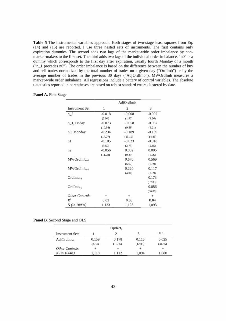
43

Table 5 The instrumental variables approach. Both stages of two-stage least squares from Eq. (14) and (15) are reported. I use three nested sets of instruments. The first contains only expiration dummies. The second adds two lags of the market-wide order imbalance by non-market-makers to the first set. The third adds two lags of the individual order imbalance. “n0” is a dummy which corresponds to the first day after expiration, usually fourth Monday of a month (“n_1 precedes n0”). The order imbalance is based on the difference between the number of buy and sell trades normalized by the total number of trades on a given day (“OrdImb”) or by the average number of trades in the previous 30 days (“AdjOrdImb”). MWOrdImb measures a market-wide order imbalance. All regressions include a battery of control variables. The absolute t-statistics reported in parentheses are based on robust standard errors clustered by date. Panel A. First Stage

AdjOrdImbt

Instrument Set: 1 2 3

n_2 -0.018 -0.008 -0.007

(3.94) (1.92) (1.86)

n_1, Friday -0.073 -0.058 -0.057

(10.94) (9.59) (9.21)

n0, Monday -0.234 -0.189 -0.189

(17.07) (15.19) (14.85)

n1 -0.105 -0.023 -0.018

(9.50) (2.73) (2.15)

n2 -0.056 0.002 0.005

(11.78) (0.29) (0.76)

MWOrdImbt-1 0.670 0.569

(6.67) (5.69)

MWOrdImbt-2 0.220 0.117

(4.00) (2.09)

OrdImbt-1 0.173

(37.03)

OrdImbt-2 0.086

(36.09)

Other Controls + + + R2 0.02 0.03 0.04 N (in 1000s) 1,133 1,128 1,093

Panel B. Second Stage and OLS

OptRett

Instrument Set: 1 2 3 OLS

AdjOrdImbt 0.159 0.178 0.115 0.025

(8.54) (10.36) (12.05) (31.56)

Other Controls + + + + N (in 1000s) 1,118 1,112 1,094 1,080

44

Table 6 Horse-race between option return predictors. Option returns on day t are predicted by order imbalances and other variables from day t-1. Column 2 reports standard deviations to facilitate computing economic magnitudes. Columns 3 and 4 gradually add order imbalances from day t-1. If two measures of order imbalance are combined into one factor weighted with estimated coefficients (0.008*OrdImbt-1+0.198* MWOrdImbt-1), this factor has standard deviation of 1%. Thus, one standard deviation change in the combined order imbalance changes expected returns on the next day by 1%. Short-term option returns are computed for a delta-neutral straddle portfolio (long) based on the call-put pair which is closest to at-the-money. The order imbalance is based on the difference between the number of buy and sell trades normalized by the total number of trades on a given day (“OrdImb”). MWOrdImb is a market-wide order imbalance. I also report the most significant control variables. “Weekend” dummy is one if t is Monday. “IV(p=1)” is implied volatility for short-term options. “diff(IV) t-1” is one-day change in short-term implied volatility. “AbsStkRett-1” is absolute stock returns. “COStdRet - StdRet” is open-close volatility relative to close-to-close volatility. The absolute t-statistics reported in parentheses are based on robust standard errors clustered by date.

Std. Dev.

OptRett OptRett

OrdImbt-1 0.27 0.012 0.008

(18.83) (16.12)

MWOrdImbt-1 0.04

0.198

(9.39)

Weekend 0.40 -0.013 -0.013

(4.20) (4.47)

OptRett-1 0.10 -0.027 -0.040

(4.23) (6.57)

diff(IV) t-1 0.04 -0.079 -0.088

(5.18) (5.87)

AbsStkRet t-1 0.02 0.142 0.165

(4.92) (5.94)

IV(p=1) t-1 0.23 -0.014 -0.016

(2.73) (3.04)

COStdRet -StdRet

0.03 -0.020 -0.025

(2.59) (3.33)

Other Controls

+ +

R 2

0.02 0.02

N (in 1000s)

1,161 1,161