Embed Size (px)
Citation preview
Organic and Conventional Vegetable Production in Oklahoma
Kalpana Khanal Dr. Francis M. EpplinResearch Assistant Professor Department of Agricultural Economics Department of Agricultural Economics Oklahoma State University Oklahoma State University421G Ag Hall 416 Ag HallPhone no. 405-744-9803 Phone no: 405-744-6156 Email: [email protected] Email: [email protected]
Dr. Shida Henneberry Dr. B. Warren RobertsProfessor Associate Professor Department of Agricultural Economics Oklahoma State UniversityOklahoma State University WWAREC424 Ag Hall 911 East Hwy 3, Lane, OK74555 Phone no.405-744-6178 Phone: 580-889-7343 Email: [email protected] Email: [email protected]
Dr. Merritt Taylor Dr. Jonathan Edelson Professor and Center Director Professor and Department HeadOklahoma State University Department of Entomology and Plant WWAREC Pathology911 East Hwy 3, Lane, OK 74555 Oklahoma State UniversityPhone: 580-889-7343 Email: [email protected]: [email protected]
Dr. R. Joe Schatzer Dr. Jim ShreflerProfessor Area Extension SpecialistDepartment of Agricultural Economics Oklahoma State UniversityOklahoma State University WWAREC420 Ag Hall 911 East Hwy 3, Lane, OK 74555 Phone: 405-744-6161 Phone: 580-889-7343 Email: [email protected] Email: [email protected]
Selected Paper prepared for presentation at the Southern Agricultural Economics Association Annual Meeting, Dallas, TX, February 2-6, 2008
Copyright 2008 by K. Khanal, S.R. Henneberry, M. Taylor, R.J. Schatzer, M. Epplin, B.W. Roberts, J. Edelson and J. Shrefler. All rights reserved. Readers may make verbatim copies of this document for non-commercial purposes by any means, provided that this copyright notice appears on all such copies.
Organic and Conventional Vegetable Production in Oklahoma
K. Khanal, S.R. Henneberry, M. Taylor, R.J. Schatzer, .M. Epplin, B.W. Roberts, J. Edelson, and J. Shrefler.
Abstract:
This study compares he profitability and risk related to conventional and organic
vegetable production systems A linear programming model was used to find the optimal mix of
vegetables in both production systems. And a target MOTAD (minimization of total absolute
deviation) model was used to perform risk analysis in both organic and conventional production
systems
2
ORGANIC AND CONVENTIONAL VEGETABLE PRODUCTION IN OKLAHOMA
INTRODUCTION
Background
The fruit and vegetable industry ranks fifth in U.S. agricultural exports and this sector
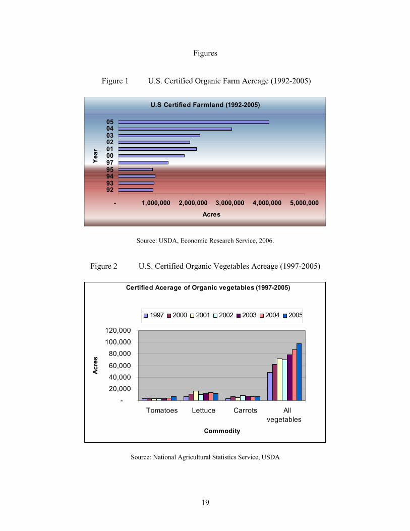
accounts for nearly a third of U.S. crop cash receipts (Lucier etal. 2006). As shown in figures 1
and 2 the total organic acreage as well as acreage of organic vegetables in the United States have
been increasing since the early 90’s.
Oklahoma farmers and ranchers are facing decisions concerning reduced government
support, increasing foreign competition, a changing demographic make-up of the domestic
population, and concentration of industry marketing power (Taylor, 2003). Many Oklahoma
farmers continue to examine alternative production and marketing strategies to enhance their
incomes. Horticultural crops may provide a niche for certain producers upon availability of
adequate resources and the required management skills. On the demand side consumers are
encouraged to increase their intake of fruits and vegetables. Despite the increasing demand and
potential profitability in this sector, studies related to economic feasibility of fruits and vegetable
production in Oklahoma have been limited to research conducted during the 1980’s and early
90’s.
Studies by Schatzer, Wickwire, and Tilley (1986) have shown that Oklahoma’s climatic
condition is favorable for horticultural industry as it has a relatively long growing season during
summer months, an abundance of good land, and a sufficient supply of waterIn this aspect Russo
and Taylor (2006) have stated that due to changes in demographics and economic hardships
faced by people, there is a growing interest in converting land to crops that are not traditional in
3
the southern plains of the U.S. and one such option in the southern plains is vegetable
production. Their study also states that in the southern plains like Oklahoma, land needs to be
taken out of row crops or cow-calf operations and make land available for the production of
vegetables.
Vegetables can be produced by both organic and conventional methods. The general
concept of organically grown produce refers to food that has not been treated with preservatives,
hormones or antibiotics and that has been grown without pesticides or artificial fertilizers in soil
whose humus content is increased by the addition of organic matter and whose mineral content is
increased by the application of natural mineral fertilizers. Data indicate that there were 40 acres
of certified organic vegetable production in Oklahoma in 2001 (USDA, 2002). Nevertheless, the
potential for organic vegetable production in Oklahoma is much beyond what is currently being
produced. An evaluation of the feasibility of the production of organic crops in Oklahoma would
assist the producers in choosing between organic productions versus the conventional
production.
This study focuses on calculating economic profitability of organic production in
Oklahoma and to compare it with economic profitability associated with vegetables produced
under conventional methods. Given their perishability, the level of risk associated with the
production and marketing of fresh vegetables is one of the major obstacles faced by Oklahoma
growers. Thus, risk analysis related to price and production issues is important for increasing the
number of growers in Oklahoma. More specifically; this study has focused on several selected
vegetables that constitute a large share of the value of vegetable production in Oklahoma. The
selected vegetables are tomatoes, watermelons, southern peas, sweet corn, pickling cucumber
and bell pepper.
4
Comparative Studies of Organic Versus Conventional Food
Estimates of the price variations between organic and conventional are commonly in the
range of 10-30 percent (Sok and Glaser, 2001). Still consumers are demanding more organic
foods, which show an increasing acceptance of organic agriculture in the United States.
Regarding the economic profitability of the U.S. organic crops, price premium is a key factor in
giving the organic farming systems comparable or higher whole farm profits. Armah (2002) also
has suggested the necessity of site-specific organic research. This study is expected to perform a
Southern Oklahoma based comparative study of conventional and organic vegetables. Sales of
organic food products have been increasing for the last ten years with sales of organic vegetables
increasing at a twenty percent rate per year for the last five years. It is perceived by many
consumers that organically produced vegetables are more tasty, healthier and safer than
conventionally grown vegetables. Because of this strong belief, the organic market is expected
to continue to expand. While the volume of the organic vegetable market is quite small relative
to that of conventionally produced vegetables, there appears to be opportunities for Oklahoma
growers to enter this niche market as a possible alternative to conventional production (Taylor,
Roberts, Edelson, Russo, Pair, Davis, Webber, 2006). Basic information on what is involved in
organic vegetable production such as required practices, acceptable varieties, costs of production
and expected returns are in limited availability. This study will attempt to answer many of the
questions regarding organic vegetable production.
Risk in Agricultural Production
The way risk is incorporated into production analysis varies among studies. Variability of
yields and prices should be considered in making crop choice decisions since uncertainty of yield
5
results from the unpredictable nature of the weather and performance of crops, whereas
uncertainty of prices comes from the market conditions (Anderson, Dillon and Harderker, 1977).
According to Taylor and Robinson (2004), the focus in risk management should be on reducing
the variability of income, not increasing net income.
Most risk-programming applications in agriculture are based on either mean-variance or
MOTAD (minimization of total absolute-deviations). MOTAD results are supposed to approach
mean variance results if returns are normally distributed. Also it is possible to consider
preference for risk even when decision variables are continuous and one way of doing that is to
apply a general version of MOTAD model referred to as the Target MOTAD model (McCamley
and Rudel, 1999).
As organic crop production increases this might lead to the reduction in price premium.
The reduced price premiums for organic products or lower profitability may discourage organic
farming. Thus, this study will help to disseminate information about profitability of organic
production system, under various risk scenarios compared to production under conventional
methods using Target MOTAD model.
PROCEDURES
Budgeting
6
To accomplish the first objective, enterprise budgets for selected vegetable enterprises are
developed for both organic and conventional systems. Budgets for watermelon, tomato, sweet
corn, determinate and indeterminate southern peas, pickling cucumber and bell pepper are
developed for three years 2004, 2005, 2006 for both organic and conventional systems; which
makes a total of forty-two budgets for this study. Each budget consists of variable costs, fixed
costs and expected revenues. The budgets are developed for the climatic and soil conditions of
Wes Watkins Agricultural Research and Extension Center at Lane, Oklahoma. All the budgets
are standardized so as to fix some exceptions and extremities. For example in one of the three
years tomato had to be replanted because of pest damage, but the replanting cost was not
included in that year’s tomato budget so that bias in results can be minimized. The costs in each
budget are average over three years and kept fixed in each year. Budgets from several states like
Oklahoma, Mississippi, Alabama, Arkansas etc. are refereed to for the standardization process.
These cost estimates are representative of average costs for farms in Southeastern
Oklahoma. Larger and smaller farms may have lower or higher costs per acre.
Price Data
In this study models were simulated using the same prices for both organic and
conventional produce, meaning profitability was calculated without a price premium in the
organic system. When prices were available from the Dallas Terminal Market these were
preferred. Producer received prices in Lane, Oklahoma were then extrapolated from the Dallas
terminal wholesale price data, assuming transportation and packaging cost margins of 30 percent.
The actual margin may vary by an unknown amount depending upon supply and the demand
7
situation in the Dallas Terminal Market (Wathen et al.). Price received in Lane is thus taken as
price in Dallas terminal market minus 30% of that price in Dallas Terminal Market.
Returns
Net returns of a farm enterprise are a function of the prices, quantities of inputs, and
outputs and costs. Return above operating costs (net return) is equal to the total revenue (yield
multiplied by price) minus total variable cost (summation of operating cost). Comparing returns
above operating cost of the different enterprises gives expected profitability of many of the
vegetable crops. Fixed costs are the same for all crops when produced by single crop.
The Linear Programming Model
A linear programming model for this study is designed to achieve the second objective of
the study which is to determine the profit maximizing vegetable mix for both organic and
conventional systems separately. The model is developed to maximize net returns for given
resource restrictions and farm organizations for both organic and conventional methods. A
matrix is developed to determine the optimal product mix for using different acreage and labor
wage rates. The rows consist of all the inputs that are constrained in the study. Each row is an
equation where the combined total of the resource levels used in a farm mix must be either
“equal to”, “less than” or “greater than” the constraint imposed, depending upon the type of
constraint. For example, one of the restrictions imposed is that no more than one third of the land
may be of tomato, pepper or the combination of the two. A similar restriction is imposed on
watermelon and cucumber. And, another on southern pea and sweet corn.
The columns consist of all of the production activities (organic and conventional
tomatoes, sweet corn, bell pepper, etc.), idle land, and balance rows for yields of production
8
activities for different years, non-labor cost balance, buying of labor from April to September
and Income balance for different years. Each parameter in the columns represents how many
units of the row resource are required for the particular column activity.
Twenty four different models were simulated to get the optimal values for different
combinations of land acreage, wage rate, and the type of labor used. The different acreages used
are: 6, 9 and 15; different wage rates used are: $10 and $15 per hour; and the two types of labor
used are: labor hired on a hourly basis and labor hired in a four month block. Only the results for
9 acres are included in this paper. The four months under block labor are: May, June, July, and
August and consists of 160 labor hours in one month.
The Target MOTAD Model
The target MOTAD model includes risk in a multi period approach and it fixes a static
target over several years. This model is designed to achieve the third objective of the study
which is a risk analysis of selected vegetables in both conventional and organic systems. It treats
the sample of variables as an empirical distribution and optimizes over the column space of the
sample. The results of the optimization are valid as long as the empirical distribution accurately
represents the true underlying distribution. Application of the Target MOTAD model requires
the decision maker to select a risk level for the expected deviation from an objective, and the
scientific basis for selecting a reasonable risk level (Qiu, Prato and McCamley, 2001).
The model is developed to determine the allocation of land and labor among the different
vegetables under the study including tomato, determinate southern pea, indeterminate southern
pea, sweet corn, watermelon, bell pepper, and pickling cucumber; such that net returns are
maximized, given the resource restriction in different farm conditions. Determinate southern
9
peas are harvested at one time, whereas, indeterminate southern peas have multi harvesting. So
labor cost involved with the later is higher. The Target MOTAD is constructed under the
assumption that the decision maker possesses the utility function )0,min( TRbaRcU −++= ,
where R is income, T is target income level, and a, b are parameters and are assumed to be
greater than zero (Tauer, 1983).
The Target MOTAD model was formed by setting a target on income constraint of the
simple programming model formed for objective two. Also λ (allowable average deviation below
the target income) was varied to trace out a risk return frontier. Since the Target MOTAD model
includes a linear objective function and linear constraints; the model was solved with a linear
programming algorithm using Excel Solver. The basic objective of the model is to analyze the
maximum expected return from the production of organic and conventional vegetables subject to
a given minimum level of risk identified with a predetermined target level of return. The target
income is the minimum income necessary to cover the fixed costs of farmers including credit
repayment, and to meet his family’s living costs each year.
RESULTS AND DISCUSSION
Linear Programming Model
A linear programming model is built from budgets and data sets specifying the objective
function, resource constraints, activity limits, and output prices. Excel Solver is used to
maximize the objective function. Linear Programming solution obtained by using the Excel
Solver is used to determine the profitability of hypothetical vegetable farms assuming three
production sizes of 6, 9, and 15 acres; and two wage rates10 and 15 dollars per hour hired labor
for both monthly hired labor and block labor. Results for 9 acres are included in this paper.
10
Altogether, eight different models were simulated for nine acres of land. Four scenarios
were formed using $10 per hour labor rate for monthly hired labor, for both organic and
conventional production methods. And four scenarios were simulated using $15 per hour labor
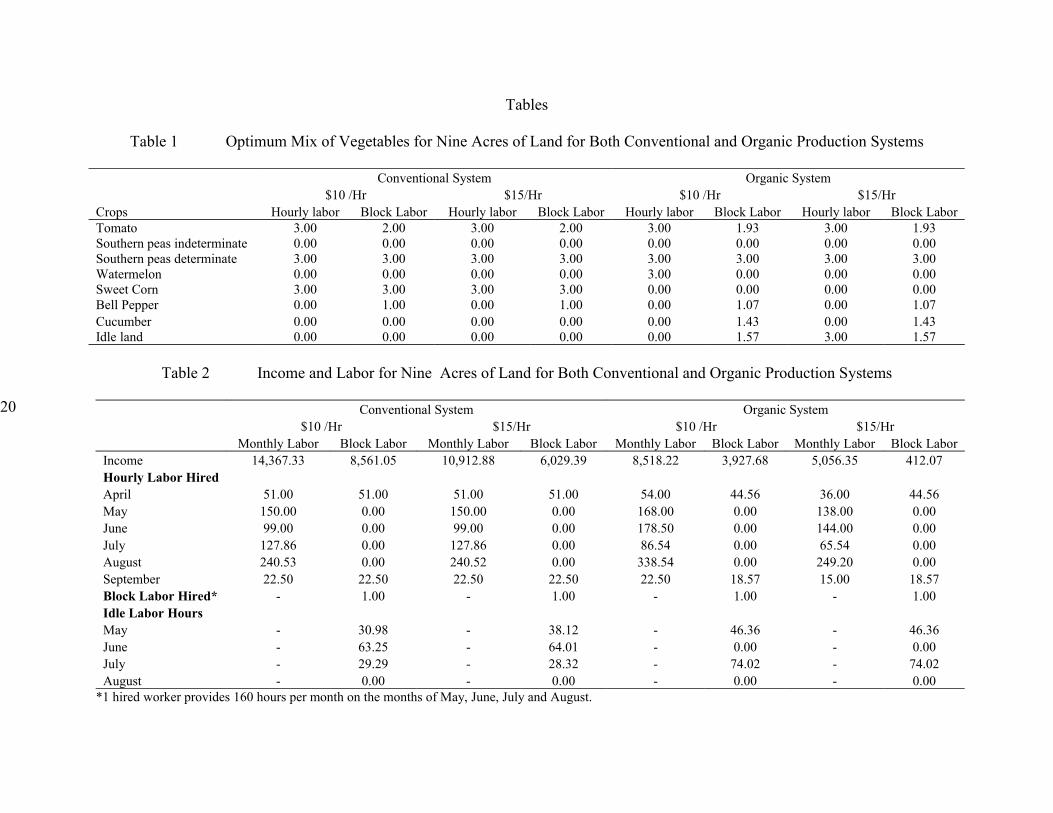
rate for block labor, for both organic and conventional systems. The results can be seen in tables
1 and 2. Assuming conventional methods using $10 for hourly labor, the optimal mix of
vegetables is: 3 acres of tomato, 3 acres of determinate southern peas, and 3 acres of sweet corn.
The optimal income for this situation is $14,367.33. For the same combination but assuming
organic method, the optimal mix of vegetable is: 3 acres of tomato, 2 acres of determinate
southern pea and 2 acres of watermelon and the optimal income is $8,518.22.
Assuming 10 dollars for block labor and the conventional system of production the
optimal mix of vegetables is: 2 acres of tomato, 3 acres of determinate southern peas, 3 acres of
sweet corn, and 1 acre of bell pepper, and the optimal income is $9,596.89. For the same
combination but assuming organic production system, the optimal income is $3,927.68 and the
optimal mix is: 1.93 acres tomato, 3 acres determinate southern peas, 1.07 acres bell pepper, 1.43
acres cucumber, and 1.57 acres idle land.
Likewise; using $15 for hourly labor for conventional system, the optimal mix of
vegetables is 3 acres of tomato, 3 acres of determinate southern peas, and 3 acres of sweet corn.
The optimal income for this case is $10,912.88. For the same combination in organic the optimal
income is $5,056.35 and the optimal vegetable mix is: 3 acres of tomato, 3 acres of determinate
southern peas, and 3 acres of idle land.
Whereas; using $15 for block labor for conventional system, the optimal vegetable mix
is: 2 acres of tomato, 3 acres of determinate southern peas, 3 acres of sweet corn, and 1 acre of
bell pepper. The optimal income is $6,029.39. For the same combination in organic, the optimal
11

income is $412.07 and the optimal vegetable mix is 1.93 acres of tomato, 3 acres of determinate
southern peas, 1.07 acres of bell pepper, 1.43 acres of cucumber, and 1.57 acres of idle land.
Exactly similar types of models were run for six and fifteen acres, the results for which
are not included in this paper.
Various scenarios are considered with varying assumptions about wage rates applied to
monthly hired labor and block labor. In scenarios including block labor, one of the column
restraints is the number of hired workers. Here this is constrained to be an integer. So in the
scenarios having block labor at least one worker has to be hired for the four months block. The
four months considered in the block are May, June, July and August. The results show that hiring
hourly labor is more profitable than hiring block labor for the same acreage, since labor hours
may remain idle when labor is hired in blocks causing a decrease in income.
Results show that for hourly labor, the optimal mix of vegetables were the same for
different acreage in conventional as well as organic but the number of acres for each crop
increased proportionately with the increase in total acreage. The most profitable mix of
vegetables for hourly labor in the conventional system are tomato, determinate southern pea and
sweet corn and that in organic system are tomato, determinate southern pea and watermelon. The
optimal mix for both conventional and organic system for block labor is different with a change
in acreage. In some cases when labor cost is $15, the organic system couldn’t pay the labor cost
and the results show that some acres of land are left idle.
Target MOTAD Model
The typical Target MOTAD model of vegetable farms under conventional and Organic
systems is constructed. Altogether four scenarios were applied to the Target MOTAD models to
12
perform the risk assessment for a vegetable farm. Two scenarios were developed for a 10 acre
conventional farm using block labor and monthly hired labor with labor rate of $10 per hour. On
the other hand, two additional scenarios assumed exactly the same combination of wage rate and
acreage in an organic system.
The objective function of the model is set to maximize expected net returns. The first set
of constraints imposes the resource restrictions. The second set of constraints defines deviations
below the target income in each time period. The third constraint sums the negative income
deviations times their probability of occurrence. This sum is represented by parameter λ and it is
interpreted as the expected deviation below target income. The models are solved by varying λ
from zero to a large number.
Risk Analysis Results for Conventional 9 Acres of Land
Assuming a conventional 9 acre farm and using block labor at the rate of $10 per hour,
the chosen target income is $8,200 dollars. Different farm plans were obtained by using the
Target MOTAD model changing the parameter λ which controlled the expected deviation below
target income. The λ values that were chosen are 0, 25, 50, 100 and 2,000. The expected incomes
for these λ values are $8296, $8420, $8492, $8635 and $9597 dollars. When the expected λ value
is equal to 2,000 it generates a solution which is equivalent to a linear programming solution.
The variation between higher and lower income has decreased with the decrease in λ and the
change in expected income is basically due to changes in acreage between tomato and bell
pepper which can be seen in table 3.
Whereas, assuming exactly the same farm scenario but using hourly labor at the rate of
$10 per hour, the chosen target income is $11,800. Also in this case, different farm plans were
13

obtained using target MOTAD model changing the parameter λ. The λ values in this case are
also 0, 25, 50, 100 and 2,000. The expected incomes for these λ values are $12,786, $13,532,
$14,264, $14,367 and $14,367. The expected value for λ equal to 100 and beyond is equivalent
to a linear programming solution in this case. These results are presented in table 4.
Risk Analysis Results for Organic 9 Acres of Land
Assuming an organic 9 acre farm and using hourly labor at the rate of $10 per hour the
chosen target income is $3,500. Different farm plans were obtained using the target MOTAD
model and changing the parameter λ which controlled the expected deviation below target
income. The λ values chosen for the organic system are same as that for conventional system.
The expected incomes for these λ values are $8235, $ 8303, $ 8320, $ 8353 and $ 8518. When
the expected value of λ is equal to 2000 the solution is equivalent to a linear programming
solution in this case.
The variation between higher and lower income has decreased slightly with the decrease
in λ but there is no major difference as in the conventional system. This may be due to the fact
that organic system is labor intensive, the farm income could not pay the cost involved when all
the available land resource was used. Thus, in most cases some of the land was left idle. Results
are presented in table 5.
Whereas, assuming exactly the same scenario but using four months block labor at the
rate of $10 per hour the chosen target income is $900. Different farm plans were developed using
the Target MOTAD model and changing the parameter λ which controlled the expected
deviation below target income. The λ values chosen are also 0, 25, 50, 100 and 2,000. The
expected incomes for these λ values are $2,539, $ 2,700, $ 2,861, $ 3,162 and $ 3,928 dollars.
14
When λ is set equal to 2,000 the expected value is equivalent to a linear programming
solution. Likewise, in this case the variation between higher and lower income has decreased
slightly with the decrease in λ, but there is no major difference as in the conventional system.
This may be due to the fact that organic system is labor intensive, the farm income could not pay
the cost involved when all the land resource was used. Thus, in most cases some of the land was
left idle. In this case acres for idle land are lower than that for the models ran with block labor. It
is one of the reasons for lower expected income as compared to results from model with hourly
labor. The existing variation in expected income is essentially due to changes in acreage among
bell pepper, cucumber and idle land. We can see significant changes in the acreage of idle land
with the change in λ values. These results can be seen in table 6.
The above solutions in all four cases are second-degree stochastic efficient as proved by
Tauer. In each table 3, 4, 5, and 6, five different farm plans can be seen. Some farm plans have
higher incomes, but higher variability between lower and higher incomes- whereas other farm
plans have lower incomes and lower variability between lower and higher incomes. It is up to the
farmers to choose the farm plan. The perception of the level of risk associated with an outcome
differs among decision makers. Furthermore, different farmers may have different attitudes
towards risk and therefore risk impacts can’t be assessed without accounting for the attitude of
the decision maker. But one important thing to be considered in decision making is the
variability between lower and higher incomes. The higher the variability, more risky is a farm
plan.
Required Price Premium to Grow Organic Vegetables
15
The results for objectives two and three are based upon using the same price for both
organic and conventional products. To determine the price premium necessary for the organic
products to breakeven with conventional production many simple programming models were
simulated for all the scenarios developed for organic system. The results can be seen in table 7.
The break even price premium ranges between 15% to 19%.
SUMMARY AND CONCLUSIONS
For this study seven different vegetable types were selected, namely determinate and
indeterminate southern pea, tomato, sweet corn, watermelon, pickling cucumber and bell pepper.
All of the selected vegetable budgets were incorporated into a programming model and an
optimal farm mix was determined for both Organic and Conventional systems. Based upon the
results, the mix of tomato, determinate southern peas and sweet corn is most profitable for the
conventional system and the mix of tomato, determinate southern pea and watermelon is most
profitable for the organic system. Block labor is more restrictive and less profitable compared to
the hourly labor.
The simple programming model formed was modified to a target MOATD model for risk
analysis. The risk analysis results show that higher variability existed in most of the cases in the
organic production system as compared to the conventional production system. In some cases, in
the organic system some acres of land were left idle due to higher production cost and higher risk
involved; whereas, all the acres were used in all cases in conventional production system.
Some simple programming models were also simulated to determine the break even price
premium in the organic system to get a similar optimum solution as in the conventional system.
The break even price premium ranged between 15-19%. Currently the price premium for organic
produce over the conventional ones still exists in most of the markets where consumers are
16

willing to pay higher prices for organic for various reasons. Therefore, in that case profitability
of organic production method can be seen as the function of price premium.
References
Anderson, J.R., J.L. Dillon, and J.B. Hardaker.1977. Agricultural Decision Analysis Ames: The Iowa State University Press
Armah, P.W. 2002. “Setting Eco-label Standards in the Fresh Organic Vegetable Markets of Northeast Arkansas.” Journal of Food Distribution Research 33(1): 35-45.
Lucier, G., S. Pollack, M. Ali, and A. Perez. 2006. U.S. Department of Agriculture, Economic Research Service, April.
http://www.ers.usda.gov/publications/VGS/apr06/vgs31301/vgs31301.pdf
McCamley,F. and R.K.Rudel.-1999. “Target MOTAD for Risk Lovers” Paper presented at Western Agricultural Economics Association Meeting, Fargo, ND, 11-14 July
Qiu, Z., T. Prato, and F. McCamley. 2001. “Evaluating Environmental Risks Using Safety-First Constraints” Americal Journal of Agricultural Economics 83(2):402-413.
Russo, V.M., and M.Taylor .2006. “Soil Amendments in Transition to Organic Vegetable Production with Comparison to Conventional Methods: Yields and Economics.” HortScience 41(7):1576-1583.
Schatzer, R.J., M.Wickwire, and D. Tilley.1986. “Supplemental Vegetable Enterprise for Cow-Calf and Grain Farmers in Southeastern Oklahoma.’’ Res. Re. No. T-874, Agr.Exp.Sta, Department of Agriculture Economics, Oklahoma State University.
Sok, E., and L. Glaser. 2001. “Tracking Wholesale Prices for Organic Produce,” Agricultural Outlook, U.S. Department of Agriculture, Economic Research Service, October, available at www.ers.usda.gov/publications/agoutlook/oct2001/ao285d.pdf
Tauer, Loren W. 1983. “Target MOTAD.” American Journal of Agricultural Economics 65:606-610.
Taylor, M.J. 2003.Oklahoma Agricultural Experiment Station Oklahoma State University, Hatch Project Proposal.
17
Taylor, M. J., J. R.C. Robinson.2004. “Risk Management for Investment in Vegetables”, Proceedings of Oklahoma-Arkansas Horticulture Industry Show, Tulsa, OK., January.
Taylor, M.J., W. Roberts, J.Edelson, V. Russo, S. Pair, A. Davis, C. Webber.2006. “Economic Evaluation of a Four (4) Crop Organic Vegetable Rotation”, Proceedings of the Bi-State Horticulture Industry Show, Tulsa, OK. January.
U. S. Department of Agriculture, Economic Research Service (USDA, ERS). 2002. Briefing Room-Organic Farming and Marketing: Questions and answers, June. www.usda.gov/nass
U.S. Department of Agriculture, Economic Research Service (USDA, ERS). 2006. “U.S.
Certified Farm Acreage 1992-2005”.
Wathen, B.L., M.J. Taylor, J.V. Edelson, B.W. Roberts, R.B. Holcomb. 2005. “Melon marketing and Price Volatility: Applied Study of the Southern Oklahoma Region.” Manuscript for Publication in the Journal of Agricultural and Applied Economics, February.
18
Figures
Figure 1 U.S. Certified Organic Farm Acreage (1992-2005)
U.S Certified Farmland (1992-2005)
- 1,000,000 2,000,000 3,000,000 4,000,000 5,000,000
9293949597000102030405
Year
Acres
Source: USDA, Economic Research Service, 2006.
Figure 2 U.S. Certified Organic Vegetables Acreage (1997-2005)
Certified Acerage of Organic vegetables (1997-2005)
-20,00040,00060,000
80,000100,000120,000
Tomatoes Lettuce Carrots Allvegetables
Commodity
Acre
s
1997 2000 2001 2002 2003 2004 2005
Source: National Agricultural Statistics Service, USDA
19
Tables
Table 1 Optimum Mix of Vegetables for Nine Acres of Land for Both Conventional and Organic Production Systems
Conventional System Organic System$10 /Hr $15/Hr $10 /Hr $15/Hr
Crops Hourly labor Block Labor Hourly labor Block Labor Hourly labor Block Labor Hourly labor Block LaborTomato 3.00 2.00 3.00 2.00 3.00 1.93 3.00 1.93Southern peas indeterminate 0.00 0.00 0.00 0.00 0.00 0.00 0.00 0.00Southern peas determinate 3.00 3.00 3.00 3.00 3.00 3.00 3.00 3.00Watermelon 0.00 0.00 0.00 0.00 3.00 0.00 0.00 0.00Sweet Corn 3.00 3.00 3.00 3.00 0.00 0.00 0.00 0.00Bell Pepper 0.00 1.00 0.00 1.00 0.00 1.07 0.00 1.07Cucumber 0.00 0.00 0.00 0.00 0.00 1.43 0.00 1.43Idle land 0.00 0.00 0.00 0.00 0.00 1.57 3.00 1.57
Table 2 Income and Labor for Nine Acres of Land for Both Conventional and Organic Production Systems
Conventional System Organic System$10 /Hr $15/Hr $10 /Hr $15/Hr
Monthly Labor Block Labor Monthly Labor Block Labor Monthly Labor Block Labor Monthly Labor Block LaborIncome 14,367.33 8,561.05 10,912.88 6,029.39 8,518.22 3,927.68 5,056.35 412.07Hourly Labor HiredApril 51.00 51.00 51.00 51.00 54.00 44.56 36.00 44.56May 150.00 0.00 150.00 0.00 168.00 0.00 138.00 0.00June 99.00 0.00 99.00 0.00 178.50 0.00 144.00 0.00July 127.86 0.00 127.86 0.00 86.54 0.00 65.54 0.00August 240.53 0.00 240.52 0.00 338.54 0.00 249.20 0.00September 22.50 22.50 22.50 22.50 22.50 18.57 15.00 18.57Block Labor Hired* - 1.00 - 1.00 - 1.00 - 1.00Idle Labor HoursMay - 30.98 - 38.12 - 46.36 - 46.36June - 63.25 - 64.01 - 0.00 - 0.00July - 29.29 - 28.32 - 74.02 - 74.02August - 0.00 - 0.00 - 0.00 - 0.00
*1 hired worker provides 160 hours per month on the months of May, June, July and August.
20

Table 3 Risk Analysis For Conventional 9 Acres of Land Using Block Labor for $10 an Hour
Target Income Average deviation Expected Income High Income Low Income Tomato SP-Det Sweet Corn Bell pepper$8,200 0 $8,296 $8,646 $8,200 2.29 3.00 3.00 0.71$8,200 25 $8,420 $8,936 $8,125 2.28 3.00 3.00 0.72$8,200 50 $8,492 $9,226 $8,050 2.26 3.00 3.00 0.74$8,200 100 $8,635 $9,805 $7,900 2.23 3.00 3.00 0.77$8,200 2,000 $9,597 $13,312 $6,842 2.00 3.00 3.00 1.00
Table 4 Risk Analysis for Conventional 9 Acres of Land Using Hourly Labor for $10 an Hour
Target Income Average deviation Expected Income High Income Low Income Tomato SP-Det Sweet Corn Watermelon SP-Indet$11,800 0 $12,786 $14,759 $11,800 3.00 2.83 3.00 0.17 0.00$11,800 25 $13,532 $17,070 $11,725 3.00 2.86 3.00 0.14 0.00$11,800 50 $14,264 $19,343 $11,650 3.00 2.89 3.00 0.05 0.06$11,800 100 $14,367 $19,455 $11,629 3.00 3.00 3.00 0.00 0.00$11,800 2,000 $14,367 $19,455 $11,629 3.00 3.00 3.00 0.00 0.00
Table 5 Risk Analysis for Organic 9 Acres of Land Using Hourly Labor for $10 an Hour
Target Income Average deviation Expected Income High Income Low Income Tomato SP-Det Watermelon Idle Land$3,500 0 $8,235 $12,494 $3,500 3.00 2.88 0 3.12$3,500 25 $8,303 $12,536 $3,425 3.00 3.00 0.10 2.90$3,500 50 $8,320 $12,537 $3,350 3.00 3.00 0.33 2.67$3,500 100 $8,353 $12,540 $3,200 3.00 3.00 0.78 2.22$3,500 2,000 $8,518 $12,552 $2,462 3.00 3.00 3.00 0.00
21

Table 6 Risk Analysis for Organic 9 Acres of Land Using Block Labor for $10 an Hour
Target Income Average deviation Expected Income High Income Low Income Tomato SP-Det Bell Pepper Cucumber Idle land$900 0 $2,539 $5,818 $900 2.19 3.00 0.81 1.28 1.72$900 25 $2,700 $6,376 $825 2.16 3.00 0.84 1.29 1.71$900 50 $2,861 $6,934 $750 2.13 3.00 0.87 1.31 1.69$900 100 $3,162 $6,997 $600 2.08 3.00 0.92 1.34 1.66$900 2,000 $3,928 $6,133 $209 1.93 3.00 1.07 1.43 1.57
Table 7 Break Even Price Premium in Organic System to Obtain Same Level of Optimal Solution as in Conventional.
Hourly labor Block Labor$10 /Hr $15/Hr $10 /Hr $15/Hr
Income Price Premium Income Price Premium Income Price Premium Income Price Premium6 Acres 9,816.90 15% 7,324.90 17% 7,310.54 17% 4,546.54 17%9 Acres 14,725.35 15% 10,987.34 17% 9,618.99 19% 6,103.37 19%15 Acres 24,542.25 15% 18,312.24 17% 17,300.43 18% 10,172.03 18%22