Organizational Barriers to Technology Adoption:

Evidence from Soccer-Ball Producers in Pakistan∗

David Atkin†, Azam Chaudhry‡, Shamyla Chaudry§,

Amit K. Khandelwal¶ and Eric Verhoogen‖

First Draft: December 2013

This Draft: July 2014

Abstract

This paper studies technology adoption in a cluster of soccer-ball producers in Sialkot,

Pakistan. Our research team invented a new cutting technology that reduces waste of the

primary raw material. We allocated the technology to a random subset of producers. Despite

the arguably unambiguous net benefits of the technology for nearly all firms, after 15 months

take-up remained puzzlingly low. We hypothesize that an important reason for the lack

of adoption is a misalignment of incentives within firms: the key employees (cutters and

printers) are typically paid piece rates, with no incentive to reduce waste, and the new

technology slows them down, at least initially. Fearing reductions in their effective wage,

employees resist adoption in various ways, including by misinforming owners about the value

of the technology. To investigate this hypothesis, we implemented a second experiment

among the firms to which we originally gave the technology: we offered one cutter and one

printer per firm a lump-sum payment, approximately equal to a monthly wage, that was

conditional on them demonstrating competence in using the technology in the presence of

the owner. This incentive payment, small from the point of view of the firm, had a significant

positive effect on adoption. We interpret the results as supportive of the hypothesis that

misalignment of incentives within firms is an important barrier to technology adoption in

our setting.

∗We are grateful to the International Growth Centre for generous research support; to Tariq Raza, AbdulRehman Khan, Fatima Aqeel, Sabyasachi Das and Daniel Rappoport for excellent research assistance; to ResearchConsultants (RCONS), our local survey firm, for tireless work in carrying out the surveys; and to Esther Duflo,Florian Ederer, Cecilia Fieler, Dean Karlan, Asim Khwaja, Rocco Macchiavello, David McKenzie, Ben Olken,Ralph Ossa, Anja Sautmann, Chris Udry, Reed Walker and several seminar audiences for helpful discussions. Weare particularly grateful to Annalisa Guzzini, who shares credit for the invention of the new technology describedin the text, and to Naved Hamid, who first suggested we study the soccer-ball sector in Sialkot. All errors areours.†Yale University, Dept. of Economics. E-mail: david.atkin@yale.edu‡Lahore School of Economics. E-mail: azam@lahoreschool.edu.pk§Lahore School of Economics. E-mail: shamyla@lahoreschool.edu.pk¶Columbia Graduate School of Business. E-mail: ak2796@columbia.edu‖Columbia University, Dept. of Economics and SIPA. E-mail: eric.verhoogen@columbia.edu

1

1 Introduction

Observers of the process of technological diffusion have been struck by how slow it is for many

technologies.1 A number of the best-known studies have focused on agriculture or medicine,2 but

diffusion has also been observed to be slow among large firms in manufacturing. In a classic study

of major industrial technologies, for instance, Edwin Mansfield found that it took more than 10

years for half of major U.S. iron and steel firms to adopt by-product coke ovens or continuous

annealing lines.3 More recently, Bloom, Eifert, Mahajan, McKenzie, and Roberts (2013) found

that many Indian textile firms are not using standard (and apparently cheap to implement)

management practices that have diffused widely elsewhere. The surveys by Stoneman (2002),

Hall and Khan (2003) and Hall (2005) contain many more examples.

Why is adoption so slow for so many technologies? The question is key to understanding

the process of economic development and growth. It is also a difficult one to study, especially

among manufacturing firms (Tybout, 2000). It is rare to be able to observe firms’ technology

use directly, and rarer still to have direct measures of the costs and benefits of adoption, or

of what information firms have about a given technology. As a consequence, it is difficult to

distinguish between various possible explanations for low adoption rates.

In this paper, we present evidence from a cluster of soccer-ball producers in Sialkot, Pakistan,

that a conflict of interest between employees and owners within firms is an important barrier

to adoption. The cluster produces 30 million soccer balls a year, or about 40 percent of world

production, including match balls for the 2014 World Cup, and about 70 percent of world hand-

stitched production (Wright, 2010; Houreld, 2014). The setting has two main advantages for

understanding the adoption process. The first is that the industry is populated by a substantial

number of firms — 135 by our initial count — producing a relatively standardized product and

using largely the same, simple production process. The technology we focus on is applicable at

a large enough number of firms to conduct statistical inference.

The second, and perhaps more important, advantage is that our research team, through a

series of fortuitous events, discovered a useful innovation: we invented a new technology that

represents, we argue, an unambiguous increase in technical efficiency for nearly all firms in the

sector. The most common soccer-ball design combines 20 hexagonal and 12 pentagonal panels

(see Figure 1). The panels are cut from rectangular sheets of an artificial leather called rexine,

typically by bringing a hydraulic press down on a hand-held metal die. Our new technology,

described in more detail below, is a die that increases the number of pentagons that can be cut

1For instance, in a well-cited review article, Geroski (2000) writes: “The central feature of most discussionsof technology diffusion is the apparently slow speed at which firms adopt new technologies” (p. 604). See alsoRosenberg (1982).

2See, for instance, Ryan and Gross (1943), Griliches (1957), Coleman and Menzel (1966), Foster and Rosen-zweig (1995), and Conley and Udry (2010).

3See Mansfield (1961) and the summary in Table 2 of Mansfield (1989).

2

from a rectangular sheet, by implementing the best packing of pentagons in a plane known to

mathematicians. A conservative estimate is that the new die reduces rexine costs for pentagons

by 6.25 percent and reduces total costs by approximately 1 percent — a modest reduction but

not an insignificant one in an industry where mean profit margins are 8 percent. The new

die requires minimal adjustments to other aspects of the production process. Importantly, we

observe adoption of the new die very accurately, in contrast to studies that infer technology

adoption from changes in residual-based measures of productivity such as those reviewed in

Syverson (2011).

We randomly allocated the new technology to a subset of 35 firms (which we refer to as the

“tech drop” group) in May 2012. To a second group of 18 firms (the “cash drop” group) we

gave cash equal to the value of the new die (US$300), and to a third group of 79 firms (the “no

drop” group) we gave nothing. We initially expected the technology to be adopted quickly by

the tech-drop firms, and we planned to focus on spillovers to the cash-drop and no-drop firms

and the channels through which they operate; we pursue this line of inquiry in a companion

paper (Atkin, Chaudhry, Chaudry, Khandelwal, and Verhoogen, 2014). In the first 15 months

of the experiment, however, the most striking fact was how few firms had adopted, even among

the tech-drop group. As of August 2013, five firms from the tech-drop group and one from the

no-drop group had used the new die to produce more than 1,000 balls in the previous month, our

preferred measure of adoption. The experiences of the adopters indicated that the technology

was working as expected; we were reassured, for instance, by the fact that the one no-drop

adopter was one of the largest firms in the cluster, and had purchased a total of 32 dies on 9

separate occasions. Overall, however, adoption remained puzzlingly low.

In our April 2013 survey round, we asked non-adopters in the tech-drop group why they

had not adopted. Of a large number of possible responses, the leading answer was resistance

from cutters. Anecdotal evidence from a number of firms we visited suggested that workers were

resisting the new die, including by misinforming owners about the productivity benefit of the

die. We also noticed that the large adopter (purchaser of the 32 dies) differed from the norm

for other firms in its pay scheme: while more than 90 percent of firms pay a pure piece rate, it

pays a fixed monthly salary plus a performance bonus.

The qualitative evidence led us to hypothesize that a misalignment of incentives within the

firm is an important reason for the lack of adoption. The new die slows cutters down, certainly

in the initial period when they are learning how to use it, and possibly in the longer run

(although our data suggest that the long-run speed is nearly the same as for the existing die).

If cutters are paid a pure piece rate, their effective wage will fall in the short run. The new die

requires a slight modification to another stage of production, printing, and printers face a similar

but weaker disincentive to adopt. Unless owners modify the payment scheme, the benefits of

using the new technology accrue to owners and the costs are borne by the cutters and printers.

3

Realizing this, the workers resist adoption. We formalize this intuition in a simple model of

strategic communication between an imperfectly informed principal and a perfectly informed

agent within a firm. When standard piece-rate contracts are used, there is an equilibrium

in which the agent misinforms the principal about the benefits of the new technology and the

principal is influenced by the agent not to adopt it. A relatively simple modification to the labor

contract, conditioning the wage contract on marginal cost, an ex-post-revealed characteristic of

the technology, induces the agent to truthfully reveal the technology and the principal to adopt

it.

To investigate the misalignment-of-incentives hypothesis, we designed and implemented a

new experiment. In September 2013, we randomly divided the set of 31 tech-drop firms that

were still in business into two groups, a treatment group (which we call the A group) and a

control group (the B group).4 To the B group, we simply gave a reminder about the benefits

of the die and an offer of another demonstration of the cutting pattern. To the A group, we

gave the reminder but also explained to the owner the issue of misaligned incentives and offered

an incentive-payment treatment: we offered to pay one cutter and one printer a lump-sum

bonus roughly equivalent to a monthly wage (US$150 and US$120, respectively), conditional

on demonstrating competence with the new technology (in the presence of the owner) within

one month. This bonus was designed to mimic (as closely as possible, given firms’ reluctance to

participate) the modified “conditional” wage contracts we model in the theory. The one-time

bonus payments were small relative both to revenues from soccer-ball sales for the firms, which

have a mean of approximately US$146,000 and a median of approximately US$58,000 per month,

and to the (variable) cost reductions from adopting of our technology, which we estimate to be

approximately US$1,740 per month at the mean or US$493 per month at the median.

The incentive-payment experiment was run on a total of 31 firms, 15 in group A and 16

in group B. Of the 13 group-A firms that had not already adopted the new die, 8 accepted

the incentive-payment intervention, and 5 subsequently adopted the new die. Of the 13 group

B firms that had not already adopted the new die, none subsequently adopted. Although the

sample size is small, the positive effect on adoption is statistically significant, with the probability

of adoption increasing by 0.32 from a baseline adoption rate of 0.16 in the most conservative

intent-to-treat specification. Our results remain significant when using permutation tests that

are robust to small sample sizes. The fact that such small payments had a significant effect

on adoption suggests that the misalignment of incentives is indeed an important barrier to

adoption in this setting. In contrast, we find no support for a related hypothesis, that our

incentive payment simply subsidized the fixed costs of adoption, since such a hypothesis cannot

plausibly generate the adoption rates we find.

4Of the original 35 tech-drop firms, 4 were no longer producing soccer balls as of August 2013 leaving 31tech-drop firms for the new experiment.

4

A natural question is why the firms themselves did not adjust their payment schemes to

incentivize their employees to adopt the technology. Our model suggests two possible explana-

tions. The first is that owners simply did not realize that such an alternative payment scheme

was possible, just as the technical innovation had not occurred to them. The second is that

there is some sort of transaction cost involved in changing payment schemes, a possibility that

we discuss in more detail in Section 6 below. Firms weigh the perceived benefits of the tech-

nology against the transaction cost; if they have a low prior that the technology is beneficial,

they may not be willing to pay the cost. The hypotheses that firms were unaware of the alter-

native payment scheme and that implementing a new scheme was perceived to be too costly to

be worthwhile have similar observable implications and we are not able to separate them with

our second experiment. What is clear, however, is that many firms did not in fact adjust the

payment scheme, and for that reason there was scope for our modest payment intervention to

have a positive effect on adoption.

In addition to the research cited above, our paper is related to several different strands of

literature. A number of papers have highlighted resistance to adopting new technologies in

manufacturing. Lazonick (1979) and Mokyr (1990) argue that guilds and trade unions slowed

implementation of new technologies during the industrial revolution; Desmet and Parente (forth-

coming) further suggest that this was due to small markets and lack of competition. Similarly,

Parente and Prescott (1999) argue that monopoly rights in factor supplies can explain low

levels of adoption. Historically, many cases are of resistance to labor-saving technologies that

could substitute for the labor of skilled artisans. Focusing on more recent periods, Bloom and

Van Reenen (2007, 2010) and the aforementioned Bloom et al. (2013) suggest that a lack of com-

petition may be responsible to the failure to adopt beneficial management practices. Another

literature emphasizes that new technologies often require changes in complementary technolo-

gies, which take time to implement (Rosenberg, 1982; David, 1990; Bresnahan and Trajtenberg,

1995). In our setting, unions are absent, firms sell almost all output on international export

markets that appear to be quite competitive, and our technology is labor-using rather than

labor-saving and requires extremely modest changes to other aspects of production, so it does

not appear that the most common existing explanations are directly applicable. We view our

focus on intra-organizational barriers as complementary to these literatures.

The theoretical model we develop draws on ideas from two strands of theoretical research: the

literature on strategic communication following Crawford and Sobel (1982) and the voluminous

literature on principal-agent models of the employment relationship reviewed by Lazear and

Oyer (2013) and Gibbons and Roberts (2013). There is a smaller literature that combines

elements of the two strands, for instance Lazear (1986), Gibbons (1987), Dearden, Ickes, and

Samuelson (1990), Carmichael and MacLeod (2000), Dessein (2002) and Krishna and Morgan

(2008). Lazear (1986) and Gibbons (1987) formalize the argument that workers paid piece

5

rates may hide information about productivity improvements from their employers, to prevent

employers from reducing rates. Carmichael and MacLeod (2000) explore the contexts in which

firms will commit to fixing piece rates in order to alleviate these “ratchet” effects. Holmstrom

and Milgrom (1991) show that high-powered incentives such as piece rates may induce employees

to focus too much on the incentivized task to the detriment of other tasks, which could include

reporting accurately on the value of a technology. Our study supports the argument of Milgrom

and Roberts (1995) that piece rates may need to be combined with other incentives, in our case

higher pay conditional on adopting the new technology. In related empirical work, Freeman and

Kleiner (2005) provide case-study evidence from an American shoe company whose shift away

from piece rates arguably helped it to increase productivity.5

Our paper is related to an active literature on technology adoption in non-manufacturing

settings in developing countries. Much of this work has focused on agriculture, where clean

measures of technology use are more often available than in manufacturing (e.g. Foster and

Rosenzweig (1995), Munshi (2004), Bandiera and Rasul (2006), Conley and Udry (2010), Duflo,

Kremer, and Robinson (2011), Suri (2011), Hanna, Mullainathan, and Schwartzstein (forthcom-

ing), BenYishay and Mobarak (2014)). We believe that manufacturing firms are important in

their own right, as their decisions clearly matter for development and growth. They also raise

issues of organizational conflict that do not arise when the decision-makers are individual farm-

ers. In addition, risk arguably plays a less important role among manufacturing firms than in

many agricultural settings, both because there is a lower degree of production risk (which we

would expect to make the inference problem about the value of a technology easier) and because

factory owners are presumably less risk-averse than small-holder farmers. Also related are recent

papers on adoption of health technologies in the presence of externalities (Miguel and Kremer,

2004; Cohen and Dupas, 2010; Dupas, 2014) and on the effect of informational interventions on

change-holding behavior of Kenyan retail micro-enterprises (Beaman, Magruder, and Robinson,

2014). As with the literature on agriculture, in none of these settings does organizational conflict

play an important role.

Our paper is also related to a small but growing literature on field experiments in firms, in-

cluding the experiments with fruit-pickers by Bandiera, Barankay, and Rasul (2005, 2007, 2009)

and the aforementioned study by Bloom et al. (2013) of the effect of management consulting

services on productivity in the Indian textile industry.6 In addition to emphasizing the lack of

competition, Bloom et al. suggest that “informational constraints” are an important factor lead-

ing firms not to adopt simple, apparently beneficial, elsewhere widespread, practices. Our study

5Descriptive evidence on intra-organizational conflicts over piece rates is provided by the classic studies ofEdwards (1979) and Clawson (1980). A recent experimental study by Khwaja, Olken, and Khan (2014) focuseson a public bureaucracy in the Punjab property tax department, but focuses on a similar issue: the effect ofaltering wage contracts on employee performance and resistance to reform.

6See Bandiera, Barankay, and Rasul (2011) for a review of the literature on field experiments in firms.

6

investigates how a conflict of interest within firms can impede the flow of information to man-

agers and provides a possible microeconomic rationale for the importance of such informational

constraints, and in this sense we view our work as complementary.7

The paper is organized as follows. Section 2 provides background on the Sialkot cluster.

Section 3 describes the new cutting technology. Section 4 describes our surveys and presents

summary statistics. Section 5 details the roll-out of the new technology and documents rates of

early adoption. Section 6 discusses qualitative evidence on organizational barriers and presents

our model of strategic communication in a principal-agent context. Section 7 describes the

incentive-payment experiment and evaluates the results. Section 8 concludes.

2 Industry Background

Sialkot, Pakistan is a city of 1.6 million people in the province of Punjab. The origins of

the soccer-ball cluster date to British colonial rule.8 Soccer balls for British regiments were

imported from England, but given the long shipping times, there was growing need to produce

balls locally. In 1889, a British sergeant asked a Sialkoti saddle-maker to repair a damaged ball.

The saddle-maker’s new ball impressed the sergeant, who placed orders for more balls. The

industry subsequently expanded through spinoffs from the original firm and new entrants. By

the 1970s, the city was a center of offshore production for many European soccer-ball companies,

and in 1982, firms in Sialkot manufactured the balls used in the FIFA World Cup for the first

time.

Virtually all of Pakistan’s soccer ball production is concentrated in Sialkot and exported

to foreign markets. In recent years, the global market share of the cluster has been shrinking.

Considering U.S. imports (for which, conveniently, there is a 10-digit Harmonized System cat-

egory for inflatable soccer balls, 9506.62.40.80), Pakistan’s market share fell from a peak of 71

percent in 1996 to 17 percent in 2012. In contrast, China’s market share rose from 19 percent to

71 percent over the same period. (See Figure 2.) The firms in Sialkot face increasing pressure

from Chinese producers at both the high and low ends of the soccer ball market. At the low

end, China dominates production of lower-quality machine-stitched balls. At the high end, Chi-

nese firms manufacture the innovative thermo-molded balls that have been used in recent FIFA

World Cups (with the balls the 2014 FIFA World Cup being made in both China and Sialkot).

Sialkot still remains the major source for the world’s hand-stitched soccer balls; it provided, for

example, the hand-stitched balls used in the 2012 Olympic Games.

7In other related work on firms, Anderson and Newell (2004) study the effect of information from energy-efficiency audits on U.S. firms’ adoption decisions in a non-experimental setting. The paper does not focus onthe role of organizational barriers. The “insider econometrics” literature reviewed by Ichniowski and Shaw (2013)focuses on relationships between management practices and productivity, typically in a cross-sectional context.

8This summary of the history of the sector draws on an undated, self-published book by a member of asoccer-ball-producing family (Sandal, undated).

7

To the best of our knowledge, there were 135 manufacturing firms producing soccer balls in

Sialkot as of November 2011. The firms themselves employ approximately 12,000 workers, and

outsourced employment of stitchers in stitching centers and households is generally estimated

to be more than twice that number (Khan, Munir, and Willmott, 2007). The largest firms have

hundreds of employees (the 90th percentile of firm size among our sample is 225 employees)

and typically produce for large international sports brands such as Nike and Adidas as well as

under their own brands or for smaller country-specific brands. These firms manufacture both

high-quality “match” and medium-quality “training” balls, often with a sports brand or soccer

team’s logo, as well as lower quality “promotional” balls, often branded with an advertiser’s

logo. The remaining producers in our sample are small- and medium-size firms (the median firm

size is 16 employees) who typically produce promotional balls either for clients met at industry

fairs and online markets or under subcontract to larger firms.

3 The New Technology

3.1 Description

Before presenting our new technology, we first briefly explain the standard production process.

As mentioned above, most soccer balls (approximately 90 percent in our sample) are of a stan-

dard design combining 20 hexagons and 12 pentagons (see Figure 1), often referred to as the

“buckyball” design.9 There are four stages of production. In the first stage, shown in Figure

3, layers of cloth (cotton and/or polyester) are glued to an artificial leather called rexine using

a latex-based adhesive, to form what is called a laminated sheet. The rexine, cloth and latex

are the most expensive inputs to production, together accounting for approximately 46 percent

of the total cost of each soccer ball (or more if imported rexine, which is higher-quality, is used

instead of Pakistani rexine). In the second stage, shown in Figure 4, a skilled cutter uses a metal

die and a hydraulic press to cut the hexagonal and pentagonal panels from the laminated sheets.

The cutter positions the die on the laminated sheet by hand before activating the press with a

foot-pedal. He then slides the laminated sheet along and places the die again to make the next

cut.10 In the third stage, shown in Figure 5, logos or other insignia are printed on the panels.

This requires designing a “screen,” held in a wooden frame, that allows ink to pass through to

create the desired design. Typically the cutting process produces pairs of hexagons or pentagons

that are not completely detached; the die makes an indentation but leaves them attached to be

printed as a pair, using one swipe of ink. In the fourth stage, shown in Figure 6, the panels

are stitched together around an inflatable bladder. Unlike the previous three stages, this stage

9The buckyball resembles a geodesic dome designed by R. Buckminster Fuller.10We use “he” since all of the cutters (as well as the printers and owners) we have encountered in the industry

have been men.

8

is often outsourced, with stitching taking place at specialized stitching centers or in stitcher’s

homes. The production process is remarkably similar across the range of firms in Sialkot. A

few of the larger firms have automated the cutting process, cutting half-sheets or full sheets

of rexine at once, or attaching a die to a press that moves on its own, but even these firms

typically continue to do hand-cutting for a substantial share of their production. A few firms

in the cluster have implemented machine-stitching, but this has little effect on the first three

stages of production.

Prior to our study, the most commonly used dies cut two panels at a time, either two

hexagons or two pentagons, with the two panels sharing an entire edge (Figure 7). Hexagons

tessellate (i.e. completely cover a plane), and experienced cutters are able to cut with a small

amount of waste — approximately 8 percent of a laminated sheet, mostly around the edges. (See

the rexine “net” remaining after cutting hexagons in Figure 8.) Pentagons, by contrast, do not

tessellate, and using the traditional two-pentagon die even experienced cutters typically waste

20-24 percent of the laminated sheet (Figure 9). The leftover rexine has little value; typically it

is sold to brickmakers who burn it to fire their kilns.

In June 2011, as we were first exploring the possibility of studying the soccer-ball sector,

we sought out a consultant who could recommend a beneficial new technique or practice that

had not yet diffused in the industry. We found a Pakistan-based consultant who appears to

have been responsible for introducing the existing two-hexagon and two-pentagon dies many

years ago. (Previously firms had used single-panel dies.) We offered the consultant US$4,125

to develop a cost-saving innovation for us. The consultant spent several days in Sialkot but was

unable to improve on the existing technology. After this setback, a co-author on this project,

Eric Verhoogen, happened to watch a YouTube video of a Chinese firm producing the Adidas

“Jabulani” thermo-molded soccer ball used in the 2010 FIFA World Cup. The video showed

an automated press cutting pentagons for an interior lining of the Jabulani ball using a pattern

different from the one we knew was being used in Sialkot (Figure 10). Based on the pattern

in the video, Verhoogen and his wife, Annalisa Guzzini, an architect, developed a blueprint for

a four-pentagon die (Figures 11 and 12). Through an intermediary, we then contracted with

a diemaker in Sialkot to produce the die (Figure 13). It was only after we had received the

first die and piloted it with a firm in Sialkot that we discovered that the cutting pattern is

well known to mathematicians. The pattern appeared in a 1990 paper in the journal Discrete

& Computational Geometry (Kuperberg and Kuperberg, 1990).11 It also appears, conveniently

enough, on the Wikipedia “Pentagon” page (Figure 14).12

11The cutting pattern represents the best known packing of regular pentagons into a plane. Kuperberg andKuperberg (1990) conjecture that the pattern represents the densest possible packing, but this is not a theorem.

12One might wonder whether firms in Sialkot also observed the production process in the Chinese firm producingfor Adidas, since it was so easy for us to do so. We found one owner, of one of the larger firms in Sialkot, who saidthat he had been to China and observed the offset cutting pattern (illustrated in Figure 11) and was planning to

9

The pentagons in the new die are offset, with the two leftmost pentagons sharing half an

edge, unlike in the traditional two-pentagon die in which the pentagons are flush, sharing an

entire edge. We refer to the new die as the “offset” die, and treat other dies with pentagons

sharing half an edge as variations on our technology. Note that a two-pentagon variant of our

design can easily be made using the specifications in the blueprint (with the two leftmost and

two rightmost pentagons in Figure 12 cut separately). As we discuss in more detail below, the

two-pentagon offset die is the one that has proven more popular with firms.

3.2 Benefits and costs

We now turn to a calculation of the benefits and costs of using the new offset die. In order to

quantify the various benefit and cost components we draw on several rounds of survey data that

we describe in more detail in Section 4 below.

3.2.1 Reductions in wastage

We start by comparing the number of pentagons using the traditional die with the number using

the offset die. The dimensions of pentagons and hexagons vary slightly across firms, even for

balls of a given official size (e.g. size 5, the standard size for adults). The most commonly used

pentagons have edge-length 43.5 mm, 43.75 mm, 44 mm or 44.25 mm after stitching. The first

two columns of Table 1 report the means and standard deviations of the numbers of pentagons

per sheet for each size, using a standard (39 in. by 54 in.) sheet of rexine. Column 1 uses

information from owner self-reports; we elicited the information in more than one round, and

here we pool observations across rounds. Column 2 uses information from direct observation

by our survey team, during the initial implementation of our first experiment. In order to

facilitate comparison across die sizes, we have multiplied each size-specific measure by the ratio

of means for size 44 mm and the corresponding size, and then averaged the rescaled measure

across sizes. The rescaled measure, reported in the row labeled “rescaled,” provides an estimate

of the number of pentagons per sheet the firm would obtain if it used a size 44 mm die. We

see that the owner reports and direct observations correspond reasonably closely, with owners

slightly overestimating pentagons per sheet relative to our observations. Both measures suggest

that cutters obtain approximately 250 pentagons per sheet using the traditional die.

Using the new offset die and cutting 44 mm pentagons, it is possible to achieve 272 pentagons,

implement it on a new large cutting press to cut half of a rexine sheet at once, a process known as “table cutting”.As of May 2012, he had not yet implemented the new pattern, however, and he had not developed a hand-heldoffset die. It is also important to note that two of the largest firms in Sialkot have not allowed us to see theirproduction processes. As these two firms are known to produce for Adidas, we suspect that they were aware ofthe offset cutting pattern before we arrived. What is clear, however, is that neither the offset cutting pattern northe offset die were in any other firm we visited as of the beginning of our experiment in May 2012.

10

as illustrated in Figure 11.13 For smaller 43.5 mm pentagons, it is possible to achieve 280

pentagons. Columns 3-4 of Table 1 report the means and standard deviations of pentagons per

sheet using the offset die. As discussed in more detail below, relatively few firms have adopted

the offset die, and therefore we have many fewer observations. But even keeping in mind this

caveat, we can say with a high level of confidence that more pentagons can be obtained per

sheet using the offset die. The directly observed mean is approximately 272, and the standard

errors indicate that difference from the mean for the traditional die (either owner reports or

direct observations) is significant at greater than the 99 percent level.

3.2.2 Cost savings from reduced wastage

In order to convert these reductions in wastage into cost savings we need to know the proportion

of costs that materials and cutting labor account for. Table 2 provides a cost breakdown for

a promotional ball obtained from our baseline survey.14 The table shows that the laminated

sheet (which combines the rexine and cotton/polyester cloth using the latex glue) accounts for

roughly half of the unit cost of production: 46 percent on average. The inflatable bladder is the

second most important material input, accounting for 21 percent of the unit cost. Labor of all

types accounts for 28 percent, but labor for cutting makes up less than 1 percent of the unit

cost. Overhead accounts for the remaining 5 percent of the cost of a ball. In the second column,

we report the input cost in rupees; the mean cost of a two-layer promotional ball is Rs 211.

(The exchange rate has varied from 90 Rs/US$ to 105 Rs/US$ over the period of the study. To

make calculations easy, we will use an exchange rate of 100 Rs/US$ hereafter.)

The cost savings from the offset die vary across firms, depending in part on the type of rexine

used and the number of layers of cloth glued to it, which themselves depend on a firm’s mix

of promotional balls and more expensive training balls. How long it takes firms to recoup the

fixed costs of adoption also varies across firms, depending on total production and the number

of cutters employed by the firm, in addition to the reduction in variable costs.15 In Table 3,

we present estimates of the distribution of the benefits and costs of adopting the offset die for

firms. Not all firms were willing to provide a cost breakdown by input in the baseline survey,

and only a subset of firms have adopted the offset die. In order to compute the distribution of

costs of benefits across all firms, we adopt a hot-deck imputation procedure that replaces a firm’s

missing value for a particular cost component with a draw from the empirical distribution within

13If a cutter reduces the margin between cuts, or if the rexine sheet is slightly larger than 39 in. by 54 in., itis possible to cut more than 272 with a size 44 mm die.

14In the baseline survey, firms were asked for a cost breakdown of a size-5 promotional ball with two layers(one cotton and one polyester), the rexine they most commonly use on a two-layer size-5 promotional ball, aglue comprised of 50 percent latex and 50 percent chemical substitute (a cheaper alternative), and a 60-65 graminflatable latex bladder.

15Some firms have multiple cutters each of whom may require his own die.

11

the firm’s stratum, and then compute the distribution of benefits.16 We repeat this procedure

1,000 times and report the mean values and standard deviations at various percentiles of the

distribution.

In row 1 of Table 3, we report the distribution of the percentage reduction in rexine waste

from the offset die. This is the product of (a) the percentage decline in rexine waste in cutting

pentagons from adopting the offset die, (b) the share of pentagons in total rexine costs (about

33 percent because a standard ball uses more hexagons than pentagons and each hexagon has a

larger surface area than each pentagon), and (c) the share of rexine in unit costs. The reduction

in rexine waste is 7.93 percent at the median and ranges from 4.39 percent at the 10th percentile

to 13.43 percent at the 90th percentile. Combining the reduction in rexine waste with the rexine

share of unit costs (which has the distribution is reported in row 2) and multiplying by 33 percent

yields the percentage reduction in variable material costs reported in row 3. The reduction in

variable material costs is 1.10 percent at the median and ranges from .60 percent at the 10th

percentile to 1.94 at the 90th percentile.17

The new die requires the cutters to be more careful in the placement of the die while cutting.

A conservative estimate of the increase in labor time for cutters is 50 percent. (Below we discuss

why this number is conservative.) The fourth row of Table 3 reports the distribution of the

cutter’s wage as a share of unit costs across firms. As noted earlier, the cutter’s share of cost

is quite low.18 Multiplying the cutter share by 33 percent (assuming that pentagons take up

one third of cutting time, equivalent to their share of rexine cost) and then by 50 percent (an

estimate of the increase in labor time) yields the percentage increase in variable labor costs from

adopting the offset die (row 5).

Although the proportional increase in cutting time is potentially large, the cutter’s share of

cost is sufficiently low that the variable labor cost increase is very small. Row 6 reports the net

variable cost reduction as the difference between the variable materials cost reduction and the

variable labor cost increase. The net variable cost reduction is 1.02 percent at the median, and

16As discussed below, firms were stratified according to total monthly output (measured in number of balls)at baseline. One stratum, the late-responder sample we describe in detail below, did not respond to the baselinesurvey. Because information on rexine shares were collected only at baseline, we draw rexine shares for lateresponders from the empirical distribution that pools the other strata. (We do not pool for the other variables,for which we have information on the late responders from later rounds.

17Note that because a firm at the 10th percentile of rexine waste reduction is not necessarily the same firm atthe 10th percentile of rexine as a share of cost, the numbers are not multiplicative across rows within a percentile.Likewise, the mean of the variable material cost reduction is not multiplicative across rows because of potentialcorrelations between rexine as a share of costs and rexine waste reduction.

18The cutter wage as a share of costs reported here is lower than in Table 2. This is because Table 2 reportsinput components as a share of the cost of a promotional ball. In Table 3, we explicitly account for firms’ productmix across promotional and training/match balls. To get the firm’s average ball cost, we divide its reportedprice of a promotional ball by one plus the reported promotional-ball profit margin. We perform the analogousprocedure for training balls, which are more expensive to make. We then construct the firm’s weighted-averageunit cost using its reported fraction of total production on promotional balls. The cutter share of cost is thencalculated as the per ball payment divided by this weighted-average unit cost.

12

ranges from .52 percent at the 10th percentile to 1.87 percent at the 90th percentile. Although

these numbers are small in absolute terms, the cost reductions are not trivial given the low profit

margins in this competitive industry. Row 7 shows the ratio of the net variable cost reductions to

average profits;19 the mean and median ratios are 15.45 percent and 12.34 percent, respectively,

and the ratio ranges from 5.27 percent at the 10th percentile to 28.98 percent at the 90th

percentile.

If we multiply the net variable cost reduction by total monthly output, we obtain the total

monthly savings, in rupees, from adopting the offset die (row 8). The large variation in output

across firms induces a high degree of heterogeneity in total monthly cost savings. The mean and

median monthly cost savings are Rs 174,120 (US$1,741) and Rs 49,380 (US$493), respectively,

and savings range from Rs 4,460 (US$44) at the 10th percentile to Rs 475,010 (US$4,750) at

the 90th percentile.

3.2.3 Net benefits of adoption

These reductions in variable cost must be compared with the fixed costs of adopting the offset

die. There are a number of such costs, but they are modest in monetary terms. First, the firm

must purchase the die itself. We were charged Rs 30,000 (US$300) for a four-piece die; the

market price for a two-pentagon offset die is now about Rs 10,000 ($100). As we explain below,

we paid this fixed cost for the firms in the tech-drop group, to which we gave the new die initially.

Second, the existing screens used to print logos and branding on the panels must be re-designed

and re-made to match the offset pattern. Designers typically charge Rs 600 (US$6) for each

new design; for the minority of firms that do not have in-house screenmaking capabilities, a new

screen costs Rs 200 ($2) to buy from an outside screenmaker. We note that new screens must in

any case be made for any new order but we include them to be conservative. Third, some firms

use a hole-punching machine, a device that punches holes at the edges of panels to facilitate

sewing. These machines also use dies. It is always possible to use a single-pentagon punching

die, but there is a speed benefit to using a two-pentagon punching die in these machines. A

two-pentagon punching die that works with pentagons cut by the two-pentagon offset die costs

approximately Rs 10,000 (US$100). Adding together these three components, a conservative

estimate of total fixed costs is Rs 20,800 (US$208).

A common way for firms to make calculations about the desirability of adoption is to use a

rule of thumb (or “hurdle”) for the length of time required to recoup the fixed costs of adoption

(the “payback period”). Reviewing a variety of studies from the U.S. and U.K., Lefley (1996)

reports that the “hurdles” vary from 2-4 years, with the mean at approximately 3 years.20

19The firm’s profit margin is a weighted average of its reported profit margin on promotional and training ballswhere the weights are the share of each ball type in total production.

20Using data from energy-efficiency audits in the U.S., Anderson and Newell (2004) infer that firms are usinghurdles of 1-2 years.

13

The final two rows of Table 3 report the distribution of the number of days needed to recover

the fixed costs of adoption detailed above. For this calculation, it is important to account for the

fact that firms often have multiple cutters, each of whom may have his own pentagon die (and

potentially need a separate screen and punch). We divide monthly firm output by the number

of cutters to calculate output per cutter per month and hence the cost savings per cutter per

month. Dividing our conservative estimate of (per cutter) fixed costs by cost savings per cutter

gives the number of days needed to recoup the fixed costs, reported in row 9. The median firm

can recover all fixed costs within 37 days; the payback period ranges from 9 days at the 10th

percentile to 194 days at the 90th percentile (which corresponds to firms that produce very few

balls). The final row reports the distribution of days to recover fixed costs that exclude the cost

of purchasing the die; this row is relevant for the tech-drop firms, to which we gave dies at no

cost. In this scenario, the median days to recover fixed costs is only 19 days.

3.2.4 Advantages of the technology for studying adoption

The setting and our technology have a number of advantages for the purpose of studying adop-

tion. First, virtually all firms in the cluster cut hexagons and pentagons in the manner described

above, at least for some portion of their production. Second, it is straightforward to measure

whether firms are using the technology, either by observing the cutters directly or by inspecting

the discarded rexine nets. We have also obtained reports of sales of the offset dies from the six

diemakers operating in Sialkot. Third, as detailed above, the new die requires minimal changes

to other aspects of production. Fourth, the new technology is easy to disseminate. It can be ex-

plained and demonstrated in thirty minutes. Finally, from the cost calculations above, it seems

clear that the net benefits of the technology are positive for any firm expecting to produce more

than an extremely modest number of balls. In 75 percent of firms, the fixed costs of adoption

could be paid off in less then three months. For half of the firms, it would take less than 5

weeks. For the subset of firms to which we gave dies, the corresponding numbers are 5 weeks

and 3 weeks.

4 Data and Summary Statistics

Between September and November of 2011, we conducted a listing exercise of soccer-ball pro-

ducers within Sialkot. We found 157 producers that we believed were active in the sense that

they had produced soccer balls in the previous 12 months and cut their own laminated sheets.

Of the 157 firms on our initial list, we subsequently discovered that 22 were not active by our

definition. Of the remaining 135 firms, 3 served as pilot firms for testing our technology.

We carried out a baseline survey between January and April 2012. Of the 132 active non-

pilot firms, 85 answered the survey; we refer to them as the “initial responder” sample. The low

14

response rate was in part due to negative experiences with previous surveyors.21 In subsequent

survey rounds our reputation in Sialkot improved and we were able to collect information from

an additional 31 of the 47 non-responding producers (the “late responder” sample), to bring

the total number of responders to 116. The baseline collected firm and owner characteristics,

standard performance variables (e.g. output, employment, prices, product mix and inputs) and

information about firms’ networks (supplier, family, employee and business networks). To date,

we have conducted seven subsequent survey rounds, in May-June 2012, July 2012, October

2012, January 2013, March-April 2013, September-November 2013 and January-March 2014.

The follow-up surveys have again collected information on the various performance measures as

well as information pertinent to the adoption of the new cutting technology.

Table 4 presents summary statistics on various firm characteristics, including means and

values at several quantiles. Panel A reports statistics for the sample of 85 baseline responders

and Panel B for the full sample that also includes the 31 late responders. Because the late

responders did not respond to the baseline, we have a smaller set of variables for the full sample.

As firms’ responses are often noisy, where possible we have taken within-firm averages across all

survey rounds for which we have responses (indicated by “avg. ...” at the beginning of variable

names in the table). Focusing on the initial-responder sample, a number of facts are worth

emphasizing. The median firm is medium-size (20 employees, producing 10,000 balls/month)

but there are also some vary large firms (maximum employment is 1,700, producing nearly

300,000 balls per month).22 Profit rates are generally low, approximately 8 percent at the

median and 12.5 percent at the 90th percentile. The corresponding firm size and profit margins

in the full sample (Panel B) are slightly larger indicating that the late responders are larger than

the initial responders. For most firms, all or nearly all of their production of size-5 balls uses the

standard “buckyball” design. The industry is relatively mature; the mean firm age is 25.4 years,

19.5 years at the median and 54 years at the 90th percentile. Finally, cutters tend to have high

tenure; the mean tenure in the current firm for a head cutter is approximately 11 years (9 years

at the median). One other salient fact is that the vast majority of firms pay pure piece rates to

their cutters and printers. Among the initial responders, 77 of 85 firms pay a piece rate to their

cutters, with the remainder paying a daily, weekly or monthly salary and possibly performance

bonuses.23 Table A.1 in the appendix shows how the same variables very across firm-size bins

for both the initial-responder and full samples.

21In 1995, there was a child-labor scandal in the industry in Sialkot. Firm owners were initially quite distrustfulof us in part for that reason.

22The employment numbers understate the true size of the industry since the most labor intensive stage ofproduction, stitching, is almost exclusively done outside of the firm in stitching centers or homes.

23In a later survey round, we also found that more than 90 percent of firms pay their printers a piece rate.

15

5 Experiment 1: The Technology-Drop Experiment

In this section we briefly describe our first experiment, the technology-drop experiment. Addi-

tional details are provided in Atkin, Chaudhry, Chaudry, Khandelwal, and Verhoogen (2014),

which focuses on spillovers in technology adoption. For the purposes of the current paper, the

first experiment mainly serves to provide evidence of low adoption, a puzzle we investigate using

the second experimental intervention motivated in Section 6 and described in Section 7.

5.1 Experimental design

The 85 firms in the initial-responder sample were divided into four strata based on quartiles

of the number of balls produced in a normal month from the baseline survey. Within these

strata firms were randomly assigned to one of three groups: the tech-drop group, the cash-

drop group, and the no-drop group. We included the cash-drop group in order to shed light

on the possible role of credit constraints in the technology-adoption decision.24 The top panel

of Table 5 summarizes the distribution of firms across groups for the initial-responder sample.

Approximately 27 percent of firms were assigned to the tech-drop group and 13.5 percent to the

cash-drop group.25 These allocations were chosen with the aim of ensuring we had a sufficient

number of firms outside the tech-drop group to examine the channels through which spillovers

occur. In addition, because we were interested in tracking all firms in the cluster, we treated

initial non-responders as a separate stratum and divided them into three groups using the same

proportions as for the initial responders. Of the initial non-responders, 22 were revealed not

to be active firms. Of the remaining 47 firms, 31 eventually responded to at least one of our

survey rounds; these are the “late responders” included in the full sample discussed in Section 4.

The bottom panel of Table 5 summarizes the response rates for the initial non-responders. It is

important to note that response rates of the active initial non-responders are clearly correlated

with treatment assignment: firms assigned to the tech-drop and cash-drop groups (to which

we were giving the new die or cash, as described below) were more likely to respond than

firms assigned to the no-drop group. For this reason, when it is important that assignment

to treatment in the tech-drop experiment be exogenous, we will focus on the initial-responder

sample. In our second experiment, where we focus only on active tech-drop firms, all of which

24In an experiment with micro-enterprises in Sri Lanka, de Mel, McKenzie, and Woodruff (2008) find very highreturns — higher than going interest rates — to drops of cash or capital of roughly similar magnitudes (US$100or US$200), suggesting that the micro-enterprises operate under credit constraints. Although our prior was thatthe US$300 value of the new die would matter less to the larger firms in our sample, we chose to include thecash-drop component in order to be able to separate the effect of the shock to capital from the effect of knowledgeabout the technology.

25There were 88 firms with 22 in each stratum at the moment of assignment. In each stratum, 6 firms wereassigned to the tech-drop group, 3 to cash-drop group and 13 to the no-drop group. Three firms that respondedto our baseline survey subsequently either shut down or were revealed not to be firms by our definition, leaving85 firms.

16

responded, this distinction will be irrelevant.

We began the technology-drop experiment in May 2012. Firms assigned to the technology

group were provided with a four-pentagon offset die, along with a blueprint that could be used

to modify the die (combining Figures 11 and 12). Additionally, these firms were given a thirty-

minute demonstration of the cutting pattern for the new die. The die we provided cuts pentagons

with edge-length of 44 mm. As noted in Section 3 above, firms often use slightly different size

dies, and the pentagon die size must match the hexagon die size. For this reason, we also offered

firms a free trade-in: we offered to replace the die we gave them with an offset die of a different

size, produced at a local diemaker of their choice. Firms were also able to trade in their die for

a two-panel version of the offset die of the same size. Of the 35 tech-drop firms, 19 took up

the trade-in offer. All of these chose to trade in for the two-panel version of the offset die. The

two-panel version is easier to maneuver with one hand and as a consequence the cutting rhythm

with the two-panel offset die is more similar to the rhythm using the two-panel traditional die.

The cash group was given cash equal to the price we paid for each four-pentagon offset die, Rs

30,000 (US$300), but no information about the new die. Firms in the no-drop group were given

nothing.

To examine baseline balance, Panel A of Table 6 reports the mean of various firm charac-

teristics across the tech-drop, cash-drop and no-drop groups for the initial-responder sample.

We find no significant differences across groups.26 It appears that the randomization gener-

ated exogenous variation in initial exposure among the initial responders. Panel B of Table 6

reports the analog for the 31 late responders. Here we see significant differences for various

variables, consistent with the observation above that response rates among the late responders

appear to have responded endogenously to treatment assignment. Caution is clearly warranted

in interpreting results that include the late responders.

5.2 Early adoption of the new technology

We have continued to monitor closely the technology use of all firms in the cluster, in addition

to other variables.27 In tech-drop group firms, we have explicitly asked about usage of the offset

die. For the other groups, we have sought to determine whether firms are using the offset die

without explicitly mentioning the offset die, through four methods. First, in our surveys we asked

whether the firm recently adopted any new technologies or production processes. If they reported

adopting a new cutting technology, we asked them to describe it further. Second, we asked for the

number of pentagons cut per sheet and queried further if these numbers had risen from previous

rounds. Third, our survey team was attentive to any mention of the offset die in the factory,

26On average, firms in the technology group employ fewer people than other firms, but the differences are notstatistically different at the 5 percent level.

27The timing of the survey rounds appears in Section 4.

17

whether or not in the context of the formal survey. Fourth, we have maintained independent

contact with the six diemakers in Sialkot, who have agreed to provide us information on sales of

the offset die. Based on this information, we believe that we have complete knowledge of offset

dies purchased in Sialkot, even by firms that have never responded to any of our surveys. Any

firm who appears in the diemakers’ registers as having received an offset die was asked directly

about usage. If we had evidence that the firm adopted any variant of the offset die through

any of the four sources above, we asked additional questions to learn more details about the

adoption process and information flows pertaining to the die.

Table 7 reports adoption rates as of August 2013, 15 months after we introduced the tech-

nology, with the initial-responder sample in Panel A and the full sample in Panel B. The first

three rows of each panel indicate the number of firms that were both active and responded to

our surveys. The fourth row reports that a high proportion of tech-drop firms took up our offer

of a trade-in for a different die. The fifth and sixth rows report the number of firms that ordered

and that received dies (beyond the one trade-in offered to tech-drop firms). The numbers are

modest: in the full sample, one tech-drop firm and six no-drop firms made an additional order.

(One diemaker was slow in delivering dies and firms canceled their orders, hence the discrepancy

between the fifth and sixth rows).

In measuring adoption of the technology, we face a choice about whether to require that the

offset die was used in the production of some minimum number of balls and what bound to use.

Several firms reported that they had experimented with the die but had not actually used it

for a client’s order. To be conservative, we have chosen not to count such firms as adopters.

Our preferred measure of adoption requires that firms have produced at least 1,000 balls in

the previous month with the offset die. The measure is not particularly sensitive to the lower

bound; any bound above 100 balls would yield similar counts of adopters. Using our preferred

measure of adoption, the seventh and eighth rows of Table 7 report the number of firms who had

ever adopted the offset die and the number who were currently using the die in August 2013,

respectively.

In the full sample, there were five adopters in the tech-drop group and one in the no-drop

group as of August 2013.28 (In the initial-responder sample, the corresponding numbers are

four and zero.) These numbers struck us as small. Given the apparently clear advantages of

the technology discussed above, we were expecting much faster take-up among the firms in the

tech-drop group.

28Recall that only the technology group was provided with the technology, and so any adoption among the othertwo groups constitutes a spillover. Atkin, Chaudhry, Chaudry, Khandelwal, and Verhoogen (2014) investigatesspillovers and the channels through which they operate.

18

5.3 Examining alternative explanations for low adoption

In this sub-section, we examine several standard hypotheses that may explain limited adoption

of the offset die as of Aug. 2013. We emphasize that this is primarily a descriptive exercise; we

are not placing a causal interpretation on the correlations we observe in the data. Additionally,

given the low rates of adoption, we have limited variation to work with.

In many previous studies of technological diffusion, the presumption has been that firms do

not adopt because they do not know about a technology. This is the assumption underlying

“epidemic” models of diffusion, one of the two main categories of diffusion models reviewed by

Geroski (2000). While lack of knowledge about the technology may explain the lack of take-up

in the cash-drop and no-drop groups,29 this cannot be the explanation for low adoption among

the tech-drop group, because we gave them the technology. We ourselves manipulated the firms’

information set.

Another natural hypothesis is simply that the technology does not reduce variable costs as

much as we have argued that it does. It is possible that there are unobserved problems with the

die that we were not aware of. Beyond our arguments about the mathematical superiority of our

cutting design and our cost-benefit breakdown, a key piece of evidence against this hypothesis

is the revealed preference of the six firms who adopted. In particular, the one adopter in the

no-drop group, which we refer to as Firm Z, is one of the largest firms in Sialkot. This firm

ordered 32 offset dies on 9 separate purchasing occasions between May 2012 and August 2013,

and has ordered more dies since then. Figure 15 plots the timing and quantity of its die orders.

In March-April 2013 (round 4 of our survey) the firm reported that it was using the offset

die for approximately 50 percent of its production, and has since reported that the share has

risen to 100 percent. The firm had abundant time to evaluate the efficacy of the offset die and

subsequently placed multiple additional orders. It would be hard to rationalize this behavior if

the offset die were not profitable for this firm.

A third hypothesis is that the fixed costs are larger than we have portrayed them to be. In

this scenario, fewer firms would find it profitable to adopt and the firms for which it would be

worth paying the fixed cost would be those that produce at a sufficient scale or who specialize in

higher quality balls. (Firms that produce higher quality balls use higher-quality imported rexine

and so may have stronger incentives to adopt since rexine accounts for a larger portion of their

unit costs.) To examine these hypotheses, Table 8 estimates a linear probability model relating

adoption to firm characteristics pertaining to scale and quality. Given the low levels of adoption,

we are unable to infer correlates of adoption with precision. That said, we find little evidence

that either scale or quality matters for the adoption decision. There is a marginally significant

relationship between output and adoption for non-tech-drop firms, but this is due entirely to

29We have collected information on knowledge flows between firms, and Atkin, Chaudhry, Chaudry, Khandel-wal, and Verhoogen (2014) investigates them in more detail.

19

the fact that the one non-tech drop adopter is a large firm. Within the tech-drop group, there

is no significant relationship between scale and adoption. Nor is the share of balls that use the

standard “buckyball” design (captured by the “share standard (of size 5)” variable) significantly

associated with adoption. The one quality-related variable that has a marginally significant

relationship with adoption, the price of size 5 training balls, has a negative coefficient, opposite

to what one would expect based on the hypothesis above. The only variable that appears to

be significantly associated with adoption is assignment to the tech-drop treatment in the first

place.

A fourth hypothesis is that firms differ in managerial talent, and that only talented managers

either identify the gains from the new technology or are able to implement the new technology in

an efficient way. A fifth, related hypothesis is that adoption depends on worker skill, especially of

the cutter. Table 9 reports results of linear models with several measures of manager and worker

characteristics as covariates. There is no significant relationship between manager education or

experience, age of the firm, head cutter experience, tenure, or score on a Raven’s IQ-type test.

There is also no significant relationship with whether cutters are paid piece rate or the level of

piece rate. The one variable that appears marginally significant is the number of pentagons per

sheet achieved with the traditional die (rescaled as in Table 1 discussed above), which can be

interpreted as a direct measure of the skill of the cutter. But this variable is not robust to the

simultaneous inclusion of other firm characteristics in Column 11.

Given the small number of adopters as of August 2013, it is perhaps not surprising that we

have not found robust correlations with firm characteristics. But we do interpret the results of

this sub-section as deepening the mystery of why so few firms adopted the new die.

6 Organizational Barriers to Adoption: Motivation and Model

6.1 Qualitative evidence

Puzzled by the lack of adoption, in the March-April 2013 survey round we added a question ask-

ing tech-drop group firms to rank the reasons for why they had not adopted the new technology,

providing nine options (including an “other” category).30 Table 10 reports the responses for the

18 tech-drop firms that responded. Ten of the 18 firms reported that their primary reason for

not adopting was that their “cutters are unwilling to work with the offset die.” Four of the 18

30The question asked respondents to “select the main reason(s) why you are not currently using an offset die.If more than one, please rank those that apply in order.” The 9 categories were: (1) I have not had any orders totry out the offset die. (2) I have been too busy to implement a new technology. (3) I do not think the offset diewill be profitable to use. (4) I am waiting for other firms to adopt first to prove the potential of the technology.(5) I am waiting for other firms to adopt first to iron out any issues with the new technology. (6) The cutters areunwilling to work with the offset die. (7) I have had problems adapting the printing process to match the offsetpatterns. (8) There are problems adapting other parts of the production process (excluding printing or cuttingproblems) (9) Other [fill in reason].

20

said that their primary problem related to “problems adapting the printing process to match

the offset patterns” and five more firms selected this as the second-most important barrier to

adoption. This issue may be related to the technical problem of re-designing printing screens,

but as noted above the cost of a new screen from an outside designer is approximately US$6. It

seems likely that the printing problems were related to resistance from the printers. (The other

popular response to the question, to which most firms gave lower priority, was that the firm had

received insufficient orders, consistent with the scale hypothesis above.)

The responses to the survey question were consistent with anecdotal reports from several

firms. One notable piece of evidence is from the firm we have called Firm Z, the large adopter

from the no-drop group. As noted above, more than 90 percent of firms in Sialkot pay piece

rates to their cutters. Firm Z is an exception: in part because of pressure from an international

client, for several years the firm has instead paid a guaranteed monthly salary supplemented

by a performance bonus, to guarantee that all workers earn at least the legal minimum wage

in Pakistan. While we do not find a statistically significant relationship on average between

whether a firm pays a piece rate and adoption (see Table 9), we view the fact that this large

early adopter uses an uncommon pay scheme as suggestive.

We also feel that it is useful to quote at some length from reports to us from our own survey

team.31 To be clear, the following reports are from factory visits during the second experiment,

which is described in Section 7 below, and we are distorting the chronology of events by reporting

them here. But we feel that they are useful to capture the flavor of the owner-cutter interactions

that we seek to capture in the theoretical model. As mentioned above and described in more

detail below, in our second experiment we offered one cutter in each firm (conditional on the

approval of the owner) a lump-sum US$150 (15,000 Rupees, denoted PKR) incentive payment

to demonstrate competence in using the offset die.32 The following excerpts are all from firms

in the group assigned to treatment for the second experiment (Group A).

In one firm, the owner told the survey team that he was willing to participate in the exper-

iment but that the team should ask the cutter whether he wanted to participate. The report

continues:

[The cutter] explained that the owner will not compensate him for the extra panels

he will get out of each sheet. He said that the incentive offer of PKR 15,000 is not

worth all the tensions in future.

It appears in this case that the cutter is seeking to withhold information about the new die in

order to avoid a future decline in the effective wage. The firm was not treated.

31The team included our research assistant, Tariq Raza, who wrote the reports, and the staff of the RCONS:Research Consultants survey firm.

32We also offered one printer per firm an incentive payment of US$120, as described below.

21

In another firm, the owner, who had agreed to participate in the treatment, was skeptical

when the enumerators returned to test the competence of the cutter with the new technology.

Our survey team writes,

[The owner] told us that the firm is getting only 2 to 4 extra pentagon panels by

using our offset panel... The owner thinks that the cost savings are not large enough

to adopt the offset die... He allowed us to time the cutter.

The team then continued to the cutting room without the owner.

On entering the cutting area, we saw the cutter practicing with our offset die... We

tested the cutter... He got 279 pentagon pieces in 2 minutes 32 seconds... The cutter

privately told us that he can get 10 to 12 pieces extra by using our offset die.

The owner then arrived in the cutting area.

We informed the owner about the cutter’s performance. The owner asked the cutter

how many more pieces he can get by using the offset die. The cutter replied, “only

2 to 4 extra panels.”

It appears that the cutter had been misinforming the owner. But the cutter was not willing to

risk dissembling in the cutting process itself.

The owner asked the cutter to cut a sheet in front of him. The cutter got 275 pieces

in 2 minutes 25 seconds. The owner looked satisfied by the cutter’s speed... The

owner requested us to experiment with volleyball dies.

This firm subsequently adopted the offset die.

In a third firm, the owner reported that he had modified the wage he pays to his cutter to

make up for the slower speed of the new die. Our team writes,

[The owner] said that it takes 1 hour for his cutter to cut 25 sheets with the conven-

tional die. With the offset die it takes his cutter 15 mins more to cut 25 sheets for

which he pays him pkr 100 extra for the day which is not a big deal.

This firm has generally not been cooperative in our survey, and we have not been able to verify

that the firm has produced more than 1,000 balls with the offset die, and for this reason is

not classified as an adopter. But we suspect that it will be revealed to be an adopter by our

definition in a future survey round.33

33Our survey team’s report continues,

He told us that his business is worth pkr 40 million. By giving him just pkr 4000 worth of die, weare trying to get a lot of information out of him which he doesn’t like to give. He said that we arelucky because our offset die really works (give[s] better results); that’s why he got trapped. Else hewouldn’t have responded to us at all.

22

6.2 A model of organizational barriers to adoption

The survey results and anecdotes point to misaligned incentives within the firm an explanation

for limited technology adoption. If firms pay piece rates and do not modify the payment scheme

when adopting, owners enjoy the gains from reduced input costs, but cutters — and to a lesser

extent printers — bear the costs of increased labor time. While the reduction in input costs are

an order of magnitude greater than the increase in labor costs, workers’ incomes may nonetheless

decline substantially, certainly during the initial phase of learning to use the new die and possibly

in the longer run. If the payment scheme remains unchanged, workers have an incentive to

misinform the owner about the value of the technology. The interesting question is why owners

are influenced by the misinformation from workers, given that they are presumably aware that

workers have such an incentive.

We now develop a cheap-talk model in a principal-agent setting that captures these intra-firm

dynamics and motivates our second experiment. The model is designed to be as simple as possible

but still to capture what we believe are the main forces at play. Specifically, it shows that under

certain parameter values there exists a scenario in which a perfectly informed cutter, acting

rationally, misinforms an imperfectly informed owner about the value of a beneficial technology

and the owner, also acting rationally, does not adopt. We then describe an organizational

innovation, a small expansion of the contract space, that can alleviate the misaligned-incentives

problem and that maps closely into the incentive-payment experiment described below.

As discussed in the introduction, our model combines insights from the literatures on strategic

communication (e.g. Crawford and Sobel (1982)) and contracting within the firm (e.g. Gibbons

(1987) and Holmstrom and Milgrom (1991)). We view the model primarily as an application of

ideas from these literatures to our setting.

6.2.1 Set-up

Consider a one-period game. There is a principal (she) and an agent (he). The principal can

sell output at a price p. The principal incurs two costs: a constant marginal cost of materials

C(q) = cq and a wage w(q) that she pays to the agent. The principal’s payoff is therefore

given by pq − w(q) − cq. The agent produces output q = sa where s is the productivity of the

technology (e.g. the cuts per minute or speed), and a is effort, which is not contractible. The

agent expends effort at a cost of e(a) = a2

2 and has utility U = w(q)− a2

2 .

There is a new technology. Adopting the new technology requires a fixed cost, F . The new

technology potentially affects the agent’s speed, s, and the materials cost, c. The old technology

has known parameters (s0, c0). The new technology can be one of three possible types:

1. Type 1 has parameters (c1, s1), with c1 = c0 and s1 < s0. This technology is dominated

by the existing technology because it does not lower material costs and is slower. We refer

23

to this as the “bad” technology.

2. Type 2 has parameters (c2, s2), with c2 < c0 and s2 < s0. This technology lowers material

costs but is slower than the existing technology. This technology is analogous to our new

die.

3. Type 3 has parameters (c3, s3), with c3 = c0 and s3 > s0. This technology dominates the

existing technology because it has the same material costs but is faster.

The principal has prior ρi that the technology is type i, with∑3

1 ρi = 1. We assume that the

agent knows the type of technology with certainty. We believe that this assumption is reasonable

since, as shown through the anecdotes, the cutters seem to be more knowledgeable about the

efficacy of a cutting technology than owners with less specialized expertise.

We assume that contracts must be of the linear form w(q) = α + βq, where β > 0. We

further assume that the agent has limited liability, α ≥ 0 — a reasonable assumption given that

no worker in our setting pays an owner to work in the factory. Below we will consider cases

which differ in the ability of the principal to condition the piece rate, β, on marginal cost, c, a

characteristic of the technology that will in general only be revealed ex post.

The timing of the game is as follows. In Stage 1, the principal chooses a wage contract.34

In Stage 2, Nature reveals the technology type to the agent. In Stage 3, the agent can send one

of three costless messages, m1,m2,m3 , regarding the type of the new technology. In Stage 4,

the principal decides whether or not to adopt the new technology, given the agent’s message. In

Stage 5 the profits and payments are realized and the technology is revealed to the principal.

The key feature of the timing is that the wage contract must be chosen before the characteristics

of the technology are signaled by the agent.35

6.2.2 Benchmark cases

As preliminary steps, it is useful to solve the model in two benchmark cases, one in which the

principal is fully informed about the technology and one in which the principal is imperfectly

informed and receives no signal from the agent.

Benchmark 1: Fully informed principal

In this case, the fully informed principal optimizes profits subject to the agent’s participation

34We restrict attention to a single contract rather than a menu of contracts since there was no evidence suchmenus were on offer in Sialkot.

35Since Nature does not reveal the technology type to the principal, it is not crucial for the analysis whetherNature’s move, which we can think of as the initial technology drop by our survey team, happens before orafter the wage contract is set. (That is, the order of Stages 1 and 2 can be reversed.) Thus the model can alsoaccommodate a scenario in which the principal’s priors are set when our survey team does the technology dropand the technology type is revealed to the agent.

24

constraint (PC); the incentive compatibility constraint (ICC), i.e. that the agent chooses effort

optimally; and the limited liability constraint (LLC), α ≥ 0. Conditional on having adopted a

technology of type i, the principal’s problem is:

maxa,β

psia− (α+ βsia)− cisia s.t.

α+ βsia− a2

2 ≥ 0 (PC)

arg maxa α+ βsia− a2

2 = a (ICC)

α ≥ 0 (LLC)

where we have assumed that the agent’s outside option is zero. The optimal effort choice for

the agent is a = βsi. As is well known, in the absence of the limited-liability constraint the

principal would make the agent the residual claimant: she would set β = p − ci and bring the

agent down to his reservation utility through a negative value of α. With the limited-liability

constraint this is not possible. Since the agent’s effort is independent of α, the principal will

set α = 0. Given the agent’s effort choice, the optimal contract for the principal, for a known

technology i, is:

αi = 0, βi =p− ci

2(1)

Note that the optimal piece rate depends on marginal cost. Since c1 = c3 = c0, the optimal

piece rate for technologies 1 and 3 is the same as under the existing technology. The optimal

piece rate for the material-saving technology, technology 2, is higher since c2 < c0. In this case,

the principal wants to incentivize more effort from the agent because profits per cut are higher.

It will be convenient below to write the principal’s profit from adopting technology i, given

the agent’s effort choice, as a function of piece rate β (which need not be optimal):

πi(β) = s2iβ (p− β − ci)− F · 1(i = 1, 2, 3) (2)

Benchmark 2: Imperfectly informed principal, no signaling from agent

In this case, the imperfectly informed principal must base her decision solely on her priors

about the technology type. Following the same logic as above, it can be shown that the principal

chooses the wage contract:

α = 0, β =3∑i=1

λiβi (3)

where βi is as in (1) and λi =ρis

2i∑3

1 ρis2i

. The optimal piece rate is a weighted average of the

optimal piece rates in the full-information case. Given this contract, the expected profit from

25

adoption is:

π(β) =

(3∑i=1

ρis2i

)(β)2− F (4)

6.2.3 Imperfectly informed principal, with signaling from agent

We now turn to the setting of primary interest in which the principal is imperfectly informed

and can receive messages from the agent about the type of the new technology. We consider two

cases, one in which the principal cannot condition the wage payment on marginal cost, which is

only revealed ex post, and one in which she can, subject to a fixed transaction cost.

As noted above, the aim of the model is to capture the intra-organizational dynamics we have

observed, in particular that workers may misinform owners about the value of the technology,

discouraging adoption, and that a simple modification of wage contracts can lead to successful

adoption. These features are not present under all possible parameter values. In order to focus

attention on what we consider to be the interesting case in the model, we impose three parameter

restrictions. Using the definitions of βi from (1), of π(·) from (2), and of π(β) from (4), the

restrictions can be stated as follows:

π2(β0) > π0(β0) (5a)

π3(β2) > π0(β2) (5b)

π0(β0) > π(β) (5c)

The motivation for these conditions will be clearer below, but let us explain briefly here. Condi-

tion (5a) requires that type 2 be more profitable for the firm than the existing technology even

under the optimal piece rate for the existing technology (which is not optimal for type 2). This

in turn implies π2(β2) > π0(β0), i.e. a fully informed principal would adopt type 2. Condition

(5b) implies that technology 3 dominates the existing technology even at the optimal piece rate

for technology 2. This in turn implies π3(β3) > π0(β0), i.e. a fully informed principal would

adopt type 3.36 Condition (5c) requires that a principal with no information beyond her priors

would choose not to adopt.

No conditional contracts

First we consider the case in which the principal in Stage 1 is unable to condition the wage

contract on marginal cost. In this case, there is an equilibrium in which, if the technology is

type 2, the agent misinforms the principal about it and the principal does not adopt.

36From (2), the derivative of π3(β)− π0(β) is weakly negative over the range β ∈ [β0, β2].

26

Proposition 1. In the game described above (without conditional contracts), the following set

of strategies is part of a perfect Bayesian equilibrium.

1. Agent’s strategy:

(a) If the technology is type 1 or type 2, signal m1

(b) If the technology is type 3, signal m3.

2. Principal’s strategy:

(a) Offer wage contract(α∗ = 0, β∗ = p−c0

2

)(b) If agent signals m2 or m3, adopt.

(c) If agent signals m1, do not adopt.

The formal proof is in appendix A.2. In this case the principal must commit in Stage 1 to

a particular piece rate not conditioned on cost. Given that she has done so, the agent strictly

prefers the existing technology to type 2. So if the technology is type 2, the agent signals that

it is type 1, the bad technology, to discourage adoption. Why does the principal pay attention

to the agent’s signal, given that she knows that the agent has the incentive to misinform her in

this way? The general answer is the agent’s signal may be “influential” in the sense discussed

by Sobel (2013) when two conditions are satisfied: (1) the agent’s and principal’s interests

are sufficiently aligned that for some technology types the agent and principal favor the same

adoption decision, and (2) the agent’s preferences over adoption vary across technology types.

These conditions are satisfied here: the players’ interests are aligned if the technology is of type

1 or 3, and the agent’s preferences for adoption differ across these types. The agent’s advice

is valuable enough in these states of the world that it is worthwhile for the principal to follow

the agent’s advice and allow herself to be misled in the type-2 state rather than to ignore the

agent’s advice altogether.

There is also a “babbling” equilibrium in which the principal ignores what the agent says

and the agent can say anything he pleases. In this equilibrium, the principal bases her decision

solely on her priors, as in Benchmark 2 above. Given condition (5c), she does not adopt. As in

other cheap-talk models, there are many other possible equilibria. The literature has developed

a number of equilibrium refinements to eliminate implausible equilibria, which are not our focus

here; see Sobel (2013) for further discussion.

An important question that arises here is whether there exists an equilibrium in which the

agent reveals the technology type truthfully. It turns out that under conditions (5a)-(5c) there

does not.

27

Proposition 2. In the game described above, there is no perfect Bayesian equilibrium under

which the agent always truthfully reveals the technology type.

The formal proof is in Appendix A.3. Intuitively, if the agent were to reveal the technology

type truthfully, then under our conditions the principal would want to adopt type 2 and not

type 1. But given this strategy of the principal, and the fact that the wage contract is fixed ex

ante, the agent would be better off misreporting type 2 to be type 1, discouraging adoption.

Conditional contracts

Now suppose that the principal can pay a fixed transaction cost, G, and have access to a

larger set of wage contracts, in particular to contracts that condition the piece rate on marginal

cost, c. Recall that the optimal contracts under the existing technology and types 1 and 3 are

identical (since c3 = c1 = c0 and hence β3 = β1 = β0). The ability to condition on marginal cost

is useful only for technology type 2. Allowing for conditioning, the principal can offer contracts

of the form:

w(q) = α+ (β + γ)q if c = c2 (6)

w(q) = α+ βq if c 6= c2

It turns out that if G is sufficiently small, then there will exist an equilibrium in which the agent

reveals truthfully.

Proposition 3. In the game described above (with conditional contracts), if

G < ρ2 [π2(β2)− π0(β0)] (7)

then the following set of strategies is part of a perfect Bayesian equilibrium.

1. Agent’s strategy:

(a) If the principal pays G, signal truthfully.

(b) If the principal does not pay G:

i. If the technology is of type 1 or 2, signal m1.

ii. If the technology is of type 3, signal m3.

2. Principal’s strategy:

(a) Pay G and offer wage contract(α∗∗ = 0, β∗∗ = p−c0

2 , γ∗∗ = c0−c22

)(b) If the agent signals m1, do not adopt.

(c) If the agent signals m2 or m3, adopt.

28

The proof is in Appendix A.4. Intuitively, if the principal offers the conditional contract, the

higher piece rate if c = c2 is enough to induce the agent to prefer adoption if the technology is of

type 2.37 Paying the fixed cost, G, will be in the interest of the principal if (7) is satisfied, which

is to say that the expected additional profit from adopting type 2 (with the optimal piece rate

for type 2) is greater than the fixed cost of gaining access to the new contract. In this case, the

availability of the conditional contract solves the misinformation problem, in that type 2 will be

adopted in equilibrium. At the same time, if the fixed cost G is high (i.e. if (7) is not satisfied),

then there again exists the equilibrium of Proposition 1, in which type 2 is not adopted. It is

worth emphasizing that condition (7) is a statement about the costs of contract modification

relative to the expected additional profit from adopting the type-2 technology, which depends

on the principal’s prior that the technology is of type 2, ρ2. If the principal is initially very

skeptical, she may not be willing to offer the conditional contract even at a very modest fixed

cost.

6.2.4 Discussion

The theory so far carries three main implications. First, under piece-rate contracts that cannot

be conditioned on marginal cost, there is an equilibrium in which cutters misinform owners about

the value of our technology and owners fail to adopt it. Second, again under non-conditioned

contracts, some information that the cutters have about technologies is necessarily lost because

of conflicting incentives within firms. Third, if the transaction cost of changing contracts is

sufficiently low, an expansion of the contract space to allow piece rates to be conditioned on

marginal cost (an ex-post-revealed characteristic of the technology) leads to truthful revelation

by the cutter and adoption by the owner.

A natural question that arises in this environment is why, if the simple contract modification

can solve the misinformation problem, owners would not simply offer the conditional contracts

on their own. Our model suggests two possible reasons, which we believe apply in the real-world

context. One reason, corresponding to the no-conditional-contracts case, is simply that the

principal is unaware of the existence of the conditional contract. In this sense, the conditional

contract may be an organizational innovation that was previously unknown, at least to some

firms, in the same way that our offset die and cutting design was previously unknown.

Another reason, corresponding to the conditional-contracts case, is that the principal is aware

of the conditional contract, but perceives the cost of implementing the conditional contract to

be higher than the expected benefit. The fixed transaction cost of offering the new contract can

be interpreted in a number of different ways. It may be that social norms have arisen around

standard piece-rate contracts, such that firms incur a cost in terms of reduced worker morale

37Note that, using the notation of (1), β∗∗ = β0 and β∗∗ + γ∗∗ = β2, the optimal piece rate for type 2 in thefull-information case.

29

if they deviate from the contract perceived to be normal or fair. The fixed cost can also be

interpreted as a cost of accessing a commitment device to make credible the principal’s pledge

to raise the piece rate if the technology is type 2. Although the principal may promise to alter the

piece rate in this way, such a promise is unlikely to hold up in a court, particularly in a setting

with relatively weak legal institutions such as Sialkot, and committing credibly to modifying

the piece rate may be quite costly. In our simple model, such commitment would not be needed

since the firm would want to pay the higher piece rate ex post, but such a commitment device

might be needed in more complicated models.

Finally, the fixed cost can be interpreted in light of the well-known ratchet effect (e.g. Gib-

bons (1987)). If a worker paid a piece rate discovers a labor-saving innovation, he may not bring

these to the attention of the owner if he expects the principal to cut the piece rate in response.

As in the Lincoln Electric case discussed in Carmichael and MacLeod (2000), it may be optimal

for the principal to commit to not changing the piece rate in order to encourage labor-saving

innovations. If most innovations in Sialkot are labor-saving, such concerns may explain why

piece rates are sticky and why it may be costly for firms to start offering conditional contracts

— contracts that open the door to the ratchet effect. Anecdotally, several firms and die-makers

reported to us that the last major cutting innovation was a shift from a one-pentagon die to the

two-pentagon non-offset die (e.g. two pentagons sharing a full edge, see Figure 7), which was a

labor-saving innovation. It seems plausible that firms in Sialkot expect new cutting technologies

to be labor- rather than material-saving and that they are reluctant to modify piece rates for

this reason.

These two possible explanations for the stickiness of labor contracts — that owners are not

aware of the existence of conditional contracts, and that they do not perceive the benefits of such

contracts to outweigh the costs of adopting them — have similar implications for the players’

behavior. The misinformation equilibrium exists in both circumstances. The key point is that,

for whatever reason, many owners did not in fact adjust labor contracts. This in turn left scope

for our incentive intervention, described below, to have an effect.

6.2.5 Theoretical Prediction for Incentive Intervention

Testing our theory empirically presents a number of practical challenges. In principle, one

approach would be to pay the transaction cost, G, and examine whether firms change the labor

contract and adopt the technology as predicted. But this transaction cost, while well defined

in the theory, is not observable and depends on various dimensions of complex social dynamics

within firms. It is not clear how much we (as experimenters) would pay, or to whom. Another

approach would be to offer the new, conditional piece rate ourselves. That is, we could offer

an additional payment per piece to the workers (corresponding to γ in (6)). The practical issue

here is that the firms are reluctant to share the detailed production information that would

30

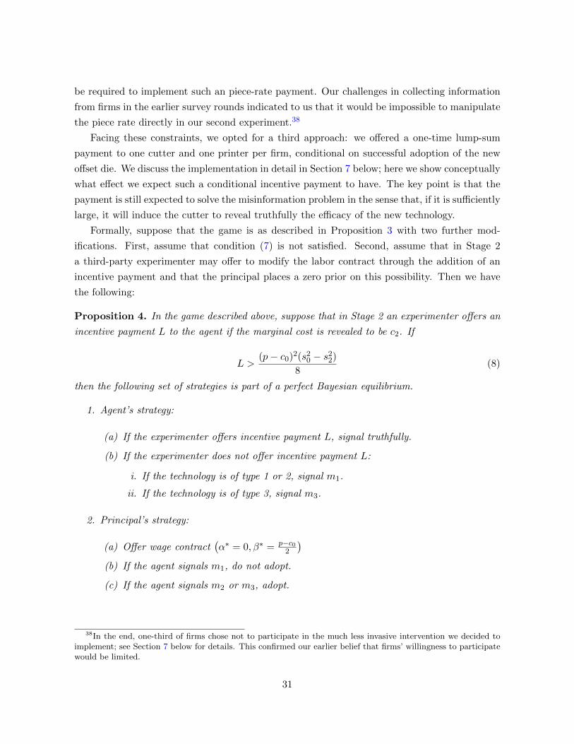
be required to implement such an piece-rate payment. Our challenges in collecting information

from firms in the earlier survey rounds indicated to us that it would be impossible to manipulate

the piece rate directly in our second experiment.38

Facing these constraints, we opted for a third approach: we offered a one-time lump-sum

payment to one cutter and one printer per firm, conditional on successful adoption of the new

offset die. We discuss the implementation in detail in Section 7 below; here we show conceptually

what effect we expect such a conditional incentive payment to have. The key point is that the

payment is still expected to solve the misinformation problem in the sense that, if it is sufficiently

large, it will induce the cutter to reveal truthfully the efficacy of the new technology.

Formally, suppose that the game is as described in Proposition 3 with two further mod-

ifications. First, assume that condition (7) is not satisfied. Second, assume that in Stage 2

a third-party experimenter may offer to modify the labor contract through the addition of an

incentive payment and that the principal places a zero prior on this possibility. Then we have

the following:

Proposition 4. In the game described above, suppose that in Stage 2 an experimenter offers an

incentive payment L to the agent if the marginal cost is revealed to be c2. If

L >(p− c0)2(s20 − s22)

8(8)

then the following set of strategies is part of a perfect Bayesian equilibrium.

1. Agent’s strategy:

(a) If the experimenter offers incentive payment L, signal truthfully.

(b) If the experimenter does not offer incentive payment L:

i. If the technology is of type 1 or 2, signal m1.

ii. If the technology is of type 3, signal m3.

2. Principal’s strategy:

(a) Offer wage contract(α∗ = 0, β∗ = p−c0

2

)(b) If the agent signals m1, do not adopt.

(c) If the agent signals m2 or m3, adopt.

38In the end, one-third of firms chose not to participate in the much less invasive intervention we decided toimplement; see Section 7 below for details. This confirmed our earlier belief that firms’ willingness to participatewould be limited.

31

The proof is in Appendix A.5. Intuitively, here the incentive payment, L, plays the same role

as the conditional piece rate γ∗∗ in Proposition 3: it raises the payoff to the agent of signaling

truthfully when the technology is of type 2. The empirical implication is simply that if the lump-

sum bonus is sufficiently large it will induce adoption of technology type 2. It is worth noting

that “sufficiently large” in this context is relative to the possible wage losses of a single cutter,

not to the revenues or profits of a firm. Indeed, we will see below that a lump-sum incentive

payment that appears small from the point of view of firms has a large effect on adoption,

consistent with this proposition.

7 Experiment 2: The Incentive-Payment Experiment

7.1 Experimental design

Motivated by the hypotheses described in the previous section, we conducted the incentive-

payment experiment in September-November 2013. To avoid interfering with the process of dif-

fusion to the non-tech-drop firms from the first experiment, we focused on only the 35 tech-drop

firms (including both initial responders and initial non-responders). At the time of random-

ization, we believed that 34 of these firms were still active. These were divided into the four

similarly-sized strata: (1) firms in the two smaller strata from the tech-drop experiment that

had not adopted the die as of August 2013, (2) firms in the two larger strata from the tech-drop

experiment that had not yet adopted the die, (3) firms from the initial non-responder stratum

from the tech-drop experiment that had not yet adopted the die, and (4) firms that had already

adopted the die. Within each stratum, firms were randomly assigned in equal proportion to

a treatment group (which we call Group A) and a control group (Group B). Three of the 34

assigned firms were subsequently revealed to have stopped manufacturing soccer balls, leaving

15 firms in Group A and 16 in Group B.

To firms in Group B we gave a reminder about the offset die and the new cutting pattern,

and informed them about the two-pentagon variant of the offset die (which, as noted above,

had proven more popular than the four-pentagon offset die we originally distributed.) We also

offered to do a new demonstration with their cutters. To each firm in Group A, we gave the

same refresher, the same offer of a new demonstration, and the same information about the

two-pentagon variant. In addition, we explained to the owner that cutters and printers paid

piece-rates had an incentive to misinform the owner about the value of the technology. We then

offered (to the owner) to pay one cutter and one printer lump-sum bonuses roughly equivalent

to their monthly incomes — 15,000 Rs (US$150) and 12,000 Rs (US$120), respectively — on

the condition that within one month the cutter demonstrate competence in using the new die

and the printer demonstrate competence in printing pairs of offset pentagon pieces cut by the

new die. If the owner agreed to the intervention, we explained the intervention to one cutter

32

and one printer chosen by the owner, paid them 1/3 of the incentive payment on the spot, and

scheduled a time to return to test their performance using the die.39

The performance target for cutters was 272 pentagons from a single sheet in three minutes

using the new die. The target for the printer was 48 pairs of pentagons cut by the offset

die in three minutes.40 We provided the owner with 20 laminated sheets for his workers to

practice with, printing screens for offset pentagon pairs, and a nominal Rs 5,000 ($50) to cover

additional costs such as overhead (e.g. electricity while the cutters were practicing). We returned

after approximately one month to test the employees and, upon successful achievement of the

performance targets, to pay the remaining 2/3 of the incentive payments. Without revealing

ahead of time that we would do so, we allowed for a buffer of 30 seconds and 5 pentagons for

cutters and 30 seconds for printers.41

Table 11 evaluates baseline balance by comparing firm characteristics across Group A and

Group B firms at the time of our visit to explain the intervention (September 2013). No differ-

ences in means are statistically significant. It appears that randomization was successful.42

7.2 Results

Ten of the 15 Group A firms agreed to participate in the experiment.43 Table 12 reports the

times achieved by the chosen cutter at each firm. The average time was 2 minutes and 52

seconds, approximately 27 percent longer than the average time to cut with the traditional die

(2 minutes and 15 seconds). The minimum time reported using the offset die was 2 minutes

and 28 seconds, or 9.6 percent longer than with the traditional die. It is partly for this reason,

and partly because cutters do not need to change sheets as frequently with the new die, that we

believe that the 50 percent increase in labor time factored into the cost calculations above in

Section 3 is conservative. In addition, many cutters expressed confidence that with additional

use they could lower their cutting time. All printers easily achieved their target, consistent with

the assumption in Section 3 that, despite some printers’ fears, the new die does not increase

labor time for printing.

39To the extent possible, we attempted to make the payment directly to the cutter and printer. In two cases,the owner insisted that we pay him and that he pass on the money to the employees, and we acceded to thisrequest.

40The 3-minute targets were chosen after conducting speed tests at two of the pilot firms mentioned in Section5. They are approximately one third higher than the time to cut a single sheet using the original die and the timeto print 48 two-pentagon panels cut using the original die.

41That is, the effective target for cutters was 267 pentagons from one sheet in 3 minutes 30 seconds, and forprinters was 48 pairs in 3 minutes 30 seconds.

42Because of an error by our enumerators, one firm that was assigned to Group B was offered the incentive-payment intervention. This occurred while two co-authors of the paper were in the field, and the error was caughtwithin hours of its occurrence. To maintain balance, we randomly selected one as-yet-untreated Group A firmfrom the same stratum and re-assigned it to Group B.

43In two of these 10 firms, it was not possible to complete the printer performance test.

33

In order to investigate adoption in response to the incentive-payment intervention, we carried

out a survey round in January-March 2014, 2-5 months after the completion of the intervention.44

As above, we classify a firm as an adopter if it reports that it is currently using the offset die and

has produced more than 1,000 balls with it in the past month. Of the 10 Group A firms that

agreed to participate in the experiment, two firms had already adopted the die at the time we

ran the incentive experiment. Of the remaining 8 firms, 5 firms subsequently adopted. Of the

16 Group B firms, 3 firms had already adopted prior to the invention. None of the remaining

13 firms subsequently adopted.

Table 13 formally assesses the impact of the incentive-payment intervention on adoption

rates. All regressions include dummies for the four strata described above. Columns 1-4 include

all strata, and Columns 5-8 omit the stratum of firms that had already adopted by August

2013. The first-stage estimates (Columns 1 and 5) indicate, not surprisingly, that assignment to

Group A is significantly associated with greater probability of receiving the incentive-payment

treatment; that is, we have a strong first stage. The dependent variable in Columns 2-4 and 6-8

is a 0/1 indicator for whether a firm has adopted, i.e. is currently using the offset die and has

produced more than 1,000 balls using it. The OLS estimates in Columns 2 and 6 are positive

and significant, but one might be worried about selection into treatment. The reduced-form

(intent-to-treat) results in Columns 3 and 7 do not suffer from such selection issues and indicate

a positive and significant (at the 5 percent level) causal relationship between assignment to

Group A and adoption. Adoption rates increased by 0.32 among the treatment group or by

0.38 if we restrict attention to only the firms who had not already adopted at the start of the

experiment. The IV estimates (the effect of treatment on the treated) are substantially higher

(0.48 or 0.63 if we restrict attention only to initial non-adopters). However, since the one third

of firms who refused the intervention may have chosen to do so because of particularly large

costs of adoption (or small benefits), these IV estimates should be treated with caution.

To check robustness, Table 14 reports results using an alternative indicator of adoption,

namely whether the firm purchased its first offset die (beyond the trade-in that we paid for)

after September 1, 2013. Of the eight firms that accepted the intervention and had not adopted

by August 2013, three subsequently purchased their first offset die. (One of these firms had not

produced with it yet at the time of our most recent survey.)45 Table 14 shows that the positive

causal effect of the incentive-payment treatment on adoption is robust to using this alternative

measure.

It is important to acknowledge that the sample sizes in the incentive-payment experiment are

44In one case, the firm’s report regarding adoption was ambiguous and our enumerators followed up with thefirm to clarify in May 2014.

45In addition, one large Group-A firm that was already classified as an adopter because it was using the offsetcutting pattern for table cutting (see footnote 12), purchased its first die (beyond the four-panel offset die weoriginally gave) following the beginning of our intervention.

34

small. An alternative to large-N statistical inference are permutation tests whose properties are

independent of sample size (see Bloom, Eifert, Mahajan, McKenzie, and Roberts (2013) for the

use of this type of inference in a similar context). We determine the proportion of all possible

treatment assignments that produce coefficients as large as or larger than the ones we find. This

procedure produces an exact p-value and does not require any asymptotic approximations. Given

the selection discussion above, we focus on the more conservative ITT estimates in columns 3

and 7 of Tables 13 and 14. Within each of the four strata, we assigned treatment status with 50

percent probability. The stratum of smaller firms contained 6 firms, the stratum of larger firms

contained 12 firms, the stratum of initial non-responders contained 8 firms and the stratum of

already-adopters contained 5 firms. This means there are 25, 872, 000 =(63

)(126

)(84

)((52

)+(53

))possible treatment assignments.46

Figure 16 plots the distribution of coefficients obtained from regressing die use on assignment

to group A for the millions of possible treatment assignments. The left panel reports the distri-

bution of outcomes under the specifications with all strata and the right panel reports outcomes

from the initial non-adopters sample only. The vertical line in both figures denotes the observed

ITT effects reported in columns 3 and 7 of Table 13. Note that there are only a handful of

possible coefficients despite the several million possible permutations. This is because of the

small number of adopting firms and because no control firm has adopted the die. Yet in both

cases, the observed ITT coefficients are the largest effects that could have been observed under

any treatment assignment. In other words, there is no possible outcome that is more extreme

than the one we observe in each specification. We can use the distribution to construct p-values

for the hypothesis test that the coefficients we find are different from zero. For our main measure

of adoption, current use, the p-value is 3.04 percent in both the all firm and initial non-adopter

samples. Figure 17 presents a similar analysis for our alternative indicator of adoption, die

purchases, with corresponding p-values of 4.28 percent in the all-firm sample and 21.42 percent

in the initial non-adopters sample.

The results indicate a robust effect of the incentive payment treatment on adoption. Con-

sidering current use (> 1, 000 balls) as the outcome, it is striking that over half of the treated

firms that had not previously adopted responded to the treatment. As we discuss in the next

section, It seems hard to rationalize such a large response to such a small incentive, unless the

incentive is helping to resolve an organizational bottleneck within the firm.

7.3 Examining Alternative Explanations for Increase in Take-up

In this sub-section, we examine two alternative explanations for our finding that a small incentive

payment substantially increased adoption.

46If we exclude the already-adopter stratum, there are 1, 293, 600 =(63

)(126

)(84

)possible permutations.

35

7.3.1 Alternative hypothesis: subsidies for fixed costs

The first alternative we consider is that there was no information transmission from workers

to owners, but that we mechanically induced firms to adopt by subsidizing the fixed costs of

adoption. This explanation is best seen through the lens of the model. In the model, suppose

that the owner is aware of conditional wage contracts and that there is no cost of using them,

G = 0. The owner then simply weighs the variable cost reduction from the new technology

against the fixed costs of adoption. These fixed costs may include a lump-sum wage bonus to

workers to compensate them for a learning period where they will earn less. Our incentive-

payment experiment could be seen as providing a subsidy to cover some of these fixed costs of

adoption, and the subsidy may itself have induced the owner to adopt.

Is this a quantitatively plausible explanation of our findings? To organize our thinking

about this question, we can write the present discounted value of expected additional profit

from adoption for firm f as follows:

Πf = −FCf0 + Pr(success)f

∞∑t=1

NV Bf(1 + rf )t

(9)

where FCf0 are fixed costs of adoption, which must be paid up front and may be firm-specific;

Pr(success)f is the probability perceived by the firm that the technology works as we said it

does; NV Bf are net variable benefits per cutter per month; and rf is the interest rate faced

by the firm. Net Variable Benefits can be calculated for each firm following the method of

Section 3.2. For firms that did not have to buy the die, which correspond to the tech-drop

firms in the incentive-payment experiment, observed fixed costs are Rs 10,800/US$108.47 In

this section, we make the assumption that the Rs 32,000/US$32048 we paid in the incentive-

payment treatment were also necessary and part of the true fixed cost of adoption.49 We thus

take the total observed fixed costs to be Rs 42,800/US$428.50 The assumption regarding wage

payments seems conservative. In the incentive-payment experiment, only one worker felt that the

payment was insufficient to cover his costs of adoption, suggesting that the incentive payments

were greater than the “training” cost faced by workers in the great majority of firms.

As a first step toward answering the quantitative plausibility question, suppose that there

47Rs 800/US$8 to have screens redesigned and remade and Rs 10,000/US$100 for a new die for the hole-punching machine; see Section 3.2 for further details.

48Rs 15,000/US$150 to the cutter, Rs 12,000/US$120 to the printer, plus Rs 5,000/US$50 to the owner tocover overhead.

49In Section 3.2 we assumed that workers wages went up by 50% to compensate them for using the slowertechnology. The discussion in Section 6 suggests that many firms do not adjust their wages and so in this sectionwe remove this component and instead assume that the firm must only pay the one-off conditional wage payment.

50This calculation uses net variable benefits per cutter since we assume that the fixed costs need to be paidfor each cutter in the firm. This is a conservative assumption since it is possible that firms could, for example,share the hole-punching machine across cutters.

36

is no uncertainty about the technology (i.e. Pr(success)f = 1) and no unobserved fixed costs

beyond the US$428 mentioned above. Under these assumptions, (9) can be reconciled with

non-adoption only if firms face extremely high interest rates and hence have a small effective

discount factor 1/(1 + rf ).51 For initial non-adopters, the values of firm-specific interest rates

that set Πf = 0 in (9) represent lower bounds on the firm-specific interest rates. At the 10th

percentile, the lower bound is 7.8% per month; at the 90th percentile, the lower bound is 70.7%

per month. In our baseline survey, we asked firms explicitly about the interest rates they face,

and the responses ranged from 3% to 19% per year ; these are an order of magnitude lower than

the implied lower bound for most firms. That is, in the absence of both uncertainty about the

technology and unobserved fixed costs, the interest rates (and rate of discounting) that would

be required to explain the low initial rates of adoption appear to be implausibly high.

This argument leaves open the possibility that some combination of uncertainty and unob-

served fixed costs can account for the low initial rates of adoption we observed. To address this

possibility, we take a different approach: we allow for uncertainty and unobserved fixed costs

and ask whether these can explain both the low rates of initial adoption and the magnitude of

the response to our incentive-payment intervention. The unobserved fixed costs may represent

attention costs for the owner or psychic costs involved in changing established routines. We as-

sume, conservatively, that the interest rate is the highest of the self-reported interest rates, 19%

per year. As a benchmark, we assume that owners place a 50% probability on the event that

the technology works as we described (i.e. Pr(success)f = .5); we consider alternative priors

below. Under these assumptions, we can place bounds on the values of unobserved fixed costs

that can explain the behavior we observe.52 These bounds on fixed costs are plotted by rank in

Figure 18 for the 31 firms in the incentive-payment experiment. The black outlines represent

the lower bounds that would be implied by non-adoption, and the red outlines the upper bounds

that would be implied by adoption in response to the incentive-payment intervention.53

There are two important points to notice in Figure 18. The first is that, for almost all

firms, the US$320 subsidy is small relative to the implied lower bound on fixed costs. At the

10th percentile, the implied lower bound on fixed costs is US$2,286; at the 90th percentile, it

is US$20,718. For the vast majority of firms the implied fixed costs are an order of magnitude

greater than the subsidy. The second point to note is that the firms’ lower bounds are not

bunched closely together. Therefore, if a substantial portion of the unobserved fixed costs is

51This is another way of stating the argument from Section 3.2.3 that the observable fixed costs of adoptioncan be recouped within a relatively short amount of time by almost all firms.

52In particular, simplifying (9), if a firm does not adopt initially, it must be that Πf < 0 and hence that

FCf0 > (.5)NV Bf

.0146. If a firm adopts in response to the incentive-payment experiment, it must be that Πf > 0

after the US$320 reduction in fixed costs, and hence that FCf0 < (.5)NV Bf

.0146+ 320.

53Firms that initially adopted are indicated by the sold black bars; for these firms, we can conclude only thatfixed costs are less than what is indicated by the black outline. The firms that adopted in experiment 2 areindicated by solid green bars.

37

common across firms, a subsidy of US$320 would only lead to a few firms adopting and hence

ITT coefficients much smaller than the ones we found.

We can make these claims more precise by imposing some structure on the distribution of

unobserved fixed costs. Suppose that fixed costs are distributed log normally:

ln(FC0f ) = θ + εf (10)

where εf ∼ N (0, σ2ε). We can use information on adoption in both experiments 1 and 2 to

estimate θ and the error variance, σ2ε .54 Panel A of Table 15 reports these estimates θ and σ2ε

under six priors ranging from Pr(success)f = .01 to Pr(success)f = 1.

With these estimates in hand, we can ask: what is the probability that we would observe

an effect of a US$320 subsidy on adoption as large as the effect we observed in experiment 2?

To answer this question we use θ and σ2ε to simulate 1,000 fixed cost draws, with Figure 19

displaying the full distribution of Group A firms switching from non-adoption to adoption as a

result of a US$320 payment. Panel B of Table 15 reports the corresponding probabilities of 5

or more Group A firms switching. The probability of observing an increase in adoption of that

magnitude is exceedingly low, between .000 and .003, for all but the most pessimistic prior of

Pr(success)f = .01. Although such a low prior is theoretically possible, it seems unrealistically

pessimistic given the nature of the technology.

In Panel C of Table 15, we turn to the corresponding ITT estimates from these simula-

tions. The ITT estimates range between .01 and .08 for priors between Pr(success)f = 1 and

Pr(success)f = .05, much lower than the 0.32 we obtained in our incentive-payment experi-

ment. Even for the most pessimistic prior of Pr(success)f = .01, we only obtain an ITT of

0.22. In summary, a US$320 subsidy cannot plausibly explain the magnitude of the increase in

adoption we observed in our second experiment. Even when we choose the mean and variance

54We estimate the parameters using maximum likelihood. Let adopt1f denote an indicator if firm f had adoptedthe technology in experiment 1, and adopt2,f an analogous indicator for adoption after experiment 2. The loglikelihood function for group A firms is:

l(θ, σε) =∑f

(1− adopt1f )(adopt2f ) ln

[Φ

(ln(NV Bf + 320)− θ

σε

)− Φ

(ln(NV Bf )− θ

σε

)](11)

+(1− adopt1f )(1− adopt2f ) ln

[1− Φ

(ln(NV Bf + 320)− θ

σε

)]+(adopt1f ) ln

[Φ

(ln(NV Bf )− θ

σε

)]The first expression on the right-hand-side of (11) captures the contribution to the likelihood of initial non-adoptergroup-A firms who are induced to switch from non-adoption to adoption because of the $320 subsidy. The secondexpression captures initial non-adopter group-A firms who are not induced to switch adoption status. The thirdexpression is the contribution of initial adopter firms. We jointly maximize the likelihood function with the groupB firms who have the same likelihood function except adopt2f = 0 ∀f and there is no US$320 payment inside theargument of the normal CDF, Φ(.).

38

of the unobserved fixed costs to best fit the adoption patterns in experiments 1 and 2, a US$320

subsidy can only generate our experimental findings under extremely pessimistic priors.

7.3.2 Alternative hypothesis: salience

A second alternative explanation is that the incentive-payment treatment increased the salience

of the new technology and this itself led firms to adopt, independent of any effects on information

flows within the firm. There are two variants of this explanation. One variant is that the

reminder about the technology during the incentive-intervention visit itself “nudged” firms into

adoption. This variant can be quickly dismissed. We gave the same reminder to the control

firms for the incentive intervention (Group B firms) and we saw no firms adopt subsequently as

a result. Also, it is worth noting that we visited all of the tech-drop firms multiple times as part

of our survey rounds. During each of these visits, we discussed the new technology with them

and if they were not using it we asked why.

A different variant of the salience story is that by putting more money on the table we sent

a stronger signal about our own beliefs about the efficacy of our technology, and this in turn

led firms to update their priors about the technology, inducing some firms to adopt. While it

is difficult to dismiss this explanation definitively, it also seems unlikely. We believe that it was

clear to firms from the outset, in the initial technology-drop implementation, that we believed

that the technology was effective. We said so in the initial treatment, and we then demonstrated

the efficacy of the technology using firms’ own cutters. We then returned to each firm numerous

times and, as noted above, in the case of the tech-drop firms we discussed the offset die each

time. The amount of money we spent on surveying each firm far exceeded the US$320 payment

in the incentive intervention. In short, while in retrospect it seems clear that many owners

did not believe us when we told them that the technology works, it does not appear that their

skepticism was based on their beliefs about how strongly we held our beliefs, or that the US$320

affected their beliefs about how strongly we held our beliefs. It seems more likely that they

believed that we simply had insufficient knowledge and experience in the industry, and hence

that our (strongly held) confidence in the technology was misplaced.

8 Conclusion

This paper has two basic empirical findings. First, despite the evident advantages of the tech-

nology we invented, a surprisingly small number of firms have adopted it, even among the set

of firms that we gave it to. This is consistent with a long tradition of research on technology

adoption that has found diffusion to be slow for some technologies, but given the characteristics

of our technology — low fixed costs, minimal required changes to other aspects of the produc-

tion process, limited uncertainty about the cost advantage of the technology — the low adoption

39

rate seems particularly puzzling. Second, with a very small change in the incentives facing key

employees in the firm — tiny in monetary terms relative to firms’ revenues and the benefits of

adoption — we induced a statistically significant increase in adoption. This is consistent with

the hypothesis that a misalignment of incentives within the firm — in particular, employees

paid piece rate have an incentive to resist adoption of a material-saving technology that slows

them down — is an important barrier to adoption. Although for most firms we do not observe

directly the communication between employees and owners, it appears that at least one way that

employees have resisted the adoption of our new technology is by misinforming owners about

the value of the technology. It further appears that the incentive-payment intervention had a

significant effect because it induced workers to report truthfully to owners.

The natural question is why many owners did not simply change the payment scheme on

their own. We have considered two possible explanations. One is that they were not aware

of the availability of alternative payment schemes, or did not understand that an alternative

scheme would be desirable. A second possibility is that there are transaction costs involved in

changing contracts, even implicit ones. Above we discussed a number of possible reasons for the

existence of such costs. Whatever their source, owners may weigh any costs of modifying con-

tracts against the expected benefits of adopting new technologies. If owners have low priors that

a beneficial new technology will arrive (or that a technology that has arrived is beneficial), they

may rationally be unwilling to pay even quite small transaction costs. These two explanations

for the stickiness of wage contracts have similar observable implications, and it is difficult for us

to distinguish between them in our context. At the same time, the key point for our study is

that many firms did not in fact change their payment schemes, and this left scope for our very

modest intervention to have a large effect on adoption.

Although our empirical results are clearly specific to the setting we study, our findings suggest

three implications that we believe are likely to apply more broadly. First, we have provided

reasonably direct evidence evidence of a complementarity, in the sense of Milgrom and Roberts

(1990, 1995), between a technological innovation (the new die) and an organizational innovation

(conditional wage contracts). We suspect that similar complementarities between technical and

organizational innovations exist in many other settings. This in turn suggests that the study of

adoption of particular technologies cannot be divorced from the study of organizational change

in the firms doing the adopting.

Second, there appears to be a form of inertia in employment relationships that can hinder

technological change. We have argued that firms’ choices of labor contracts depend on the rate

at which beneficial new technologies are expected to arrive. It also appears that labor contracts,

once established, may be difficult to modify. The implication is that industries that evolve in

technologically stable environments may be less able to adapt to technological change than new

industries. Simple piece-rate contracts may well have been optimal in Sialkot before we showed

40

up, but the very fact that firms in Sialkot have been producing for decades using piece-rates and

the same basic production process may itself have contributed to low adoption rates of the new

die.

Finally, it seems likely that in order for technology adoption to be successful employees have

to have an expectation that they will share in the gains from adoption. Such an expectation

may be generated by a variety of different types of contracts, implicit or explicit. But to the

extent that owners and managers must rely on the knowledge of shopfloor workers about the

value of new technologies or how best to implement them, it appears to be important that a

credible gain-sharing mechanism be in place.

41

References

Anderson, S. T., and R. G. Newell (2004): “Information Programs for Technology Adoption: TheCase of Energy-Efficiency Audits,” Resource and Energy Economics, 26(1), 27 – 50.

Atkin, D., A. Chaudhry, S. Chaudry, A. K. Khandelwal, and E. Verhoogen (2014): “Technol-ogy Spillovers among Manufacturing Firms: Evidence from Pakistan,” Mimeo, Columbia University.

Bandiera, O., I. Barankay, and I. Rasul (2005): “Social Preferences and the Response to Incentives:Evidence from Personnel Data,” Quarterly Journal of Economics, 120(3), pp. 917–962.

(2007): “Incentives for Managers and Inequality among Workers: Evidence from a Firm-LevelExperiment,” Quarterly Journal of Economics, 122(2), pp. 729–773.

(2009): “Social Connections and Incentives in the Workplace: Evidence from Personnel Data,”Econometrica, 77(4), pp. 1047–1094.

(2011): “Field Experiments with Firms,” The Journal of Economic Perspectives, 25(3), pp.63–82.

Bandiera, O., and I. Rasul (2006): “Social Networks and Technology Adoption in Northern Mozam-bique,” Economic Journal, 116(514), 869 – 902.

Beaman, L., J. Magruder, and J. Robinson (2014): “Minding Small Change among Small Firmsin Kenya,” Journal of Development Economics, 108(0), 69 – 86.

BenYishay, A., and A. M. Mobarak (2014): “Social Learning and Communication,” NBER workingpaper no. 20139.

Bloom, N., B. Eifert, A. Mahajan, D. McKenzie, and J. Roberts (2013): “Does ManagementMatter? Evidence from India,” Quarterly Journal of Economics, 128(1), 1–51.

Bloom, N., and J. Van Reenen (2007): “Measuring and Explaining Management Practices AcrossFirms and Countries,” The Quarterly Journal of Economics, 122(4), 1351–1408.

(2010): “Why Do Management Practices Differ across Firms and Countries?,” Journal of Eco-nomic Perspectives, 24(1), 203–24.

Bresnahan, T. F., and M. Trajtenberg (1995): “General Purpose Technologies: ‘Engines ofGrowth’?,” Journal of Econometrics, 65(1), 83 – 108.

Carmichael, H. L., and W. B. MacLeod (2000): “Worker Cooperation and the Ratchet Effect,”Journal of Labor Economics, 18(1), 1–19.

Clawson, D. (1980): Bureaucracy and the Labor Process: The Transformation of US Industry, 1860-1920. Monthly Review Press New York.

Cohen, J., and P. Dupas (2010): “Free Distribution or Cost-Sharing? Evidence from a RandomizedMalaria Prevention Experiment,” Quarterly Journal of Economics, 125(1), 1–45.

Coleman, James, E. K., and H. Menzel (1966): Medical Innovation: A Diffusion Study. Bobbs-Merrill, New York.

Conley, T., and C. Udry (2010): “Learning about a New Technology: Pineapple in Ghana,” AmericanEconomic Review, 100(1), 35–69.

Crawford, V. P., and J. Sobel (1982): “Strategic Information Transmission,” Econometrica, pp.1431–1451.

David, P. A. (1990): “The Dynamo and the Computer: An Historical Perspective on the ModernProductivity Paradox,” American Economic Review Papers and Proceedings, 80(2), 355–61.

de Mel, S., D. J. McKenzie, and C. Woodruff (2008): “Returns to Capital in Microenterprises:Evidence from a Field Experiment,” Quarterly Journal of Economics, 123(4), 1329–1372.

Dearden, J., B. W. Ickes, and L. Samuelson (1990): “To Innovate or Not to Innovate: Incentivesand Innovation in Hierarchies,” The American Economic Review, 80(5), pp. 1105–1124.

Desmet, K., and S. L. Parente (forthcoming): “Resistance to Technology Adoption: The Rise andDecline of Guilds,” Forthcoming, Review of Economic Dynamics.

Dessein, W. (2002): “Authority and Communication in Organizations,” Review of Economic Studies,

42

69(4), 811 – 838.

Duflo, E., M. Kremer, and J. Robinson (2011): “Nudging Farmers to Use Fertilizer: Theory andExperimental Evidence from Kenya,” American Economic Review, 101(6), 2350–2390.

Dupas, P. (2014): “Short-run Subsidies and Long-Run Adoption of New Health Products: Evidencefrom a Field Experiment,” Econometrica, 82(1), 197–228.

Edwards, R. C. (1979): Contested Terrain: The Transformation of the Workplace in the TwentiethCentury. Basic Books.

Foster, A. D., and M. R. Rosenzweig (1995): “Learning by Doing and Learning from Others:Human Capital and Technical Change in Agriculture,” Journal of Political Economy, 103, 1176–1209.

Freeman, R. B., and M. M. Kleiner (2005): “The Last American Shoe Manufacturers: DecreasingProductivity and Increasing Profits in the Shift from Piece Rates to Continuous Flow Production,”Industrial Relations: A Journal of Economy and Society, 44(2), 307–330.

Geroski, P. A. (2000): “Models of Technology Diffusion,” Research Policy, 29(45), 603 – 625.

Gibbons, R. (1987): “Piece-Rate Incentive Schemes,” Journal of Labor Economics, pp. 413–429.

Gibbons, R., and J. Roberts (2013): “Economic Theories of Incentives in Organizations,” in Handbookof Organizational Economics, ed. by R. Gibbons, and J. Roberts. Princeton: Princeton UniversityPress.

Griliches, Z. (1957): “Hybrid Corn: An Exploration in the Economics of Technological Change,”Econometrica, 25(4), 501–22.

Hall, B. (2005): “Innovation and Diffusion,” in Oxford Handbook of Innovation, ed. by J. Fagerberg,D. C. Mowery, and R. R. Nelson, pp. 459–484. Oxford University Press.

Hall, B., and B. Khan (2003): “Adoption of New Technology,” in New Economy Handbook, ed. byD. C. Jones. Academic Press, San Diego.

Hanna, R., S. Mullainathan, and J. Schwartzstein (forthcoming): “Learning Through Noticing:Theory and Experimental Evidence in Farming,” Forthcoming, Quarterly Journal of Economics.

Holmstrom, B., and P. Milgrom (1991): “Multi-Task Principal-Agent Analyses: Incentive Contracts,Asset Ownership and Job Design,” Journal of Law, Economics and Organization, 7, 24–52.

Houreld, K. (2014): “Pakistan Ball Maker to Fulfill World Cup Dream,” Reuters,May 21, 2014. http://www.reuters.com/article/2014/05/21/us-soccer-world-pakistan-ball-idUSKBN0E01FE20140521.

Ichniowski, C., and K. Shaw (2013): “Insider Econometrics,” in Handbook of Organizational Eco-nomics, ed. by R. Gibbons, and J. Roberts. Princeton: Princeton University Press.

Khan, F. R., K. A. Munir, and H. Willmott (2007): “A Dark Side of Institutional Entrepreneurship:Soccer Balls, Child Labour and Postcolonial Impoverishment,” Organization Studies, 28(7), 1055–1077.

Khwaja, A., B. Olken, and A. Q. Khan (2014): “Tax Farming Redux: Experimental Evidence onIncentive Pay for Tax Collectors,” Unpub. paper, Harvard.

Krishna, V., and J. Morgan (2008): “Contracting for Information under Imperfect Commitment,”RAND Journal of Economics, 39(4), 905 – 925.

Kuperberg, G., and W. Kuperberg (1990): “Double-Lattice Packings of Convex Bodies in thePlane,” Discrete & Computational Geometry, 5, 389–397.

Lazear, E. P. (1986): “Salaries and Piece Rates,” The Journal of Business, 59(3), pp. 405–431.

Lazear, E. P., and P. Oyer (2013): “Personnel Economics,” in Handbook of Organizational Eco-nomics, ed. by R. Gibbons, and J. Roberts. Princeton: Princeton University Press.

Lazonick, W. (1979): “Industrial Relations and Technical Change: The Case of the Self-Acting Mule,”Cambridge Journal of Economics, 3(3), pp. 231–262.

Lefley, F. (1996): “The Payback Method of Investment Appraisal: A Review and Synthesis,” Interna-tional Journal of Production Economics, 44(3), 207 – 224.

Mansfield, E. (1961): “Technical Change and the Rate of Imitation,” Econometrica, 29(4), pp. 741–766.

(1989): “The Diffusion of Industrial Robots in Japan and the United States,” Research Policy,

43

18(4), 183 – 192.

Miguel, E., and M. Kremer (2004): “Worms,” Econometrica, 72(1), 159–217.

Milgrom, P., and J. Roberts (1990): “The Economics of Modern Manufacturing: Technology, Strat-egy and Organization,” American Economic Review, 80(3), 511–528.

(1995): “Complementarities and Fit: Strategy, Structure and Organizational Change in Manu-facturing,” Journal of Accounting and Economics, 19, 179–208.

Mokyr, J. (1990): The Lever of Richies. Oxford University Press.

Munshi, K. (2004): “Social Learning in a Heterogeneous Population: Technology Adoption in the IndianGreen Revolution,” Journal of Development Economics, 73, 185–213.

Parente, S., and E. Prescott (1999): “Monopoly Rights: A Barrier to Riches,” American EconomicReview, 89(5), 1216–1233.

Rosenberg, N. (1982): Inside the Black Box: Technology and Economics. Cambridge UK: CambridgeUniversity Press.

Ryan, B., and N. C. Gross (1943): “Diffusion of Hybrid Seed Corn in Two Iowa Communities,” RuralSociology, 8, 15–24.

Sandal, M. I. (undated): History of Football and Pakistan’s Contribution. Self-published.

Sobel, J. (2013): “Giving and Receiving Advice,” in Advances in Economics and Econometrics, ed. byD. Acemoglu, M. Arellano, and E. Dekel. Cambridge University Press.

Stoneman, P. (2002): The Economics of Technological Diffusion. Blackwell, Oxford.

Suri, T. (2011): “Selection and Comparative Advantage in Technology Adoption,” Econometrica, 79(1),159–209.

Syverson, C. (2011): “What Determines Productivity?,” Journal of Economic Literature, 49(2), 326–65.

Tybout, J. (2000): “Manufacturing Firms in Developing Countries: How Well Do They Do, and Why?,”Journal of Economic Literature, 38, 11–44.

Wright, T. (2010): “Pakistan Defends Its Soccer Industry,” Wall Street Journal, April 26, 2010.

44

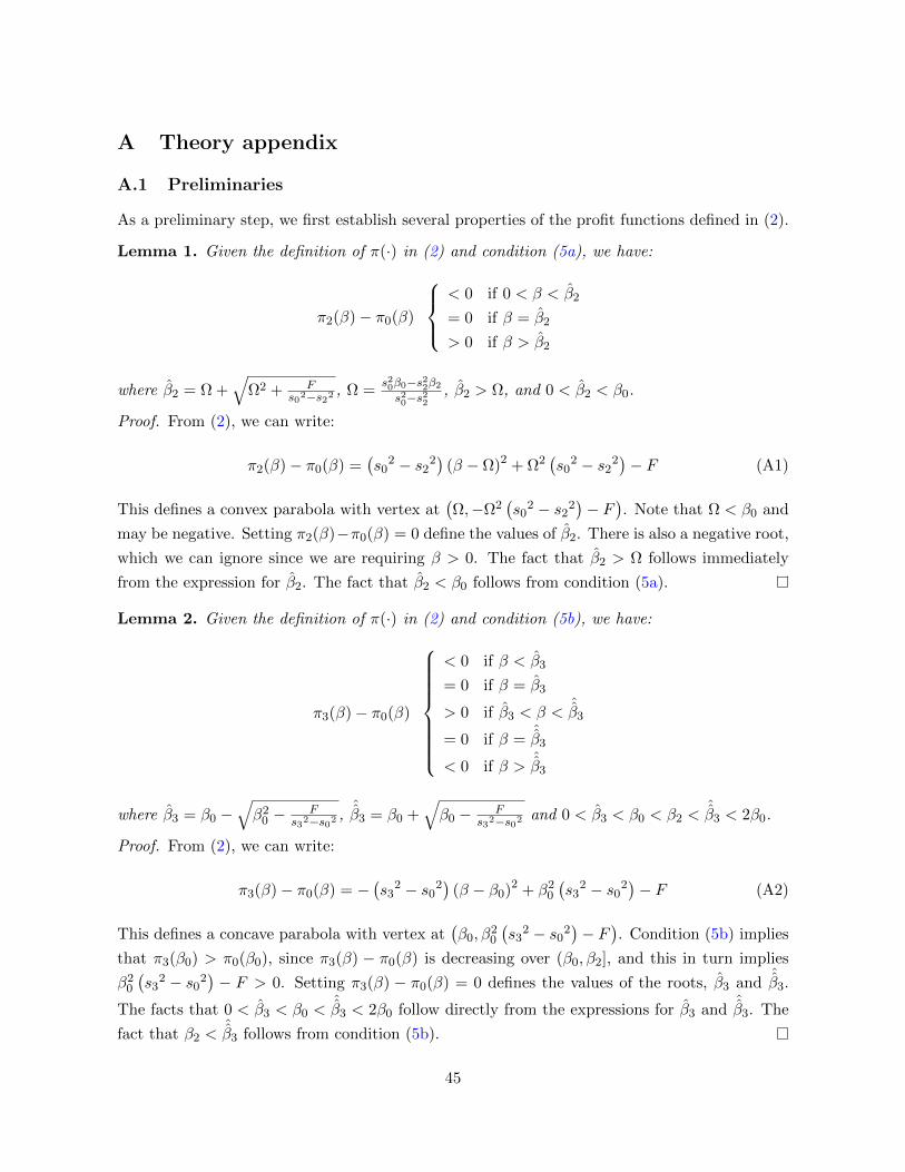
A Theory appendix

A.1 Preliminaries

As a preliminary step, we first establish several properties of the profit functions defined in (2).

Lemma 1. Given the definition of π(·) in (2) and condition (5a), we have:

π2(β)− π0(β)

< 0 if 0 < β < β2

= 0 if β = β2

> 0 if β > β2

where β2 = Ω +√

Ω2 + Fs02−s22 , Ω =

s20β0−s22β2s20−s22

, β2 > Ω, and 0 < β2 < β0.

Proof. From (2), we can write:

π2(β)− π0(β) =(s0

2 − s22)

(β − Ω)2 + Ω2(s0

2 − s22)− F (A1)

This defines a convex parabola with vertex at(Ω,−Ω2

(s0

2 − s22)− F

). Note that Ω < β0 and

may be negative. Setting π2(β)−π0(β) = 0 define the values of β2. There is also a negative root,

which we can ignore since we are requiring β > 0. The fact that β2 > Ω follows immediately

from the expression for β2. The fact that β2 < β0 follows from condition (5a).

Lemma 2. Given the definition of π(·) in (2) and condition (5b), we have:

π3(β)− π0(β)

< 0 if β < β3

= 0 if β = β3

> 0 if β3 < β <ˆβ3

= 0 if β =ˆβ3

< 0 if β >ˆβ3

where β3 = β0 −√β20 − F

s32−s02 ,ˆβ3 = β0 +

√β0 − F

s32−s02 and 0 < β3 < β0 < β2 <ˆβ3 < 2β0.

Proof. From (2), we can write:

π3(β)− π0(β) = −(s3

2 − s02)

(β − β0)2 + β20(s3

2 − s02)− F (A2)

This defines a concave parabola with vertex at(β0, β

20

(s3

2 − s02)− F

). Condition (5b) implies

that π3(β0) > π0(β0), since π3(β) − π0(β) is decreasing over (β0, β2], and this in turn implies

β20(s3

2 − s02)− F > 0. Setting π3(β) − π0(β) = 0 defines the values of the roots, β3 and

ˆβ3.

The facts that 0 < β3 < β0 <ˆβ3 < 2β0 follow directly from the expressions for β3 and

ˆβ3. The

fact that β2 <ˆβ3 follows from condition (5b).

45

Lemma 3. Given the definition of π(·) in (2), we have:

π1(β)− π0(β)

< 0 if 0 < β <

ˆβ1

= 0 if β =ˆβ1

> 0 if β >ˆβ1

whereˆβ1 = β0 +

√β20 + F

s02−s12 > 2β0.

Proof. From (2), we can write

π1(β)− π0(β) =(s0

2 − s12)

(β − β0)2 −(s0

2 − s12)β20 − F (A3)

which is a convex parabola with roots β1 = β0−√β20 + F

s02−s12 < 0 andˆβ1 defined above. Since

we have assumed β > 0, β1 will not play a role.

A.2 Proof of Proposition 1

Let µ(tj |mi, β) be the principal’s belief that the technology is type j, given the agent’s signal

mi and the piece rate β. Recall that the principal’s priors are ρ1, ρ2 and ρ3. Since m2 is

never signaled on the equilibrium path, µ(t2|m2, β∗) is an off-path belief and we specify it

to be 1. The principal’s beliefs after Stage 3 are then: µ(t1|m1, β∗) = ρ1

ρ1+ρ2, µ(t2|m1, β

∗) =ρ2

ρ1+ρ2, µ(t2|m2, β

∗) = 1, µ(t3|m3, β∗) = 1.

To prove the proposition, it suffices to show that there is no profitable deviation for either

principal or agent.

A.2.1 No Incentive For Agent to Deviate

First we show there is no incentive for the agent to deviate from his signaling strategy holding

fixed the principal’s strategy. Note that conditional on the piece rate being held fixed, the agent

strictly prefers faster technologies since his utility is increasing in s:

U(β, s) =β2s2

2(A4)

For a given piece rate, β, there are three states of the world to consider:

1. If the technology is of type 1, the agent signals m1 and the principal does not adopt. The

agent has no incentive to deviate and signal m2 or m3, which will induce the principal to

adopt, since s1 < s0.

2. If the technology is of type 2, the agent signals m1. The agent does not have an incentive

to deviate and signal m2 or m3 as this would induce adoption and s2 < s0.

46

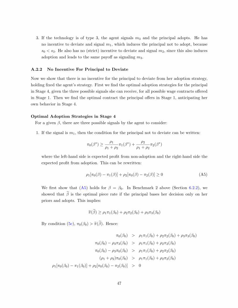
3. If the technology is of type 3, the agent signals m3 and the principal adopts. He has

no incentive to deviate and signal m1, which induces the principal not to adopt, because

s0 < s3. He also has no (strict) incentive to deviate and signal m2, since this also induces

adoption and leads to the same payoff as signaling m3.

A.2.2 No Incentive For Principal to Deviate

Now we show that there is no incentive for the principal to deviate from her adoption strategy,

holding fixed the agent’s strategy. First we find the optimal adoption strategies for the principal

in Stage 4, given the three possible signals she can receive, for all possible wage contracts offered

in Stage 1. Then we find the optimal contract the principal offers in Stage 1, anticipating her

own behavior in Stage 4.

Optimal Adoption Strategies in Stage 4

For a given β, there are three possible signals by the agent to consider:

1. If the signal is m1, then the condition for the principal not to deviate can be written:

π0(β∗) ≥ ρ1

ρ1 + ρ2π1(β

∗) +ρ2

ρ1 + ρ2π2(β

∗)

where the left-hand side is expected profit from non-adoption and the right-hand side the

expected profit from adoption. This can be rewritten:

ρ1[π0(β)− π1(β)] + ρ2[π0(β)− π2(β)] ≥ 0 (A5)

We first show that (A5) holds for β = β0. In Benchmark 2 above (Section 6.2.2), we

showed that β is the optimal piece rate if the principal bases her decision only on her

priors and adopts. This implies:

π(β) ≥ ρ1π1(β0) + ρ2π2(β0) + ρ3π3(β0)

By condition (5c), π0(β0) > π(β). Hence:

π0(β0) > ρ1π1(β0) + ρ2π2(β0) + ρ3π3(β0)

π0(β0)− ρ3π3(β0) > ρ1π1(β0) + ρ2π2(β0)

π0(β0)− ρ3π0(β0) > ρ1π1(β0) + ρ2π2(β0)

(ρ1 + ρ2)π0(β0) > ρ1π1(β0) + ρ2π2(β0)

ρ1[π0(β0)− π1(β0)] + ρ2[π0(β0)− π2(β0)] > 0

47

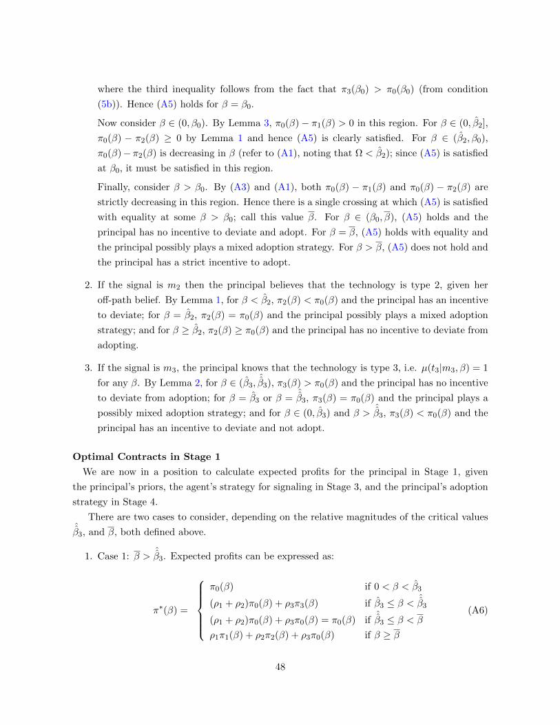
where the third inequality follows from the fact that π3(β0) > π0(β0) (from condition

(5b)). Hence (A5) holds for β = β0.

Now consider β ∈ (0, β0). By Lemma 3, π0(β)− π1(β) > 0 in this region. For β ∈ (0, β2],

π0(β) − π2(β) ≥ 0 by Lemma 1 and hence (A5) is clearly satisfied. For β ∈ (β2, β0),

π0(β)−π2(β) is decreasing in β (refer to (A1), noting that Ω < β2); since (A5) is satisfied

at β0, it must be satisfied in this region.

Finally, consider β > β0. By (A3) and (A1), both π0(β) − π1(β) and π0(β) − π2(β) are

strictly decreasing in this region. Hence there is a single crossing at which (A5) is satisfied

with equality at some β > β0; call this value β. For β ∈ (β0, β), (A5) holds and the

principal has no incentive to deviate and adopt. For β = β, (A5) holds with equality and

the principal possibly plays a mixed adoption strategy. For β > β, (A5) does not hold and

the principal has a strict incentive to adopt.

2. If the signal is m2 then the principal believes that the technology is type 2, given her

off-path belief. By Lemma 1, for β < β2, π2(β) < π0(β) and the principal has an incentive

to deviate; for β = β2, π2(β) = π0(β) and the principal possibly plays a mixed adoption

strategy; and for β ≥ β2, π2(β) ≥ π0(β) and the principal has no incentive to deviate from

adopting.

3. If the signal is m3, the principal knows that the technology is type 3, i.e. µ(t3|m3, β) = 1

for any β. By Lemma 2, for β ∈ (β3,ˆβ3), π3(β) > π0(β) and the principal has no incentive

to deviate from adoption; for β = β3 or β =ˆβ3, π3(β) = π0(β) and the principal plays a

possibly mixed adoption strategy; and for β ∈ (0, β3) and β >ˆβ3, π3(β) < π0(β) and the

principal has an incentive to deviate and not adopt.

Optimal Contracts in Stage 1

We are now in a position to calculate expected profits for the principal in Stage 1, given

the principal’s priors, the agent’s strategy for signaling in Stage 3, and the principal’s adoption

strategy in Stage 4.

There are two cases to consider, depending on the relative magnitudes of the critical valuesˆβ3, and β, both defined above.

1. Case 1: β >ˆβ3. Expected profits can be expressed as:

π∗(β) =

π0(β) if 0 < β < β3

(ρ1 + ρ2)π0(β) + ρ3π3(β) if β3 ≤ β < ˆβ3

(ρ1 + ρ2)π0(β) + ρ3π0(β) = π0(β) ifˆβ3 ≤ β < β

ρ1π1(β) + ρ2π2(β) + ρ3π0(β) if β ≥ β

(A6)

48

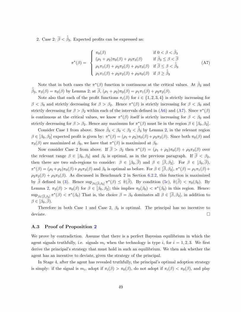
2. Case 2: β <ˆβ3. Expected profits can be expressed as:

π∗(β) =

π0(β) if 0 < β < β3

(ρ1 + ρ2)π0(β) + ρ3π3(β) if β3 ≤ β < β

ρ1π1(β) + ρ2π2(β) + ρ3π3(β) if β ≤ β < ˆβ3

ρ1π1(β) + ρ2π2(β) + ρ3π0(β) if β ≥ ˆβ3

(A7)

Note that in both cases the π∗(β) function is continuous at the critical values. At β3 andˆβ3, π3(β) = π0(β) by Lemma 2; at β, (ρ1 + ρ2)π0(β) = ρ1π1(β) + ρ2π2(β).

Note also that each of the profit functions πi(β) for i ∈ 1, 2, 3, 4 is strictly increasing for

β < β0 and strictly decreasing for β > β2. Hence π∗(β) is strictly increasing for β < β0 and

strictly decreasing for β > β2 within each of the intervals defined in (A6) and (A7). Since π∗(β)

is continuous at the critical values, we know π∗(β) itself is strictly increasing for β < β0 and

strictly decreasing for β > β2. Hence any maximum for π∗(β) must lie in the region β ∈ [β0, β2].

Consider Case 1 from above. Since β3 < β0 < β2 <ˆβ3 by Lemma 2, in the relevant region

β ∈ [β0, β2] expected profit is given by: π∗(β) = (ρ1 + ρ2)π0(β) + ρ3π3(β). Since both π0(β) and

π3(β) are maximized at β0, we have that π∗(β) is maximized at β0.

Now consider Case 2 from above. If β > β2 then π∗(β) = (ρ1 + ρ2)π0(β) + ρ3π3(β) over

the relevant range β ∈ [β0, β2] and β0 is optimal, as in the previous paragraph. If β < β2,

then there are two sub-regions to consider: β ∈ [β0, β) and β ∈ [β, β2]. For β ∈ [β0, β),

π∗(β) = (ρ1 +ρ2)π0(β)+ρ3π3(β) and β0 is optimal as before. For β ∈ [β, β2], π∗(β) = ρ1π1(β)+

ρ2π2(β) + ρ3π3(β). As discussed in Benchmark 2 in Section 6.2.2, this function is maximized

by β defined in (3). Hence supβ∈[β,β2] π∗(β) ≤ π(β). By condition (5c), π(β) < π0(β0). By

Lemma 2, π3(β) > π0(β) for β ∈ [β0, β2]; this implies π0(β0) < π∗(β0) in this region. Hence:

supβ∈[β,β2] π∗(β) < π∗(β0) That is, the choice β = β0 dominates all β ∈ [β, β2], in addition to

β ∈ [β0, β).

Therefore in both Case 1 and Case 2, β0 is optimal. The principal has no incentive to

deviate.

A.3 Proof of Proposition 2

We prove by contradiction. Assume that there is a perfect Bayesian equilibrium in which the

agent signals truthfully, i.e. signals mi when the technology is type i, for i = 1, 2, 3. We first

derive the principal’s strategy that must hold in such an equilibrium. We then ask whether the

agent has an incentive to deviate, given the strategy of the principal.

In Stage 4, after the agent has revealed truthfully, the principal’s optimal adoption strategy

is simply: if the signal is mi, adopt if πi(β) > π0(β), do not adopt if πi(β) < π0(β), and play

49

a possibly mixed strategy if πi(β) = π0(β), where the corresponding ranges of β are given by

Lemmas 1-3.

In Stage 1, There are two cases to consider, depending on the relative magnitudes of the

critical values β2 and β3 defined in Lemmas 1 and 2.

1. Case 1: β3 < β2. Expected profits can be expressed as:

π∗(β) =

π0(β) if 0 < β < β3

(ρ1 + ρ2)π0(β) + ρ3π3(β) if β3 ≤ β < β2

ρ1π0(β) + ρ2π2(β) + ρ3π3(β) if β2 ≤ β < ˆβ3

ρ1π0(β) + ρ2π2(β) + ρ3π0(β) ifˆβ3 ≤ β < β1

ρ1π1(β) + ρ2π2(β) + ρ3π0(β) if β ≥ ˆβ1

(A8)

2. Case 2: β2 < β3. Expected profits can be expressed as:

π∗(β) =

π0(β) if 0 < β < β2

(ρ1 + ρ3)π0(β) + ρ2π2(β) if β2 ≤ β < β3

ρ1π0(β) + ρ2π2(β) + ρ3π3(β) if β3 ≤ β < ˆβ3

ρ1π0(β) + ρ2π2(β) + ρ3π0(β) ifˆβ3 ≤ β < β1

ρ1π1(β) + ρ2π2(β) + ρ3π0(β) if β ≥ ˆβ1

(A9)

As in the proof of Proposition 1, in both cases the π∗(β) function is continuous, since

π3(β) = π0(β) at β3 andˆβ3 by Lemma 2, π2(β) = π0(β) at β2 by Lemma 1, and π1(β) = π0(β)

at β1 by Lemma 3. Also as in the proof of Proposition 1, π∗(β) in strictly increasing for

β ∈ (0, β0) and strictly decreasing for β > β2 since each of the πi(β) functions is increasing and

π∗(β) is continuous. Hence the principal’s optimal β must be in [β0, β2].

Recall that β2 < β0 (Lemma 1)and β3 < β0 < β2 <ˆβ3 (Lemma 1). Hence for any β in

the range [β0, β2], the principal adopts following signals m2 or m3 and does not adopt following

signal m1.

Given this strategy of the principal, the agent has a clear incentive to deviate from truth-

telling. If the technology is type 2, the agent is better off signaling m1 to discourage adoption,

since (refer to (A4)), (β∗s0)2

2 > (β∗s2)2

2 . Hence there is no perfect Bayesian equilibrium under

which the agent reveals truthfully.

A.4 Proof of Proposition 3

It once more suffices to show that there is no profitable deviation for either principal or agent.

50

Under this wage schedule, an agent observing a type 2 technology will not want to deviate

(and signal something other than m2) if the following condition holds:

((β∗∗ + γ∗∗)s2)2

2>

(β∗∗s0)2

2(A10)

where the left-hand side is the agent’s utility if type 2 is adopted, and the right-hand side his

utility under the existing technology (refer to A4). Noting that β∗∗ = β0 and β∗∗ + γ∗∗ = β2

and substituting these values into (2), we have π2(β2) = s22β22−F and π0(β0) = s20β

20 . Condition

(5a) implies π2(β2) > π0(β0) (since π2(β0) is increasing for β ∈ [β0, β2)) and hence (A10). The

agent also does not wish to deviate if he observes the other two types for identical reasons as in

the proof of Proposition 1.

The principal’s next-best strategy is not to pay G and to follow the same strategy as in

Proposition 1.55 The principal will not deviate to this strategy if the following holds:

ρ1π0(β0) + ρ2π2(β2) + ρ3π3(β3)−G > (ρ1 + ρ2)π0(β∗) + ρ3π3(β

∗)

where the left-hand side is the payoff to the strategy of Proposition 3 and the right-hand side

is the payoff to the strategy of Proposition 1. Condition (7) ensures this holds, since β∗ = β3 =

β0.

A.5 Proof of Proposition 4

To prove the proposition, it again suffices to show that there is no profitable deviation for either

principal or agent. First we show there is no incentive for the agent to deviate from his strategy,

holding fixed the principal’s strategy. Suppose the experimenter offers L in Stage 2. If the

technology is of type 1 or 3, the agent has no incentive to deviate, for identical reasons as in

Proposition 1. If the technology is of type 2, the agent signals m2. The agent does not have an

incentive to deviate and signal m1 as this would induce the principal to not adopt which will

make him strictly worse off since U(β0, s2) =β20s

22

2 + L > U(β0, s0) =β20s

20

2 if L >β20(s

20−s22)2 as

assumed. The agent also has no (strict) incentive to deviate and signal m3, since this also induces

adoption and leads to the same payoff as signaling m2. Now suppose that the experimenter does

not offer L in Stage 2. Then the agent has no incentive deviate for the same reasons as in

Proposition 1.

Now we show that there is no incentive for the principal to deviate from her strategy, holding

fixed the agent’s strategy. First, recall that we assume G > ρ2 [π2(β2)− π0(β0)] and that the

principal has a zero probability prior that an experimenter will offer an incentive payment L in

55If the principal does not pay G, the agent’s strategy is the same as Proposition 1 and we showed that thereis no profitable deviation for the principal given the agent’s strategy.

51

Stage 2. Therefore, in Stage 1 the principal is playing the game described in Proposition 1 and

so, as shown in the proof for Proposition 1, she has no incentive to deviate if she offers the wage

contract(α∗ = 0, β∗ = p−c0

2

)since it is part of a perfect Bayesian equilibrium for that game.

Now we turn to the principal’s decision in Stage 4. There are three possible signals by the

agent to consider: If the signal is m1, then the condition for the principal not to deviate can be

written:

π0(β0) ≥ π1(β0)

which is true by Lemma 3. If the signal is m2, then the condition for the principal not to deviate

can be written:

π2(β0) ≥ π0(β0)

where there is no L on the left hand side since we, rather than the principal, pay the lump-sum

bonus. This inequality is true by Lemma 1. If the signal is m3, then the condition for the

principal not to deviate can be written:

π3(β0) ≥ π0(β0)

which is true by Lemma 2.

52

Figure 1: “Buckyball” Design

Notes: Figure shows the standard “buckyball” design. It combines 20 hexagons and 12 pentagons.

Figure 2: U.S. Imports of Inflatable Soccer Balls

010

2030

4050

tota

l im

port

s (f

.o.b

.) in

to U

S (

mil.

200

0 U

S$)

1990 1992 1994 1996 1998 2000 2002 2004 2006 2008 2010 2012

year

Pakistan China

Other

Notes: Figure shows import market share within the United States in HS 10-digit category 9506.62.40.80

(“inflatable soccer balls”). Source: United States customs data.

53

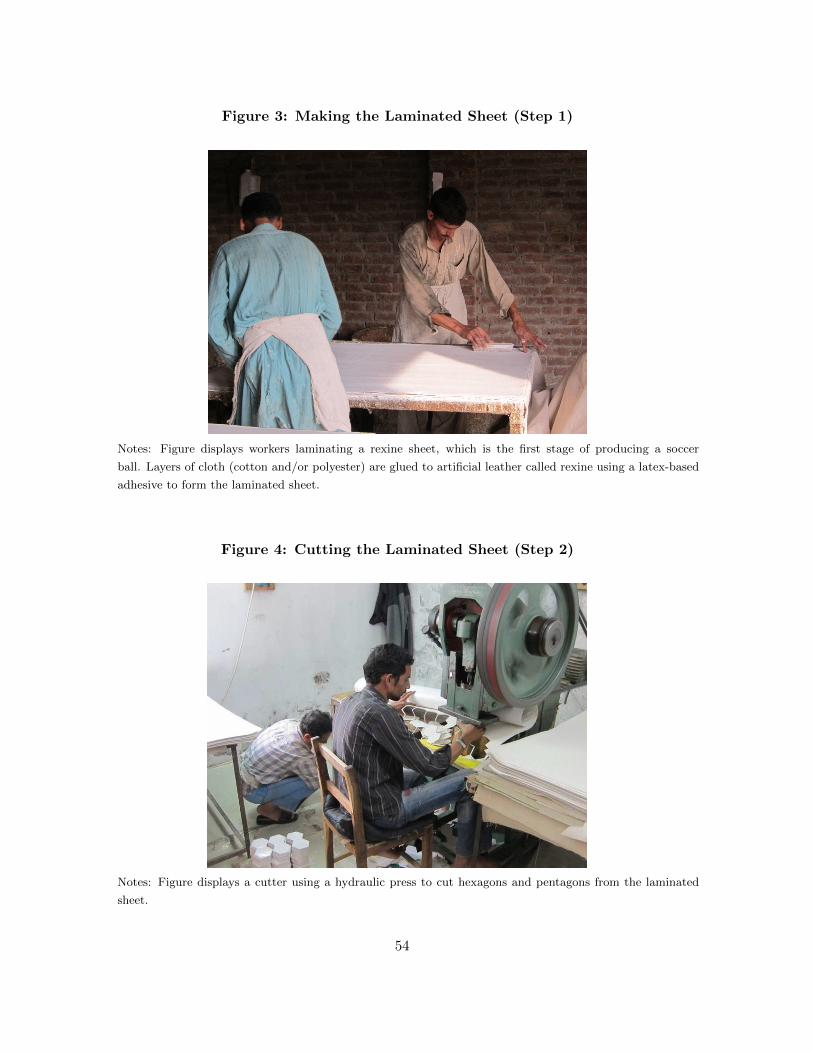
Figure 3: Making the Laminated Sheet (Step 1)

Notes: Figure displays workers laminating a rexine sheet, which is the first stage of producing a soccer

ball. Layers of cloth (cotton and/or polyester) are glued to artificial leather called rexine using a latex-based

adhesive to form the laminated sheet.

Figure 4: Cutting the Laminated Sheet (Step 2)

Notes: Figure displays a cutter using a hydraulic press to cut hexagons and pentagons from the laminated

sheet.

54

Figure 5: Printing the Designs (Step 3)

Notes: Figure displays a worker printing a logo on the pentagon and hexagon panels.

Figure 6: Stitching (Step 4)

Notes: Figure displays a worker stitching a soccer ball. Source: Der Spiegel.

55

Figure 7: Traditional 2-Hexagon and 2-Pentagon Dies

Notes: Figure displays the traditional two-panel hexagon and pentagon dies.

56

Figure 8: Laminated Sheet Wastage from Cutting Hexagons

Notes: Figure displays laminated rexine wastage from cutting hexagons with the traditional two-hexagon die.

Figure 9: Laminated Sheet Wastage from Cutting Pentagons

Notes: Figure displays laminated rexine wastage from cutting pentagons with the traditional two-pentagon

die.

57

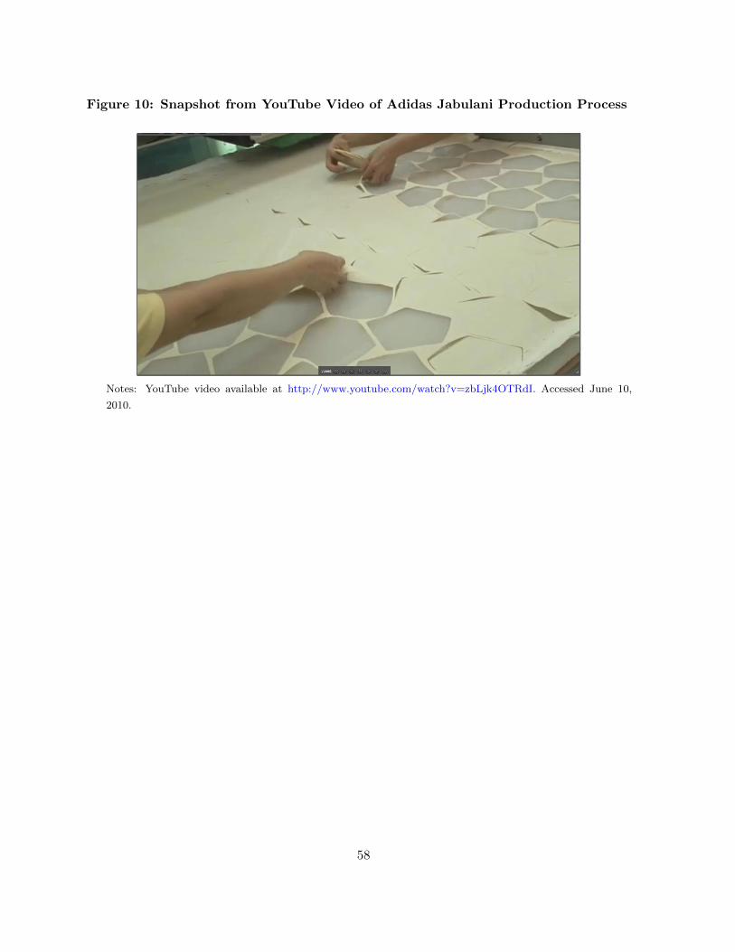
Figure 10: Snapshot from YouTube Video of Adidas Jabulani Production Process

Notes: YouTube video available at http://www.youtube.com/watch?v=zbLjk4OTRdI. Accessed June 10,

2010.

58

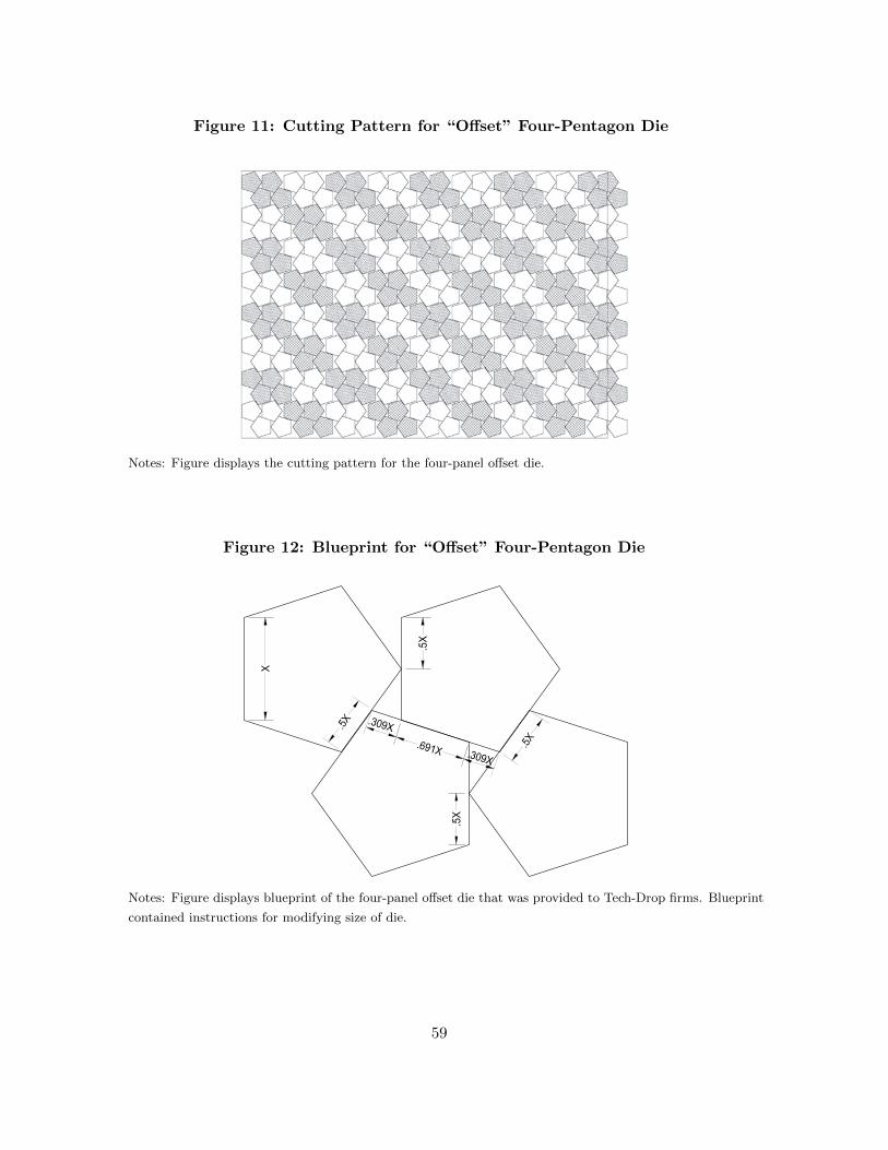
Figure 11: Cutting Pattern for “Offset” Four-Pentagon Die

Notes: Figure displays the cutting pattern for the four-panel offset die.

Figure 12: Blueprint for “Offset” Four-Pentagon Die

Notes: Figure displays blueprint of the four-panel offset die that was provided to Tech-Drop firms. Blueprint

contained instructions for modifying size of die.

59

Figure 13: The “Offset” Four-Pentagon Die

Notes: Figure displays the four-panel offset die that was provided to Tech-Drop firms.

Figure 14: Wikipedia “Pentagon” Page

Notes: Figure displays the Wikipedia “Pentagon” page. Accessed April 29, 2012.

60

Figure 15: Adoption of Offset Dies by Firm Z

010

2030

40

cum

ulat

ive

num

ber

of d

ies

Apr 12 Oct 12 Apr 13 Oct 13 Apr 14

date

61

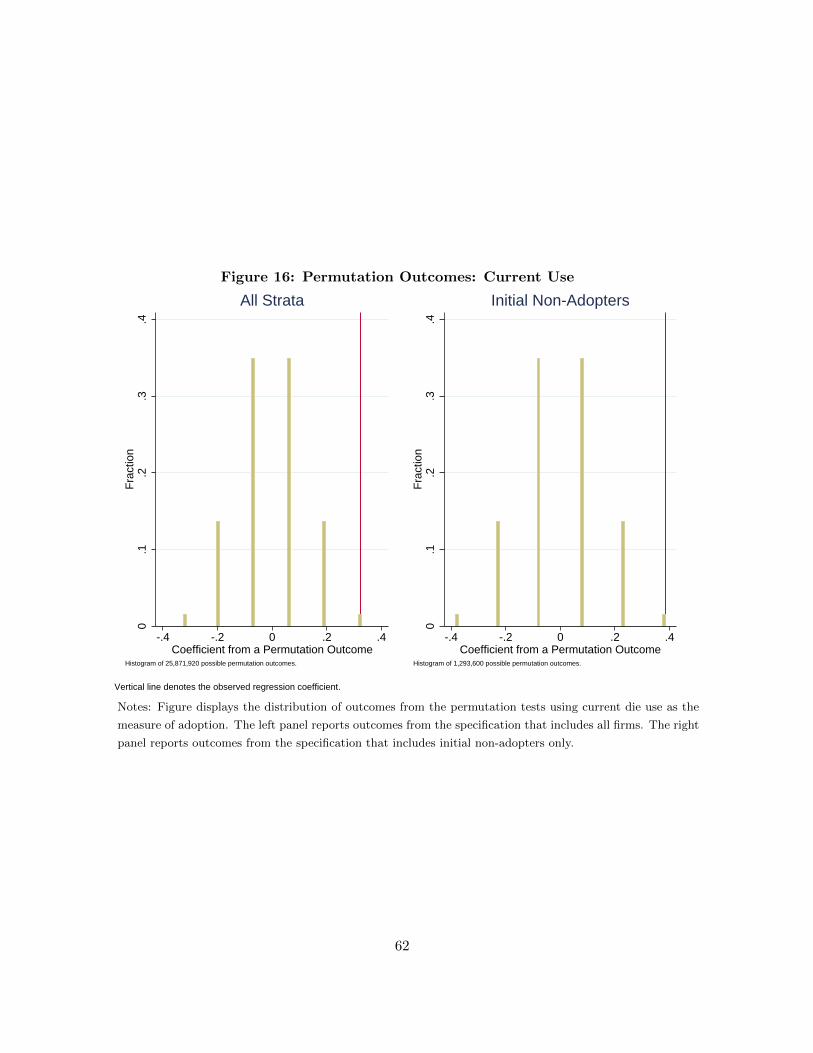
Figure 16: Permutation Outcomes: Current Use

0.1

.2.3

.4F

ract

ion

-.4 -.2 0 .2 .4Coefficient from a Permutation Outcome

Histogram of 25,871,920 possible permutation outcomes.

All Strata

0.1

.2.3

.4F

ract

ion

-.4 -.2 0 .2 .4Coefficient from a Permutation Outcome

Histogram of 1,293,600 possible permutation outcomes.

Initial Non-Adopters

Vertical line denotes the observed regression coefficient.

Notes: Figure displays the distribution of outcomes from the permutation tests using current die use as the

measure of adoption. The left panel reports outcomes from the specification that includes all firms. The right

panel reports outcomes from the specification that includes initial non-adopters only.

62

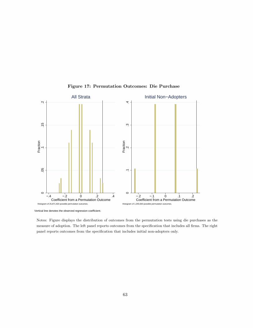
Figure 17: Permutation Outcomes: Die Purchase

0.0

5.1

.15

.2F

ract

ion

−.4 −.2 0 .2 .4Coefficient from a Permutation Outcome

Histogram of 25,871,920 possible permutation outcomes.

All Strata

0.1

.2.3

.4F

ract

ion

−.2 −.1 0 .1 .2Coefficient from a Permutation Outcome

Histogram of 1,293,600 possible permutation outcomes.

Initial Non−Adopters

Vertical line denotes the observed regression coefficient.

Notes: Figure displays the distribution of outcomes from the permutation tests using die purchases as the

measure of adoption. The left panel reports outcomes from the specification that includes all firms. The right

panel reports outcomes from the specification that includes initial non-adopters only.

63

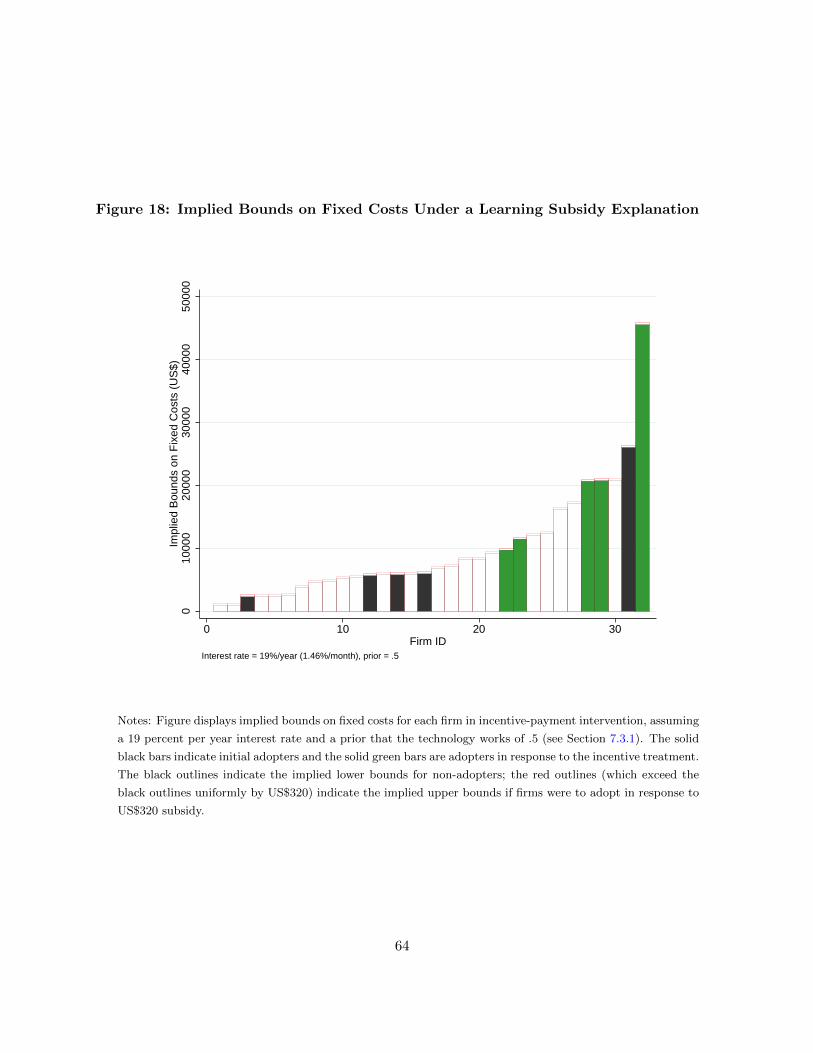
Figure 18: Implied Bounds on Fixed Costs Under a Learning Subsidy Explanation

010

000

2000

030

000

4000

050

000

Impl

ied

Bou

nds

on F

ixed

Cos

ts (

US

$)

0 10 20 30Firm ID

Interest rate = 19%/year (1.46%/month), prior = .5

Notes: Figure displays implied bounds on fixed costs for each firm in incentive-payment intervention, assuming

a 19 percent per year interest rate and a prior that the technology works of .5 (see Section 7.3.1). The solid

black bars indicate initial adopters and the solid green bars are adopters in response to the incentive treatment.

The black outlines indicate the implied lower bounds for non-adopters; the red outlines (which exceed the

black outlines uniformly by US$320) indicate the implied upper bounds if firms were to adopt in response to

US$320 subsidy.

64

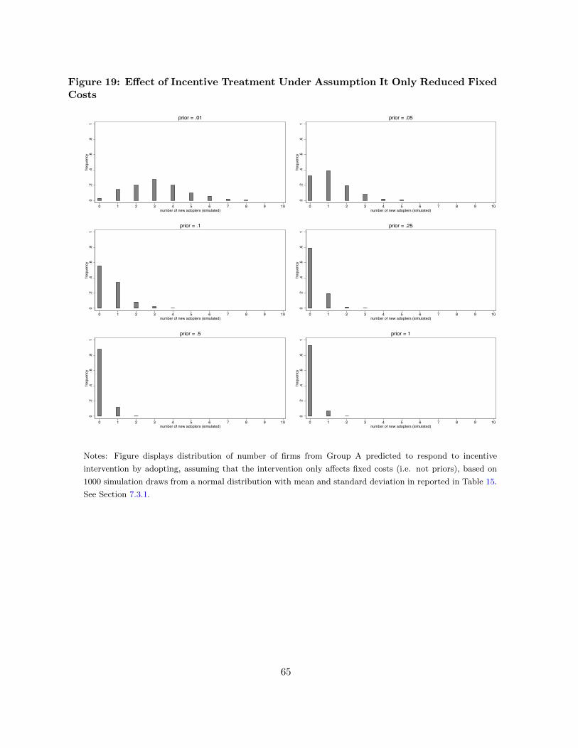
Figure 19: Effect of Incentive Treatment Under Assumption It Only Reduced FixedCosts

0.2

.4.6

.81

freq

uenc

y

0 1 2 3 4 5 6 7 8 9 10number of new adopters (simulated)

prior = .01

0.2

.4.6

.81

freq

uenc

y

0 1 2 3 4 5 6 7 8 9 10number of new adopters (simulated)

prior = .05

0.2

.4.6

.81

freq

uenc

y

0 1 2 3 4 5 6 7 8 9 10number of new adopters (simulated)

prior = .1

0.2

.4.6

.81

freq

uenc

y

0 1 2 3 4 5 6 7 8 9 10number of new adopters (simulated)

prior = .25

0.2

.4.6

.81

freq

uenc

y

0 1 2 3 4 5 6 7 8 9 10number of new adopters (simulated)

prior = .5

0.2

.4.6

.81

freq

uenc

y

0 1 2 3 4 5 6 7 8 9 10number of new adopters (simulated)

prior = 1

Notes: Figure displays distribution of number of firms from Group A predicted to respond to incentive

intervention by adopting, assuming that the intervention only affects fixed costs (i.e. not priors), based on

1000 simulation draws from a normal distribution with mean and standard deviation in reported in Table 15.

See Section 7.3.1.

65

Table 1: Pentagons per Sheet

traditional die offset die

ownerreport

directobs.

ownerreport

directobs.

(1) (2) (3) (4)

size 43.5 257.4 257.7 273.5 277.5(10.4) (6.7) (4.4) (5.3)

size 43.75 256.3 254.4 269.0 272.0(6.2) (9.4) (1.4) (0.0)

size 44 253.8 248.4 280.0 272.5(8.4) (18.7) (0.7)

size 44.25 246.1 262.0 272.0(8.3)

rescaled (to size 44) 253.6 248.3 280.0 272.9(8.5) (11.0) (3.0) (3.9)

N (after rescaling) 274 39 8 10

Notes: Pentagons per sheet rescaled using means for each size in each

column. The N in the final row corresponds to the pooled number of ob-

servations for all die sizes. Standard deviations reported in parentheses.

66

Table 2: Production Costs

Input

Share ofProductionCosts (%)

Input Cost(in Rs)

rexine 19.79 39.68(5.37) (13.87)

cotton/poly cloth 12.32 23.27(4.56) (8.27)

latex 13.94 38.71(10.73) (90.71)

bladder 21.07 42.02(4.87) (14.09)

labor for cutting 0.76 1.47(0.21) (0.30)

labor for stitching 19.67 39.24(5.25) (12.82)

other labor (laminating, washing, packing, matching) 7.32 15.59(4.55) (13.21)

overhead 5.14 10.84(2.05) (6.10)

total 100.00 210.83

N 38 38

Notes: Column 1 reports the mean cost share per ball of each input using the baseline survey. Column 2

reports the cost of each input in Rupees. Total laminated rexine is the sum of the first three components.

The exchange rate is approximately Rs 100 to US$1. Standard deviations reported in parentheses.

67

Table 3: Benefits from Adopting the Offset Die

10th 25th 50th 75th 90th mean

A. Variable cost reductionlaminated rexine waste reduction (%) 4.39 5.19 7.93 8.31 13.43 7.69

(0.46) (0.41) (0.30) (0.05) (1.18) (0.22)laminated rexine as share of cost (%) 34.85 39.87 44.72 51.22 55.44 45.94

(1.14) (0.71) (0.58) (0.44) (0.95) (0.66)variable cost reduction (%) 0.60 0.80 1.10 1.37 1.94 1.17

(0.05) (0.04) (0.03) (0.06) (0.17) (0.04)

B. Variable cost increasecutter wage as share of cost (%) 0.29 0.36 0.45 0.60 0.70 0.48

(0.01) (0.00) (0.01) (0.01) (0.02) (0.01)variable cost increase (%) 0.05 0.06 0.07 0.10 0.12 0.08

(0.00) (0.00) (0.00) (0.00) (0.00) (0.00)C. Net benefitsnet variable cost reduction (%) 0.52 0.72 1.02 1.29 1.87 1.09

(0.05) (0.03) (0.03) (0.06) (0.17) (0.04)% net variable cost/avg % profit rate 5.27 8.10 12.34 19.86 28.98 15.45

(0.42) (0.50) (0.73) (1.21) (2.26) (0.71)total cost savings per month (Rs 000s) 4.46 12.19 49.38 165.21 475.01 174.12

(0.60) (1.24) (5.43) (18.42) (79.89) (18.54)days to recover fixed costs 8.48 15.98 36.61 80.34 193.92 136.94

(0.97) (1.68) (2.93) (6.51) (15.64) (44.54)days to recover fixed costs (no die) 4.40 8.30 19.01 41.71 100.69 71.10

(0.51) (0.87) (1.52) (3.38) (8.12) (23.13)

Notes: Table reports the distribution of benefits from adopting the offset die. The 1st row reports the rexine

waste reduction across firms. The 2nd row reports laminated rexine as a share of unit costs. The 3rd row

reports the variable cost reduction from adopting the offset die, computed as the product of a firm’s rexine

waste reduction, rexine share of cost, and 33 percent (share of pentagons relative to hexagons in total rexine

costs). The 4th row reports the cutter’s wage as a share of unit costs. The 5th row is the variable labor

cost increase percentage from adopting the offset die; this is equal to the product of the cutter share of cost,

a 50 percent increase in cutting time using the offset die relative to traditional die, and 33 percent. The

6th row reports the net variable cost of reduction, which is the difference between a firm’s variable material

cost reduction and its variable labor cost increase. The 7th row reports the total cost savings per month

in Rupees (the exchange rate is approximately Rs 100 to US$1). The 8th row reports the distribution of

the number of days needed to recover all fixed costs of adoption. The 9th row reports the distribution

of the number of days needed to recover fixed costs of adoption, excluding purchasing the die; this final

row is relevant for treatment firms who received the die for free. As noted in the text, the table uses a

hot-deck imputation procedure that replaces a firm’s missing value for a particular cost component with a

draw from the empirical distribution within the firm’s stratum. Since the late responder sample was not

asked rexine share of costs (row 2) at baseline, we draw from the empirical distribution of the full sample

of initial-responder firms. We repeat this process 1,000 times and report the mean and standard deviations

(in parentheses) of each statistic. 68

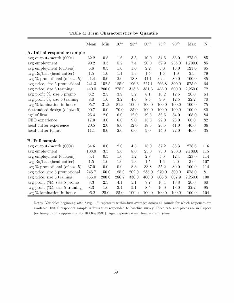
Table 4: Firm Characteristics by Quantile

Mean Min 10th 25th 50th 75th 90th Max N

A. Initial-responder sampleavg output/month (000s) 32.2 0.8 1.6 3.5 10.0 34.6 83.0 275.0 85avg employment 90.2 3.3 5.2 7.4 20.0 52.9 235.0 1,700.0 85avg employment (cutters) 5.8 0.5 1.0 1.0 2.2 5.0 13.0 123.0 85avg Rs/ball (head cutter) 1.5 1.0 1.1 1.3 1.5 1.6 1.9 2.9 79avg % promotional (of size 5) 41.4 0.0 2.0 18.8 41.1 62.4 80.0 100.0 85avg price, size 5 promotional 241.3 152.5 185.0 196.3 227.1 266.8 300.0 575.0 64avg price, size 5 training 440.0 200.0 275.0 313.8 381.3 488.0 600.0 2,250.0 72avg profit %, size 5 promo 8.2 2.5 3.9 5.2 8.1 10.2 12.5 20.0 64avg profit %, size 5 training 8.0 1.6 3.2 4.6 8.5 9.9 12.5 22.2 70avg % lamination in-house 95.7 31.3 81.3 100.0 100.0 100.0 100.0 100.0 75% standard design (of size 5) 90.7 0.0 70.0 85.0 100.0 100.0 100.0 100.0 80age of firm 25.4 2.0 6.0 12.0 19.5 36.5 54.0 108.0 84CEO experience 17.0 3.0 6.0 9.0 15.5 22.0 28.0 66.0 82head cutter experience 20.5 2.0 8.0 12.0 18.5 26.5 41.0 46.0 36head cutter tenure 11.1 0.0 2.0 6.0 9.0 15.0 22.0 46.0 35

B. Full sampleavg output/month (000s) 34.6 0.0 2.0 4.5 15.0 37.2 86.3 278.6 116avg employment 103.9 3.3 5.6 8.0 25.0 75.0 230.0 2,180.0 115avg employment (cutters) 5.4 0.5 1.0 1.2 2.8 5.0 12.4 123.0 114avg Rs/ball (head cutter) 1.5 1.0 1.0 1.3 1.5 1.6 2.0 3.0 107avg % promotional (of size 5) 37.0 0.0 0.0 8.3 33.8 55.2 80.0 100.0 114avg price, size 5 promotional 245.7 150.0 185.0 202.0 235.0 270.0 300.0 575.0 81avg price, size 5 training 465.0 200.0 286.7 330.0 400.0 506.8 667.9 2,250.0 100avg profit (%), size 5 promo 8.3 2.5 4.1 5.1 7.7 10.4 13.8 20.0 80avg profit (%), size 5 training 8.3 1.6 3.4 5.1 8.5 10.0 13.0 22.2 95avg % lamination in-house 96.2 25.0 85.0 100.0 100.0 100.0 100.0 100.0 104

Notes: Variables beginning with “avg. ...” represent within-firm averages across all rounds for which responses are

available. Initial responder sample is firms that responded to baseline survey. Piece rate and prices are in Rupees

(exchange rate is approximately 100 Rs/US$1). Age, experience and tenure are in years.

69

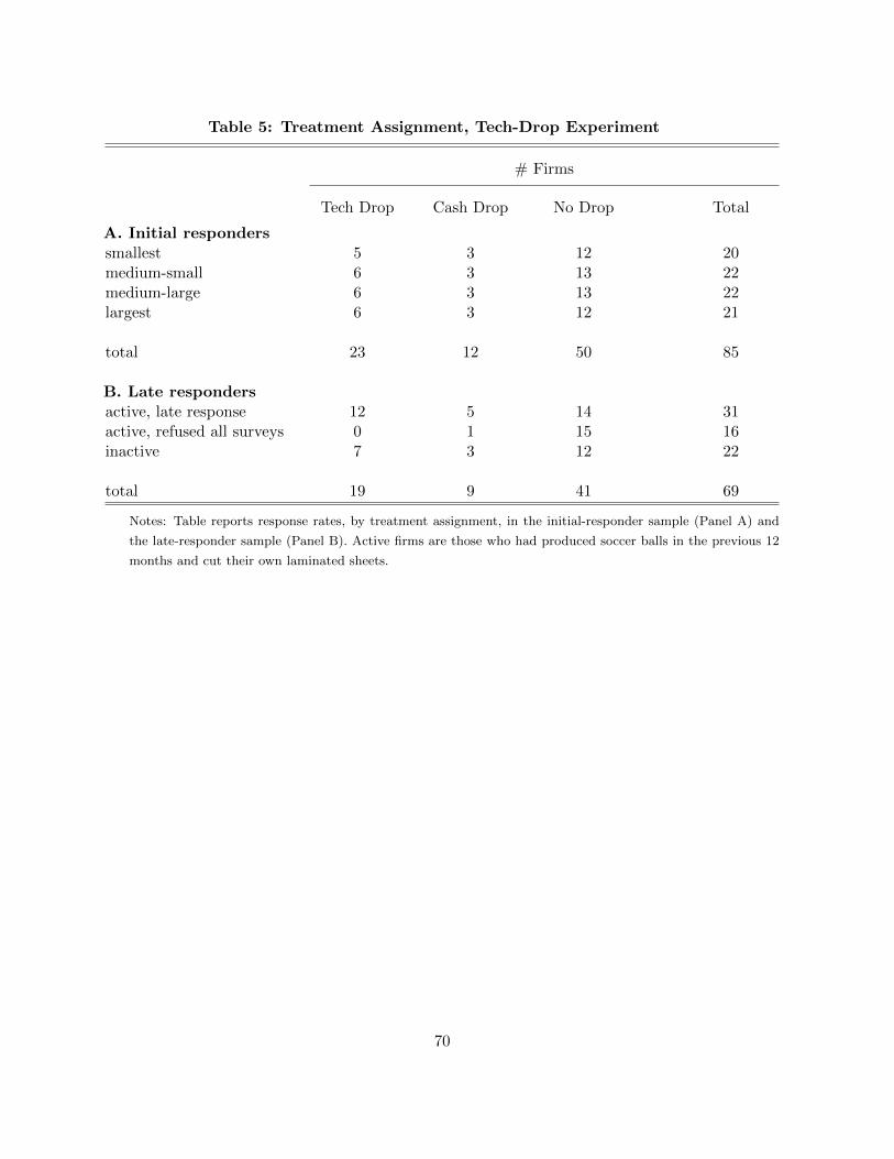
Table 5: Treatment Assignment, Tech-Drop Experiment

# Firms

Tech Drop Cash Drop No Drop Total

A. Initial responderssmallest 5 3 12 20medium-small 6 3 13 22medium-large 6 3 13 22largest 6 3 12 21

total 23 12 50 85

B. Late respondersactive, late response 12 5 14 31active, refused all surveys 0 1 15 16inactive 7 3 12 22

total 19 9 41 69

Notes: Table reports response rates, by treatment assignment, in the initial-responder sample (Panel A) and

the late-responder sample (Panel B). Active firms are those who had produced soccer balls in the previous 12

months and cut their own laminated sheets.

70

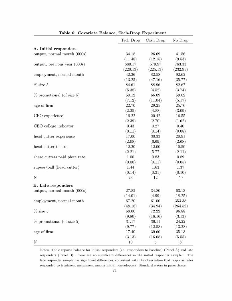
Table 6: Covariate Balance, Tech-Drop Experiment

Tech Drop Cash Drop No Drop

A. Initial respondersoutput, normal month (000s) 34.18 26.69 41.56

(11.48) (12.15) (9.53)output, previous year (000s) 680.17 579.97 763.33

(220.13) (225.13) (232.95)employment, normal month 42.26 82.58 92.62

(13.25) (47.16) (35.77)% size 5 84.61 88.96 82.67

(5.38) (4.52) (3.74)% promotional (of size 5) 50.12 66.09 59.02

(7.12) (11.04) (5.17)age of firm 22.70 29.25 25.76

(2.25) (4.88) (3.09)CEO experience 16.22 20.42 16.55

(2.39) (2.70) (1.62)CEO college indicator 0.43 0.27 0.40

(0.11) (0.14) (0.08)head cutter experience 17.00 30.33 20.91

(2.08) (6.69) (2.68)head cutter tenure 12.20 12.00 10.50

(2.21) (5.77) (2.11)share cutters paid piece rate 1.00 0.83 0.89

(0.00) (0.11) (0.05)rupees/ball (head cutter) 1.44 1.63 1.37

(0.14) (0.21) (0.10)N 23 12 50

B. Late respondersoutput, normal month (000s) 27.85 34.80 63.13

(14.01) (4.99) (18.25)employment, normal month 67.20 61.00 353.38

(48.18) (34.94) (264.52)% size 5 68.00 72.22 96.88

(9.80) (16.16) (3.13)% promotional (of size 5) 31.17 36.11 24.22

(9.77) (12.58) (13.28)age of firm 17.40 39.60 35.13

(3.13) (16.68) (5.55)N 10 5 8

Notes: Table reports balance for initial responders (i.e. responders to baseline) (Panel A) and late

responders (Panel B). There are no significant differences in the initial responder sampler. The

late responder sample has significant differences, consistent with the observation that response rates

responded to treatment assignment among initial non-adopters. Standard errors in parentheses.

71

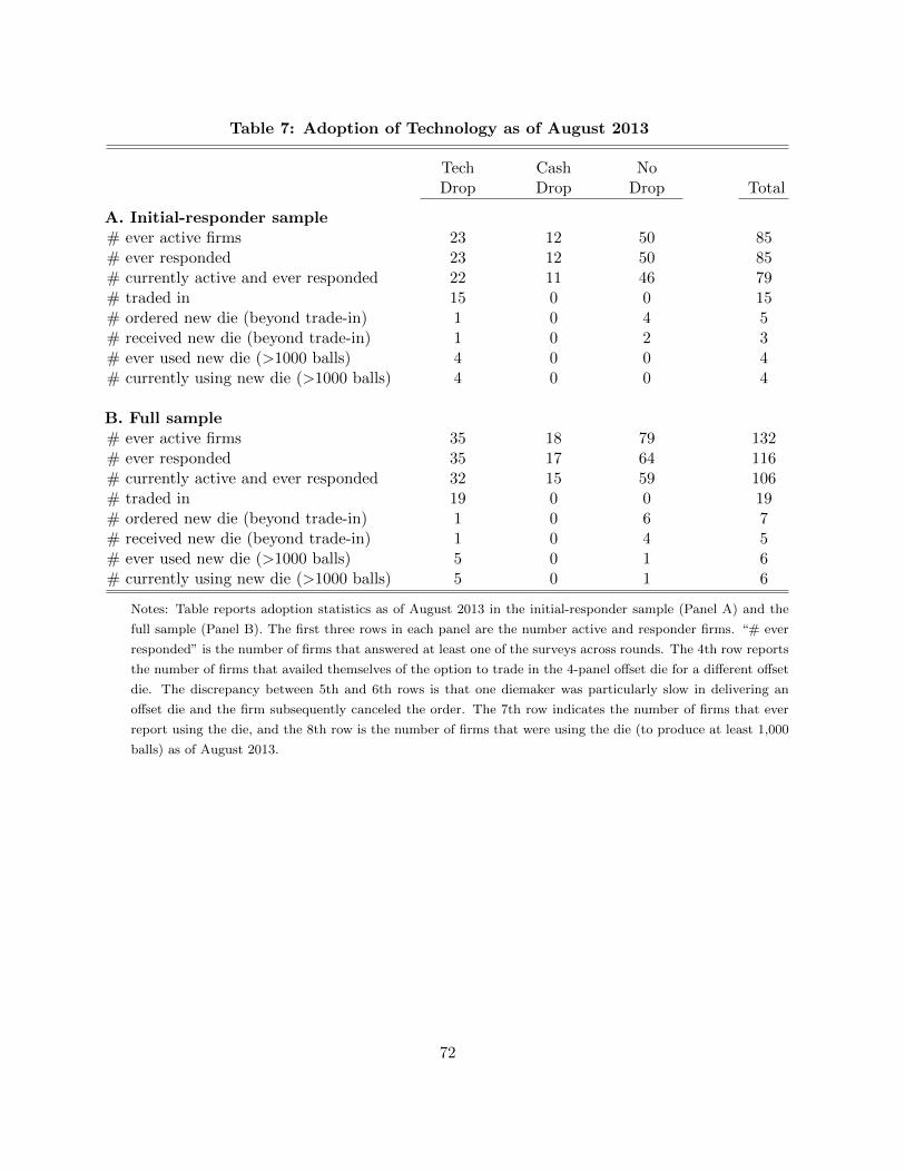
Table 7: Adoption of Technology as of August 2013

TechDrop

CashDrop

NoDrop Total

A. Initial-responder sample# ever active firms 23 12 50 85# ever responded 23 12 50 85# currently active and ever responded 22 11 46 79# traded in 15 0 0 15# ordered new die (beyond trade-in) 1 0 4 5# received new die (beyond trade-in) 1 0 2 3# ever used new die (>1000 balls) 4 0 0 4# currently using new die (>1000 balls) 4 0 0 4

B. Full sample# ever active firms 35 18 79 132# ever responded 35 17 64 116# currently active and ever responded 32 15 59 106# traded in 19 0 0 19# ordered new die (beyond trade-in) 1 0 6 7# received new die (beyond trade-in) 1 0 4 5# ever used new die (>1000 balls) 5 0 1 6# currently using new die (>1000 balls) 5 0 1 6

Notes: Table reports adoption statistics as of August 2013 in the initial-responder sample (Panel A) and the

full sample (Panel B). The first three rows in each panel are the number active and responder firms. “# ever

responded” is the number of firms that answered at least one of the surveys across rounds. The 4th row reports

the number of firms that availed themselves of the option to trade in the 4-panel offset die for a different offset

die. The discrepancy between 5th and 6th rows is that one diemaker was particularly slow in delivering an

offset die and the firm subsequently canceled the order. The 7th row indicates the number of firms that ever

report using the die, and the 8th row is the number of firms that were using the die (to produce at least 1,000

balls) as of August 2013.

72

Tab

le8:

Corr

ela

tes

of

Ad

op

tion

:Scale

&Q

uality

Vari

ab

les

(In

itia

l-R

esp

on

der

Sam

ple

)

Dep

.va

r.:

ind

icat

orfo

rcu

rren

tly

usi

ng

offse

td

ie(1

)(2

)(3

)(4

)(5

)(6

)(7

)(8

)(9

)(1

0)

tech

dro

pgr

oup

0.18

**0.

18**

0.59

0.17

**(0

.08)

(0.0

8)(0

.51)

(0.0

7)ca

shd

rop

gro

up

-0.0

0(0

.02)

log

avg

outp

ut/

mon

th0.

030.

04*

0.03

0.06

(0.0

3)(0

.02)

(0.0

3)(0

.04)

log

avg

outp

ut*

tech

dro

p-0

.04

(0.0

5)sh

are

stan

dar

d(o

fsi

ze5)

-0.3

9-0

.38

-0.4

4(0

.32)

(0.3

3)(0

.27)

log

avg

pri

ce,

size

5tr

ain

ing

-0.0

6-0

.19*

(0.0

5)(0

.11)

avg

shar

ep

rom

oti

on

al

(of

size

5)

-0.1

1-0

.16

(0.0

7)(0

.10)

avg

pro

fit

rate

,si

ze5

trai

nin

g0.

540.

37(0

.64)

(0.6

2)co

nst

ant

0.02

0.02

-0.2

2-0

.29

0.41

0.14

0.40

0.11

0.02

1.14

*(0

.05)

(0.0

5)(0

.22)

(0.1

8)(0

.32)

(0.4

5)(0

.31)

(0.0

7)(0

.05)

(0.6

7)

stra

tum

du

mm

ies

YY

YY

YY

YY

YY

R-s

qu

are

d0.

220.

220.

100.

250.

160.

180.

090.

100.

100.

37N

7979

7979

7474

6879

6663

Note

s:T

able

rep

ort

slinea

rpro

babilit

yre

gre

ssio

ns

of

tech

nolo

gy

adopti

on,

mea

sure

das

curr

ent

use

,on

firm

chara

cter

isti

csfo

rth

ein

itia

l-re

sponder

sam

ple

.V

ari

able

sb

egin

nin

gw

ith

“av

g.

...”

repre

sent

wit

hin

-firm

aver

ages

acr

oss

all

rounds

for

whic

hre

sponse

sare

available

.A

llre

gre

ssio

ns

incl

ude

stra

tum

dum

mie

s.Sig

nifi

cance

:*

.10;

**

.05;

***

0.0

1.

73

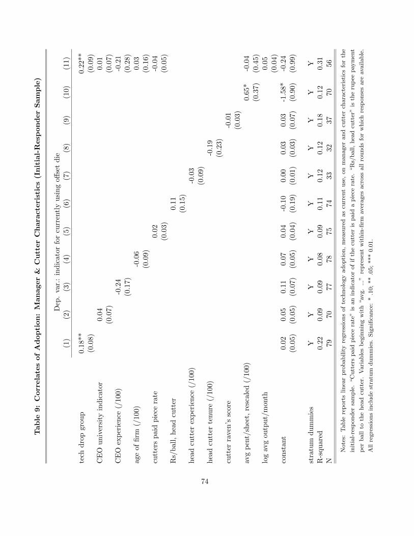
Tab

le9:

Corr

ela

tes

of

Ad

op

tion

:M

an

ager

&C

utt

er

Ch

ara

cte

rist

ics

(In

itia

l-R

esp

on

der

Sam

ple

)

Dep

.va

r.:

ind

icat

orfo

rcu

rren

tly

usi

ng

offse

td

ie(1

)(2

)(3

)(4

)(5

)(6

)(7

)(8

)(9

)(1

0)(1

1)

tech

dro

pgr

oup

0.1

8**

0.22

**(0

.08)

(0.0

9)C

EO

un

iver

sity

ind

icato

r0.

040.

01(0

.07)

(0.0

7)C

EO

exp

erie

nce

(/100)

-0.2

4-0

.21

(0.1

7)(0

.28)

age

of

firm

(/100

)-0

.06

0.03

(0.0

9)(0

.16)

cutt

ers

pai

dp

iece

rate

0.02

-0.0

4(0

.03)

(0.0

5)R

s/b

all

,h

ead

cutt

er0.

11(0

.15)

hea

dcu

tter

exp

erie

nce

(/100)

-0.0

3(0

.09)

hea

dcu

tter

tenu

re(/

100)

-0.1

9(0

.23)

cutt

erra

ven

’ssc

ore

-0.0

1(0

.03)

avg

pen

t/sh

eet,

resc

ale

d(/

100)

0.65

*-0

.04

(0.3

7)(0

.45)

log

avg

ou

tpu

t/m

onth

0.05

(0.0

4)co

nst

ant

0.0

20.

050.

110.

070.

04-0

.10

0.00

0.03

0.03

-1.5

8*-0

.24

(0.0

5)(0

.05)

(0.0

7)(0

.05)

(0.0

4)(0

.19)

(0.0

1)(0

.03)

(0.0

7)(0

.90)

(0.9

9)

stra

tum

du

mm

ies

YY

YY

YY

YY

YY

YR

-squ

ared

0.22

0.09

0.09

0.08

0.09

0.11

0.12

0.12

0.18

0.12

0.31

N79

7077

7875

7433

3237

7056

Note

s:T

able

rep

ort

slinea

rpro

babilit

yre

gre

ssio

ns

of

tech

nolo

gy

adopti

on,

mea

sure

das

curr

ent

use

,on

manager

and

cutt

erch

ara

cter

isti

csfo

rth

e

init

ial-

resp

onder

sam

ple

.“C

utt

ers

paid

pie

cera

te”

isan

indic

ato

rof

ifth

ecu

tter

ispaid

apie

cera

te.

“R

s/ball,

hea

dcu

tter

”is

the

rup

eepay

men

t

per

ball

toth

ehea

dcu

tter

.V

ari

able

sb

egin

nin

gw

ith

“av

g.

...”

repre

sent

wit

hin

-firm

aver

ages

acr

oss

all

rounds

for

whic

hre

sponse

sare

available

.

All

regre

ssio

ns

incl

ude

stra

tum

dum

mie

s.Sig

nifi

cance

:*

.10;

**

.05;

***

0.0

1.

74

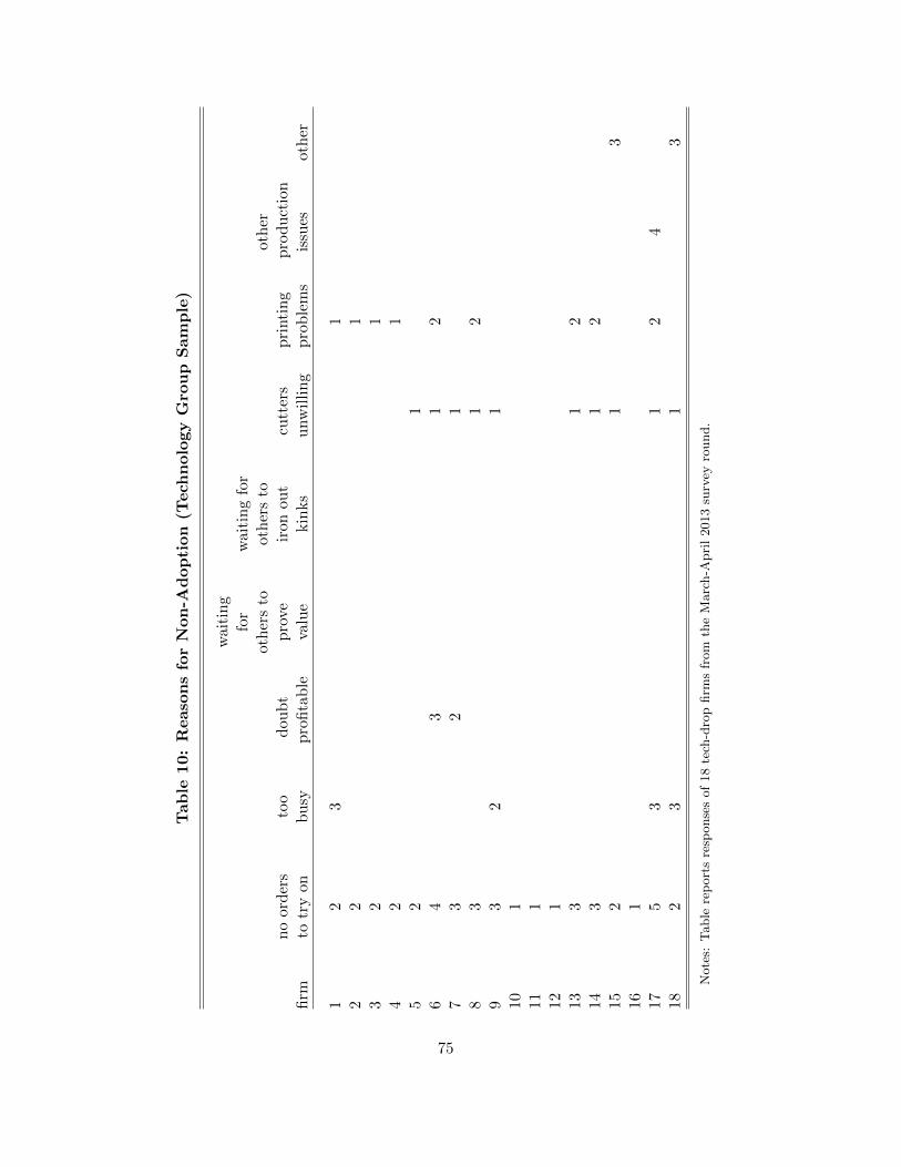
Tab

le10:

Reaso

ns

for

Non

-Ad

op

tion

(Tech

nolo

gy

Gro

up

Sam

ple

)

firm

no

ord

ers

totr

yon

too

bu

syd

oub

tp

rofi

tab

le

wai

tin

gfo

rot

her

sto

pro

veva

lue

wai

tin

gfo

rot

her

sto

iron

out

kin

ks

cutt

ers

unw

illi

ng

pri

nti

ng

pro

ble

ms

oth

erp

rod

uct

ion

issu

esot

her

12

31

22

13

21

42

15

21

64

31

27

32

18

31

29

32

110

111

112

113

31

214

31

215

21

316

117

53

12

418

23

13

Note

s:T

able

rep

ort

sre

sponse

sof

18

tech

-dro

pfirm

sfr

om

the

Marc

h-A

pri

l2013

surv

eyro

und.

75

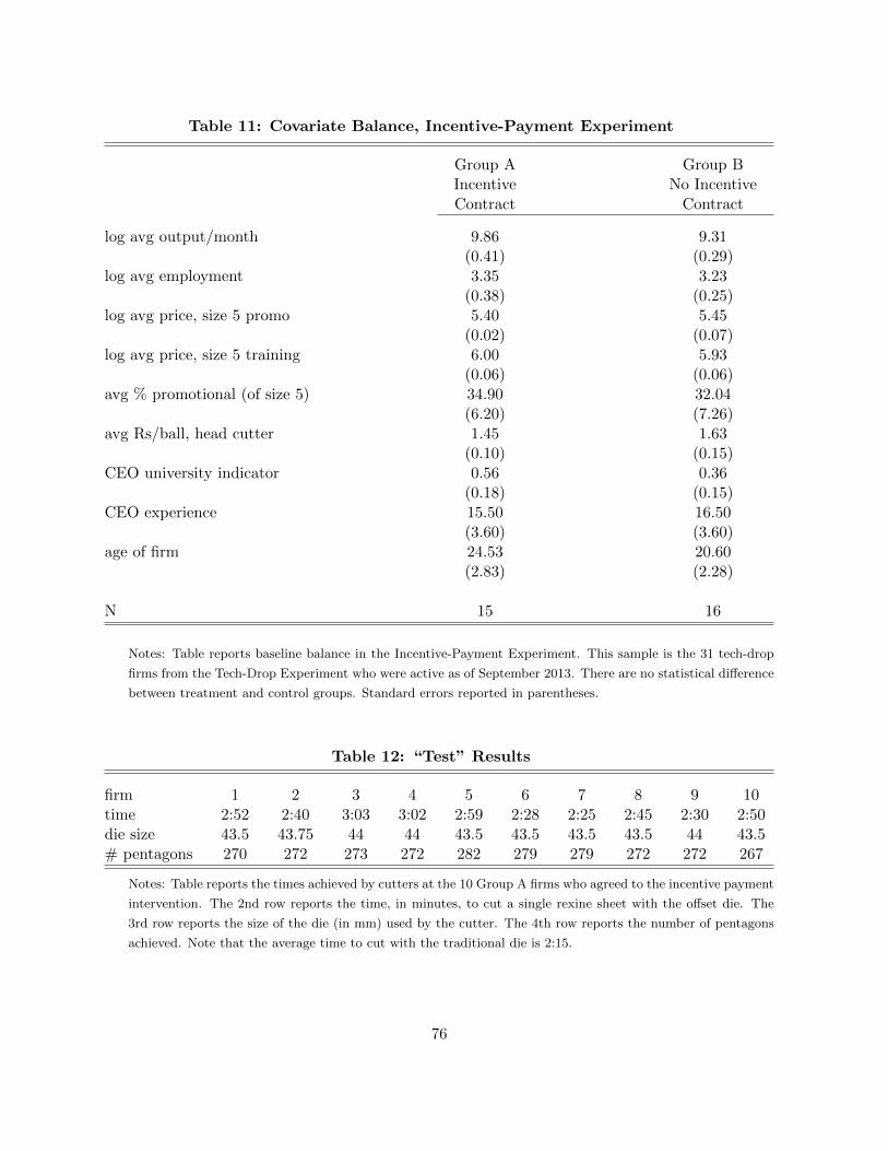
Table 11: Covariate Balance, Incentive-Payment Experiment

Group AIncentiveContract

Group BNo Incentive

Contract

log avg output/month 9.86 9.31(0.41) (0.29)

log avg employment 3.35 3.23(0.38) (0.25)

log avg price, size 5 promo 5.40 5.45(0.02) (0.07)

log avg price, size 5 training 6.00 5.93(0.06) (0.06)

avg % promotional (of size 5) 34.90 32.04(6.20) (7.26)

avg Rs/ball, head cutter 1.45 1.63(0.10) (0.15)

CEO university indicator 0.56 0.36(0.18) (0.15)

CEO experience 15.50 16.50(3.60) (3.60)

age of firm 24.53 20.60(2.83) (2.28)

N 15 16

Notes: Table reports baseline balance in the Incentive-Payment Experiment. This sample is the 31 tech-drop

firms from the Tech-Drop Experiment who were active as of September 2013. There are no statistical difference

between treatment and control groups. Standard errors reported in parentheses.

Table 12: “Test” Results

firm 1 2 3 4 5 6 7 8 9 10time 2:52 2:40 3:03 3:02 2:59 2:28 2:25 2:45 2:30 2:50die size 43.5 43.75 44 44 43.5 43.5 43.5 43.5 44 43.5# pentagons 270 272 273 272 282 279 279 272 272 267

Notes: Table reports the times achieved by cutters at the 10 Group A firms who agreed to the incentive payment

intervention. The 2nd row reports the time, in minutes, to cut a single rexine sheet with the offset die. The

3rd row reports the size of the die (in mm) used by the cutter. The 4th row reports the number of pentagons

achieved. Note that the average time to cut with the traditional die is 2:15.

76

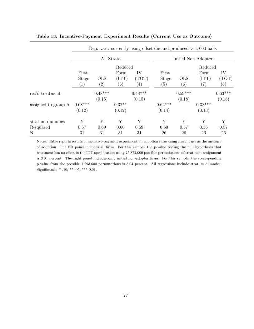
Table 13: Incentive-Payment Experiment Results (Current Use as Outcome)

Dep. var.: currently using offset die and produced > 1, 000 balls

All Strata Initial Non-Adopters

FirstStage OLS

ReducedForm(ITT)

IV(TOT)

FirstStage OLS

ReducedForm(ITT)

IV(TOT)

(1) (2) (3) (4) (5) (6) (7) (8)

rec’d treatment 0.48*** 0.48*** 0.59*** 0.63***(0.15) (0.15) (0.18) (0.18)

assigned to group A 0.68*** 0.32** 0.62*** 0.38***(0.12) (0.12) (0.14) (0.13)

stratum dummies Y Y Y Y Y Y Y YR-squared 0.57 0.69 0.60 0.69 0.50 0.57 0.36 0.57N 31 31 31 31 26 26 26 26

Notes: Table reports results of incentive-payment experiment on adoption rates using current use as the measure

of adoption. The left panel includes all firms. For this sample, the p-value testing the null hypothesis that

treatment has no effect in the ITT specification using 25,872,000 possible permutations of treatment assignment

is 3.04 percent. The right panel includes only initial non-adopter firms. For this sample, the corresponding

p-value from the possible 1,293,600 permutations is 3.04 percent. All regressions include stratum dummies.

Significance: * .10; ** .05; *** 0.01.

77

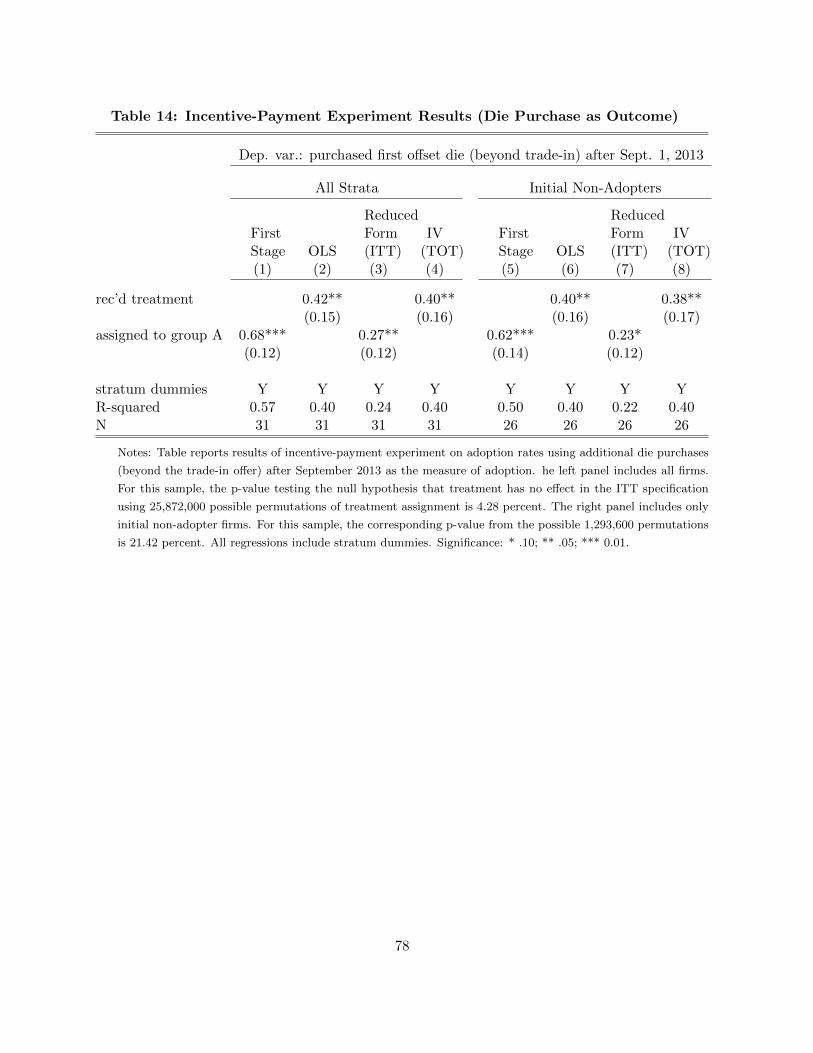
Table 14: Incentive-Payment Experiment Results (Die Purchase as Outcome)

Dep. var.: purchased first offset die (beyond trade-in) after Sept. 1, 2013

All Strata Initial Non-Adopters

FirstStage OLS

ReducedForm(ITT)

IV(TOT)

FirstStage OLS

ReducedForm(ITT)

IV(TOT)

(1) (2) (3) (4) (5) (6) (7) (8)

rec’d treatment 0.42** 0.40** 0.40** 0.38**(0.15) (0.16) (0.16) (0.17)

assigned to group A 0.68*** 0.27** 0.62*** 0.23*(0.12) (0.12) (0.14) (0.12)

stratum dummies Y Y Y Y Y Y Y YR-squared 0.57 0.40 0.24 0.40 0.50 0.40 0.22 0.40N 31 31 31 31 26 26 26 26

Notes: Table reports results of incentive-payment experiment on adoption rates using additional die purchases

(beyond the trade-in offer) after September 2013 as the measure of adoption. he left panel includes all firms.

For this sample, the p-value testing the null hypothesis that treatment has no effect in the ITT specification

using 25,872,000 possible permutations of treatment assignment is 4.28 percent. The right panel includes only

initial non-adopter firms. For this sample, the corresponding p-value from the possible 1,293,600 permutations

is 21.42 percent. All regressions include stratum dummies. Significance: * .10; ** .05; *** 0.01.

78

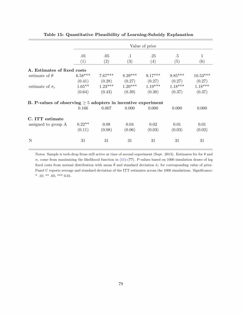
Table 15: Quantitative Plausibility of Learning-Subsidy Explanation

Value of prior

.01 .05 .1 .25 .5 1(1) (2) (3) (4) (5) (6)

A. Estimates of fixed costsestimate of θ 6.58*** 7.67*** 8.29*** 9.17*** 9.85*** 10.53***

(0.41) (0.28) (0.27) (0.27) (0.27) (0.27)estimate of σε 1.65** 1.23*** 1.20*** 1.19*** 1.18*** 1.18***

(0.64) (0.43) (0.39) (0.38) (0.37) (0.37)

B. P-values of observing ≥ 5 adopters in incentive experiment0.166 0.007 0.000 0.000 0.000 0.000

C. ITT estimateassigned to group A 0.22** 0.08 0.04 0.02 0.01 0.01

(0.11) (0.08) (0.06) (0.03) (0.03) (0.02)

N 31 31 31 31 31 31

Notes: Sample is tech-drop firms still active at time of second experiment (Sept. 2013). Estimates for for θ and

σε come from maximizing the likelihood function in (11)-(??). P-values based on 1000 simulation draws of log

fixed costs from normal distribution with mean θ and standard deviation σε for corresponding value of prior.

Panel C reports average and standard deviation of the ITT estimates across the 1000 simulations. Significance:

* .10; ** .05; *** 0.01.

79

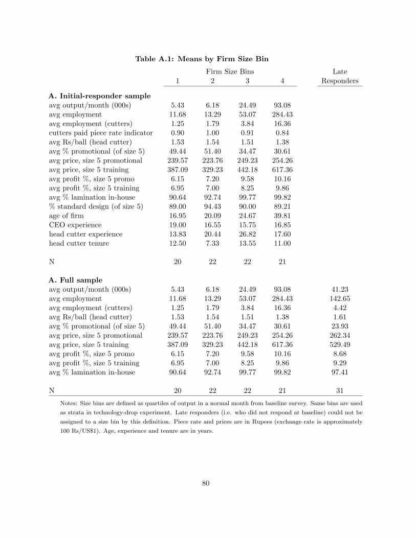
Table A.1: Means by Firm Size Bin

Firm Size Bins Late1 2 3 4 Responders

A. Initial-responder sampleavg output/month (000s) 5.43 6.18 24.49 93.08avg employment 11.68 13.29 53.07 284.43avg employment (cutters) 1.25 1.79 3.84 16.36cutters paid piece rate indicator 0.90 1.00 0.91 0.84avg Rs/ball (head cutter) 1.53 1.54 1.51 1.38avg % promotional (of size 5) 49.44 51.40 34.47 30.61avg price, size 5 promotional 239.57 223.76 249.23 254.26avg price, size 5 training 387.09 329.23 442.18 617.36avg profit %, size 5 promo 6.15 7.20 9.58 10.16avg profit %, size 5 training 6.95 7.00 8.25 9.86avg % lamination in-house 90.64 92.74 99.77 99.82% standard design (of size 5) 89.00 94.43 90.00 89.21age of firm 16.95 20.09 24.67 39.81CEO experience 19.00 16.55 15.75 16.85head cutter experience 13.83 20.44 26.82 17.60head cutter tenure 12.50 7.33 13.55 11.00

N 20 22 22 21

A. Full sampleavg output/month (000s) 5.43 6.18 24.49 93.08 41.23avg employment 11.68 13.29 53.07 284.43 142.65avg employment (cutters) 1.25 1.79 3.84 16.36 4.42avg Rs/ball (head cutter) 1.53 1.54 1.51 1.38 1.61avg % promotional (of size 5) 49.44 51.40 34.47 30.61 23.93avg price, size 5 promotional 239.57 223.76 249.23 254.26 262.34avg price, size 5 training 387.09 329.23 442.18 617.36 529.49avg profit %, size 5 promo 6.15 7.20 9.58 10.16 8.68avg profit %, size 5 training 6.95 7.00 8.25 9.86 9.29avg % lamination in-house 90.64 92.74 99.77 99.82 97.41

N 20 22 22 21 31

Notes: Size bins are defined as quartiles of output in a normal month from baseline survey. Same bins are used

as strata in technology-drop experiment. Late responders (i.e. who did not respond at baseline) could not be

assigned to a size bin by this definition. Piece rate and prices are in Rupees (exchange rate is approximately

100 Rs/US$1). Age, experience and tenure are in years.

80