Orientation Bandwidth: the Effect of Spatial and Temporal ...psych.cf.ac.uk/home2/snowden/1992_VisionRes_Snowden.pdf · no orientation specific adaptation-implying that the ... bandwidth

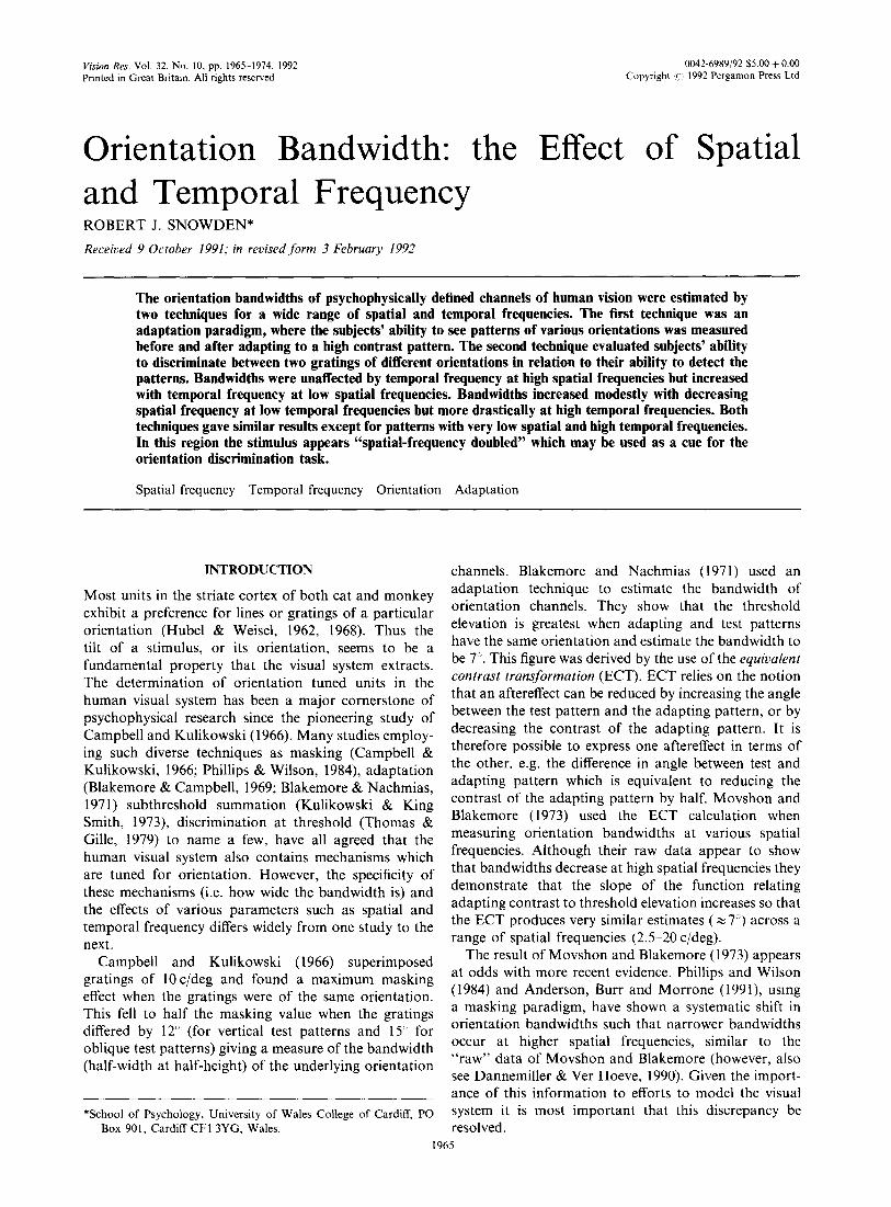
Vision Res. Vol. 32, No. 10, pp. 1965-1974, 1992 Printed in Great Britain. All rights reserved

0042-6989/92 $5.00 + 0.00 Copyright ‘(_! 1992 Pergamon Press Ltd

Orientation Bandwidth: the and Temporal Frequency ROBERT J. SNOWDEN*

Received 9 October 1991; in revised form 3 February 1992

Effect of Spatial

The orientation bandwidths of psychophysically defined channels of human vision were estimated by two techniques for a wide range of spatial and temporal frequencies. The first technique was an adaptation paradigm, where the subjects’ ability to see patterns of various orientations was measured before and after adapting to a high contrast pattern. The second technique evaluated subjects’ ability to discriminate between two gratings of different orientations in relation to their ability to detect the patterns. Bandwidths were unaffected by temporal frequency at high spatial frequencies but increased with temporal frequency at low spatial frequencies. Bandwidths increased modestly with decreasing spatial frequency at low temporal frequencies but more drastically at high temporal frequencies. Both techniques gave similar results except for patterns with very low spatial and high temporal frequencies. In this region the stimulus appears “spatial-frequency doubled” which may be used as a cue for the orientation discrimination task.

Spatial frequency Temporal frequency Orientation Adaptation

INTRODUCTION

Most units in the striate cortex of both cat and monkey exhibit a preference for lines or gratings of a particular orientation (Hubel & Weisel, 1962, 1968). Thus the tilt of a stimulus, or its orientation, seems to be a fundamental property that the visual system extracts. The determination of orientation tuned units in the

human visual system has been a major cornerstone of psychophysical research since the pioneering study of

Campbell and Kulikowski (1966). Many studies employ- ing such diverse techniques as masking (Campbell & Kulikowski, 1966; Phillips & Wilson, 1984) adaptation (Blakemore & Campbell, 1969; Blakemore & Nachmias, 1971) subthreshold summation (Kulikowski & King Smith, 1973) discrimination at threshold (Thomas & Gille, 1979) to name a few, have all agreed that the human visual system also contains mechanisms which are tuned for orientation. However, the specificity of these mechanisms (i.e. how wide the bandwidth is) and the effects of various parameters such as spatial and temporal frequency differs widely from one study to the next.

Campbell and Kulikowski (1966) superimposed gratings of 10 c/deg and found a maximum masking effect when the gratings were of the same orientation. This fell to half the masking value when the gratings differed by 12” (for vertical test patterns and 15” for oblique test patterns) giving a measure of the bandwidth (half-width at half-height) of the underlying orientation

*School of Psychology, University of Wales College of Cardiff, PO Box 901, Cardiff CFI 3YG, Wales.

channels. Blakemore and Nachmias (1971) used an adaptation technique to estimate the bandwidth of orientation channels. They show that the threshold elevation is greatest when adapting and test patterns have the same orientation and estimate the bandwidth to be 7”. This figure was derived by the use of the equivalent

contrast transformation (ECT). ECT relies on the notion that an aftereffect can be reduced by increasing the angle between the test pattern and the adapting pattern, or by decreasing the contrast of the adapting pattern. It is therefore possible to express one aftereffect in terms of the other, e.g. the difference in angle between test and adapting pattern which is equivalent to reducing the contrast of the adapting pattern by half. Movshon and Blakemore (1973) used the ECT calculation when measuring orientation bandwidths at various spatial frequencies. Although their raw data appear to show that bandwidths decrease at high spatial frequencies they demonstrate that the slope of the function relating adapting contrast to threshold elevation increases so that the ECT produces very similar estimates ( z 7”) across a

range of spatial frequencies (2.5-20 c/deg). The result of Movshon and Blakemore (1973) appears

at odds with more recent evidence. Phillips and Wilson (1984) and Anderson, Burr and Morrone (1991), using a masking paradigm, have shown a systematic shift in orientation bandwidths such that narrower bandwidths occur at higher spatial frequencies, similar to the “raw” data of Movshon and Blakemore (however, also see Dannemiller & Ver Hoeve, 1990). Given the import- ance of this information to efforts to model the visual system it is most important that this discrepancy be resolved.

1965

1966 ROBERT J. SNOWDEN

A second point to note from the data of Phillips and Wilson (1984) is that orientation bandwidths were similar for both a “sustained” presentation (a stationary stimulus presented within a Gaussian time window) and a “transient” presentation (8 Hz square wave). This seems in direct conflict with the findings of two other studies. Sharpe and Tolhurst (1973) estimated orientation bandwidths, using adaptation and the ECT, for both stationary gratings and gratings which were tem- porally modulated at 5 Hz (modulation was achieved by either drifting the gratings or flashing them on and off). They found that the bandwidth increased from 7” to around 12” when the temporal modulation was added and suggest that this difference reflects the workings of two types of channel: “movement analysers and form analysers” (more commonly termed the transient and sustained mechanisms e.g. Legge, 1978). Kelly and Burbeck (1987) have further studied the orientation properties of the transient mechanism using an adaptation paradigm. They show that in the region most likely to be subserved by the transient mechanism (low spatial frequency, high temporal frequency) there is no orientation specific adaptation-implying that the mechanism which adapts is isotropic with respect to orientation.

These studies therefore appear contradictory, one suggesting no effect of temporal frequency (masking: Phillips & Wilson, 1984), one suggesting a relatively small effect (adaptation and ECT: Sharpe & Tolhurst, 1973) and others suggesting an extreme effect (adaptation: Kelly & Burbeck, 1987; for masking data see also But-beck & Kelly, 1981).

Given the widespread disagreement about the effects of spatial and temporal frequency on orientation tuning I have attempted to estimate orientation tuning across a wide range of spatial and temporal frequencies. Two types of measurements have been made. First, bandwidths were estimated using an adaptation paradigm, where the threshold for seeing patterns of various orientations is compared before and after viewing a high contrast pattern of a particular orientation. This technique is presumed to proceed by activating channels closely tuned to the adapting orientation. These channels may either become fatigued by this activity, or cause inhibition of similarly tuned channels whose effects persist for some time after the adapting stimulus is removed. Either way they are desensitised for some period of time after the adapting pattern is removed. By measuring the spread of this desensitisation across orientation a measure of the bandwidth is obtained.

The “bandwidth” estimated by this technique still needs some interpretation. For instance, is the bandwidth estimated at one adapting contrast the same as that estimated at another adapting contrast, and is it fair to compare a bandwidth measured at one spatial frequency with that of another measured at a different spatial frequency? One way of dealing with these prob- lems was the introduction of the ECT (Blakemore & Nachmias, 1971). To recap, the ECT relies on the fact that (a) aftereffects reduce as the contrast of the adapting

pattern is decreased and (b) aftereffects decrease as the difference (in the case of orientation tuning this would be the angle) between the test and adapting patterns increases. In other words the effect of halving the adapting contrast can be expressed in terms of the angle required to produce the same reduction in the effect. Hence if changing the contrast from 40 to 20% is equivalent to a difference in adapt and test of IO-, then changing the adapting contrast from 20 to 10% should also be equivalent to a change of IO”. This will be so if the function relating adapting contrast to threshold elevation has the same slope no matter what the difference in angle between the test and adapting patterns. lf, however, these functions have different slopes then the angle needed to produce the equivalent change in adapting contrast from 40 to 20% will be different from that needed to produce the equivalent change from 20 to 10%. Therefore the measured orientation bandwidth will vary depending on the adapting contrast (for a quantitative model see Snowden, 1991). Under these conditions where the slope changes, Snowden (199 1) has shown that the tuning curves measured at different adapting contrasts are merely scaled versions of one another and thus the bandwidth (measured by the standard deviation of the best fitting Gaussian) remains constant.

ECT was introduced as it seemed inappropriate to measure spatial frequency bandwidths at the same adapting contrast for different spatial frequencies. For some (medium) spatial frequencies this might be well above threshold contrast, whereas for others (particu- larly high spatial frequencies) this same contrast might be quite close to threshold. The “change of slope” model (Snowden, 1991) neatly sidesteps this problem as the bandwidths are predicted to be the same at all adapting contrasts, hence it is a convenient way to compare bandwidths across differing stimulus conditions. In this paper this principle is used to measure orientation bandwidths for a wide range of spatial and temporal frequencies.

The arguments presented in the previous paragraphs have focused upon whether the slope of the threshold elevation function is the same for all differences between adapting and test patterns, or whether it systematically becomes less steep as the angle between the test and adapting patterns increases. While this would seem to be easily resolved by an experiment, those who have tried have produced contradictory reports. In the domain of the specificity of spatial frequency adaptation Stromeyer, Klein and Sternheim (1977) and Swift and Smith (1982) produce data which strongly indicate that the slopes do not change, while Dealy and Tolhurst (1974) and Georgeson and Harris (1984) produce data which indicate an equally convincing change in slope. Likewise in the domain of orientation specific adaptation the data of Ross and Speed (1991) indicate no change in slope, while a systematic study by Snowden (1991) shows a change in slope. The reasons for these discrepancies is still far from clear (for a discussion see Georgeson & Harris, 1984). The data reported here all

ORIENTATION BANDWIDTH 1967

stem from equipment, stimuli and techniques which are essentially the same as that which produced the data

reported in Snowden (1991). In that study it was clearly

shown that the slopes relating threshold elevation to adapting contrast reduced as the difference in angle between the test and adapting pattern increased. Thus, as explained above, bandwidths can be compared across spatial frequencies without any further transformations.

The second technique used to estimate bandwidth is that of discriminating the orientation of the test stimulus near its detection threshold. This technique rests on the

notion that a stimulus at threshold activates only one channel. If stimuli are so similar that at threshold they will activate the same channel they will be indistinguish-

able at threshold, whereas if they are sufficiently different as to activate different channels at threshold they will be distinguishable. This technique therefore makes assumptions about channels being “labelled” as well as on the spacing of these channels (see Graham, 1989).

This paper therefore aims to chart the orientation

bandwidth across the spatio-temporal domain using, and comparing, two quite different measurement techniques. I show that (a) orientation bandwidths are dependent upon both the spatial and temporal aspects of the stimuli (b) that the changes described in (a) are similar for both techniques except in the region of low spatial and high temporal frequencies.

METHODS

Equipment

Grating stimuli were generated using a VSG2/1 (Cam- bridge Research Systems) graphics board housed in a PC, and were displayed on a Joyce scope (P4 phosphor). The luminance values fed to the screen were gamma corrected so that the screen was linear up to 90% contrast. The screen was refreshed at 100 Hz in order to faithfully represent the highest temporal frequencies used in this study (24 Hz). The orientation of the pattern

was achieved by rotating the coil within the Joyce scope via an analogue output under computer control. As it takes the coil a longer time to travel greater angles the screen was set to zero contrast for 200 msec while the coil rotated. This time allowed for complete rotation at even the greatest rotations (90”) before a new stimulus was presented. One problem encountered was that the rotation of the coil was audible to the subject and gave an approximate clue to how far the screen had rotated (though no clue as to which direction). This auditory cue could help a subject in looking for a specific orientation. Since the effect was present both before and after adaptation it should cancel out. For the discrimination task the noise may give an indication of how different the orientation is as compared to horizontal, but gives no clue as to the direction (clockwise or anticlockwise) which is the decision the subject must take. The screen was covered by a white mask save for a circular aperture of 8 cm dia, which from the normal viewing distance of 114 cm subtended 4 deg. Subjects responses were

collected by the computer via the “mouse” buttons. The

data was then analysed off-line via software running on

a Apple Macintosh computer.

Stimuli

Sinewave gratings were used throughout the study. The spatial frequency, temporal frequency (sinewave counterphase), contrast and orientation were all con- trolled by the computer. The mean luminance of all patterns was 200 cd/m2. The gratings were presented within a circular aperture which subtended 4 deg for most stimuli. For the lowest spatial frequencies (0.2 and 0.3 c/deg) this would have meant that there would only

be around 1 cycle of the grating. The results presented here were therefore gathered by viewing the same grating as for the 1 c/deg but altering the viewing distance appropriately (23 and 34 cm), and hence changing the

field size (20 and 13.3 deg). All stimuli were ramped on and off (the ramp sections were of 200 msec duration and contrast increased and decreased linearly) to avoid temporal transients which could seriously affect the results.

Thus a test pattern of “500 msec duration” was actually presented for 900msec, with the pattern being at full contrast for 500 msec. A small mark was made in the centre of the screen to aid fixation.

Subjects

In total three subjects participated in these experiments, the author and two naive subjects, though not all subjects did all the conditions. All viewing was binocular with natural pupils. Subjects were two females (age 19

and 20) and the author (male age 27). All had normal acuity without correction.

EXPERIMENT l-ORIENTATION TUNING AS A FUNCTION OF SPATIAL AND TEMPORAL

FREQUENCY MEASURED BY AN ADAPTATION PARADIGM

Method

Procedure. Subjects viewed the horizontal adapting pattern for 40 set and then went into a test-readapt cycle. The test pattern was viewed for 500 msec

(900 msec total) and then the adapting pattern reap- peared for 4000 msec (4400 msec total). The test pattern was coincident with a warning tone from the computer. The subject indicated whether the test pattern had been seen by pressing one of two buttons (yes/no decision). The contrast of the test pattern was varied from trial to trial according to a modified QUEST procedure (Watson & Pelli, 1983) designed to track contrast at which the subject reported seeing the pattern on 63.2% of trials. On any given block of trials typically six QUESTS were randomly interleaved. These six QUESTS corresponded to differences in orientation between the test and adapting patterns of 0, 15, 30, 45, 60 and 90’. Each QUEST was run until 32 trials had been completed. The contrast of the adapting pattern was 60%. In addition to this a baseline measure was also needed in order to judge the amount of adaptation. This


baseline was achieved by the same methods as above save that the adapting contrast was set to zero.

Analysis of results (adaptation experiments). The data relating probability “yes” was fitted by a Weibull function of the form:

P = 1 -exp{-[lOr\/?/20*(cO/cl)]} (1)

(where P is the probability of a correct response, CO the test contrast, and /? and c 1 the parameters governing the slope and position of the function respectively) via least squares regression. Both the slope and threshold parameters were free to vary. The difference between thresholds before and after adaptation was calculated (indB) and this was then plotted as a function of the difference in orientation between adapting and testing patterns. The results followed those found by previous researchers (e.g. Blakemore & Nachmias, 1971) in that the amount of adaptation fell as the difference between test and adapting pattern increased. In order to quantify this rate of fall a Gaussian function of the form:

threshold elevation = rl . exp[-0.5 . (02/a2)] (2)

(where r] and g are the height and standard deviation of the Gaussian, and 8 is the difference in angle between the test and adapting pattern) was fit to the data. The Gaussian was chosen because it does not depend upon assumptions about which points are to be used in the analysis, and is therefore very convenient. I found it to be a good fit to most of the data (average r = 0.97) with a small but systematic underestimation of the data point at 0” difference. In other words it underestimates the “peakedness” of the function. This was found right across the spatio-temporal range and thus has little effect upon the main points of this paper.

Results

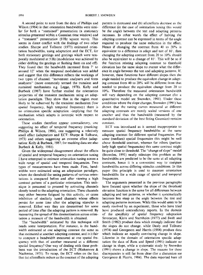
Examples of the tuning curves for one subject can be seen in Fig. 1. The experimental data points were only collected for positive differences (clockwise) but these data points have been simply reflected to produce the whole tuning curve. Threshold elevation is the difference (in dB) between the adapted and unadapted thresholds.

-50 Orienla&n (deg)

50 100

FIGURE 1. The threshold elevation (difference between the threshold before and after adaptation) is plotted as a function of the difference in angle between the test and the adapting pattern. Data were collected for clockwise differences (positive values) but have simply been reflected to show the full curve. The open circles are for a pattern of 1 c/deg flickering at 4 Hz, the solid circles are for 0.3 cjdeg, 4 Hz and the open squares for 1 c/deg, 24 Hz. The curves represent the best

fitting Gaussian functions.

_. RS

g 60. f. 0 40 b 5 m

20 -

0-l 7

.1 1 10

Spatial Frequency (c/deg)

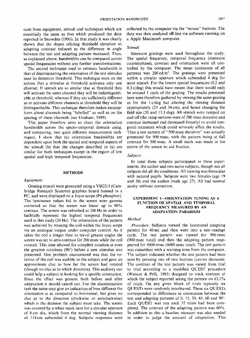
FIGURE 2. The standard deviation of the best fitting Gaussian (termed the bandwidth) is plotted as a function of spatial frequency for two observers JO and RS. Patterns were flickered at 0.5 Hz (solid

circles), 4 Hz (open circles) and 24 Hz (crosses).

The curves are the best fitting Gaussian functions to the data points. The tuning curve is most narrow for the case of 1 c/deg flickering at 4 Hz (open circles) and increased with a decrease in spatial frequency (solid circles) or an increase in temporal frequency (open squares). Data of this kind were gathered for a range of spatial and temporal frequencies and the standard deviation of the best-fitting Gaussian (hereafter termed the bandwidth) is plotted as a function of spatial frequency in Fig. 2, and as a function of temporal frequency in Fig. 3.

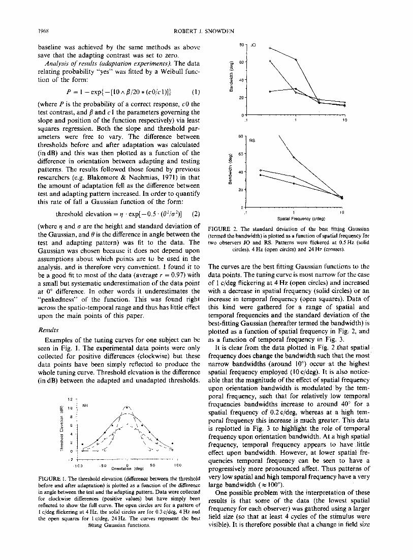
It is clear from the data plotted in Fig. 2 that spatial frequency does change the bandwidth such that the most narrow bandwidths (around loo) occur at the highest spatial frequency employed (10 c/deg). It is also notice- able that the magnitude of the effect of spatial frequency upon orientation bandwidth is modulated by the temporal frequency, such that for relatively low temporal frequencies bandwidths increase to around 40” for a spatial frequency of 0.2 c/deg, whereas at a high temporal frequency this increase is much greater. This data is replotted in Fig. 3 to highlight the role of temporal frequency upon orientation bandwidth. At a high spatial frequency, temporal frequency appears to have little effect upon bandwidth. However, at lower spatial frequencies temporal frequency can be seen to have a progressively more pronounced affect. Thus patterns of very low spatial and high temporal frequency have a very large bandwidth ( RS 100’).

One possible problem with the interpretation of these results is that some of the data (the lowest spatial frequency for each observer) was gathered using a larger field size (so that at least 4 cycles of the stimulus were visible). It is therefore possible that a change in field size


I - 01’_

1 1 10 100

Temporal Frequency (Hz)

FIGURE 3. As for Fig. 2 but as a function of temporal frequency.

Stimuli had a spatial frequency of 10 c/deg (crosses), 3 c/deg (squares),

1 c/deg (open circles), 0.3 c/deg (solid circles-JO) or 0.2 c/deg (solid

circles-RS).

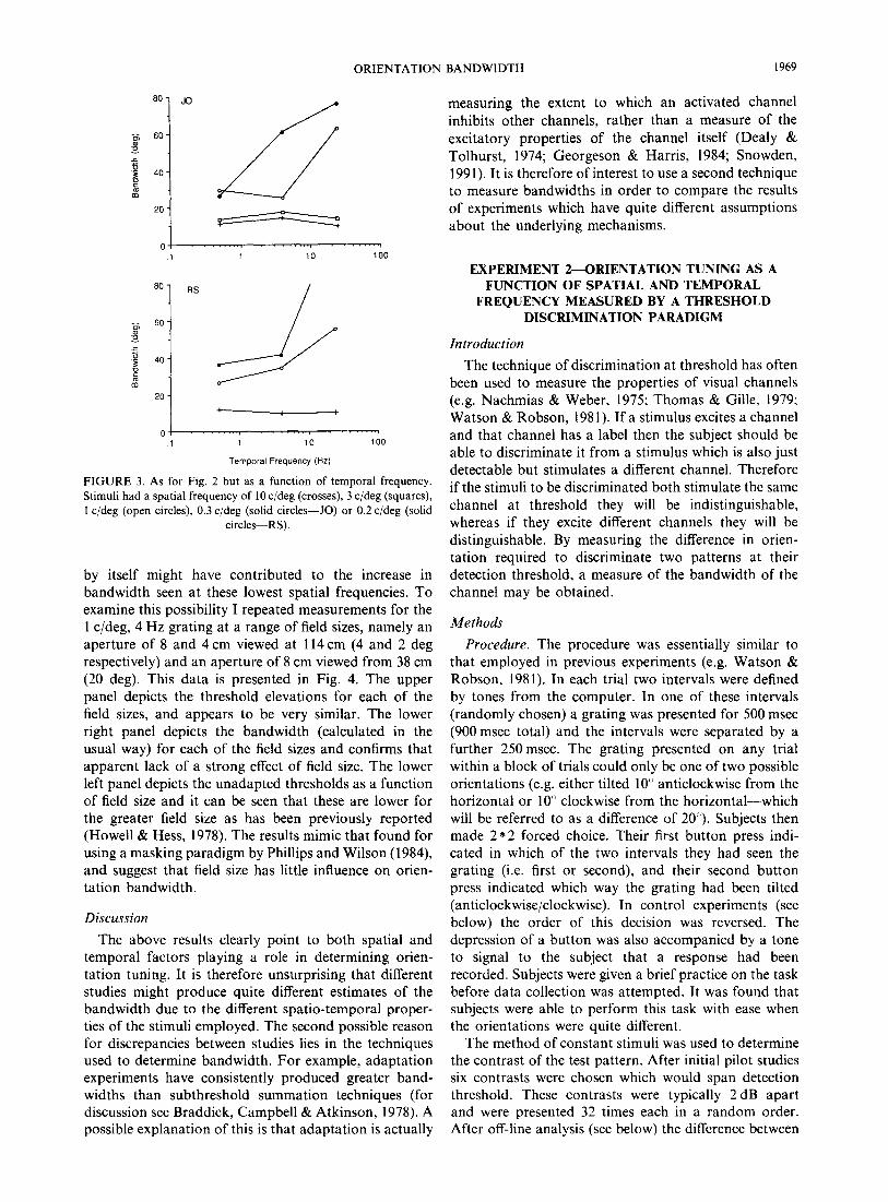
by itself might have contributed to the increase in bandwidth seen at these lowest spatial frequencies. To examine this possibility I repeated measurements for the 1 c/deg, 4 Hz grating at a range of field sizes, namely an

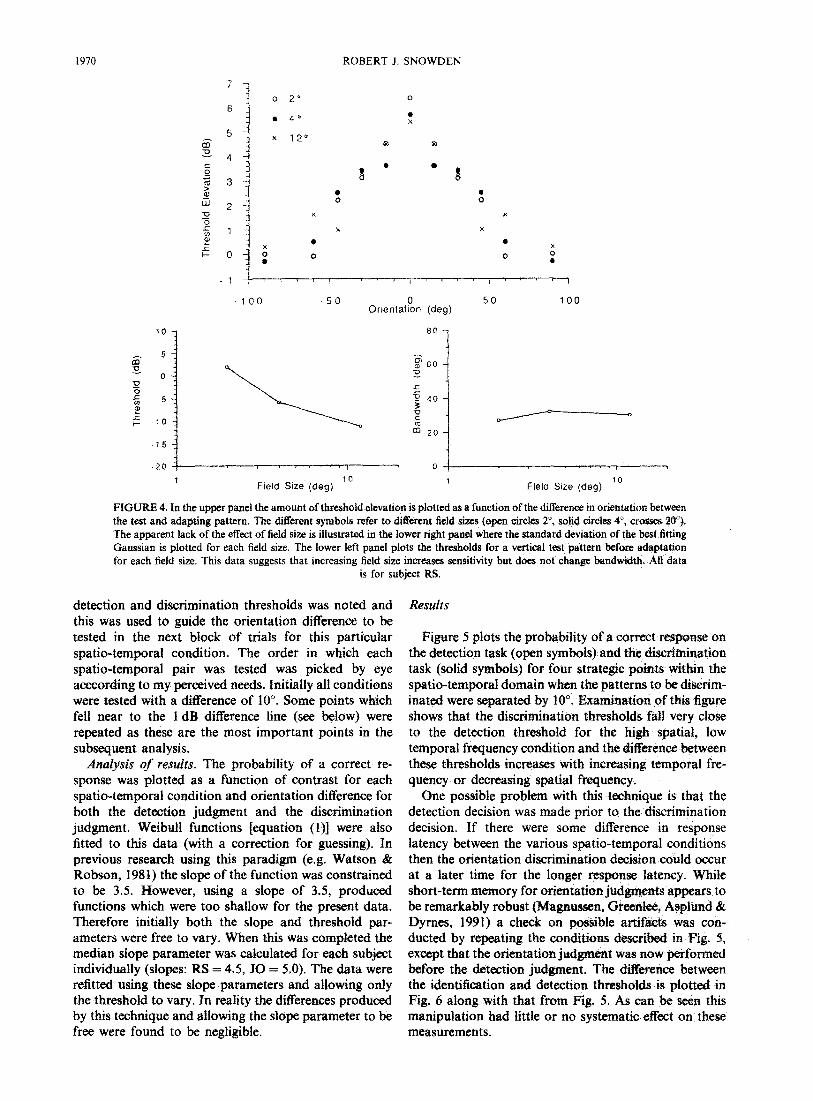
aperture of 8 and 4 cm viewed at 114 cm (4 and 2 deg respectively) and an aperture of 8 cm viewed from 38 cm (20 deg). This data is presented in Fig. 4. The upper panel depicts the threshold elevations for each of the field sizes, and appears to be very similar. The lower right panel depicts the bandwidth (calculated in the usual way) for each of the field sizes and confirms that apparent lack of a strong effect of field size. The lower left pane1 depicts the unadapted thresholds as a function of field size and it can be seen that these are lower for the greater field size as has been previously reported (Howell & Hess, 1978). The results mimic that found for using a masking paradigm by Phillips and Wilson (1984) and suggest that field size has little influence on orientation bandwidth.

Discussion

The above results clearly point to both spatial and temporal factors playing a role in determining orientation tuning. It is therefore unsurprising that different studies might produce quite different estimates of the bandwidth due to the different spatio-temporal properties of the stimuli employed. The second possible reason for discrepancies between studies lies in the techniques used to determine bandwidth. For example, adaptation experiments have consistently produced greater bandwidths than subthreshold summation techniques (for discussion see Braddick, Campbell & Atkinson, 1978). A possible explanation of this is that adaptation is actually

measuring the extent to which an activated channel

inhibits other channels, rather than a measure of the

excitatory properties of the channel itself (Dealy &

Tolhurst, 1974; Georgeson & Harris, 1984; Snowden, 199 1). It is therefore of interest to use a second technique to measure bandwidths in order to compare the results of experiments which have quite different assumptions about the underlying mechanisms.

EXPERIMENT 2-ORIENTATION TUNING AS A FUNCTION OF SPATIAL AND TEMPORAL

FREQUENCY MEASURED BY A THRESHOLD DISCRIMINATION PARADIGM

Introduction

The technique of discrimination at threshold has often been used to measure the properties of visual channels (e.g. Nachmias & Weber, 1975; Thomas & Gille, 1979; Watson & Robson, 198 1). If a stimulus excites a channel and that channel has a label then the subject should be able to discriminate it from a stimulus which is also just detectable but stimulates a different channel. Therefore if the stimuli to be discriminated both stimulate the same

channel at threshold they will be indistinguishable, whereas if they excite different channels they will be distinguishable. By measuring the difference in orientation required to discriminate two patterns at their detection threshold, a measure of the bandwidth of the channel may be obtained.

Methods

Procedure. The procedure was essentially similar to that employed in previous experiments (e.g. Watson & Robson, 1981). In each trial two intervals were defined by tones from the computer. In one of these intervals

(randomly chosen) a grating was presented for 500 msec (900 msec total) and the intervals were separated by a further 250 msec. The grating presented on any trial within a block of trials could only be one of two possible orientations (e.g. either tilted 10” anticlockwise from the horizontal or 10” clockwise from the horizontal-which will be referred to as a difference of 20”). Subjects then made 2*2 forced choice. Their first button press indicated in which of the two intervals they had seen the grating (i.e. first or second), and their second button press indicated which way the grating had been tilted (anticlockwise/clockwise). In control experiments (see below) the order of this decision was reversed. The depression of a button was also accompanied by a tone to signal to the subject that a response had been recorded. Subjects were given a brief practice on the task before data collection was attempted. It was found that subjects were able to perform this task with ease when the orientations were quite different.

The method of constant stimuli was used to determine the contrast of the test pattern. After initial pilot studies six contrasts were chosen which would span detection threshold. These contrasts were typically 2 dB apart and were presented 32 times each in a random order. After off-line analysis (see below) the difference between


-50 Onentatk~ (deg)

50 100

1 Field Size (deg)

10 1 Field Size (deg) lo

FIGURE 4. In the upper panel the amount of threshoId elevation is plotted as a function of the difference in orientation between the test and adapting pattern. The different sytubofs refer to different gefd sizes (open circles 2”, s&d circles 4”, erossea 20”). The apparent lack of the effect of field size is illustrated in the lower right panel where the standard deviation of the best fitting Gaussian is plotted for each field size. The lower left panel plots the thresholds for a vertical test pattern before adaptation for each field size. This data suggests that increasing field size increases sensitivity but does not change bandwidth. All data

is for subject RS.

detection and discrimination thresholds was noted and this was used to guide the orientation difference to be tested in the next block of trials for this particular spatio-temporal condition. The order in which each spatio-temporal pair was tested was picked by eye acccording to my perceived needs. Initially all conditions were tested with a difference of 10”. Some points which fell near to the 1 dB difference line (see below) were repeated as these are the most important points in the subsequent analysis.

Analysis of results. The probability of a correct response was plotted as a function of contrast for each spatio-temporal condition and orientation difference for both the detection judgment and the discrimination judgment. Weibull functions [equation (t)] were also fitted to this data (with a correction for guessing). In previous research using this paradigm (e.g. Watson & Robson, 1981) the slope of the function was constrained to be 3.5. However, using a slope of 3.5, produced functions which were too shallow for the present data. Therefore initially both the slope and threshold parameters were free to vary. When this was completed the median slope parameter was calculated for each subject individually (slopes: RS = 4.5, JO = 5.0). The data were refitted using these slope parameters and allowing only the threshold to vary. In reality the differences produced by this technique and allowing the slope parameter to be free were found to be negligible.

Results

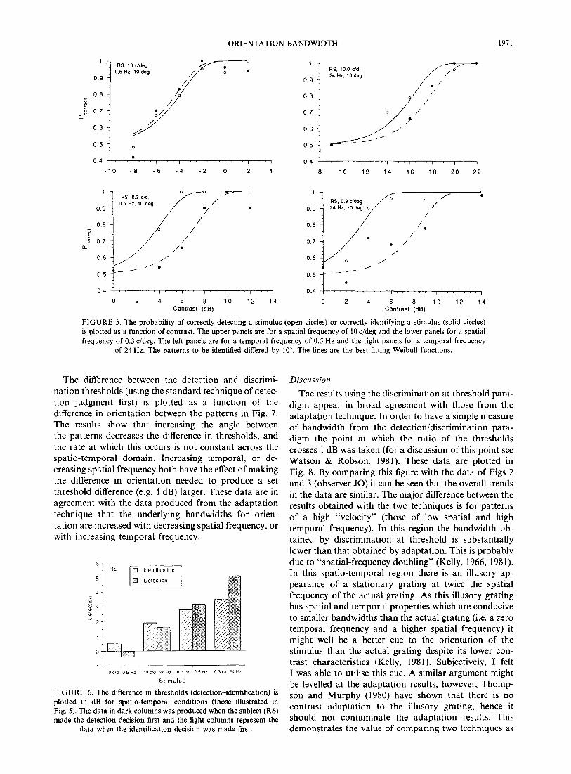
Figure 5 plots the probability of a currect response on the detection task (open symbols) and the &s&nination task (solid symbols) for four straEegic points within the spatio-temporal domain when the patterns to be discriminated were separated by 10”. Examination of this figure shows that the discrimination thresholds fall very close to the detection threshold for the high spatial, low temporal frequency condition and the difference between these thresholds increases with increasing temporal frequency or decreasing spatial frequency.

One possible problem with this technique is that the detection decision was made prior to the dissemination decision. If there were some difference in response latency between the various spatio-temporal conditions then the orientation discrimination decision could occur at a later time for the longer response latency. While short-term memory for orientation judgments appears to be remarkably robust (Magnussen, Greenlee, Asplund & Dyrnes, 1991) a check on possible artifacts was con- ducted by repeating the conditions described in Fig. 5, except that the orientation judgment was now performed before the detection judgment. The difference between the identification and detection thresholds is plotted in Fig. 6 along with that from Fig. 5. As can be seen this manipulation had little or no systematic effect on these measurements,


1

0.9

0.8 5 E 5 0.7

a

0.6

0.5

0.4

: RS. 10 cJdeg

: 0.5 Hz. 10 deg

l- : RS. 10.0 c/d,

0.9 24 Hz. 10deg y

0.8 7

0.7 y

0.6 :

0.5 -

0.4 1, 1 I, 1, IS 1, ,I * 1 / - 1 r I,, I,, 1, 8 10 12 14 16 16 20 22

0.4/ 0.4 ~,.,:.,,,..,,,,.,,..,,..,,..,

0 2 4 6 8 10 12 14 0 2 4 6 8 10 12 14 Contrast (dB) Contrast (d(3)

FIGURE 5. The probability of correctly detecting a stimulus (open circles) or correctly identifying a stimulus (solid circles)

is plotted as a function of contrast. The upper panels are for a spatial frequency of 10 c/deg and the lower panels for a spatial

frequency of 0.3 c/deg. The left panels are for a temporal frequency of 0.5 Hz and the right panels for a temporal frequency

of 24 Hz. The patterns to be identified differed by 10”. The lines are the best fitting Weibull functions.

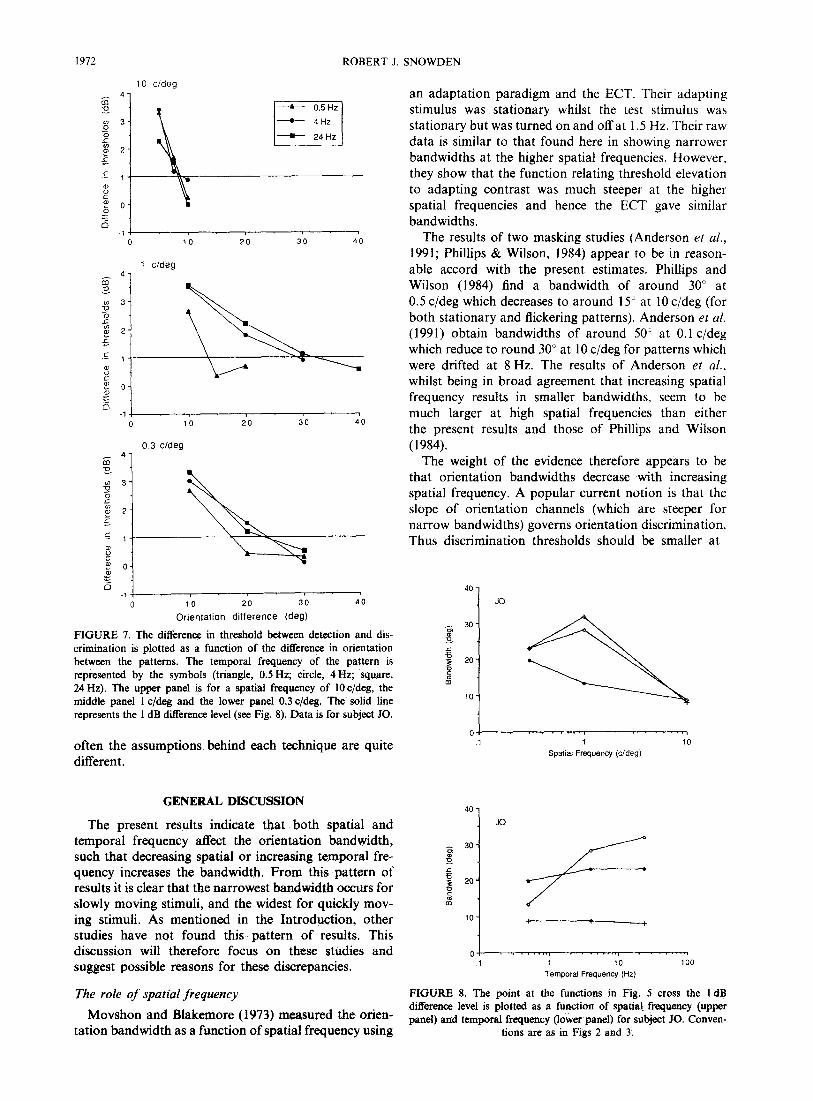
The difference between the detection and discrimination thresholds (using the standard technique of detection judgment first) is plotted as a function of the difference in orientation between the patterns in Fig. 7. The results show that increasing the angle between the patterns decreases the difference in thresholds, and the rate at which this occurs is not constant across the spatio-temporal domain. Increasing temporal, or decreasing spatial frequency both have the effect of making the difference in orientation needed to produce a set threshold difference (e.g. 1 dB) larger. These data are in agreement with the data produced from the adaptation technique that the underlying bandwidths for orientation are increased with decreasing spatial frequency, or with increasing temporal frequency.

5

4 6

23 5 0

2

1

0

FIGURE 6. The difference in thresholds (detection-identification) is

plotted in dB for spatio-temporal conditions (those illustrated in

Fig. 5). The data in dark columns was produced when the subject (RS)

made the detection decision first and the light columns represent the

data when the identification decision was made first.

Discussion

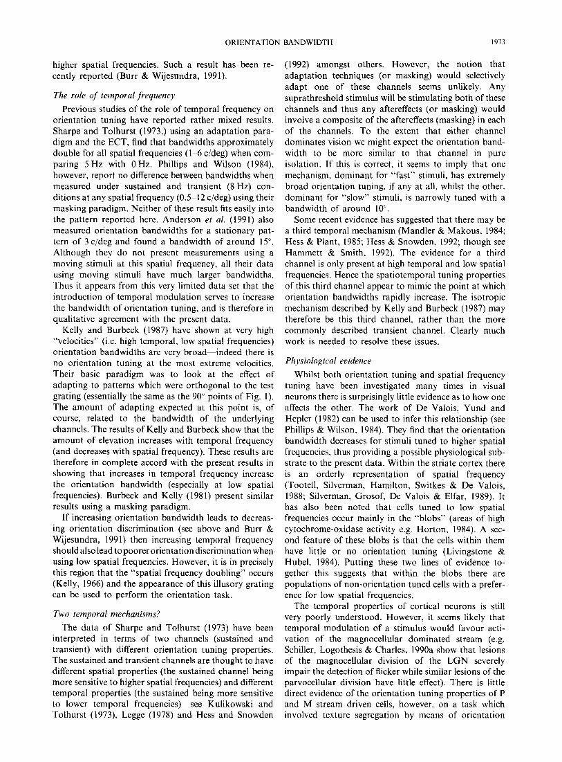
The results using the discrimination at threshold paradigm appear in broad agreement with those from the adaptation technique. In order to have a simple measure of bandwidth from the detection/discrimination paradigm the point at which the ratio of the thresholds crosses 1 dB was taken (for a discussion of this point see Watson & Robson, 1981). These data are plotted in Fig. 8. By comparing this figure with the data of Figs 2 and 3 (observer JO) it can be seen that the overall trends in the data are similar. The major difference between the results obtained with the two techniques is for patterns of a high “velocity” (those of low spatial and high temporal frequency). In this region the bandwidth obtained by discrimination at threshold is substantially lower than that obtained by adaptation. This is probably due to “spatial-frequency doubling” (Kelly, 1966, 1981). In this spatio-temporal region there is an illusory appearance of a stationary grating at twice the spatial frequency of the actual grating. As this illusory grating has spatial and temporal properties which are conducive to smaller bandwidths than the actual grating (i.e. a zero temporal frequency and a higher spatial frequency) it might well be a better cue to the orientation of the stimulus than the actual grating despite its lower contrast characteristics (Kelly, 198 1). Subjectively, I felt I was able to utilise this cue. A similar argument might be levelled at the adaptation results, however, Thomp- son and Murphy (1980) have shown that there is no contrast adaptation to the illusory grating, hence it should not contaminate the adaptation results. This demonstrates the value of comparing two techniques as

ROBERT J SNOWDEN 1972

10 cideg

iii 4-

- 4th

u -1 I

0 10 20 30 40

1 cfdeg

L! -1 1

0 10 20 30 40

0 3 c/dea

_ -1 -I

0 10 20 30 40

Orientation difference (de@

FIGURE 7. The difference in threshold between detection and discrimination is plotted as a function of the ditference in orientation between the patterns. The temporal frequency of the pattern is represented by the symbols (triangle, 0.5 Hz; circle, 4 Hz; square, 24 Hz). The upper panel is for a spatial frequency of 10 c/deg, the middle panel 1 c/deg and the lower panel 0.3 c/deg. The solid line represents the 1 dB difference level (see Fig. 8). Data is for subject JO.

often the assumptions behind each technique are quite different.

GENERAL DISCUSSION

The present results indicate that both spatial and temporal frequency affect the orientation bandwidth, such that decreasing spatial or increasing temporal frequency increases the bandwidth. From this pattern of results it is clear that the narrowest bandwidth occurs for slowly moving stimuli, and the widest for quickly moving stimuli. As mentioned in the Introduction, other studies have not found this pattern of results. This discussion will therefore focus on these studies and suggest possible reasons for these discrepancies.

The role of spatial frequency

Movshon and Blakemore (1973) measured the orientation bandwidth as a function of spatial frequency using

an adaptation paradigm and the ECT. Their adapting stimulus was stationary whilst the test stimulus was stationary but was turned on and off at I .5 Hz. Their raw data is similar to that found here in showing narrower bandwidths at the higher spatial frequencies. However, they show that the function relating threshold elevation to adapting contrast was much steeper at the higher spatial frequencies and hence the ECT gave similar bandwidths.

The results of two masking studies (Anderson et al.,

1991; Phillips & Wilson, 1984) appear to be in reason- able accord with the present estimates. Phillips and Wilson (1984) find a bandwidth of around 30” at 0.5 c/deg which decreases to around 15” at 10 c/deg (for both stationary and flickering patterns). Anderson et al.

(1991) obtain bandwidths of around 50” at 0.1 c/deg which reduce to round 30” at 10 c/deg for patterns which were drifted at 8 Hz. The results of Anderson et al., whilst being in broad agreement that increasing spatial frequency results in smaller bandwidths, seem to be much larger at high spatial frequencies than either the present results and those of Phillips and Wilson (1984).

The weight of the evidence therefore appears to be that orientation bandwidths decrease with increasing spatial frequency. A popular current notion is that the slope of orientation channels (which are steeper for narrow bandwidths) governs orientation discrimination. Thus discrimination thresholds should be smaller at

40

JO

1

40 -

x) .

G 30- m 9

5 0 2 20

s m

lo-

1

Spatial Frequency (c/deg)

10

F “‘1

1 10 100

Temporal Frequency (Hz)

FIGURE 8. The point at the functions in Fig. 5 cross the 1 dB difference level is plotted as a function of spatial frequency (upper panel) and temporal frequency (lower panel) for subject JO. Conven-

tions are as in Figs 2 and 3.


higher spatial frequencies. Such a result has been re-

cently reported (Burr & Wijesundra, 1991).

The role of temporal frequency

Previous studies of the role of temporal frequency on orientation tuning have reported rather mixed results. Sharpe and Tolhurst (1973,) using an adaptation paradigm and the ECT, find that bandwidths approximately double for all spatial frequencies (l-6 c/deg) when comparing 5 Hz with 0 Hz. Phillips and Wilson (1984) however, report no difference between bandwidths when measured under sustained and transient (8 Hz) con-

ditions at any spatial frequency (0.5-12 c/deg) using their masking paradigm. Neither of these result fits easily into

the pattern reported here. Anderson et al. (1991) also measured orientation bandwidths for a stationary pattern of 3 c/deg and found a bandwidth of around 15”. Although they do not present measurements using a moving stimuli at this spatial frequency, all their data using moving stimuli have much larger bandwidths. Thus it appears from this very limited data set that the introduction of temporal modulation serves to increase the bandwidth of orientation tuning, and is therefore in qualitative agreement with the present data.

Kelly and Burbeck (1987) have shown at very high “velocities” (i.e. high temporal, low spatial frequencies) orientation bandwidths are very broad-indeed there is no orientation tuning at the most extreme velocities. Their basic paradigm was to look at the effect of adapting to patterns which were orthogonal to the test grating (essentially the same as the 90” points of Fig. 1). The amount of adapting expected at this point is, of course, related to the bandwidth of the underlying

channels. The results of Kelly and Burbeck show that the amount of elevation increases with temporal frequency (and decreases with spatial frequency). These results are therefore in complete accord with the present results in showing that increases in temporal frequency increase the orientation bandwidth (especially at low spatial frequencies). Burbeck and Kelly (1981) present similar results using a masking paradigm.

If increasing orientation bandwidth leads to decreasing orientation discrimination (see above and Burr & Wijesundra, 199 1) then increasing temporal frequency should also lead to poorer orientation discrimination when. using low spatial frequencies. However, it is in precisely this region that the “spatial frequency doubling” occurs (Kelly, 1966) and the appearance of this illusory grating can be used to perform the orientation task.

Two temporal mechanisms?

The data of Sharpe and Tolhurst (1973) have been interpreted in terms of two channels (sustained and transient) with different orientation tuning properties. The sustained and transient channels are thought to have different spatial properties (the sustained channel being more sensitive to higher spatial frequencies) and different temporal properties (the sustained being more sensitive to lower temporal frequencies)-see Kulikowski and Tolhurst (1973) Legge (1978) and Hess and Snowden

(1992) amongst others. However, the notion that adaptation techniques (or masking) would selectively

adapt one of these channels seems unlikely. Any suprathreshold stimulus will be stimulating both of these channels and thus any aftereffects (or masking) would involve a composite of the aftereffects (masking) in each of the channels. To the extent that either channel dominates vision we might expect the orientation bandwidth to be more similar to that channel in pure

isolation. If this is correct, it seems to imply that one mechanism, dominant for “fast” stimuli, has extremely broad orientation tuning, if any at all, whilst the other,

dominant for “slow” stimuli, is narrowly tuned with a bandwidth of around 10”.

Some recent evidence has suggested that there may be a third temporal mechanism (Mandler & Makous, 1984;

Hess & Plant, 1985; Hess & Snowden, 1992; though see Hammett & Smith, 1992). The evidence for a third channel is only present at high temporal and low spatial frequencies. Hence the spatiotemporal tuning properties of this third channel appear to mimic the point at which

orientation bandwidths rapidly increase. The isotropic mechanism described by Kelly and Burbeck (1987) may therefore be this third channel, rather than the more commonly described transient channel. Clearly much

work is needed to resolve these issues.

Physiological evidence

Whilst both orientation tuning and spatial frequency tuning have been investigated many times in visual neurons there is surprisingly little evidence as to how one affects the other. The work of De Valois, Yund and Hepler (1982) can be used to infer this relationship (see Phillips & Wilson, 1984). They find that the orientation bandwidth decreases for stimuli tuned to higher spatial frequencies, thus providing a possible physiological sub- strate to the present data. Within the striate cortex there is an orderly representation of spatial frequency (Tootell, Silverman, Hamilton, Switkes & De Valois, 1988; Silverman, Grosof, De Valois & Elfar, 1989). It has also been noted that cells tuned to low spatial frequencies occur mainly in the “blobs” (areas of high cytochrome-oxidase activity e.g. Horton, 1984). A second feature of these blobs is that the cells within them have little or no orientation tuning (Livingstone & Hubel, 1984). Putting these two lines of evidence together this suggests that within the blobs there are populations of non-orientation tuned cells with a preference for low spatial frequencies.

The temporal properties of cortical neurons is still very poorly understood. However, it seems likely that temporal modulation of a stimulus would favour acti- vation of the magnocellular dominated stream (e.g. Schiller, Logothesis & Charles, 1990a show that lesions of the magnocellular division of the LGN severely impair the detection of flicker while similar lesions of the parvocellular division have little effect). There is little direct evidence of the orientation tuning properties of P and M stream driven cells, however, on a task which involved texture segregation by means of orientation


differences Schiller, Logothesis and Charles (1990b) show P lesions to have a large detrimental effect whereas M lesions did not. This suggests that the P stream may carry more information concerning the orientation of the stimulus. Taken together the overall picture is that temporal modulation of a stimulus would favour the M stream which is more poorly tuned for orientation. Thus the present results are consistent with this idea.

REFERENCES

Anderson, S. J., Burr, D. C. & Morrone, M. C. (1991). Two- dimensional spatial and spatial-frequency selectivity of motion- sensitive mechanisms in human vision. Journal ofthe Optical Society of America, A, 8, 134Cb1351.

Blakemore, C. & Campbell, F. W. (1969). On the existence of neurones in the human visual system selectively sensitive to the orientation and size of retinal images. Journal of Physiology, London, 203, 237-260.

Blakemore, C. & Nachmias, J. (1971). The orientation specificity of two visual aftereffects. Journal of Physiology, London, 213, 157-174.

Braddick, O., Campbell, F. W. & Atkinson, J. (1978). Channels in vision: Basic aspects. In Held, R., Leibowitz, H. W. & Teuber, H. L. (Ed.), Handbook of sensory physiology. Berlin: Springer.

Burbeck, C. A. &Kelly, D. H. (1981). Contrast gain measurements and the transient/sustained dichotomy. Journal of the Optical Society of America, 71, 1335-1342.

Burr, D. C. & Wijesundra, S.-A. (1991). Orientation discrimination depends on spatial frequency. Vision Research, 31, 1449-1452.

Campbell, F. W. & Kulikowski, J. J. (1966). Orientation selectivity of the human visual system. Journal of Physiology, London, 187,437-445.

Dannemiller, J. L. & Ver Hoeve, J. N. (1990). Two-dimensional approach to psychophysical orientation tuning. Journal of the Optical Society of America, A, 7, 141-151.

Dealy, R. S. & Tolhurst, D.. J. (1974). Is spatial adaptation an after-effect of prolonged inhibition? Journal of Physiology, London, 241, 261-270.

De Valois, R. L., Yund, E. W. & Hepler, N. K. (1982). The orientation and direction selectivity of cells in macaque visual cortex. Vision

Research, 22, 531-544. Georgeson, M. A. (1985). The effect of spatial adaptation on perceived

contrast. Spatial Vision, I, 1033112. Georgeson, M. A. & Harris, M. J. (1984). Spatial selectivity ofcontrast

adaptation: Models and data. Vision Research, 24, 729-741. Graham, N. V. S. (1989). Visual pattern analysers. Oxford: Oxford

University Press. Hammett, S. T. & Smith, A. (1992). Two temporal channels or three?

A re-evaluation. Vision Research, 32, 285-291. Hess, R. F. & Plant, G. T. (1985). Temporal frequency discrimination

in human vision: Evidence for an additional mechanism in the low spatial and high temporal frequency region. Vision Research, 25, 1493-1500.

Hess, R. F. & Snowden, R. J. (1992). Temporal properties of human visual filters: Number, shapes and spatial covariation. Vision Re- search, 32, 47-59.

Horton, J. C. (1984). Cytochrome oxidase patches: A new cytoarchi- tectonic feature of monkey cortex. PhiIosophical Transactions of the Royal Society of London (Biology), 304, 199-253.

Howell, E. R. & Hess, R. F. (1978). The functional area to summation to threshold for sinusoidal gratings. Vision Research, 18, 369-374.

HubeL D. & Weisel, T. (1962). Receptive fields, binocular interaction and functional architecture in the cat’s visual cortex. Journal of Physiology, London, f60, 106154.

Hubel, D. & Weisel, T. (1968). Receptive fields and functional architecture of the monkey striate cortex. Journal of Physiology, London, 155, 215-243.

Kelly, D. H. (1966). Frequency doubling in visual responses. Journal of the Optical Society of America, 56, 162881633.

Kelly, D. H. (1981). Nonlinear responses to flickering sinusoidal gratings. Journal of the Optical Society oJ’ Amerrca, 71, 1051 1055.

Kelly, D. H. & Burbeck, C. A. (1987). Further evidence for a broadband isotropic mechanism sensitive to high velocity stimuli. Vision Research, 27, 1527-l 537.

Kulikowski, J. J. & King-Smith, P. E. (1973). Spatial arrangement of line, edge, and grating detectors revealed by subthreshold summation. Vision Research, 13, 145551478.

Kulikowski, J. J. & Tolhurst, D. J. (1973). Psychophysical evidence for sustained and transient detectors in human vision. Journa/ OJ Physiology, London, 232, 149-162.

Legge, G. E. (1978). Sustained and transient mechanisms in human vision: Temporal and spatial properties. Vision Research, 18, 69-8 1.

Livingstone, M. S. & Hubel, D. H. (1984). Anatomy and physiology of a color system in the primate visual cortex. Journal of Neuro- science, 4, 309-356.

Magnussen, S., Greenlee, M. W., Asplund, R. & Dymes, S. (1991). Stimulus-specific mechanisms of visual short-term memory. Vision Research, 31, 1213-1219.

Mandler, M. B. & Makous, W. (1984). A three channel model of temporal frequency perception. Vision Research, 24, 1881-1887.

Movshon, J. A. & Blakemore, C. (1973). Orientation and spatial selectivity in human vision. Perception, 2, 5360.

Nachmias, J. & Weber, A. (1975). Discrimination of simple and complex gratings. Vision Research, 15, 217-233.

Phillips, G. C. & Wilson, H. R. (1984). Orientation bandwidths of spatial mechanisms measured by masking. Journal of the Optical Society of America, A, I. 226232.

Ross, J. & Speed, H. D. (1991). Contrast adaptation and contrast masking in human vision. Proceedings of the Royal Society of London, 246, 61-69.

Schiller, P. H., Logothesis, N. K. & Charles, E. R. (1990a). Role of the color-opponent and broad-band channels in vision. Visual

Neuroscience, 5, 321-346. Schiller, P. H., Logothetis, N. K. & Charles, E. R. (1990b). Functions

of the colour-opponent and broad-band channels of the visual system. Nature, 343, 68870.

Sharpe, C. R. & Tolhurst, D. J. (1973). The effects of temporal modulation on the orientation channels of the human visual system. Perception, 2, 23-29.

Silverman, M. S., Grosof, D. H., De Valois, R. L. & Elfar, S. D. (1989). Spatial-frequency organization in primate striate cortex. Proceedings of the National Academy of Science, U.S.A., 86, 711-715.

Snowden, R. J. (1991). Measurement of visual channels by contrast adaptation. Proceedings of the Royal Society of London B, 246, 53359.

Stromeyer, C. F. III, Klein, S. & Sternheim, C. E. (1977). Is spatial adaptation caused by prolonged inhibition? Vision Research, 17,

603606. Swift, D. J. & Smith, R. A. (1982). An action spectrum for spatial-

frequency adaptation. Vision Research, 22, 235-246. Thomas, J. P. & Gille, J. (1979). Bandwidth of orientation detectors in

human vision. Journal of the Optical Society of America. 69,652-660.

Thompson, P. & Murphy, B. J. (1980). Adaptation to a “spatial- frequency doubled” stimulus. Perception, 9, 523-528.

Tootell, R. B. H., Silverman, M. S., Hamilton, S. L., Switkes, E. & De Valois, R. L. (1988). Functional anatomy of macaque striate cortex. V. Spatial frequency. Journal of‘ Neuroscience, 8, 1610-1624.

Watson, A. B. & Pelli, D. G. (1983). QUEST: A Bayesian adaptive psychometric method. Perception and Psychophysics, 33, 113-120.

Watson, A. B. & Robson, J. G. (1981). Discrimination at threshold: Labelled detectors in human vision. Vision Research, 21, 1115-I 122.

Acknowledgements-My thanks to Andrew Smith for reading an earlier draft of this manuscript, and to Joanne Orchard for technical assistance.

Documents

Orientation Bandwidth: the Effect of Spatial and Temporal ...psych.cf.ac.uk/home2/snowden/1992_VisionRes_Snowden.pdf · no orientation specific adaptation-implying that the ... bandwidth