Embed Size (px)
Citation preview
OSCILLATOR DESIGN USINGMODERN NONLINEAR CAE
TECHNIQUES
Network Measurements Division1400 Fountaingrove Parkway
Santa Rosa, CA 95401-1799
AUTHORS:Michal OdyniecJeff Patterson
Robert D. AlbinAndy Howard
RF & MicrowaveMeasurementSymposiumandExhibition
r/iO- HEWLETT~~ PACKARD
© 1990 Hewlett-Packard Company
www.HPARCHIVE.com
ABSTRACT
An overview of the design of RF and microwave large signal oscillators highlights the use of modern nonlinear CAE tools.
Traditional forms of oscillator analysis using S-parameters are first reviewed. Then the techniques using the new harmonicbalance nonlinear simulator are outlined. An RF VCO and a microwave YIG oscillator are used as case studies. In both casesdesign strategies are presented along with simulated data compared to actual measurements.
The authors thank Ms. Mary Fewel, Mr. Roger Swearingen, and Mr. Jim Fitzpatrick for helpful comments made on themanuscript.
AUTHORS
Michal Odyniec received his MS in Applied Mathematics and PhD in Electrical Engineering, both from the Technical Universityof Warsaw, Poland. From 1981-1984, Michal was a visiting faculty member at the University of California at Berkeley. In 1985 hejoined Microsource, Inc. where he became a project leader responsible for designing wide-band microwave oscillators. In 1989,Michal joined HP's Network Measurements Division in Santa Rosa, California where he works on nonlinear CAE.
Jeff Patterson joined HP in 1981 after receiving his BSEE from Rice University in Houston, Texas. He worked as a productionengineer from 1981-1985 with responsibility for various families of spectrum analyzers. From 1986 to 1988, Jeff was a member ofthe new product introduction team for the portable family of spectrum analyzers. Since then, he has worked in R&D on low noiseoscillator design.
Robert D. (Dale) Albin received his BSEE degree in 1977 from the University of Texas at Arlington, and MSEE degree fromStanford University in 1980. After joining the Microwave Technology Division of HP in 1977, Dale was a Production Engineerworking on GaAs FET testing and processing. He then joined HP's Network Measurements Division where he was a projectleader on millimeter source modules and project manager for lightwave sources and receivers. He is currently working on YIGoscillators.
Andy Howard is an R&D engineer at HP's Network Measurements Division in Santa Rosa, California. Andy earned his BSEE in1983 and MSEE in 1985, both from the University of California in Berkeley. While earning his MS, Andy learned Japanese andspent nine months working at NEC's Central Research Laboratories in Japan where he investigated an analog-to-digitalconversion algorithm. After joining HP in 1985, Andy developed scalar network detectors and a bridge. He is currently workingon YIG oscillator development.
www.HPARCHIVE.com
Oscillator Design Using Modern Nonlinear CAE Techniquesr/"~ HEWLETT 1~~ PACKARD
Slide 1 INTRODUCTION Slide 3 REVIEW OF OSCILLATORS
OSCILLATOR DESIGNUSING
NON-LINEAR CAE
'-- M::;;":.:.,-J
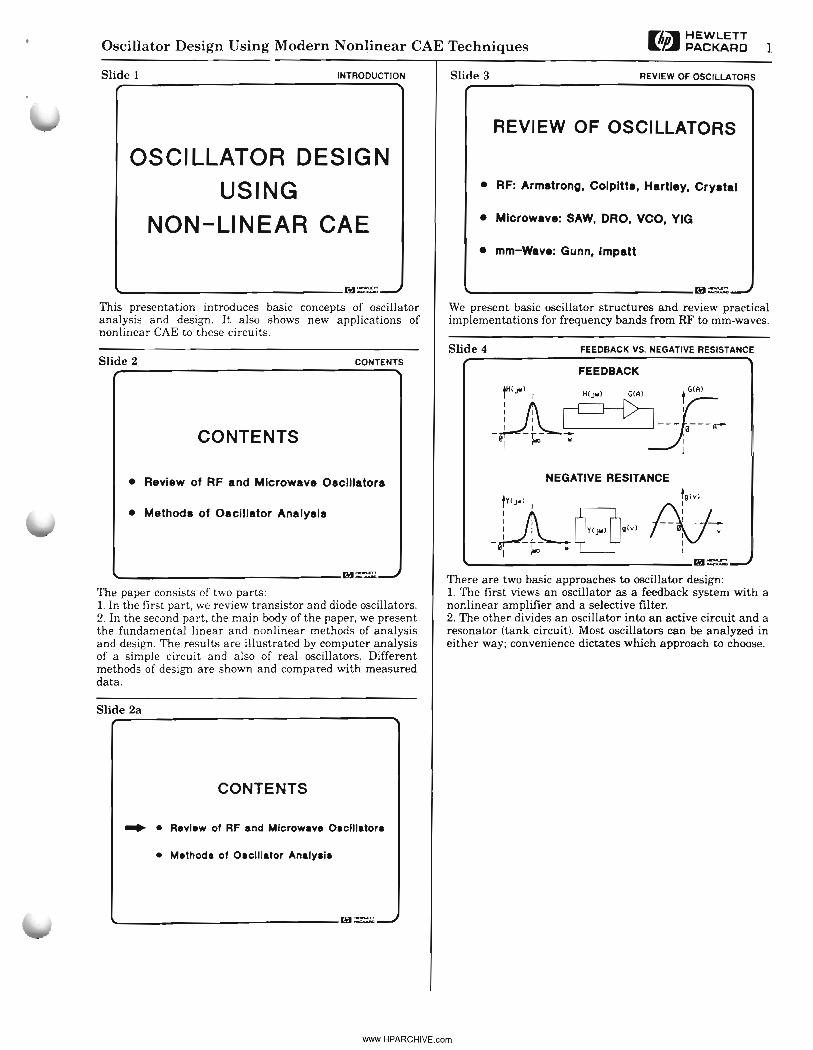
This presentation introduces basic concepts of oscillatoranalysis and design. It also shows new applications ofnonlinear CAE to these circuits.
REVIEW OF OSCILLATORS
• RF: Armatrong, Colpitta. Hartley. Cryatal
• Microwave: SAW, DRO. VCO, YIG
• mm-Wave: Gunn. Impatt
'- M---..;;-J
We present basic oscillator structures and review practicalimplementations for frequency bands from RF to mm-waves.
Slide 2
CONTENTS
CONTENTS
Slide 4 FEEDBACK VS. NEGATIVE RESISTANCE
FEEDBACK
• Review of RF and Microwave OscllIators
• Methods of Oscillator Analysis
'- M---..;;~
The paper consists of two parts:1. In the first part, we review transistor and diode oscillators.2. In the second part, the main body of the paper, we presentthe fundamental linear and nonlinear methods of analysisand design. The results are illustrated by computer analysisof a simple circuit and also of real oscillators. Differentmethods of design are shown and compared with measureddata.
Slide 2a
CONTENTS
.. • Review of RF and Microwave Oaematora
• Methoda of Oaemator AnalyaJa
'-- M::::-:;;~
NEGATIVE RESITANCE
tYCJw) r9 (V)
i 0Q3cJW)gCv) ~__J-;-J.-l}~ I .-W-al I"" W I
'-- M"';';:.,-J
There are two basic approaches to oscillator design:1. The first views an oscillator as a feedback system with anonlinear amplifier and a selective fJ1ter.2. The other divides an oscillator into an active circuit and aresonator (tank circuit). Most oscillators can be analyzed ineither way; convenience dictates which approach to choose.
www.HPARCHIVE.com
2F/i;' HEWLETT~~ PACKARD Oscillator Design Using Modern Nonlinear CAE Techniques '
Slide 5 BASIC FEEDBACK STRUCTURE called "audion" at that time) and are still used [1].
BASIC FEEDBACK CONFIGURATIONSlide 8 CRYSTAL AND SAW OSCILLATORS
CRYSTAL OSCILLATOR SAW OSCILLATOR
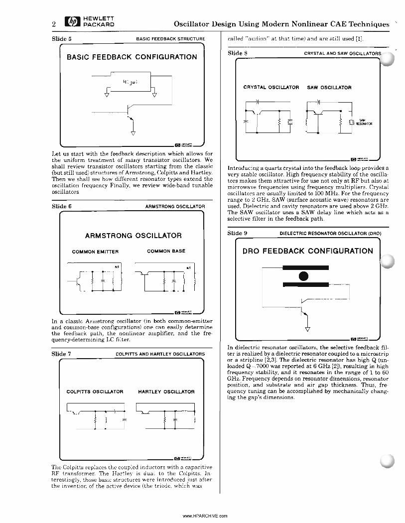
'- m=Let us start with the feedback description which allows forthe uniform treatment of many transistor oscillators. Weshall review transistor oscillators starting from the classic(but still used) structures of Armstrong, Colpitts and Hartley.Then we shall see how different resonator types extend theoscillation frequency Finally, we review wide-band tunableoscillators.
Slide 6 ARMSTRONG OSCILLATOR
'-- m=Introducing a quartz crystal into the feedback loop provides avery stable oscillator. High frequency stability of the oscillators makes them attractive for use not only at RF but also atmicrowave frequencies using frequency multipliers. Crystaloscillators are usually limited to 100 MHz. For the frequencyrange to 2 GHz, SAW (surface acoustic wave) resonators areused. Dielectric and cavity resonators are used above 2 GHz.The SAW oscillator uses a SAW delay line which acts as aselective filter in the feedback path.
ARMSTRONG OSCILLATOR Slide 9 DIELECTRIC RESONATOR OSCILLATOR (ORO)
COMMON EMITTER COMMON BASE ORO FEEDBACK CONFIGURATION
'- m=In a classic Armstrong oscillator (in both common-emitterand common-base configurations) one can easily determinethe feedback path, the nonlinear amplifier, and the frequency-determining LC filter.
•'- m=
COLPITTS OSCILLATOR
Slide 7 COLPITTS AND HARTLEY OSCILLATORS
HARTLEY OSCILLATOR
In dielectric resonator oscillators, the selective feedback filter is realized by a dielectric resonator coupled to a microstripor a stripline [2,3J. The dielectric resonator has high Q (unloaded Q=7000 was reported at 6 GHz [2]), resulting in highfrequency stability, and it resonates in the range of 1 to 60GHz. Frequency depends on resonator dimensions, resonatorposition, and substrate and air gap thickness. Thus, frequency tuning can be accomplished by mechanically changing the gap's dimensions.
'- m=The Colpitts replaces the coupled inductors with a capacitiveRF transformer. The Hartley is dual to the Colpitts. Interestingly, those basic struct~res were introduced just afterthe invention of the active device (the triode, which was
www.HPARCHIVE.com
Oscillator Design Using Modern Nonlinear CAE TechniquesFlio- HEWLETT 3~I:JII PACKARD
Slide 10 TUNABLE OSCILLATORS VCO AND YIG
TUNABLE OSCILLATORS
(lnP) .1 W at 100 GHz with 2% efficiency (InP)
An IMPATI diode (or a diode in IMPATI mode) oscillates to100 GHz, and even to 400 GHz (using higher harmonics).
yeo
The output powers are about: 10 W at 10 GHz with 20%efficiency (GaAs or Si) 1.5 W at 50 GHz with 10% efficiency(GaAs or Si) 60 mW at 100 GHz with 1% efficiency (GaAs) 50mW at 220 GHz with 1% efficiency (Si)
CAVITY DIODE OSCILLATOR
Both Gunn and IMPATI diodes can be viewed as a negativeresistance in parallel with capacitance.o...
YIGSlide 12 CAVITY OSCILLATORS
]
mNEGATIVE RESISTANCE CONFIGURATION
LCCrystalSAWCavity
DRYIG
'- M~
([-I-I Waveguide
'- M~
Cavity
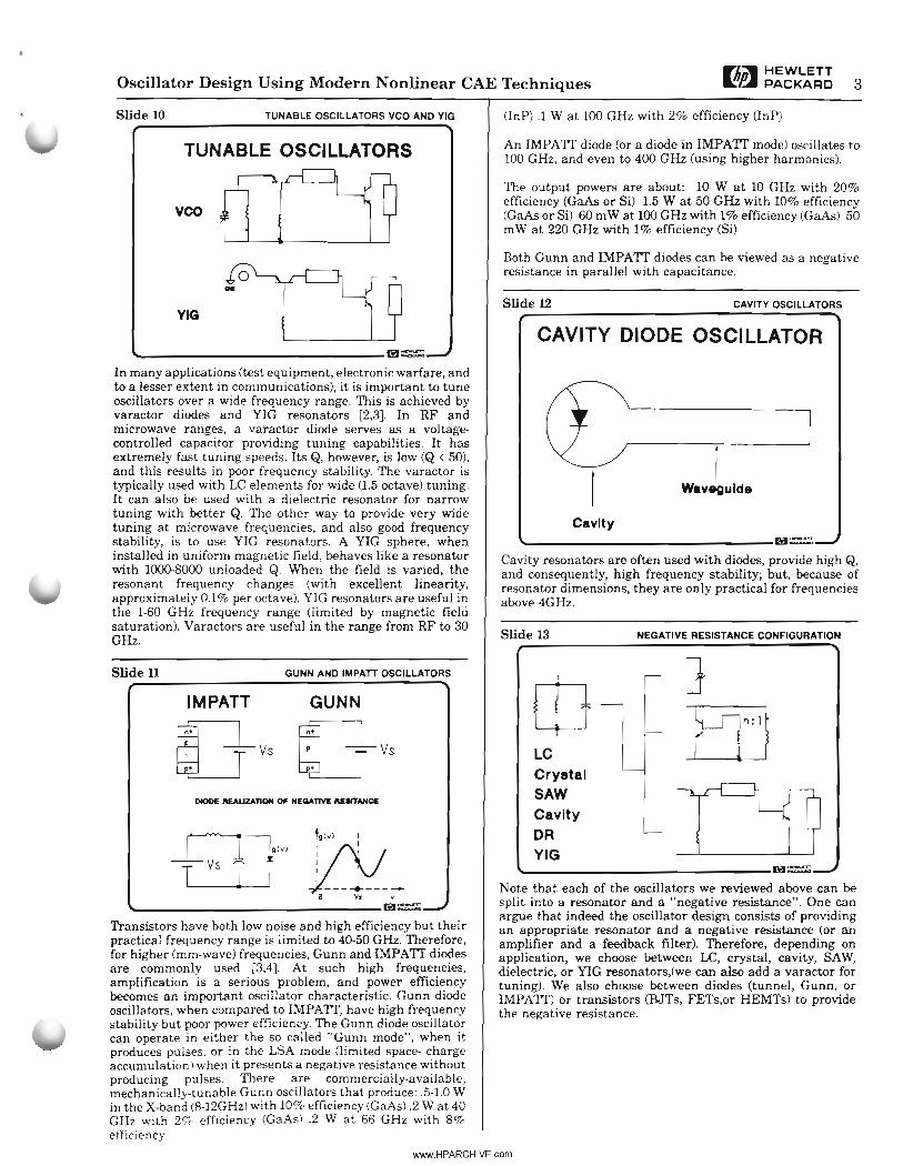
Cavity resonators are often used with diodes, provide high Q,and consequently, high frequency stability; but, because ofresonator dimensions, they are only practical for frequenciesabove 4GHz.
Slide 13
Note that each of the oscillators we reviewed above can besplit into a resonator and a "negative resistance". One canargue that indeed the oscillator design consists of providingan appropriate resonator and a negative resistance (or anamplifier and a feedback filter). Therefore, depending onapplication, we choose between LC, crystal, cavity, SAW,dielectric, or YIG resonators,(we can also add a varactor fortuning). We also choose between diodes (tunnel, Gunn, orIMPATI) or transistors (BJTs, FETs,or HEMTs) to providethe negative resistance.
GUNN
GUNN AND IMPATT OSCILLATORS
~~vs
IMPATT
ruglV )
LlJ /Vi9IV
) iI II I, -+ _e VI II'- M~
Slide 11
'- M~
In many applications (test equipment, electronic warfare, andto a lesser extent in communications), it is important to tuneoscillators over a wide frequency range. This is achieved byvaractor diodes and YIG resonators [2,3]. In RF andmicrowave ranges, a varactor diode serves as a voltagecontrolled capacitor providing tuning capabilities. It hasextremely fast tuning speeds. Its Q, however, is low (Q <50),and this results in poor frequency stability. The varactor istypically used with LC elements for wide (1.5 octave) tuning.It can also be used with a dielectric resonator for narrowtuning with better Q. The other way to provide very widetuning at microwave frequencies, and also good frequencystability, is to use YIG resonators. A YIG sphere, wheninstalled in uniform magnetic field, behaves like a resonatorwith 1000-8000 unloaded Q. When the field is varied, theresonant frequency changes (with excellent linearity,approximately 0.1% per octave). YIG resonators are useful inthe 1-60 GHz frequency range (limited by magnetic fieldsaturation). Varaetors are useful in the range from RF to 30GHz.
Transistors have both low noise and high efficiency but theirpractical frequency range is limited to 40-50 GHz. Therefore,for higher (mm-wave) frequencies, Gunn and IMPATI diodesare commonly used [3,4]. At such high frequencies,amplification is a serious problem, and power efficiencybecomes an important oscillator characteristic. Gunn diodeoscillators, when compared to IMPATI, have high frequencystability but poor power efficiency. The Gunn diode oscillatorcan operate in either the so called "Gunn mode", when itproduces pulses, or in the LSA mode (limited space- chargeaccumulation) when it presents a negative resistance withoutproducing pulses. There are commercially-available,mechanically-tunable Gunn oscillators that produce: .5-1.0 Win the X-band (8-12GHz) with 10% efficiency (GaAs) .2 W at 40GHz with 2% efficiency (GaAsl .2 W at 66 GHz with 8%efficiency
www.HPARCHIVE.com
4Fh;."W HEWLETT~~ PACKARD Oscillator Design Using Modern Nonlinear CAE TechniquL
Slide 14 Slide 16 NONLINEAR METHODS· REVIEW
CONTENTS
• RevIew of RF and MIcrowave Oecillatora
... • Methode of Oecillator Analye'e
________________M~
NON-LINEAR METHODS
• Direct Time-Domain Simulation
• Approximate Methoda
• ·Umltect· Signaia
• Periodic Signaia________________M~
METHODS OF OSCILLATOR ANALYSIS
Slide 15 NONLINEAR METHODS OF OSCILLATORDESIGN
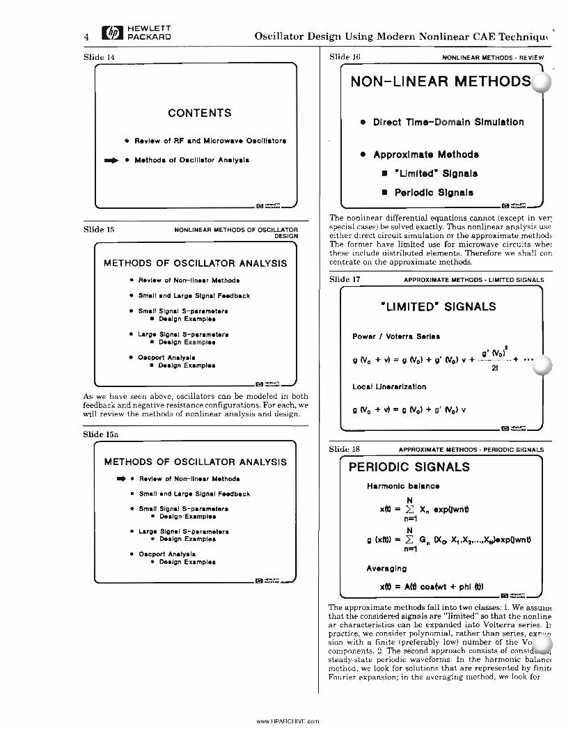
The nonlinear differential equations cannot (except in ver:special cases) be solved exactly. Thus nonlinear analysis use.either direct circuit simulation or the approximate methodEThe former have limited use for microwave circuits wheJthese include distributed elements. Therefore we shall concentrate on the approximate methods.
e Review of Non-linear Methoda
e Small and Large Signa' Feedback
e Small Signal S-parametara• Dealgn examplea
Slide 17 APPROXIMATE METHODS· LIMITED SIGNALS
-LIMITED- SIGNALS
e Large Signal S-parametera• Dealgn Examplea
e Oacport Analyala• Dealgn Examplea
'- M~
As we have seen above, oscillators can be modeled in bothfeedback and negative resistance configurations. For each, wewill review the methods of nonlinear analysis and design.
Slide 15a
Power I Voterra Serl.aI
g' (Vo)g (VO + vl =g (Vo) + g' (Vo) v + + ...
21
Local Unerarlzatlon
g (Vo + vl =g (Vo) + g' (Vo) v
______________M~
Slide 18 APPROXIMATE METHODS· PERIODIC SIGNALS
METHODS OF OSCILLATOR ANALYSIS
.. • Review of Non-linear Methoda
• Small and Large Signal Feedback
• Small Signal S-parametera• Dealgn Examplea
• Large Signal S-parametera• Dealgn examplea
e Oacport Analyala• Dealgn Examplea
'- M~
www.HPARCHIVE.com
PERIODIC SIGNALSHarmonic balance
Nxft) = L: XII .xpOwn~
n=1N
g (xft) = L: Gil (Xo X1,XI,···,x..>expOwn~n=1
Averaging
x(l) =Aft) coa<wt + phI (I)'- M=The approximate methods fall into two classes: 1. We assum(that the considered signals are "limited" so that the nonlinear characteristics can be expanded into Volterra series. Irpractice, we consider polynomial, rather than series, ex"'>sion with a finite (preferably low) number of the Vocomponents. 2. The second approach consists of considsteady-state periodic waveforms. In the harmonic balanctmethod, we look for solutions that are represented by fin it!Fourier expansion; in the averaging method, we look for
Oscillator Design Using Modern Nonlinear CAE TechniquesFlihl HEWLETT~~ PACKARD 5
Signal
• R.vI.w of Non-lIn.ar M.thod.
'- 1¥J~
FEEDBACK DESCRIPTION
v(t) • Jh(t-t' )g(v(t' lldt'
FEEDBACK OSCILLATOR
H(Jw) g(v)
~
tH(JIlI) I
;A-~~~01 ,1lIO III
tg(Vo+vl
T~
Slide 20
'- 1¥J=
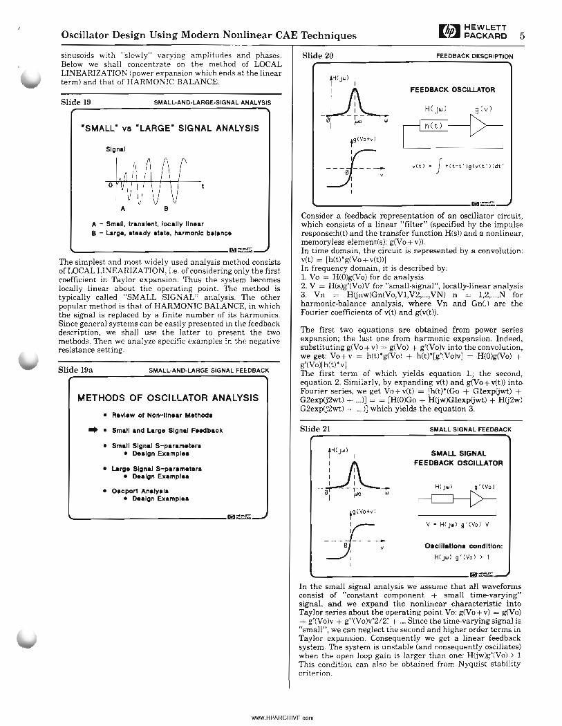
Consider a feedback representation of an oscillator circuit,which consists of a linear "filter" (specified by the impulseresponse:h(t) and the transfer function H(s» and a nonlinear,memoryless element(s): g(Vo+v».In time domain, the circuit is represented by a convolution:v(t) = [h(t)"g(Vo+v(t»]In frequency domain, it is described by:1. Vo = H(O)g(Vo) for dc analysis2. V = H(s)g'(Vo)V for "small-signal", locally-linear analysis3. Vn = H(jnw)Gn(Vo,Vl.V2•...,VN) n = 1,2•... ,N forharmonic-balance analysis, where Vn and GnO are theFourier coefficients of v(t) and g(v(t».
The first two equations are obtained from power seriesexpansion; the last one from harmonic expansion. Indeed,substituting g(Vo+ v) = g(Vo) + g'(Vo)v into the convolution,we get: Vo+v = h(t)"g(Vo) + h(t)"[g'(Vo)v] = H(O)g(Vo) +g'(Vo)[h(t)"v]The first term of which yields equation I.; the second.equation 2. Similarly, by expanding v(t) and g(Vo+v(t) intoFourier series. we get Vo+v(t) = (h(t)"(Go + Glexp(jwt) +G2exp(j2wt) + )] = = [H(O)Go + H(jw)Glexp(jwt) + H(j2w)G2exp(j2wt) + )] which yields the equation 3.
SMALL·AND·LARGE·SIGNAL ANALYSIS
SMALL·AND-LARGE SIGNAL FEEDBACK
sinusoids with "slowly" varying amplitudes and phases.Below we shall concentrate on the method of LOCALLINEARIZATION (power expansion which ends at the linearterm) and that of HARMONIC BALANCE.
o
-SMALL- va -LARGE- SIGNAL ANALYSIS
Slide 19
A - Small, tran.'.nt, locally IIn.arB - Larg., .t••dy .tat., harmonic balance
METHODS OF OSCILLATOR ANALYSIS
Slide 19a
The simplest and most widely used analysis method consistsof LOCAL LINEARIZATION, i.e. of considering only the firstcoefficient in Taylor expansion. Thus the system becomeslocally linear about the operating point. The method istypically called "SMALL SIGNAL" analysis. The otherpopular method is that of HARMONIC BALANCE, in whichthe signal is replaced by a finite number of its harmonics.Since general systems can be easily presented in the feedbackdescription, we shall use the latter to present the twomethods. Then we analyze specific examples in the negativeresistance setting.
• • Small and Larg. Signal FHc:lback Slide 21 SMALL SIGNAL FEEDBACK
• Small Signal S-param.t.r.• De.lgn Exampl••
• Larg. Signal S-param.t.r.• Dealgn Exampl••
• O.cport Analy.l.• De.lgn Exampl••
'- 1¥J= tg(vo+v)
--f--~
SMAll. SIGNALFEEDBACK OSCILLATOR
v • H(JIlI) g'(Vo) V
Oacmatlona condition:
H(JIlI) g'(Vo) ) 1
________________m=In the small signal analysis we assume that all waveformsconsist of "constant component + smaIl time-varying"signal, and we expand the nonlinear characteristic intoTaylor series about the operating point Yo: g(Vo+v) = g(Vo)+ g'(Vo)v + g"(Vo)v'2/2! + ... Since the time-varying signal is"small", we can neglect the second and higher order terms inTaylor expansion. Consequently we get a linear feedbacksystem. The system is unstable (and consequently oscillates)when the open loop gain is larger than one: H(jw)g'(Vo) > 1This condition can also be obtained from Nyquist stabilitycriterion.
www.HPARCHIVE.com
6F/;;' HEWLETT~I:.II PACKARD Oscillator Design Using Modern Nonlinear CAE Techniques
Slide 22 LARGE-SIGNAL FEEDBACK Slide 23a
LARGE SIGNALFEEDBACK OSCILLATOR
~)
Oaclllationa conditionfor v(t) =Acoa (w1):
A = H(Jw) G,(Vo,A)'- M=
METHODS OF OSCILLATOR ANALYSIS
• Review 0' Non-llnear Methocla
• Small and Large Signal Feedback
• • Small Signa' S-parametera• Dealgn Examplea
• Large Signa' S-parametera• Dealgn example.
• Oacport Analy.la• De.lgn Example.
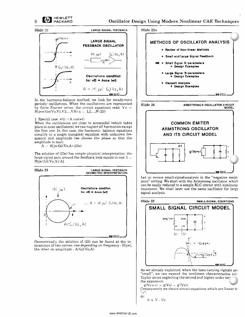
'- M=In the harmonic-balance method, we look for steady-stateperiodic oscillations. When the oscillations are representedby finite Fourier series, the circuit equations read: VnH(jnw)Gn(Vo,Vl,V2,...,VN) n = 1,2,...,N (23)
Slide 24 ARMSTRONG'S OSCILLATOR CIRCUITMODEL
The solution of (23a) has simple physical interpretation: thelarge signal gain around the feedback loop equals to one: 1 =H(jw)[Gl(Vo,A)1A).
1. Special case: vet) - A cos(wt)When the oscillations are close to sinusoidal (which takesplace in most osciJIators), we can neglect all harmonics exceptthe first one. In this case, the harmonic- balance equationssimplify to a single (complex) equation with unknown frequency and amplitude (we choose the phase so that theamplitude is real).
A = H(jw)Gl(Vo,A) (23a) n:1
COMMON EMITERARMSTRONG OSCILLATORAND ITS CIRCUIT MODEL
'- M=LARGE-SIGNAL FEEDBACKGEOMETRIC INTERPRETATION
Slide 23
Oaematlona condlton'or vOl • Acoa lwtl:
'- M=
SMAU-5IGNAL EQUATIONS
= -Gresev
v
---';9-(%+0
SMALL SIGNAL CIRCUIT MODEL
Gdog0CVOlr=Ill :
llclJJI I
Sn ~ !Sr
Slide 25
Let us review small-signal-analysis in the "negative resist·ance" setting. We start with the Armstrong oscillator, whichcan be easily reduced to a simple RLC circuit with nonlinearresistance. We shall later use the same oscillator for largfsignal analysis.
A = H(Jw) G,(Vo,A).1---------i __
t
Geometrically the solution of (23) can be found at the intersection of two curves: one depending on frequency - H(jw),the other on amplitude - A/Gl(Vo,A).
'-- --:. M=As we already explained, when the time-varying signals an"small", we can expand the nonlinear characteristics intcTaylor series neglecting the second and higher order ter-the expansion:
g(Vo+v) = g(Vo) + g'(Vo)vConsequently we obtain circuit equations which are linear iruv":dc:
0= V - Vo
www.HPARCHIVE.com
Oscillator Design Using Modern Nonlinear CAE TechniquesF/,;W HEWLETT 7~t:JII PACKARD
0= 10 - g(Vo) Slide 28 8·20 GHZ OSCILLATOR - DIAGRAMac:
Ldi/dt = - vCdv/dt = i - g'(Vo)v - Gres v
Clearly the circuit oscillates when its total conductance(g'(Vo)+Gres) is negative.
OSCILLATOR MODEL
'- m1=::;:;
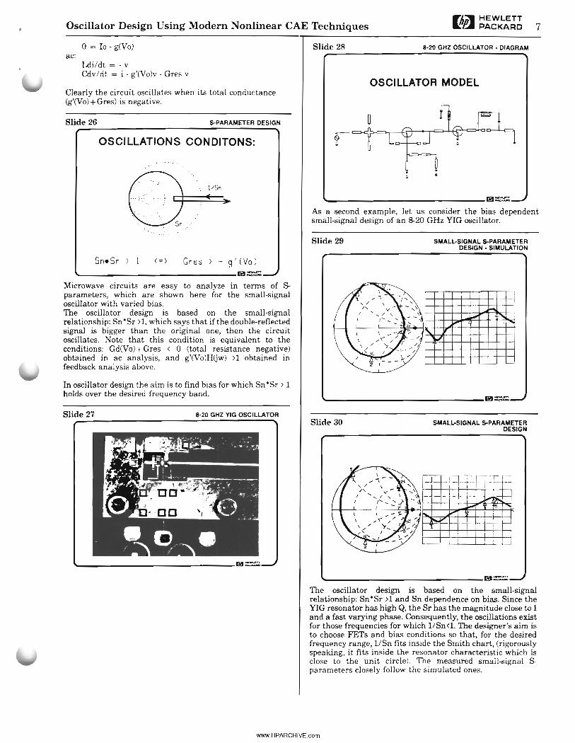
As a second example, let us consider the bias dependentsmall-signal design of an 8-20 GHz YIG oscillator.
l/Sn
S-PARAMETER DESIGN
........
OSCILLATIONS CONDITONS:
Slide 26
Slide 29 SMALL·SIGNAL S-PARAMETERDESIGN· SIMULATION
SneSr ) 1 (=) Gres ) - g'(Vo)_________________m1=::;:;
Microwave circuits are easy to analyze in terms of Sparameters, which are shown here for the small-signaloscillator with varied bias.The oscillator design is based on the small-signalrelationship: Sn ·Sr >1, which says that if the double-reflectedsignal is bigger than the original one, then the circuitoscillates. Note that this condition is equivalent to theconditions: Gd(Vo)+Gres < 0 (total resistance negative)obtained in ac analysis, and g'(Vo)H(jw) >1 obtained infeedback analysis above.
In oscillator design the aim is to find bias for which Sn·Sr >1holds over the desired frequency band. _________________m1=
SMALL·SIGNAL S-PARAMETERDESIGN
Slide 308-20 GHZ YIG OSCILLATOR
'- m1=::;:;
Slide 27
_________________m1=
The oscillator design is based on the small-signalrelationship: Sn·Sr >1 and Sn dependence on bias. Since theYIG resonator has high Q, the Sr has the magnitude close to 1and a fast varying phase. Consequently, the oscillations existfor those frequencies for which lISn <1. The designer's aim isto choose FETs and bias conditions so that, for the desiredfrequency range, 1/Sn fits inside the Smith chart, (rigorouslyspeaking, it fits inside the resonator characteristic which isclose to the unit circle). The measured small-signal g..parameters closely follow the simulated ones.
www.HPARCHIVE.com
8rli~. HEWLETT~~ PACKARD Oscillator Design Using Modern Nonlinear CAE Techniques
Slide 30a Slide 32 LARGE·SIGNAL S-PARAMETERSFOR THE LC OSCILLATOR
METHODS OF OSCILLATOR ANALYSIS
• Review of Non-linear Methoda OSCILLATIONS CONDITIONS rOR vet) • Acos(.,t):
• Small and Large Signal Feec:lback
• Small Signal S-parametera• o.algn Examplea
.. • Large Signal S-parametera• o.algn Examplea
• Oacport Analyala• o.algn examplea
CJ*.., '''.' Sn-Sr: 1
. : J/Sn. '" ..~-
'. Sr·'•• J.. •...•
tI
: C1(Vo,Ag)+ er... Ag- e
B: Ao
--~AI! Gl (Vo,A) -Gre.-A
'- m=
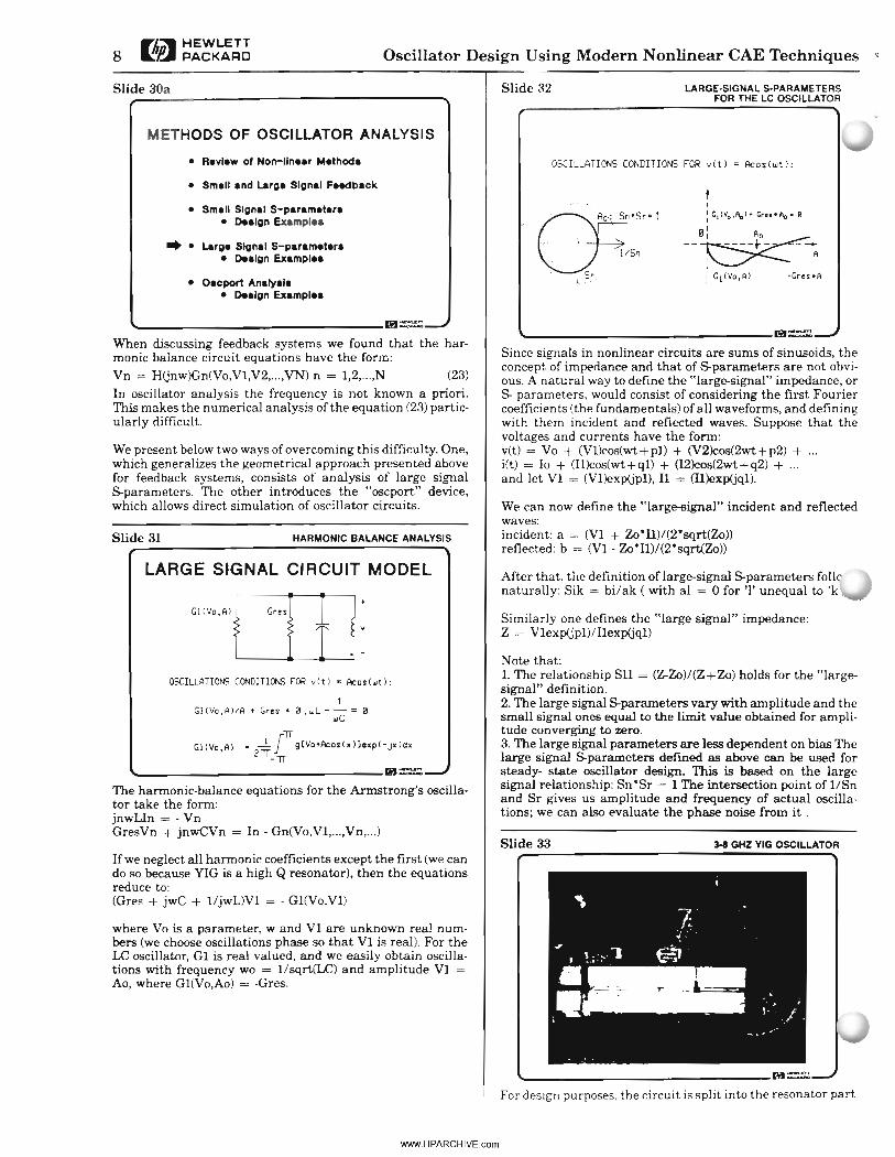
We present below two ways of overcoming this difficulty. One,which generalizes the geometrical approach presented abovefor feedback systems, consists of analysis of large signalS-parameters. The other introduces the "oscport" device,which allows direct simulation of oscillator circuits.
When discussing feedback systems we found that the harmonic balance circuit equations have the form:Vn = H(jnw)Gn(Vo,Vl,V2,... ,VN) n = 1,2,... ,N (23)
In oscillator analysis the frequency is not known a priori.This makes the numerical analysis of the equation (23) particularly difficult.
Slide 31 HARMONIC BALANCE ANALYSIS
'- m=Since signals in nonlinear circuits are sums of sinusoids, theconcept of impedance and that of S-parameters are not obvious. A natural way to define the "large-signal" impedance, orS- parameters, would consist of considering the first Fouriercoefficients (the fundamentals) of all waveforms, and defmingwith them incident and reflected waves. Suppose that thevoltages and currents have the fonn:vet) = Vo + (Vl)cos(wt+pl) + (V2)cos(2wt+p2) + ...i(t) = 10 + (Il)cos(wt+qI) + (I2)cos(2wt+q2) + ...and let VI = (Vl)exp(jpl), Il = (Il)exp(jql).
We can now define the "large-signal" incident and reflectedwaves:incident: a = (VI + Zo·Il)/(2·sqrt(Zo»reflected: b = (VI - Zo·Il)/(2·sqrt(Zo»
LARGE SIGNAL CIRCUIT MODEL
The hannonic-balance equations for the Armstrong's oscillator take the fonn:jnwLln = - VnGresVn + jnwCVn = In - Gn(Vo,Vl,...,Vn,...)
OSCILLATIONS CONDITIa6 rOR vet) • Aco.(.,t):
1Gl(Vo,A)/A + Gre•• ",.,L - - =".,e
GlCVo A) • 2-fir g(Vo+Aco.(x»)exp(-Jxldx, 21r_
1r'- m=
After that, the definition oflarge-signal S-parameters follenaturally: Sik = bi/ak ( with al = 0 for '1' unequal to 'k
3-1 GHZ YIG OSCILLATOR
Similarly one defines the "large signal" impedance:Z = Vlexp(jpl)/Ilexp(jqI)
Note that:1. The relationship S11 = (Z-Zo)/(Z+Zo) holds for the "largesignal" definition.2. The large signal S-parameters vary with amplitude and thesmall signal ones equal to the limit value obtained for amplitude converging to zero.3. The large signal parameters are less dependent on bias Thelarge signal S-parameters defined as above can be used forsteady- state oscillator design. This is based on the largesignal relationship: So·Sr = 1 The intersection point ofl/Snand Sr gives us amplitude and frequency of actual oscillations; we can also evaluate the phase noise from it .
Slide 33
+
"
Gre.
* .
Gl (Vo,A)
Ifwe neglect all hannonic coefficients except the first (we cando so because YIG is a high Q resonator), then the equationsreduce to:(Gres + jwC + l/jwL)Vl = . G1(Vo,vl)
where Vo is a parameter, w and VI are unknown real num·bers (we choose oscillations phase so that VI is real). For theLC oscillator, Gl is real valued, and we easily obtain oscillations with frequency wo = l/sqrt(LC) and amplitude VI =Ao, where Gl(Vo,Ao) = -Gres.
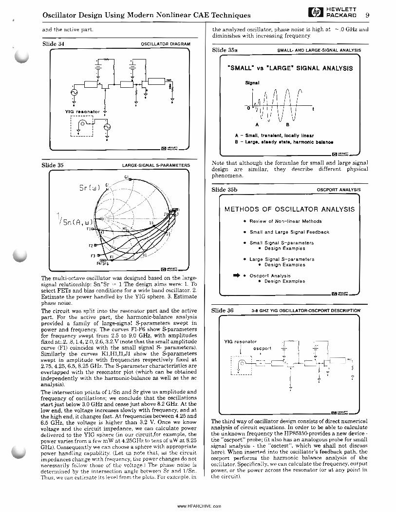
'- m=For design purposes, the circuit is split into the resonator part
www.HPARCHIVE.com
Oscillator Design Using Modern Nonlinear CAE Techniques Fliii'l HEWLETT 9~~ PACKARD
and the active part.
Slide 34 OSCILLATOR DIAGRAM
the analyzed oscillator, phase noise is high at -.0 GHz anddiminishes with increasing frequency.
Slide 35a SMALL- AND LARGE-SIGNAL ANALYSIS
VIG r.aonator--------, .:m:'I ,I II IL__' J .
•_________________lB=
-SMALL- va -LARGE- SIGNAL ANALYSIS
Signal
o
B
A - Small, tranel.nt, locally linearB - Larg., at.ady atat., harmonic balance
_________________lB=
OSCPORT ANALYSIS
3-8 GHZ YIG OSCILLATOR-OSCPORT DESCRIPTION
Slide 35b
VIG resonator --r-lI oscport ~ (________ , I Iin-e-~L..,.....J 1
_________________lH=
_________________lB=
METHODS OF OSCILLATOR ANALYSIS
• Review of Non-linear Methods
• Small and Large Signal Feedback
• Large Signal S-parameters• Design Examples
~ • Oscport Analysis• Design Examples
• Small Signal S-parameters• Design Examples
Note that although the formulae for small and large signaldesign are similar, they describe different physicalphenomena.
Slide 36
The third way of oscillator design consists of direct numericalanalysis of circuit equations. In order to be able to calculatethe unknown frequency the HPB515().provides a new device the "oscport" probe; (it also has an analogous probe for smallsignal analysis - the "osctest", which we shall not discusshere). When inserted into the oscillator's feedback path, theoscport performs the harmonic balance analysis of theoscillator. Specifically, we can calculate the frequency, outputpower, or the power across the resonator (or at any point inthe circuit).
LARGE-SIGNAL S-PARAMETERS
rz
Slide 35
_________________lB=The multi-octave oscillator was designed based on the largesignal relationship: Sn'Sr = 1 The design aims were: 1. Toselect FETs and bias conditions for a wide band oscillator. 2.Estimate the power handled by the YIG sphere. 3. Estimatephase noise.
The circuit was split into the resonator part and the activepart. For the active part, the harmonic-balance analysisprovided a family of large-signal S-parameters swept inpower and frequency. The curves Fl-F6 show S-parametersfor frequency swept from 2.5 to 9.0 GHz, with amplitudesfIxed at:.2, .B, 1.4, 2.0, 2.6, 3.2.V (note that the small amplitudecurve (Fl) coincides with the small signal S- parameters).Similarly the curves Kl,Hl,Il,J1 show the S-parametersswept in amplitude with frequencies respectively fIxed at2.75,4.25,6.5, B.25 GHz. The S-parameter characteristics areoverlapped with the resonator plot (which can be obtainedindependently with the harmonic-balance as well as the acanalysis).The intersection points of l/Sn and Sr give us amplitude andfrequency of oscillations; we conclude that the oscillationsstart just below 3.0 GHz and cease just above B.2 GHz. At thelow end, the voltage increases slowly with frequency, and atthe high end, it changes fast. At frequencies between 4.25 and6.5 GHz, the voltage is higher than 3.2 V. Once we knowvoltage and the circuit impedance, we can calculate powerdelivered to the YIG sphere (in our circuit,for example, thepower varies from a few mW at 4.25GHz to tens of uW at B.25GHz). Consequently we can choose a sphere with appropriatepower handling capability. (Let us note that, as the circuitimpedances change with frequency, the power changes do notnecessarily follow those of the voltage.) The phase noise isdetermined by the intersection angle between Sr and l/Sn.Thus, we can estimate its level from the plots. For example, in
www.HPARCHIVE.com
10rlJ~ HEWLETT~~ PACKARD Oscillator Design Using Modern Nonlinear CAE Technique:
'- liJ=
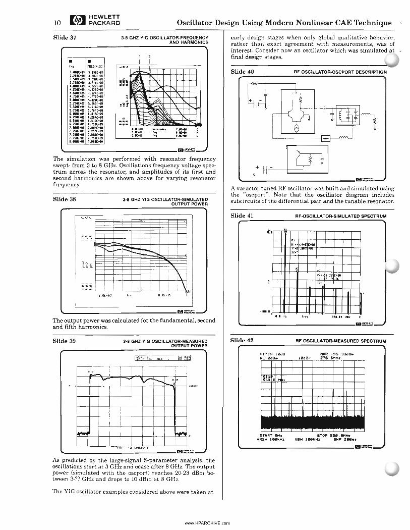
The simulation was performed with resonator frequencyswept- from 3 to 8 GHz. Oscillations frequency voltage spectrum across the resonator, and amplitudes of its first andsecond harmonics are shown above for varying resonatorfrequency.
RF OSCILLATOR-oSCPORT DESCRIPTION
'- liJ=
Slide 40
A varactor-tuned RF oscillator was built and simulated usingthe "oscport". Note that the oscillator diagram includessubcircuits of the differential pair and the tunable resonator.
early design stages when only global qualitative behavior,rather than exact agreement with measurements, was ofinterest. Consider now an oscillator which was simulated at •fmal design stages.
-----------J
7.....,.11:"......1.11:"
3.1£..1....
3-8 GHZ YIG OSCILLATOR·SIMULATEDOUTPUT POWER
3-8 GHZ YIG OSCILLATOR·FREQUENCYAND HARMONICS
• •"q nEO(.,2)
1._'" 1.1lIl:.e5l.lSI[.., 1.2IX'"1._'" 1.531['"1.1$1['" 1.171['"4'-'" 4.117['"4.251(.., 4.215('"4._'" 4.5241:'"4.1$1['" 4.172['"5._'" 5.1111:'"5.2511:'" 5.2U(..,5._'" 5.5,1[..,5.1$1[.., 5.717['"1._'" 1.115['"1.2511:'" 1.214['"1.5.'" 1.512['"1.1$1[.., I.15!lt..,7._'" 7•.-J('"7.2511:'" 7.255('"7._'" 7.93['"7.1$1['" 7.15'['"1._'" 7.t!!lt..,
Slide 37
Slide 38
Slide 41 RF-oSCILLATOR-SIMULATED SPECTRUM
"".""csicsics:i
--I ..... roo- '"I'\
1\
1\J.I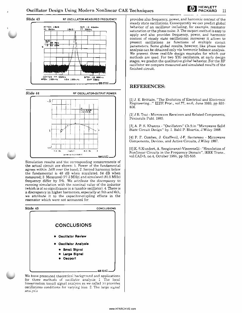
• Oscillator Design Using Modern Nonlinear CAE TechniquesF/;j;I HEWLETT 11~~ PACKARD
Slide 43 RF OSCILLATOR·MEASURED FREQUENCY
ATT£t< ll1d& "'<II -3 3 ...&.RL 8dS,. llild 8/ 77 3ilMHz
5 r--+-t--+--+-+++-+-~-+-1,----l
SPAt< lB._HzSWPSIiloo._________________M=
provides also frequency, power, and harmonic content of thesteady state oscillations. Consequently we can predict globalbehavior of an oscillator including, for example, resonatorsaturation or the phase noise. 3. The oscport method is easy toapply and also provides frequency, power, and harmoniccontent of steady state oscillations; moreover it allows topresent oscillations as functions of multiple circuitparameters. Some global results, however, like phase noiseanalysis can be obtained only via harmonic balance analysis.We present three real·life design examples for which ourmethods are used. For two YIG oscillators, at early designstages, we predict the qualitative global behavior. For the RFoscillator we compare measured and simulated results of thefinished circuit.
REFERENCES:Slide 44
-...RF OSCILLATOR-oUTPUT POWER
"..- ::M:~""
/ r---.-"V' I'- "
[1] J. E. Brittain, "The Evolution of Electrical and ElectronicEngineering..." IEEE Proc., vo!.77, no.6, June 1989, pp 837·856.
[2] J.B. Tsui - Microwave Receivers and Related Components,Peninsula Pub!. 1985.
[3} A. P. S. Khanna· "Oscillators" Ch.9.in "Microwave SolidState Circuit Design" by. I. Bahl P. Bhartia, J.wiley 1988.
....". ...1.....1' ••1)·111.111.
_________________M=
Simulation results and the corresponding measurements ofthe actual circuit are shown: 1. Power of the fundamentalagrees within .5dB over the band; 2. Second harmonic belowthe fundamental is 48 dB when simulated, 54 dB whenmeasured; 3. Measured (77.3 MHz) and simulated (81.0 MHz)frequency differ by 5%. We attribute the discrepancy torunning simulation with the nominal value of the inductor(which is of no significance in a tunable oscillator). 4. There isa discrepancy in higher harmonics, especially at 5th and 6th,we attribute it to the capacitor-coupling effects in theresonator which were not accounted for.
[4] P. F. Combes, J. Graffeuil, J-F. Sautereau - MicrowaveComponents, Devices, and Active Circuits, J.Wiley 1987.
[5] K. S.Kundert, A. Sangiovanni-Vincentelli - "Simulation ofNonlinear Circuits in the Frequency Domain", IEEE Trans.,vo!.CAD-5, no.4, October 1986, pp 521-535.
Slide 45
CONCLUSIONS
• Oaclllator Review
• Oacillator Analyala
• Small Signal• Large Signal• Oacport
CONCLUSIONS
_________________M=
We have presented theoretical background and applicationsfor three methods of oscillator analysis: 1. The locallinearization (small signal analysis as we called it) providesoscillations conditions for varying bias. 2. The large signalanalysis
www.HPARCHIVE.com

www.HPARCHIVE.com
FG'A HEWLETT~e. PACKARD
Copyright © 1990Hewlett-Packard CompanyPrinted in U.S.A. 41905952-2388
I