Embed Size (px)
Citation preview
Otolith Aging and Analysis
William T. Stewart
Computational Bioscience ProgramArizona State University
Internship advisors
Dr. Rosemary RenautDr. Paul Marsh
Arizona State University
Scott Byan Kirk Young
Marianne Meding
Arizona Game and Fish Department
report number 05-06
1
Table of Contents
Abstract...............................................................................................................................4Section 1..............................................................................................................................5Introduction........................................................................................................................5
1.1 Aging structures...........................................................................................51.2 Otoliths.........................................................................................................51.3 Annuli formation..........................................................................................61.4 Otolith preparation and interpretation..........................................................81.5 Important otolith features.............................................................................91.6
Objective......................................................................................................10Section 2............................................................................................................................11Materials and Methods....................................................................................................11
2.1 Image capturing.........................................................................................112.2 Image enhancement....................................................................................112.3 Counting and measuring annuli..................................................................122.4 Graphical user interface..............................................................................15
Section 3............................................................................................................................16Results...............................................................................................................................16
3.1 Image enhancement....................................................................................163.2 Manual count..............................................................................................193.3 Semi-automatic count.................................................................................213.4 Comparing the two approaches..................................................................233.5 Graphical user interface..............................................................................243.6 Help file......................................................................................................25
Section 4............................................................................................................................27Conclusion and Discussion..............................................................................................27
4.1 Final product..............................................................................................274.2 Problems.....................................................................................................274.3 Future work................................................................................................28
References.........................................................................................................................30
2

List of Figures and Tables
Figures
Figure 1 Otolith image with 6 annuli..........................................................................7Figure 2 Otolith image with reference to nucleus annuli and sulcus........................10Figure 3a Otolith image with profile line...................................................................13Figure 3b Profile plot of image 3a..............................................................................13Figure 4 Profile with linear fit and residuals............................................................14Figure 5a Otolith image with region of interest.........................................................15Figure 5b Region of interest with profile rays............................................................15Figure 6a Otolith image before enhancement.............................................................17Figure 6b Otolith image after enhancement...............................................................17Figure 7a Profile plot before enhancement.................................................................18Figure 7b Profile plot after enhancement...................................................................19Figure 8 Otolith image showing result of manual selection.....................................20Figure 9 Otolith image showing results of semi-automatic selection.......................22Figure 10 Comparison plot of annuli ratio from two different methods....................23Figure 11 Smapshot of graphical user interface.........................................................25
Tables
Table 1a Local min and max values of profile of non-ehnaced images....................17Table 1b Local min and max values of profile of ehnaced images...........................17Table 2 x and y coordinates of manual selection with intensities...........................21Table 3 Annuli ratios from manual method............................................................21Table 4 Annuli ratios from semiautomatic method.................................................22Table 5 Ratio comparison between to different methods........................................23
3
Abstract
Otoliths, also known as earstones are paired calcified structures used for balance and
hearing in teleost fish. An otolith is acellular and metabolically inert providing biologists
with a record of exposure to both the temperature and composition of the ambient water.
Otoliths provide an abundance of information ranging from temperature history, detection
of anadromy, determination of migration pathways, stock identification, use as a natural
tag, and most importantly age validation. Growth rings (annuli) on the otolith record the
age and growth of a fish from birth to death. With the use of Matlab the goal of this
project is to design a program that uses digital otolith images to semi-automate the aging
process. There are three main components to this task. The first is to clear up the image
making each annuli in the otolith distinct. The second is to count the number of annuli
from the focus of the otolith to the edge and measure distances between each annuli. The
third component is to use different backcalculation models to estimate a fish's length at
age n. Results from the image enhancement process greatly increased the contrast, which
in turn provided more accurate results for the semi-automatic aging approach. However,
this approach to aging decreases in accuarcy as the number of annuli increase. For this
reason a manual measurement was added to the program allowing the user to select each
annulus simply by clicking on it. For fish with five or less annuli the semi-automatic and
manual methods have the same accuracy. The otolith aging outputs for this program are
annuli estimate, number of rays, distance from the nucleus to each annulus and the edge,
and standard deviation.
4
Section 1
Introduction
1.1
Aging structures
Fish age and size are two of the most important pieces of biological data found in
fisheries research. It is the foundation on which fisheries management is built. With this
information biologists can infer about population, growth rates, age specific estimates of
stock biomass, mortality rates and predictions of future stock conditions. Biologists can
use several different structures within the fish to acquire information regarding fish age.
These structures include scales, fin rays, vertebrae, and most importantly otoliths. Scales
can be difficult to read due to resorbtion. The benefit of scales, unlike other structures, is
that samples can be taken without having to kill the fish. Fin rays to some extent can also
be collected without mortality. While otolith collection requires killing the fish, this is
the most widely used strucutre. The reason being, they generally are almost always
easiest to read. Often times several structures are used to achieve the most accurate aging
results.
1.2
Otoliths
Otoliths sometimes called earstones are hard calcified carbonate structures located
in the brain casing of all teleost fish. Fish use them for hearing and balance, but
biologists use them for aging and growth studies. Otoliths are popular because compared
5
to other structure they generally provide the most accurate ages, mainly due to their
continued growth throughout the life of the fish. Otoliths are acellular which, implies
that they are not subject to resorption. This gives them an advantage over aging scales.
Each fish has three types of otoliths; sagittae astericii, and lapilli. Sagittae are the largest
and most commonly used for aging. The sagittae are involved in the detection of sound,
converting sound waves into electrical signals. Asteriscii, which are smaller than the
sagittae, are also involved in the detection of sound. If accurate ages can not be estimated
using the sagittae it is not uncommon to use the asteriscii as backup. Finally the lapilli,
usually the smallest of the three pairs of otoliths, are used for the detection of
gravitational force and sound. (Popper and Lu 2000). The lapilli are hardly ever used for
aging
Otoliths vary in shape and size depending on the species. Researchers who
analyze stomach contents occasionally use otolith shape to help identify fish species. In
addition, other studies have shown otoliths being used to record temperature history
(Patterson et al. 1993), whether a fish is anadromous (Secor 1992), migration pathways
(Thresher et. al. 1994), stock identification (Edmonds et. al. 1989), or have been used as a
natural tag (Campana et. al. 1995).
1.3
Annuli formation
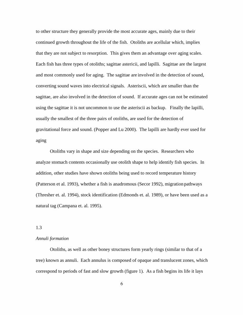
Otoliths, as well as other boney structures form yearly rings (similar to that of a
tree) known as annuli. Each annulus is composed of opaque and translucent zones, which
correspond to periods of fast and slow growth (figure 1). As a fish begins its life it lays
6
down daily rings as a result of an internal clock which is entrained by a 24-hour light and
dark cycle. In addition environmental factors such as feeding, activity and temperature
variations all contribute to the daily cycle (Campana and Neilson, 1985). During periods
of slow growth daily rings form extremely close together creating a thick band or annulus.
In general, the opaque zone forms during periods of increasing water temperatures, while
the translucent zone is formed during periods of reduced growth which may be associated
with spawning. The formation of annuli is not always clear cut. Unusual weather may
provide a period of increased food resources during otherwise poor conditions. This
could result in a temporary period of fast growth which might leave an impression of a
false annulus.
Figure 1.This was taken from a cod that has six annuli. Each annuli is indicated by arrows.Courtesy of Otolith research laboratory Bedford institute of Oceanography.
7
1.4
Otolith preparation and interpretation
Otolith preparation is a very time consuming process. It requires a microscope
slide, some type of thermoplastic glue, and a means to section the otolith either by
grinding with sand paper or a diamond blade wet saw. The idea is to grind the otolith
from either side until a thin section containing the nucleus remains. Depending on a
person's experience this can take up to an hour. Once this is completed the sectioned
otolith is mounted onto a slide then read by an experienced technician.
Upon completion of otolith interpretation a reader must then measure the distance
between annuli in order to perform a backcalculation. Backcalculations estimate the
fish's length at a previous age. The reader determines the ratio between otolith length and
fish length. For example if the relationship is linear than the increment width between
annuli are proportional to the growth of the fish. There are several models used to
describe this relationship. One of the traditional models is the Fraser-Lee, which is
similar to a linear regression model. However, most species otolith:fish length
relationships are not exactly linear. A number of studies have shown that otoliths of slow
growing fish are generally larger and heavier than those of fast growing fish of the same
size. To account for the difference in growth rate, the biological intercept model was
created. Similar to the Fraser-Lee model, this model assumes a linear relationship, but
adds a biological intercept that is determined by the mean size of the fish and otolith at
the larval or juvenile stage (Campana and Jones 1992). A third approach is the Weisburg
model. This approach uses a linear model to separate age and year specific effect on
otolith growth similar to a two-way analysis of variance (Klumb et. al. 2001). The model
8
accounts for environmental influences. When choosing the best model, it is important to
understand something about the life history of the species in question.
1.5
Important otolith features
When analyzing images, there are a few important features that must be noted.
Annuli are generally oriented parallel to the outer surface of the otolith. They surround
the core or nucleus which in most cases is translucent. Near the core is the sulcus which
is a longitudinal groove through which an auditory nerve passes. Many times annuli are
most clear near the sulcus (figure 2). Interpretation of otoliths takes a lot of practice.
Depending on the experience of the technician there are a wide variety of problems
associated with preparation. Improperly prepared otoliths can result in the absence of
annuli. In many cases abnormal periods of rapid growth caused by unusual
environmental conditions can create splits in annuli or even perhaps a false annulus. The
first annulus in figure 2 shows an example of a split.
9
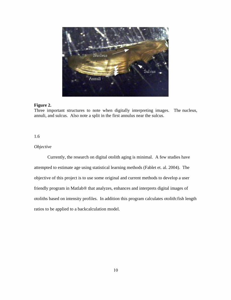
Figure 2. Three important structures to note when digitally interpreting images. The nucleus,annuli, and sulcus. Also note a split in the first annulus near the sulcus.
1.6
Objective
Currently, the research on digital otolith aging is minimal. A few studies have
attempted to estimate age using statistical learning methods (Fablet et. al. 2004). The
objective of this project is to use some original and current methods to develop a user
friendly program in Matlab® that analyzes, enhances and interprets digital images of
otoliths based on intensity profiles. In addition this program calculates otolith:fish length
ratios to be applied to a backcalculation model.
10
Section 2
Materials and Methods
2.1
Image capturing
Images are from already prepared otoliths of largemouth bass (Micropterus
salmoides), white bass (Morone chrysops) and striped bass (Morone saxatilis) collected
from Lake Pleasant just north of Phoenix Arizona. A digital camera attached to a light
microscope was used to capture images. Xcap, an image capturing software was used to
collect the images that were then analyzed using Matlab 7 (R14)®.
2.2
Image enhancement
The first step was to read the image into the program and change the image from a
colormap to a grayscale intensity image. A contrast limited adaptive histogram
equalization (CLAHE) was the method used to enhance the image. The contrast of the
image is enhanced by transforming the intensity values using CLAHE. The image is
subdivided into nXm blocks or tiles. The tiles are specified by the user prior to
enhancement. Each tile's contrast is enhanced so that the histogram of the output region
approximately matches a flat histogram. The minimum and maximum tile range is 2 X 2
and 50 X 50 respectively.
11
2.3
Counting and measuring annuli
To measure annuli the program is designed to allow the user to select a manual or
semi-automatic approach to counting. The impixel function is used for manual
measurement. Impixel allows the user to select points on an image returning the
coordinates as well as the intensity value of each point. Once all selections are made, the
number of points are counted and distances are between points are measured. The
distances between each annuli are applied to one of several backcalculations to establish
length at age of an individual fish.
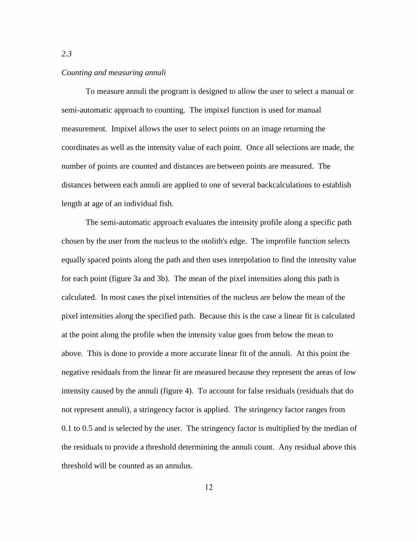
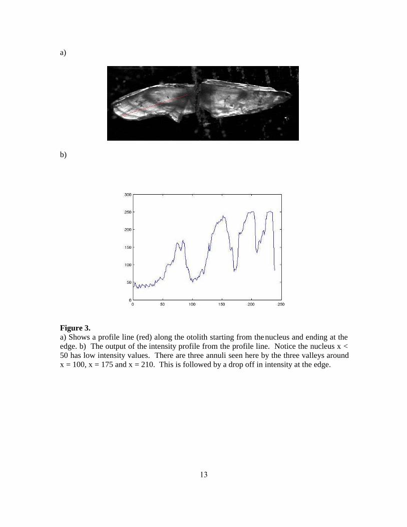
The semi-automatic approach evaluates the intensity profile along a specific path
chosen by the user from the nucleus to the otolith's edge. The improfile function selects
equally spaced points along the path and then uses interpolation to find the intensity value
for each point (figure 3a and 3b). The mean of the pixel intensities along this path is
calculated. In most cases the pixel intensities of the nucleus are below the mean of the
pixel intensities along the specified path. Because this is the case a linear fit is calculated
at the point along the profile when the intensity value goes from below the mean to
above. This is done to provide a more accurate linear fit of the annuli. At this point the
negative residuals from the linear fit are measured because they represent the areas of low
intensity caused by the annuli (figure 4). To account for false residuals (residuals that do
not represent annuli), a stringency factor is applied. The stringency factor ranges from
0.1 to 0.5 and is selected by the user. The stringency factor is multiplied by the median of
the residuals to provide a threshold determining the annuli count. Any residual above this
threshold will be counted as an annulus.
12
a)
b)
Figure 3. a) Shows a profile line (red) along the otolith starting from the nucleus and ending at theedge. b) The output of the intensity profile from the profile line. Notice the nucleus x <50 has low intensity values. There are three annuli seen here by the three valleys aroundx = 100, x = 175 and x = 210. This is followed by a drop off in intensity at the edge.
13
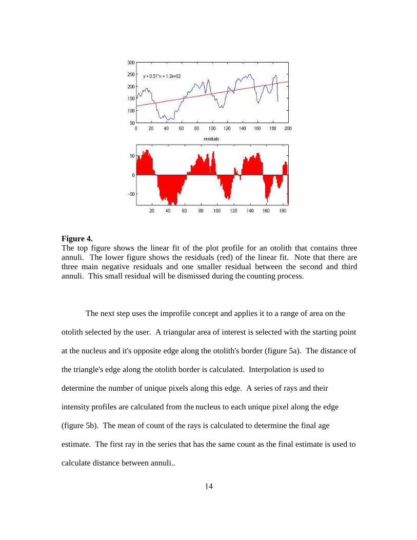
Figure 4.The top figure shows the linear fit of the plot profile for an otolith that contains threeannuli. The lower figure shows the residuals (red) of the linear fit. Note that there arethree main negative residuals and one smaller residual between the second and thirdannuli. This small residual will be dismissed during the counting process.
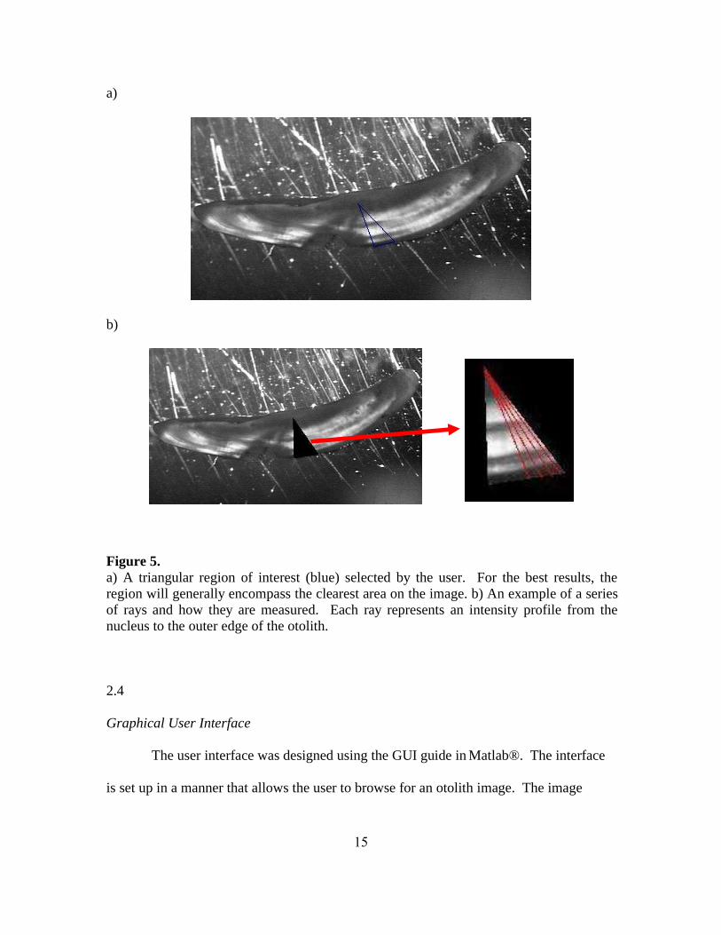
The next step uses the improfile concept and applies it to a range of area on the
otolith selected by the user. A triangular area of interest is selected with the starting point
at the nucleus and it's opposite edge along the otolith's border (figure 5a). The distance of
the triangle's edge along the otolith border is calculated. Interpolation is used to
determine the number of unique pixels along this edge. A series of rays and their
intensity profiles are calculated from the nucleus to each unique pixel along the edge
(figure 5b). The mean of count of the rays is calculated to determine the final age
estimate. The first ray in the series that has the same count as the final estimate is used to
calculate distance between annuli..
14
a)
b)
Figure 5. a) A triangular region of interest (blue) selected by the user. For the best results, theregion will generally encompass the clearest area on the image. b) An example of a seriesof rays and how they are measured. Each ray represents an intensity profile from thenucleus to the outer edge of the otolith.
2.4
Graphical User Interface
The user interface was designed using the GUI guide in Matlab®. The interface
is set up in a manner that allows the user to browse for an otolith image. The image
15
appears on the right hand side of the window. A radio button lets the user choose
between a manual measurement or a semi-automatic measurement. A slider called
enhancement was created allowing the user to select the value of the nXm matrix for the
histogram equalization. When the enhancement button is push the image is updated in its
enhanced form. Another slider can be adjusted to select the stringency factor. On the
lower left hand corner of the screen is the output, which provides the results of the
estimation of annuli, number of rays used in the estimation, standard deviation, and the
distances between annuli. In addition a fish size text box allows the user to type in the
size of the fish for backcalculation purposes. A yellow x is used to mark each annulus
and the outer edge. A red x is used to identify the nucleus of the otolith.
Section 3
Results
3.1
Image enhancement
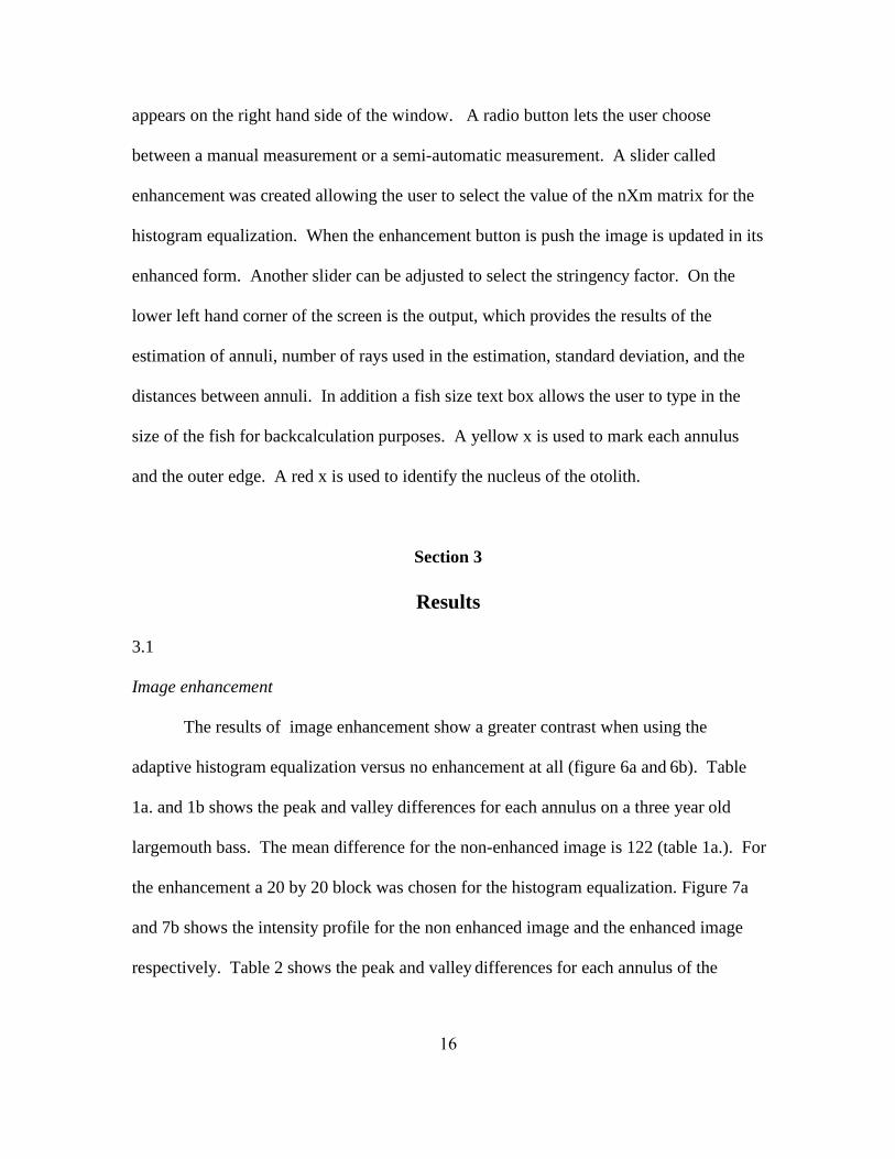
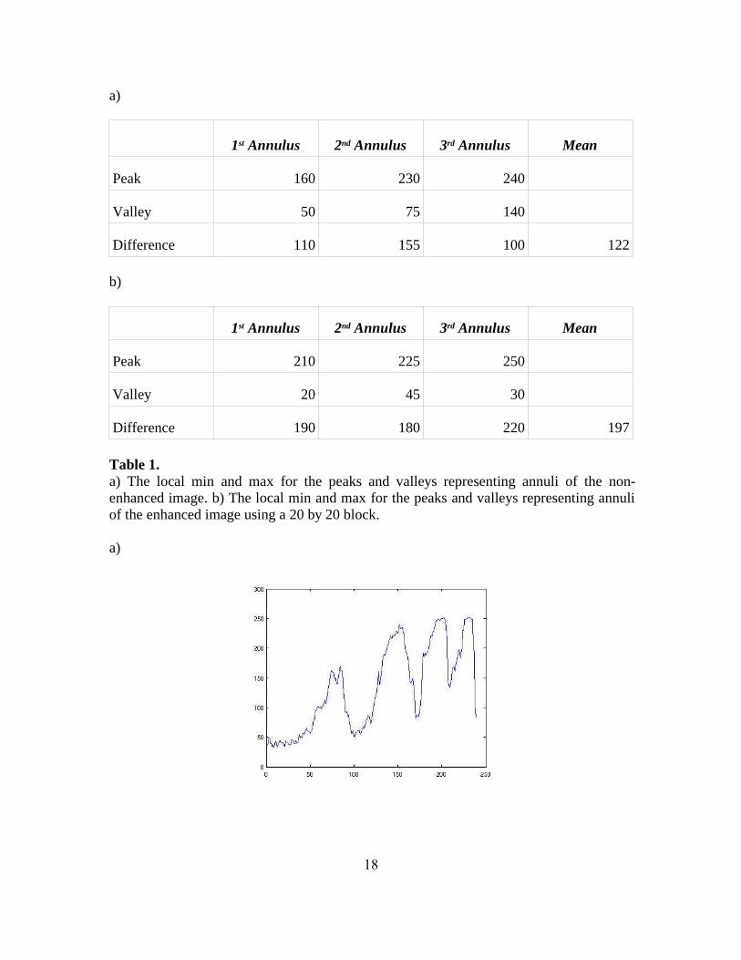
The results of image enhancement show a greater contrast when using the
adaptive histogram equalization versus no enhancement at all (figure 6a and 6b). Table
1a. and 1b shows the peak and valley differences for each annulus on a three year old
largemouth bass. The mean difference for the non-enhanced image is 122 (table 1a.). For
the enhancement a 20 by 20 block was chosen for the histogram equalization. Figure 7a
and 7b shows the intensity profile for the non enhanced image and the enhanced image
respectively. Table 2 shows the peak and valley differences for each annulus of the
16
enhanced image. The mean difference for the enhanced image is 197 (table 1b). The
enhancement difference between images is 75. The results also showed the number of
residuals increased with image enhancement. The residuals however were factored out
when the stringency factor was applied.
a)
b)
Figure 6. a) A three year old largemouth bass before image enhancement. b) The same image as a)after image enhancement. To enhance this image a 20 by 20 block was used for theimage histogram equalization.
17
a)
1st Annulus 2nd Annulus 3rd Annulus Mean
Peak 160 230 240
Valley 50 75 140
Difference 110 155 100 122
b)
1st Annulus 2nd Annulus 3rd Annulus Mean
Peak 210 225 250
Valley 20 45 30
Difference 190 180 220 197
Table 1. a) The local min and max for the peaks and valleys representing annuli of the non-enhanced image. b) The local min and max for the peaks and valleys representing annuliof the enhanced image using a 20 by 20 block.
a)
18
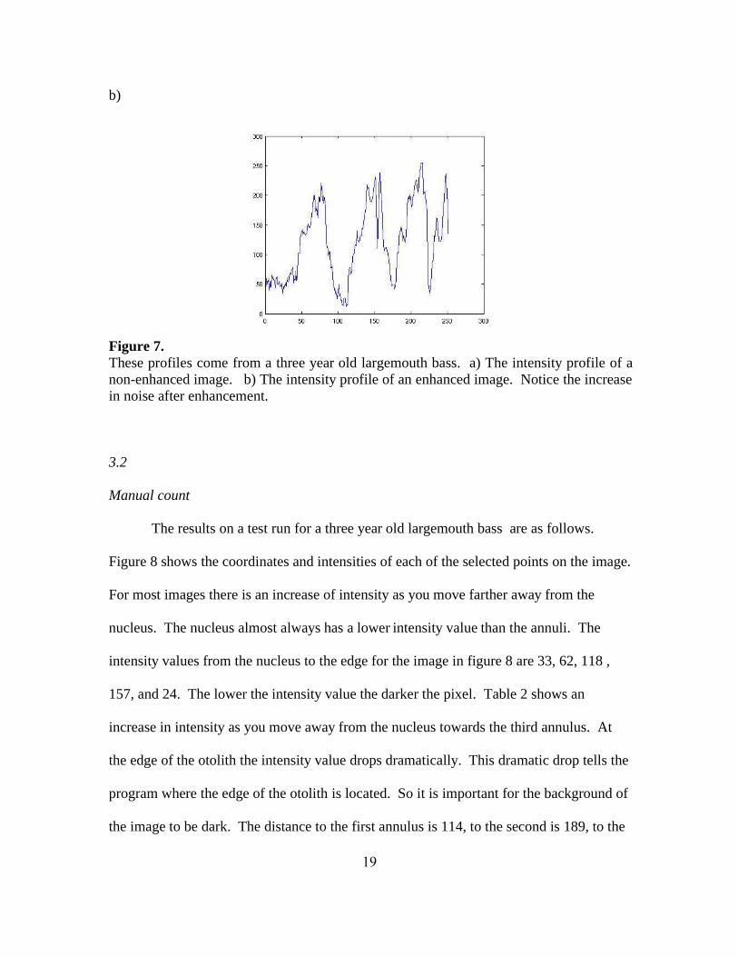
b)
Figure 7. These profiles come from a three year old largemouth bass. a) The intensity profile of anon-enhanced image. b) The intensity profile of an enhanced image. Notice the increasein noise after enhancement.
3.2
Manual count
The results on a test run for a three year old largemouth bass are as follows.
Figure 8 shows the coordinates and intensities of each of the selected points on the image.
For most images there is an increase of intensity as you move farther away from the
nucleus. The nucleus almost always has a lower intensity value than the annuli. The
intensity values from the nucleus to the edge for the image in figure 8 are 33, 62, 118 ,
157, and 24. The lower the intensity value the darker the pixel. Table 2 shows an
increase in intensity as you move away from the nucleus towards the third annulus. At
the edge of the otolith the intensity value drops dramatically. This dramatic drop tells the
program where the edge of the otolith is located. So it is important for the background of
the image to be dark. The distance to the first annulus is 114, to the second is 189, to the
19
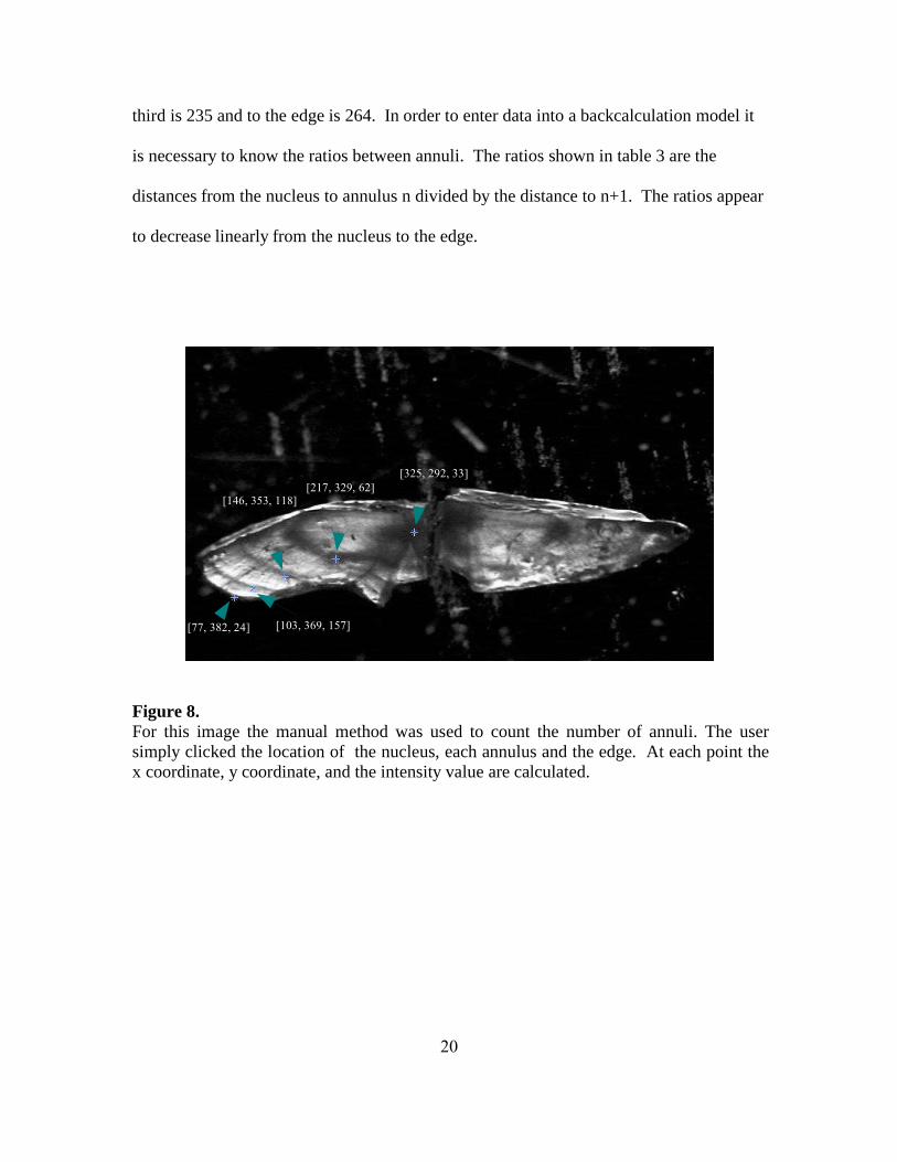
third is 235 and to the edge is 264. In order to enter data into a backcalculation model it
is necessary to know the ratios between annuli. The ratios shown in table 3 are the
distances from the nucleus to annulus n divided by the distance to n+1. The ratios appear
to decrease linearly from the nucleus to the edge.
Figure 8. For this image the manual method was used to count the number of annuli. The usersimply clicked the location of the nucleus, each annulus and the edge. At each point thex coordinate, y coordinate, and the intensity value are calculated.
20
[77, 382, 24]
[325, 292, 33]
[103, 369, 157]
[146, 353, 118][217, 329, 62]
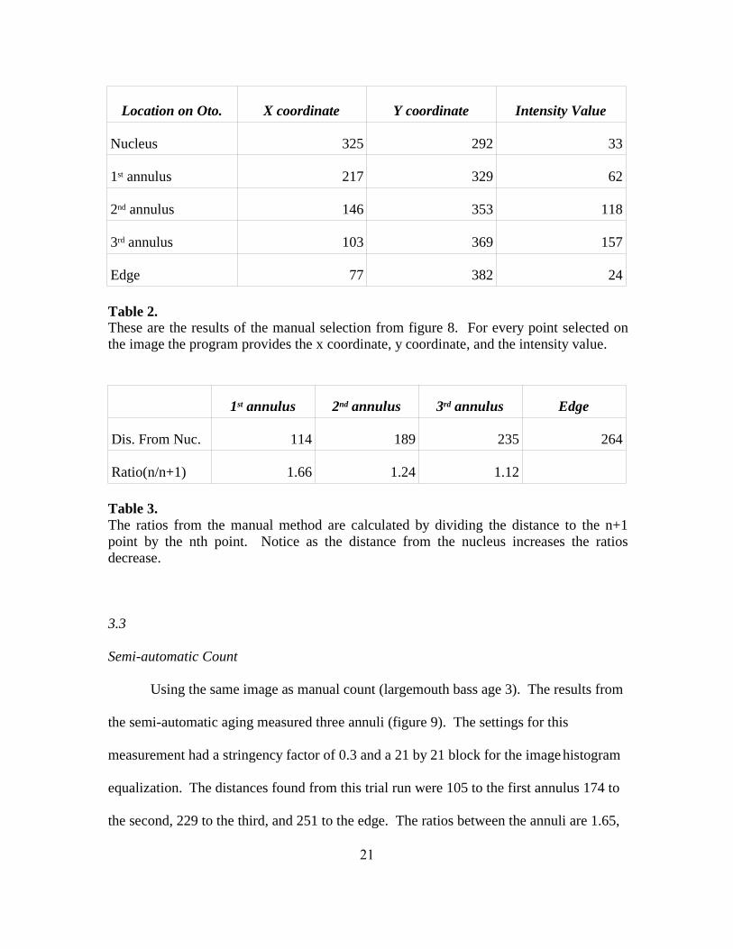
Location on Oto. X coordinate Y coordinate Intensity Value
Nucleus 325 292 33
1st annulus 217 329 62
2nd annulus 146 353 118
3rd annulus 103 369 157
Edge 77 382 24
Table 2.These are the results of the manual selection from figure 8. For every point selected onthe image the program provides the x coordinate, y coordinate, and the intensity value.
1st annulus 2nd annulus 3rd annulus Edge
Dis. From Nuc. 114 189 235 264
Ratio(n/n+1) 1.66 1.24 1.12
Table 3. The ratios from the manual method are calculated by dividing the distance to the n+1point by the nth point. Notice as the distance from the nucleus increases the ratiosdecrease.
3.3
Semi-automatic Count
Using the same image as manual count (largemouth bass age 3). The results from
the semi-automatic aging measured three annuli (figure 9). The settings for this
measurement had a stringency factor of 0.3 and a 21 by 21 block for the image histogram
equalization. The distances found from this trial run were 105 to the first annulus 174 to
the second, 229 to the third, and 251 to the edge. The ratios between the annuli are 1.65,
21
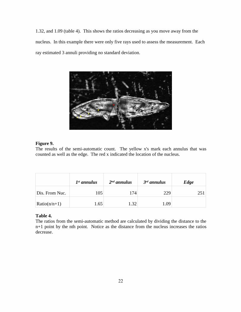
1.32, and 1.09 (table 4). This shows the ratios decreasing as you move away from the
nucleus. In this example there were only five rays used to assess the measurement. Each
ray estimated 3 annuli providing no standard deviation.
Figure 9. The results of the semi-automatic count. The yellow x's mark each annulus that wascounted as well as the edge. The red x indicated the location of the nucleus.
1st annulus 2nd annulus 3rd annulus Edge
Dis. From Nuc. 105 174 229 251
Ratio(n/n+1) 1.65 1.32 1.09
Table 4. The ratios from the semi-automatic method are calculated by dividing the distance to then+1 point by the nth point. Notice as the distance from the nucleus increases the ratiosdecrease.
22
3.4
Comparing the two approaches
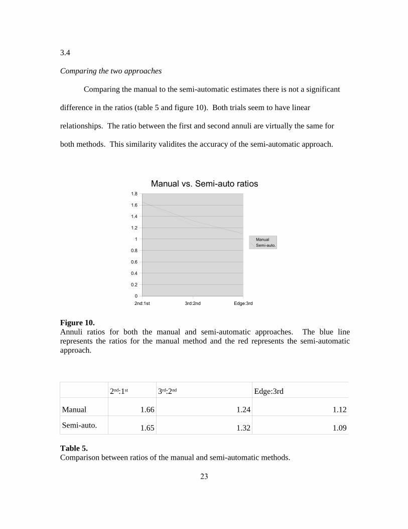
Comparing the manual to the semi-automatic estimates there is not a significant
difference in the ratios (table 5 and figure 10). Both trials seem to have linear
relationships. The ratio between the first and second annuli are virtually the same for
both methods. This similarity validites the accuracy of the semi-automatic approach.
2nd:1st 3rd:2nd Edge:3rd0
0.2
0.4
0.6
0.8
1
1.2
1.4
1.6
1.8
Manual vs. Semi-auto ratios
ManualSemi-auto.
Figure 10. Annuli ratios for both the manual and semi-automatic approaches. The blue linerepresents the ratios for the manual method and the red represents the semi-automaticapproach.
2nd:1st 3rd:2nd Edge:3rd
Manual 1.66 1.24 1.12
Semi-auto. 1.65 1.32 1.09
Table 5. Comparison between ratios of the manual and semi-automatic methods.
23
3.5
Graphical User Interface
This final product is an easy to use graphical interface. Figure 11 shows a
screenshot of the interface. The user simply browses for the the image of interest and
loads it onto the screen. Once the image appears the user can make adjustments as
needed. Each adjustment can be monitored every time the user clicks on the adjust image
button. The default is for the program to semi-automate the count process. When the
image is adjusted correctly the user can then select the manual count radio button to
manually measure the image. If the image looks to have a lot of noise the stringency
factor can also be adjusted prior to measuring. When everything is adjusted, the user
simply clicks the measure button and then measures a triangular area of interest. The
results are displayed showing the distances, number of rays used, final count, and
standard deviation.
24
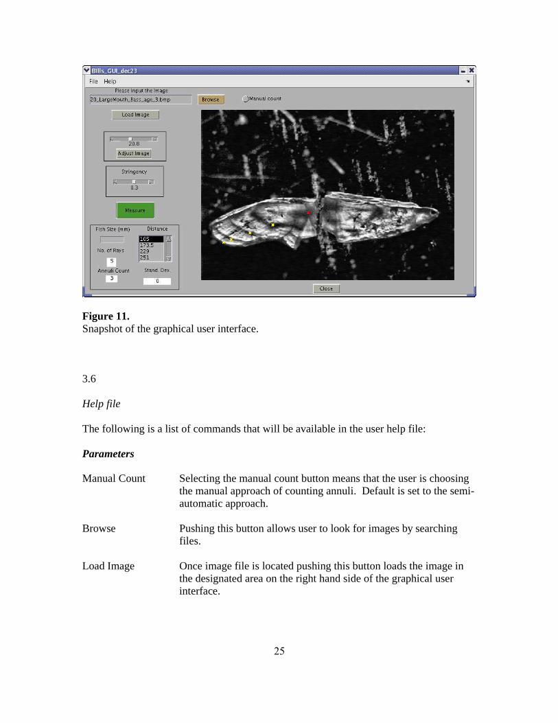
Figure 11. Snapshot of the graphical user interface.
3.6
Help file
The following is a list of commands that will be available in the user help file:
Parameters
Manual Count Selecting the manual count button means that the user is choosing the manual approach of counting annuli. Default is set to the semi-automatic approach.
Browse Pushing this button allows user to look for images by searching files.
Load Image Once image file is located pushing this button loads the image in the designated area on the right hand side of the graphical user interface.
25
Adjust image Pressing this button adjusts and updates the image using an adaptive histogram equilization technique. The range is from two to fifty. The higher the number the more contrasted the image.
Stringency Adjusting this slider changes how stringent the counting process will be for the semi-automatic approach. The range is from 0.1 ot 0.5. When there is a large amount of image noise, increasing the stringency will help reduce the possiblity of counting false annuli. Default is set to 0.3. The adjustments will not take effect until the meaure button is pressed.
Measure Once all adjustments are made pressing the measure button will estimate age and determine distance between annuli.
Close This button closes the program.
Output
Distance This is the distance from the nucleus to each annulus and the edge.The last number will always be the edge.
Fish size This box is where the user enters the size of the fish in millimeters.This will later be used for backcalculation.
No. of rays The number is this box indicates the number of rays used to estimate the annuli count. Used only in the semi-automatic approach.
Annuli count This box shows the result of annuli estimation.
Stand. Dev. This box shows the standard deviation of the annuli estimation. For the semi-automatic approach only.
26
Section 4
Conclusion and Discussion
4.1
Final product
The purpose of this project was to design an easy to use program that would count
annuli and measure the annuli ratios. This would help eliminate the headache of having
to manually measure distances using an outdated program or even having to physically
measure distances under a microscope. With software tools such as Matlab® it is easy to
take this one step farther by adding image enhancement properties.
What was initially intended for this program and is actually useful changed during
it's creation. Initially this was designed to get an accurate age estimation by analyzing the
image. While this program does come up with an estimate it really is no faster than
having a reader look at the otolith under a microscope and physically count the annuli.
The features that make this program very useful to biologists are the distance ratios. The
simplicity of either clicking on the annuli or selecting an area of interest drastically
decreases the time needed to find such ratios.
4.2
Problems
Over the course of this project a number of problems occurred. The equipment
used to capture the images created much noise surrounding the otolith, which is why
image histogram equalization worked so much better than the a regular histogram
27
equalization. As mentioned earlier the image histogram equalization only equalizes in a
specified area. If the image capturing equipment was improved perhaps an even more
contrasted image would result. With better quality images more of the background noise
would be removed. If one could altogether eliminate background noise there are a
number of image enhancement techniques that can be applied. For example an edge
detection could help isolate the image followed by the use of a series of filters which
could leave an image only containing annuli.
The semi-automatic approach by no means is completely accurate especially when
there is a lot of noise. An important feature is the yellow and red marks which tell the
user where the program calculated either the annuli, the edge, or the nucleus. If the marks
are not over any of these features of the otolith it is very simple to remeasure. The marks
insure that the estimates are accurate.
Another problem arises with older aged fish. As the number of annuli increases
the accuracy of the the program decreases. Part of this is due to the quality of the image.
When annuli appear to be closer together it is difficult for the program to distinguish
between annuli. That is the reason for the manual count. Again with improved
enhancement methods perhaps the semi-automatic approach would increase the accuracy
of aging older fish.
4.3
The future
There is still a large amount of work yet to be done with this aging program before
it can be used commercially. Currently there is a simple help file that will need to be
28
extended. In addition the creation of an option that allows the user to select a
backcalculation model to analyze the fish length:otolith ratios. A database will be
established containing the output of the results along with the image. The records could
be attached to the file name of the image so that multiple measures of the same image are
filed under the same record.
The amount of uses for image analysis in the enviromental field are endless. For
example otoliths are also used for the identification of species found in the stomach of
marine mammals. Identification based on shape analysis could be yet another project.
Beyond otoliths scientists are using geographical information systems to estimate
amounts of vegitation by analyzing areal photographs. Jaw images of mammals are used
to identify species by meauring suture distances. As technology advances image analysis
will begin to play an even larger role in the environmental sciences.
29
References
Branzer JC, Campana SE, Tanner DK (2004) Habitat Fingerprints for Lake Superior Coastal Wetlands Derived from Elemental Analysis of Yellow Perch Otoliths. Transactions of the American Fisheries Society 133:692–704
Campana, SE (1999) Chemistry and Composition of Fish Otoliths: pathways, mechanisms and applications REVIEW. Mar. Ecol. Prog. Ser.188:263-297
Campana SE, Gagne JA, McLaren JW (1995) Elemental Fingerprinting of Fish Otoliths Using ID-ICPMS. Mar. Ecol. Prog. Ser. 122:115-120
Campana, SE and Jones C. 1992. Analysis of otolith microstructure data. P. 73-100. In: D.K. Stevenson and S.E. Campana [eds]. Otolith microstructure examination and analysis. Can. Spec. Publ. Fish. Aquat. Sci. 117
Campana, SE and Neilson JD 1985. Microsturcutre of fish otoliths. Can. J. Fish. Aquat. Sci. 42:1014-1032
Dwyer KS, Walsh SJ, and Campana SE (2003) Age Determination, Validation and Growth of Grand Bank Yellowtail Flounder (Limanda ferruginea). ICES Journal of MarineScience. 60:1123–1138
Edmonds JS, Moran MJ, Caputi N, Morita M (1989) Trace Element Analysis of Fish Sagittae as an Aid to Stock Identification: Pink Snapper (Chrysophrys auratus) in Western Australia Waters. Can. J. Fish. Aquat. Sci. 46:50-54
Fablet R, Le Josse N, Benzinou, A (2004) Automated Fish Age Estimation From Otolith Images Using Statistical Learning. ICPR 4:503-506
Francis C, Campana SE (2004) Inferring Age From Otolith Measurements: A Review anda New Approach. Can. J. Fish. Aquat. Sci. 61: 1269-1284
Klumb RA, Bozek MA, Frie RV (2001)Validation of Three Back-calculation Models by Using Multiple Oxytetracycline Marks Formed in the Otoliths and Scales of Bluegill × Green Sunfish Hybrids. Can. J. Fish. Aquat. Sci. 58: 352–364
Patterson WP, Simth GR, Lohmann KC (1993) Contintental Paleothermometry and Seasonality Using the Isotopic Composition of Aragonitic Otoliths of Freshwater Fishes. Geophys. Mono. 78:191-202
30

Secor DH (1992) Application of Otolith Microchemistry Analysis to Investigate Anadromy n Chesapeake Bay striped bass Morone saxatilis. Fish. Bull., U.S. 90:798-806
Thorrold SR, Campana SE, Jones CM, Swart PK (1997) Factors Determining ?13C and
?18 O Fractionation in Aragonitic Otoliths of Marine Fish. Geochimica et Cosmochimica Acta. 61:2909-2919
Tresher RE, Proctor Ch, Gunn JS, Harrowfield IR (1994) An Evaluation of Electron Probe Microanalysis of Otoliths for Stock Delineation and Identification of Nursery Areas in a Southern Temperate Groundfish. Nemadactylus macropterus (Cheilodactylidae). Fish. Bull. 92:817-840
Mathworks website: http://www.mathworks.com
Otolith Research Laboratory Bedford Institute of Oceanography: http://www.mar.dfo-mpo.gc.ca/science/mfd/otolith/english/home.htm
31