1

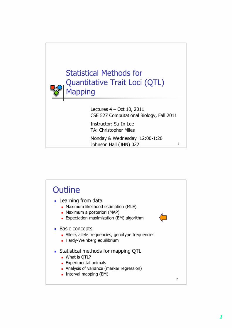
Lectures 4 – Oct 10, 2011CSE 527 Computational Biology, Fall 2011

Instructor: Su-In LeeTA: Christopher Miles

Monday & Wednesday 12:00-1:20Johnson Hall (JHN) 022

Statistical Methods for Quantitative Trait Loci (QTL) Mapping

1

2

Outline Learning from data

Maximum likelihood estimation (MLE) Maximum a posteriori (MAP) Expectation-maximization (EM) algorithm

Basic concepts Allele, allele frequencies, genotype frequencies Hardy-Weinberg equilibrium

Statistical methods for mapping QTL What is QTL? Experimental animals Analysis of variance (marker regression) Interval mapping (EM)

2

3

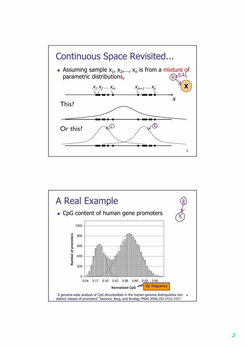
Continuous Space Revisited... Assuming sample x1, x2,…, xn is from a mixture of

parametric distributions,

x

x1 x2 … xm xm+1 … xn X

4

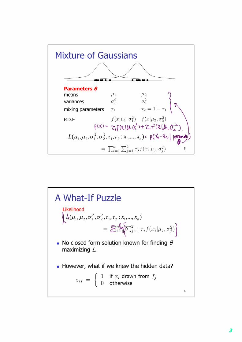
A Real Example CpG content of human gene promoters

“A genome-wide analysis of CpG dinucleotides in the human genome distinguishes twodistinct classes of promoters” Saxonov, Berg, and Brutlag, PNAS 2006;103:1412-1417

GC frequency

3

5

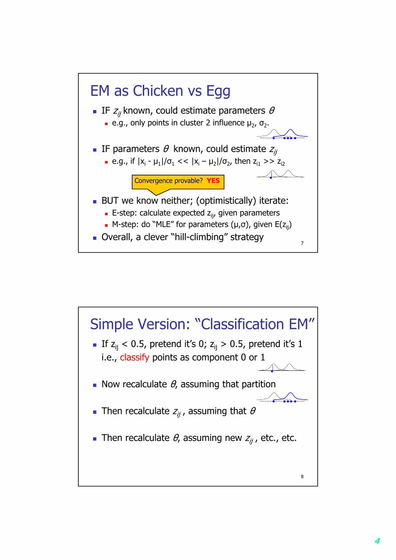
Mixture of Gaussians

Parameters θmeans variances

mixing parameters

P.D.F

),...,:,,,,,( 12122

2121 nxxL

6

A What-If Puzzle

No closed form solution known for finding θmaximizing L.

However, what if we knew the hidden data?

),...,:,,,,,( 12122

2121 nxxL

Likelihood

4

7

EM as Chicken vs Egg IF zij known, could estimate parameters θ

e.g., only points in cluster 2 influence μ2, σ2.

IF parameters θ known, could estimate zij e.g., if |xi - μ1|/σ1 << |xi – μ2|/σ2, then zi1 >> zi2

BUT we know neither; (optimistically) iterate: E-step: calculate expected zij, given parameters M-step: do “MLE” for parameters (μ,σ), given E(zij)

Overall, a clever “hill-climbing” strategy

Convergence provable? YES

8

Simple Version: “Classification EM” If zij < 0.5, pretend it’s 0; zij > 0.5, pretend it’s 1

i.e., classify points as component 0 or 1

Now recalculate θ, assuming that partition

Then recalculate zij , assuming that θ

Then recalculate θ, assuming new zij , etc., etc.

5

9

EM summary Fundamentally an MLE problem

EM steps E-step: calculate expected zij, given parameters M-step: do “MLE” for parameters (μ,σ), given E(zij)

EM is guaranteed to increase likelihood with every E-M iteration, hence will converge.

But may converge to local, not global, max.

Nevertheless, widely used, often effective

Outline Basic concepts

Allele, allele frequencies, genotype frequencies Hardy-Weinberg equilibrium

Statistical methods for mapping QTL What is QTL? Experimental animals Analysis of variance (marker regression) Interval mapping (Expectation Maximization)

10

6

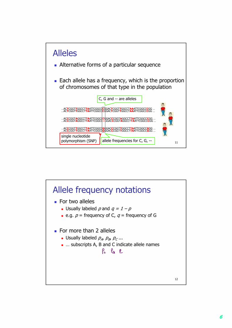
Alleles Alternative forms of a particular sequence

Each allele has a frequency, which is the proportion of chromosomes of that type in the population

11

…ACTCGGTTGGCCTTAATTCGGCCCGGACTCGGTTGGCCTAAATTCGGCCCGG …

…ACCCGGTAGGCCTTAATTCGGCCCGGACCCGGTAGGCCTTAATTCGGCCCGG …

…ACCCGGTTGGCCTTAATTCGGCCGGGACCCGGTTGGCCTTAATTCGGCCGGG …

…ACTCGGTTGGCCTTAATTCGGCCCGGACTCGGTTGGCCTAAATTCGGCCCGG …

…ACCCGGTAGGCCTTAATTCGGCC--GGACCCGGTAGGCCTTAATTCGGCCCGG …

…ACCCGGTTGGCCTTAATTCGGCCGGGACCCGGTTGGCCTTAATTCGGCCGGG …

C, G and -- are alleles

allele frequencies for C, G, --single nucleotide polymorphism (SNP)

Allele frequency notations For two alleles

Usually labeled p and q = 1 – p e.g. p = frequency of C, q = frequency of G

For more than 2 alleles Usually labeled pA, pB, pC ... … subscripts A, B and C indicate allele names

12

7

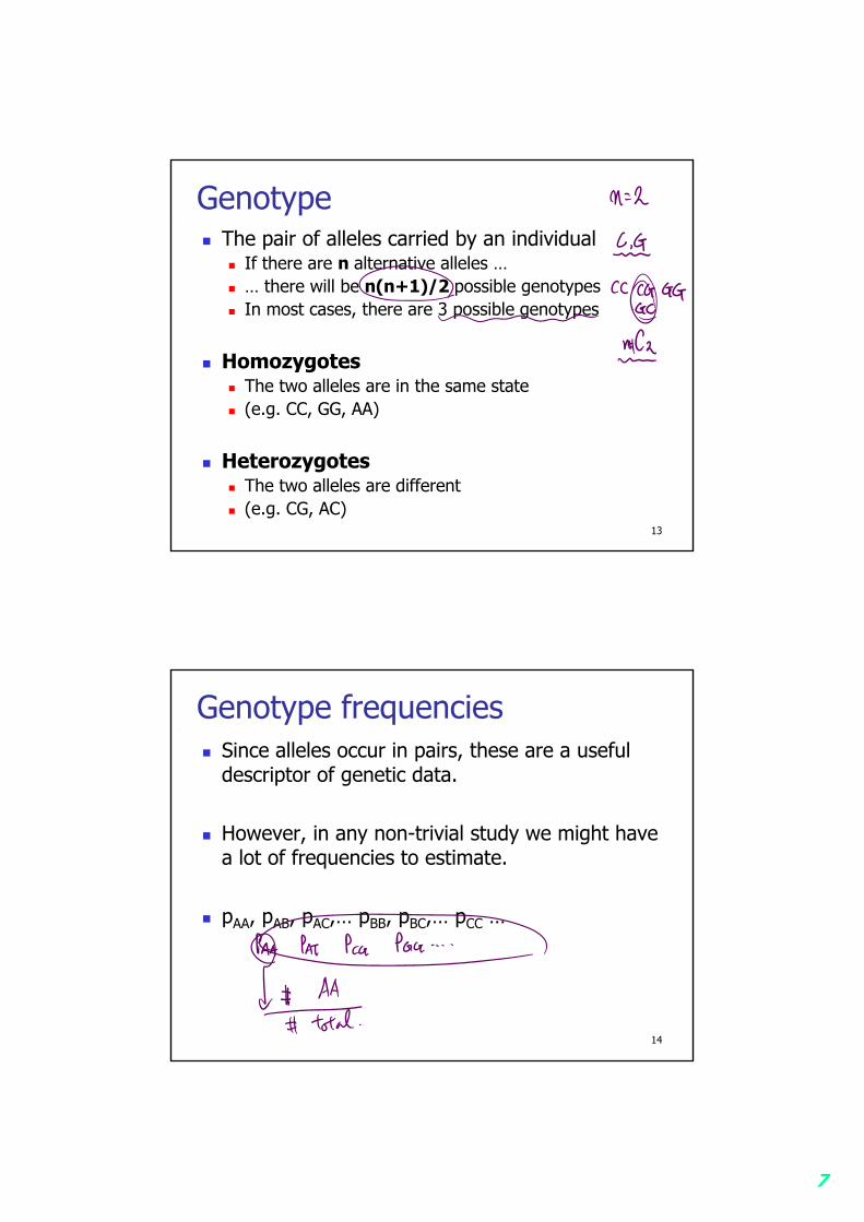
Genotype The pair of alleles carried by an individual

If there are n alternative alleles … … there will be n(n+1)/2 possible genotypes In most cases, there are 3 possible genotypes

Homozygotes The two alleles are in the same state (e.g. CC, GG, AA)

Heterozygotes The two alleles are different (e.g. CG, AC)

13

Genotype frequencies Since alleles occur in pairs, these are a useful

descriptor of genetic data.

However, in any non-trivial study we might have a lot of frequencies to estimate.

pAA, pAB, pAC,… pBB, pBC,… pCC …

14

8

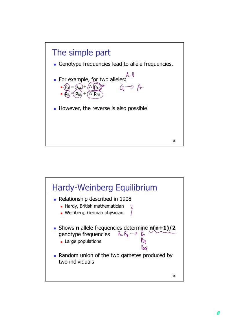
The simple part Genotype frequencies lead to allele frequencies.

For example, for two alleles: pA = pAA + ½ pAB

pB = pBB + ½ pAB

However, the reverse is also possible!

15

Hardy-Weinberg Equilibrium Relationship described in 1908

Hardy, British mathematician Weinberg, German physician

Shows n allele frequencies determine n(n+1)/2 genotype frequencies Large populations

Random union of the two gametes produced by two individuals

16

9

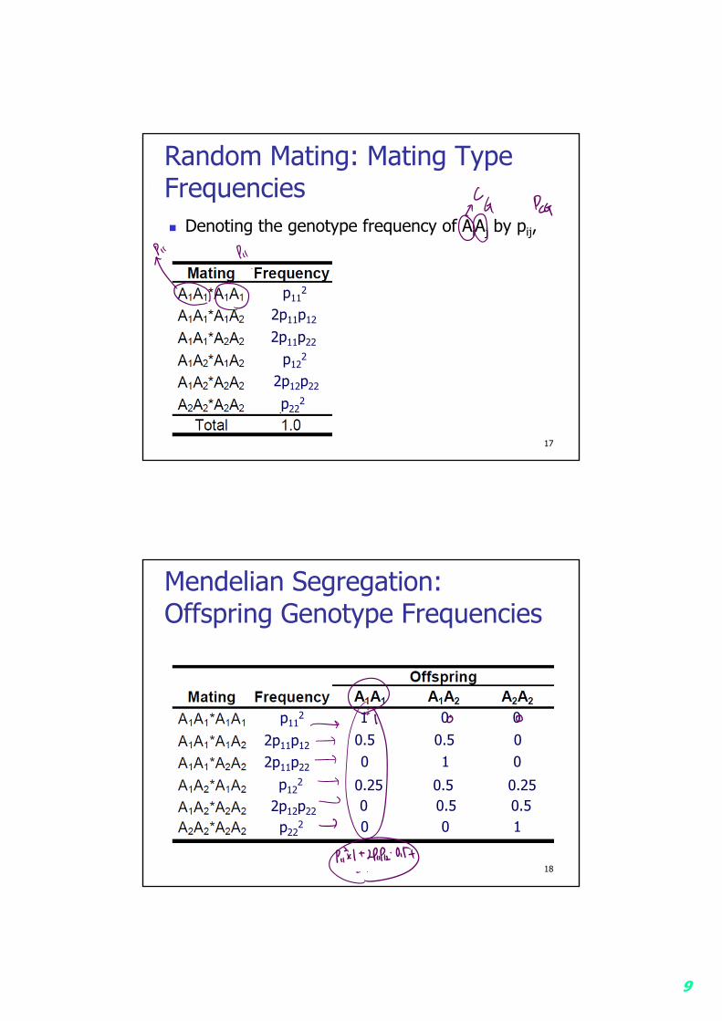
Random Mating: Mating Type Frequencies Denoting the genotype frequency of AiAj by pij,

17

p112

2p11p12

2p11p22

p122

2p12p22

p222

Mendelian Segregation: Offspring Genotype Frequencies

18

p112

2p11p12

2p11p22

p122

2p12p22

p222

1 0 00.5 0.5 00 1 0

0.25 0.5 0.250 0.5 0.50 0 1

10

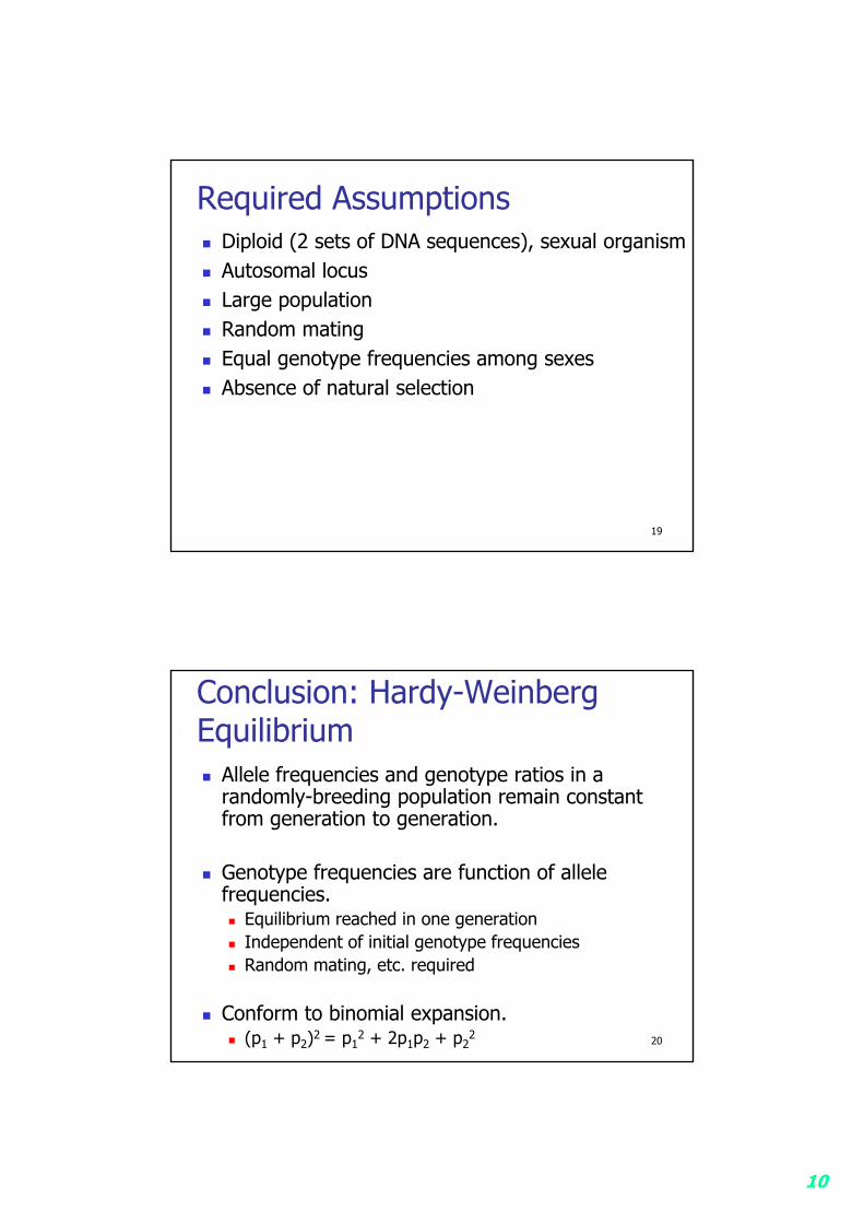
Required Assumptions Diploid (2 sets of DNA sequences), sexual organism Autosomal locus Large population Random mating Equal genotype frequencies among sexes Absence of natural selection

19

Conclusion: Hardy-Weinberg Equilibrium Allele frequencies and genotype ratios in a

randomly-breeding population remain constant from generation to generation.

Genotype frequencies are function of allele frequencies. Equilibrium reached in one generation Independent of initial genotype frequencies Random mating, etc. required

Conform to binomial expansion. (p1 + p2)2 = p1

2 + 2p1p2 + p22 20

11

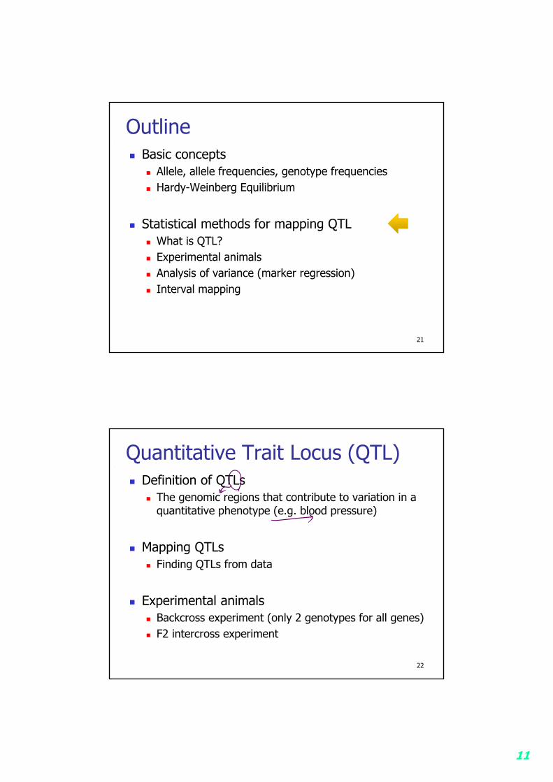
Outline Basic concepts

Allele, allele frequencies, genotype frequencies Hardy-Weinberg Equilibrium

Statistical methods for mapping QTL What is QTL? Experimental animals Analysis of variance (marker regression) Interval mapping

21

Quantitative Trait Locus (QTL) Definition of QTLs

The genomic regions that contribute to variation in a quantitative phenotype (e.g. blood pressure)

Mapping QTLs Finding QTLs from data

Experimental animals Backcross experiment (only 2 genotypes for all genes) F2 intercross experiment

22

12

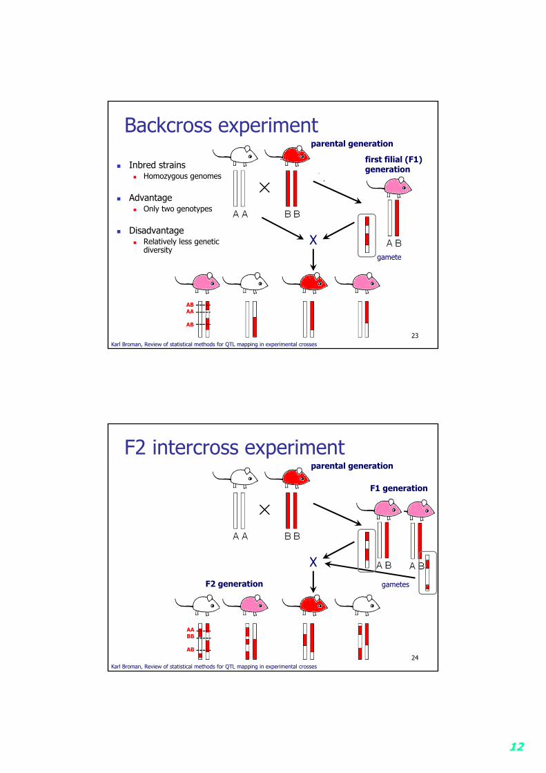
Backcross experiment

Inbred strains Homozygous genomes

Advantage Only two genotypes

Disadvantage Relatively less genetic

diversity

23Karl Broman, Review of statistical methods for QTL mapping in experimental crosses

first filial (F1) generation

parental generation

Xgamete

ABAA

AB

F2 intercross experiment

24Karl Broman, Review of statistical methods for QTL mapping in experimental crosses

F1 generation

parental generation

X

gametes F2 generation

AABB

AB

13

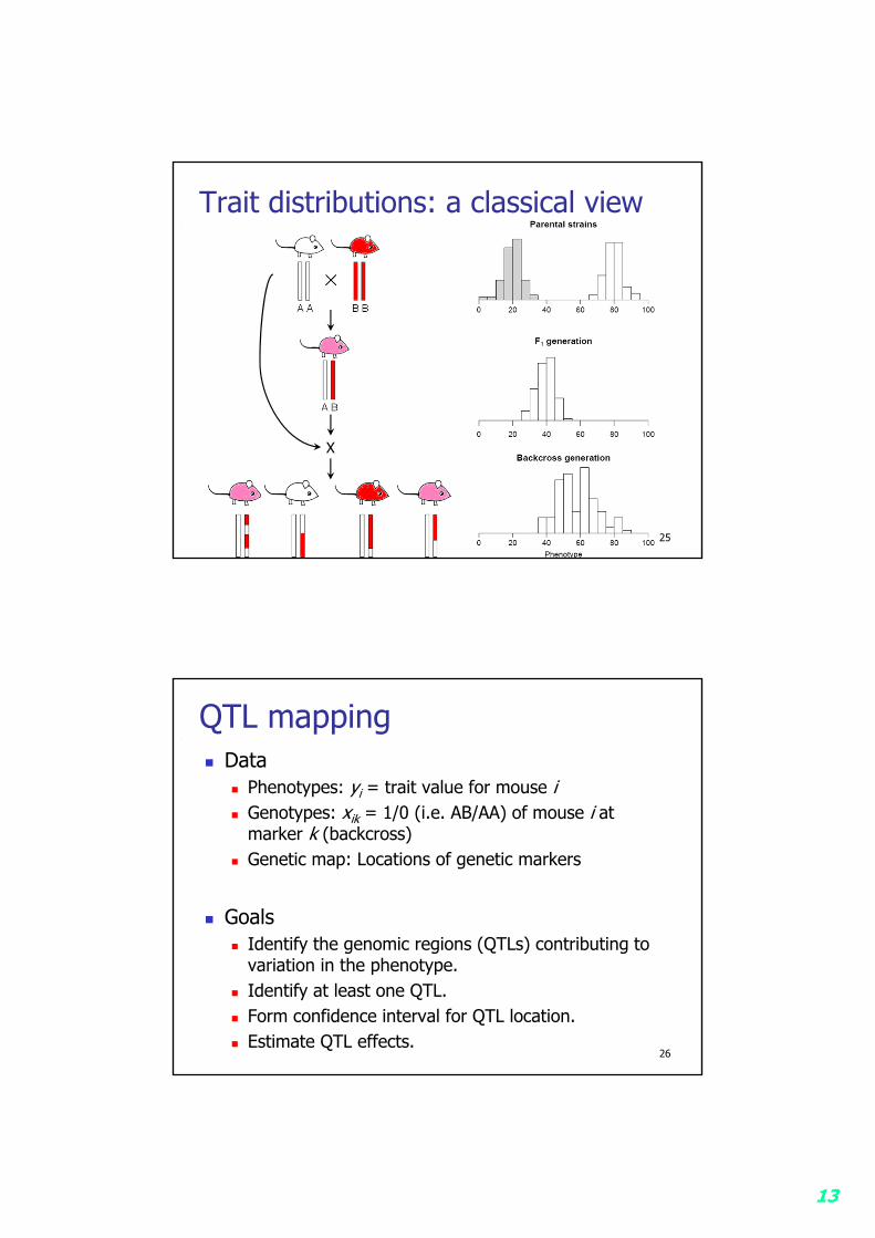
Trait distributions: a classical view

25

X

QTL mapping Data

Phenotypes: yi = trait value for mouse i Genotypes: xik = 1/0 (i.e. AB/AA) of mouse i at

marker k (backcross) Genetic map: Locations of genetic markers

Goals Identify the genomic regions (QTLs) contributing to

variation in the phenotype. Identify at least one QTL. Form confidence interval for QTL location. Estimate QTL effects.

26

14

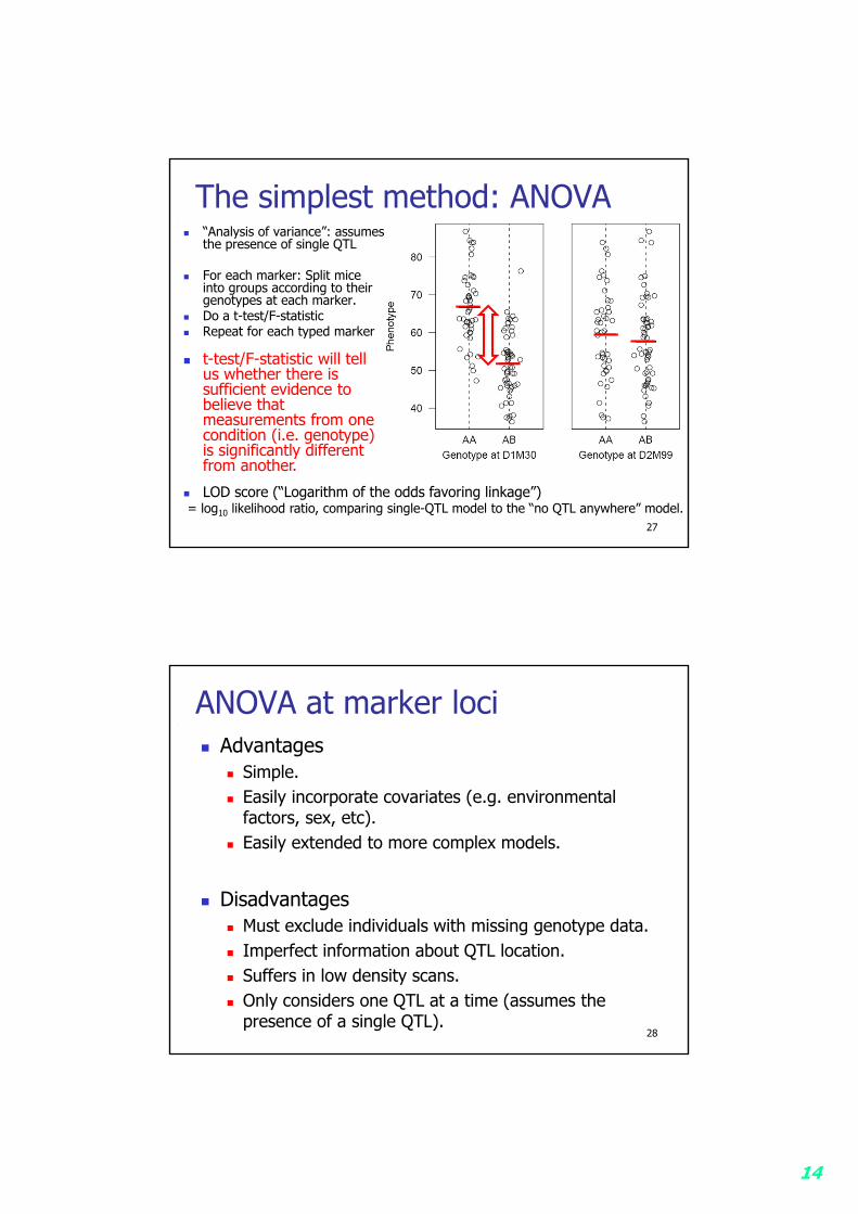
The simplest method: ANOVA

27

t-test/F-statistic will tell us whether there is sufficient evidence to believe that measurements from one condition (i.e. genotype) is significantly different from another.

LOD score (“Logarithm of the odds favoring linkage”)= log10 likelihood ratio, comparing single-QTL model to the “no QTL anywhere” model.

“Analysis of variance”: assumes the presence of single QTL

For each marker: Split mice into groups according to their genotypes at each marker.

Do a t-test/F-statistic Repeat for each typed marker

ANOVA at marker loci Advantages

Simple. Easily incorporate covariates (e.g. environmental

factors, sex, etc). Easily extended to more complex models.

Disadvantages Must exclude individuals with missing genotype data. Imperfect information about QTL location. Suffers in low density scans. Only considers one QTL at a time (assumes the

presence of a single QTL).28

15

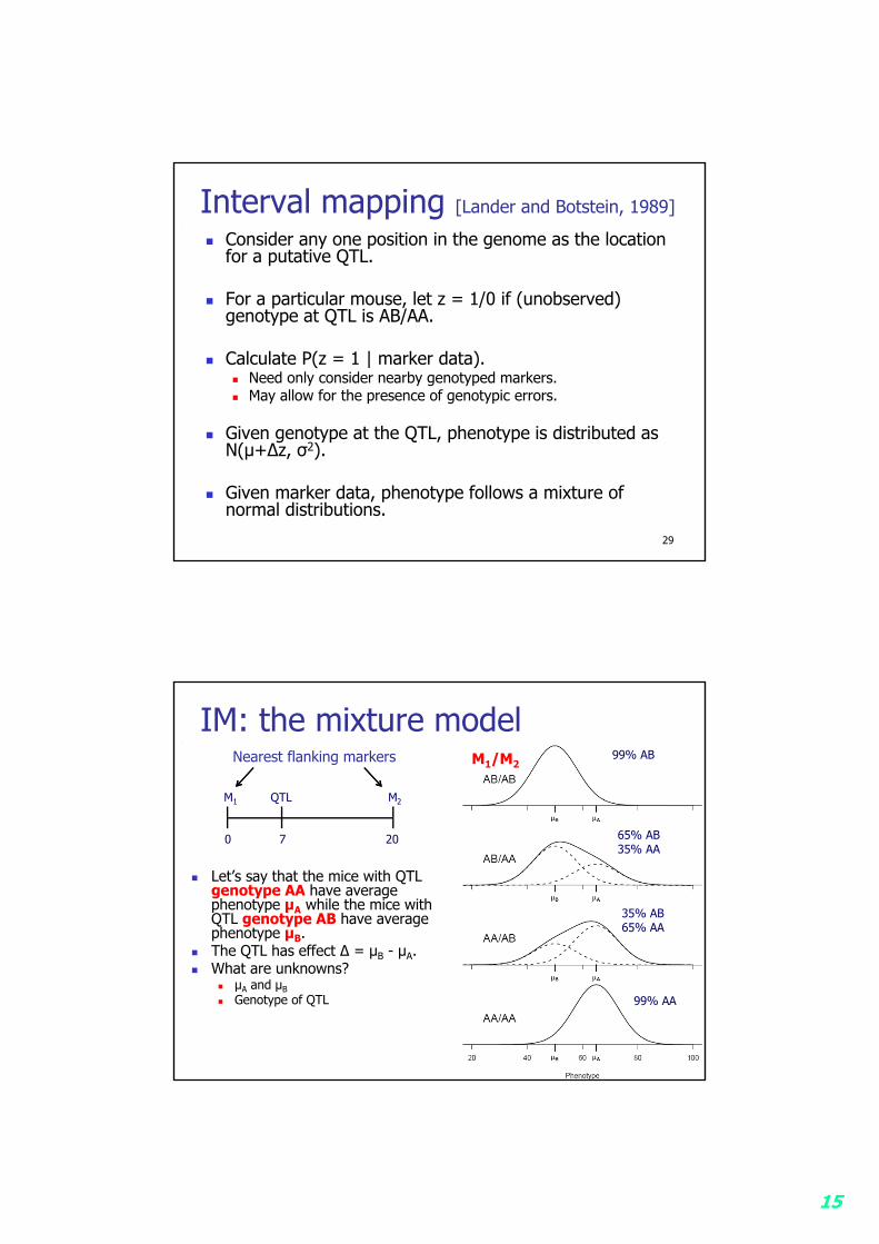
Interval mapping [Lander and Botstein, 1989]

Consider any one position in the genome as the location for a putative QTL.

For a particular mouse, let z = 1/0 if (unobserved) genotype at QTL is AB/AA.

Calculate P(z = 1 | marker data). Need only consider nearby genotyped markers. May allow for the presence of genotypic errors.

Given genotype at the QTL, phenotype is distributed as N(µ+∆z, σ2).

Given marker data, phenotype follows a mixture of normal distributions.

29

IM: the mixture model

Let’s say that the mice with QTL genotype AA have average phenotype µA while the mice with QTL genotype AB have average phenotype µB.

The QTL has effect ∆ = µB - µA. What are unknowns?

µA and µB Genotype of QTL

30

0 7 20

M1 QTL M2

M1/M2Nearest flanking markers

65% AB35% AA

35% AB65% AA

99% AB

99% AA

16

References Prof Goncalo Abecasis (Univ of Michigan)’s lecture note

Broman, K.W., Review of statistical methods for QTL mapping in experimental crosses

Doerge, R.W., et al. Statistical issues in the search for genes affecting quantitative traits in experimental populations. Stat. Sci.; 12:195-219, 1997.

Lynch, M. and Walsh, B. Genetics and analysis of quantitative traits. Sinauer Associates, Sunderland, MA, pp. 431-89, 1998.

Broman, K.W., Speed, T.P. A review of methods for identifying QTLs in experimental crosses, 1999.

31