Solution of Linear Programming

and Non-Linear Regression Problems

Using Linear M-Estimation Methods

Ove Edlund

Department of Mathematics,Lulea University of Technology,

S-971 87 Lulea, Sweden

July 1999

1

2

Abstract

This Ph.D. thesis is devoted to algorithms for two optimization problems, andtheir implementation. The algorithms are based on solving linear M-estimationproblems.

First, an algorithm for the non-linear M-estimation problem is considered.The main idea of the algorithm is to linearize the residual function in eachiteration and thus calculate the iteration step by solving a linear M-estimationproblem. A 2-norm bound on the variables restricts the step size, to guaranteeconvergence.

The other algorithm solves the linear programming problem. If a variablein the primal problem has both a lower and an upper bound, it gives rise toan edge in the dual objective function. This edge is “smoothed” by replacingit and its neighbourhood with a quadratic function, thus making it possible tosolve the approximated problem with Newton’s method. For variables with onlylower or only upper bounds, a quadratic penalty function is used on the dualproblem. In this way also variables with one-sided bounds can be handled. Acrucial property of the algorithm is that once the right active column set for theoptimal solution is identified, the optimal solution is found in one step.

The implementation uses sparse matrix techniques. Since it is an active setmethod, it is possible to reuse the old factor when calculating the new step.This is accomplished by up- and downdating the old factor, thus saving muchcomputation time. It is only occasionally, when the downdating fails, that thefactor instead has to be found with a sparse multifrontal LQ-factorization.

3

Acknowledgements

First of all, I would like to thank my supervisor, associate professor HakanEkblom. One way or another, he managed to get me a position as a Ph.D.student in numerical analysis at a time when the university did not recognizethis as a research area in its own right. Indeed, professor Lars-Erik Persson,Gerd Brandell and the department of mathematics also were very helpful in thisrespect. Things have improved since then, as the number of people involved inthis research area has grown. Also, the name of the research area has changedfrom numerical analysis to scientific computing.

During my studies, Hakan has always been very generous with his time,listening to whatever I had in mind, reading my manuscripts, and giving muchhelp in return.

I would also like to express my gratitude to professor Kaj Madsen and as-sociate professor Hans Bruun Nielsen at the department of mathematical mod-elling, DTU, Denmark. They have had a substantial input in all the articlesin the thesis and I have learned a lot by the discussions we have had. NordiskForskerutdanningsakademi (NorFA) has financially supported my visits to Den-mark, making this collaboration possible.

Finally, I would like to thank my wife, Susanne. The work on the thesishas taken more time than I anticipated, but still Susanne has put up with mylate nights and done more than her share of taking care of our children and thehousehold. Perhaps there will be a time when I can pay her back.

4

Contents

1 Introduction 7

2 Linear M-Estimation 8

3 Non-Linear M-Estimation 11

4 Using a Modified Huber-criterion for Solving Linear Program-ming Problems 12

5 The Concept of Sparse Matrices 14

Article I: Algorithms for Non-Linear M-Estimation 17

Article II: Linear M-Estimation with Bounded Variables 31

Article III: A Piecewise Quadratic Approach for Solving SparseLinear Programming Problems 51

Article IV: A Software Package for Sparse Orthogonal Factoriza-tion and Updating 79

5

6

1 Introduction

This Ph.D. thesis in scientific computing is devoted to the solution of two differ-ent optimization problems. The non-linear M-estimation problem comes fromthe field of robust regression. The objective is to identify parameters in a math-ematical model so that the model and real life observations match. The meaningof “robust” is that a few erroneous observations should not alter the solutionin a significant way. The other problem considered is the linear programmingproblem, that was formulated and solved by Danzig in the late 1940:s, and sincethen has found its use in many applications, including such different areas asintegrated circuit design, chemistry and economics.

Though these problems are very different, the two algorithms share the prop-erty that the solution is found by solving a sequence of linear M-estimationproblems.

Linear programming problems are frequently formulated with sparse ma-trices, and much computational work can be saved by taking the sparsity intoaccount. The linear programming algorithm has been implemented using sparsematrix techniques. The sparse matrix part of the implementation is the subjectof one of the articles in this thesis.

The thesis consists of four articles. The first two deal with solving thenon-linear M-estimation problem, and the following two describe the linear pro-gramming algorithm and implementation:

Article I: Edlund, O., Ekblom, H. & Madsen, K. (1997), ‘Algorithms for non-linear M-estimation’, Computational Statistics 12, 373–383.

Article II: Edlund, O. (1997), ‘Linear M-estimation with bounded variables’,BIT 37(1), 13–23.

Article III: Edlund, O., Madsen K. & Nielsen H. B. (1999), ‘A PiecewiseQuadratic Approach for Solving Sparse Linear Programming Problems’.To be submitted.

Article IV: Edlund, O. (1999), ‘A Software Package for Sparse OrthogonalFactorization and Updating’. To be submitted.

Beside these articles, the author has published two papers at conferences.One is a short note on solving linear Huber problems using a vector processor(Edlund 1994). The other paper is on algorithms for robust error-in-variablesproblems (Ekblom & Edlund 1998). This second paper describes a work inprogress. Unfortunately it did not evolve far enough to make it to the thesis.

The articles are preceded by a general introduction where the basic ideasof the algorithms are introduced. Section 2 describes briefly the concept oflinear M-estimation, the core in both of the algorithms. The case of nonlinearM-estimation is the subject of section 3. This serves as an introduction toArticle I–II. In section 4 the linear programming algorithm of Article III isintroduced. Section 5 gives a brief introduction to the area of sparse matrices,as a prelude to Article IV.

7

0 1 2 3 4 5 6 7 8

0

0.1

0.2

0.3

0.4

0.5

0.6

t

b

(t1, b

1)

(t2, b

2)

(t3, b

3)

(t4, b

4)

(t5, b

5)

(t6, b

6)

(t7, b

7)

(t8, b

8) (t

9, b

9)

Figure 1: The observations, and some randomly chosen model functions.

2 Linear M-Estimation

The M-estimates arise in robust statistics. Their purpose is to make a statisticalmodel that is not sensitive to gross errors in the data. The term “M-estimate” isto be interpreted as “maximum likelihood type estimate”, and is justified by thefact that the definition of an M-estimate is somewhat similar to the maximumlikelihood problem (Huber 1981).

To explain the principles of linear M-estimation, we will look at an example.Suppose that we have some observations (ti, bi) and there is a mathematicalmodel that describes the relation between t and b with the equation

b = x1 t+ x2 t e−t (1)

where x1 and x2 are unknown. In Figure 1 the observations are plotted, aswell as b as a function of t for some random [x1 x2]. The objective is to find avector [x1 x2] such that the equation is as close to the observations as possible.As seen in the figure, the observation (t7, b7) is very different compared to theothers and should be regarded as an erroneous observation.

We introduce a measurement of the distance from each observation to thefunction, called the residual as shown in Figure 2. The residual is a vectorcontaining as many elements as the number of observations. For our examplean element in the residual is defined as

ri = bi − x1 ti − x2 ti e−ti ,

8

0 1 2 3 4 5 6 7

0

0.1

0.2

0.3

0.4

0.5

0.6

t

b

r1

r2

r3

r4

r5

r6

r7

r8

r9

Figure 2: The elements of the residual.

thus the residual vector can be calculated as

r =

r1r2

...r9

=

b1b2...b9

−t1 t1e

−t1

t2 t2e−t2

......

t9 t9e−t9

︸ ︷︷ ︸

=A

[x1

x2

],

i.e. r = b−Ax where A is a constant matrix and b is a constant vector, and xis the unknown vector that is sought. The reason why we could formulate theresidual with the help of a matrix is that the elements of x are linear in (1). Themathematical model is often disregarded in the linear case, since it is sufficientto know the matrix A and the vector b to solve the problem. The more difficultnon-linear case is introduced in section 3 and is described in more detail inArticle I.

Looking at Figure 2, it is not difficult to imagine that the model equationis close to the observations if the elements of the residual are small, so ourobjective is to minimize the residual. This is done by constructing an objectivefunction that sums up the residual entries in a special way:

G(x) =m∑i=1

ρ(ri(x)).

Here ρ(t) is a positive function that is decreasing as t < 0 and increasing as t > 0.By finding the solution of minxG(x), the residual is minimized. This minimum

9

Table 1: ρ-functions for some M-estimates.

`1 estimateρ(t) = |t|

Huber estimate (k > 0)

ρ(t) =

�t2/2, |t| ≤ k

k|t| − k2/2, |t| > k

Fair estimate (k > 0)ρ(t) = k2(|t|/k − ln(1 + |t|/k))

Tukey estimate (k > 0)

ρ(t) =

�(k2/6)[1 − {1− (t/k)2}3], |t| ≤ k

k2/6, |t| > k

Welsh estimate (k > 0)

ρ(t) = k2/2�

1− e−(t/k)2�

varies though with the choice of ρ. The most common choice is ρ(t) = t2 whichgives the least squares solution. The least squares solution is easy to find bysolving the normal equations, though other methods have better stability froma numerical point of view. The least squares solution is the maximum likelihoodsolution if the errors are normally distributed, but it is not very good at handleerroneous observations, since there is a high penalty on large residual entriesdue to the square in the sum. Some robust choices of ρ, that are less sensitive toerroneous observations, are shown in Table 1. Solutions for different choices ofρ are called M-estimates. Many of the ρ-functions have a constant parameter k,so the solution found does not only vary with the choice of ρ, but also with thechoice of k.

Using some different ρ-functions to solve our example give the solutions inFigure 3. From the figure it is obvious that the Huber and Welsh estimates areless disturbed by the dissentient observation than the least squares estimate.

The choice of k should reflect a threshold between good residual elementsand bad ones corresponding to erroneous observations. To be able to do thischoice in a consistent way, the residual entries are often rescaled by a factor σ,giving the following problem

minimize G(x) =m∑i=1

ρ(ri(x)/σ). (2)

Finding the solution of (2) then comes in two flavours. Either the scale σis known, or it is not. In the second case σ can be found in the process ofsolving (2).

The fastest algorithms for solving linear M-estimation problems are based onNewton’s method with linesearch, though it demands that ρ(t) is continuouslydifferentiable. This rules out Newton’s method for finding `1 estimates. Otherpeculiar things happen if the ρ-functions are non-convex, as the case is for the

10

0 1 2 3 4 5 6 7

0

0.1

0.2

0.3

0.4

0.5

0.6

t

b

Least squaresHuberWelsh

Figure 3: Different M-estimates.

Tukey and Welsh estimates. Then the objective function G(x) may have manylocal minima. Newton’s method will find one of them, without any guaranteethat it is the global minimum.

Detailed information on different algorithms can be found in Dutter (1977),Huber (1981), O’Leary (1990), Antoch & Ekblom (1995), Ekblom & Nielsen(1996) and Article II in this thesis. The important case of finding linear Huberestimates is covered in e.g. Clark & Osborne (1986), Ekblom (1988) and Madsen& Nielsen (1990).

3 Non-Linear M-Estimation

In non-linear M-estimation, the residual is a vector valued function f : Rn −→Rm with m > n. The non-linear M-estimator is defined as the x ∈ Rn thatsolves

minimizem∑i=1

ρ(fi(x)/σ). (3)

As before, σ is the scale of the problem. In the non-linear case it is no longerguaranteed that we have a convex optimization problem, even if ρ(t) is convex.Finding the global minimum of a problem with possibly many local minima isstill an unsolved problem. Therefore, algorithms for this kind of optimizationproblems (also in the non-linear least squares case) only find a local minimum.

The problem of finding non-linear M-estimators have been treated e.g. inDennis (1977), Dutter & Huber (1981), Gay & Welsch (1988) and Ekblom &

11

Madsen (1989). The approach taken here is the one used in Ekblom & Madsen(1989), but with general M-estimation, instead of only Huber estimation, andwith a new approach to solve the local problem.

The basic ideas behind Article I are the following: The scale parameter σis supposed to be a known constant. A local minimum to (3) is found with aniterative process. At iteration k we make a linearization of f(x) at xk,

l(h) = f (xk) + J(xk)h

where J(xk) is the Jacobian matrix of f(x) at xk. Then we solve

minimizem∑i=1

ρ(li(h)/σ),

subject to ‖h‖2 ≤ δ.(4)

This is a linear M-estimation problem. The difference from (2) is that there is abound on the variables, since we only can trust the linear approximation of f(x)in a neighbourhood of xk, i.e. this is a trust region approach. Let the solutionof (4) be hk, then the next step in the iteration is given by xk+1 = xk + hk.

Finding solutions to (4) is the subject of Article II and solving (3) is thesubject of Article I of this thesis. Note that the appendix of Article II is notpresent in the published paper (Edlund 1997).

4 Using a Modified Huber-criterion for Solving

Linear Programming Problems

This section will focus on the correspondence between linear programming prob-lems and M-estimation problems. Luenberger (1984) has information on prop-erties of linear programming problems and how they are modelled.

The background to all this is that there is a duality correspondence betweenthe linear `1 problem and a linear programming problem. As mentioned insection 2 Newton’s method with linesearch does not work for the `1 problem.The reason is that there is an edge in the objective function at the solution,and thus methods that seek zero gradients will fail. Ekblom (1987) proposedthat the linear `1 estimate could be found by a series of linear Huber estimates.Using the Huber ρ-function

ρ(γ)(t) ={ 1

2γ t2, |t| ≤ γ

|t| − γ2 , |t| > γ

, (5)

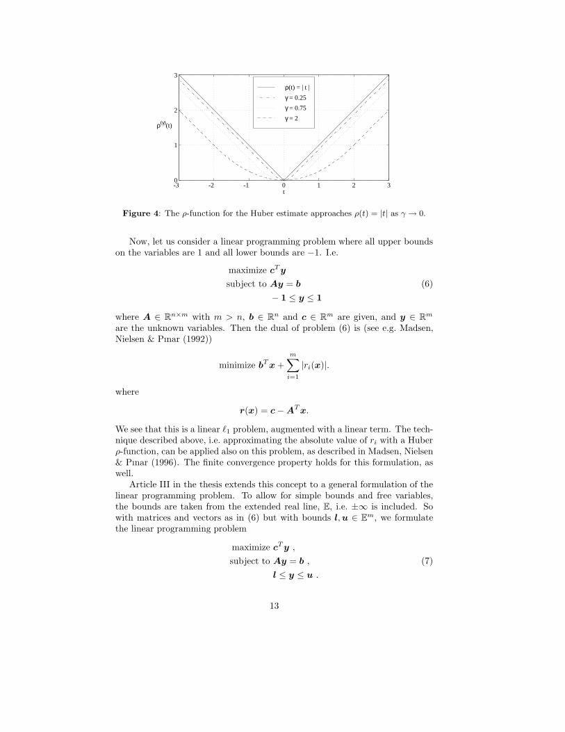
we see (Figure 4) that this function approaches ρ(t) = |t| as γ → 0, giving the`1 estimate in the limit.

Madsen & Nielsen (1993) showed that there exists a threshold γ0 such thatthe `1 solution can be found immediately whenever γ ≤ γ0. Using this fact andtheir finite algorithm for finding Huber estimates (Madsen & Nielsen 1990) theygot a finite algorithm for finding `1 estimates.

12

-3 -2 -1 0 1 2 30

1

2

3

t

ρ(γ)(t)

ρ(t) = | t |

γ = 0.25

γ = 0.75

γ = 2

Figure 4: The ρ-function for the Huber estimate approaches ρ(t) = |t| as γ → 0.

Now, let us consider a linear programming problem where all upper boundson the variables are 1 and all lower bounds are −1. I.e.

maximize cTysubject to Ay = b

− 1 ≤ y ≤ 1

(6)

where A ∈ Rn×m with m > n, b ∈ Rn and c ∈ Rm are given, and y ∈ Rmare the unknown variables. Then the dual of problem (6) is (see e.g. Madsen,Nielsen & Pınar (1992))

minimize bTx+m∑i=1

|ri(x)|.

where

r(x) = c−ATx.

We see that this is a linear `1 problem, augmented with a linear term. The tech-nique described above, i.e. approximating the absolute value of ri with a Huberρ-function, can be applied also on this problem, as described in Madsen, Nielsen& Pınar (1996). The finite convergence property holds for this formulation, aswell.

Article III in the thesis extends this concept to a general formulation of thelinear programming problem. To allow for simple bounds and free variables,the bounds are taken from the extended real line, E, i.e. ±∞ is included. Sowith matrices and vectors as in (6) but with bounds l,u ∈ Em, we formulatethe linear programming problem

maximize cTy ,subject to Ay = b ,

l ≤ y ≤ u .

(7)

13

The approximation of the dual of (7) then looks like this:

minimize Gγ(x) = bTx+m∑i=1

ρ(γ)i (ri(x))

where r(x) = c−ATx and

ρ(γ)i (t) =

lit− γ

2 l2i , t < γli

12γ t

2, γli ≤ t ≤ γuiuit− γ

2u2i , t > γui

.

Article III shows the relevance of this. Note that there are different ρ-functionsfor each residual element. The ρ-functions are really just variations of the Huberρ-function, which is obvious by inserting li = −1 and ui = 1 and comparing with(5). For infinite bounds, the corresponding ρ-function is a penalty function,that ensures that the inequality constraint of the dual is fulfilled as γ → 0.Furthermore, the same properties hold as before.

5 The Concept of Sparse Matrices

A matrix should be considered sparse if it mostly consists of zeros. Since thesezeros make no contribution to the matrix calculations, computation time andcomputer memory can be saved. This is accomplished by using sparse matrixstorage schemes, where only the non-zero entries and their positions are stored.Note that any matrix can be expressed with sparse storage schemes as well aswith a dense scheme. However, for every matrix one of the schemes is moreefficient. This suggests that a matrix should be considered sparse, if the calcu-lations involving the matrix are executed more efficiently using a sparse storagescheme than using a dense one. From a strictly mathematical point of view, thenotion of sparse matrices is uninteresting, since there is no separate theoreticaltreatment for sparse matrices.

As an example of a sparse matrix, Figure 5 shows the positions for the non-zeros of the matrix A from the linear programming test problem “25fv47”. Indifferent areas, systems involving sparse matrices are solved in different ways.In the area of partial differential equations, iterative methods are often used,while linear programming solvers most often use direct methods. The sparsematrix software package spLQ described in Article IV uses direct methods tofactorize the matrix before the system is solved. The subject of direct methodsfor sparse systems is treated in Duff, Erisman & Reid (1986), as well as differentsparse storage schemes, while the specific method used in Article IV is describedin Matstoms (1994).

14

0 200 400 600 800 1000 1200 1400 1600 1800

0

100

200

300

400

500

600

700

800

nz = 10705

Figure 5: Non-zero structure for the constraint matrix A of the linear programming

test problem “25fv47”.

References

Antoch, J. & Ekblom, H. (1995), ‘Recursive robust regression. Computa-tional aspects and comparison’, Computational Statistics and Data Analy-sis 19, 115–128.

Clark, D. I. & Osborne, M. R. (1986), ‘Finite algorithms for Huber’s M-estimator’, SIAM J. Sci. Statist. Comput. 7, 72–85.

Dennis, Jnr., J. E. (1977), Non-linear least squares and equations, in D. A. H.Jacobs, ed., ‘State of the Art in Numerical Analysis’, Academic Press,pp. 269–213.

Duff, I. S., Erisman, A. M. & Reid, J. K. (1986), Direct Methods for SparseMatrices, Oxford University Press.

Dutter, R. (1977), ‘Numerical solution of robust regression problems: Compu-tational aspects, a comparison’, J. Statist. Comput. Simul. 5, 207–238.

Dutter, R. & Huber, P. J. (1981), ‘Numerical methods for the nonlinear robustregression problem’, J. Statist. Comput. Simul .

Edlund, O. (1994), A study of possible speed-up when using a vector processor,in R. Dutter & W. Grossman, eds, ‘Short Communications in Computa-tional Statistics’, COMPSTAT 94, pp. 2–3.

Edlund, O. (1997), ‘Linear M-estimation with bounded variables’, BIT37(1), 13–23.

Ekblom, H. (1987), The L1-estimate as limiting case of an Lp- or Huber-estimate, in Y. Dodge, ed., ‘Statistical Analysis Based on the L1-Normand Related Methods’, Elsevier Science Publishers, pp. 109–116.

15

Ekblom, H. (1988), ‘A new algorithm for the Huber estimator in linear models’,BIT 28, 123–132.

Ekblom, H. & Edlund, O. (1998), Algorithms for robustified error-in-variablesproblems, in R. Payne & P. Green, eds, ‘Proceedings in ComputationalStatistics’, COMPSTAT 1998, Physica-Verlag, Heidelberg, pp. 293–298.

Ekblom, H. & Madsen, K. (1989), ‘Algorithms for non-linear Huber estimation’,BIT 29, 60–76.

Ekblom, H. & Nielsen, H. B. (1996), A comparison of eight algorithms forcomputing M-estimates, Technical Report IMM-REP-1996-15, Institute ofMathematical Modelling, Technical University of Denmark, Lyngby 2800,Denmark.

Gay, D. & Welsch, R. (1988), ‘Nonlinear exponential family regression models’,JASA 83, 990–998.

Huber, P. (1981), Robust Statistics, John Wiley, New York.

Luenberger, D. (1984), Linear and Nonlinear Programming, Addison-Wesley.

Madsen, K. & Nielsen, H. B. (1990), ‘Finite algorithms for robust linear regres-sion’, BIT 30, 333–356.

Madsen, K. & Nielsen, H. B. (1993), ‘A finite smoothing algorithm for linear `1estimation’, SIAM J. Optimization 3(2), 223–235.

Madsen, K., Nielsen, H. B. & Pınar, M. C. (1992), Linear, quadratic and min-imax programming using l1 optimization, Technical Report NI-92-11, In-stitute for Numerical Analysis, Technical University of Denmark, Lyngby2800, Denmark.

Madsen, K., Nielsen, H. B. & Pınar, M. C. (1996), ‘A new finite continuationalgorithm for linear programming’, SIAM J. Optimization 6(3), 600–616.

Matstoms, P. (1994), Sparse QR Factorization with Applications to LinearLeast Squares Problems, Ph.D. dissertation, Department of Mathematics,Linkoping University, S-581 83 Linkoping, Sweden.

O’Leary, D. P. (1990), ‘Robust regression computation using iterativelyreweighted least squares’, SIAM J. Matrix Anal. Appl. 11, 466–480.

16

Article I

Algorithms for Non-Linear

M-Estimation

Published in Computational Statistics 12, 1997, pp. 373–383.

17

18

Algorithms for Non-Linear M-Estimation

Ove Edlund1, Hakan Ekblom1 and Kaj Madsen2

1Department of Mathematics, Lulea University of Technology,S-97187 Lulea, Sweden

2Institute of Mathematical Modelling, Technical University of Denmark,DK-2800 Lyngby, Denmark

Abstract

In non-linear regression, the least squares method is most often used.Since this estimator is highly sensitive to outliers in the data, alternativeshave become increasingly popular during the last decades. We presentalgorithms for non-linear M-estimation. A trust region approach is used,where a sequence of estimation problems for linearized models is solved.In the testing we apply four estimators to ten non-linear data fitting prob-lems. The test problems are also solved by the Generalized Levenberg-Marquardt method and standard optimization BFGS method. It turnsout that the new method is in general more reliable and efficient.

1 Introduction

A very common problem in engineering, science and economy is to fit a givenmathematical model to a set of data. The model depends on a number ofparameters which must be determined. For this fitting problem the least squarescriterion has been intensively used for about two centuries. Using this criterionthe data fitting problem can be formulated as follows:

Minimizem∑i=1

ρ(fi(x)) (1)

where ρ(t) = t2/2,fj : Rn −→ R, (j = 1, . . . ,m) is a setof non-linear functions,x is an n-vector of “parameters”.

Here the function values fj are residuals when fitting a model function g(t,x)to a set of points (tj , yj), j = 1, . . . ,m, i.e. we have

fj(x) = yj − g(tj ,x), j = 1, . . . ,m. (2)

19

The last three decades have seen an increasing interest in replacing the leastsquares method by more “robust” criteria, i.e. estimators more resistant tocontaminated data. One possibility is to choose ρ in a different way, whichgives so called M-estimates (Huber 1981).

It is necessary to make the residuals scale invariant in order to make therobust criteria work. We therefore introduce a scale parameter σ and minimize

F (x) =m∑i=1

ρ(fi(x)/σ). (3)

The scale σ may be known in advance or it may have to be estimated from thedata. Here we assume its value to be fixed.

Some suggested alternatives to least squares are listed below (Huber 1981,Hampel et al. 1986, Gonin & Money 1989, Antoch & Visek 1992)

Lp estimate (1 ≤ p < 2)ρ(t) = |t|p

Huber estimate (b > 0)

ρ(t) ={

t2/2, |t| ≤ bb|t| − b2/2, |t| > b

Fair estimate (c > 0)ρ(t) = c2(|t|/c− ln(1 + |t|/c))

Welsh estimate (d > 0)ρ(t) = d2/2(1− e−(t/d)2

)

It should be noted that the last three alternatives give the least squaresestimate as limiting case when the tuning parameter approaches infinity. Fur-thermore, if we let b and c tend to zero the Huber and Fair estimates willapproach the L1-estimate, i.e. the least absolute deviations estimate. The val-ues of p, b, c, and d should be chosen to reflect the ratio of “bad values” in data(Ekblom & Madsen 1989, Huber 1981).

Example In Bates & Watts (1988) a data set (A4.5) is given which describesthe growth of leaves. The model function

g(t,x) =x1

(1 + x2e−x3t)1/x4

is to be fitted to 15 data points (tj , yj), j = 1, . . . , 15, where tj = j − 0.5 andy = (1.3, 1.3, 1.9, 3.4, 5.3, 7.1, 10.6, 16.0, 16.4, 18.3, 20.9, 20.5, 21.3, 21.2,20.9). Now assume that the leaf length entry no. 13 (21.3) is wrongly recordedas 5.0. The resulting fit for some different criteria is given in figure 1. It is seenthat the least squares estimate is much more affected by the outliers than thealternatives.

A look at ρ′(t) for the four alternatives above reveals their different behaviour(figure 2). One way to characterize an estimate is through its so-called influence

20

0 5 10 150

5

10

15

20

25

time

leng

th

Figure 1: The solid line is the L2 estimate, the dotted line is the Lp estimate, the

dashed line is the Huber estimate and the dash-dotted line is the Welsh estimate.

The Fair estimate is very similar to the Huber estimate in this problem. The tuning

parameters were chosen as p = b = c = d = 1.5.

-4 -3 -2 -1 0 1 2 3 4-3

-2

-1

0

1

2

3

t

Least Squares

Lp, p=1.5

Huber, b=1.5

Fair, c=1.5

Welsh, d=1.5

Figure 2: Some different ρ′(t).

21

function, which is proportional to ρ′(t) for these M-estimators (Hampel et al.1986). In short, the influence function shows how strongly a new observationcan affect the old estimate. Thus, to handle arbitrarily large errors in dataproperly, ρ′(t) should be limited. Figure 2 indicates that this is not the case forLp-estimates if p > 1. On the other hand, Lp-estimates have an advantage inbeing independent of the scaling parameter σ.

The Welsh estimate is of a special character since ρ′(t) approaches zerowhen |t| → ∞ . This corresponds to rejecting strongly deviating observations.However, this also means that the objective function is not necessarily convexeven for linear models, and hence there may be many local minima present.From algorithmic point of view, which is our main concern in this paper, thisis a highly undesirable situation. This is the reason why estimation based onthe Welsh function and other similar criteria are not included in this study.On the other hand, with a good starting point, there is a good chance to findthe solution also with non-convex criteria. One possibility is to use the Hubersolution as starting point. In case the true solution is found for e.g. the Welshcriterion, we can expect about the same algorithmic efficiency as for the Huberand Fair criteria, since the Welsh, Huber and Fair functions are very similarclose to the origin.

In this paper we focus on the non-linear version of the M-estimation problem.We will require fj to be at least twice differentiable and ρ to have a continuousderivative.

2 A new algorithm

Algorithms for non-linear robust estimation are often inspired by non-linearleast squares algorithms. As an example, the algorithm given by Dennis (1977)is a generalization of the Levenberg-Marquardt algorithm. Gay & Welsch (1988)use secant update to estimate the “messy” part of the Hessian (the differencebetween applying the Newton and Gauss-Newton methods). However, Gay &Welsch (1988) assume that the ρ function is twice differentiable, which is neitherthe case for Lp-estimation when p < 2 nor the Huber estimate.

The new method we propose in this paper for solving (3) is of the trust regiontype (More 1983). Such methods are iterative. Versions of the new algorithm forthe Huber criterion are found in Ekblom & Madsen (1989) and forLp estimationin Ekblom & Madsen (1992). At each iterate xk a local model, qk say, of theobjective function F is used. This local model should be “simpler” than thenon-linear objective, and it should reflect the characteristics of the objective. Inorder to find the next iterate, qk is minimized subject to the constraint that thesolution should be within a specified neighbourhood Nk of xk. Nk is intendedto reflect the domain in which the local model is a good approximation to thenon-linear objective. The size of the trust region is updated automatically aftereach iteration.

The local models we apply are based on linearizing the functions fj definingF . At each iterate xk the linear approximations lj(h;xk) = fj(xk) +f ′j(xk)Th

22

to fj , j = 1, . . . ,m are inserted in (3) instead of fj.Thus the local model at xk is defined as follows:

qk(h) ≡ q(h;xk) =m∑j=1

ρ(lj(h;xk)/σ) (4)

As the trust region at xk we use

Nk ≡ {y | y = xk + h, ‖h‖ ≤ δk} (5)

where δk > 0 is given and should reflect the amount of linearity of fj , j =1, . . . ,m, near xk.

Now the minimizer of (4) subject to (5) can be found by the method inEdlund (1997). A short description of this method is found in appendix. Theminimizer is denoted by hk and the new iterate is xk+hk. It is accepted if thereis a decrease in the objective function F which exceeds a small multiple of thedecrease predicted by the local model. Otherwise the trust region is diminishedand another iteration is performed from xk.

The trust region radius δk is updated according to the usual updating pro-cedures (see for instance More (1983)). It is based on the ratio between thedecrease in the non-linear function (which may be negative!) and the decreasein the local model (which is necessarily non-negative).

rk = max(0, [F (xk)− F (xk + hk)]/[qk(0)− qk(hk)])

More precisely, the trust region algorithm is the following:

Trust region algorithm:Let 0 < s1 � 0.25 and 0.25 ≤ s2 < 1 < s3.given x0 and δ0; k := 0;while not OUTERSTOP do begin

find the minimum hk of (4) subject to (5) ;if rk > s1 then xk+1 := xk + hk

else xk+1 := xk;if rk < 0.25 then δk+1 := δk · s2

else if rk > 0.75 then δk+1 := δk · s3

else δk+1 := δk;k := k + 1

end

OUTERSTOP could be the condition that

‖F ′(xk)‖ < ε1 or ‖hk‖ < ε2 ‖xk‖ ,

where ε1 and ε2 are suitably chosen tolerance parameters.As is usual for trust region methods this method is not sensitive to the choice

of the constants s1, s2 and s3. In our testing below we have used s1 = 0.001,s2 = 0.25 and s3 = 2.

23

Since the algorithm follows the general structure given in Madsen (1985)the usual convergence theory for trust region methods (More 1983) holds. Thismeans that under mild conditions convergence to the set of stationary points ofF is guaranteed.

3 Numerical experiments

3.1 Experimental design and results

The tests were carried out on 10 problems. The first five (further describedin More et al. (1981)) are standard numerical problems. In the last five (fromBates & Watts (1988)) the model function is fitted to real data.

Prob n m Name Model function1 5 33 Osborne x1 + x2e

−tx4 + x3e−tx5

2 3 15 Bard x1+t/[x2(16−t)+x3min(t, 16−t)]3 4 11 Kowalik-Osborne x1(t2 + tx2)/(t2 + tx3 + x4)4 3 16 Meyer x1e

x2/(t+x3)

5 4 20 Brown-Dennis (x1+tix2−eti)2+(x3+sin(ti)x4−cos(ti))2

6 3 54 Chloride x1(1− x2e−x3t)

7 4 15 Leaves x1/(1 + x2e−x3t)1/x4

8 9 53 Lubricant x1/(x2 + t1)+x3t2 +x4t22 +x5t

32 +

(x6 + x7t22)e−t1/(x8+x9t

22)

9 3 8 Nitrite(1st day) x1t/(x2 + t+ x3t2)

10 4 9 Saccharin (x3/x1)e−x1t1(1 − e−x1t2) +(x4/x2)e−x2t1(1− e−x2t2)

Three methods were used in the test:

Method 1: The method proposed in this paper, implemented along the linesgiven in Edlund (1997) and shortly outlined in appendix.

Method 2: The “Generalized Levenberg-Marquardt Algorithm” (Dennis1977).

Method 3: The BFGS-algorithm, a standard general optimization method(Fletcher 1987).

Tables 1–3 give the number of function evaluations of F (x) when the threemethods were applied to the ten problems for the three convex object functions.

3.2 Discussion of test results

Method 2 uses a general quadratic model of the objective function and thus doesnot exploit the supplementary information present in the problem correspondingto the linearized local model. In contrast, Method 1 keeps the structure of thenon-linear problem for the linearized models. Thus it is not surprising that

24

Table 1: Test results with Lp-estimation

Problem 1 2 3 4 5 6 7 8 9 10

p = 2 Method 1 19 7 34 129 38 19 46 9 18 14Method 2 19 7 34 129 310a 19 46 9 18 14Method 3 88 21 28 – 34 39 84 – 38b 66

p = 1.75 Method 1 21 7 33 162b 151 19 43 9 18 14

Method 2 18 11 34 133 40 19 43 94b 21 35

Method 3 89 32 27 – 27 42 92 – 46b 57

p = 1.5 Method 1 27 8 24 110 54 19 43 8 18 13Method 2 44 54 48 161 43 23 44 108b 53 63

Method 3 97 36 38 – 35 45 105 – 32b 71

p = 1.25 Method 1 41 8 23 107 94 20 38 9 16 15Method 2 248 111 72 – 65 87 108 343a 36b 189

Method 3 144 39 48 – 33 79 125 – 37b 139a Maximum number of iterationsb Inaccurate result‘–’ Completely wrong or no result

Table 2: Test results with Huber-estimationProblem 1 2 3 4 5 6 7 8 9 10

h = 2 Method 1 25 7 35 122 83 17 38 8 18 15Method 2 52 17 43 – 311a 22 46 – 52 –

Method 3 95 21 31 – 29 52 106 – 35b 63

h = 1.5 Method 1 21 7 22 124 308a 15 38 8 18 18Method 2 43 17 34 – 309a 22 – – 50 –Method 3 93 21 32 – 19 42 109 – 40b 66

h = 1 Method 1 31 7 15 279 308a 19 41 8 18 15Method 2 80 16 23 – 311a 28 – – 53 –

Method 3 92 19 35 – 37 41 114 – 38b 66

h = 0.5 Method 1 21 8 13 263 302a 22 41 9 18 13Method 2 131 25 22 – 303a 23 – – 55 –

Method 3 101 20 30 – 23 44 106 – 35b 102a Maximum number of iterationsb Inaccurate result‘–’ Completely wrong or no result

25

Table 3: Test results with Fair-estimationProblem 1 2 3 4 5 6 7 8 9 10

c = 3 Method 1 24 7 31 136 310a 17 43 8 18 13Method 2 40 15 43 322 308a 25 43 – 49 19Method 3 83 19 32 – 21 50 98 – 33b 76

c = 2 Method 1 22 7 29 135 215 17 42 8 19 14Method 2 41 17 36 338 310a 22 43 – 52 39

Method 3 92 26 32 – 21 44 112 – 31b 58

c = 1 Method 1 22 8 28 123 307a 19 43 8 20 14Method 2 48 19 36 – 309a 24 45 – 53 45Method 3 98 20 29 – 21 49 105 – 103 69

a Maximum number of iterationsb Inaccurate result‘–’ Completely wrong or no result

Method 2 needs more function evaluations, and often many more. Also in somecases, it fails to find the solution.

Method 3 uses about the same number of function evaluations as Method 1in some cases, but usually it requires at least twice as many. It may also giveinaccurate or totally wrong results in some cases. The Brown-Dennis problem(no. 5) shows a different picture. It is a so-called large residual problem, wherethe model function gives a very poor fit to the data. It is well known thatmethods related to Gauss-Newton methods (e.g. Method 1 and 2) perform badlyfor such problems, since the approximation to the Hessian comes to be veryinaccurate.

Finally we should mention that we have also done testing with some outliersintroduced to the test problems. This gave the same overall picture as in thetables presented, but with Method 1 even more in favour.

4 Conclusions

We propose a new iterative method of the trust region type. At each iterate thenon-linear model is linearized so that the non-linear functions fi are replacedby linear local approximations.

There are two kinds of non-linearities involved in the problem we are solv-ing, namely those present in the model function and those stemming from thecriterion used. The main idea of the algorithms we propose is to separate theseso that a sequence of linear robust estimation problems are solved during theiterations. The effect of this approach is seen in the test results, where the num-ber of function evaluations is very little influenced by the choice of parametervalue (“tuning constant”) in the ρ functions.

The algorithm proposed by Dennis (Method 2 in the testing) correspondsto making only one iteration when solving the linearized robust model, and canbe regarded as a much simplified version of the type method we propose. If astandard optimization code is used, like the BFGS method, the special character

26

of the data fitting problem is not taken into account. Although the result withsuch a method in some cases can be quite good, the test results shows that thereis a clear risk of inefficiency or inaccuracy.

Appendix:Finding the Minimum of the Local Model

A thorough description of a method to find minima of the linearized model witha 2-norm bound on the variables can be found in Edlund (1997). What followsis a rough description of the same method.

When qk(h) is minimized subject to ‖h‖ ≤ δ, the constraint is active only ifthe minimum of qk(h) is outside the trust region. In that case the solution canbe found by minimizing the Lagrangian function

sk(h) = qk(h) + λ(‖h‖2 − δ2k),

for a sequence of different values of the Lagrange-multiplier λ. Here ‖·‖ denotesthe 2-norm. Let h(λ) denote the minimizer of sk(h) for a certain λ. Then ateach minimizer h(λ), the Lagrange-multiplier λ is updated with the Hebden-iteration

λ := λ+(

1− ‖h(λ)‖δ

)‖h(λ)‖ddλ‖h(λ)‖

, (6)

until | ‖h(λ)‖ − δk| ≤ 0.1δk. In this way a sufficiently accurate approximationof λ is found, and we let hk = h(λ).

This algorithm will not work properly unless some mechanism for detectingwhen the constraint is not active (i.e. ‖hk‖ < δk) is included. Furthermore,some restrictions on the updating of λ is required to guarantee convergence.These issues are developed in Edlund (1997), together with a description of aNewton type algorithm for finding the minimizer h(λ).

One problem in the trust region algorithm is that when δk is changed, thelatest value of λ is no longer a good initial estimate of the new Lagrange multi-plier. We can however use entities that are calculated for the Hebden-iterationto find an approximate relation between λ and δ. Let

ξ(λ) =1

‖h(λ)‖ −1δ.

Using a Taylor expansion for the function ξ(λ) we get

ξ(λ) = ξ(λold) + ξ′(λold)(λ − λold) +O((λ − λold)2).

By skipping the high order terms, letting ξ(λ) = 0 and solving for λ, we getthe Hebden iteration (6). But instead of letting ξ(λ) = 0, we can derive anapproximate relation between ‖h(λ)‖ and λ. Doing this we get

‖h(λ)‖ =− ‖h(λold)‖2

ddλ‖h(λold)‖

− ‖h(λold)‖ddλ‖h(λold)‖ − λold + λ

.

27

This is actually the same model as the one traditionally used (in e.g. More(1978)) to derive (6). Since ‖h(λ)‖ = δ, we thus can make the estimation

λest =‖h(λold)‖ddλ‖h(λold)‖

+ λold −‖h(λold)‖2ddλ‖h(λold)‖

· 1δ. (7)

Experience have shown that if we use (7), the work spent with updating λ inthe linearized model is modest.

References

Antoch, J. & Visek, J. A. (1992), Robust estimation in linear model and itscomputational aspects, in J. Antoch, ed., ‘Computational Aspects of ModelChoice’, Physica Verlag, Heidelberg, pp. 39–104.

Bates, D. M. & Watts, D. G. (1988), Nonlinear Regression Analysis and itsApplications, John Wiley and Sons.

Dennis, Jnr., J. E. (1977), Non-linear least squares and equations, in D. A. H.Jacobs, ed., ‘State of the Art in Numerical Analysis’, Academic Press,pp. 269–213.

Edlund, O. (1997), ‘Linear M-estimation with bounded variables’, BIT37(1), 13–23.

Ekblom, H. & Madsen, K. (1989), ‘Algorithms for non-linear Huber estimation’,BIT 29, 60–76.

Ekblom, H. & Madsen, K. (1992), Algorithms for non-linear Lp estimation,in Y. Dodge, ed., ‘L1-Statistical Analysis and Related Methods’, ElsevierScience Publishers, pp. 327–335.

Fletcher, R. (1987), Practical Methods of Optimization, second edn, John Wileyand Sons.

Gay, D. & Welsch, R. (1988), ‘Nonlinear exponential family regression models’,JASA 83, 990–998.

Gonin, R. & Money, A. H. (1989), Nonlinear Lp-Norm Estimation, MarcelDekker, Inc, New York.

Hampel, F. R., Ronchetti, E., Rousseeuw, P. & Stahel, W. (1986), Robust Statis-tics: The Infinitesimal Approach, John Wiley, New York.

Huber, P. (1981), Robust Statistics, John Wiley, New York.

Madsen, K. (1985), Minimization of Non-Linear Approximation Functions, Dr.tech. thesis, Institute for Numerical Analysis, Technical University of Den-mark, Lyngby 2800, Denmark.

28

More, J. J. (1978), The Levenberg-Marquardt algorithm: Implementation andtheory, in G. A. Watson, ed., ‘Numerical Analysis, Proceedings BiennialConference Dundee 1977’, Springer-Verlag, Berlin, pp. 105–116.

More, J. J. (1983), Recent developments in algorithms and software for trust re-gion methods, in ‘Mathematical Programming, the State of the Art (Bonn1982)’, Springer-Verlag, pp. 258–287.

More, J. J., Garbow, B. S. & Hillstrom, K. E. (1981), ‘Testing unconstrainedoptimization software’, ACM Trans. Math. Software 7(1), 17–41.

29

30

Article II

Linear M-Estimation withBounded Variables

Published in BIT 37(1), 1997, pp. 13–23.The appendix is not present in the published paper.

31

32

Linear M-Estimation with Bounded Variables

Ove Edlund,Department of Mathematics,

Lulea University of Technology,Sweden

Abstract

A subproblem in the trust region algorithm for non-linear M-estimationby Ekblom and Madsen is to find the restricted step. It is found by cal-culating the M-estimator of the linearized model, subject to an L2-normbound on the variables. In this paper it is shown that this subproblemcan be solved by applying Hebden-iterations to the minimizer of the La-grangian function. The new method is compared with an AugmentedLagrange implementation.

1 Introduction

We will consider the problem of finding the M-estimator of the over-determinedsystem of linear equations

Jh = −f ,

where f ∈ Rm, h ∈ Rn and J ∈ Rm×n, when there is a bound ‖h‖2 ≤ δ on h.With the residual l defined by

l = f + Jh,

the solution h of this problem is found by solving

minimizem∑i=1

ρ(li(h)/σ)

subject to ‖h‖2 ≤ δ(1)

where σ and δ are real-valued positive constants and ρ : R −→ R is a positivefunction with ρ(0) = 0.

If h were unbounded the solution would have been the M-estimator, butsince h is bounded it is reasonable to denote the solution as the M-estimatorwith bounded variables.

This problem arises in the algorithm for the non-linear M-estimation problemproposed by Ekblom and Madsen [3, 2]. In that problem we want to find the

33

x ∈ Rn that minimizesm∑i=1

ρ(f∗i (x)/σ),

where f∗i (x) are entries of the vector valued function f∗ : Rn −→ Rm. Theρ-function determines which M-estimator we are calculating. For instance thechoice ρ(t) = t2/2 would give the non-linear least squares solution. Some possi-ble choices of ρ(t) are displayed in Table 1.

Table 1: ρ-functions for some M-estimators

Lp estimate (p > 1)ρ(t) = |t|p

Huber estimate (k > 0)

ρ(t) =

�t2/2, |t| ≤ k

k|t| − k2/2, |t| > k

Fair estimate (k > 0)ρ(t) = k2(|t|/k − ln(1 + |t|/k))

Tukey estimate (k > 0)

ρ(t) =

�k2/6[1 − {1− (t/k)2}3], |t| ≤ k

k2/6, |t| > k

Welsh estimate (k > 0)

ρ(t) = k2/2�

1− e−(t/k)2�

In the Ekblom and Madsen trust region algorithm [3, 2], the function f∗(x)is linearized in each iteration and the linearized model is solved with the steplength bounded by the trust region radius δ. This is in fact solving (1) withf = f∗(xk) and J = ∂

∂xf∗(xk), where xk is the k:th iterate. In the global

convergence proof of the Ekblom and Madsen algorithm [3] it is assumed that (1)can be solved. (Some remarks on implementing the algorithm for non-linear M-estimation is presented in appendix B.)

We will assume that ρ(t) is continuously differentiable and that J has fullrank. Convergence will only be guaranteed when ρ(t) is a convex function.

2 The Previously Proposed Algorithm

In [3], Ekblom and Madsen propose an algorithm for solving (1) according tothe following. Let

q(h) =m∑i=1

ρ(li(h)/σ) (2)

and

ϕ(h) = hTh− δ2, (3)

34

then (1) can be reformulated as

minimize q(h)subject to ϕ(h) ≤ 0.

Forming the Lagrangian function we get

g(λ,h) = q(h) + λϕ(h) = (4)

=m∑i=1

ρ(li(h)/σ) + λ(hTh− δ2).

If λ > 0, a necessary condition for the solution of (1) is that{∂∂hg(λ,h) = 0∂∂λg(λ,h) = 0.

(5)

If λ = 0, the constraint is inactive and we have an ordinary linear M-estimationproblem. Ekblom and Madsen propose to use the Newton method to solve (5).This means that h and λ are updated with ∆h and ∆λ respectively in eachiteration, and the steps are found by solving the system of linear equations[

∂2

∂h2 q(h) + 2λI 2h2hT 0

][∆h∆λ

]=[

∂∂hq(h) + 2λhhTh− δ2

].

If λ ≤ 0 at the solution, the constraint is assumed to be inactive and the linearM-estimation problem is solved to find the correct answer. The drawback withthe Newton method, in the context of solving systems of non-linear equations, isthat it only works if the start values of h and λ are “close” to the solution. Con-sequently, practical experience has shown that the method above occasionallydoes not converge and sometimes finds h and λ that maximize the linearizedmodel.

3 The New Algorithm

Instead of letting both λ and h vary simultaneously, we keep λ constant whileminimizing the Lagrangian function (4). In this context it is convenient todenote the Lagrangian function as

gλ(h) =m∑i=1

ρ(li(h)/σ) + λ(hTh− δ2). (6)

The new algorithm is given by the following piece of pseudo-code

k := 1h1 := arg min gλ1(h)while ‖hk‖2 is not close enough to δ do

k := k + 1Find λk to make ‖hk‖2 closer to δhk := arg min gλk(h)

endwhile.

35

Note that the special actions which have to be carried out if the constraint isinactive are not included in this code. Also note that since we minimize theLagrangian function, we find the minimum of the constrained problem. Finallywe observe that for each λ we get a minimizer h(λ) from (6), and the relationbetween λ and h(λ) is implicitly defined by ∂

∂hg(λ,h(λ)) = 0 (using the notationof (4)).

3.1 Minimizing the Lagrangian Function

When λ is kept constant we get an unconstrained optimization problem. Byusing any reasonable descent method with line search, we get a globally conver-gent algorithm that converges to a local minimum (see [4]). A good choice is touse the quadratically convergent Newton method with the line search from [4,pp. 33–36]. The gradient of (6) is

∂

∂hgλ(h) =

1σJTv(h) + 2λh (7)

with vi(h) = ρ′(li(h)/σ), and the Hessian is

∂2

∂h2 gλ(h) =1σ2JTD(h)J + 2λI (8)

where D(h) is a diagonal matrix with diagonal entries dii(h) = ρ′′(li(h)/σ).Thus the Newton algorithm will be

while not close to a local minimum dosolve ( 1

σ2JTD(h)J + 2λI)∆h = − 1

σJTv(h)− 2λh

perform a line search to obtain αh := h+ α∆h

endwhilehk := h.

Note that if the Hessian (8) is positive definite for all h we have a convex opti-mization problem, with one unique global minimum. Furthermore the positivedefiniteness of ∂2

∂h2 gλ(h) makes the Newton method a descent method. If ρ(t)is convex (e.g. Lp, Huber and Fair in Table 1) and λ > 0 we know that we havea positive definite Hessian, so the algorithm then finds the desired solution.

If ρ(t) is convex and λ = 0 we know that ∂2

∂h2 gλ(h) either is positive definite(e.g. Lp and Fair) or positive semi-definite (e.g. Huber). In the latter case thesystem of equations may be singular. Furthermore, the solution may not beunique, but belong to a convex set of solutions (for the Huber case see [10]). Ifthe system is found to be singular, it is solved with a small multiple of the unitmatrix added to the Hessian.

The algorithm presented in [10] is superior to the algorithm above whenthe Huber-estimator is sought. Note that if λ > 0 the algorithm in [10] isnot directly applicable to our problem, but with little effort it is possible toinclude the extra term (. . .+λ(hTh−δ2)) without changing the concept of thatalgorithm.

36

If ρ(t) is not convex (e.g. Tukey and Welsh in Table 1) the Hessian may not bepositive semi-definite. In that case we have a non-convex optimization problem.This implies that the Newton method is not a descent method. Furthermore,gλ(h) may have many local minima and descent methods only find one of them.To find a descent direction if the Newton direction is not downhill, the negativegradient is used, in the implementation.

(Detailed information on how to find the minimum of the Lagrangian func-tion is found in appendix A.)

3.2 Properties of ‖h(λ)‖2

Let h(λ) denote the minimizer of gλ(h) associated with each λ. Then we needto know some properties of ‖h(λ)‖2 to be able to find a λ such that ‖h(λ)‖2 = δ.

The derivative is

d

dλ‖h(λ)‖2 =

hT (λ) ddλh(λ)

‖h(λ)‖2, (9)

where ddλh(λ) is found by using the implicit function theorem on ∂

∂hg(λ,h(λ)) =0. Doing this we end up with(

1σ2JTD(h(λ))J + 2λI

)d

dλh(λ) = −2h(λ). (10)

Lemma 1 If ∂2

∂h2 g(λ,h) is positive definite for all h ∈ Rn when λ > C, andh(λ0) 6= 0 for some λ0 > C, then h(λ) 6= 0 for all λ > C.

Proof If h(λ1) = 0 for some λ1 > C we get

0 =∂

∂hg(λ1,0) =

1σJTv(0) + 2λ10 =

1σJTv(0).

But then for any λ we have

∂

∂hg(λ,0) =

1σJTv(0) + 2λ0 =

1σJTv(0) = 0.

Since this is a minimum when ∂2

∂h2 g(λ,h) is positive definite for all h and theminimum is unique, it follows that h(λ) = 0 for all λ > C. If h(λ0) 6= 0 for aλ0 > C, but there exists a λ1 > C such that h(λ1) = 0, then h(λ0) = 0 whichis a contradiction. 2

Lemma 2 If ∂2

∂h2 g(λ,h) is positive definite for all h ∈ Rn and h(λ) 6= 0 whenλ > C, then ‖h(λ)‖2 is continuous and strictly decreasing for λ > C.

Proof Suppose that we have a minimizer of gλ∗(h) i.e. h(λ∗). Then, dueto the continuity of ∂

∂hg(λ,h) and since ∂2

∂h2 g(λ,h) is invertible (it is positivedefinite), it follows from the implicit function theorem that h(λ) is continuousin a neighborhood of λ∗.

37

Since ∂2

∂h2 g(λ,h) is positive definite for all h ∈ Rn when λ > C, the solutionof ∂

∂hg(λ,h(λ)) = 0 with constant λ is a unique minimizer for every λ.These two facts give the continuity of h(λ), and the continuity of ‖h(λ)‖2

follows.Since (10) is a regular system, h(λ) 6= 0 implies d

dλh(λ) 6= 0, so due to (10)and the positive definiteness of ∂2

∂h2 g(λ,h) = 1σ2J

TD(h)J + 2λI we have

2d

dλhT (λ)h(λ) = − d

dλhT (λ)

(1σ2JTD(h(λ))J + 2λI

)d

dλh(λ) < 0,

and by (9) we get ddλ‖h(λ)‖2 < 0. This fact and the continuity of ‖h(λ)‖2 imply

that ‖h(λ)‖2 is strictly decreasing. 2

Lemma 3 If ‖h(λ)‖2 is a decreasing function for λ > C then ‖h(λ)‖2 → 0 asλ→∞.

Proof Since ‖h(λ)‖2 is a decreasing function for λ > C and ‖h(λ)‖2 ≥ 0, thefunction converges as λ→∞. Now suppose that ‖h(λ)‖2 → ‖h(∞)‖2 = α > 0as λ→∞. Then from ∂

∂hg(λ,h(λ)) = 0 and (7) we have

1σ‖JTv(h(λ))‖2 = 2|λ|‖h(λ)‖2 ≥ 2|λ|α, when λ > C. (11)

Let K = {h ∈ Rn| ‖h‖2 = α}. Then obviously h(∞) ∈ K. The continuityof v(h) implies that ‖JTv(h(∞))‖2 ≤ suph∈K ‖JTv(h)‖2 = β < ∞. Lettingλ→∞ in (11) gives 1

σβ ≥ ∞ which is a contradiction. Thus ‖h(λ)‖2 → 0 whenλ→∞. 2

If the ρ-function is convex, the lemmas above hold when λ > 0. For non-convex ρ-functions it is easy to see that ∂2

∂h2 g(λ,h) is positive definite for all hwhen λ > − η

2σ2 ‖J‖22, where η = inft∈R ρ′′(t).Lemma 3 implies that we can always find a λ such that ‖h(λ)‖2 ≤ δ when

ρ′′(t) is bounded below. If ρ(t) is convex and ‖h(0)‖2 > δ, the constraintis active, and Lemma 1 together with Lemma 2 and the intermediate valuetheorem prove that there exists a unique λ such that ‖h(λ)‖2 = δ. From thiswe conclude that our problem is well defined when the ρ-function is convex. Wewill assume this to be the case in the following.

3.3 Determining the Lagrange Multiplier

We use the Hebden-iteration [7, 12, 4]

λk+1 := λk +(

1− ‖h(λk)‖2δ

)‖h(λk)‖2ddλ‖h(λk)‖2

(12)

to find a Lagrange multiplier λk+1 such that ‖h(λk+1)‖2 is closer to δ than‖h(λk)‖2. The Hebden-iteration is proposed by e.g. More [12] to be used in theLevenberg-Marquardt algorithm for non-linear least squares. Since h(λ) is not

38

calculated from a system of linear equations, we cannot motivate the use of (12)in the same way as More does. Instead we notice that the Hebden-iteration canbe deduced from applying the Newton method on

1‖h(λ)‖2

− 1δ

= 0.

Numerical experiments have shown that if ‖h(λ)‖2 is not inverted, the resultingupdate of λ is not nearly as good as the Hebden-iteration.

To calculate ddλ‖h(λk)‖2 we use (10) and (9). Notice that the calculated

ddλh(λk) also can be used to give an initial estimate of h(λk+1) by taking anEuler step

hest(λk+1) := h(λk) + (λk+1 − λk)d

dλh(λk).

Since the Hebden-iteration is derived from the Newton method, it is goodwhen we are close to the solution. But to ensure convergence when we are farfrom it, a bracketing technique is used. Lemma 2 and 3 show that ‖h(λ)‖2 > δif λ is smaller than the optimal λ, and ‖h(λ)‖2 < δ if λ is greater than theoptimal λ. In this way we know if the lower or the upper bound of the bracketshould be changed. At start we can always set the lower bound to zero. On thecontrary, an initial upper bound is not known, so we let the upper bound beundefined until we find one. Once we have both an upper and a lower boundwe arrange for the bracket to shrink by at least 10 per cent at each iteration, toguarantee convergence. For the same reason the new λ must be at least 10 percent greater than the lower bound, if the upper bound is not defined. In thetext below, the lower bound will be denoted by a and the upper bound by b.

To find out when the constraint ‖h‖2 ≤ δ is inactive, we try to solve theproblem with λ = 0 when the Hebden-iteration gives a result less than thesmallest permitted value and the lower bound is zero. If h(0) fulfills the con-straint ‖h(0)‖2 ≤ δ we are finished, otherwise we change λ until ‖h(λ)‖2 = δ.The test with λ = 0 is only made once.

The convergence criterion is that the relative error in the calculated steplength is to be smaller than ε, where 0 < ε� 1. In the non-linear M-estimationalgorithm ε = 0.1 is used.

Taking all these considerations into account, the algorithm may be expressedin the following way:

k := 1;a1 := 0; b1 := UNDEFINED;isulim := FALSE;isconstr := FALSE;hk := arg min gλk(h); (see section 3.1)while ‖h(λk)‖2 > (1 + ε) δ or (‖h(λk)‖2 < (1− ε) δ and λk > 0) do

if ‖h(λk)‖2 > δ thenak+1 := λk; bk+1 := bk;isconstr := TRUE;

39

elseak+1 := ak; bk+1 := λk;isulim := TRUE;

endifcalculate d

dλh(λk) and ddλ‖h(λk)‖2 using (10) and (9);

λk+1 := λk +(

1− ‖h(λk)‖2δ

)‖h(λk)‖2ddλ‖h(λk)‖2

;if isulim then

if isconstr or λk+1 > ak+1 + 0.1(bk+1 − ak+1) thenlimit1λk+1 ∈ [ak+1 + 0.1(bk+1 − ak+1), bk+1 − 0.1(bk+1 − ak+1)];

elseλk+1 := 0;

endifelse

limit λk+1 ∈ [1.1ak+1,∞[;endifhest(λk+1) := h(λk) + (λk+1 − λk) d

dλh(λk);hk+1 := arg min gλk+1(h); (see section 3.1)k := k + 1;

endwhile.

4 Testing

We compare the new method with an implementation of the Augmented La-grange method. In the Augmented Lagrange method [5, 4] we minimize thefollowing function

G(h) = q(h) + λϕ(h) + c ϕ2(h). (13)

Initially the Lagrange multiplier λ is not known. We find a suitable λ either byminimizing (13) repeatedly and updating λ at each minimum, or by updatingλ during the process of minimizing (13). It is easy to see that G(h) in fact isthe Lagrangian function, augmented with the third term c ϕ2(h). If c is chosensuitably, this term ensures that the solution is a minimum.

Since our problem is a convex optimization problem when ρ(t) is positive(semi-)definite, the third term is not needed. The method proposed in thispaper thus can be described as an Augmented Lagrange method without thethird term and with λ updated at each calculated minimizer of (13) using theHebden-iteration.

The Augmented Lagrange implementation used in the testings works as fol-lows. First we minimize

G(h) = q(h) + c ϕ2+(h),

where ϕ+(h) = max(ϕ(h), 0). The functions q(h) and ϕ(h) are defined in (2)and (3). In the expression above, the second term is a penalty term that has

1limit λk+1 means, if λk+1 is outside the interval it is changed to the closest bound,otherwise λk+1 is unchanged.

40

effect when the constraint is active. Therefore we have found the solution if theconstraint is not active at the minimum. Otherwise we go on minimizing (13),first with λ = 0 and increasing c to get sufficiently close to the trust region step.Then a final tuning is made by updating λ using

λk+1 := λk + c ϕ(hk),

and keeping c constant. This method is one of the textbook examples of updat-ing λ. It has the disadvantage of having only linear convergence rate [5], butsince we are not interested in the exact solution of λ, it should not pay off to usemore expensive textbook methods. In the implemented version we start withc1 = 0.01 and increase by ck+1 := 10 ck as long as |‖hk‖2 − δ| > 0.2 δ. Then weupdate λ until |‖hk‖2 − δ| ≤ 0.1 δ.

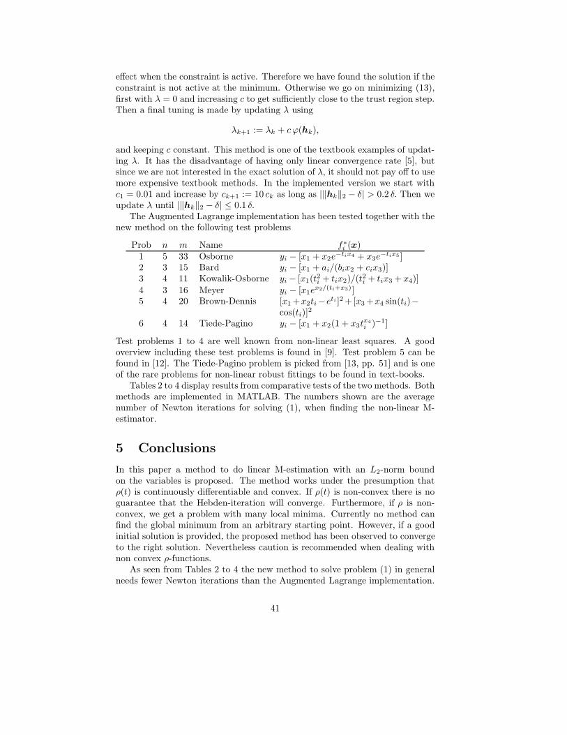
The Augmented Lagrange implementation has been tested together with thenew method on the following test problems

Prob n m Name f∗i (x)1 5 33 Osborne yi − [x1 + x2e

−tix4 + x3e−tix5 ]

2 3 15 Bard yi − [x1 + ai/(bix2 + cix3)]3 4 11 Kowalik-Osborne yi− [x1(t2i + tix2)/(t2i + tix3 + x4)]4 3 16 Meyer yi − [x1e

x2/(ti+x3)]5 4 20 Brown-Dennis [x1 +x2ti−eti ]2 +[x3 +x4 sin(ti)−

cos(ti)]2

6 4 14 Tiede-Pagino yi − [x1 + x2(1 + x3tx4i )−1]

Test problems 1 to 4 are well known from non-linear least squares. A goodoverview including these test problems is found in [9]. Test problem 5 can befound in [12]. The Tiede-Pagino problem is picked from [13, pp. 51] and is oneof the rare problems for non-linear robust fittings to be found in text-books.

Tables 2 to 4 display results from comparative tests of the two methods. Bothmethods are implemented in MATLAB. The numbers shown are the averagenumber of Newton iterations for solving (1), when finding the non-linear M-estimator.

5 Conclusions

In this paper a method to do linear M-estimation with an L2-norm boundon the variables is proposed. The method works under the presumption thatρ(t) is continuously differentiable and convex. If ρ(t) is non-convex there is noguarantee that the Hebden-iteration will converge. Furthermore, if ρ is non-convex, we get a problem with many local minima. Currently no method canfind the global minimum from an arbitrary starting point. However, if a goodinitial solution is provided, the proposed method has been observed to convergeto the right solution. Nevertheless caution is recommended when dealing withnon convex ρ-functions.

As seen from Tables 2 to 4 the new method to solve problem (1) in generalneeds fewer Newton iterations than the Augmented Lagrange implementation.

41

Table 2: Average number of Newton iterations for solving the linearized model in

non-linear Lp-estimation.

Problem 1 2 3 4 5 6

p = 2 New method 1.7 1.3 1.2 1.5 1.9 1.3Aug. Lag. 6.6 4.8 1.5 3.7 29.4a 1.7

p = 1.75 New method 5.4 6.3 2.6 4.4 2.6 2.8Aug. Lag. 5.5 9.5 2.4 7.5 27.5a 2.2

p = 1.5 New method 6.6 6.6 3.7 6.6 4.9 4.1Aug. Lag. 6.4 8.6 3.2 7.3 27.7a 2.3

p = 1.25 New method 11.5 11.0 4.5 8.0 4.4 11.6Aug. Lag. 23.8 14.9 3.7 10.0 36.1 5.8

a – Maximum number of iterations (non-linear problem)

Table 3: Average number of Newton iterations for solving the linearized model in

non-linear Huber-estimation.Problem 1 2 3 4 5 6

k = 2 New method 2.3 3.0 1.2 2.8 3.0 2.2Aug. Lag. 4.5 5.2 2.1 35.1 27.7 6.8

k = 1.5 New method 2.7 3.8 1.3 2.5 2.9a 2.3Aug. Lag. 4.8 5.2 2.6 23.5 27.7a 4.2

k = 1 New method 2.5 2.5 1.4 1.9 2.2a 1.1Aug. Lag. 13.9 5.0 3.4 – 22.8a 3.9

k = 0.5 New method 4.1 3.0 1.7 2.7 1.9a 1.1Aug. Lag. 15.6 5.3 3.3 5.4 38.9 1.0

a – Maximum number of iterations (non-linear problem)‘–’ – Completely wrong or no result (non-linear problem)

Table 4: Average number of Newton iterations for solving the linearized model in

non-linear Fair-estimation.Problem 1 2 3 4 5 6

k = 3 New method 4.5 5.8 1.9 5.3 2.4a 3.9Aug. Lag. 15.6 8.3 2.4 6.4 28.0 6.4

k = 2 New method 4.7 6.5 2.0 5.6 3.0 4.1Aug. Lag. 15.6 8.0 2.6 6.3 25.0a 4.9

k = 1 New method 4.9 5.7 2.1 6.2 2.7a 4.5Aug. Lag. 17.0 6.9 3.7 6.9 24.5a 5.2

a – Maximum number of iterations (non-linear problem)

42

Since also the computation of the Hessian is simpler, it seems obvious that thenew method is to be preferred.

Acknowledgments

The author wishes to thank Hakan Ekblom and Kaj Madsen for stimulatingdiscussions and valuable comments on this work. He is also grateful to theanonymous referees, whose constructive criticism improved the quality of thepaper.

Appendix

A On Minimizing the Lagrangian Function

A.1 Dealing with a Singular System

When the Newton step is calculated with λ = 0, the system of equations maybe singular. This will be detected during the Cholesky-factorization of thesystem matrix. Since we still need to be able to solve this system, we apply aregularization by adding ε1I to the matrix. Thus we obtain(

1σ2JTD(h)J + ε1I

)∆h = − 1

σJTv(h).

In practice it has been observed that ε1 = 1σ2 5εmach‖JTD(h)J‖ works well.

There are other ways of dealing with this too. If the the system is consistent,we can compute the minimum norm solution, and if the system is inconsistentwe can make an orthogonal projection of the negative gradient onto the null-space of the system matrix. Regretfully, these both alternatives involve morecomputations. An interesting observation though is that this is the situation wereach if we let ε1 → 0 in the above system.

A.2 Convergence Criteria

What follows is a description of the implemented convergence criteria for theminimum of (6). We have the algorithm

while∥∥ ∂∂hgλ(h)

∥∥∞ > ε2

solve ( 1σ2J

TD(h)J + 2λI)∆h = − 1σJ

Tv(h)− 2λhperform a line search to obtain αh := h+ α∆h

endwhilehk := h.

43

The stop criterion is based on comparing the length of the gradient with theorder of magnitude of the rounding error in calculating ∂

∂hgλ(h). From [6] weget that the rounding error is approximately bounded by∥∥fl( ∂

∂hgλ(h))− ∂∂hgλ(h)

∥∥∞

<∼εmach(m‖J‖1‖v(h)‖∞/σ + n2λ‖h‖∞) +O(ε2mach).

We use this bound, but with a user supplemented ε3 instead of εmach , to makeit possible to solve with lower accuracy if that is called for. This gives that

ε2 = ε3(m‖J‖1‖v‖∞/σ + n2λ‖h‖∞).

A.3 The Line Search Procedure

To ensure convergence, a line search procedure is needed. The term “line search”corresponds to searching in the direction of ∆h to find an α > 0, such thath+ := h + α∆h results in a gλ(h+) that is considerably smaller than gλ(h).Because of the arbitrary ρ-function, we do not have any special structure in theproblem to take advantage from. Therefore the general line search procedurefrom [4, pp. 33–36] is used. The method will be described in a slightly differentway, but the algorithm is actually the same. It consists of two parts. In the firstpart, a bracket containing the minimum is found. In the second part, the bracketis made smaller until the convergence criterion is met. We use the Wolf-Powellconditions, but with the modification of Fletcher [4] to indicate convergence.Following Fletcher we write g(α) for gλ(h + α∆h), so e.g. g(0) corresponds togλ(h). The modified Wolf-Powell conditions to be fulfilled are

g(α) ≤ g(0) + α%g′(0) (14)

and

|g′(α)| ≤ −ςg′(0). (15)

The constants % ∈ (0, 1/2) and ς ∈ (%, 1) can be chosen arbitrarily within theintervals. Typically we will let % = 0.01. The choice ς = 0.1 is considered as afairly accurate line search and ς = 0.9 is considered as a weak line search. Tocalculate g(α) and g′(α) we define

k1 = λ(hTh− δ2),k2 = 2λhT∆h,k3 = λ∆hT∆h,

r(0) = l(h)/σ and∆r = J∆h/σ.

We will calculate

r(α) = r(0) + α∆r

g(α) =m∑i=1

ρ(ri(α)) + k1 + α(k2 + αk3)

44

and

w(α) = [ρ′(ri(α))]mi=1

g′(α) = ∆rTw(α) + k2 + 2αk3.

When we expand the bracket [αleft , αright ], we increase the “right” end of itwith at most τ1 > 1 and at least with 1 times the bracket size. We keep doingthis until g′(αright ) > 0 or g(αright ) ≥ g(αleft) or (15) is fulfilled or (14) is notfulfilled for αright . For every new αright , αleft is set to the old αright .

(* EXPANDING THE BRACKET *)αleft := 0αright := 1αmax := −(λδ2 + g(0))/(%g′(0)) (* g(α) ≥ −λδ2 & (14) ⇒ α ≤ αmax *)calculate g(0), g′(0), g(αright ) and g′(αright )while g(αright) ≤ g(0) + αright%g

′(0) and g(αleft ) > g(αright )and g′(αright ) < ςg′(0) do

if 2αright − αleft ≥ αmax thenαnew := αmax

elseαnew := min. of cubic poly. through g(αleft ), g′(αleft ),

g(αright ) and g′(αright )limit αnew ∈ [2αright − αleft ,min(αmax , αright + τ1(αright − αleft ))]

endifαleft := αright

αright := αnew

calculate g(αright ) and g′(αright )endwhileif |g′(αright )| ≤ −ςg′(0) and g(αright ) ≤ g(0) + αright%g

′(0) thenreturn αright

endif

In the phase when we shrink the bracket, we use the fact that one of the bordervalues of the bracket always is “better” than the other one. We try to keeptrack on this situation by using the border variables αgood and αbad .

if g(αright ) > g(0) + αright%g′(0) or g(αleft) ≤ g(αright ) then

αgood := αleft

αbad := αright

elseαgood := αright

αbad := αleft

endif

The property of being the left or the right border is easily examined by lookingat the values of the border variables. We shrink the bracket by minimizinga polynomial that estimates g(α) through the edges (αgood and αbad) of thebracket. The constants τ2 and τ3 guard against too small steps. The outer

45

loop updates αgood and the inner loop updates αbad until g(αnew ) is better thang(αgood). αnew is the “latest” calculated new edge.

(* SHRINKING THE BRACKET *)cubic := TRUEwhile |g′(αgood)| > −ςg′(0) do

if cubic thenαnew := min. of cubic poly. through g(αgood), g′(αgood),

g(αbad) and g′(αbad)else

αnew := min. of quad. poly. through g(αgood), g′(αgood) and g(αbad)endiflimit αnew ∈ [αgood + τ2(αbad − αgood), αbad − τ3(αbad − αgood)]evaluate g(αnew )while g(αnew ) > g(0) + αnew%g

′(0) or g(αgood) ≤ g(αnew ) docubic := FALSEαbad := αnew

αnew := min. of quad. poly. through g(αgood), g′(αgood) and g(αbad)limit αnew ∈ [αgood + τ2(αbad − αgood), αbad − τ3(αbad − αgood)]evaluate g(αnew )

endwhileevaluate g′(αnew )if (αbad − αgood)g′(αnew ) ≥ 0 then

cubic := TRUEαbad := αgood

endif

We must keep the mini-mum within the bracket

αgood := αnew

endwhilereturn αgood

In the implementation of the shrinking phase, in addition we stop the iterations if(αbad−αgood)g′(αgood) ≤ εmachg(αgood). This condition is proposed by Fletcher[4, pp. 38] to guard against numerical degeneracy.

The parameter values % = 0.01, ς = 0.5, τ1 = 9, τ2 = 0.1 and τ3 = 0.5 areused in the implementation. In [4] there is a global convergence proof for thisline search procedure used with any descent method.

B Some Considerations when Implementing theNon-Linear M-Estimation Algorithm

B.1 Estimating λ when δ is Changed

When δ is changed in the non-linear M-estimation algorithm, the old value ofλ probably gets in error. There are however means to make an estimate of thenew λ. Using a Taylor expansion for the function

ξ(λ) =1

‖h(λ)‖2− 1δ

46

we get

ξ(λ) = ξ(λold) + ξ′(λold)(λ − λold) +O((λ − λold)2).

By skipping the high order term, setting ξ(λ) = 0 and solving for λ, we getthe Hebden iteration (12). But instead of setting ξ(λ) = 0, we can derive anapproximative relation between ‖h(λ)‖2 and λ. Doing this we get

‖h(λ)‖2 =− ‖h(λold)‖22

ddλ‖h(λold)‖2

− ‖h(λold)‖2ddλ‖h(λold)‖2

− λold + λ.

This is actually the same model as the one traditionally used (by e.g. More [12])to derive (12). Since ‖h(λ)‖2 = δ, we thus can make the estimation

λest =‖h(λold)‖2ddλ‖h(λold)‖2

+ λold −‖h(λold)‖22ddλ‖h(λold)‖2

· 1δ.

B.2 Detecting Numerical Degeneracy in the Trust RegionParameter r

In trust region methods the quantity

r =∆f∆q

,

plays an important role in telling the correctness of the “model” in the currenttrust region. The quantity ∆f is the change in the object function and ∆q is thechange in the “model” of the object function. In the algorithm for non-linearM-estimation, r is

r =∑m

i=1 ρ(f∗i (x)/σ)−∑m

i=1 ρ(f∗i (x+ h)/σ)∑mi=1 ρ(fi/σ)−

∑mi=1 ρ(li(h)/σ)

.

In the following, we will instead write

r =∑mi=1 ai −

∑mi=1 bi∑m

i=1 ai −∑mi=1 ci

,

to make the notation simpler. Note that f = f∗(x)When we are getting close to the solution of the non-linear problem, we

may get catastrophic cancellation in both the numerator and the denominator.What we want to do is to calculate r with as small error as possible and todetect when it possibly is subject to catastrophic cancellation.

The sums in the numerator and the denominator are numerically favorableto calculate like

S =m∑i=1

(ai − bi),

47

if ai and bi are close. Using the technique of Wilkinson [14], we find that therounding errors involved when calculating S are bounded by

|fl(S)− S| ≤ (m+ 1)um∑i=1

|ai − bi|+ uam∑i=1

ai + ubm∑i=1

bi +O(u2),

where u is machine epsilon, and ua and ub are bounds for the relative errors inai and bi respectively. In the denominator of r, bi is switched for ci, with uc asthe relative error in ci.

The error bound for S can be used as a safeguard against the effects ofcatastrophic cancellation when calculating r. If only the denominator ∆q issmaller than the error bound we consider the calculation of r to be of the type1/0. The effect of this then should be that the trust region is increased if∆f > 0, and otherwise decreased.

If both the numerator ∆f and the denominator ∆q are smaller than cor-responding error bounds, the calculation is to be considered as 0/0 i.e. we donot know anything about the result. The only reasonable thing to do in thatsituation is to keep the trust region unchanged. Otherwise many successive 0/0situations could cause the region to grow or shrink out of control.

If only the numerator ∆f is smaller than its error bound, we use r = ∆f/∆q.The reason for this is that if there still is some relevant information in ∆f itwill have some effect on r, otherwise not much harm is done by forming r inthat way.

Still the problem remains that we do not know ua, ub and uc. In the Matlabimplementation they are set to ua = ub = 10u and uc = n10u. Other choicesmay be better.

B.3 A Proposal for Non-Linear Lp-estimation

The method for non-linear M-estimation presented in [3, 2] (and in this paper)is not working very well for non-linear Lp problems when p is close to one. Onepossible, but not yet tested, way to get better results in those cases may be tochange the shape of the trust region. Instead of solving (1), we can solve

minimize ‖f + Jh‖psubject to ‖h‖p ≤ δ.

(16)

If we then form the Lagrangian function and add λδp we get

gλ(h) = ‖f + Jh‖pp + λ‖h‖pp =

=∥∥∥∥[ f + Jh

λ1/ph

]∥∥∥∥pp

=

=∥∥∥∥[ f0

]+[

Jλ1/pI

]h

∥∥∥∥pp

.

This is actually an ordinary linear Lp problem that can be solved with thealgorithm of Li [8]. The Hebden iteration is possible to calculate when p > 1, if

48

the same kind of technique is used as in this paper. It is not possible to knowin advance if this is the best method to find λ in the Lp case. The convergenceproof in [3] that is valid for the Ekblom and Madsen method, is not sensitiveto the choice of the norm used for the trust region. This means that it is validalso for these alternative trust regions.

When we have p = 1 the algorithm described in [8] is identical to the Colemanand Li algorithm [1]. Another possibility in the L1 case is to use the algorithmof Madsen and Nielsen [11]. However, there is a high risk that it is not possibleto find a satisfactory solution to (16), when p = 1. In [3] a method is describedcalled “Algorithm 2”, where δ is not used. Instead, λ is updated directly. Thismay be one way to handle the problem with the elusive λ in the L1 case.

References

[1] T. F. Coleman and Y. Li, A globally and quadratically-convergent affinescaling method for linear l1 problems, Mathematical Programming, 56(1992), pp. 189–222.

[2] O. Edlund, H. Ekblom, and K. Madsen, Algorithms for non-linearM-estimation, Computational Statistics, 12 (1997), pp. 373–383.

[3] H. Ekblom and K. Madsen, Algorithms for non-linear Huber estimation,BIT, 29 (1989), pp. 60–76.

[4] R. Fletcher, Practical Methods of Optimization, John Wiley and Sons,second ed., 1987.

[5] P. E. Gill, W. Murray, and M. H. Wright, Practical Optimization,Academic Press, 1981.

[6] G. H. Golub and C. F. Van Loan, Matrix Computations, The JohnsHopkins University Press, second ed., 1989.

[7] M. D. Hebden, An algorithm for minimization using exact second deriva-tives, Report TP515, Atomic Energy Research Establishment, Harwell,England, 1973.

[8] Y. Li, A globally convergent method for lp problems, SIAM J. Optimization,3 (1993), pp. 609–629.

[9] K. Madsen, A combined Gauss-Newton and Quasi-Newton method fornon-linear least squares, Tech. Report NI-88-10, Institute for NumericalAnalysis, Technical University of Denmark, Lyngby 2800, Denmark, 1988.

[10] K. Madsen and H. B. Nielsen, Finite algorithms for robust linear re-gression, BIT, 30 (1990), pp. 333–356.

[11] , A finite smoothing algorithm for linear `1 estimation, SIAM J. Op-timization, 3 (1993), pp. 223–235.

49

[12] J. J. More, The Levenberg-Marquardt algorithm: Implementation and the-ory, in Numerical Analysis, Proceedings Biennial Conference Dundee 1977,G. A. Watson, ed., Berlin, 1978, Springer-Verlag, pp. 105–116.

[13] G. A. F. Seber and C. J. Wild, Nonlinear Regression, John Wiley andSons, 1989.

[14] J. H. Wilkinson, Rounding Errors in Algebraic Processes, H.M.S.O., Lon-don, 1963.

50

Article III

A Piecewise Quadratic

Approach for Solving Sparse

Linear Programming Problems

51

52

A Piecewise Quadratic Approach for Solving

Sparse Linear Programming Problems

Ove Edlund∗1, Kaj Madsen2 and Hans Bruun Nielsen2

1Department of Mathematics,Lulea University of Technology,Sweden

2Department of MathematicalModelling,Technical University of Denmark,Denmark

1 Introduction

In this article we will consider the well-known linear programming problem. Wewill show how to find a solution using piecewise quadratic approximations ofthe dual problem, and we will account for the special treatment that is requiredfor sparse constraint matrices. An implementation in “C” demonstrates theperformance of the algorithm.

The two major players in the area of linear programming algorithms arethe simplex method and the interior point method. The simplex method findsthe solution by a “combinatorial search” for an optimal base in the columns ofthe constraint matrix. The currently most successful interior point approachesaccount for the inequality constraints through a logarithmic barrier functionand use various techniques to speed up Newton’s method. The concept of the“central path” is important in that respect. The central path represents theexact solution corresponding to different slopes of the barrier function. Theimpressing low number of iterations required by the interior point methodsis acquired in part by not actually reaching the central path until the linearprogramming solution is found.

The algorithm presented in this paper has things in common with boththe simplex method and the barrier interior point method. As in the simplexmethod there is a “base” consisting of columns in the constraint matrix. Buthere the number of columns in the “base” may vary, therefore it is not a proper“base” and is thus named active set instead. The use of the active set makes“warm starts” possible in the calculation of the iteration step, and thus drasti-cally reduces the computational work. Also, just like the simplex method, thepresented algorithm is finite.∗Part of this work was done at the Department of Mathematical Modelling at the Technical

University of Denmark. Ove Edlund’s travels and stay were supported by two grants fromNorFA.

53

As with interior point methods, the object function is modified to account forinequality constraints, but instead of barrier functions, we use quadratic penaltyfunctions on the dual problem. In the event of a variable with both upper andlower bounds, the “kink” in the objective function of the dual problem is handledby replacing it and its neighbourhood with a quadratic function. The concept ofthe central path also has meaning here. It corresponds to solutions with differentslopes of the penalty functions, but unfortunately we are still at a stage wherethe central path has to be reached before changing the slope. This puts a severepenalty on the computational efficiency, so the algorithm is currently not quiteup to par with the interior point algorithms.

The algorithm has emerged from a series of articles. Madsen & Nielsen(1990) presented a finite algorithm for solving linear regression problems usingthe Huber criterion. This was accomplished by finding the minimum of a certainpiecewise quadratic function. As part of the Huber criterion, there is a positiveparameter γ. It has the effect that the least squares solution is found as γ →∞,and the `1 solution is found as γ → 0. There is more to it however: Madsen &Nielsen (1993) showed that the `1 solution is found immediately whenever γ issmaller than a certain threshold γ0 > 0, thus it is not required to let γ go to zero.Therefore, by minimizing a sequence of piecewise quadratic approximations ofthe `1 problem for decreasing γ-values, the `1 solution is found whenever γ ≤ γ0

is fulfilled.The step from linear `1 regression to linear programming is short. A linear

programming problem with lower bounds −1 and upper bounds +1 on all vari-ables, has a dual that is a linear `1 estimation problem with a linear term addedto the objective function. This was used in Madsen, Nielsen & Pınar (1996)to further develop the `1 algorithm for this particular class of LP-problems. Arelated approach is found in Pınar (1997), where the theory developed in Mad-sen & Nielsen (1993) and Madsen et al. (1996) is applied on an LP-problem instandard form, when a quadratic penalty function is applied on the dual slackvariables.

In the present article the approaches in Madsen et al. (1996) and Pınar (1997)are unified by considering general lower and upper bounds on the variables inthe primal problem. By selecting lower bounds l = −1 and upper bounds u = 1,where 1 is a vector of all ones, we get the piecewise quadratic functions used inMadsen et al. (1996), and by choosing l = 0 and u =∞ we get the ones usedin Pınar (1997), apart from a constant factor.

Both Madsen et al. (1996) and Pınar (1997) had efficient implementationsof their LP-algorithms, relying on the linear algebra package AAFAC (Nielsen1990) which handles full matrices. In many applications, however, the con-straint matrix is large and sparse. If a problem has that property the imple-mentation should take advantage of it, therefore an implementation of a sparselinear algebra package, tailored for piecewise quadratic optimization has beenmade (Edlund 1999). The sparse software package uses direct methods, sincethe systems solved are likely to be fairly ill-conditioned. The key features arean implementation of an approximate minimum degree reordering algorithm forreducing the number of non-zeros in the factors (Amestoy, Davis & Duff 1996),

54

LQ factorization using a multifrontal algorithm (Matstoms 1994), and updat-ing/downdating of the LQ-factorization.

In section 2 the piecewise quadratic approximation of the dual problem isdescribed. Some properties of the approximation are presented in section 3.The algorithm consists of an inner iteration to get to the “central path” andan outer iteration where γ is decreased, as described in section 4. In section 5some implementational aspects are presented that relate to the sparse natureof the constraint matrix: subsection 5.1 describes the regularization used in thesparse system of linear equations, and subsection 5.2 accounts for the sparselinear algebra used in the implementation. The implementation is applied tosome test problems in section 6 and finally section 7 delivers some conclusions.There is also an appendix with some additional theoretical treatment.

Throughout the paper we use ‖ · ‖ to denote the Euclidean norm.

2 Approximating Linear Programs with Piece-

wise Quadratic Functions

We consider linear programs with upper and lower bounds on the variables. Toallow for simple bounds and free variables, the bounds will be taken from theextended real line, E, i.e. ±∞ is included. Thus given constant vectors c ∈ Rm,l,u ∈ Em, b ∈ Rn and a constant matrix A ∈ Rn×m that is sparse, we want tofind a vector y ∈ Rm that solves

maximize cTy ,subject to Ay = b ,

l ≤ y ≤ u .

(1)

It is well known that the dual problem of (1) is

minimize bTx−∑

li>−∞lizi +

∑ui<∞

uiwi ,

subject to ATx− z +w = c ,

z,w ≥ 0 ,

zi = 0, if li = −∞ ,

wi = 0, if ui =∞ .

(2)

where the vectors x ∈ Rn and z,w ∈ Rm are unknown. The optimal solutionsof (1) and (2) are connected by the duality slackness:

Theorem 1 (Duality slackness) Let y be feasible for (1) and x, z, w befeasible for (2), then they are optimal solutions if and only if

yi > li =⇒ zi = 0 , yi < ui =⇒ wi = 0 ,yi = li ⇐= zi > 0 , yi = ui ⇐= wi > 0 ,

for all indices i = 1 . . .m.

55

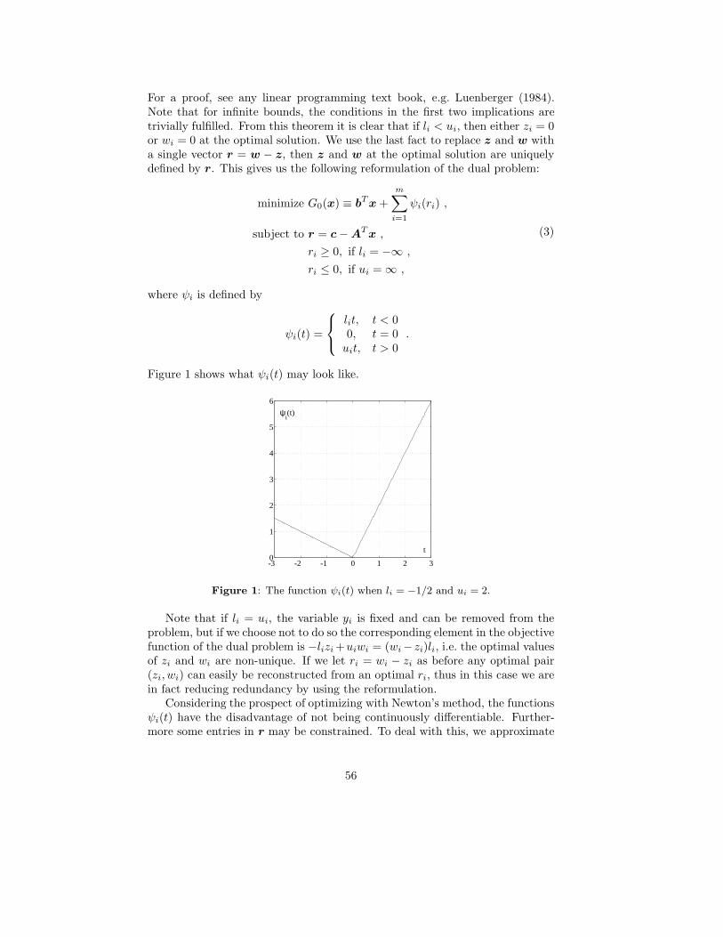
For a proof, see any linear programming text book, e.g. Luenberger (1984).Note that for infinite bounds, the conditions in the first two implications aretrivially fulfilled. From this theorem it is clear that if li < ui, then either zi = 0or wi = 0 at the optimal solution. We use the last fact to replace z and w witha single vector r = w − z, then z and w at the optimal solution are uniquelydefined by r. This gives us the following reformulation of the dual problem:

minimize G0(x) ≡ bTx+m∑i=1

ψi(ri) ,

subject to r = c−ATx ,

ri ≥ 0, if li = −∞ ,

ri ≤ 0, if ui =∞ ,

(3)

where ψi is defined by

ψi(t) =

lit, t < 00, t = 0 .uit, t > 0

Figure 1 shows what ψi(t) may look like.

-3 -2 -1 0 1 2 30

1

2

3

4

5

6

t

ψi(t)

Figure 1: The function ψi(t) when li = −1/2 and ui = 2.

Note that if li = ui, the variable yi is fixed and can be removed from theproblem, but if we choose not to do so the corresponding element in the objectivefunction of the dual problem is −lizi+uiwi = (wi−zi)li, i.e. the optimal valuesof zi and wi are non-unique. If we let ri = wi − zi as before any optimal pair(zi, wi) can easily be reconstructed from an optimal ri, thus in this case we arein fact reducing redundancy by using the reformulation.

Considering the prospect of optimizing with Newton’s method, the functionsψi(t) have the disadvantage of not being continuously differentiable. Further-more some entries in r may be constrained. To deal with this, we approximate

56

-3 -2 -1 0 1 2 30

1

2

3

4

5

6

t

ρi(γ)(t)

γ = 0γ = 0.25γ = 0.75γ = 2

Figure 2: The function ρ(γ)i (t) for li = −1/2 and ui = 2.

ψi(t) with continuously differentiable functions ρ(γ)i (t):

ρ(γ)i (t) =

lit− γ

2 l2i , t < γli

12γ t

2, γli ≤ t ≤ γuiuit− γ

2u2i , t > γui

.

Figure 2 shows how one ψi(t) is approximated by ρ(γ)i (t) for different values of

γ, when ri is unconstrained. If ri is constrained, ρ(γ)i (t) is a penalty function,

that forces the constraint on ri to be fulfilled as γ → 0. This is illustrated inFigure 3.

-3 -2 -1 0 1 2 30

1

2

3

4

5

6

t

ρi(γ)(t)

γ = 0γ = 0.02γ = 0.2γ = 2

Figure 3: The function ρ(γ)i (t) for li = −1/2 and ui =∞. This is a penalty function

that makes ri ≤ 0 as γ → 0.

57

Thus instead of solving (3) we find solutions of

minimize Gγ(x) = bTx+m∑i=1

ρ(γ)i (ri(x)) ,

subject to r(x) = c−ATx

(4)

for decreasing values of γ. Note that since the functions ρ(γ)i (t) are piecewise

quadratic, so will Gγ(x) be.Let

qγ(x) ≡ 1γr(x) =

1γ

(c−ATx

),

and introduce the vector pγ(x) and the diagonal matrixWγ(x) = diag(w(γ)i (x))

defined by

q(γ)i (x) < li : p

(γ)i (x) = li , w

(γ)i (x) = 0

li ≤ q(γ)i (x) ≤ ui : p

(γ)i (x) = 0 , w

(γ)i (x) = 1 .

q(γ)i (x) > ui : p

(γ)i (x) = ui , w

(γ)i (x) = 0

(5)

Then we can reformulate the functions ρ(γ)i (ri) as

ρ(γ)i (ri) = γ

(p

(γ)i (q(γ)

i − 12p

(γ)i ) + 1

2w(γ)i

(q

(γ)i

)2),

giving

Gγ(x) = bTx+ γ(pTγ (qγ − 1

2pγ) + 12qTγWγqγ

). (6)

For the sake of readability we have omitted the argument (x) for pγ , qγ andWγ . To find the minimum of Gγ(x), we search for zero gradients. The gradientof Gγ(x) is

G ′γ(x) = b−A(pγ +Wγqγ

)and the Hessian is

G′′γ(x) =1γAWγA

T .

The Hessian is defined only for x /∈ Bγ ,

Bγ ={x ∈ Rn | ∃i : q(γ)

i (x) ∈ {li, ui}}.

58

3 Properties of Gγ

Fortunately the bulk of the theory developed in Madsen et al. (1996) carries overto the new formulation. This requires, however, that we define the γ-feasiblesign vector sγ(x) with entries

sγi (x) =

−1, q

(γ)i (x) ≤ li,

0, li < q(γ)i (x) < ui,

1, q(γ)i (x) ≥ ui.

This vector has the important property that it gives each quadratic functionregion a unique mark, furthermore it is constant in the solution set of (4). It isonly Theorem 3 in Madsen et al. (1996) that no longer holds, but that is sincethe domain of G0(x) now is a subset of Rn. Fortunately that theorem is notcrucial. The proof of Corollary 3 in Madsen et al. (1996) is not valid eithersince it requires all bounds in the primal problem to be finite. However, it isnot difficult to find an alternative proof, as shown in appendix B.

The theory presented here is to be seen as a complement, and does notaccount for a full theoretical treatment in itself. The presentation below willmake use of the fact that the “smooth” problem (4) is the dual of the followingdamped version of (1),

maximize Hγ(y) ≡ cTy − 12γy

Ty

subject to Ay = b ,

l ≤ y ≤ u .

(7)

In appendix A it is shown that the duality holds. An important consequence ofLemmas 1 and 2 in that appendix, is that (4) has finite solution for every γ > 0if there exists a feasible point for (1).

Theorem 2 Let xγ and yγ solve (4) and (7), respectively. Then, for γ > 0 :

1◦ Hγ(yγ) = Gγ(xγ) ,

2◦ yγ = pγ(xγ) +Wγ(xγ)qγ(xγ) ,

3◦ Hγ(yγ) is a decreasing function of γ ,

4◦ H0(yγ) ≡ cTyγ is a decreasing function of γ ,

5◦ yγ is the unique solution to problem (1) augmented with the constraint‖y‖ ≤ ‖yγ‖ ,

6◦ ‖yγ‖ is a decreasing function of γ ,

7◦ If xγ is feasible for (3) then G0(xγ) ≥ Gγ(xγ) .

Proof The first two points are proved, as part of Theorem 6, in appendix A.3◦ If 0 < γ1 < γ2 then

Hγ1(yγ1) ≥ Hγ1(yγ2

) = cTyγ2− 1

2γ1yTγ2yγ2

≥ cTyγ2− 1

2γ2yTγ2yγ2

= Hγ2(yγ2) .

59

4◦ As the proof of Theorem 2 in Madsen et al. (1996).5◦ Assume that y solves the augmented problem. Then

cT y ≥ cTyγ and ‖y‖ ≤ ‖yγ‖ .

Thus,

Hγ(y) ≥ cTyγ − 12γy

Tγ yγ ,

i.e. y solves (7). Then y = yγ since the strict concavity of Hγ and thelinearity of the constraints imply that the solution is unique.

6◦ Assume 0 < γ1 < γ2 and ‖yγ1‖ < ‖yγ2

‖. Then 4◦ implies cTyγ1≥ cTyγ2

and 5◦ implies cTyγ1≤ cTyγ2

. Hence cTyγ1= cTyγ2

, and thus

Hγ2(yγ2) = cTyγ2

− 12γ2y

Tγ2yγ2

= cTyγ1− 1

2γ2yTγ2yγ2

< cTyγ1− 1

2γ2yTγ1yγ1

= Hγ2(yγ1) ,

which contradicts that yγ2solves (7) for γ = γ2.

7◦ For γ > 0 we have

G0(xγ) ≥ G0(x0) = H0(y0) ≥ H0(yγ) ≥ Hγ(yγ) = Gγ(xγ) .

As a consequence of 2◦ and the strict concavity of Hγ , the sum pγ(x) +Wγ(x)qγ(x) is constant for x in the solution set of (4). In fact, each of thetwo terms in the sum is constant in this set, as a consequence of Lemma 1 inMadsen et al. (1996).

Theorem 3 (From Theorem 4 in Madsen et al. (1996)). If there is a solutionto (4), then there exists γ0 > 0 such that for 0 < γ ≤ γ0 the vectors p = pγ(xγ)and Wq = Wγ(xγ)qγ(xγ) are independent of γ. Thus, if there is a solution to(4), it is characterized by

0 = b−A(p+Wq) ,

where diagi(W ) = 1 =⇒ ri(x0) = 0, and

yγ = p+Wq

is the solution to (1) with minimum Euclidean norm.

Proof If li < qi(xγ) < ui then qi(xγ) is constant because of Corollary 3 inMadsen et al. (1996).

If qi(xγ) ∈ {li, ui} for some i, we can assume that γ0 is so small that

qi(xγ) ∈ {li, ui} =⇒ ri(x0) = 0

Then, the linearity (pγ is constant) implies that qi(xγ) ∈ {li, ui} for all γ in]0, γ0].

Theorem 2 point 5◦ shows that yγ is the solution with minimum norm.

60

In subsection 4.2 it is shown how a solution x0 to (2) is calculated.

4 The Algorithm

The algorithm can be briefly outlined as follows:

Given initial γrepeat

Find xγ = argmin{Gγ(x)} (inner iteration)Reduce γ

until stopping criteria are satisfied

In the discussion we use the so-called active set,

Aγ(x) = {i | w(γ)i (x) = 1} ,

where w(γ)i is defined in (5).

4.1 The Inner Iteration

Since minGγ(x) is an unconstrained convex optimization problem with contin-uous gradient, we find the optimum using Newton’s method with linesearch.The procedure is described in detail in Madsen & Nielsen (1990), but we willreplicate the main ideas.

The Newton-step is found by solving G′′γ(xk)hk = −G′γ(xk), i.e.

AWγAT hk = A

(γpγ +Wγr

)− γb , (8)

where we have omitted the argument xk in Wγ , pγ and r. Since the Newton-step minimizes a quadratic model of the objective function at xk, and ourobjective function is piecewise quadratic, the Newton-step finds the exact min-imum of the quadratic function at xk. If xk ∈ Bγ the step corresponds to theadjacent quadratic function region with most entries in Aγ .

The Newton step is uniquely defined if the matrix Bk = AWγAT is non-

singular, but unfortunately it is very common that Bk is singular when `1- andLP-problems are solved. As in Madsen et al. (1996) we distinguish between thecase where (8) is consistent, and we want the minimum norm solution hm, andthe inconsistent case, where we want ho, the orthogonal projection of the righthand side on the nullspace of Bk. In Section 5.1 we discuss how to implementthis.

If xk+hk and xk are in the same quadratic function region and the system isconsistent, then we are finished and the solution is xγ = xk+hk. Otherwise, wedo a line search. Since we have a continuously differentiable piecewise quadraticfunction, the directional derivative in the search direction hk is piecewise linearand continuous, so it is very simple to find αk so that xk+1 = xk+αkhk satisfies

hTk

(A(γpγ(xk+1) +Wγ(xk+1)r(xk+1)

)− γb

)= 0 .

61

The system (8) is solved via a factorization Bk = LkLTk . Typically, there

is only a modest change between the active sets Aγ(xk) and Aγ(xk+1). Thisis exploited in the iteration: Lk+1 is found by updating Lk instead of doing acomplete refactorization. Some details are given in Section 5.

The algorithm for the inner iteration can now be sketched in pseudo-code.L0 denotes the final factor from a previous iteration (with larger γ-value) andx1 is a starting guess on xγ .

Given L0 and x1

k := 1repeatgk := A

(γp(xk) +W (xk)r(xk)

)− γb

find Lk by updating Lk−1

find hk by solving LkLTk hk = gkfind αk by line searchxk+1 := xk + αkhkk := k + 1

until xk and xk−1 are in the same quadratic function regionreturn xk

In the implementation, numerical tolerances are used when checking the stop-ping criterion.

4.2 The Outer Iteration

In the outer iteration, the parameter γ is decreased and we have to find theminimizer ofGγ(x) for this reduced parameter value. The conditionG ′(xγ) = 0leads to

γG ′(xγ) = γb−A(γpγ +Wγ(c−ATxγ)

)= 0 ,

so that xγ satisfies

AWγATxγ = AWγc+ γ(Apγ − b) .

Now, for some positive δ (δ < γ) assume that Wγ−δ(xγ−δ) = Wγ(xγ) = Wand pγ−δ(xγ−δ) = pγ(xγ) = p, then

AWATxγ−δ = AWc+ (γ−δ)(Ap− b) .

Let the vector v be found as the solution to

AWAT v =1γAWr(xγ) . (9)

Then it follows that xγ−δ = xγ + δv. This is valid only as long as the active setdoes not change, since a change in A will lead to a change in W and p. Nowdefine x(γ−δ) = xγ + δv for all δ ∈ ]0, γ[. The corresponding residual is

r(γ−δ) = c−ATx(γ−δ) = rγ − δd ,

62

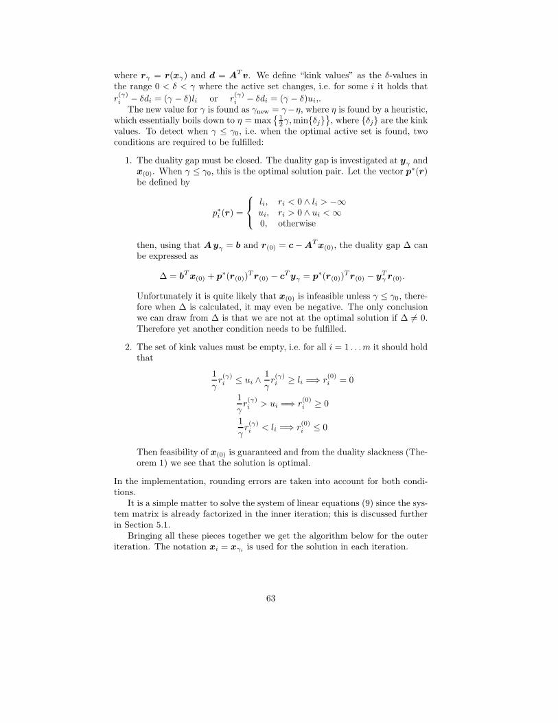
where rγ = r(xγ) and d = ATv. We define “kink values” as the δ-values inthe range 0 < δ < γ where the active set changes, i.e. for some i it holds thatr

(γ)i − δdi = (γ − δ)li or r

(γ)i − δdi = (γ − δ)ui,.

The new value for γ is found as γnew = γ−η, where η is found by a heuristic,which essentially boils down to η = max

{12γ,min{δj}

}, where {δj} are the kink

values. To detect when γ ≤ γ0, i.e. when the optimal active set is found, twoconditions are required to be fulfilled:

1. The duality gap must be closed. The duality gap is investigated at yγ andx(0). When γ ≤ γ0, this is the optimal solution pair. Let the vector p∗(r)be defined by

p∗i (r) =

li, ri < 0 ∧ li > −∞ui, ri > 0 ∧ ui <∞0, otherwise

then, using that Ayγ = b and r(0) = c −ATx(0), the duality gap ∆ canbe expressed as

∆ = bTx(0) + p∗(r(0))Tr(0) − cTyγ = p∗(r(0))Tr(0) − yTγ r(0).

Unfortunately it is quite likely that x(0) is infeasible unless γ ≤ γ0, there-fore when ∆ is calculated, it may even be negative. The only conclusionwe can draw from ∆ is that we are not at the optimal solution if ∆ 6= 0.Therefore yet another condition needs to be fulfilled.

2. The set of kink values must be empty, i.e. for all i = 1 . . .m it should holdthat

1γr

(γ)i ≤ ui ∧

1γr

(γ)i ≥ li =⇒ r

(0)i = 0

1γr

(γ)i > ui =⇒ r

(0)i ≥ 0

1γr

(γ)i < li =⇒ r

(0)i ≤ 0

Then feasibility of x(0) is guaranteed and from the duality slackness (The-orem 1) we see that the solution is optimal.

In the implementation, rounding errors are taken into account for both condi-tions.

It is a simple matter to solve the system of linear equations (9) since the sys-tem matrix is already factorized in the inner iteration; this is discussed furtherin Section 5.1.

Bringing all these pieces together we get the algorithm below for the outeriteration. The notation xi = xγi is used for the solution in each iteration.

63

Get initial γ1 and approximate starting point x∗1i := 1xi = argmin{Gγi(x)} (inner iteration; starting point x∗i )Find vi by (9)while the stopping conditions are not satisfied do

find ηi by heuristicγi+1 := γi − ηix∗i+1 := xi + ηivii := i+ 1,xi = argmin{Gγi(x)} (inner iteration; starting point x∗i )Find vi by (9)

endLet solution x0 := xi + γivi.

In the implementation, the initial solution is found the same way as in Madsenet al. (1996), i.e. by solving

AAT x∗1 = Ac− 12b.

The initial γ1 is found by taking the n:th entry in size of the entries in∣∣r(x∗1)

∣∣.5 Implementation Aspects

The workhorse in the algorithm is the solver for the linear systems (8) and(9). As mentioned, these systems are often rank deficient and in the densematrix case (Madsen et al. 1996) we used the package of Nielsen (1990) toestimate rank and null space basis of the system matrix. This approach is notpractical, however, when the matrix is large and sparse, and we decided touse regularization, see Section 5.1. A detailed description of the sparse matriximplementation is found in Edlund (1999), and in Section 5.2 we give a briefreview of it.

5.1 Regularization

The systems (8) and (9) can be written in the form

Bh = g , (10)

where B = AWγAT is symmetric and positive semidefinite. We replace them

by the regularized systems

(B + µI)hr = g , (11)

where µ is a small positive number, to be discussed later. The matrix B+µI ispositive definite, implying that hr is unique.

64

When (11) is used for finding an approximate Newton step, it is instructiveto note the similarity with Marquardt’s method for nonlinear least squares prob-lems. Let x denote the current iterate and consider the Taylor approximation

Gγ(x+h) ' Gγ(x) +1γψ(h) with ψ(h) = −hT g + 1

2hTBh ,

and g = −γG ′γ(x), B = γG ′′γ (x). The regularized step satisfies

Theorem 4 hr = argmin‖z‖≤‖hr‖{ψ(z)} .

Proof Let φ(z) = ψ(z)+ 12µz

Tz. Then φ′(z) = ψ′(z)+µz = −g+(B+µI)z,which is zero for z = hr. The Hessian matrix φ′′(z) = B+µI is positive definite,so hr is the unique minimizer of φ. Now, let zm = argmin‖z‖≤‖hr‖{ψ(z)}. Thenψ(zm) ≤ ψ(hr), zTmzm ≤ hTr hr, and

φ(zm) = ψ(zm) + 12µz

Tmzm ≤ ψ(hr) + 1

2µhTr hr = φ(hr) .

However, hr is the unique minimizer of φ, so zm = hr.

To analyse the regularization further we introduce the singular value decom-position of the symmetric, positive semidefinite matrix B of rank p,

B = UΣUT , (12)

where the columns {uj} of U ∈Rn×p are orthonormal and Σ = diag(σ1, . . . , σp)with σ1 ≥ · · · ≥ σp > 0. We can write any g ∈Rn as

g = Uα+ gn with α = UTg and UT gn = 0 . (13)

The systemBh = g is consistent if the null space component gn = 0. Especially,this is the case if B has full rank, i.e. when p=n.

Theorem 5 Assume that the system (10) is consistent and let hm denote itsminimum norm solution. Then the regularized solution hr satisfies

‖hr − hm‖ ≤ µ‖B+‖ ‖hr‖ ≤ µ‖B+‖ ‖hm‖ , (14)

where B+ is the pseudo-inverse of B.

Proof Introducing the singular value decomposition (12) we find hm = UΣ−1α,hr = U(Σ+µI)−1α, and

hr − hm =p∑j=1

(1

σj + µ− 1σj

)αjuj =

p∑j=1

−µσj(σj + µ)

αjuj = −µUΣ−1UThr ,

and the first inequality in (14) follows immediately, since ‖B+‖ = ‖Σ−1‖(= σ−1

p

).

The second inequality then follows from Theorem 4.

65

Assume that µ = ε‖B‖ = εσ1. Then the theorem shows that the relativeerror in the step satisfies

‖hr − hm‖‖hm‖

≤ εσ1‖B+‖ = εσ1

σp= εκ2(B) ,

where κ2(B) is the (effective) condition number of B. If ε is a small multipleof the unit round-off, εM, then this error is of the same order of magnitude asthe accumulated effect of rounding errors during the solution of the system. Inthe implementation we use

µ = 500εM‖AW γ‖1‖AW γ‖∞ .

This is simple to compute, and it is easily verified that σ1 ≤ ‖AW γ‖1‖AW γ‖∞.This value should ensure that B+µI is significantly positive definite (also inthe presence of rounding errors), and we shall assume that the problem is sowell-conditioned that the corresponding εκ2(B) < 1. When updating L, wecannot change µ even though W changes. Therefore the desired value of µ ismonitored, and if the difference between the actual and desired value of µ is toobig, a refactorization is done.

In the non-consistent case we want h = ho, the projection of g onto thenull space of B. From (11) and (13) we see that ho = gn and the regularizedsolution is

hr =p∑j=1

αjσj + µ

uj +1µgn .

Thus, if µ � σp and ‖α‖ and ‖gn‖ are of the same order of magnitude, thenhr ' 1

µho, a vector in the right direction. Its actual length is of no importancesince we do a line search.

Once xk is inside the quadratic function region where the solution is, thesolution is approximated by taking two regularized Newton-steps with no line-search. Theorem 5 shows that already after the first step, the error vectorhr − hm is small. Taking yet another full step very likely brings us as close tothe true solution as the conditioning of the problem permits. The extra step inthe quadratic function containing the solution, is equivalent to doing iterativerefinement of the corresponding system of linear equations.

In the implementation, it is assumed that xk is in the solution region ifxk+hk is in the same region as xk. It is required though that the final candidatexk+1 + hk+1 also is in the same region. Numerical tolerances are used whenchecking if two vectors are in the same region.

The regularized matrix in (11) is also used when solving (9) for v. SinceW is idempotent (W = W 2), equation (9) is the normal equation for theoverdetermined problem (WγA

T )v ' 1γr. The system is guaranteed to be

consistent, and by taking a few steps of iterative refinement we can reduce theerror to O

(εMκ2(WγA

T ))

= O(εM

√κ2(B)

), (Bjorck 1987). The iterative

refinement also rectifies the step with regard to the regularization.

66

Finally, the solution of the system (11) is found via a factorization of thematrix, LLT = B + µI, where L is a lower triangular matrix. The straight-forward thing to do here would be to use a Cholesky factorization, but since Lis going to be up- and downdated, and downdating can be ill-conditioned withrespect to the accuracy of the entries in L, another method is used that givesmore accurate entries: LQ-factorization of [AW

õ I], where the orthogonal

matrix Q is discarded. This is feasible since W is idempotent, thus

B + µI = [AW√µ I][AW

õ I]T = LQQTLT = LLT .

Since the LQ-factorization is just the transpose of the QR-factorization, this isa well-known procedure, also in the sparse case.

5.2 Sparse Matrix Considerations

One of the new features in this article, compared to Madsen et al. (1996) andPınar (1997), is the ability to effectively handle sparse linear programming prob-lems. This is done with a sparse linear algebra package, written in C, tailoredfor the algorithm presented above. A detailed description is found in Edlund(1999), and we only give a brief review of the main parts of the package. Fromabove we see that the following features are needed:

• An LQ-factorization of AW , where only L is computed.

• The ability to up- and downdate L as entries in W change.

• Some simple routines for matrix-vector multiplication, forward and back-ward substitution.

The LQ-factorization is just the transpose of the QR-factorization, so thewell-known methods for sparse QR-factorization is directly applicable to ourproblem. The factorization is divided into the following phases:

1. The number of non-zeros in L will depend on the order of the rows ofAW . Therefore, the rows of AW are reordered using the approximateminimum degree reordering algorithm presented by Amestoy et al. (1996).Their algorithm should in fact be applied on AWAT , but as pointed outin George & Liu (1989), it is possible to apply slightly modified minimumdegree algorithms directly on AW . This is done in our implementation.Recently, another implementation also applies the approximate minimumdegree algorithm in the same way as we do (Larimore 1998).

2. Next, the elimination tree is found and the rows of AW are postordered.Modifying a reordering in this way is allowed since the number of non-zeros in L stays intact. The purpose is to prepare for the multifrontalLQ-factorization. This makes it possible to use a stack as intermediatestorage for the dense frontal matrices.

67

3. Once the reordering of the rows ofAW is fixed, the non-zero structure ofLis found. The algorithm for doing this is almost identical to the eliminationtree algorithm, and both are faster than the approximate minimum degreealgorithm.

4. The numerical calculation of the entries in L is then performed with themultifrontal algorithm given in Matstoms (1994). In short, the algorithmidentifies dense sub-problems that are triangularized using Householderreflections. Part of the results from each sub-problem is copied into thestructure of L and the remaining part is then passed to the parent inthe elimination tree. When the whole tree has been traversed the factor-ization is finished. Some techniques are used to speed things up, but tolearn more about “fundamental supernodes”, “node amalgamation” and“block triangular form”, please refer to Matstoms (1994). Despite thesetechniques, the numerical calculation is the most time-consuming phase,just as it ought to be.

As mentioned above the multifrontal algorithm has the nice property that thenumerical calculations are done in dense subproblems. This allows the use ofdense BLAS routines.

Now let us consider sparse updating and downdating. Algorithms for up-dating and downdating are described in e.g. Golub & Van Loan (1989). Therow reordering of AW is found with respect to the current W , and when thischanges one would expect the desired row reordering also to change. However,it is very difficult, maybe even impossible to change the row ordering of L arbi-trarily, without excessive numerical calculations. The strategy that was chosenwas to keep the row reordering fixed in the up- and downdating operations, andthus accepting extra non-zeros in L.

Since the non-zero structure of L may change in each up- and downdateoperation, it is important that the representation of L is dynamic, such thatadding a new non-zero entry can be done with a small amount of work. Still therepresentation should not degrade the performance of the LQ-factorization. Tosatisfy these needs, the columns of L are represented as packed vectors (Duff,Erisman & Reid 1986), with the entries sorted with respect to the row-numbers.The position in memory for any column is not fixed though, so if a column grows,it can easily be copied into a place in memory where it will fit. The “memory”in the implementation is an array whose size is proportional to the number ofnon-zeros in the LQ-factorization.

If memory is filled up with columns, or a downdating is ill-conditioned, thisis signalled back to the calling routine so it can find L by doing a completeLQ-factorization instead. The numerical tolerances used for detecting an ill-conditioned downdate operation are taken from Nielsen (1990).

Performance issues concerning the sparse linear algebra package are dis-cussed in Edlund (1999). The most important shortcoming of the package isthe inability to handle dense columns ofAW γ efficiently. This may be addressedlater.

68

6 Test Results

The tests were run on a Digital Personal Workstation with clock frequency 433Mhz. This means that the peak performance for floating point operations is866 Megaflops. The test problems were preprocessed by rescaling the constraintmatrix A with the algorithm of Curtis & Reid (1972), followed by a rescalingof the columns such that they all had unit length in Euclidean norm. Thealgorithm of Curtis & Reid is applied since many of the testproblems are badlyscaled. The subsequent rescaling of the columns is a heuristic that has provensuccessful in testings. The idea is to make the curvatures of the quadraticfunctions, associated with each column of A, equal.

Running the code on the netlib set of test problems1 generated the resultsin Table 1. The problems “dfl001” and “fit2p” are excluded since they faileddue to shortage of computer memory. With a proper handling of dense columnsin A this would not have happened.

The column “problem” gives the problem names, “time” shows the totalexecution times in seconds, “Mflops” reveals the Megaflops rates. The col-umn “iter” gives the number of iterations defined as the number of changes ofL, either by updating or refactorization, “ref” shows the number of completerefactorizations of L and “red” is the number of reductions of γ. The column γshows the final values of γ and “objval” displays the values of the object functionat the calculated solutions. The marks ∗, ∗∗ and ∗∗∗ indicate that the iterationswere stopped since γ was too small, rather than because of an optimal solutionwas found. The grades “slightly wrong result” and “very bad result” were setby manually comparing “objval” with the objective function values presentedat netlib. The choice of grade for each problem was a matter of judgement onbehalf of the authors.

Table 1: Results for the netlib problems.

problem time Mflops iter ref red γ objval25fv47 15.00 72.53 283 114 24 1.35e-08 5.5018458910e+0380bau3b+ 55.79 47.77 1183 207 23 4.59e-08 9.8730559673e+05adlittle 0.04 26.61 55 4 13 5.79e-04 2.2549496316e+05afiro 0.01 13.54 15 5 6 5.86e-05 -4.6475314286e+02agg∗∗∗ 5.16 62.92 338 97 30 4.77e-11 -4.1445712698e+09agg2∗ 10.38 86.15 397 92 30 8.45e-11 -2.0239252092e+07agg3 9.74 89.55 361 89 26 3.72e-08 1.0312115933e+07bandm 2.08 36.42 371 73 17 2.84e-06 -1.5862801845e+02beaconfd 0.46 32.28 63 20 23 1.25e-09 3.3592485804e+04blend 0.13 32.74 89 25 11 6.00e-06 -3.0812149847e+01bnl1 11.23 47.60 730 220 21 8.21e-11 1.9776275287e+03bnl2 124.14 90.60 1171 352 26 5.11e-09 1.8112365423e+03boeing1 4.32 40.16 329 119 23 8.72e-09 -3.3521356766e+02boeing2 1.10 33.31 388 104 29 5.89e-10 -3.1501882554e+02bore3d 0.62 35.62 119 44 13 3.67e-05 1.3730803942e+03brandy 1.67 49.77 333 79 24 6.08e-08 1.5185098965e+03+ slightly wrong result. ∗∗ too small γ, slightly wrong result.∗ too small γ, but result is good. ∗∗∗ too small γ, very bad result.

1The netlib set of test problems and their descriptions can be found on the internet at<http://www.netlib.org/lp/data/>.

69

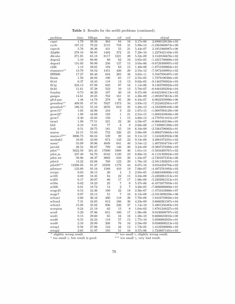
Table 1: Results for the netlib problems (continued).

problem time Mflops iter ref red γ objvalcapri 1.79 39.56 364 84 16 3.17e-06 2.6900129138e+03cycle 187.12 79.22 2115 758 31 5.89e-14 -5.2263868673e+00czprob 5.76 26.36 431 55 21 5.44e-07 2.1851966987e+06d2q06c 278.10 96.95 1482 372 31 7.29e-10 1.2278421103e+05d6cube 271.85 65.18 8117 1221 20 5.52e-09 3.1549166676e+02degen2 5.10 80.86 88 62 10 3.85e-05 -1.4351780000e+03degen3 131.03 99.99 256 127 15 3.05e-06 -9.8729399997e+02e226 1.13 39.65 194 63 15 1.49e-06 -1.8751929062e+01etamacro∗∗ 13.79 58.52 1451 426 29 2.55e-12 -7.5872449991e+02fffff800 17.27 60.48 634 265 38 3.65e-11 5.5567956497e+05finnis 1.50 28.93 190 65 17 2.55e-05 1.7279106560e+05fit1d 0.37 43.43 118 13 13 9.02e-05 -9.1463780924e+03fit1p 223.13 87.98 823 97 16 1.14e-06 9.1463780923e+03fit2d 11.61 37.38 523 10 13 5.78e-07 -6.8464293294e+04forplan 0.73 46.20 187 40 18 9.37e-08 -6.6421884113e+02ganges 14.61 49.25 704 161 31 4.26e-09 -1.0958573613e+05gfrd-pnc 1.48 14.78 278 95 20 8.43e-07 6.9022359996e+06greenbea∗∗ 409.95 47.91 7027 1373 34 3.93e-12 -7.2524822561e+07greenbeb∗∗ 186.54 55.10 2676 653 35 4.28e-12 -4.2335609449e+06grow15∗ 1.05 42.96 216 3 22 1.67e-15 -1.0687094129e+08grow22∗ 1.88 44.88 193 1 21 2.31e-15 -1.6083433648e+08grow7 0.40 45.05 150 1 15 4.60e-12 -4.7787811815e+07israel 1.99 77.51 221 22 20 4.59e-07 -8.9664482186e+05kb2 0.10 9.81 77 8 9 2.60e-06 -1.7499001298e+03lotfi 0.51 29.75 181 55 19 6.10e-09 -2.5264706062e+01maros 24.15 55.83 752 326 23 3.98e-08 -5.8063743663e+04maros-r7∗∗ 3006.73 60.24 539 39 44 9.11e-12 1.5434263924e+06modszk1 10.05 43.89 674 143 22 9.13e-08 3.2061972331e+02nesm∗ 55.09 39.96 4849 641 40 3.54e-12 1.4075934710e+07perold 28.54 86.87 799 146 20 3.24e-09 -9.3807578388e+03pilot∗∗ 5622.59 101.45 17000 1808 40 1.01e-14 -5.5834305767e+02pilot.ja 337.49 94.70 6543 1120 23 8.80e-10 -6.1131393824e+03pilot.we 50.96 48.37 3002 633 20 1.24e-07 -2.7201075354e+06pilot4 13.22 82.08 769 122 29 1.76e-10 -2.5811392637e+03pilot87∗∗ 12398.93 91.27 10339 1179 44 8.07e-16 3.0164494794e+02pilotnov 122.69 95.16 1589 410 19 7.00e-07 -4.4972761892e+03recipe 0.03 38.15 20 4 3 2.05e-05 -2.6661600000e+02sc105 0.09 18.35 84 22 15 3.33e-08 -5.2202061213e+01sc205 0.17 20.97 80 17 17 1.96e-08 -5.2202061212e+01sc50a 0.02 18.23 25 7 9 5.37e-06 -6.4575077059e+01sc50b 0.01 18.72 14 2 7 3.20e-05 -7.0000000000e+01scagr25 0.54 24.36 109 22 18 2.36e-07 -1.4753433060e+07scagr7 0.07 23.14 51 7 16 6.12e-08 -2.3313898238e+06scfxm1 2.60 36.16 460 118 26 7.70e-08 1.8416759028e+04scfxm2 7.31 34.05 612 166 30 4.23e-09 3.6660261567e+04scfxm3 15.08 35.02 896 226 37 1.14e-10 5.4901256483e+04scorpion 0.24 21.19 62 15 8 1.04e-02 1.8781248227e+03scrs8 5.29 37.86 651 180 17 1.96e-06 9.0430098797e+02scsd1 0.15 29.60 65 24 16 1.20e-10 8.6666633016e+00scsd6 0.55 24.24 118 57 15 1.77e-10 5.0500002935e+01scsd8 2.33 29.99 208 76 16 2.58e-09 9.0500000213e+02sctap1 0.56 27.06 124 42 12 1.73e-05 1.4122500000e+03sctap2 2.65 31.97 185 51 16 3.57e-06 1.7248071431e+03+ slightly wrong result. ∗∗ too small γ, slightly wrong result.∗ too small γ, but result is good. ∗∗∗ too small γ, very bad result.

70

Table 1: Results for the netlib problems (continued).

problem time Mflops iter ref red γ objvalsctap3 5.07 33.47 249 76 15 2.45e-06 1.4240000002e+03seba 11.50 102.24 121 21 14 1.18e-05 1.5711600000e+04share1b 0.31 25.56 195 31 21 1.12e-07 -7.6589318579e+04share2b 0.05 31.54 43 4 11 1.05e-05 -4.1573224074e+02shell 2.23 16.43 315 124 21 1.80e-06 1.2088253460e+09ship04l 2.42 18.44 363 152 10 2.85e-03 1.7933245380e+06ship04s 1.70 16.38 294 125 12 2.56e-04 1.7987147004e+06ship08l 4.95 20.32 385 137 10 1.55e-03 1.9090552114e+06ship08s 3.06 18.18 294 121 11 3.14e-04 1.9200982105e+06ship12l 11.17 17.74 684 260 11 3.14e-04 1.4701879193e+06ship12s 3.86 14.77 285 125 11 4.32e-04 1.4892361344e+06sierra∗ 14.49 35.11 564 212 36 1.26e-10 1.5394406931e+07stair 5.53 69.68 361 36 13 2.32e-09 -2.5126695119e+02standata 1.09 25.11 149 51 6 7.35e-03 1.2576995000e+03standmps 1.64 22.66 154 67 8 3.76e-04 1.4060175000e+03stocfor1 0.09 21.30 58 15 12 1.88e-03 -4.1131976219e+04stocfor2 8.99 31.75 283 64 19 8.05e-07 -3.9024408540e+04stocfor3 387.27 26.33 1462 372 26 2.24e-08 -3.9976783846e+04tuff 4.36 51.86 397 171 17 8.97e-12 2.9214776512e-01vtp.base 0.57 25.96 259 71 10 1.64e-04 1.2983146246e+05wood1p 11.46 54.57 523 100 15 4.59e-08 1.4429024320e+00woodw 147.43 57.33 2942 779 9 4.89e-07 1.3044763386e+00+ slightly wrong result. ∗∗ too small γ, slightly wrong result.∗ too small γ, but result is good. ∗∗∗ too small γ, very bad result.

The next set of test problems illustrates the impact the size of the activeset A at the solution, has on the algorithm. The dense constraint matricesare generated by taking as entries uniformly distributed random numbers inthe interval [−1, 1]. We are only investigating the number of iterations. Ifthe computation time was considered, a dense matrix implementation probablywould have been faster. We generate a linear programming problem on standardform,

maximize cTy ,subject to Ay = b ,

y ≥ 0 ,

by first choosing an arbitrary y ≥ 0, with p entries greater than zero. Thenx and r are chosen arbitrarily, but is such a way that the duality slackness(Theorem 1) is fulfilled. If we then use b = Ay and c = ATx+r, the vectors y,x and r are the optimal solutions of the primal and the dual problems. Figure 4shows the number of iterations used for solving such problems, when m = 2nand p is proportional to n.

7 Conclusions and Discussion

The results in Table 1 are both encouraging and discouraging. The good newsis that the code manages to solve many of the netlib problems. The bad newsis that it is not competitive with current interior point codes. Using the public

71

0 100 200 300 400 500 600 700 800 900 10000

50

100

150

200

250

300

m

iter

Figure 4: Number of iterations used by the generated problems.+ : p = 0.8n, ◦ : p = n, × : p = 1.2n

“bpmpd” and “hopdm” codes solves the problems faster and in fewer iterations.The difference is huge for some of the bigger problems, e.g. “stocfor3” is solvedin 18.41 seconds by “bpmpd” using 27 iterations, while the difference is not asbig for the smaller problems, e.g. “scagr25” is solved by “bpmpd” in 0.15 secondsusing 17 iterations. The fact that both “bpmpd” and “hopdm” use presolversto reduce the sizes of the problems also affects the comparison, but only tosome degree. Considering the great amount of research that has gone into theinterior point methods in recent years, the outcome of the comparison shouldcome as no surprise. A strategy for adjusting γ before the “central path” i.e.minxGγ(x) is reached would make for some improvement and would decreasethe gap between the methods. Note that warmstarts appear naturally in thepiecewise quadratic formulation, so the number of iterations need not go downto the level of the interior point methods, for a fast solve. Other things thatmay be possible to improve are the choice of start value for γ, and the initialsolution.

Some of the results in Table 1 suffer from the lack of dense column handling.This is for example true for “seba”. Even though the problem is small andthere is a moderate number of iterations, the solution time still is quite long.This results from the dense columns of A filling up L with non-zeros, causinga tremendous amount of extra work. The multifrontal factorization algorithmdoes its numerical work on dense subproblems, and in this case the whole matrixbecomes one such dense subproblem, giving the high Megaflops rate, but thisdoes not at all compensate for the increased numbers of floating point operationsneeded in the factorization.

Even though the test problems used in Figure 4 are simple to solve comparedto the majority of the netlib problems, it illustrates an important propertyregarding the effectiveness of the algorithm. The algorithm works much betterwith a large active set at the solution than with a small one!

72

When p < n the solution of minxGγ(x) when γ ≤ γ0 is non-unique, and thematrix AW γA

T is singular at the solution. As seen from the figure this is aproblematic case for this algorithm. Unfortunately many of the netlib problemsare of this kind.

The opposite case, when p > n, seems to be very favourable for the algo-rithm. This corresponds to the optimal solution to the primal problem beingnon-unique. The solution yγ , with γ ≤ γ0, then is the minimum norm solution.The success partly is a result from the fact that only one or two reductions ofγ were needed, so the “central path issue” is not a problem here. A successfulγ reduction strategy may show similar performance. Figure 4 suggests thatalready the current algorithm may be a good alternative for solving problemswhere it is known a priori that the primal problem has more than one optimalsolution.

Apart from the things mentioned above, more work is needed to sort outthe issues of the regularization. The current strategy does not deal very wellwith rounding errors at the solution of minxGγ(x) when AW γA

T is singular.It “works” but does not guarantee that the solution is the best possible withrespect to rounding errors.

Another important thing to keep in mind is that the rounding errors in yγare significant if γ is small. This is because it inherits the rounding errors in rscaled with 1/γ. This is not really a problem though, since there are other waysof finding the primal solution if the dual solution is known.

As seen above a lot of work need to be done on this algorithm. Nevertheless,the warm start feature makes it very interesting. The sparse implementation isan important resource for future development. Even the current algorithm maybe competitive for certain classes of problems.

Acknowledgement

The authors would like to thank John Reid for interesting discussions in theareas of sparse linear algebra and rescaling.

Appendix

A Some Remarks on the Duality

In section 3 it was stated that (4) is the dual of (7). Below, this is shown to betrue. In the following, it is assumed that γ > 0.

Lemma 1 (Weak Duality) If y is feasible for (7) and x ∈ Rn, then

Hγ(y) ≤ Gγ(x).

73

Proof Let r = c − ATx, p = pγ(x), W = W γ(x) and A = Aγ(x), thenfrom (6) and (7), and by making use of the fact that cTy = (rT + xTA)y =rTy + xTb we get

Gγ(x)−Hγ(y) = pTr − γ

2pTp+

12γrTWr − rTy +

γ

2yTy

=∑i∈A

( 12γr2i − riyi +

γ

2y2i

)+∑i6∈A

(piri −

γ

2p2i − riyi +

γ

2y2i

).

Investigating each term separately we see that for all i ∈ A,

12γr2i − riyi +

γ

2y2i =

12γ

(ri − γ yi)2 ≥ 0,

and for all i 6∈ A,

piri −γ

2p2i − riyi +

γ

2y2i =

12γ((ri − γ yi)2 − (ri − γ pi)2

)≥ 0.

The last inequality holds since either ri > γui = γpi ≥ γyi, or ri < γli = γpi ≤γyi. Thus Gγ(x)−Hγ(y) ≥ 0 and the lemma follows.

Lemma 2 If Gγ(x) is bounded below, the solution of minGγ(x) is realized ina finite point.

Proof Since Gγ(x) is a continuously differentiable convex piecewise quadraticfunction, consisting of finitely many convex quadratic functions, the minimumobjective function value belongs to some quadratic function. If a convex qua-dratic function is bounded below, it has a minimum that is attained at a finitepoint.

Theorem 6 (Duality) If either (7) or (4) has a finite optimal solution, thenso does the other, and the corresponding values of the objective functions areequal. If xγ and yγ are optimal solutions to (4) and (7) respectively, then

yγ = pγ(xγ) +W γ(xγ)qγ(xγ). (15)

If Gγ(x) is unbounded, then (7) has no feasible point.

Proof The proof of Lemma 1 shows that the duality gap is closed (Gγ(x) =Hγ(y)) if and only if

y = pγ(x) +W γ(x)qγ(x).

Suppose that y fulfils this expression, then from the definitions of pγ(x) andW γ(x), it then is clear that y fulfils the inequality constraints of (7).

Now suppose that (4) has a finite optimal solution. Then it is realized at apoint where G′γ(xγ) = 0, i.e.

b−A(pγ(xγ) +W γ(xγ)qγ(xγ)

)= 0.

74

Let yγ = pγ(xγ) +W γ(xγ)qγ(xγ), then it is clear that yγ is feasible for (7),and finite. Since the duality gap is closed it is also clear that yγ is optimalfor (7).

To prove the converse, suppose instead that y∗γ is an optimal solution of (7)and is finite. Then Lemma 1 implies that Gγ(x) is bounded below, and thusLemma 2 shows that there is a finite optimal solution xγ to (4). Repeatingthe argument above then shows that the objective function values are equalsince Hγ(y∗γ) = Hγ(yγ) = Gγ(xγ) where yγ is defined as above. The proof ofTheorem 2 point 5◦ shows that y∗γ = yγ , thus (15) holds.

To prove the last statement, we note that if Gγ(xγ) is unbounded below,Lemma 1 implies that any finite feasible point in (7) must have an arbitrarilysmall objective function value, which clearly is impossible.

B Additions to the Proof of Corollary 3 in Mad-sen et al. (1996)

Theorem 1 in Madsen et al. (1996) proves that s = sγ(xγ) is constant whenever0 < γ ≤ γ0. The proof of Corollary 3 in Madsen et al. (1996) then relies onthe fact that W sr(xγ)→ 0 as γ → 0, where W s is a diagonal matrix with theentries on the diagonal defined by wii = 1− s2

i , to show that the system

W s

(c−ATz

)= 0

is consistent. The limit has to be re-established though since the entries ofW sr(xγ) no longer are bounded by ±γ. Thus

Lemma 3 If there exists a finite solution to (1), then

limγ→0

W γ(xγ)r(xγ) = 0.

Also, with W s defined as above, it holds that

limγ→0

W sr(xγ) = 0.

Proof Let y∗ be a finite solution of (1). Then from Theorem 2 point 5◦ it isclear that ‖y∗‖ ≥ ‖yγ‖ for all γ > 0. Theorem 6 of appendix A shows thatthere exists xγ such that

yγ = pγ(xγ) +1γW γ(xγ)r(xγ).

Multiplying with W γ(xγ) yields

W γ(xγ)yγ =1γW γ(xγ)r(xγ),

but then

γ‖y∗‖ ≥ γ‖yγ‖ ≥ γ‖W γ(xγ)yγ‖ = ‖W γ(xγ)r(xγ)‖ ≥ 0.

75

Letting γ → 0 in the above expression proves the first limit. Now if 0 < γ ≤ γ0

it holds that

‖W γ(xγ)r(xγ)‖ ≥ ‖W sr(xγ)‖ ≥ 0,

which proves the second limit, as γ → 0.

References

Amestoy, P., Davis, T. A. & Duff, I. S. (1996), ‘An approximate minimum degreeordering algorithm’, SIAM J. Matrix Anal. Appl. 17(4), 886–905.

Bjorck, A. (1987), ‘Stability analysis of the method of semi-normal equationsfor least squares problems’, Linear Algebra Appl. 88/89, 31–48.

Curtis, A. R. & Reid, J. K. (1972), ‘On the automatic scaling of matrices forGaussian elimination’, J. Inst. Math. Appl. 10, 118–124.

Duff, I. S., Erisman, A. M. & Reid, J. K. (1986), Direct Methods for SparseMatrices, Oxford University Press.

Edlund, O. (1999), A software package for sparse orthogonal factorization andupdating. To be submitted.

George, A. & Liu, J. W. H. (1989), ‘The evolution of the minimum degreeordering algorithm’, SIAM Rev. 31(1), 1–19.

Golub, G. H. & Van Loan, C. F. (1989), Matrix Computations, second edn, TheJohns Hopkins University Press.

Larimore, S. I. (1998), An approximate minimum degree column ordering algo-rithm, CISE Tech Report TR-98-016, Dept. of Computer and InformationScience and Engineering, University of Florida, Gainesville, FL. MS Thesis.

Luenberger, D. (1984), Linear and Nonlinear Programming, Addison-Wesley.

Madsen, K. & Nielsen, H. B. (1990), ‘Finite algorithms for robust linear regres-sion’, BIT 30, 333–356.

Madsen, K. & Nielsen, H. B. (1993), ‘A finite smoothing algorithm for linear `1estimation’, SIAM J. Optimization 3(2), 223–235.

Madsen, K., Nielsen, H. B. & Pınar, M. C. (1996), ‘A new finite continuationalgorithm for linear programming’, SIAM J. Optimization 6(3), 600–616.

Matstoms, P. (1994), Sparse QR Factorization with Applications to LinearLeast Squares Problems, Ph.D. dissertation, Department of Mathematics,Linkoping University, S-581 83 Linkoping, Sweden.

76

Nielsen, H. B. (1990), AAFAC, a package of Fortran77 subprograms for solvingATAx = c, Technical Report NI-90-01, Institute for Numerical Analysis,Technical University of Denmark, Lyngby 2800, Denmark.

Pınar, M. C. (1997), ‘Piecewise-linear pathways to the optimal set in linearprogramming’, Journal of Optimization Theory and Applications 93, 619–634.

77

78

Article IV

A Software Package for Sparse

Orthogonal Factorization and Updating

79

80

A Software Package for Sparse Orthogonal

Factorization and Updating

Ove Edlund∗

Department of Mathematics,Lulea University of Technology,

Sweden

1 Introduction

This article will account for an implementation of a software package usingdirect methods for sparse LQ factorization, and updating and downdating ofthe sparse factor L. The factor Q is not considered, since it is of little usein the applications that the software package is aimed for. The name of thesoftware package is spLQ, which is short for “sparse LQ”.

Though it is likely that the software package could be useful in other situa-tions, it has been developed with a certain application in mind. The features in-cluded make up a toolbox for solving piecewise quadratic optimization problems(Madsen & Nielsen 1990, Madsen & Nielsen 1993), and in particular piecewisequadratic approximations of the dual linear programming problem (Madsen,Nielsen & Pınar 1996, Pınar 1997, Edlund, Madsen & Nielsen 1999). The coreof the optimization algorithm is solving systems of the kind

AW kAT hk = gk (1)

where A ∈ Rn×m, W k ∈ Rm×m, hk ∈ Rn, gk ∈ Rn, and m > n. The matrixA is constantly the same, while the other parts of the equation vary from oneiteration to the other. The matrix W k is idempotent and diagonal, with onesand zeros on the diagonal. The indices of the ones correspond to the “activeset” A. One can expect that the active set A changes only marginally betweentwo iterations. Thus the previous factor can be modified with updates anddowndates to reflect the new A. Using this method to find the new factor Lis very cheap, as long as not too much fill-in of L occurs. Another problem isthat the downdating operation may be ill-conditioned, rendering an inaccurateL. Both these potential dangers are handled by occasional refactorizations.∗Part of this work was done at the Department of Mathematical Modelling at the Technical

University of Denmark. Ove Edlund’s travels and stay were supported by two grants fromNorFA.

81

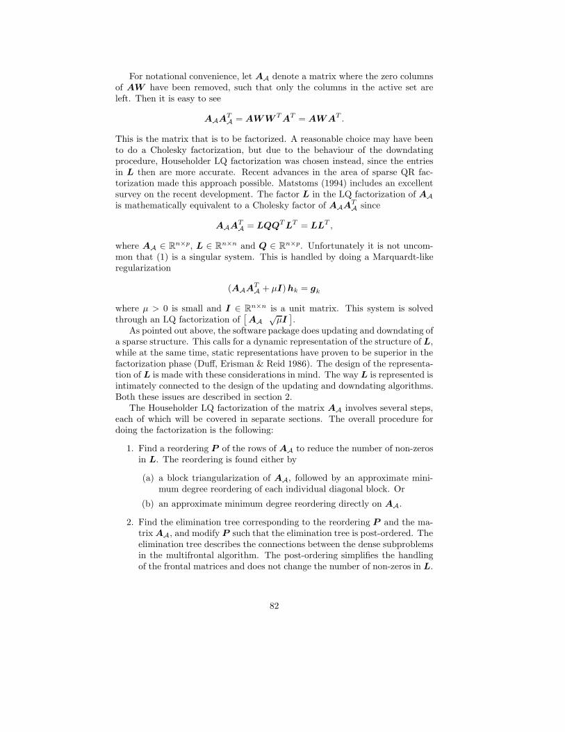
For notational convenience, let AA denote a matrix where the zero columnsof AW have been removed, such that only the columns in the active set areleft. Then it is easy to see

AAATA = AWW TAT = AWAT .

This is the matrix that is to be factorized. A reasonable choice may have beento do a Cholesky factorization, but due to the behaviour of the downdatingprocedure, Householder LQ factorization was chosen instead, since the entriesin L then are more accurate. Recent advances in the area of sparse QR fac-torization made this approach possible. Matstoms (1994) includes an excellentsurvey on the recent development. The factor L in the LQ factorization of AAis mathematically equivalent to a Cholesky factor of AAAT

A since

AAATA = LQQTLT = LLT ,

where AA ∈ Rn×p, L ∈ Rn×n and Q ∈ Rn×p. Unfortunately it is not uncom-mon that (1) is a singular system. This is handled by doing a Marquardt-likeregularization

(AAATA + µI)hk = gk

where µ > 0 is small and I ∈ Rn×n is a unit matrix. This system is solvedthrough an LQ factorization of

[AA

õI].

As pointed out above, the software package does updating and downdating ofa sparse structure. This calls for a dynamic representation of the structure of L,while at the same time, static representations have proven to be superior in thefactorization phase (Duff, Erisman & Reid 1986). The design of the representa-tion of L is made with these considerations in mind. The way L is represented isintimately connected to the design of the updating and downdating algorithms.Both these issues are described in section 2.

The Householder LQ factorization of the matrix AA involves several steps,each of which will be covered in separate sections. The overall procedure fordoing the factorization is the following:

1. Find a reordering P of the rows of AA to reduce the number of non-zerosin L. The reordering is found either by

(a) a block triangularization of AA, followed by an approximate mini-mum degree reordering of each individual diagonal block. Or

(b) an approximate minimum degree reordering directly on AA.

2. Find the elimination tree corresponding to the reordering P and the ma-trixAA, and modify P such that the elimination tree is post-ordered. Theelimination tree describes the connections between the dense subproblemsin the multifrontal algorithm. The post-ordering simplifies the handlingof the frontal matrices and does not change the number of non-zeros in L.

82

3. Do the symbolic factorization, i.e. find the non-zero pattern of the factorL corresponding to AA with row reordering P , without determining thenumerical values.

4. Find the numerical values of the non-zero entries in L by a multifrontalalgorithm. The multifrontal algorithm traverses the elimination tree, anddoes a dense matrix LQ factorization in each node.

The block triangularization makes it possible to do block backward substitu-tion, and thus regarding the square diagonal blocks as dense matrices (Coleman,Edenbrandt & Gilbert 1986, Pothen & Fan 1990). However, this is only feasiblewhen solving linear least squares problems or non-symmetric systems of linearequations. In the context of this article, the “second best” approach is taken.The block triangularization is regarded just as a mean to reduce fill-in in L.This also has the advantage that it is then possible to update and downdate L.The option to skip block triangularization is important when regularization isin use, since the unit matrix in

[AA

õI]

ruins every hope to find a blocktriangularization if AA has rank n. Even if the matrix has lower rank, the unitmatrix still makes the block triangularization useless in practice. Neverthe-less, block triangularization is a fully functional and vital part of the softwarepackage, and is described in section 3.

The minimum degree code is an implementation of the algorithm in Amestoy,Davis & Duff (1996), but instead of applying the algorithm on AAA

TA, the

same kind of reordering is found by only investigating AA, using a techniquedescribed in George & Liu (1989). There is also another recent implementationby T. A. Davis & S. I. Larimore (Larimore 1998), that does essentially thesame as this implementation. In the software package there is also an optionfor the block triangular case, in which the diagonal blocks are considered one ata time, and where the below diagonal non-zeros are taken into account in thedegree calculations. Section 4 describes the implementation of the approximateminimum degree algorithm.

The determination of the elimination tree and the symbolic factorization arecarried out using a technique similar to the one used in the minimum degree al-gorithm. This means that they are applied directly on the sparsity structure ofAA. This is in contrast to Coleman et al. (1986) and Matstoms (1994) where thestructure of AAAT

A is formed before the symbolic factorization. The algorithmsin the software package can be expected to do their work with time complexityO(τL) + O(τAA), where τL and τAA are the number on non-zeros in L andAA respectively, though the theoretical worst case is difficult to determine. Atrivial translation of the minimum degree algorithm gives a symbolic Choleskyfactorization, a procedure that may give non-zero entries in L that should notbe there. By introducing “element counters” the unnecessary non-zeros areremoved from the structure of L. In the case of block triangularization, theelement counters automatically detect block boundaries and thus eliminate theneed for saving information about the diagonal blocks. This also means that itis absolutely essential to enable the use of element counters when block triangu-larization is considered. The use of element counters may cause the elimination

83

tree to split into a forest of elimination trees. The multifrontal factorizationthen automatically traverses each of the trees separately, thus treating each di-agonal block individually. The algorithms for finding the elimination tree anddoing the symbolic factorization are described in section 5.

The implementation of the multifrontal factorization follows Matstoms (1994)closely. For completeness, a short description of the algorithm is found in sec-tion 6, along with some implementational issues.

In section 7 test results are presented, and in section 8 some conclusions canbe found along with some ideas for improvements.

The programming language “C” is used in the implementation. Even though“C” has array indices starting from zero, the notation in this paper is that indicesstart from one, as is the practice in linear algebra for vectors. The translation istrivial. The routines make use of the available data structures in “C”, but onlyto embed the arrays that make up the storage of the sparse matrices. Dynamicmemory allocation is used extensively. This means that the routines only useas much computer memory as is required for their task. Then it is returned tothe operating system for use in other routines. This also means that a potentialuser does not have to guess the amount of memory needed before calling theroutines.

2 Updating and Downdating

When the row reordering of AA is found it is customized for a certain A. AsA changes one would expect the desired row reordering also to change. It ishowever very difficult, and probably impossible, to change the row reordering ofL arbitrarily, without excessive numerical calculations. The strategy that waschosen was instead to keep the row reordering fixed in the update and downdateoperations, and thus accepting extra non-zeros in L.

Since the structure of L may change during every single update and down-date operation, it is very important that the representation of L is dynamic,such that adding a new non-zero entry can be done with a reasonable amountof work. Still the representation should not degrade the performance of theLQ-factorization. What follows is a description of how these goals are fulfilledin the implementation, and a description of the update algorithm.

2.1 Representation of the Lower Triangular L

Experience has shown that the computationally most efficient way of doingsparse factorization is through a symbolic factorization to find the non-zerostructure of the factor, if this is possible, followed by a factorization phase wherethe structure is filled with values (Duff et al. 1986). This makes subsequentupdates and downdates become very difficult, since the non-zero structure willmost likely change when we update or downdate with an arbitrary sparse vector.

To resolve this troublesome situation a dynamic structure is used that ismade up of packed column vectors. Thus the benefit of a static structure is not

84

destroyed and still we have a way of changing the structure, with limited datamovement. The storage for the sparse factor L is designed like this:

• The diagonal is stored in a dense vector, represented by the array d.

• The below diagonal compressed column vectors are stored in the arraysent for the values of the entries, and row for their corresponding rownumbers. These arrays have a length that is equal to the number of non-zeros in L plus, at least initially, some extra space to allow the structureto grow. Looking at element k in the arrays, we have a value ent(k), andthat value resides in row row(k). So we can address rows, but to addresscolumns we need some further information.

• The entries corresponding to a single below diagonal column are storedin consecutive positions in the arrays. The array colp contains the indexwhere each column starts, and endcol points to the first index after thecolumn. So the indices k in ent and row where column cl resides arebounded by colp(cl) ≤ k < endcol(cl). Each column is sorted withincreasing row numbers. An entire column may be moved to anotherposition in ent/row by copying and changing the column position in colpand endcol. Then it is also possible not just to copy, but also to modifythe column as it is moved.

• To be able to move columns around we need to know which positions arefree. This memory management is handled by two arrays freepos andfreesize. The entries in freepos point at the beginning of free blocks inent/row, and freesize contains the number of entries in the same freeblocks. The number of free blocks is stored in the variable freeposlen.There is an upper bound on the number of free blocks stored, in theimplementation it is currently set to 10. Naturally, it is the 10 largestblocks that are stored, and they are sorted in order of increasing blocksize. There is more on the memory management below.

Figure 1 shows an example of this representation. Note that even though thelast column is bound to have only one entry, and that entry is on the diagonal,an empty below diagonal column is included in the structure. This is just toavoid elusive “out of range” errors.

The memory management is handled by a single subroutine, that takes asinput the column number and the new non-zero structure of the column. It isrequired that this non-zero structure is a superset of the old one, i.e. no non-zeros are changed to zeros. The subroutine rearranges the representation of thematrix in such a way that the column gets the new enhanced non-zero structure,but the values do not change. The fresh “non-zero” entries are filled with zeros.So in a mathematical sense the matrix is unchanged, only the storage structureis enhanced. This makes it possible to “rotate” directly into the representationof L instead of into an intermediate storage. The rearranging of memory isperformed using the following principles:

85

L =

26664

1.0 0 0 0 02.0 1.7 0 0 00 −3.0 −2.0 0 00 4.0 0 −4.0 0

5.0 0 0 0.1 6.1

37775

The matrix above can e.g. be represented by

Indices 1 2 3 4 5 6 7 8 9 10d 1.0 1.7 −2.0 −4.0 6.1ent 2.0 5.0 −3.0 4.0 0.1 × × × × ×row 2 5 3 4 5 × × × × ×colp 1 3 5 5 6endcol 3 5 5 6 6freepos 6freesize 5

or by

Indices 1 2 3 4 5 6 7 8 9 10d 1.0 1.7 −2.0 −4.0 6.1ent 0.1 × × × −3.0 4.0 × × 2.0 5.0row 5 × × × 3 4 × × 2 5colp 9 5 1 1 1endcol 11 7 1 2 1freepos 7 2freesize 2 3

Figure 1: A sparse lower triangular matrix and its representation. The symbol ×indicates that the memory space is free.

• If the length of the new column is the same as the old one, they are equaland the matrix is unchanged.

• There may be free storage available right after the current column. If thatfree storage is large enough, the column is extended into it.

• If there is not enough space in the memory management arrays, all columnsare moved to the beginning of row/ent, i.e. a compress is performed. Allthe lost memory that was “leaked” (see below) is recaptured and can beused again. If this does not generate large enough free space, nothingfurther is done and an error is signalled to the calling routine.

• Otherwise, the column has to be copied into a new position. The sortedarray freesize is traversed to find the smallest free space that can hold thecolumn. When the column is moved, new free space is generated wherethe column used to be. If there was an adjacent free space just beforethe new one, the size of that one is increased to incorporate the new freespace. If there was no free space before, one of two things can happen:

– If freeposlen is smaller than its maximum value (in the implementa-tion it is 10), the new free space is added to freepos and freesize.

– If freeposlen is at its maximal value, then the new free space is addedonly if it is larger than the smallest one in freesize. In that case thesmallest space in freesize is dropped from freepos and freesize, i.e.that memory “leaks”. Otherwise the new free memory leaks.

86

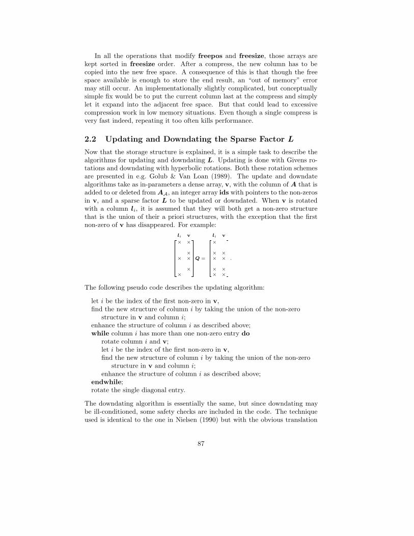
In all the operations that modify freepos and freesize, those arrays arekept sorted in freesize order. After a compress, the new column has to becopied into the new free space. A consequence of this is that though the freespace available is enough to store the end result, an “out of memory” errormay still occur. An implementationally slightly complicated, but conceptuallysimple fix would be to put the current column last at the compress and simplylet it expand into the adjacent free space. But that could lead to excessivecompression work in low memory situations. Even though a single compress isvery fast indeed, repeating it too often kills performance.

2.2 Updating and Downdating the Sparse Factor L

Now that the storage structure is explained, it is a simple task to describe thealgorithms for updating and downdating L. Updating is done with Givens ro-tations and downdating with hyperbolic rotations. Both these rotation schemesare presented in e.g. Golub & Van Loan (1989). The update and downdatealgorithms take as in-parameters a dense array, v, with the column of A that isadded to or deleted fromAA, an integer array ids with pointers to the non-zerosin v, and a sparse factor L to be updated or downdated. When v is rotatedwith a column li, it is assumed that they will both get a non-zero structurethat is the union of their a priori structures, with the exception that the firstnon-zero of v has disappeared. For example:

266666664

li v

× ×

×× ×

××

377777775Q =

266666664

li v

×

× ×× ×

× ×× ×

377777775.

The following pseudo code describes the updating algorithm:

let i be the index of the first non-zero in v,find the new structure of column i by taking the union of the non-zero

structure in v and column i;enhance the structure of column i as described above;while column i has more than one non-zero entry do

rotate column i and v;let i be the index of the first non-zero in v,find the new structure of column i by taking the union of the non-zero

structure in v and column i;enhance the structure of column i as described above;

endwhile;rotate the single diagonal entry.

The downdating algorithm is essentially the same, but since downdating maybe ill-conditioned, some safety checks are included in the code. The techniqueused is identical to the one in Nielsen (1990) but with the obvious translation

87

to hyperbolic rotations. If a hyperbolic rotation turns out to be ill-conditioned,the algorithm stops and an error is signalled to the calling routine, to let it findL by multifrontal LQ-factorization.

In every iteration in the algorithm above, a “symbolic” Givens rotation isdone to find the new structure, i.e. taking the union of the non-zero structurein v and column i. It is then followed by a Givens or hyperbolic rotation to dothe numerical work. This strategy has proven quite successful, but there maybe grounds for criticism. Removing a column from AA should at least let thenumber of non-zeros in L stay the same and possibly decrease. The downdatingalgorithm may however introduce new structural non-zeros inL, and the numberof non-zeros is decreased only if a column is cancelled out by the downdating,which is highly unlikely in practice due to the ill-conditioning of the downdating.It is possible to deal with this by a numerical threshold on the entries in L tofigure out which ones to keep. This constitutes an amount of work proportionalto the number of entries in the new column after a rotation. If only a smallnumber of entries turn zero, this extra work would probably worsen the overallperformance. And after all, ill-conditioning in downdating is so frequent that itis difficult to see the benefits of making things more complicated. In section 7the updating and downdating routines are put to test.

3 Block Triangularization

If the matrix is reducible, it is possible to permute it to a block triangular formwith irreducible square diagonal blocks (Pothen & Fan 1990). This computationis quite inexpensive compared to the other parts of the software package. Theblock triangularization is utilized as a coarse grain factorization that simplifiesthe subsequent factorization work.

The common way of making use of the block triangularization is to solvea system with block backward substitution, see e.g. Coleman et al. (1986) andPothen & Fan (1990). In the spLQ package another approach is taken, which isalso hinted by Coleman et al. Suppose that we have a block triangularization,given by the permutation matrices P 1 and P 2,

P 1AAP 2 =

A11

A21 A22

......

. . .Ar1 Ar2 . . . Arr

,where only Arr has more columns than rows and the other diagonal blocks aresquare. Looking at block column i when i < r, it is obvious that the diagonalblock Aii can be transformed into a lower trapezoidal form with orthogonal

88

transformations by 0Aii

Ai+1,i

...Ari

QTi =

0LiiLi+1,i

...Lri

,

whereQi is an orthogonal matrix of appropriate size and Lii is lower triangular.The complete factorization can then be made by26664

A11

A21 A22

......

. . .

Ar1 Ar2 . . . Arr

37775

26664

QT1

QT2

. . .

QTr

37775 =

26664

L11

L21 L22

......

. . .

Lr1 Lr2 . . .�Lrr 0

�

37775 .

The factorization within one block column is done without using any entriesoutside it. In this respect, the block triangularization is used as a reorderingto reduce the fill-in of L, i.e. reduce the number of additional non-zero entriesproduced by the factorization. A method to reorder for sparsity within a blockcolumn is discussed in section 4.

There are three reasons why this approach is chosen in the software package.

1. It makes it possible to do updates/downdates of the complete matrix L.

2. The package is mainly aimed at solving systems of the kind AAATAh = g.

But block backward substitution is only possible to use on least squaresproblems.

3. The diagonal blocks may be numerically singular. This can be handledthough with the update facility. Thus the importance of being able to doupdates is even more pronounced.

Block triangularization is done in two phases. First a maximum matching isfound, then the block triangular form, or Dulmage-Mendelsohn decomposition,is derived.

Maximum matchings are sometimes referred to as maximum traversals ormaximum assignments (Duff 1981). One way of describing a maximum matchingis that it is a permutation of the rows and columns that gives the longest possiblenon-zero diagonal of a sparse matrix. The number of non-zeros in this diagonalis the structural rank. The true rank of the matrix is always lower than or equalto this structural rank. Figure 3 shows a maximum matching of the sparsitystructure of the matrix in Figure 2. This matrix was generated by randomlypicking a number of columns from the constraint matrix of the netlib linearprogramming problem “25fv47”.

Let τ denote the number of non-zeros in AA, and q be the maximum of thenumber of rows and columns. Then there is an algorithm by Hopcroft & Karp(1973) for finding the maximum matching, that has a worst case complexity of

89

0 100 200 300 400 500 600 700 800 900 1000

0

100

200

300

400

500

600

700

800

nz = 5677

Figure 2: The submatrix of “25fv47” that is used in the examples.

0 100 200 300 400 500 600 700 800 900 1000

0

100

200

300

400

500

600

700

800

nz = 5677

Figure 3: A maximum matching.

90

0 100 200 300 400 500 600 700 800 900 1000

0

100

200

300

400

500

600

700

800

nz = 5677

Figure 4: The block triangularization found by MATLAB.

O(q1/2τ). An efficient implementation of this algorithm is described in Duff &Wiberg (1988). That algorithm is currently the best choice for general sparsematrices. In this software package however, the algorithm of Pothen & Fan(1990) is implemented instead since it is much simpler. Due to Pothen & Fantheir algorithm in general is a little faster than the algorithm of Duff & Wiberg,but sometimes suffers from its worst case complexity of O(qτ).

The second phase, i.e. finding the Dulmage-Mendelsohn decomposition isdone with a modified version of the algorithm in Pothen & Fan (1990). In theiralgorithm, they start off this second phase by doing a coarse decomposition

P ∗1AAP∗2 =

A∗11

A∗21 A∗22

A∗31 A∗32 A∗33

,

where A∗11 (the vertical tail) has more rows than columns, A∗22 is square andA∗33 (the horizontal tail) has more columns than rows. All the structural sin-gularities are gathered in A∗11. The coarse decomposition requires there to be arepresentation of the sparsity structure of AT

A to find A∗11, i.e. O(τ) extra stor-age is needed. After the coarse decomposition, the fine decomposition is doneby applying Tarjan’s algorithm on A∗22, to find smaller diagonal blocks. A gooddescription of Tarjan’s algorithm is found in Duff et al. (1986). The algorithmabove is implemented in the MATLAB kernel as the command dmperm. Figure 4shows the effect of applying dmperm on the matrix in Figure 2. Note that since

91

0 100 200 300 400 500 600 700 800 900 1000

0

100

200

300

400

500

600

700

800

nz = 5677

Figure 5: The block triangularization found by spLQ.

dmperm finds the upper triangular version, the resulting permutations have tobe reversed to get Figure 4. The dotted lines in the figure are the boundaries ofA∗11,A∗22 andA∗33. Notice that most of the diagonal blocks are of size 1×1 in thefigure. This is also the situation in general. Finding the Dulmage-Mendelsohndecomposition has time complexity O(τ), not counting the time needed for themaximum matching.

In the implementation of the Dulmage-Mendelsohn decomposition in spLQ,only the horizontal tail (A∗33) is found during the coarse decomposition. ThenTarjan’s algorithm is applied on the remaining columns. If Tarjan’s algorithmreaches a row without a diagonal entry, or a row that has been marked as be-longing to the vertical tail, then all the entries in the stack of Tarjan’s algorithmare marked as belonging to the vertical tail. In this way it is possible to identifythe vertical tail (A∗11) without forming the structure of AT

A.Furthermore, the implemented algorithm also uses Tarjan’s algorithm to

find diagonal blocks in the vertical tail. This is a great help in the subsequentfactorization. It is important however to point out that those blocks do notshare the same beautiful properties as the ones found in A∗22, since their sizedistribution changes with the initial row and column reordering, thus they arenot optimal.

Figure 5 shows the effect of applying the above algorithm on the matrix ofFigure 2. The important difference to Figure 4 is that the vertical tail (A∗11) ismuch better suited for LQ-factorization. The implementation in spLQ is slightlyslower than the MATLAB implementation. However, the time spent in theseroutines is such a small fraction of the overall factorization time that there wasno reason to optimize them further.

92

4 Approximate Minimum Degree

To limit the number of non-zeros in the sparse factor L, the rows of AA arereordered. This means that PAA = LQ and thus PAAAT

APT = LLT , where

P is a permutation matrix with the reordering. This L is mathematically iden-tical to the Cholesky factor of PAAAT

APT , apart from the sign of some entries.

Therefore, a reordering that is good for Cholesky factorization should also begood for sparse LQ-factorization. The approximate minimum degree orderingalgorithm by Amestoy et al. (1996) is used for finding this row reordering. Theapplication of their algorithm to AAAT

A would require the formation of thenon-zero structure of that matrix. This may be time consuming though, andthe size of AAAT

A is almost at costly to predict. However, it is possible to useminimum degree algorithms by only considering the structure of AA, as pointedout in George & Liu (1989), and that is how it is done in spLQ. Another recentimplementation by T. A. Davis & S. I. Larimore (Larimore 1998) also appliesthe approximate minimum degree algorithm in this way.

George & Liu (1989) and Amestoy et al. (1996) give good presentations of thedetails of the minimum degree algorithm. Only a brief sketch will be presentedhere. The minimum degree algorithm monitors the process of Cholesky factor-ization to determine the permutations. The row in the matrix being factorized,that has the least number of non-zero entries (i.e. the lowest degree), will also beeliminated with the fewest number of floating point operations. Thus this rowis chosen first and the structure is updated according to the corresponding elim-ination. Then we are ready to pick the next row using the same criterion. Thissimple basic algorithm turns out to be quite slow indeed, when implemented.Various strategies to improve performance have been suggested over the years,as summarized in George & Liu (1989). They give an example where thesestrategies give a speed-up by a factor 50. Some of them are described below.

To understand the algorithm, the graph of the matrix is important. Eachnode, or variable, in the graph corresponds to a row in the matrix. The numberof edges connected to a variable is the degree of the variable. When a variableis eliminated, all its connected neighbours will be connected to each other.

One strategy to improve performance is to keep the structure after the re-ordering, and let the removed variable become an “element”, or “eliminatednode”. The recalculations of the degrees become more complicated, but thebookkeeping cost for the structure is much smaller. The net result is a fasteralgorithm. The resulting graph, with variables and elements, is called a quotientgraph. When a new variable is eliminated, it and its connected elements becomea new single element by taking the union of their edges. Thus two elements arenever connected in the graph. In the approximate minimum degree algorithm ofAmestoy et al. (1996) the recalculation of the degrees surrounding an element isvery fast since only approximations, albeit good approximations, of the degreesare calculated.

Now let the rows of our matrixAA be variables and the columns be elements.As seen from Figure 6, the resulting quotient graph is also the bipartite graph ofthe matrix. Now if the elements are removed and replaced by edges, we get the

93

2

4

7

6

5

6

3

3

5

1

2

1

4AA =

× ×

× ××

× × ×× × × ×× × ×

Figure 6: A quotient graph and the corresponding sparsity structure. Variables are

thin lined circles and elements are heavy lined circles. Each entry in AA is an edge

between a variable and an element, i.e. between a row and a column.

4

6

5

3

1

2 AAATA =

× ×× × ×× × ×

× × ×× × × × ×

× × × ×

Figure 7: The graph and structure of AAATA.

structure of AAATA, as demonstrated in Figure 7. So applying the algorithm to

the quotient graph of AA is equivalent to applying it to the graph of AAATA.

The degree approximations are calculated for all variables surrounding an el-ement. To calculate the approximate degrees, we first investigate the number oftimes each element, that is two edges away from the current element, is reached.If we use the quotient graph in Figure 6 as an example, and want to calculate theapproximate degrees of the variables surrounding element 2, we reach element3 once, element 4 twice, element 5 once, element 6 once and element 7 twice.Those numbers are also displayed in Figure 8. Now give the original elementthe number one, then the approximate degrees of the surrounding variablesare found by summing up the number of edges of adjacent elements minus the“numbers” associated with the edges. The example in Figure 8 then gives thatvariable 4 has approximate degree (3− 1) + (2− 2) + (2− 2) = 2, for variable 5it is (3−1)+(2−1)+(3−1)+(2−2) = 5, and for variable 6 the approximationis (3 − 1) + (2 − 1) + (2 − 2) = 3. Comparing these degree approximations toFigure 7, we see that they are the same as the true degrees, except for variable5 whose true degree is 4.

In Amestoy et al. (1996) the initial degrees are immediately found fromthe symmetric matrix, but the quotient graph of the matrix AA does not giveany immediate way to figure out the degrees. One alternative would be tocalculate approximate degrees using some set of elements to include all variables.

94

2

4

7

6

5

6

3

3

5

1

2

1

4

2

2

1

1

1

2

5

3

Figure 8: The number of times the elements are reached in two steps from element

2 and the generated approximate degrees of the variables.

Larimore (1998) instead uses the rather inaccurate but easily calculated degreeapproximations of MATLAB’s “colmmd” (Gilbert, Moler & Schreiber 1992) asstarting guesses of the degrees. The other end of the scale would be to start outwith calculating the true degrees of AAAT

A, by forming its non-zero structure,one column at a time, and take note of the column lengths. This last approachis in fact used in the implementation, since it was not possible to reproduce thegood results of Davis & Larimore with their starting guesses.

The overall principle in the minimum degree algorithm is to find a variablewith minimum degree, eliminate that one, absorb the surrounding elementsinto a single new element that is their union, and recalculate the degrees of thevariables which surround the new element. This is repeated until all variableshave been eliminated. The order in which this has been done make up thereordering of the rows/variables of AA.

In the implementation of this algorithm some techniques are used to makethe elimination process less time-consuming and to improve the quality of thereordering. “Aggressive” element absorption deletes elements whose set of con-nected variables is a subset compared to some other element. This is discoveredwhen the “number” associated with an element is equal to the number of edges.In Figure 8, this is the case for element 4 and 7, thus they can be deleted as theyare subsets of element 2. Variables with equal sets of neighbours are bundledtogether as a supervariable. In the degree calculations, this variable is treatedas if it was single, a technique named “external degree”. If the element absorp-tion results in a variable having only one edge, and that edge goes to the newelement, the variable in question should have been part of the newly eliminatedsupervariable, and can thus be eliminated immediately. This technique is called“mass elimination”. Aggressive element absorption, supervariables and masselimination reduce the size of the problem and make the algorithm progressfaster. The use of external degree improves the quality of the reordering.

Now let us look into some implementational issues. Before starting the actualalgorithm, the structure of AA is copied to a representation that is made upof a set of packed vectors representing the rows of AA, i.e. the adjacency listof the variables, and another set of packed vectors representing the columns ofAA, i.e. the adjacency lists of the elements. No numerical values are storedsince they are not used in the algorithm. This structure makes it easy to find

95

0 100 200 300 400 500 600 700 800

0

100

200

300

400

500

600

700

800

nz = 132495

Figure 9: Sparsity pattern of the factor L without reordering.

the degree approximations described above.When a variable is eliminated from the structure the corresponding row

is traversed, and the patterns of the columns with non-zeros in that row arereplaced by a single column with the union of their patterns. New free spacehas to be found for the adjacency list of the new element, in the representationof the quotient graph. To achieve this a technique similar to the one in Amestoyet al. (1996) is used. Note that the number of non-zeros in the new element issmaller than the sum of non-zeros in the old ones. Thus the total number ofnon-zeros decreases in every elimination.

Also the representation of the variables has to be modified. The implemen-tation does this by traversing the new element to figure out which rows aremodified. Then for each row the old column numbers are replaced by the singlenew one, by shifting the packed vectors. Note that the length of the adjacencylists of the variables will always decrease or stay the same.

To demonstrate the effect of the implemented algorithm we factorize thematrix in Figure 2. The sparsity pattern of the factor L without reordering isshown in Figure 9. With the approximate minimum degree ordering followed bya post-ordering of the elimination tree we get the sparsity pattern of Figure 10.

There is a special approximate minimum degree routine available in spLQ,for the case when block triangularization is used. The routine carries out min-imum degree calculations one block column at a time. Suppose we have the

96

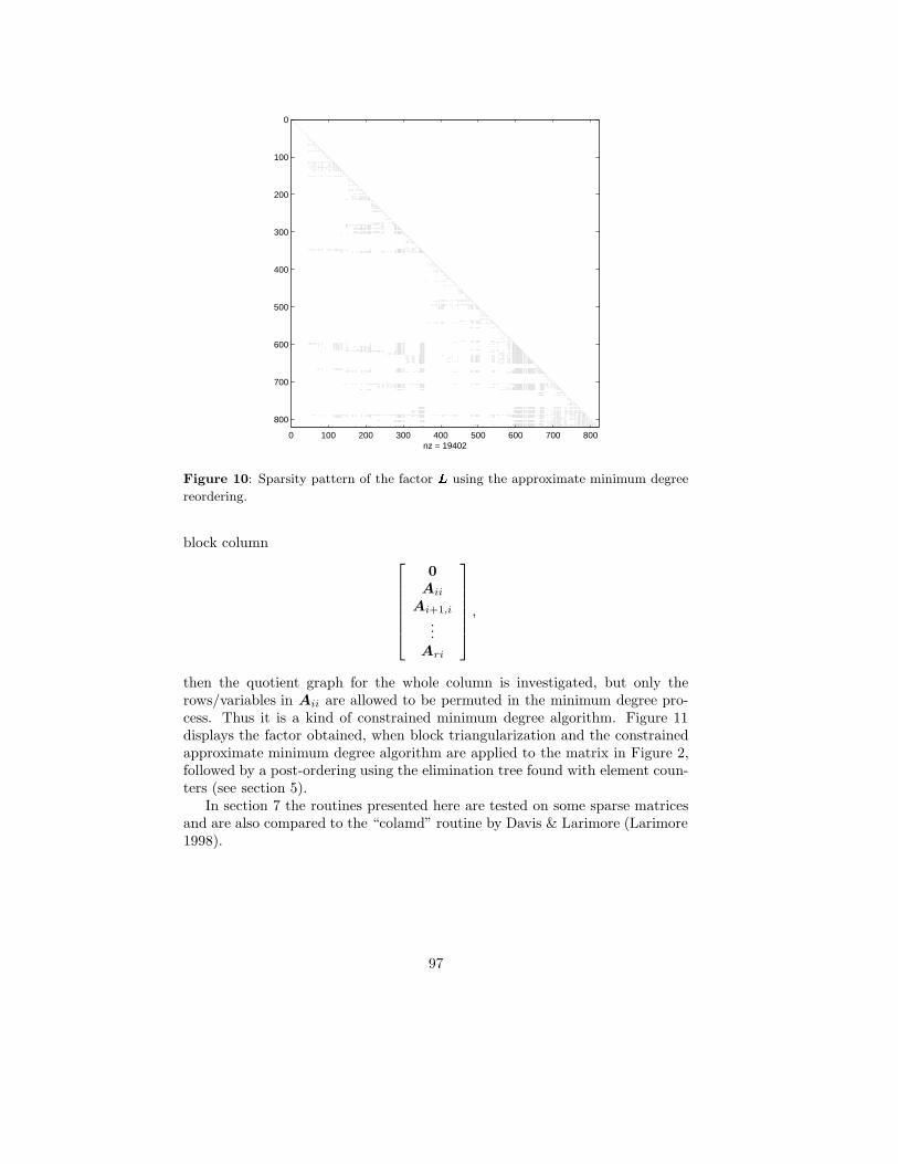
0 100 200 300 400 500 600 700 800

0

100

200

300

400

500

600

700

800

nz = 19402

Figure 10: Sparsity pattern of the factor L using the approximate minimum degree

reordering.

block column 0Aii

Ai+1,i

...Ari

,

then the quotient graph for the whole column is investigated, but only therows/variables in Aii are allowed to be permuted in the minimum degree pro-cess. Thus it is a kind of constrained minimum degree algorithm. Figure 11displays the factor obtained, when block triangularization and the constrainedapproximate minimum degree algorithm are applied to the matrix in Figure 2,followed by a post-ordering using the elimination tree found with element coun-ters (see section 5).

In section 7 the routines presented here are tested on some sparse matricesand are also compared to the “colamd” routine by Davis & Larimore (Larimore1998).

97

0 100 200 300 400 500 600 700 800

0

100

200

300

400

500

600

700

800

nz = 15018

Figure 11: Sparsity pattern of the factor L using block triangularization and con-

strained approximate minimum degree reordering.

5 The Elimination Tree and the Symbolic Fac-torization

The elimination tree gives the dependencies between the dense subproblemswhich are solved in the multifrontal algorithm. The symbolic factorization findsthe sparsity structure of L before the actual factorization. Both of them arefound using essentially the same algorithm.

The common method is to apply the algorithms developed for Choleskyfactorization, and should thus be applied on AAAT

A. But as with the minimumdegree algorithm, it is advantageous if there are algorithms that can be appliedto AA directly. The methods presented here are derived from the approximateminimum degree algorithm of section 4 that operated on AA. Furthermore,with a simple and cheap counting scheme on the elements we will get rid ofthe over-estimation of the sparsity structure that Cholesky related methodsmake. As a consequence, if block triangularization is used in the way proposedin section 3, the column reordering is not needed any longer after finding theminimum degree ordering of the rows, since the other routines will detect blockboundaries automatically.

The fundamental operation is the symbolic Householder reflection which isapplied repeatedly to triangularize AA. First let us reorder the columns of AAto a staircase form, such that columns with entries in the first row are pickedfirst, remaining columns with entries in the second row are picked next, and so

98

on. See Figure 12 for an example. Reordering of the columns of AA has noeffect on L since AAPP TAT

A = AAATA, where P is any permutation matrix.

1

3

2

4 6

5

7

4

5

6

3

2

1

× × ×× ×× × ×

× ×× × ×

× ×

Figure 12: A quotient graph and the corresponding sparsity structure after reordering

the columns to a staircase form.

Applying a Householder reflection on the first row ofAA will make its struc-ture contaminate all other rows that have a non-zero entry in the same columnas some non-zero in the first row. See Figure 13 for an example. The subse-quent reflections will have no further effect on the first column, meaning that thestructure is identical to the first column of L. To find the rest of the columns,the procedure is repeated on the remaining part of the matrix.

2666664

×××× ××××× ×

×××× ×

3777775−

2666664

×××× ××××× ×

×××× ×

3777775

266666664

×××

377777775

�×××

�=

2666664

◦◦ ××◦ ×××◦ ×××

×××◦ ×× ×

3777775

Figure 13: The effect of a symbolic Householder reflection.

Let us look at the representation of this in a quotient graph. Perhaps it wouldbe more appropriate to denote it a bipartite graph, but the notation of section 4will be adopted to avoid confusion. Considering the matrix discussion above,it is obvious that the symbolic Householder reflection to eliminate variable vcorresponds to doing the following in the quotient graph:

1. Form a new element as the union of the elements surrounding variable v.

2. Replace all the elements surrounding v with the new element.

3. Remove variable v and one of the surrounding elements from the graph.

If the variables are eliminated in increasing row number order, the elementsformed in step 1 above will represent the below diagonal structure of the cor-

99

responding column in L. Applying the symbolic Householder reflection on Fig-ure 12, gives the graph in Figure 14.

3

4 6

5

7

4

5

6

3

2

2

◦◦ × ×◦ × × ×◦ × × ×

× × ×◦ × × ×

Figure 14: A quotient graph and the corresponding sparsity structure after the elim-

ination of variable 1. The entries “◦” are not part of the graph. They represent the

sparsity structure of L.

The repetition of identical elements/columns is difficult to handle when im-plemented, since the required size of the structure is not known a priori. It alsogives a degrade in performance. However, the repetition can easily be avoidedby only storing one of the identical elements and introducing an element counteron this single element. Initially all elements will have count 1. When a newelement is formed it will be granted a count, that is the sum of the counts inall the elements surrounding the eliminated variable, minus 1. The minus 1corresponds to the single element going to the structure of L. If it happensthat an element ends up with count zero, that element indeed contributes tothe structure of L, but it will have no further impact on the structure of L andis thus removed from the graph.

32

4

1

61

51

71

4

5

6

3

2

2 1 1 1 1

◦◦ ×◦ × ×◦ × ×

× × ×◦ × ×

Figure 15: A quotient graph and the corresponding sparsity structure after the elim-

ination of variable 1, using element counters to avoid duplication of elements.

Using element counters, the graph in Figure 14 is reduced to Figure 15.When variables 1, 2 and 3 have been eliminated we have Figure 16. When

100

variable 4 is eliminated, the count on element 4 is reduced to zero, and itdisappears as in Figure 17.

4

1

61

51

71

4

5

6

1 1 1 1

◦◦ ◦◦ ◦ ◦◦ ◦ ◦ ×

◦ × × ×◦ ◦ ◦ × ×

Figure 16: A quotient graph and the corresponding sparsity structure after the elim-

ination of variables 1, 2 and 3.

61

51

71

5

6

1 1 1

◦◦ ◦◦ ◦ ◦◦ ◦ ◦ ◦

◦ ◦ × ×◦ ◦ ◦ ◦ ×

Figure 17: A quotient graph and the corresponding sparsity structure after the elim-

ination of variables 1, 2, 3 and 4. Element 4 disappeared since its count turned zero.

Considering that a variable and the surrounding elements are eliminatedand replaced by a new element that is the union of the surrounding elements,we see that this procedure is identical to the elimination in section 4. Thusif the concept of element counters is removed from this scheme, we in factdo a symbolic Cholesky factorization of AAAT

A. The effect of the elementcounters is that elements are removed when they have no further impact onthe Householder reflections. This is useful when the block triangularization ofsection 3 is used, since block boundaries are detected automatically, just givena row reordering of AA. The computational cost for using the element countersis negligible. The overall time complexity for administrating them is O(τAA)where τAA is the number of non-zeros in AA. This is because the adjacencylist for every variable is traversed only once to calculate new element counters,during the whole algorithm. Initially these lists have the total length τAA andtheir individual lengths decrease during the elimination process.

The algorithm for finding the structure of L is implemented in both theroutine for finding the elimination tree and the routine for finding the structureof L. They do however use the information of the sparsity structure in different

101

ways.After eliminating row i, the routine for finding the elimination tree makes the

“parent” of row i equal to the smallest index in the new element. It also sumsthe lengths of all new elements as it goes along, thus determining the numberof non-zeros below the diagonal in L. If element counters are considered and anelement gets count zero the corresponding eliminated row is marked as a rootnode, i.e. it has no parent. In that case we get a forest of elimination trees.

What the routine for finding the structure of L does is obvious. It is howeverimportant to point out that this routine also does a sorting of the row numbersof each column in L.

Both these routines have an option to use or not to use the element counters.As pointed out above, the structure of the Cholesky factor of AAAT

A is found ifthe element counters are not used. It should be possible to incorporate elementcounters also in the minimum degree algorithm. A discussion on this is foundin section 8.

Just as for the minimum degree implementation, packed vectors are usedto represent the adjacency lists of both variables and elements. There is a bigdifference though in how the adjacency lists of the variables are handled. Inthe minimum degree routines the adjacency lists for the rows are being keptcompressed throughout the process. This is a good idea in that case since theyare traversed many times. In the present case however, the adjacency list ofeach variable is traversed exactly once as the variables are eliminated. Therefore,instead of doing a potentially costly shifting of entries in arrays, a boolean arrayis used for marking the elements that have been absorbed. Since the adjacencylists of the variables never grow, traversing these lists takes O(τAA) time.

The element absorption is done by forming the union of the structure ofseveral elements. We have already seen that an element is always either acolumn in AA or a below diagonal column in L. Once an element has beenabsorbed, it “disappears” from the graph. Thus each column in AA is traversedexactly once, and each column of L twice, during the absorptions. I.e. theabsorptions use O(τAA) + O(τL) time, where τL is the number of non-zeros inL. That would also be the time complexity of the algorithm if it was not forone small annoying detail. When a new element gets its index, it is chosen tobe the index of the absorbed element with the highest number of entries, thusthe correct element index is present in a big part of the variable adjacency listscorresponding to the new element, but not all. Those where it is missing haveto be traversed to find an element number that has been absorbed, and thenreplace it with the new index. It is not easy to estimate the amount of workneeded for this, but one can expect it to be modest. So the algorithm shouldbehave as if it had time complexity O(τAA) +O(τL), and in fact it is very fast.

The routine for the post-ordering tries to minimize the size of the stack inthe multifrontal algorithm. It does this by giving each node a weight that isequal to the maximum possible stack size that the node or any of its descendantshave to read into the workspace, and then traverse the children in decreasingweight order when the post-ordering is determined.

102

6 Multifrontal Factorization

Once the row reordering has been settled after block triangularization, approx-imate minimum degree reordering and post-ordering, and the non-zero struc-ture of L has been found, the stage is set for the numerical work. The LQ-factorization in the software package relies on the work of Matstoms (1994), seealso Matstoms (1997). For completeness a rough outline of the algorithm willbe given along with some notes on the implementational strategies.

The numerical values of the entries in L are calculated by traversing theelimination tree and in each node doing a Householder triangularization of thecorresponding submatrix or “frontal” matrix, using dense linear algebra arith-metics. Even though it would be sufficient to eliminate the first row of thefrontal matrix, complete triangularization is favoured since it reduces the sizeof the frontal matrices and thus requires less storage, and reduces the operationcount. At node l, all previously unused columns of AA with entries in row lare collected in a dense frontal matrix. The triangularized frontal matrices ofthe children of node l are also merged into the frontal matrix, such that theindex of the leading nonzero entry of each column increases with the columnnumbers. Matstoms (1994) calls this a BTF (Block Triangular Form), just bearin mind that this is not a block triangularization since the diagonal blocks arenot square. Now using the fact that each Householder vector ends with a lot ofzeros due to the BTF, the operation count for the triangularization of the frontalmatrix can be reduced. After the triangularization, the first column holds thenon-zeros of column l of L. The rest of the dense frontal matrix is sent to theparent in the elimination tree.

The above description induces an order in which the nodes of the eliminationtree have to be traversed; the children have to be traversed before their parents.This happens naturally by traversing the nodes in increasing row number order.To make things even simpler, the depth-first post-ordering makes it possible tostore the submatrices that are sent to the parents, in a stack. The child matricesare read (poped) from the stack, and the submatrix of the dense frontal matrixis pushed to the stack after the triangularization.

If there is a chain with single children in the elimination tree and the struc-ture of the corresponding columns in L match apart from the diagonal elementin each child-parent pair, a fundamental supernode is detected and the chain isreplaced by a single node. This has the practical effect that all the columns corre-sponding to the original nodes may be reported to L after the triangularizationof the frontal matrix. Matstoms (1994) proposes further node amalgamationthat makes the size of the frontal matrices increase. This adds to the operationcount, but improves floating point performance, so that the overall computationtime decreases.

Figure 18 shows the non-zero structure of a matrix and two correspondingelimination trees. In (b), nodes 2, 3 and 5, 6 have amalgamated into two su-pernodes. No further node amalgamation is considered. The progress of themultifrontal algorithm is shown in Figure 19. In Figure 19(a), columns withentries in the first row of AA have formed a dense 3× 2 frontal matrix, corre-

103

4

6

5

31

2

41 2, 3

5, 6

AA =

× ×

× × ×× ×

× × ×× × × × ×× × ×

(a) (b)

Figure 18: (a) The elimination tree of AA. (b) The elimination tree when funda-

mental supernodes are considered.

sponding to node 1 in the elimination tree. Figure 19(b) then shows the frontalmatrix after triangularization. The result in this case is a trapezoidal matrix. InFigure 19(d), two columns of L have been created by the triangularization, cor-responding to the supernode (2, 3) in Figure 18(b). In Figure 19(g), the frontalmatrix corresponding to supernode (5, 6) has assumed its block triangular form(BTF) that makes the triangularization, in this case, a bit cheaper. In generalthe benefits of the BTF are considerable, but this is difficult to achieve in tinyexamples.

All the features described above are part of the implementation. Matstoms(1994) also proposes something called “restricted factorization” to improve float-ing point performance. This feature is not present in the current code, but couldbe a measure to further improve the performance of the multifrontal factoriza-tion.

The implementation makes use of several datatypes. The datatype for the“current” frontal matrix is a dense matrix storage of FORTRAN type, togetherwith a vector containing the row indices of L corresponding to the row indicesin the workspace. Even though the programming language “C” is used in theimplementation, FORTRAN type of dense matrix storage is used here. Thishas a speed advantage since BLAS routines may be used for the Householderreflections.

The entries on the stack are made up of a datatype that essentially is aversion of the workspace, but to save computer memory the triangular or trape-zoidal property of the frontal matrices on the stack is taken into account. Thusthey are stored in a packed format where the diagonal entry and below diag-onal entries of each column are stacked on top of each other in a long array.The stack itself is made up of pointers to such objects. Since dynamic memoryallocation is used, the frontal matrices on the stack have to be allocated beforeentries in the workspace are copied to them, and they have to be deallocatedafter being copied to the workspace.

The BTF of the workspace is built up as columns of AA and the childfrontal matrices are copied into it. Since the elimination tree is represented

104

2666664

2 2

×××× ×

×××2 2 ××××2 2 × ×

3777775

2666664

◦×××× ×

×××◦ 4 ××××◦ 4 × ×

3777775

2666664

◦2 2 2

2 2 2

×××◦ 2 2 2×× 4◦ × ×4

3777775

2666664

◦◦◦ ◦

×××◦ ◦ ◦ 4×× 4◦ × ×4

3777775

(a) (b) (c) (d)

2666664

◦◦◦ ◦

2 2 2

◦ ◦ ◦ 2 2 2 44◦ 2 2 2 4

3777775

2666664

◦◦◦ ◦◦

◦ ◦ ◦ ◦ 4 44◦ ◦ 44 4

3777775

2666664

◦◦◦ ◦◦

◦ ◦ ◦ ◦ 2 2 2

◦ ◦ 2 2 2 2

3777775

2666664

◦◦◦ ◦◦

◦ ◦ ◦ ◦ ◦◦ ◦ ◦ ◦

3777775

(e) (f) (g) (h)

Figure 19: Stages of the multifrontal algorithm. The symbol “×” denotes entries in

AA, “2” is the current frontal matrix, “4” are entries in the frontal matrices on the

stack and “◦” denotes entries in L. Sometimes columns are moved, e.g. between (b)

and (c), to make the appearance of L correct.

as a “parent list”, containing the parent number of each node, the number ofchildren for each node in the elimination tree is easily obtainable by traversingthe parent list once. Thus it is known how many entries to read from the stackwhen the workspace is built up.

The implementation actually gets quite involved, but most of the problemsthat show up during the implementation are straightforward to solve. Oneparticularly interesting pitfall though is that if the matrix to factorize does nothave the strong Hall property, i.e. it is not irreducible, and element counters arenot used in the symbolic factorization, it may well happen that empty frontalmatrices need to be stored in the stack. This calls for some special treatment,and was a major headache in the implementation stage.

In section 7 below this routine is tested and compared with the QR27 routinedescribed in Matstoms (1994).

7 Test Results

In this section, results from running the software on a set of matrices are pre-sented. The set is made up of the matrices used in Matstoms (1994), and alsosome constraint matrices from linear programming test problems, picked fromnetlib. Table 1 shows the problem names and their sizes. Included in the setare matrices from the Harwell Boeing collection (abb313–well1850), some arti-ficial matrices created by P. Matstoms by stacking Harwell Boeing matrices ontop of each other (artf1252–artf2808), problems generated by the finite elementmethod (NFAC10–NFAC100), problems from animal breeding science (sbreed–vbreed), some problems from CFD applications (convec–nimbus) and finallysome constraint matrices from linear programming problems (25fv47–woodw).

105

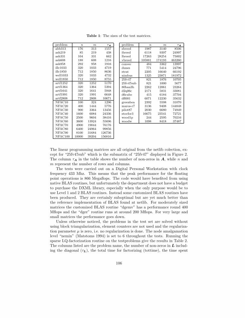
Table 1: The sizes of the test matrices.

problem n m τAabb313 176 313 1557ash219 85 219 438ash331 104 331 662ash608 188 608 1216ash958 292 958 1916illc1033 320 1033 4719illc1850 712 1850 8636well1033 320 1033 4732well1850 712 1850 8755artf1252 320 1252 5170artf1364 320 1364 5394artf1641 320 1641 5948artf1991 320 1991 6648artf2808 712 2808 10671NFAC10 100 324 1296NFAC20 400 1444 5776NFAC30 900 3364 13456NFAC40 1600 6084 24336NFAC50 2500 9604 38416NFAC60 3600 13924 55696NFAC70 4900 19044 76176NFAC80 6400 24964 99856NFAC90 8100 31684 126736NFAC100 10000 39204 156816

problem n m τAsbreed 1987 3140 8506ibreed 6118 9397 24997lbreed 17263 28254 75002vbreed 105881 174193 463260convec 484 3362 13997dunes 771 5414 24796strat 2205 16640 66192nimbus 1325 23871 18197225fv47 821 1876 1070525fv47sub 821 1000 567780bau3b 2262 12061 23264d2q06c 2171 5831 33081d6cube 415 6184 37704dfl001 6071 12230 35632greenbea 2392 5598 31070maros-r7 3136 9408 144848pilot87 2030 6680 74949stocfor3 16675 23541 72721wood1p 244 2595 70216woodw 1098 8418 37487

The linear programming matrices are all original from the netlib colection, ex-cept for “25fv47sub” which is the submatrix of “25fv47” displayed in Figure 2.The column τA in the table shows the number of non-zeros in A, while n andm represent the number of rows and columns.

The tests were carried out on a Digital Personal Workstation with clockfrequency 433 Mhz. This means that the peak performance for the floatingpoint operations is 866 Megaflops. The code would have benefited from usingnative BLAS routines, but unfortunately the department does not have a budgetto purchase the DXML library, especially when the only purpose would be touse Level 1 and 2 BLAS routines. Instead some customized BLAS routines havebeen produced. They are certainly suboptimal but are yet much better thanthe reference implementation of BLAS found at netlib. For moderately sizedmatrices the customized BLAS routine “dgemv” has a performance round 400Mflops and the “dger” routine runs at around 200 Mflops. For very large andsmall matrices the performance goes down.

Unless otherwise noticed, the problems in the test set are solved withoutusing block triangularization, element counters are not used and the regulariza-tion parameter µ is zero, i.e. no regularization is done. The node amalgamationlevel “nemin” (Matstoms 1994) is set to 6 throughout the tests. Running thesparse LQ-factorization routine on the testproblems give the results in Table 2.The columns listed are the problem name, the number of non-zeros in L includ-ing the diagonal (τL), the total time for factorizing (tottime), the time spent

106

Table 2: Results for the sparse LQ factorization routine of the software package.

Times are given in seconds.

problem τL tottime mindeg etree symb fact flop Mflopsabb313 1590 0.0528 0.0293 0.000977 0.00195 0.0205 90730 4.4ash219 531 0.00293 0.000977 0 0.000978 0.000978 49988 51.1ash331 780 0.00489 0.000977 0.000978 0.000977 0.00195 100348 51.3ash608 1673 0.00978 0.00293 0.000977 0.000978 0.00489 241855 49.5ash958 2602 0.0137 0.00391 0.00195 0.00195 0.00587 367767 62.7illc1033 2746 0.0254 0.0108 0.00293 0.00391 0.00782 519965 66.5illc1850 8007 0.0538 0.0225 0.00586 0.00489 0.0205 1457995 71.0well1033 2736 0.0235 0.00978 0.00293 0.00293 0.00782 526124 67.3well1850 8182 0.0527 0.0205 0.00585 0.00585 0.0205 1471885 71.8artf1252 3913 0.0361 0.0146 0.00293 0.0039 0.0146 1349633 92.2artf1364 4336 0.0459 0.0156 0.0039 0.0039 0.0224 2615946 116.6artf1641 5626 0.0566 0.0176 0.0039 0.00585 0.0293 3929304 134.3artf1991 10334 0.0898 0.0176 0.00585 0.00585 0.0605 9840935 162.7artf2808 21252 0.168 0.0371 0.0107 0.0127 0.107 16731221 155.9NFAC10 968 0.00488 0.00195 0 0.000976 0.00195 140220 71.9NFAC20 6893 0.0312 0.00585 0.0039 0.00488 0.0166 1528353 92.2NFAC30 20927 0.0888 0.0156 0.00976 0.0127 0.0507 5694709 112.3NFAC40 48411 0.2 0.0283 0.0195 0.0264 0.126 15814163 125.5NFAC50 78431 0.312 0.0459 0.0303 0.042 0.194 23086695 118.8NFAC60 152562 0.651 0.0684 0.0518 0.0762 0.455 57949405 127.5NFAC70 217911 0.9 0.0958 0.0723 0.114 0.618 82463769 133.5NFAC80 327007 1.43 0.126 0.101 0.159 1.05 137250314 131.0NFAC90 427475 1.85 0.167 0.133 0.208 1.34 177135369 132.3NFAC100 556590 2.66 0.209 0.174 0.274 2 258043905 128.9sbreed 14267 0.112 0.0381 0.0108 0.0088 0.0547 4249198 77.6ibreed 63929 0.533 0.132 0.0371 0.0342 0.329 30917810 93.8lbreed 160273 2.76 0.649 0.117 0.104 1.89 191280397 101.0vbreed 1207025 57.7 9.12 1.09 0.874 46.6 3207990256 68.8convec 16984 0.121 0.0186 0.00978 0.0108 0.0821 13145732 160.1dunes 29476 0.198 0.0342 0.0156 0.0196 0.129 19928592 154.7strat 116969 0.912 0.0907 0.0517 0.0683 0.701 110192147 157.2nimbus 141591 4.75 0.286 0.113 0.119 4.23 595085845 140.625fv47 36660 0.205 0.04 0.0117 0.0166 0.137 17445610 127.625fv47sub 19760 0.0674 0.0176 0.00586 0.00976 0.0342 3219607 94.280bau3b 45432 0.546 0.087 0.0264 0.0293 0.404 56505734 140.0d2q06c 185986 2.41 0.079 0.0449 0.0878 2.2 280828226 127.5d6cube 54459 6.86 0.161 0.0293 0.0361 6.63 530942222 80.1dfl001 1674660 109 0.501 0.274 0.686 108 8121177041 75.4greenbea 83972 0.599 0.131 0.039 0.0459 0.383 48650015 126.9maros-r7 1173609 38.3 0.648 0.214 0.461 37 3109901079 84.1pilot87 430050 16.4 0.452 0.0978 0.191 15.6 1526715428 97.8stocfor3 240810 0.889 0.269 0.106 0.12 0.395 22229647 56.3wood1p 19919 1.59 0.265 0.0352 0.0293 1.26 98066045 77.9woodw 50453 0.729 0.22 0.0341 0.0371 0.437 73078343 167.2

107

Table 3: The top of the execution profile when solving the linear programming prob-

lem “25fv47”.

% cumulative self self total

time seconds seconds calls ms/call ms/call name

16.4 1.87 1.87 1746 1.07 1.13 spfDowndate [8]

11.0 3.13 1.26 dger_ [9]

8.3 4.08 0.95 dgemv_ [14]

7.9 4.99 0.91 958 0.95 1.01 spfUpdate [13]

5.5 5.62 0.63 437 1.45 1.49 spfForsub [15]

5.1 6.21 0.59 dcopy_ [17]

4.7 6.75 0.54 71 7.63 16.25 spLQ [10]

4.3 7.24 0.49 116582 0.00 0.00 wstEliminateRow [18]

4.1 7.71 0.47 dnrm2_ [19]

4.0 8.17 0.46 71 6.45 14.38 rowamd [12]

3.6 8.58 0.41 26168 0.02 0.02 wspLQ [20]

2.5 8.87 0.29 437 0.66 0.70 spfBacksub [24]

2.0 9.10 0.23 336566 0.00 0.00 wstComprRowFindDiss [26]

1.8 9.31 0.21 213 0.99 0.99 wstFromMat [27]

1.6 9.49 0.18 409 0.44 0.44 spmxMVtrans [29]

1.5 9.66 0.17 330 0.51 0.51 spmxMV [30]

1.2 9.80 0.14 433543 0.00 0.00 spfEnhanceCol [32]

1.1 9.93 0.13 39732 0.00 0.00 quicksort [28]

in the approximate minimum degree routine (mindeg), the time spent findingthe elimination tree and doing the post-ordering (etree), the amount of timeused for the symbolic factorization (symb), the time spent in the multifrontalalgorithm (fact), the number of floating point operations used (flop) and finallythe Megaflops rate for the multifrontal code (Mflops).

Table 2 will be the reference point as we go on. First let us investigatethe updating and downdating routines. Using the updating routine to find thesparse factor L and beginning with an empty matrix gives the results in Table 4.The time taken for the approximate minimum degree algorithm and for findingthe elimination tree have been bundled together in the “analyse” column. Theelimination tree calculation is done just to get some idea of the number of non-zeros in L. Since the updating routine also builds up the structure of L, thesymbolic factorization is not needed. This is certainly not how the updatingroutine should be used, but it gives some information on how well the chosenupdating strategy works. On some very small problems it is actually competitiveto the multifrontal algorithm, considering total time. In general though, theflop count is excessive, compared to the multifrontal method, giving a hopelessdisadvantage. To get a better understanding of the performance of the updatingand downdating schemes, the netlib linear programming problem “25fv47” issolved with the code described in Edlund et al. (1999). The top of the profile forthe executed program is shown in Table 3. It was required to solve 437 systemsto find the solution. Out of those 71 were solved with refactorization using themultifrontal LQ algorithm and 233 solves were completed using updating anddowndating of the sparse factor L. The remaining 133 solves (including some

108

Table 4: Results for the updating routine of the software package when used as a tool

for finding L from scratch. Times are given in seconds.

problem τL tottime analyse fact flop Mflopsabb313 1590 0.0518 0.0391 0.0127 457589 36.0ash219 531 0.00489 0.00195 0.00293 96305 32.8ash331 780 0.00684 0.000977 0.00587 174817 29.8ash608 1673 0.0156 0.00391 0.0117 384113 32.7ash958 2602 0.0411 0.00586 0.0352 1385429 39.4illc1033 2744 0.0313 0.0147 0.0166 597063 35.9illc1850 7818 0.104 0.0313 0.0723 3219384 44.5well1033 2721 0.0303 0.0127 0.0176 675542 38.4well1850 7817 0.0811 0.0264 0.0547 2334088 42.6artf1252 3910 0.0566 0.0176 0.039 1647451 42.2artf1364 4333 0.0917 0.0205 0.0712 3442211 48.3artf1641 5623 0.152 0.0224 0.13 6636098 51.1artf1991 10108 0.381 0.0234 0.358 19709174 55.0artf2808 21212 1.02 0.0468 0.974 53619362 55.1NFAC10 968 0.00879 0.00195 0.00684 217830 31.9NFAC20 6893 0.17 0.0107 0.159 7960019 50.0NFAC30 20927 0.726 0.0264 0.7 37861421 54.1NFAC40 48411 3.26 0.0498 3.21 181201282 56.4NFAC50 78365 5.58 0.079 5.5 298354847 54.3NFAC60 151597 12.7 0.132 12.5 701016525 55.9NFAC70 216178 19.2 0.167 19 1043568355 54.9NFAC80 320172 34.5 0.225 34.3 1847522016 53.9NFAC90 421668 73.8 0.295 73.5 4040659706 54.9NFAC100 532575 63.2 0.382 62.8 3341630739 53.2sbreed 14267 0.153 0.0478 0.105 5427022 51.5ibreed 63929 1.76 0.165 1.59 87903994 55.2lbreed 160273 13.3 0.761 12.5 708515022 56.7vbreed 1197799 687 9.44 677 29803224061 44.0convec 12667 0.654 0.0273 0.627 34353269 54.8dunes 29475 3.6 0.0508 3.55 205026214 57.8strat 116730 34.5 0.146 34.3 1980346628 57.7nimbus 141591 116 0.378 116 6893717647 59.625fv47 36556 0.725 0.041 0.684 36182149 52.925fv47sub 17504 0.113 0.0342 0.0792 3600542 45.580bau3b 45432 3.37 0.101 3.27 185876221 56.9d2q06c 185957 15.8 0.119 15.7 888432615 56.6d6cube 54147 7.71 0.18 7.53 429960145 57.1dfl001 1674456 688 0.758 687 28513256737 41.5greenbea 83724 1.98 0.158 1.82 99466711 54.7maros-r7 1173609 305 0.848 304 13315389065 43.8pilot87 430044 99.5 0.542 98.9 4666869553 47.2stocfor3 240652 2.15 0.319 1.83 87580858 47.9wood1p 19919 1.97 0.266 1.71 97630707 57.2woodw 50453 6.82 0.243 6.57 380140108 57.8

109

iterative refinement steps) could be done without changing L. From Table 3we see that most of the total time is spent in the downdating and updatingroutines “spfDowndate” and “spfUpdate”, and in the BLAS routines “dger”and “dgemv”. The average times required for doing an update and a downdateare 1.01 ms and 1.13 ms respectively. This should be compared to the averagetimes for doing forward substitution of L and backward substitution of LT

which are 1.49 ms and 0.70 ms respectively. The conclusion is that the timerequired for a single update or downdate is comparable to the time required fora single forward or backward substitution. This behaviour has been observedalso for other linear programming problems.

Table 5 gives the results when block triangularization and element countersare in use. The additional column “blocktri” gives the time taken for findingthe maximum matching and the Dulmage-Mendelsohn decomposition.

When the approximate minimum degree algorithm of the software package isreplaced by “colamd” by Davis & Larimore (Larimore 1998), we get the resultsin Table 6. Comparing to Table 2, we see that their implementation seems tobe a little better even though the difference is not very pronounced.

The multifrontal factorization routine is also compared to the QR27 codedescribed in Matstoms (1994). In these tests, the routine MA27 of the Harwelllibrary is called to find the minimum degree reordering, since that is the routinepackaged with QR27. Despite several attempts it turned out to be very difficultto call QR27 with a customized reordering. In Table 7 the two multifrontalimplementations are compared. There seems to be a slight advantage for QR27,even though the difference is small, with the exception of “vbreed” and “dfl001”,where the difference is significant.

8 Conclusions and Discussion

The tests above seem to indicate that the software package indeed is adequatefor its purpose. The updating and downdating routines work quite well, thoughit is difficult to make comparisons since no alternative is available. The use of el-ement counters in the symbolic factorization is a simple and fast solution to howto find the correct prediction of non-zero fill after the block triangularization.This gives the best prediction of the number of non-zeros in L, as described inColeman et al. (1986). However, this is an issue only if the matrix AA does notpossess the strong Hall property. And even if that condition is fulfilled, a matrixwith rank lower than n may cause trouble. If a diagonal entry of L happensto be so small that the only viable numerical interpretation is that it is zero,it is required that all the below diagonal elements are zero, to be able to finda “basic” solution to a consistent system. Therefore the below diagonal entrieshave to be rotated into the rest of the matrix. If this happens inside a squarediagonal block, the structure of that column will most likely contaminate thenon-zero structure of the matrix outside the block column. The effect of thiscontamination is NOT considered in the sparsity analysis when block triangu-larization is used. If neither block triangularization nor element counters are

110

Table 5: Results when block triangularization is used. Times are given is seconds.

problem τL tottime blocktri mindeg etree symb fact flop Mflopsabb313 1590 0.081 0.0185 0.0205 0.000976 0.000975 0.04 90235 2.3ash219 542 0.0039 0.000975 0.000976 0 0.000975 0.000976 54876 56.2ash331 748 0.00488 0 0.00195 0 0.000975 0.00195 90336 46.3ash608 1658 0.0195 0 0.00293 0.00196 0.000977 0.0137 249485 18.2ash958 2557 0.0146 0.000976 0.00391 0.00195 0.00195 0.00586 360152 61.5illc1033 2695 0.0264 0.00195 0.0107 0.00293 0.00293 0.00781 434366 55.6illc1850 7760 0.0605 0.00293 0.0244 0.00684 0.00586 0.0205 1450565 70.7well1033 2674 0.0234 0.000976 0.00781 0.00391 0.00293 0.00781 442434 56.6well1850 7791 0.0566 0.00293 0.0225 0.00586 0.00586 0.0195 1382147 70.8artf1252 3878 0.0361 0.00195 0.0127 0.00293 0.00391 0.0146 1474372 100.6artf1364 4249 0.043 0.00195 0.0146 0.00293 0.00391 0.0195 2071209 106.0artf1641 5555 0.0547 0.000977 0.0166 0.00488 0.00391 0.0283 3647370 128.8artf1991 9799 0.085 0.00195 0.0176 0.00586 0.00684 0.0527 8505597 161.3artf2808 23260 0.209 0.00391 0.0391 0.0108 0.0127 0.143 22501038 157.7NFAC10 976 0.00587 0 0.00195 0 0.000978 0.00293 166724 56.8NFAC20 6725 0.0352 0.00195 0.00782 0.00391 0.00489 0.0166 1591273 95.8NFAC30 21505 0.0997 0.00293 0.0176 0.00977 0.0137 0.0557 6375763 114.4NFAC40 52819 0.229 0.00684 0.0303 0.0196 0.0303 0.142 17765492 125.3NFAC50 89187 0.376 0.0107 0.0488 0.0322 0.0488 0.235 28912196 123.0NFAC60 144255 0.611 0.0146 0.0732 0.0507 0.078 0.394 49738238 126.1NFAC70 211775 0.897 0.0215 0.104 0.0713 0.113 0.587 72190799 122.9NFAC80 317855 1.39 0.0283 0.134 0.0996 0.166 0.959 126925433 132.3NFAC90 437749 2 0.0381 0.181 0.136 0.231 1.41 179691353 127.4NFAC100 532808 2.45 0.0459 0.235 0.177 0.285 1.7 209581728 122.9sbreed 14197 0.122 0.00489 0.0411 0.0117 0.00978 0.0547 4120890 75.3ibreed 65753 0.59 0.0137 0.143 0.0371 0.0371 0.359 33758417 94.0lbreed 162688 3.07 0.0507 0.809 0.12 0.11 1.98 192604215 97.5vbreed 1213945 60.1 0.441 9.39 1.15 0.911 48.2 3351704837 69.6convec 17450 0.147 0.00391 0.0195 0.0117 0.0117 0.0996 13958112 140.1dunes 29332 0.219 0.00489 0.0362 0.0166 0.0235 0.138 20071509 145.6strat 104569 0.788 0.0195 0.1 0.0546 0.0644 0.549 90601013 165.1nimbus 143381 5.25 0.0381 0.289 0.105 0.131 4.68 625949611 133.625fv47 33884 0.177 0.00683 0.0293 0.0117 0.0156 0.113 14815018 130.925fv47sub 15018 0.0547 0.00586 0.0117 0.00488 0.00683 0.0254 2176309 85.780bau3b 43982 0.537 0.00976 0.0713 0.0244 0.0303 0.401 55295794 137.8d2q06c 195255 2.56 0.00782 0.0821 0.045 0.0831 2.34 297999829 127.3d6cube 53737 4.07 0.0156 0.152 0.0284 0.0381 3.84 392188300 102.1dfl001 1605478 89.4 0.0205 0.463 0.272 0.66 88 7245987595 82.4greenbea 84327 0.561 0.0224 0.118 0.038 0.0459 0.337 44304475 131.6maros-r7 1170970 32.3 0.0264 0.634 0.211 0.467 31 3084982477 99.7pilot87 437111 16.9 0.0137 0.502 0.101 0.187 16.1 1678195866 104.4stocfor3 218667 0.836 0.0293 0.227 0.0997 0.106 0.374 18068992 48.3wood1p 19802 1.54 0.0127 0.223 0.0449 0.0322 1.22 95735073 78.2woodw 48951 0.7 0.0107 0.204 0.0332 0.0381 0.413 66286453 160.3

111

Table 6: Results when the routine “colamd” is used for the minimum degree calcula-

tions.

problem τL tottime colamd etree symb fact flop Mflopsabb313 1597 0.0615 0.000975 0.0224 0.000976 0.0371 92737 2.5ash219 514 0.00293 0 0.000976 0 0.00195 45826 23.5ash331 744 0.0039 0 0.000975 0.000976 0.00195 93782 48.1ash608 1589 0.00878 0.00195 0.000975 0.00195 0.0039 224605 57.5ash958 2503 0.0127 0.00195 0.00293 0.00195 0.00585 358554 61.2illc1033 2967 0.0234 0.00975 0.00293 0.00293 0.0078 572629 73.4illc1850 8657 0.0527 0.0205 0.00585 0.00683 0.0195 1521664 78.0well1033 2997 0.0205 0.00585 0.0039 0.00293 0.0078 595582 76.3well1850 8886 0.0488 0.0166 0.00683 0.00488 0.0205 1573621 76.8artf1252 4503 0.0361 0.0127 0.00293 0.0039 0.0166 1777498 107.2artf1364 4634 0.0419 0.0146 0.0039 0.0039 0.0195 2134504 109.4artf1641 6094 0.0546 0.0166 0.00488 0.00488 0.0283 3842237 135.8artf1991 9535 0.0761 0.0156 0.00683 0.00585 0.0478 7277026 152.2artf2808 22517 0.174 0.0312 0.0107 0.0127 0.119 18736357 157.3NFAC10 889 0.00488 0.000977 0.000976 0.000977 0.00195 108840 55.7NFAC20 6236 0.0303 0.00879 0.00391 0.00391 0.0137 1115074 81.6NFAC30 23091 0.105 0.0303 0.00879 0.0107 0.0557 6234288 112.0NFAC40 46484 0.193 0.0469 0.0166 0.0234 0.106 12222175 114.8NFAC50 78127 0.317 0.0723 0.0284 0.0381 0.178 20242973 113.8NFAC60 124372 0.499 0.103 0.042 0.0625 0.292 33155078 113.7NFAC70 174033 0.678 0.136 0.0556 0.0839 0.403 46561998 115.5NFAC80 236367 0.905 0.171 0.0771 0.116 0.541 64496135 119.3NFAC90 310461 1.19 0.222 0.102 0.157 0.711 86626933 121.8NFAC100 393025 1.51 0.281 0.133 0.196 0.904 112331004 124.3sbreed 14248 0.0985 0.0254 0.0107 0.00878 0.0537 4083184 76.1ibreed 64618 0.517 0.0868 0.0341 0.0351 0.361 33074568 91.6lbreed 154125 2.15 0.431 0.113 0.109 1.49 157583024 105.6vbreed 1189600 49.7 4.47 1.06 0.859 43.3 3094546476 71.4convec 14401 0.089 0.0127 0.0088 0.00978 0.0577 8500266 147.4dunes 26959 0.177 0.0371 0.0156 0.0166 0.107 16506153 153.8strat 101930 0.699 0.102 0.0498 0.0576 0.489 81228292 166.1nimbus 134236 4.76 0.539 0.0958 0.102 4.03 590051873 146.525fv47 39498 0.176 0.0205 0.0127 0.0176 0.125 18318807 146.625fv47sub 18094 0.0508 0.0107 0.00684 0.00781 0.0254 2178218 85.880bau3b 44263 0.518 0.0518 0.0264 0.0283 0.411 55914840 136.0d2q06c 175041 1.97 0.0528 0.043 0.0733 1.8 236022439 131.1d6cube 53285 5.38 0.0645 0.0283 0.0332 5.25 438297603 83.5dfl001 1544706 138 0.314 0.263 0.628 137 8561600824 62.7greenbea 79425 2.58 0.797 0.18 0.182 1.42 34238226 24.0maros-r7 853785 17.5 2.54 0.187 0.609 14.2 1546393742 109.1pilot87 422518 25 0.4 0.103 0.177 24.3 1818476933 74.8stocfor3 234325 0.748 0.166 0.11 0.111 0.36 18912805 52.6wood1p 24266 1.94 0.108 0.0488 0.038 1.74 122650692 70.5woodw 45438 0.574 0.186 0.0332 0.0352 0.32 51364281 160.4

112

Table 7: A comparison with QR27.

spLQ QR27problem τL fact flop Mflops fact flop Mflopsabb313 1601 0.0538 94449 1.8 0.039 103082 2.6ash219 510 0.00195 45991 23.5 0.000976 46173 47.3ash331 774 0.00195 102108 52.2 0.00195 89196 45.7ash608 1637 0.0039 237578 60.9 0.0039 224180 57.5ash958 2612 0.00585 383817 65.6 0.0078 348558 44.7illc1033 2583 0.00878 479016 54.6 0.00683 334575 49.0illc1850 7478 0.0224 1426084 63.6 0.0195 1228562 63.0well1033 2589 0.00878 450785 51.3 0.0078 326229 41.8well1850 7492 0.0293 1289889 44.1 0.0195 1149422 58.9artf1252 3658 0.0146 1413582 96.6 0.0146 1103493 75.4artf1364 4160 0.0195 2115410 108.4 0.0176 1564056 89.1artf1641 5631 0.0312 4022041 128.7 0.0293 3306610 112.9artf1991 9943 0.0605 9668045 159.7 0.0596 8827432 148.2artf2808 20521 0.107 15988272 148.8 0.0986 14020117 142.1NFAC10 921 0.00195 134136 68.7 0.00293 111331 38.0NFAC20 6033 0.0137 1076886 78.8 0.0137 888658 65.0NFAC30 17973 0.04 3190504 79.7 0.042 3227253 76.9NFAC40 38438 0.0772 7276232 94.2 0.0889 7502141 84.4NFAC50 65249 0.137 13008970 95.1 0.155 13239148 85.2NFAC60 108907 0.225 23167459 102.8 0.253 23859454 94.2NFAC70 141817 0.299 29718170 99.4 0.332 30548974 92.1NFAC80 228639 0.506 56511552 111.7 0.555 57867901 104.3NFAC90 258867 0.563 59675798 106.0 0.621 61178833 98.6NFAC100 404472 0.986 115609070 117.2 1.12 117855197 105.3sbreed 14087 0.0499 3476663 69.7 0.0508 3478092 68.5ibreed 67103 0.386 35566317 92.1 0.271 26203413 96.5lbreed 154693 1.5 160391466 106.8 0.984 112646809 114.5vbreed 1242922 50.2 3580934599 71.3 19.6 1792321842 91.2convec 15908 0.0694 10431688 150.4 0.0664 10019596 150.9dunes 27448 0.115 18054953 156.7 0.109 16098269 147.2strat 107673 0.531 84916889 159.8 0.478 77537674 162.2nimbus 144592 4.85 609070944 125.7 4.4 585157611 132.925fv47 35054 0.12 16372865 136.4 0.12 15818659 131.725fv47sub 17332 0.0283 2257123 79.8 0.0303 2242796 74.180bau3b 42565 0.418 49511048 118.6 0.326 44187983 135.7d2q06c 159157 1.68 211741837 126.2 1.61 189532712 117.5d6cube 54711 7.23 492235748 68.1 7.2 475533786 66.0dfl001 1651196 130 7997202595 61.5 40.1 7859146164 195.9greenbea 88112 0.445 48467484 109.0 0.378 45483674 120.2maros-r7 1257330 60.8 3515519814 57.8 40.3 3570749043 88.5pilot87 412997 16 1488755711 93.0 17 1937662444 113.7stocfor3 222811 0.352 17478766 49.7 0.449 18568657 41.4wood1p 18326 0.524 49244606 93.9 0.31 44481898 143.7woodw 49000 0.428 64848187 151.6 0.374 58204295 155.5

113

considered the opposite is true, thus it is assumed that ALL columns contam-inate the rest of the matrix. These facts are important to keep in mind whenusing block triangularization to solve systems. Most likely it is beneficial to useit, but under certain circumstances there may be substantial additional fill-in.However, if the matrix is known a priori to have rank n there is no danger. Andeven if the matrix has lower rank, the updating facility of the software packagemakes it possible to handle it. To do this properly though, a rank revealingfacility would need to be included, but that is outside the scope of what thissoftware package is aimed for.

The comparison with the approximate minimum degree code “colamd” re-vealed that the code in spLQ is not quite up to par. This is strange sincethe algorithms are more or less identical. In fact looking at τL and the timespent in the minimum degree code, the difference is negligible. It is in the“flop” and “tottime” columns that the difference is obvious. It seems as though“colamd” does a better job in minimizing the operation count for LQ or QRfactorizations. Perhaps this could be a result of the choice of method to cal-culate initial degrees, but the code in spLQ suffered from even worse resultswhen MATLAB style degree approximations were used initially. Under thesecircumstances perhaps “colamd” should be used instead. However, this was notan option in 1996 when the first version of the code in spLQ was produced. Ifblock triangularization is considered, the code in spLQ is the only option.

The multifrontal factorization code in spLQ cannot however be exchangedfor QR27 since it is “hardwired” with the dynamic representation of L and withthe representation of the column subset AA. The small difference there is, inthe computation time, may be erased by including the “restricted factorization”feature of Matstoms (1994).

Another thing needed to be improved is the handling of dense columns. Asingle dense column in AA makes L completely filled with non-zeros. Thismay be handled by disregarding the dense column in the factorization phaseand instead determine its impact on the solution with Schur-complements. Ifq columns are dense this involves solving the sparse system with q + 1 righthand sides and then finding the solution to a dense unsymmetric q × q systemto figure out how to combine the solutions for each right hand side.

The element counters introduced in section 5 might very well be applied inthe approximate minimum degree code as an estimate of the operation count forthe Householder reflections. This would give an efficient and highly competitivereordering code that is specially designed for LQ or QR factorization. Somepossible strategies could be to

1. abandon degrees, and just consider element counter sums for choosingvariables,

2. use approximate degrees, and use the element counters sums to resolveties, or

3. use the operation count for the Householder reflection to choose variables.

114

Note that the element counter sum above refers to the count a new elementwould get as a variable is eliminated. These quantities are easily calculatedby traversing the adjacency lists of the variables and summing up the elementcounters. The operation count for the Householder reflection in alternative 3above is easy to estimate by multiplying the degrees and the element countersums associated with the variables. The biggest “problem” is that we cannothave both “aggressive” element absorption and element counters at the sametime. Elements with equal adjacency lists may be absorbed though. In thatcase the element counters are just added. Alternatively it may be a good ideato disregard this restriction doing aggressive element absorption anyway, andjust add the count of the absorbed element to the absorbing elements counter.Alternative 1 above is probably the fastest, but anyone looking for higher qualityreorderings should probably choose 2 or 3.

Acknowledgements

The author would like to thank Hans Bruun Nielsen and John Reid for theirhelpful advises and Pontus Matstoms for generously providing the test problemsand the source code for QR27.

References

Amestoy, P., Davis, T. A. & Duff, I. S. (1996), ‘An approximate minimum degreeordering algorithm’, SIAM J. Matrix Anal. Appl. 17(4), 886–905.

Coleman, T. F., Edenbrandt, A. & Gilbert, J. R. (1986), ‘Predicting fill forsparse orthogonal factorization’, J. Assoc. Comput. Mach. 33(3), 517–532.

Duff, I. S. (1981), ‘On algorithms for obtaining a maximum traversal’, ACMTrans. Math. Software 7(3), 315–330.

Duff, I. S., Erisman, A. M. & Reid, J. K. (1986), Direct Methods for SparseMatrices, Oxford University Press.

Duff, I. S. & Wiberg, T. (1988), ‘Remarks on implementations of O(n1/2τ)assignment algorithms’, ACM Trans. Math. Software 14(3), 267–287.

Edlund, O., Madsen, K. & Nielsen, H. B. (1999), A piecewise quadratic approachfor solving sparse linear programming problems. To be submitted.

George, A. & Liu, J. W. H. (1989), ‘The evolution of the minimum degreeordering algorithm’, SIAM Rev. 31(1), 1–19.

Gilbert, J. R., Moler, C. & Schreiber, R. (1992), ‘Sparse matrices in Matlab:Design and implementation’, SIAM J. Matrix Anal. Appl. 13(1), 609–629.

Golub, G. H. & Van Loan, C. F. (1989), Matrix Computations, second edn, TheJohns Hopkins University Press.

115

Hopcroft, J. E. & Karp, R. M. (1973), ‘An n5/2 algorithm for maximum match-ings in bipartite graphs’, SIAM J. Comput. 2, 225–231.

Larimore, S. I. (1998), An approximate minimum degree column ordering algo-rithm, CISE Tech Report TR-98-016, Dept. of Computer and InformationScience and Engineering, University of Florida, Gainesville, FL. MS Thesis.

Madsen, K. & Nielsen, H. B. (1990), ‘Finite algorithms for robust linear regres-sion’, BIT 30, 333–356.

Madsen, K. & Nielsen, H. B. (1993), ‘A finite smoothing algorithm for linear `1estimation’, SIAM J. Optimization 3(2), 223–235.

Madsen, K., Nielsen, H. B. & Pınar, M. C. (1996), ‘A new finite continuationalgorithm for linear programming’, SIAM J. Optimization 6(3), 600–616.

Matstoms, P. (1994), Sparse QR Factorization with Applications to LinearLeast Squares Problems, Ph.D. dissertation, Department of Mathematics,Linkoping University, S-581 83 Linkoping, Sweden.

Matstoms, P. (1997), ‘Sparse linear least squares problems in optimization’,Comput. Optim. Appl. 7(1), 89–110.

Nielsen, H. B. (1990), AAFAC, a package of Fortran77 subprograms for solvingATAx = c, Technical Report NI-90-01, Institute for Numerical Analysis,Technical University of Denmark, Lyngby 2800, Denmark.

Pınar, M. C. (1997), ‘Piecewise-linear pathways to the optimal set in linearprogramming’, Journal of Optimization Theory and Applications 93, 619–634.

Pothen, A. & Fan, C.-J. (1990), ‘Computing the block triangular form of asparse matrix’, ACM Trans. Math. Software 16(4), 303–324.

116