0

Overreacting to a History of Underreaction?

Jonathan A. Milian

Florida International University School of Accounting

11200 S.W. 8th St. Miami, FL 33199

jonathan.milian@fiu.edu

March 2013

ABSTRACT

Prior research has documented a long history of positive autocorrelation in firms’ earnings announcement news. This is one of the main features of the post-earnings announcement drift phenomenon and is typically attributed to investors’ underreaction to earnings news. I document that this autocorrelation has become significantly negative for firms with active exchange-traded options. For these easy-to-arbitrage firms, the firms in the highest decile of prior earnings announcement abnormal return (prior earnings surprise), on average, underperform the firms in the lowest decile by 1.29% (0.73%) at their next earnings announcement. Additional analyses are consistent with investors learning about post-earnings announcement drift and overcompensating. For example, I find that, in recent years, stock returns are more extreme in response to extreme earnings surprises, and that investors are positioning themselves immediately prior to the next earnings announcement in anticipation of PEAD (i.e., buying shares or call options of past earnings announcement winners and selling-short or buying put options of past earnings announcement losers). It seems that due to their well-documented history of apparently underreacting to earnings news, investors are now overreacting to earnings announcement news. This paper shows that attempts to exploit a popular trading strategy based on relative valuation can significantly reverse the previously documented pattern.

1

1. INTRODUCTION

Grossman and Stiglitz (1980) note that only through costly information search and trading by

arbitrageurs are security prices driven towards fundamental value, and Lee (2001) discusses

market efficiency as a process and a journey, one in which financial researchers can help lead the

market towards greater efficiency. While on this journey, financial researchers have documented

an extensive set of cross-sectional stock return predictors or anomalies (Green et al. 2013). In

his review of anomalies, Schwert (2003) argues that increased arbitrage activity should cast

doubt on whether these anomalies can persist. Consistent with a market that becomes more

efficient over time, recent research has found that many of the most well-known anomalies no

longer present profitable trading opportunities (e.g., Chordia et al. 2013; Green et al. 2011;

Richardson et al. 2010). While this recent research is consistent with the notion of an

increasingly efficient market in which arbitrageurs exploit opportunities to the point that the

opportunities are no longer profitable, it is not clear that attempts to profit from a well-known

cross-sectional anomaly always drives prices to fundamental values.

Attempts to exploit well-known cross-sectional anomalies do not necessarily drive prices to

fundamental values because these trading strategies are based on relative values rather than

absolute or fundamental values. As these trading strategies are not based on estimates of

fundamental value, arbitrageurs relying solely on these strategies never know the extent of the

mispricing, if any. This inherent uncertainty regarding the magnitude of the mispricing requires

the arbitrageurs to understand the price impact, if any, of other arbitrageurs using the same

strategy. Stein (2009) and Lundholm (2008) present theoretical models where some arbitrageurs

trade using relative value strategies without consideration for fundamental value. They show

that when this arbitrage activity becomes too aggressive, these arbitrageurs can cause the

2

opposite of the expected cross-sectional return pattern instead of eliminating the pattern.

Similarly, Lo (2004) argues that in an adaptive market, trading strategies will undergo cycles of

profit and loss depending on the magnitude of the profit opportunities and on the amount of

capital used by arbitrageurs in the trading strategies. From these theoretical models, I

hypothesize that the return pattern from a well-known cross-sectional anomaly can significantly

reverse over a nontrivial period of time due to an overcrowding of arbitrageurs in that trading

strategy.

To test my hypothesis, I examine one of the main features of the post-earnings announcement

drift (PEAD) phenomenon. Specifically, I examine the autocorrelation in earnings

announcement news for firms with active exchange-traded options. I select this setting because

it has several attractive features that increase the likelihood of it being an overcrowded trade.

First, the PEAD effect is one of the most well-known cross-sectional anomalies due to its long

and extensively documented history. Second, exploiting the effect is not viewed as particularly

risky because the most popular explanation for PEAD is that investors underreact to earnings

news. Third, I focus my analysis on firms with active exchange-traded options because the

strategy is easier to implement in these firms relative to firms without active options. Finally,

because the magnitude of the abnormal returns is large and the timing of those abnormal returns

is precise, this aspect of the PEAD effect is attractive to potential arbitrageurs (especially ones

using options) as they are after opportunities with the greatest amount of abnormal returns

possible per unit of time.

Consistent with my hypothesis, I find that instead of the expected positive autocorrelation in

firms’ earnings announcement news from the PEAD literature, there is a significantly negative

autocorrelation in firms’ earnings announcement news for firms with active options trading

3

during my 1996 – 2010 sample period. This significantly negative relation between firms’

current earnings announcement abnormal returns and their prior earnings announcement news is

of large economic significance, and is present regardless of whether the prior earnings news is

measured as the prior earnings surprise or as the abnormal stock return at the prior earnings

announcement. From 1996 - 2010, firms in the highest decile of prior earnings announcement

abnormal returns (prior earnings surprises), on average, significantly underperform firms in the

lowest decile by 1.29% (0.73%) over their next two-day earnings announcement window.

For firms with active options trading, prior earnings news remains a significantly negative

predictor of future earnings announcement abnormal returns even after controlling for various

variables that prior research has shown to predict future earnings announcement abnormal

returns. In fact, it is the second most powerful predictor of future earnings announcement

abnormal returns for firms with active options.1 This new negative relation is a more powerful

predictor than classic earnings announcement abnormal return predictors such as size (e.g.,

Freeman 1987; Chari et al. 1988; Ball and Kothari 1991), growth (La Porta et al. 1997), and

accruals (Sloan 1996). It is also a stronger predictor of earnings announcement abnormal returns

than newly discovered predictors from options data such as option spreads (Jin et al. 2012;

Atilgan 2012), option skews (Jin et al. 2012; Van Buskirk 2011), and O/S - option trading

volume relative to share volume (Johnson and So 2012; Roll et al. 2010).

I examine three possible explanations for the negative autocorrelation in earnings news, and

find some evidence consistent with each of them. First, I find that the stock price reactions to

earnings surprises are more extreme in recent years (2003Q3 – 2010). This is consistent with

investors learning from their past underreaction and overcompensating. Second, I find that

1 The most powerful predictor of the earnings announcement abnormal returns in my sample is the abnormal return in the days immediately prior to the earnings announcement (So and Wang 2011; Landsman et al. 2011; Aboody et al. 2013).

4

proxies of firm-specific investor sentiment are significantly higher (lower) immediately prior to

the next earnings announcements for firms that did well (poorly) at their previous earnings

announcement. This is consistent with investors overly positioning themselves in a manner

consistent with the expectation of the PEAD effect, and this excessive sentiment being corrected

when the earnings news is released, resulting in negative autocorrelation in firms’ earnings news.

Finally, I find that the autocorrelation in firms’ earnings surprises is still significantly positive,

but that after controlling for a firm’s prior earnings surprise, a firm’s prior earnings

announcement return is negatively associated with the firm’s next earnings surprise. This is

consistent with analysts overreacting to the other information in firms’ earnings announcements

that is unrelated to the earnings surprise, when they forecast next quarter’s earnings. Overall, the

evidence is consistent with investors learning about PEAD and trading more aggressively at both

the current earnings announcement and immediately prior to the next earnings announcement in

an effort to profit from PEAD.

The results that I document are of interest to both financial researchers and practitioners

alike. Consistent with the theoretical models of Stein (2009) and Lundholm (2008), I document

that the return pattern from a well-known cross-sectional anomaly can significantly reverse for

an extended period of time. These theoretical models and my results suggest that arbitrage

activity related to cross-sectional anomalies does not always drive prices towards fundamental

value. In fact, arbitrage activity can actually reverse the cross-sectional stock return pattern that

it intends to eliminate. This result should caution investors not to blindly follow relative value

trading strategies because the worst-case scenario is not that the strategy will not work (i.e., earn

zero excess returns), the worst-case scenario is that the strategy will consistently fail (i.e., earn

negative excess returns).

5

The rest of the paper is organized as follows. Section 2 discusses prior literature and

motivates the paper. Section 3 describes the data. Section 4 reports the main result. Section 5

examines potential explanations for the main result. Section 6 concludes.

2. LITERATURE REVIEW AND MOTIVATION

2.1 Elimination of Cross-sectional Anomalies

Over the past several decades, a large literature has developed documenting the ability of

various cross-sectional variables to predict future stock returns (Green et al. 2013). Explanations

for these phenomena generally relate to risk (e.g., Fama and French 1993), behavioral biases

(e.g., Lakonishok et al. 1994), transaction costs (e.g., Amihud and Mendelson 1986), or arbitrage

costs (e.g., Shleifer and Vishny 1997). To the extent that some of these cross-sectional variables

are unrelated to risk, reductions in transaction costs and increases in arbitrage activity should call

into question how long a variable’s predictive ability can persist (e.g., Schwert 2003).

Consistent with this argument, a new literature is developing that documents a reduction in

(or the elimination of) the stock return predictability due to some of these well-established

variables. For example, Chordia et al. (2013) find that the predictive ability of seven of the most

well-known cross-sectional predictors (i.e., firm size, book-to-market ratio, past twelve month

return, accruals, change in shares outstanding, idiosyncratic volatility, and standardized

unexpected earnings) are significantly weaker in recent years for liquid firms. They attribute this

decline in predictive ability to increased arbitrage activity (e.g., increases in hedge funds’ assets

under management and increases in short interest) and reduced transaction costs (e.g., decreases

in tick size and increases in trading volume).

6

Several other papers also use arguments involving investor learning, increased arbitrage

activity, and decreases in transaction costs to explain the reduction in (or the elimination of)

excess returns to various cross-sectional trading strategies. McLean and Pontiff (2012) examine

82 different anomalies and find that on average the post-publication abnormal returns decrease

by about 35%. Research specifically examining the two most popular accounting-based trading

strategies, PEAD and the accrual anomaly, suggest decreases much larger than 35%. Green et al.

(2011) find that abnormal returns to the accrual anomaly strategy have not been reliably positive

since 2001. Johnson and Schwartz (2000) find that abnormal returns to the PEAD strategy were

substantially eliminated during the 1991 – 1997 period for large firms, and Chordia et al. (2013)

find no evidence of PEAD in liquid stocks during the 1994 – 2011 period. Richardson et al.

(2010) find that, after transaction costs, returns to both the accrual anomaly and PEAD strategies

have attenuated in recent years. These papers are consistent with a market that becomes more

efficient over time, as it learns about and then reduces or eliminates profitable trading

opportunities.

However, it is not clear that attempting to eliminate these cross-sectional patterns in stock

returns is an attractive opportunity to an arbitrageur because a significant issue arises when

implementing a trading strategy to exploit one of these documented cross-sectional patterns. The

problem is that the trading strategies used to exploit these patterns involve buying and selling

stocks of firms in the extremes of a given variable’s distribution, meaning that the strategies are

relying on stocks’ relative values rather than absolute or fundamental values. Without an

estimate of a firm’s fundamental value, the arbitrageur has no idea as to the extent of the

mispricing, if any. Given that an arbitrageur solely using a cross-sectional trading strategy does

7

not consider the magnitude of the mispricing, they must also concern themselves with the price

impact that other arbitrageurs using the same strategy may have on stock prices.

Both Stein (2009) and Lundholm (2008) model a setting in which some arbitrageurs trade

using these relative value strategies without consideration for fundamental value. They show

that when arbitrage activity is too high, the arbitrageurs can push prices beyond the efficient

level, thereby causing the opposite of the expected return pattern rather than eliminating the

pattern. In other words, if arbitrage activity using a trading strategy is too high, it becomes

profitable to take the opposite positions. Lo (2004) also emphasizes that the number and size of

arbitrageurs can cause a previously profitable trading strategy to become unprofitable.

Two case studies in which arbitrage attempts (based on a cross-sectional pattern) went awry

are found in Stein (2009) and Khandani and Lo (2007). In both cases, it appears that too much

capital was invested in a particular trading strategy resulting in very poor returns for the

arbitrageurs. The case discussed in Stein (2009) involves an index rebalancing in late 2001.

Contrary to expectations and past rebalancings, a strategy that was long stocks to be upweighted

in the index and short stocks to be downweighted lost 6.18% on the day of the rebalance.

Similarly, Khandani and Lo (2007) show that returns to a short-term reversal strategy, which had

typically earned positive returns in the past, had a three-day return of -6.85% during the week of

August 6, 2007. While these two case studies are illustrative and interesting, they do not

document that excessive arbitrage activity can consistently reverse a previously documented

cross-sectional pattern, which is my interest.

The theoretical models of Stein (2009) and Lundholm (2008), the arguments in Lo (2004),

and these two case studies demonstrate the unintended impact that arbitrageurs can have on

market prices. I hypothesize that an overcrowding of arbitrageurs may be detectable in the time-

8

series of returns for an aspect of the PEAD strategy. I specifically focus on the PEAD strategy

and one particular aspect of it for reasons that I discuss next.

2.2 Post-earnings Announcement Drift

Ball and Brown (1968) first documented a phenomenon called post-earnings announcement

drift (PEAD).2 They show that prices continue to drift in the direction of the earnings news for a

period of time after the announcement. Interest in this anomaly resurged after Bernard and

Thomas (1989), who show that an implementable trading strategy based on PEAD (i.e., buying

stocks in the highest decile of unexpected earnings and shorting stocks in the lowest decile)

generates an 18% annualized return, during the quarter after the earnings announcement.

Knowledge of the PEAD phenomenon has been widely disseminated (e.g., there is a relatively

detailed discussion of it in the leading undergraduate textbook on investments Bodie et al. 2004).

The most popular explanation for the drift and the autocorrelation in earnings news is that

investors underreact to earnings information. 3 For instance, Fama (1998) refers to PEAD as “the

granddaddy of underreaction events.” Ball and Bartov (1996) find that investors underestimate

the magnitude of serial correlation in seasonally-differenced quarterly earnings by about 50%.4

Also inconsistent with a risk-based explanation, Bernard and Thomas (1989) find that a hedge

portfolio based on PEAD earned positive returns in 46 of 50 quarters and in all 13 years that they

examine.

Relative to other anomalies, PEAD’s long history, extensive documentation, wide

dissemination, and evidence of a non-risk explanation make it an interesting anomaly for

2 See Ball (1992), Bernard (1993), Kothari (2001), Richardson et al. (2010), and Taylor (2011) for literature reviews. 3 Other explanations generally involve risk, arbitrage costs, and/or transaction costs (e.g., Ball 1978; Ball et al. 1993; Sadka 2006; Garfinkel and Sokobin 2007; Mendenhall 2004; Bhushan 1994; and Ng et al. 2008). 4 Other papers on investors underestimation of the autocorrelation in seasonally-differenced quarterly earnings include: Rendleman, Jones, and Latane (1987), Bernard and Thomas (1990), and Soffer and Lys (1999).

9

arbitrageurs to pursue. However, for these same reasons concerns about a potentially

overcrowded trade also arise. Consistent with increased arbitrage activity reducing the abnormal

returns to the PEAD strategy, Johnson and Schwartz (2000), Richardson et al. (2010), and

Chordia et al. (2013) find that the strategy has not been significantly profitable in recent years.5

While these papers examine the abnormal returns in the weeks or months following the earnings

announcement, one key finding from the PEAD literature that these studies do not examine is

that a large proportion of the future abnormal returns occur at future earnings announcements,

especially at the next earnings announcement (Bernard and Thomas 1989; Freeman and Tse

1989). For example, Bernard and Thomas (1989) find that 40%, 29%, and 25% of the 60-day

drift occurs at the next earnings announcement for small, medium, and large firms, respectively.

I examine this aspect of PEAD because of its specificity as to when to expect the mispricing

to correct itself (which creates a more direct link between past and future earnings information)

and because a short return window reduces issues regarding the measurement of abnormal

returns.6 In addition to increasing the power of the empirical test, this setting is also relatively

more attractive to arbitrageurs as they are likely to pursue opportunities where abnormal returns

per unit of time are greatest. In order for arbitrageurs to implement the PEAD strategy, they

must be able to profit from price declines for firms in the lowest decile of earnings news, I

discuss this issue next.

2.3 PEAD, Transaction Costs, and Short Positions

5 Zhang (2010) and Huang et al. (2012) find evidence consistent with overreaction to earnings information in two particular cases. Zhang (2010) finds evidence of it when firms had high amounts of his ex post measure of high frequency trading, and Huang et al. (2012) find evidence of it in when firms have greater headline salience in their earnings press release. 6 Fama (1998) explains that the model of expected returns is not a significant issue for studies focusing on short return windows because expected returns over a short horizon (e.g., a few days) are close to zero.

10

One of the main explanations for the existence and persistence of PEAD (other than risk or

underreaction) relates to difficulties in implementing the strategy, such as arbitrage costs and

transaction costs (e.g., Bhushan 1994; Mendenhall 2004; Ng et al. 2008). Indeed, prior studies

find that the drift is larger for firms with high implementation costs and small or nonexistent for

firms with low implementation costs.7 One of the difficulties in implementing the PEAD

strategy is profiting on the price declines from the firms with extreme negative earnings news. A

short position can be established either through short-selling or the purchase of put options.

However, negative information is better reflected in the prices of firms with short positions

(Diamond and Verrecchia 1987). Therefore, while short positions are necessary to implement

the PEAD strategy, these actions are only possible in firms that are relatively more efficiently

priced, and hence are less likely to exhibit PEAD.

Prior research has examined the relation between short-selling and PEAD. While these

studies find evidence of short-selling activity related to PEAD, the data used in these studies is

limited in terms of frequency (e.g., monthly short-selling data rather than daily data) and/or

sample period length. For example, Christophe et al. (2004) provide evidence of increased short-

selling just prior to earnings announcements of firms with low standardized unexpected earnings

at their prior earnings announcement for a small sample of NASDAQ firms in the fall of 2000.

Using daily data on short-selling (over a 21-month period), Berkman and McKenzie (2012) find

that short-selling increases after negative earnings surprises, but that this short-selling is

insufficient to eliminate PEAD over the following quarter. In contrast, Boehmer and Wu (2013)

find that short-selling is sufficient to eliminate PEAD over the following month, using daily data

on short-selling from January 2005 – June 2007. Lasser et al. (2010) use monthly short interest 7 Proxies for arbitrage costs or transaction costs examined in prior research include: firm size (Foster et al. 1984), share price and trading volume (Bhushan 1994), firm volatility (Mendenhall 2004), and bid-ask spread (Ng et al. 2008).

11

data from 1992 – 2003 and find that heavily shorted firms with extreme positive earnings

surprises experience a smaller price drift, while heavily shorted firms with extreme negative

earnings surprises experience a larger price drift.8

Given the limited data on short-selling, options market data is preferable in examining the

relation between short positions and PEAD because data is available on a daily basis since 1996

for all firms with exchange-listed options. Options market data is well-suited for the

examination of hedge portfolio strategies, because it allows the researcher to identify whether a

short position may have been inexpensively taken on a particular firm at a particular point in

time. Furthermore, Johnson and So (2012) argue that short-sale costs (e.g., loan fees for the

borrowed shares shorted and the number of shares available for shorting) can make the options

market a more attractive venue for traders with negative views. In addition to avoiding these

costs, traders may prefer the options market because of the increased leverage that options offer,

the limited downside of options, and the lack of margin requirements for long calls and long

puts. Consistent with the attractiveness of the options market for trading on earnings news,

Philbrick and Stephan (1993) and Amin and Lee (1997) find that the open interest in options

increases prior to earnings announcements.

Several papers find that options trading makes firms’ stock prices more efficient (e.g.,

Jennings and Starks 1986; Skinner 1990; Mendenhall and Fehrs 1999, Truong and Corrado

2009). Truong and Corrado (2009) find that PEAD is lower over the following 60 trading days

for firms with abnormal options trading volume around their earnings announcements.9 While

these papers suggest that exchange-traded options improve a firm’s price efficiency, the

8 Lasser et al. (2010) attribute their results to short covering following extreme earnings news regardless of the sign of the news. 9 My results are not necessarily inconsistent with Truong and Corrado (2009), as I examine the short return window at the next earnings announcement rather than a long return window.

12

possibility remains that a portion of the large increase in options trading around earnings

announcements in recent years is uniformed speculation (e.g., trading on cross-sectional

anomalies without regard to fundamental values). For example, Roll et al. (2010) find that the

amount options activity in the days prior to an earnings announcement has increased

significantly over the 1996 - 2007 period, which is potentially indicative of overcrowded trades.

To the extent that the option trades around earnings announcements are based on PEAD without

regard to fundamental values, I expect the previously documented PEAD return pattern to

reverse.

3. DATA

3.1 Sample Selection

I obtain quarterly earnings announcement dates and unadjusted quarterly earnings-per-share

forecasts and actuals from I/B/E/S.10 I require each earnings announcement to have at least one

analyst earnings forecast since the previous earnings announcement in order to calculate an

analyst-based earnings surprise. I obtain firms’ balance sheet data and earnings dates from

Compustat and firms’ stock returns, trading volume, and market capitalizations from the Center

for Research in Security Prices (CRSP).11 I retain firms with ordinary common shares on NYSE,

AMEX, or NASDAQ. I obtain data on exchange-traded options from OptionMetrics. To ensure

a sample of earnings announcements with relatively active options trading, I restrict the main

sample to earnings announcements for firms whose exchange-traded options have positive open

10 I use the unadjusted data from I/B/E/S to avoid the problem of rounding found in the adjusted data due to stock splits (e.g., Baber and Kang 2002; Payne and Thomas 2003). 11 Although I use I/B/E/S earnings announcement dates, I also require the Compustat earnings announcement date to either be the same day or the day after, in order to eliminate potential errors in earnings announcement dates.

13

interest and volume on the day before the earnings announcement.12 My main sample contains

23,684 earnings announcements with active options from 1996 – October 2010, and my other

sample contains 78,896 earnings announcements without active options over the same time

period.13 There are 2,854 unique firms in the active options sample and 6,310 unique firms in

the sample without active options. Table 1 presents the number of firms and earnings

announcements in the two samples by year.

3.2 Variable Measurement

The main variables of interest in this paper are measures of firms’ news at their earnings

announcements. I measure the news at a firm’s earnings announcement using both a stock

return-based measure and an earnings-based measure. The stock return-based measure, EARet,

is the firm’s two-day abnormal return at the current earnings announcement (e.g., Chan et al.

1996; Brandt et al. 2008). It captures all value-relevant news during the earnings announcement

window. Specifically, it is the compounded return for the firm less the compounded return for

the CRSP value-weighted index over the two-day earnings announcement window, [0, 1], where

day 0 is the earnings announcement date in I/B/E/S.14 The earnings-based measure, ESurp, is the

firm’s current earnings surprise based on the consensus analyst forecast (e.g., Doyle et al. 2006;

Livnat and Mendenhall 2006). Specifically, it is the firm’s actual earnings less the mean analyst 12 For dates prior to November 28, 2000, I use the open interest from the previous day in OptionMetrics. Prior to this date, OptionMetrics reports open interest at the end of a given day, which in is not known until the following morning. After this date, OptionMetrics reports the open interest prior to the beginning of the trading day, which is the open interest at the end of the previous day. To clarify, I require firms to have positive open interest at the beginning of the day, on the day before the firm’s earnings announcement. 13 Van Buskirk (2011) examines 30,137 earnings announcements over a similar sample period. The difference in sample sizes is mainly due to my requirement of relatively active options trading. My sample size is consistent with Van Buskirk (2011), if this requirement is removed. Results in this paper are similar, albeit weaker, with the larger sample which suggests an important role for option liquidity in my analysis. Indeed, the results in my paper are stronger, if I exclude from the active options sample the earnings announcements in the lowest quartile of open interest each quarter. 14 I adjust earnings announcement dates (i.e., add one trading day) for announcements that occur after the market close based on the I/B/E/S timestamp (Berkman and Truong 2009).

14

earnings forecast, scaled by the firm’s stock price six days prior to the earnings announcement.

In constructing the mean analyst forecast, I retain analyst forecasts issued after the previous

earnings announcement and at least six days prior to the current earnings announcement.

LagEARet (LagESurp) measures a firm’s earnings news at its previous earnings announcement;

it is the firm’s EARet (ESurp) from the previous calendar quarter.

In addition to prior earnings news, several ex ante variables have been shown to predict

earnings announcement returns. I use these variables as controls in my empirical tests. Freeman

(1987), Chari et al. (1988), and Ball and Kothari (1991) find that small firms have higher

earnings announcement returns than large firms. I measure Size as the firm’s market

capitalization six days before the current earnings announcement. La Porta et al. (1997) find that

a significant portion of the difference in stock returns between value and glamour stocks is due to

value stocks having higher earnings announcement returns than growth stocks. Consistent with

La Porta et al. (1997), I distinguish between value and growth stocks using firms’ market-to-

book ratio, M/B. M/B is measured as the firm’s Size divided by the firm’s book value from the

previous quarter. Sloan (1996) finds that a significant proportion of the abnormal returns to the

accrual anomaly strategy are concentrated around future earnings announcements. He finds that

firms with low past annual accruals have higher earnings announcement returns than firms with

high past annual accruals.15 I measure accruals using the statement of cash flows approach (e.g.,

Hribar and Collins 2002; Collins and Hribar 2000). Accruals is the firm’s income before

extraordinary items less cash flow from operating activities, scaled by average total assets.

In recent years, several other earnings announcement return predictors have been

documented. In addition to using the following variables as controls, I also use these variables in

other tests as proxies for firm-specific investor sentiment (see Section 5.2). So and Wang 15 Collins and Hribar (2000) document that the accrual anomaly trading strategy holds for quarterly data.

15

(2011), Landsman et al. (2011), and Aboody et al. (2013) find that the short window return

immediately prior to a firm’s earnings announcement is negatively associated with the

announcement return. I measure the short window return prior to the earnings announcement,

PreEA5DayRet, as the firm’s abnormal return for the five trading days prior to their earnings

announcement. Specifically, it is the compounded return for the firm less the compounded return

for the CRSP value-weighted index over the five day period, [-5, -1].

Spread, Skew, and O/S are option market variables that have been shown to predict earnings

announcement returns. I calculate these variables on the day prior to the earnings announcement

based on a single set of a firm’s options with the same expiration date. I use the set of options

that are closest to expiration with at least (no more than) 15 (75) days to expiration.16 Jin et al.

(2012) and Atilgan (2012) find that firms with high option spreads outperform firms with low

option spreads at their next earnings announcement.17 Van Buskirk (2011), Jin et al. (2012), and

Xing et al. (2010) find that option skews are negatively related to earnings announcement news.

Johnson and So (2012) show that firms with high O/S (option volume relative to share volume)

underperform firms with low O/S, and that this result holds at earnings announcements.

Spread and Skew are closely related, as they are alternative measures of the difference in the

implied volatilities (IV) between a firm’s call and put options. Spread is the firm’s weighted

average implied volatility spread. I calculate Spread as the implied volatility of a call for a given

16 I exclude options expiring within 15 days for three reasons. First, some option trades near expiration are clearly uninformed (i.e., trades to roll forward to the next expiration). Second, it becomes increasingly difficult to compute Skew as the expiration date approaches because fixed increment strike prices makes it less likely to find both an at-the-money call and an out-of-the money put as expiration approaches for low volatility firms (i.e., there will be a systematic relation between the firms volatility and the expiration date of the options data used, if options very near expiration are included). Third, because option theta (the decrease in an option’s value due to the passage of time) increases as expiration approaches some option traders will prefer not to purchase options near expiration. I exclude options with more than 75 days to expiration because arbitrageurs trading based on short-term earnings news are likely to prefer options close to expiration. 17 Other work on volatility spreads predicting future returns that does not focus specifically on earnings announcements include Ofek et al. (2004) and Cremers and Weinbaum (2010).

16

strike price and expiration less the implied volatility of the put with the same strike price and

expiration as the call, these differences are then weighted by the amount of open interest in all

strike price pairs with the same expiration. While Spread examines the differences in implied

volatilities across pairs of calls and puts, Skew examines the difference in implied volatilities

between a single put and a single call. I measure Skew as the implied volatility of an out-of-the-

money put (i.e., delta closest to -0.25, given a delta of [-0.375, -0.125]) less the implied volatility

on an at-the-money call (i.e., delta closest to 0.5, given a delta of [0.375, 0.625]). I compute O/S

as the ratio of option market volume to stock market volume on the day prior to the firm’s

earnings announcement.18 To obtain an understanding of a firm’s option activity prior to their

earnings announcement, I calculate OpenInt as the firm’s total open interest in all calls and puts

for the given expiration examined.

3.3 Descriptive Statistics

Table 2 presents descriptive statistics, with the sample of earnings announcements with

active options in Panel A and the earnings announcements for firms without active options in

Panel B.19 Firms with active options are large (mean Size of $13 billion), have high growth

opportunities (mean M/B of 5.6), and have extensive options trading (mean OpenInt of 20,171

option contracts). Firms without active options are smaller (mean Size of $2.3 billion) and have

lower growth opportunities (mean M/B of 3.1). For earnings announcements with active options,

the mean EARet of 0.5% is quite a bit smaller than the mean LagEARet of 0.9% which suggests

that firms with active options immediately prior to their current earnings announcement have a

18 Option volumes are multiplied by 100 to account for the fact that one option contract represents 100 shares. 19 ESurp, LagESurp, Spread, Skew, O/S, Size, M/B, and Accruals are winsorized at the 1% and 99% levels to reduce the influence of outliers.

17

lower earnings announcement abnormal return than in their previous earnings announcement.

This pattern is not evident in the sample of earnings announcements without active options, and

is consistent with the Johnson and So (2012) argument that the options market allows investors

to express negative private information. Consistent with Xing et al. (2010), Van Buskirk (2011),

and Jin et al. (2012) the mean and median of Skew (Spread) are positive (negative) which

indicates that firms’ implied volatilities for puts exceeds their implied volatilities for calls

immediately prior to their earnings announcement. The mean O/S of 7.9% indicates that, on

average, the equivalent of 7.9% of a firm’s share volume, traded in the firm’s options with the

selected expiration, on the day before the earnings announcement.

Table 3 presents Pearson and Spearman rank correlations for these variables. Panel A

presents the correlations for the sample of earnings announcements with active options. As

expected, there is a strong positive relation between earnings and returns. Of main interest are

the negative correlations between EARet and both LagEARet and LagESurp. These two sets of

correlations are consistent with an overreaction to past earnings news and inconsistent with

PEAD.20 The strong positive correlation between ESurp and LagESurp is consistent with

analysts’ underreaction to earnings information (Abarbanell and Bernard 1992). There is also a

strong correlation between Spread and Skew. This suggests that these two variables capture the

same construct to a large degree, which is the extent to which the implied volatilities of calls

differ from those of puts.21 The strongly positive correlation between Size and OpenInt suggests

that large firms tend to have relatively more options trading. Panel B presents the correlations

for the sample of earnings announcements without active options. Similar to Panel A, there is

20 Throughout the paper, when I refer to the autocorrelation in earnings news, I am referring to the correlation between EARet and LagEARet and the correlation between EARet and LagESurp. 21 The correlation is negative because consistent with prior research I calculate Spread (Skew) using the difference in implied volatilities between calls (puts) and puts (calls).

18

evidence of analysts’ underreaction to prior forecasts errors and a strong positive relation

between earnings and returns. Unlike Panel A, there is evidence of PEAD due to the positive

correlation between EARet and LagEARet. However, there is also evidence against PEAD

because of the negative correlation between EARet and LagESurp.

4. MAIN RESULTS

4.1 Hedge Portfolio Returns

To examine the performance of the PEAD strategy at the next earnings announcement for my

samples, I first study the abnormal returns to hedge portfolios based on the strategy. Table 4

presents the mean and median earnings announcement abnormal returns for decile portfolios and

a hedge portfolio created based on prior earnings announcement news for each of the two

samples.22 Average portfolio returns are presented for three time periods: the full sample period

(1996 - 2010), the first half of the sample period (1996 – 2003Q2), and the second half of the

sample period (2003Q3 - 2010). The Low (Past Losers) portfolios take short positions in firms

in the lowest decile of the previous quarter’s earnings announcement news, the High (Past

Winners) portfolios take long positions in firms in the highest decile of the previous quarter’s

earnings announcement news, and the High - Low portfolios are hedge portfolios that take long

positions in firms in the highest decile of the previous quarter’s earnings announcement news

and short positions in firms in the lowest decile of the previous quarter’s earnings announcement

news.

In Panels A and B, the prior quarter’s earnings news is determined by the prior earnings

announcement abnormal return, LagEARet. Panel A presents the results for the sample of 22 To conserve space, only the extreme deciles and the hedge portfolio are presented for the sample of earnings announcements without active options.

19

earnings announcements with active options. For these firms, I find that the High – Low hedge

portfolio earns significantly negative abnormal returns during the full sample period and during

both sub-periods. This is the opposite of what one would expect from the findings in prior

research (e.g., Bernard and Thomas 1989; Freeman and Tse 1989). Rather than underreacting to

the previous earnings announcement news it appears that investors are overreacting. Panel B

presents the results for the sample of earnings announcements without active options. In contrast

to Panel A, the returns in Panel B are consistent with PEAD for the full sample period and for the

first sub-period.

In Panels C and D, the prior earnings news is determined by the prior earnings surprise,

LagESurp. The results in Panel C are consistent with those in Panel A, but weaker (i.e., the

hedge portfolio returns over the three periods are less negative when the deciles are based on the

prior earnings surprise). Unlike Panel B, the results in Panel D are not consistent with a PEAD

effect in the sample of earnings announcements without active options. Like Panels A and C,

there is evidence in Panel D of the opposite of the PEAD effect during the second sub-period.

The results in Table 4 suggest that the Low (Past Losers) decile is driving the returns to the

High – Low portfolio. For example, in the sample with active options the significantly positive

returns in the lowest decile result in the significantly negative returns to the High – Low

portfolio. This indicates that for these firms investors view the firms in the lowest decile too

negatively and are positively surprised at the earning announcement (i.e., the opposite of the

PEAD effect). On the other hand, for the sample without active options, investors view the firms

in the lowest decile too positively and are negatively surprised at the earnings announcement

(i.e., the PEAD effect). These findings are consistent with it being easier for negative

information to be reflected in the prices of firms with options trading compared to firms without

20

options trading (Diamond and Verrecchia 1987). The difference in results for the lowest

earnings news decile between the two samples is consistent with an excessive amount of

negative information being reflected in the prices of firms with active options and a lack of

negative information being reflected in the prices of firms without active options.

Figure 1 depicts the hedge portfolio returns by quarter for the firms without active options

under each of the two definitions of past earnings news. Consistent with a PEAD effect in the

first half of the sample period for earnings announcements without active options, the hedge

portfolio return is positive in 22 (23) out of the 30 quarters during 1996 - 2003Q2 period when

the prior earnings news is determined by LagEARet (LagESurp). In the second half of the

sample period, there is no evidence of the PEAD effect, as the hedge portfolio return is only

positive in 18 (9) out of the 30 quarters during the 2003Q3 – 2010 period. Figure 2 depicts the

hedge portfolio returns by quarter for the sample with active options. Consistent with a reversal

of the PEAD effect, the hedge portfolio has negative returns in 44 (38) out of the 60 quarters

during the 1996 – 2010 sample period.

Overall, the analysis of the hedge portfolio returns indicates that an arbitrageur trading on the

PEAD effect at firms’ next earnings announcement would have done terribly in firms with active

options trading. Not only would the arbitrageur not have earned positive abnormal returns, they

actually would have earned significantly negative abnormal returns. These results are consistent

with my hypothesis that the returns to a popular trading strategy can be significantly negative

over a nontrivial period of time (e.g., 1996 – 2010 and 2003Q3 - 2010).

4.2 Regression Analysis

21

I next examine whether the reversal of past earnings information at the next earnings

announcement for firms with active options holds after controlling for variables that have been

shown to predict abnormal returns at earnings announcements. Table 5 presents the results of

Fama and Macbeth (1973) multivariate and univariate regressions with EARet as the dependent

variable. Results are presented for the same three time periods as Table 4.23 All independent

variables are transformed into decile rankings and scaled to have a range of 1, [-0.5, 0.5], and a

mean of zero. Coefficients can be interpreted as the returns to a hedge portfolio that is long

firms in the highest decile of the variable and short firms in the lowest decile.

Consistent with an earnings announcement premium the intercept is significantly positive in

all six columns (e.g., Ball and Kothari 1991; Cohen et al. 2007; Barber et al. 2012). Similar to

Panels A and C of Table 4 and inconsistent with the PEAD literature, both past earnings

announcement returns and past earnings surprises are significantly negative during the overall

sample period in both the multivariate (Column 1) and univariate regressions (Column 4). This

result is driven by the second half of the sample period (Columns 3 and 6). There is no relation

between abnormal announcement returns and past earnings news during the first half of the

sample period (Columns 2 and 5). The difference in results between Panels A and C of Table 4

and Table 5 for the first half of the sample period is due to the fact that the hedge portfolios in

Table 4 only consider the extreme deciles, while the regressions in Table 5 consider all ten

deciles. In other words, the relation is significantly linear and monotonic in the second half of

the sample period, but not in the first half (see Panels A and C of Table 4).

Consistent with recent work by So and Wang (2011), Landsman et al. (2011), and Aboody et

al. (2013), a firms returns in the days immediately prior to its earnings announcement is a very

23 To conserve space, the results of univariate regressions over the same sample period are presented in the same column.

22

strong predictor of the earnings announcement return. Both Spread and Skew are significant in

the univariate regressions, but only Spread is significant in the multivariate regressions, which

indicates that Spread subsumes the effect of Skew in my sample. Consistent with prior research

there is some evidence of a relation between Size, M/B, and O/S and earnings announcement

returns. I do not find a relation between Accruals and the earnings announcement return.

Overall, the regression analysis on the sample of earnings announcements with active options

indicates that prior earnings news is a significantly negative predictor of earnings announcement

returns even after controlling for other variables with predictive ability. In the second half of the

sample period, LagEARet is the second most powerful predictor of the earnings announcement

return after PreEA5DayRet (i.e., a hedge portfolio based on LagEARet (PreEA5DayRet)

generates an average return of -1.12% (-1.87%)). None of the other variables generate average

abnormal returns in excess of 1% during the 2003Q3 – 2010 period. While LagEARet and to a

lesser extent LagESurp are powerful predictors of earnings announcement returns, they do so in

a manner opposite to what one would expect assuming PEAD. Next, I examine possible

explanations for the presence of this result in the active options sample during the 2003Q3 –

2010 period.

5. POTENTIAL EXPLANATIONS

5.1 More Extreme Reactions to Earnings Surprises

A possible explanation for the negative autocorrelation in earnings announcement news for

firms with active options (i.e., evidence of the reverse of PEAD) is that investors have learned of

their tendency to underreact at earnings announcements and are overcompensating in recent

years, resulting in returns at earnings announcements that are too extreme (i.e., excessively

23

positive returns for extreme good earnings news and excessively negative returns for extreme

bad earnings news). These excessive reactions are then corrected at the following earnings

announcement causing the negative autocorrelation that I document.

To examine this possibility, I study the earnings announcement abnormal returns of firms in

the extreme earnings surprise deciles during the two halves of my sample period for both

samples. I split the sample period in half because the evidence in Panel B of Table 4 suggests

that the PEAD effect is present for firms without active options during the first half of the sample

period (but only when past earnings news is measured by LagEARet), but not during the second

half of the sample period, and because the evidence in Table 5 suggests that the evidence against

PEAD in firms with active options during the full sample period is driven by the second half of

the sample period. I estimate the following model (firm and time subscripts suppressed) for

firms in each of the extreme deciles of LagESurp:

LagEARet = β1 + β2Options + β3Recent + β4Options*Recent + β5Size + β6Size*Recent + β7M/B + β8M/B*Recent + β9Accruals*Recent + ε (1)

Options is an indicator variable equal to one for firms with active options, and zero

otherwise. Recent is an indicator variable equal to one for earnings announcements occurring

during the second half of the sample period (2003Q3 - 2010), and zero otherwise. I control for

Size, M/B, Accruals (and their interactions with Recent) because past research indicates that these

variables are associated with earnings announcement abnormal returns (e.g., Ball and Kothari

1991; La Porta et al. 1997; Sloan 1996).

Table 6 presents the results.24 In the first (second) column, I estimate the model for firms in

the lowest (highest) decile of LagESurp. The significantly negative intercept in the first column

and the significantly positive intercept in the second column indicate that, on average, returns are

24 In Tables 6, 7, and 8, the standard errors are clustered on two dimensions, firm and quarter.

24

significantly negative for firms with extremely low earnings surprises and significantly positive

for firms with extremely high earnings surprises. The significantly positive coefficient on

Options in both columns indicates that firms with active options tend to have higher earnings

announcement abnormal returns than firms without active options. The significant coefficients

on Recent indicate that earnings announcement returns have become more extreme, in the second

half of the sample period. On average, earnings announcement abnormal returns are 2.11% more

negative for firms in the lowest LagESurp decile and 1.96% more positive for firms in the

highest LagESurp decile, in recent years. This is consistent with investors learning of past

underreaction to extreme earnings surprises (i.e., learning about PEAD) and reacting more

strongly at earnings announcements during the second half of the full sample period.25

The coefficient on the Options and Recent interaction, Options*Recent, indicates that, in

recent years, earnings announcement abnormal returns are significantly more negative for firms

with active options (on average, 1.12% more negative) compared to firms without active options.

This is consistent with an increase in the purchases of put options and/or short-selling in firms

with extremely negative earnings surprises and active options. These are the actions that an

arbitrageur would take to exploit PEAD in firms with active options, and suggests that these

actions are either impossible or too costly in firms without active options.

Overall, the results in this subsection indicate that returns at earnings announcements have

become more extreme over the sample period in response to extreme earnings surprises for both

firms with and without active options. These more extreme return reactions, in recent years, are

especially true for firms with active options and extremely low earnings surprises. This is

25 While this may also be consistent with more information being released at earnings announcements (Francis et al. 2002) such as management forecasts (Anilowski et al. 2007; Rogers and Van Buskirk 2013), conference calls (Bushee et al. 2003), segment disclosures (Botosan and Harris 2000), and balance sheets (Chen et al. 2002), in untabulated results, I do not find a change, over the two sub-periods, in the mean or median abnormal return for firms in the extreme deciles of LagEARet.

25

consistent with investors excessively expressing negative views in firms with active options and

extremely low earnings surprises, and is at least part of the explanation for why, in recent years, I

find the opposite of the PEAD effect in firms with active options.

5.2 Investor Positioning Immediately Prior to the Next Earnings Announcement

A second potential explanation is that there has been a change in investor behavior prior to

the next earnings announcement in anticipation of the PEAD effect for firms with active options.

To test this idea, I study how investor behavior immediately prior to the next earnings

announcement depends on the previous earnings announcement’s information. Specifically, I

examine whether firm-specific investor sentiment immediately prior to the next earnings

announcement is consistent with investors’ anticipation of a PEAD effect.

I use PreEA5DayRet, Skew, Spread, and O/S to proxy for firm-specific investor sentiment.

Aboody et al. (2013) view the short window return prior to an earnings announcement as a

measure of firm-specific investor sentiment. Demand-based option pricing (e.g., Bollen and

Whaley 2004; Garlenau et al. 2009) argues that demand for a particular option will increase the

option’s price and therefore increase its implied volatility. In other words, under demand-based

option pricing one can infer whether puts or calls are in greater demand by examining their

implied volatilities. Thus suggesting that Spread and Skew are potential measures of option

investor sentiment (i.e., if puts (calls) are in greater demand option investors are more bearish

(bullish). Johnson and So (2012) argue that short-sale costs in equity markets drive traders with

negative news to trade in the options market. As a result, their measure of option market

activity, O/S, has the potential to capture firm-specific investor sentiment, with high O/S

indicating bearish sentiment.

26

To test for a relation between firm-specific investor sentiment (just prior to the next earnings

announcement) and prior earnings announcement news, I estimate the following model (firm and

time subscripts suppressed) with each of my four proxies of firm-specific investor sentiment as

the dependent variable:

InvestorSentiment = β1 + β2Recent + β3LagESurp + β4LagESurp*Recent + β5LagEARet + β6LagEARet*Recent + β7Size + β8Size*Recent + β9M/B + β10M/B*Recent + β11Accruals + β12Accruals*Recent + ε (2)

Table 7 presents the results. The dependent variables in the four columns are

PreEA5DayRet, Skew, Spread, and O/S, respectively. In the first column, the significantly

positive coefficient on LagEARet*Recent indicates that, in the second half of the full sample

period, there are stock price increases in the five days prior to the next earnings announcement

for firms that did well in terms of the abnormal announcement return at their prior earnings

announcement. This is consistent with arbitrageurs buying and selling shares prior to an

earnings announcement based on firms’ abnormal returns at their prior earnings announcement

(i.e., based on the PEAD strategy). In the second column, the significantly negative coefficient

on LagESurp*Recent indicates that, in the second half of the full sample period, Skew is

significantly more negative for firms with higher prior earnings surprise. Demand based option

pricing suggests that the demand for calls exceeds the demand for puts for these firms with high

prior earnings surprise, which is what one would expect if option traders are positioning

themselves in anticipation of the PEAD effect prior to firms’ earnings announcements. In other

words, a greater demand for calls for firms with prior good earnings surprises and a greater

demand for puts for firms with prior bad earnings surprises. I find a similar result with Spread as

the dependent variable (i.e., in column 3, the coefficient on LagESurp*Recent is significantly

27

positive). In the fourth column, I find that O/S is significantly greater in the second sub-period,

however, O/S is unrelated to past earnings announcement returns or past earnings surprise.

Overall, I find evidence that, in the second half of the full sample period, investor sentiment

prior to the next earnings surprise depends on the information from the previous earnings

announcements which is what one would expect if investors use knowledge of PEAD in stock

and option trading. This suggests that investors are overly positioning themselves in a manner

consistent with the expectation of the PEAD effect immediately prior to the next earnings

announcement. This excessive sentiment is then corrected when the earnings news is released,

resulting in reversals of prior earnings announcement news (i.e., the opposite of the PEAD

effect).

5.3 Change in Analysts’ Forecasting

A third conceivable explanation is that the serial correlation in firms’ earnings surprises has

become significantly negative. This could result from a change in the manner in which analysts’

forecast earnings. If analysts overcompensate when forecasting after learning of their tendency

to underreact to past earnings (e.g., Abarbanell and Bernard 1992), the autocorrelation in

earnings surprises will become negative and would help explain the negative relation between

earnings announcement returns and past earnings news (i.e., past abnormal earnings

announcement returns or past earnings surprises). To assess this possibility, I estimate two

variations of the following model (firm and time subscripts suppressed):

ESurp = β1 + β2Recent + β3LagESurp + β4LagESurp*Recent + β5LagEARet + β6LagEARet*Recent + β7Size + β8Size*Recent + β9M/B + β10M/B*Recent + β11Accruals + β12Accruals*Recent + ε (3)

28

In the first column, I estimate the model on the full sample period for firms with active

options. As in Table 3, I find a significantly positive relation between prior earnings surprises

and future earnings surprises, and that this relation has not significantly changed during the two

sub-periods. In other words, I find that the autocorrelation in firms’ earnings surprises remains

significantly positive, consistent with the PEAD literature and analysts’ underreaction to prior

forecast errors (Abarbanell and Bernard 1992). I also find that the past earnings announcement

return was a positive predictor of the next earnings surprise during the first sub-period (i.e.,

significantly positive coefficient on LagEARet), but not during the second sub-period (i.e., the

coefficient on LagEARet plus the coefficient on LagEARet*Recent is less than zero).

To more clearly assess the relation between ESurp and LagEARet in the second sub-period,

in the second column, I estimate the model using only the second sub-period and find that there

is a negative relation between ESurp and LagEARet after controlling for LagESurp. In other

words, in recent years, after controlling for a firm’s prior earnings surprise, a firm’s prior

earnings announcement return is negatively associated with the firm’s next earnings surprise.

This result is consistent with analysts overreacting to the other information in firms’ earnings

announcements that is unrelated to the earnings surprise. Although prior research indicates that

additional disclosures at earnings announcements such as conference calls and management

forecasts reduce PEAD (e.g., Kimbrough 2005; Wang 2008; Li and Tse 2008; Zhang 2012), the

evidence in Table 8 suggests investor overreaction to firms’ other disclosures at earnings

announcements.26

In summary, analysts apparently still under-weight past earnings surprise information and

now over-weight the non-earnings surprise information released at the earnings announcement

26 It is also possible that analysts are overreacting to the announcement period returns, if returns play a role in analysts’ earnings forecasts for the next quarter (e.g., Abarbanell 1991).

29

when forecasting next quarter’s earnings. This overreaction to non-earnings surprise information

released at the earnings announcement is consistent with the negative autocorrelation in earnings

announcement news that I find for firms with active options.

6. CONCLUSION

While several papers present evidence on the disappearance or reduction of various cross-

sectional anomalies (e.g., Chordia et al. 2013; Green et al. 2011; Richardson et al. 2010; McLean

and Pontiff 2012), I document a reversal of one of these anomalies over a significant period of

time. Specifically, I find the opposite of PEAD at firms’ next earnings announcement during the

2003Q3 – 2010 period for firms with active exchange-traded options. The reversal of the PEAD

pattern that I document is economically and statistically significant, and this new pattern is the

second most powerful predictor of earnings announcement abnormal returns for firms with active

options during the 2003Q3 – 2010 period. Within the set of firms with active options prior to

their earnings announcement, firms in the highest decile of past earnings announcement

abnormal returns (past earnings surprise) underperform firms in the lowest decile by -1.59% (-

0.78%) during the 2003Q3 – 2010 period. I find that this reversal effect is mainly driven by the

short side of the famous PEAD strategy (i.e., firms with poor past earnings news perform

surprisingly well at their following earnings surprise, potentially because of an overcrowding of

short positions by arbitrageurs using the PEAD strategy). This helps explain why the reversal

pattern that I document occurs solely in firms with active options (i.e., because arbitrageurs can

easily take short positions in these firms compared to firms without active options).

The result that I document is consistent with the models of Stein (2009) and Lundholm

(2008) in which arbitrageurs trade too aggressively based on relative value strategies without

30

concern for fundamental values and without knowledge of the extent of other arbitrageurs’

activities. I find evidence consistent with arbitrageurs learning about PEAD and taking

excessive action to exploit PEAD. For example, I find that, in recent years, stock returns are

more extreme in response to extreme earnings surprises, and that investors are positioning

themselves immediately prior to the next earnings announcement in anticipation of PEAD (i.e.,

buying shares or call options of past earnings announcement winners and selling-short or buying

put options of past earnings announcement losers). I also find that, in recent years, analysts are

apparently overreacting to non-earnings information released at firms’ earnings announcements.

One remaining issue is why the reversal pattern that I document is present over such an

extended period of time. For a previously documented return pattern to reverse, at least one of

the following is required: arbitrageurs are slow to realize that the trading strategy is not working

or new arbitrageurs replace any old arbitrageurs that have given up on the trading strategy. It is

not clear why at least one of these requirements is being met in the case of PEAD at the next

earnings announcement, and if or when they will no longer be met. Therefore, how long this

new reversal pattern will persist is unclear, but an important lesson from this paper is that

investors should not blindly follow trading strategies.

31

REFERENCES

Abarbanell, J. 1991. Do analysts’ earnings forecasts incorporate information in prior stock price changes? Journal of Accounting and Economics 14, 147–165.

Abarbanell, J., and V. Bernard. 1992. Tests of analysts’ overreaction/underreaction to earnings

information as an explanation for anomalous stock price behavior. Journal of Finance 47, 1181–207.

Aboody, D., O. Even-Tov, R. Lehavy, and B. Trueman. Firm-specific investor sentiment. SSRN

eLibrary.

Amihud, Y., and H. Mendelson. 1986. Asset pricing and the bid–ask spread. Journal of Financial Economics 17, 223–249.

Amin, K. I., and C. M. C. Lee. 1997. Option trading and earnings news dissemination.

Contemporary Accounting Research 14, 153-192. Anilowski, C., M. Feng, and D. J. Skinner. 2007. Does earnings guidance affect market returns?

The nature and information content of aggregate earnings guidance. Journal of Accounting and Economics 44, 36-63.

Atilgan, Y. 2012. Volatility spreads and earnings announcement returns. SSRN eLibrary.

Baber, W., and S. Kang. 2002. The impact of split adjusting and rounding on analysts’ forecast error calculations. Accounting Horizons 16, 277–89.

Ball, R. 1978. Anomalies in relationships between securities’ yields and yield surrogates.

Journal of Financial Economics 6, 103-126. Ball, R. 1992. The earnings-price anomaly. Journal of Accounting and Economics 15, 319–45. Ball, R., and E. Bartov. 1996. How naive is the stock market’s use of earnings information?

Journal of Accounting and Economics 21, 319–337. Ball, R., and P. Brown. 1968. An empirical evaluation of accounting income numbers. Journal

of Accounting Research 6, 159-178.

Ball, R., and S. P. Kothari. 1991. Security returns around earnings announcements, The Accounting Review 66, 718–738.

Ball, R., S. P. Kothari, and R. Watts. 1993. Economic determinants of the relation between earnings changes and stock returns. The Accounting Review 68, 622–638.

Barber, B. M., E. T. De George, R. Lehavy, and B. Trueman. 2012. The earnings

announcement premium around the globe, Journal of Financial Economics, Forthcoming.

32

Berkman, H., and M.C. McKenzie. 2012. Earnings announcements: good news for institutional investors and short sellers. Financial Review 47, 91-113.

Berkman, H. and C. Truong. 2009. Event day 0? After-hours earnings announcements. Journal

of Accounting Research 47, 71-103.

Bernard, V.L. 1993. Stock price reactions to earnings announcements: A summary of recent anomalous evidence and possible explanations, in: R. Thaler, ed., Advances in Behavioral Finance, Russell Sage Foundation, New York, NY.

Bernard, V. L., and J. K. Thomas. 1989. Post-earnings-announcement drift: Delayed price

response or risk premium? Journal of Accounting Research 27, 1–48. Bernard, V. L., and J. K. Thomas. 1990. Evidence that stock prices do not fully reflect the

implications of current earnings for future earnings. Journal of Accounting & Economics 13, 305–40.

Bhushan, R. 1994. An informational efficiency perspective on the post-earnings announcement drift. Journal of Accounting and Economics 18, 45–65.

Bodie, Z., A. Kane, and A. J. Marcus. 2004. Essentials of investments, 5th edition, chapter 8,

276-278, The McGraw-Hill Companies, New York, New York.

Boehmer, E., and J. Wu. 2013. Short selling and the price discovery process. Review of Financial Studies 26, 287-322.

Bollen, N. P. B., and R. E. Whaley. 2004. Does net buying pressure affect the shape of implied volatility functions? Journal of Finance 59, 711-753.

Botosan, C. A., and M. S. Harris. 2000. Motivations for a change in disclosure frequency and

its consequences: An examination of voluntary quarterly segment disclosures. Journal of Accounting Research 38, 329-353.

Brandt, M. W., R. Kishore, P. Santa-Clara, and M. Venkatachalam. 2008. Earnings

announcements are full of surprises. SSRN eLibrary.

Bushee, B. J., D. A. Matsumoto, and G. S. Miller. 2003. Open versus closed conference calls: The determinants and effects of broadening access to disclosure. Journal of Accounting and Economics 34, 149-180.

Chan, L. K. C., N. Jegadeesh, and J. Lakonishok. 1996. Momentum strategies. Journal of

Finance 51, 1681-1713.

Chari, V. V., Ravi Jagannathan and A. R. Ofer. 1988. Seasonalities in security returns: The case of earnings announcements, Journal of Financial Economics, 21, 101-121.

33

Chen, S., M. L. DeFond, and C. W. Park. 2002. Voluntary disclosure of balance sheet information in quarterly earnings announcements. Journal of Accounting and Economics 33, 229-251.

Chordia, T., A. Subrahmanyam, and Q. Tong. 2013. Trends in the cross-section of expected

stock returns. SSRN eLibrary. Christophe, S. E., M. G. Ferri, and J. J. Angel. 2004. Short-selling prior to earnings

announcements. Journal of Finance 59, 1845-1875. Cohen, D. A., A. Dey, T. Z. Lys, and S. V. Sunder. 2007. Earnings announcement premia and

the limits to arbitrage. Journal of Accounting and Economics 43, 153-180. Collins, D., and P. Hribar. 2000. Earnings-based and accrual-based market anomalies: one

effect or two? Journal of Accounting and Economics 29, 101-123. Cremers, M., and D. Weinbaum. 2010. Deviations from put-call parity and stock return

predictability. Journal of Financial and Quantitative Analysis 45, 335-367. Diamond, D. W., and R. E. Verrecchia. 1987. Constraints on short-selling and asset price

adjustment to private information. Journal of Financial Economics 18, 277–311. Doyle, J. T., R. J. Lundholm, and M. T. Soliman. 2006. The extreme future stock returns

following I/B/E/S earnings surprises. Journal of Accounting Research 44, 849–88. Fama, E.F. 1998. Market efficiency, long-term returns, and behavioral finance. Journal of

Financial Economics 49, 283–306. Fama, E. F., and K. R. French. 1993. Common risk factors in the returns on stocks and bonds.

Journal of Financial Economics 33, 3-56. Fama, E. F., and J. D. MacBeth. 1973. Risk, return, and equilibrium: Empirical tests. Journal

of Political Economy 38, 607-636. Foster, G., C. Olsen, and T. Shevlin. 1984. Earnings releases, anomalies and the behavior of

security returns. The Accounting Review 59, 574–603. Francis, J., K. Schipper, and L. Vincent. 2002. Expanded disclosures and the increased

usefulness of earnings announcements. The Accounting Review 77, 515–546. Freeman, R. N. 1987. The association between accounting earnings and security returns for

large and small firms. Journal of Accounting and Economics 9, 195-228. Freeman, R. N. and S. Tse. 1989. The multiperiod information content of accounting earnings:

confirmations and contradictions of previous earnings reports. Journal of Accounting Research 27, 49-79.

34

Garfinkel, J. A., and J. Sokobin. 2006. Volume, opinion divergence, and returns: A study of post-earnings announcement drift. Journal of Accounting Research 44, 85-112.

Garleanu, N., L. H. Pedersen, and A. M. Poteshman. 2009. Demand-based option pricing.

Review of Financial Studies 22, 4259-4299. Green, J., J. R. M. Hand, and M. T. Soliman. 2011. Going, going, gone? The apparent demise

of the accruals anomaly. Management Science 57: 797-816.

Green, J., J. R. M. Hand, and X. F. Zhang. 2013. The supraview of return predictive signals. Review of Accounting Studies, Forthcoming.

Grossman, S., and J. Stiglitz. 1980. On the impossibility of informationally efficient markets. American Economic Review 70, 393–408.

Hribar, P., and D. W. Collins. 2002. Errors in estimating accruals: Implications of empirical research. Journal of Accounting Research 40, 105-134.

Huang, X., A. Nekrasov, and S. H. Teoh. 2012. Headline salience and over- and underreactions to earnings. SSRN eLibrary.

Jennings, R., and L. Starks. 1986. Earnings announcements, stock price adjustment, and the existence of option markets. Journal of Finance 41, 107-125.

Jin, W., J. Livnat, and Y. Zhang. 2012. Option prices leading equity prices: Do option traders have an information advantage? Journal of Accounting Research 50, 401-432.

Johnson, W. B., and W. C. Schwartz. 2000. Evidence that capital markets learn from academic

research: Earnings surprise and the persistence of post-announcement drift. SSRN eLibrary. Johnson, T. L., and E. C. So. 2012. The option to stock volume ratio and future returns.

Journal of Financial Economics 106, 262-286. Khandani, A. E., and A. W. Lo. 2007. What happened to the quants in August 2007? Journal

of Investment Management 5, 5-54. Kimbrough, M. D. 2005. The effect of conference calls on analyst and market underreaction to

earnings announcements. The Accounting Review 80, 189–219. Kothari, S. P. 2001. Capital markets research in accounting. Journal of Accounting and

Economics 31, 105-231. Lakonishok, J., A. Shleifer, and R. W. Vishny. 1994. Contrarian investment, extrapolation, and

risk. Journal of Finance 49, 1541-1578.

35

Landsman, W. R., E. C. So, and S. Wang, Pre-earnings announcement return reversals: Price predictability on the S&P 500. SSRN eLibrary.

La Porta, R., J. Lakonishok, A. Shleifer, and R. Vishny. 1997. Good news for value stocks:

further evidence on market efficiency. Journal of Finance 52, 859-874. Lasser, D. J., X. Wang, and Y. Zhang. 2010. The effect of short selling on market reactions to

earnings announcements. Contemporary Accounting Research 27, 609-638. Lee, C. 2001. Market efficiency and accounting research: a discussion of ‘capital market

research in accounting’ by S.P. Kothari. Journal of Accounting and Economics 31, 233–253.

Li, H., and S. Y. Tse. 2008. Can supplementary disclosures eliminate post-earnings-announcement drift? The case of management earnings guidance. SSRN eLibrary.

Livnat, J., and R. R. Mendenhall. 2006. Comparing the post-earnings announcement drift for

surprises calculated from analyst and time series forecasts. Journal of Accounting Research 44, 177–205.

Lo, A.W. 2004. The adaptive markets hypothesis: Market efficiency from an evolutionary

perspective. Journal of Portfolio Management 30:15–29. Lundholm, R. J. 2008. Fundamental analysis and hedge trading in a disagreement model. SSRN

eLibrary. McLean, R. D., and J. Pontiff. 2012. Does academic research destroy stock return

predictability? SSRN eLibrary.

Mendenhall, R. R. 2004. Arbitrage risk and post-earnings-announcement drift. Journal of Business 77, 875–94.

Mendenhall, R. R., and D. H. Fehrs. 1999. Option listing and the stock-price response to

earnings announcements. Journal of Accounting and Economics 27, 57-87. Ng, J., T. O. Rusticus, and R. S. Verdi. 2008. Implications of transaction costs for the post-

earnings announcement drift. Journal of Accounting Research 46, 661-696.

Ofek, E., M. Richardson, and R. Whitelaw. 2004. Limited arbitrage and short sales restrictions: Evidence from the options markets. Journal of Financial Economics 74, 305-342.

Payne, J. L., and W. B. Thomas. 2003. The implications of using stock-split adjusted I/B/E/S

data in empirical research. The Accounting Review 78, 1049–67.

36

Philbrick, D. R., and J. A. Stephan. 1993. Trading volume in options and common stock around quarterly earnings announcements. Review of Quantitative Finance and Accounting 3, 71-89.

Rendleman, Jr., R. J., C. P. Jones, and H. A. Latane. 1987. Further insight into the standardized

unexpected earnings anomaly: Size and serial correlation effects. Financial Review 22, 131-144.

Richardson, S., Tuna, I., and P. Wysocki. 2010. Accounting anomalies and fundamental

analysis: A review of recent research advances. Journal of Accounting and Economics 50, 410-454.

Rogers, J. L., and A. Van Buskirk. 2013. Bundled forecasts in empirical accounting research. Journal of Accounting and Economics 55, 43-65.

Roll, R., E. Schwartz, A. Subrahmanyam. 2010. O/S: The relative trading activity in options and stock. Journal of Financial Economics 96, 1-17.

Sadka, R. 2006. Momentum and post-earnings-announcement drift anomalies: The role of activeity risk. Journal of Financial Economics 80, 309–49.

Schwert, W. 2003. Anomalies and market efficiency, in Constantinides, G., Harris, M., and

Stulz, R. (eds.), Handbook of the Economics of Finance, edition 1, volume 1, chapter 15, 939-974, Elsevier, Netherlands.

Shleifer, A., and R. W. Vishny. The limits of arbitrage. Journal of Finance 52, 35-55. Skinner, D. J. 1990. Options markets and the information content of accounting earnings

releases. Journal of Accounting Economics 13, 191-211. Sloan, R. G. 1996. Do stock prices fully reflect information in accruals and cash flows about

future earnings? The Accounting Review 71, 289–315. So, E. C., and S. Wang. 2011. Systematic noise and news-driven return reversals. SSRN

eLibrary. Soffer, L., and T. Lys. 1999. Post-earnings announcement drift and the dissemination of

predictable information. Contemporary Accounting Research 16, 305–31. Stein, J. C. 2009. Presidential address: Sophisticated investors and market efficiency. Journal

of Finance 64, 1517–1548. Taylor, D. 2011. Post-earnings announcement drift and related anomalies, in: L. Zacks ed., The

Handbook of Equity Market Anomalies, chapter 4, 91-115, John Wiley & Sons, Inc., Hoboken, New Jersey.

37

Truong, C., and C. Corrado. 2009. Options trading volume and stock price response to earnings announcements. SSRN eLibrary.

Wang, C. 2008. An examination of the impact of voluntary disclosure on post-earnings

announcement drift. SSRN eLibrary. Van Buskirk, A. 2011. Volatility skew, earnings announcements, and the predictability of

crashes. SSRN eLibrary.

Xing, Y., X. Zhang, and R. Zhao. 2010. What does individual option volatility smirk tell us about future equity returns? Journal of Financial and Quantitative Analysis 45, 641-662.

Zhang, L. 2012. The effect of ex ante management forecast accuracy on the post-earnings-announcement drift. The Accounting Review 87, 1791-1818.

Zhang, X. F. 2010. High-frequency trading, stock volatility, and price discovery. SSRN eLibrary.

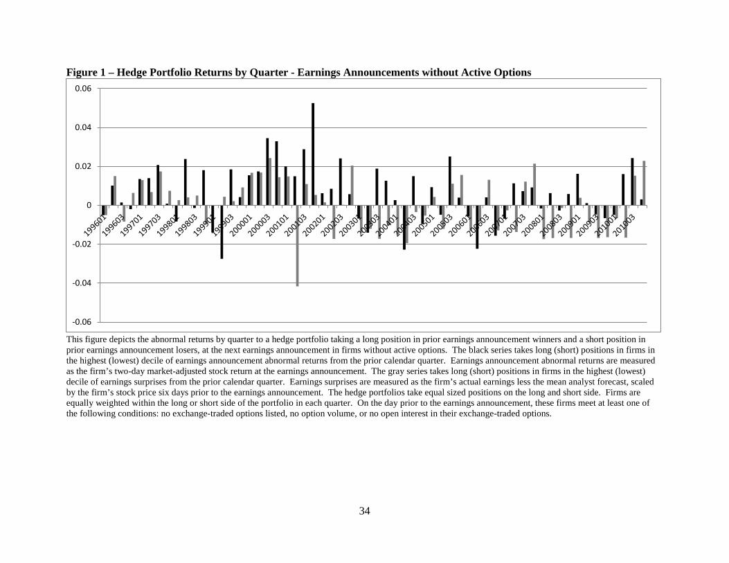
34

Figure 1 – Hedge Portfolio Returns by Quarter - Earnings Announcements without Active Options

This figure depicts the abnormal returns by quarter to a hedge portfolio taking a long position in prior earnings announcement winners and a short position in prior earnings announcement losers, at the next earnings announcement in firms without active options. The black series takes long (short) positions in firms in the highest (lowest) decile of earnings announcement abnormal returns from the prior calendar quarter. Earnings announcement abnormal returns are measured as the firm’s two-day market-adjusted stock return at the earnings announcement. The gray series takes long (short) positions in firms in the highest (lowest) decile of earnings surprises from the prior calendar quarter. Earnings surprises are measured as the firm’s actual earnings less the mean analyst forecast, scaled by the firm’s stock price six days prior to the earnings announcement. The hedge portfolios take equal sized positions on the long and short side. Firms are equally weighted within the long or short side of the portfolio in each quarter. On the day prior to the earnings announcement, these firms meet at least one of the following conditions: no exchange-traded options listed, no option volume, or no open interest in their exchange-traded options.

-0.06

-0.04

-0.02

0

0.02

0.04

0.06

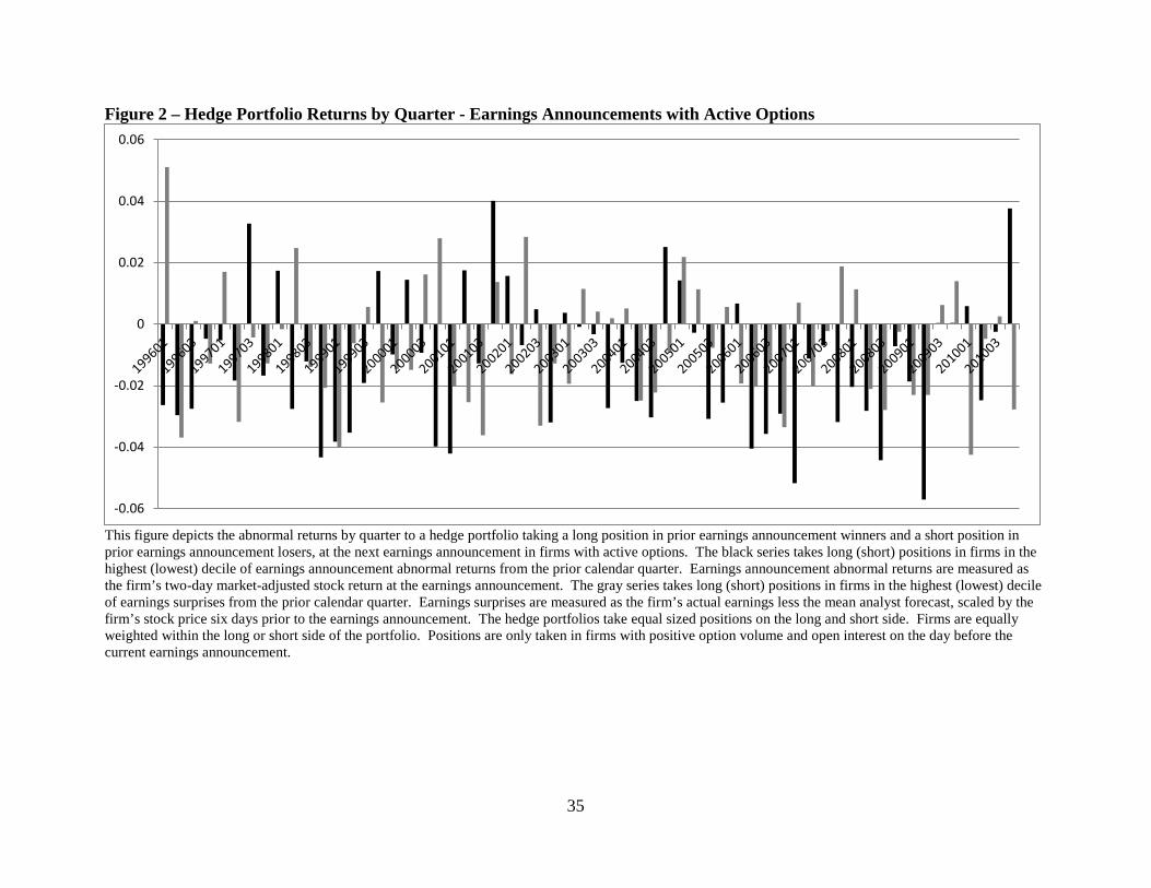
35

Figure 2 – Hedge Portfolio Returns by Quarter - Earnings Announcements with Active Options

This figure depicts the abnormal returns by quarter to a hedge portfolio taking a long position in prior earnings announcement winners and a short position in prior earnings announcement losers, at the next earnings announcement in firms with active options. The black series takes long (short) positions in firms in the highest (lowest) decile of earnings announcement abnormal returns from the prior calendar quarter. Earnings announcement abnormal returns are measured as the firm’s two-day market-adjusted stock return at the earnings announcement. The gray series takes long (short) positions in firms in the highest (lowest) decile of earnings surprises from the prior calendar quarter. Earnings surprises are measured as the firm’s actual earnings less the mean analyst forecast, scaled by the firm’s stock price six days prior to the earnings announcement. The hedge portfolios take equal sized positions on the long and short side. Firms are equally weighted within the long or short side of the portfolio. Positions are only taken in firms with positive option volume and open interest on the day before the current earnings announcement.

-0.06

-0.04

-0.02

0

0.02

0.04

0.06

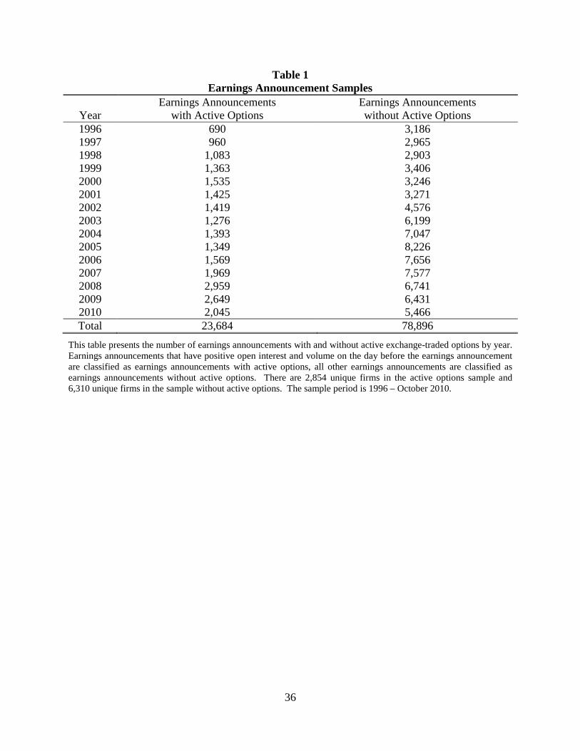
36

Table 1 Earnings Announcement Samples

Year

Earnings Announcements with Active Options

Earnings Announcements without Active Options

1996 690 3,186 1997 960 2,965 1998 1,083 2,903 1999 1,363 3,406 2000 1,535 3,246 2001 1,425 3,271 2002 1,419 4,576 2003 1,276 6,199 2004 1,393 7,047 2005 1,349 8,226 2006 1,569 7,656 2007 1,969 7,577 2008 2,959 6,741 2009 2,649 6,431 2010 2,045 5,466 Total 23,684 78,896

This table presents the number of earnings announcements with and without active exchange-traded options by year. Earnings announcements that have positive open interest and volume on the day before the earnings announcement are classified as earnings announcements with active options, all other earnings announcements are classified as earnings announcements without active options. There are 2,854 unique firms in the active options sample and 6,310 unique firms in the sample without active options. The sample period is 1996 – October 2010.

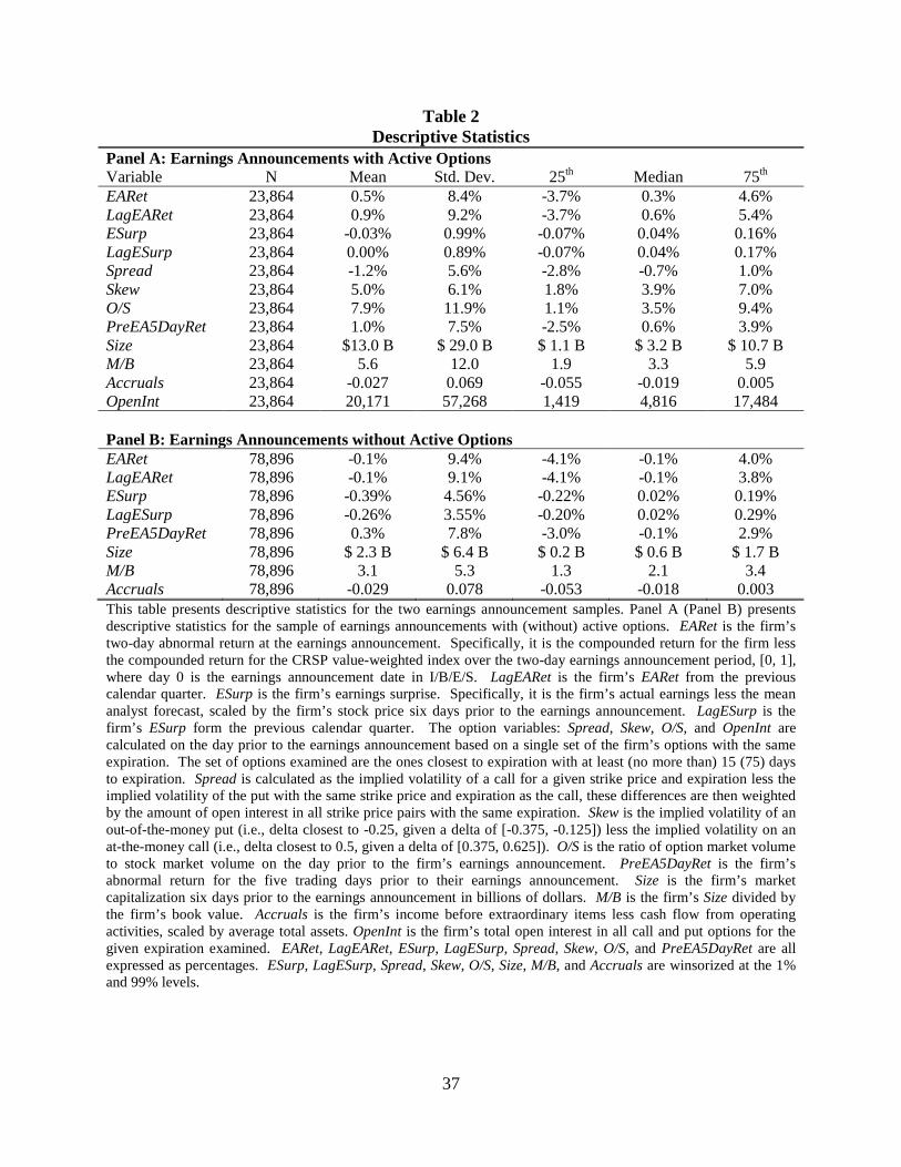
37

Table 2 Descriptive Statistics

Panel A: Earnings Announcements with Active Options Variable N Mean Std. Dev. 25th Median 75th EARet 23,864 0.5% 8.4% -3.7% 0.3% 4.6% LagEARet 23,864 0.9% 9.2% -3.7% 0.6% 5.4% ESurp 23,864 -0.03% 0.99% -0.07% 0.04% 0.16% LagESurp 23,864 0.00% 0.89% -0.07% 0.04% 0.17% Spread 23,864 -1.2% 5.6% -2.8% -0.7% 1.0% Skew 23,864 5.0% 6.1% 1.8% 3.9% 7.0% O/S 23,864 7.9% 11.9% 1.1% 3.5% 9.4% PreEA5DayRet 23,864 1.0% 7.5% -2.5% 0.6% 3.9% Size 23,864 $13.0 B $ 29.0 B $ 1.1 B $ 3.2 B $ 10.7 B M/B 23,864 5.6 12.0 1.9 3.3 5.9 Accruals 23,864 -0.027 0.069 -0.055 -0.019 0.005 OpenInt 23,864 20,171 57,268 1,419 4,816 17,484 Panel B: Earnings Announcements without Active Options EARet 78,896 -0.1% 9.4% -4.1% -0.1% 4.0% LagEARet 78,896 -0.1% 9.1% -4.1% -0.1% 3.8% ESurp 78,896 -0.39% 4.56% -0.22% 0.02% 0.19% LagESurp 78,896 -0.26% 3.55% -0.20% 0.02% 0.29% PreEA5DayRet 78,896 0.3% 7.8% -3.0% -0.1% 2.9% Size 78,896 $ 2.3 B $ 6.4 B $ 0.2 B $ 0.6 B $ 1.7 B M/B 78,896 3.1 5.3 1.3 2.1 3.4 Accruals 78,896 -0.029 0.078 -0.053 -0.018 0.003 This table presents descriptive statistics for the two earnings announcement samples. Panel A (Panel B) presents descriptive statistics for the sample of earnings announcements with (without) active options. EARet is the firm’s two-day abnormal return at the earnings announcement. Specifically, it is the compounded return for the firm less the compounded return for the CRSP value-weighted index over the two-day earnings announcement period, [0, 1], where day 0 is the earnings announcement date in I/B/E/S. LagEARet is the firm’s EARet from the previous calendar quarter. ESurp is the firm’s earnings surprise. Specifically, it is the firm’s actual earnings less the mean analyst forecast, scaled by the firm’s stock price six days prior to the earnings announcement. LagESurp is the firm’s ESurp form the previous calendar quarter. The option variables: Spread, Skew, O/S, and OpenInt are calculated on the day prior to the earnings announcement based on a single set of the firm’s options with the same expiration. The set of options examined are the ones closest to expiration with at least (no more than) 15 (75) days to expiration. Spread is calculated as the implied volatility of a call for a given strike price and expiration less the implied volatility of the put with the same strike price and expiration as the call, these differences are then weighted by the amount of open interest in all strike price pairs with the same expiration. Skew is the implied volatility of an out-of-the-money put (i.e., delta closest to -0.25, given a delta of [-0.375, -0.125]) less the implied volatility on an at-the-money call (i.e., delta closest to 0.5, given a delta of [0.375, 0.625]). O/S is the ratio of option market volume to stock market volume on the day prior to the firm’s earnings announcement. PreEA5DayRet is the firm’s abnormal return for the five trading days prior to their earnings announcement. Size is the firm’s market capitalization six days prior to the earnings announcement in billions of dollars. M/B is the firm’s Size divided by the firm’s book value. Accruals is the firm’s income before extraordinary items less cash flow from operating activities, scaled by average total assets. OpenInt is the firm’s total open interest in all call and put options for the given expiration examined. EARet, LagEARet, ESurp, LagESurp, Spread, Skew, O/S, and PreEA5DayRet are all expressed as percentages. ESurp, LagESurp, Spread, Skew, O/S, Size, M/B, and Accruals are winsorized at the 1% and 99% levels.

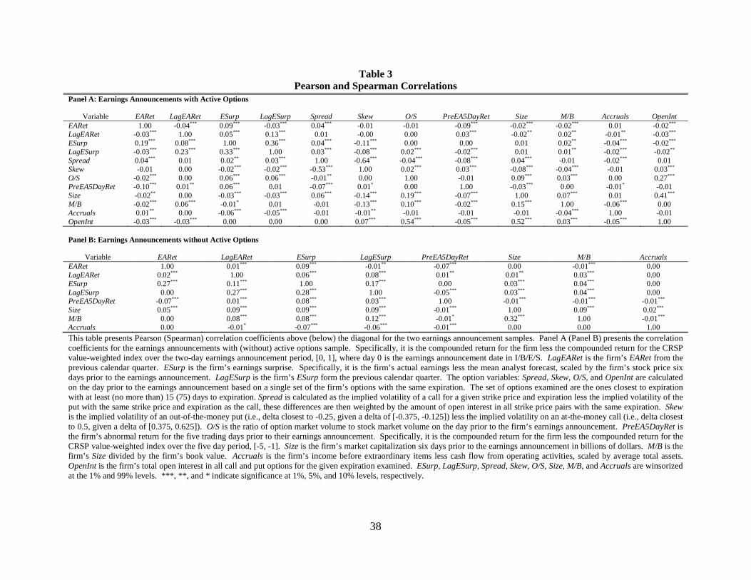
38

Table 3 Pearson and Spearman Correlations

Panel B: Earnings Announcements without Active Options

Variable EARet LagEARet ESurp LagESurp PreEA5DayRet Size M/B Accruals EARet 1.00 0.01*** 0.09*** -0.01** -0.07*** 0.00 -0.01*** 0.00 LagEARet 0.02*** 1.00 0.06*** 0.08*** 0.01** 0.01** 0.03*** 0.00 ESurp 0.27*** 0.11*** 1.00 0.17*** 0.00 0.03*** 0.04*** 0.00 LagESurp 0.00 0.27*** 0.28*** 1.00 -0.05*** 0.03*** 0.04*** 0.00 PreEA5DayRet -0.07*** 0.01*** 0.08*** 0.03*** 1.00 -0.01*** -0.01*** -0.01*** Size 0.05*** 0.09*** 0.09*** 0.09*** -0.01*** 1.00 0.09*** 0.02*** M/B 0.00 0.08*** 0.08*** 0.12*** -0.01* 0.32*** 1.00 -0.01*** Accruals 0.00 -0.01* -0.07*** -0.06*** -0.01*** 0.00 0.00 1.00 This table presents Pearson (Spearman) correlation coefficients above (below) the diagonal for the two earnings announcement samples. Panel A (Panel B) presents the correlation coefficients for the earnings announcements with (without) active options sample. Specifically, it is the compounded return for the firm less the compounded return for the CRSP value-weighted index over the two-day earnings announcement period, [0, 1], where day 0 is the earnings announcement date in I/B/E/S. LagEARet is the firm’s EARet from the previous calendar quarter. ESurp is the firm’s earnings surprise. Specifically, it is the firm’s actual earnings less the mean analyst forecast, scaled by the firm’s stock price six days prior to the earnings announcement. LagESurp is the firm’s ESurp form the previous calendar quarter. The option variables: Spread, Skew, O/S, and OpenInt are calculated on the day prior to the earnings announcement based on a single set of the firm’s options with the same expiration. The set of options examined are the ones closest to expiration with at least (no more than) 15 (75) days to expiration. Spread is calculated as the implied volatility of a call for a given strike price and expiration less the implied volatility of the put with the same strike price and expiration as the call, these differences are then weighted by the amount of open interest in all strike price pairs with the same expiration. Skew is the implied volatility of an out-of-the-money put (i.e., delta closest to -0.25, given a delta of [-0.375, -0.125]) less the implied volatility on an at-the-money call (i.e., delta closest to 0.5, given a delta of [0.375, 0.625]). O/S is the ratio of option market volume to stock market volume on the day prior to the firm’s earnings announcement. PreEA5DayRet is the firm’s abnormal return for the five trading days prior to their earnings announcement. Specifically, it is the compounded return for the firm less the compounded return for the CRSP value-weighted index over the five day period, [-5, -1]. Size is the firm’s market capitalization six days prior to the earnings announcement in billions of dollars. M/B is the firm’s Size divided by the firm’s book value. Accruals is the firm’s income before extraordinary items less cash flow from operating activities, scaled by average total assets. OpenInt is the firm’s total open interest in all call and put options for the given expiration examined. ESurp, LagESurp, Spread, Skew, O/S, Size, M/B, and Accruals are winsorized at the 1% and 99% levels. ***, **, and * indicate significance at 1%, 5%, and 10% levels, respectively.

Panel A: Earnings Announcements with Active Options

Variable EARet LagEARet ESurp LagESurp Spread Skew O/S PreEA5DayRet Size M/B Accruals OpenInt EARet 1.00 -0.04*** 0.09*** -0.03*** 0.04*** -0.01 -0.01 -0.09*** -0.02*** -0.02*** 0.01 -0.02*** LagEARet -0.03*** 1.00 0.05*** 0.13*** 0.01 -0.00 0.00 0.03*** -0.02** 0.02** -0.01** -0.03*** ESurp 0.19*** 0.08*** 1.00 0.36*** 0.04*** -0.11*** 0.00 0.00 0.01 0.02** -0.04*** -0.02*** LagESurp -0.03*** 0.23*** 0.33*** 1.00 0.03*** -0.08*** 0.02*** -0.02*** 0.01 0.01** -0.02*** -0.02** Spread 0.04*** 0.01 0.02** 0.03*** 1.00 -0.64*** -0.04*** -0.08*** 0.04*** -0.01 -0.02*** 0.01 Skew -0.01 0.00 -0.02*** -0.02*** -0.53*** 1.00 0.02*** 0.03*** -0.08*** -0.04*** -0.01 0.03*** O/S -0.02*** 0.00 0.06*** 0.06*** -0.01** 0.00 1.00 -0.01 0.09*** 0.03*** 0.00 0.27*** PreEA5DayRet -0.10*** 0.01** 0.06*** 0.01 -0.07*** 0.01* 0.00 1.00 -0.03*** 0.00 -0.01* -0.01 Size -0.02** 0.00 -0.03*** -0.03*** 0.06*** -0.14*** 0.19*** -0.07*** 1.00 0.07*** 0.01 0.41*** M/B -0.02*** 0.06*** -0.01* 0.01 -0.01 -0.13*** 0.10*** -0.02*** 0.15*** 1.00 -0.06*** 0.00 Accruals 0.01** 0.00 -0.06*** -0.05*** -0.01 -0.01** -0.01 -0.01 -0.01 -0.04*** 1.00 -0.01 OpenInt -0.03*** -0.03*** 0.00 0.00 0.00 0.07*** 0.54*** -0.05*** 0.52*** 0.03*** -0.05*** 1.00

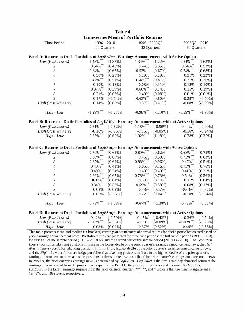
39

Table 4 Time-series Mean of Portfolio Returns

Time Period 1996 – 2010 60 Quarters

1996 - 2003Q2 30 Quarters

2003Q3 – 2010 30 Quarters

Panel A: Returns to Decile Portfolios of LagEARet - Earnings Announcements with Active Options

Low (Past Losers) 2 3 4 5 6 7

1.43%*** 0.54%**

0.64%*** 0.30%

0.42%*** 0.10%

0.37%**

[1.37%] [0.46%] [0.67%] [0.23%] [0.51%] [0.18%] [0.39%]

1.34%*** 0.44%

0.53%** 0.29%

0.64%*** 0.08%

0.60%**

[1.22%] [0.35%] [0.67%] [0.29%] [0.81%] [0.31%] [0.74%]

1.51%*** 0.64%**

0.74%*** 0.31% 0.21% 0.12% 0.15%

[1.63%] [0.53%] [0.68%] [0.22%] [0.26%] [0.10%] [0.19%]

8 0.21% [0.07%] 0.40% [0.08%] 0.01% [0.01%] 9 0.17% [-0.14%] 0.63%** [0.80%] -0.28% [-0.50%]

High (Past Winners) 0.14% [0.08%] 0.37% [0.41%] -0.08% [-0.09%]

High - Low -1.29%*** [-1.27%] -0.98%** [-1.10%] -1.59%*** [-1.95%]

Panel B: Returns to Decile Portfolios of LagEARet - Earnings Announcements without Active Options Low (Past Losers)

High (Past Winners) High - Low

-0.81%*** -0.16%

0.65%***

[-0.82%] [-0.16%] [0.60%]

-1.18%*** -0.16%

1.02%***

[-0.99%] [-0.05%] [1.18%]

-0.44%** -0.16% 0.28%

[-0.40%] [-0.24%] [0.35%]

Panel C: Returns to Decile Portfolios of LagESurp - Earnings Announcements with Active Options

Low (Past Losers) 2

0.79%*** 0.60%***

[0.65%] [0.69%]

0.89%*** 0.46%

[0.62%] [0.58%]

0.68%*** 0.73%***

[0.75%] [0.83%]

3 0.67%*** [0.62%] 0.88%*** [0.96%] 0.47%** [0.51%] 4 0.40%** [0.41%] 0.05% [0.16%] 0.75%*** [0.76%] 5 0.40%** [0.34%] 0.40% [0.49%] 0.41%** [0.31%] 6 0.66%*** [0.67%] 0.78%*** [0.73%] 0.54%** [0.56%] 7 0.37%* [0.04%] 0.53% [0.14%] 0.21% [0.04%] 8 0.34%** [0.37%] 0.59%** [0.58%] 0.08% [0.17%] 9 0.02% [0.02%] 0.48% [0.57%] -0.43%* [-0.32%]

High (Past Winners) 0.06% [-0.07%] 0.22% [0.04%] -0.10% [-0.34%]

High - Low -0.73%*** [-1.08%] -0.67%** [-1.28%] -0.78%** [-0.62%]

Panel D: Returns to Decile Portfolios of LagESurp - Earnings Announcements without Active Options Low (Past Losers)

High (Past Winners) High - Low

-0.42%** -0.45%***

-0.03%

[-0.50%] [-0.39%] [0.09%]

-0.47%* -0.10% 0.37%

[-0.42%] [-0.09%] [0.52%]

-0.36% -0.80%***

-0.44%*

[-0.54%] [-0.75%] [-0.85%]

This table presents mean and median (in brackets) earnings announcement abnormal returns for decile portfolios created based on prior earnings announcement news. Portfolio returns are presented for three time periods: the full sample period (1996 - 2010), the first half of the sample period (1996 – 2003Q2), and the second half of the sample period (2003Q3 - 2010). The Low (Past Losers) portfolios take long positions in firms in the lowest decile of the prior quarter’s earnings announcement news, the High (Past Winners) portfolios take long positions in firms in the highest decile of the prior quarter’s earnings announcement news, and the High - Low portfolios are hedge portfolios that take long positions in firms in the highest decile of the prior quarter’s earnings announcement news and short positions in firms in the lowest decile of the prior quarter’s earnings announcement news. In Panel A, the prior quarter’s earnings news is determined by LagEARet. LagEARet is the firm’s two-day abnormal return at the earnings announcement from the prior calendar quarter. In Panel B, the prior earnings news is determined by LagESurp. LagESurp is the firm’s earnings surprise from the prior calendar quarter. ***, **, and * indicate that the mean is significant at 1%, 5%, and 10% levels, respectively.

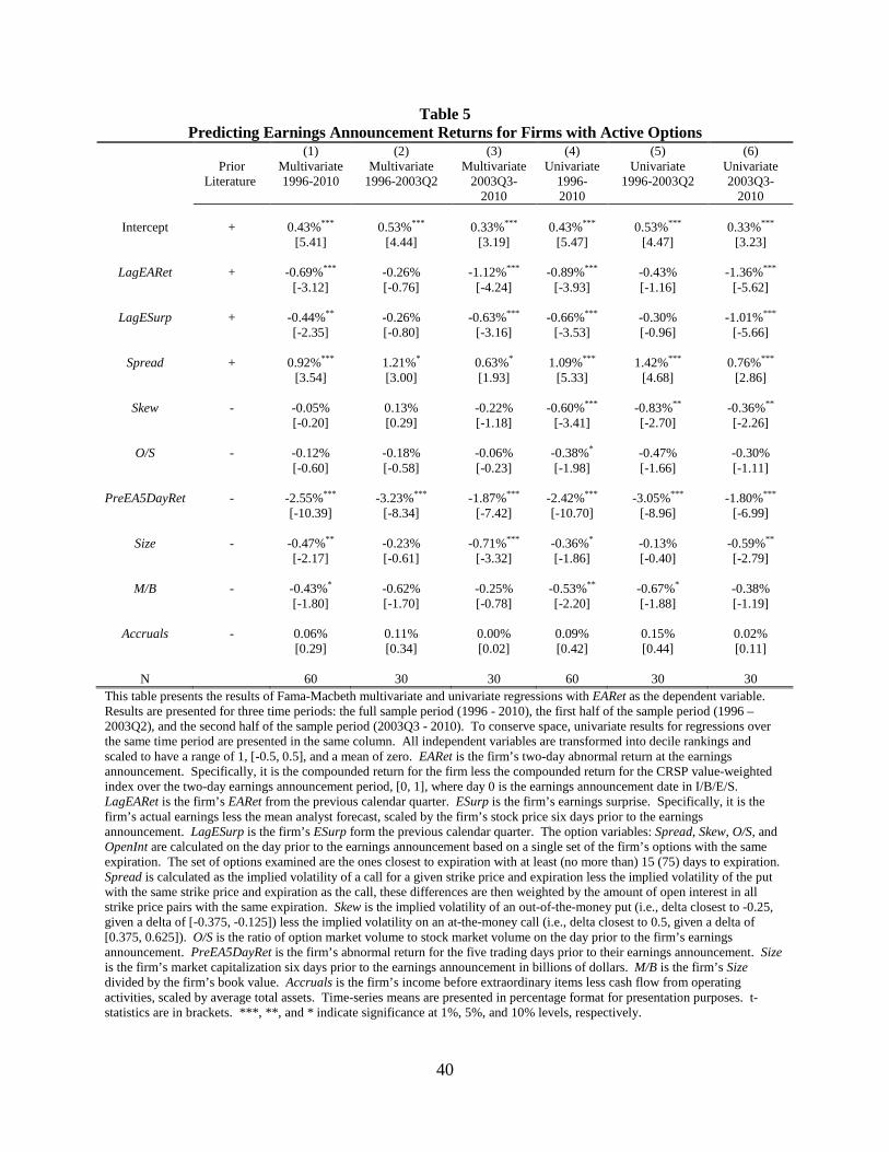
40

Table 5 Predicting Earnings Announcement Returns for Firms with Active Options

(1) (2) (3) (4) (5) (6) Prior Multivariate Multivariate Multivariate Univariate Univariate Univariate Literature

1996-2010 1996-2003Q2 2003Q3-

2010 1996-2010

1996-2003Q2 2003Q3-2010

Intercept + 0.43%*** 0.53%*** 0.33%*** 0.43%*** 0.53%*** 0.33%***

[5.41] [4.44] [3.19] [5.47] [4.47] [3.23]

LagEARet + -0.69%*** -0.26% -1.12%*** -0.89%*** -0.43% -1.36%*** [-3.12] [-0.76] [-4.24] [-3.93] [-1.16] [-5.62]

LagESurp + -0.44%** -0.26% -0.63%*** -0.66%*** -0.30% -1.01%*** [-2.35] [-0.80] [-3.16] [-3.53] [-0.96] [-5.66]

Spread + 0.92%*** 1.21%* 0.63%* 1.09%*** 1.42%*** 0.76%*** [3.54] [3.00] [1.93] [5.33] [4.68] [2.86]

Skew - -0.05% 0.13% -0.22% -0.60%*** -0.83%** -0.36%** [-0.20] [0.29] [-1.18] [-3.41] [-2.70] [-2.26]

O/S - -0.12% -0.18% -0.06% -0.38%* -0.47% -0.30% [-0.60] [-0.58] [-0.23] [-1.98] [-1.66] [-1.11]

PreEA5DayRet - -2.55%*** -3.23%*** -1.87%*** -2.42%*** -3.05%*** -1.80%*** [-10.39] [-8.34] [-7.42] [-10.70] [-8.96] [-6.99]

Size - -0.47%** -0.23% -0.71%*** -0.36%* -0.13% -0.59%** [-2.17] [-0.61] [-3.32] [-1.86] [-0.40] [-2.79]

M/B - -0.43%* -0.62% -0.25% -0.53%** -0.67%* -0.38% [-1.80] [-1.70] [-0.78] [-2.20] [-1.88] [-1.19]

Accruals - 0.06% 0.11% 0.00% 0.09% 0.15% 0.02% [0.29] [0.34] [0.02] [0.42] [0.44] [0.11]

N 60 30 30 60 30 30 This table presents the results of Fama-Macbeth multivariate and univariate regressions with EARet as the dependent variable. Results are presented for three time periods: the full sample period (1996 - 2010), the first half of the sample period (1996 – 2003Q2), and the second half of the sample period (2003Q3 - 2010). To conserve space, univariate results for regressions over the same time period are presented in the same column. All independent variables are transformed into decile rankings and scaled to have a range of 1, [-0.5, 0.5], and a mean of zero. EARet is the firm’s two-day abnormal return at the earnings announcement. Specifically, it is the compounded return for the firm less the compounded return for the CRSP value-weighted index over the two-day earnings announcement period, [0, 1], where day 0 is the earnings announcement date in I/B/E/S. LagEARet is the firm’s EARet from the previous calendar quarter. ESurp is the firm’s earnings surprise. Specifically, it is the firm’s actual earnings less the mean analyst forecast, scaled by the firm’s stock price six days prior to the earnings announcement. LagESurp is the firm’s ESurp form the previous calendar quarter. The option variables: Spread, Skew, O/S, and OpenInt are calculated on the day prior to the earnings announcement based on a single set of the firm’s options with the same expiration. The set of options examined are the ones closest to expiration with at least (no more than) 15 (75) days to expiration. Spread is calculated as the implied volatility of a call for a given strike price and expiration less the implied volatility of the put with the same strike price and expiration as the call, these differences are then weighted by the amount of open interest in all strike price pairs with the same expiration. Skew is the implied volatility of an out-of-the-money put (i.e., delta closest to -0.25, given a delta of [-0.375, -0.125]) less the implied volatility on an at-the-money call (i.e., delta closest to 0.5, given a delta of [0.375, 0.625]). O/S is the ratio of option market volume to stock market volume on the day prior to the firm’s earnings announcement. PreEA5DayRet is the firm’s abnormal return for the five trading days prior to their earnings announcement. Size is the firm’s market capitalization six days prior to the earnings announcement in billions of dollars. M/B is the firm’s Size divided by the firm’s book value. Accruals is the firm’s income before extraordinary items less cash flow from operating activities, scaled by average total assets. Time-series means are presented in percentage format for presentation purposes. t-statistics are in brackets. ***, **, and * indicate significance at 1%, 5%, and 10% levels, respectively.

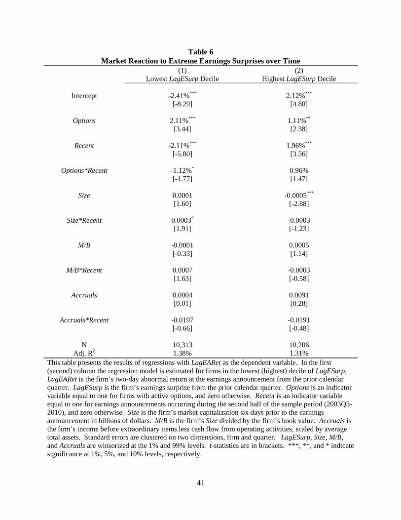
41

Table 6 Market Reaction to Extreme Earnings Surprises over Time

(1) (2) Lowest LagESurp Decile Highest LagESurp Decile

Intercept -2.41%*** 2.12%*** [-8.29] [4.80]

Options 2.11%*** 1.11%** [3.44] [2.38]

Recent -2.11%*** 1.96%*** [-5.80] [3.56]

Options*Recent -1.12%* 0.96% [-1.77] [1.47]

Size 0.0001 -0.0005*** [1.60] [-2.88]

Size*Recent 0.0003* -0.0003 [1.91] [-1.23]

M/B -0.0001 0.0005 [-0.33] [1.14]

M/B*Recent 0.0007 -0.0003 [1.63] [-0.58]

Accruals 0.0004 0.0091 [0.01] [0.28]

Accruals*Recent -0.0197 -0.0191 [-0.66] [-0.48]

N Adj. R2

10,313 1.38%

10,206 1.31%

This table presents the results of regressions with LagEARet as the dependent variable. In the first (second) column the regression model is estimated for firms in the lowest (highest) decile of LagESurp. LagEARet is the firm’s two-day abnormal return at the earnings announcement from the prior calendar quarter. LagESurp is the firm’s earnings surprise from the prior calendar quarter. Options is an indicator variable equal to one for firms with active options, and zero otherwise. Recent is an indicator variable equal to one for earnings announcements occurring during the second half of the sample period (2003Q3-2010), and zero otherwise. Size is the firm’s market capitalization six days prior to the earnings announcement in billions of dollars. M/B is the firm’s Size divided by the firm’s book value. Accruals is the firm’s income before extraordinary items less cash flow from operating activities, scaled by average total assets. Standard errors are clustered on two dimensions, firm and quarter. LagESurp, Size, M/B, and Accruals are winsorized at the 1% and 99% levels. t-statistics are in brackets. ***, **, and * indicate significance at 1%, 5%, and 10% levels, respectively.

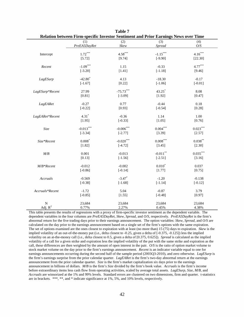
42

Table 7 Relation between Firm-specific Investor Sentiment and Prior Earnings News over Time

(1) (2) (3) (4) PreEA5DayRet Skew Spread O/S

Intercept 1.72*** 4.58*** -1.15*** 4.16*** [5.72] [9.74] [-9.90] [22.30]

Recent -1.09*** 1.15 -0.33 4.77*** [-3.20] [1.41] [-1.18] [9.46]

LagESurp -42.80* 4.13 -18.30 -0.17 [-1.67] [0.22] [-1.06] [-0.01]

LagESurp*Recent 27.99 -75.73*** 43.25* 8.08 [0.81] [-3.09] [1.92] [0.47]

LagEARet -0.27 0.77 -0.44 0.18 [-0.22] [0.93] [-0.54] [0.28]

LagEARet*Recent 4.31* -0.36 1.14 1.00 [1.95] [-0.33] [1.05] [0.76]

Size -0.013*** -0.006*** 0.004*** 0.023*** [-3.34] [-2.77] [3.39] [2.57]

Size*Recent 0.008* -0.020*** 0.008*** 0.038** [1.82] [-4.72] [3.45] [2.30]

M/B 0.001 -0.013 -0.011** 0.035*** [0.13] [-1.56] [-2.51] [3.16]

M/B*Recent -0.012 -0.002 0.010* 0.037 [-0.86] [-0.14] [1.77] [0.75]

Accruals -0.569 -3.47* -1.20 -0.138 [-0.38] [-1.68] [-1.14] [-0.12]

Accruals*Recent -1.72 5.04 -0.87 3.79 [-0.85] [1.55] [-0.48] [0.97]

N 23,684 23,684 23,684 23,684 Adj. R2 0.77% 2.27% 0.45% 4.38%

This table presents the results of regressions with a proxy of firm-specific investor sentiment as the dependent variable. The dependent variables in the four columns are PreEA5DayRet, Skew, Spread, and O/S, respectively. PreEA5DayRet is the firm’s abnormal return for the five trading days prior to their earnings announcement. The option variables: Skew, Spread, and O/S are calculated on the day prior to the earnings announcement based on a single set of the firm’s options with the same expiration. The set of options examined are the ones closest to expiration with at least (no more than) 15 (75) days to expiration. Skew is the implied volatility of an out-of-the-money put (i.e., delta closest to -0.25, given a delta of [-0.375, -0.125]) less the implied volatility on an at-the-money call (i.e., delta closest to 0.5, given a delta of [0.375, 0.625]). Spread is calculated as the implied volatility of a call for a given strike and expiration less the implied volatility of the put with the same strike and expiration as the call, these differences are then weighted by the amount of open interest in the pair. O/S is the ratio of option market volume to stock market volume on the day prior to the firm’s earnings announcement. Recent is an indicator variable equal to one for earnings announcements occurring during the second half of the sample period (2003Q3-2010), and zero otherwise. LagESurp is the firm’s earnings surprise from the prior calendar quarter. LagEARet is the firm’s two-day abnormal return at the earnings announcement from the prior calendar quarter. Size is the firm’s market capitalization six days prior to the earnings announcement in billions of dollars. M/B is the firm’s Size divided by the firm’s book value. Accruals is the firm’s income before extraordinary items less cash flow from operating activities, scaled by average total assets. LagESurp, Size, M/B, and Accruals are winsorized at the 1% and 99% levels. Standard errors are clustered on two dimensions, firm and quarter. t-statistics are in brackets. ***, **, and * indicate significance at 1%, 5%, and 10% levels, respectively.

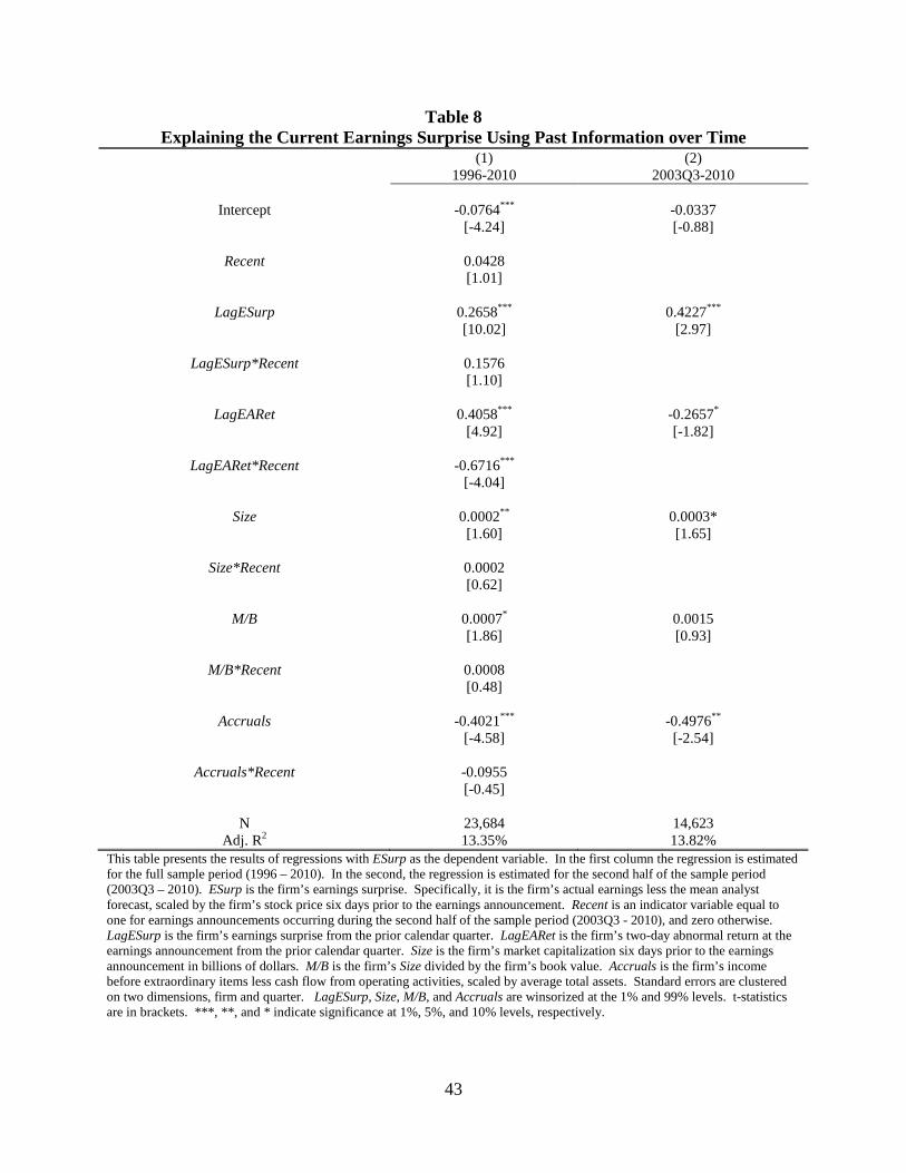
43

Table 8 Explaining the Current Earnings Surprise Using Past Information over Time

(1) (2) 1996-2010 2003Q3-2010

Intercept -0.0764*** -0.0337 [-4.24] [-0.88]

Recent 0.0428 [1.01]

LagESurp 0.2658*** 0.4227*** [10.02] [2.97]

LagESurp*Recent 0.1576 [1.10]

LagEARet 0.4058*** -0.2657* [4.92] [-1.82]

LagEARet*Recent -0.6716*** [-4.04]

Size 0.0002** 0.0003* [1.60] [1.65]

Size*Recent 0.0002 [0.62]

M/B 0.0007* 0.0015 [1.86] [0.93]

M/B*Recent 0.0008 [0.48]

Accruals -0.4021*** -0.4976** [-4.58] [-2.54]

Accruals*Recent -0.0955 [-0.45]

N 23,684 14,623 Adj. R2 13.35% 13.82%

This table presents the results of regressions with ESurp as the dependent variable. In the first column the regression is estimated for the full sample period (1996 – 2010). In the second, the regression is estimated for the second half of the sample period (2003Q3 – 2010). ESurp is the firm’s earnings surprise. Specifically, it is the firm’s actual earnings less the mean analyst forecast, scaled by the firm’s stock price six days prior to the earnings announcement. Recent is an indicator variable equal to one for earnings announcements occurring during the second half of the sample period (2003Q3 - 2010), and zero otherwise. LagESurp is the firm’s earnings surprise from the prior calendar quarter. LagEARet is the firm’s two-day abnormal return at the earnings announcement from the prior calendar quarter. Size is the firm’s market capitalization six days prior to the earnings announcement in billions of dollars. M/B is the firm’s Size divided by the firm’s book value. Accruals is the firm’s income before extraordinary items less cash flow from operating activities, scaled by average total assets. Standard errors are clustered on two dimensions, firm and quarter. LagESurp, Size, M/B, and Accruals are winsorized at the 1% and 99% levels. t-statistics are in brackets. ***, **, and * indicate significance at 1%, 5%, and 10% levels, respectively.