Overtone Mobility Spectrometry: Part 3. On the Origin of Peaks

B American Society for Mass Spectrometry, 2011DOI: 10.1007/s13361-011-0087-yJ. Am. Soc. Mass Spectrom. (2011) 22:804Y816

RESEARCH ARTICLE

Overtone Mobility Spectrometry: Part 3.On the Origin of Peaks

Stephen J. Valentine,1 Ruwan T. Kurulugama,2 David E. Clemmer1

1Department of Chemistry, Indiana University, Bloomington, IN, 47405, USA2Pacific Northwest National Laboratory, Richland, WA, USA

AbstractThe origin of non-integer overtone peaks in overtone mobility spectrometry (OMS) spectra isinvestigated by ion trajectory simulations. Simulations indicate that these OMS features arisefrom higher-order overtone series. An empirically-derived formula is presented as a means ofdescribing the positions of peaks. The new equation makes it possible to determine collisioncross sections from any OMS peak. Additionally, it is extended as a means of predicting theresolving power for any peak in an OMS distribution.

Key words: Ion mobility spectrometry, Overtone mobility spectrometry, Mass spectrometry

Introduction

The recent application of ion mobility spectrometry(IMS) for the characterization of complex mixtures [1–

14] and the development of hybrid IMS techniques [15–25]has generated interest in improving the resolution ofmobility separations. The resolving power (RIMS) of mobilityseparations depends on the drift field (E), the drift length (L),and the temperature (T) of the buffer gas according to [26]

tD�tD

¼ LEze

16kBT ln 2

� �1=2

ð1Þ

In Equation 1, tD, ΔtD, kb, and ze correspond to the drifttime of the ion, the full width at half-maximum (FWHM) ofthe drift time peak, Boltzmann’s constant, and the charge ofthe ion, respectively. Instrumental developments have led toa number of high-resolution drift tube designs exhibitingresolving powers that range from ~100 to 250 [24, 27–34].The square root dependence on the parameters: E, L, and T

make it difficult to develop higher resolving power instru-ments with incremental changes in instrument design. Forexample, doubling the length of the drift region onlyincreases RIMS by a factor of 1.41.

Recently, the technique of overtone mobility spectrome-try (OMS) has been introduced as a means of separating ions[35, 36]. In this approach, drift fields are applied in a time-dependent manner, resulting in the transmission of ions withmobilities that are resonant to the field application fre-quency. Theoretical considerations led to an equationrelating the OMS resolving power (ROMS) to experimentalparameters associated with instrumentation geometry and theIMS resolving power (RIMS) as shown in Equation 2 [36].

ROMS ¼ 1

1� 1� C2RIMS

h imn� f�1� le

ltþle½ �mn

� � ð2Þ

The variables Φ, m, and n correspond to the OMSoperational parameters the phase number of the system(number of distinct field applications settings), the fieldapplication harmonic number, and the number of OMS drifttube segments, respectively. The variables le and lt are thelengths of ion elimination and ion transmission regions (seebelow), respectively. C2 is a constant allowing the compar-ison to RIMS. ROMS is expressed for experimental data as f/Δf

(1)

Received: 15 October 2010Revised: 15 January 2011Accepted: 18 January 2011Published online: 4 March 2011

Electronic supplementary material The online version of this article(doi:10.1007/s13361-011-0087-y) contains supplementary material, whichis available to authorized users.

Correspondence to: David E. Clemmer; e-mail: [email protected]

http://dx.doi.org/10.1007/s13361-011-0087-y

where f is the frequency of the peak in the OMS distributionand Δf is obtained at FWHM.

Equation 2 shows that ROMS is proportional to m and nindicating that higher resolution separations can be obtained(compared with RIMS) for incremental changes in instrumen-tation parameters. Recently, high-resolution OMS separa-tions (ROMS 9 200) of gas-phase ubiquitin ions have beenreported [37]. Separate experiments employing a circulardrift tube operated in an OMS mode yielded peaks withROMS 9 400 [38]. Such high resolving powers are obtainablebecause the ions travel around the circular drift tube morethan 60 times thereby increasing n. Improvements in ROMS

come at a cost to overall sensitivity. Ion loss results from theincreased selectivity of the mobility filtering process,decreased ion transmission through gridded lenses, andincreased ion diffusion for measurements with extendedexperimental timescales. Thus, high-resolution OMS sepa-rations are currently less sensitive than lower-resolutioncommercial instrumentation employing mobility separations.That said, these examples demonstrate how Equation 2provides insight that is useful for experimental analyses.Recently, a frequency scanning method for OMS experi-ments employing a circular drift tube has been demonstratedfor high-efficiency separation of components in a trypticdigest mixture [38].

Although Equation 2 estimates ROMS of many peaks, itfails to estimate ROMS values for a series of peaks centered atfrequencies that are non-integer multiples of the fundamentaltransmission frequency (ff). The largest of these featuresoccurs between the ff peak and the next major harmonicpeak. These peaks are often sharp, having ROMS values thatare higher than the neighboring major harmonic peaks. Inthe work presented here, we use ion trajectory simulations toprovide insight into the origin of these peaks as well as thefactors that contribute to increased ROMS. We use this insightto develop a mathematical framework for describing thepositions and shapes of all peaks (ff and overtones). Theresulting information suggests that it should be possible totailor OMS separations to the frequency region in whichthese higher-resolution overtone peaks are found in order toachieve higher separation efficiency.

ExperimentalOMS Measurements

General aspects of IMS theory [26, 39–42], instrumenta-tion [17, 18, 22, 24, 43, 44], and techniques [45–47] havebeen discussed in detail elsewhere. Additionally, OMSseparations have been described in detail, including themethod of mobility selection, operational modes of OMSdevices, and theoretical considerations of ROMS [36].Briefly, an OMS instrument contains a segmented drifttube. Adjoining drift segment (d) regions are interfaced bytwo lenses with wire mesh grids. Drift fields are appliedacross a number of adjacent segments; this number

represents the phase (Φ) of the system and alsocorresponds to the number of unique field settingsemployed in the separation. By periodically applying thedrift field to adjacent segments and shifting the fieldapplication by one d region after each period, ionelimination regions (de) are generated between a numberof lenses with grids; these ion elimination regions shiftwith each field application setting. Ions that havemobilities allowing them to traverse one d region[consisting of one ion transmission region (dt) as well asone de region] during one field application time period,are selected for transmission through the OMS device.Ions with mismatched mobilities eventually locate in oneof the de regions and are neutralized on the grids. In thismanner the OMS device imposes a mobility filter on ionsfrom a continuous source. An OMS spectrum is obtainedby scanning the field application frequency while record-ing the ion current.

For the experiments reported here, OMS spectra have beenrecorded using different OMS drift tube designs. OMS datasetsfor [M + Na]+ raffinose ions have been recorded for instru-ments employing different field application phases (Φ = 2 to 6).Although the total drift tube length has been maintained at~1.8 m, the lengths of individual d regions (lt + le) have beenaltered to allow the use of the same n (22) for eachΦ setting. Afield application frequency range of ~500 to ~50,000 Hz hasbeen used for all experiments.

Raffinose Samples

Raffinose (90% purity) was obtained from Sigma Aldrichand used without further purification. A raffinose sample[0.2 mg∙mL–1 in water:acetonitrile solution (50%:50% byvolume) with 2 mM NaCl] was infused through a pulled-tip capillary at a flow rate of 0.30 μL∙min–1. The capillarywas maintained at a DC potential that was 2.2 kV abovethe ESI source region entrance. [M + Na]+ raffinose ionsare desolvated in the ESI source region and are trans-mitted via an electrodynamic ion funnel [48, 49] into thedrift tube where the OMS separation is performed asdescribed above.

OMS Ion Trajectory Simulations

Ion trajectory simulations for OMS systems with Φ = 2 to 6have been performed. The algorithm used for thesecalculations was developed in house and is describedelsewhere [24, 50]. Only a brief introduction to thealgorithm is given here. The calculations utilize two-dimen-sional field arrays similar to those generated in SIMION [51]to determine time-dependent ion displacements. The dis-placement of an ion is the sum of the ion motioncontributions from the mobility of the ion (K) as well as itsdiffusion. The former contribution is field dependent [i.e.,the drift velocity (vD) is proportional to the product of themobility and the electric field (KE)] [39], whereas the latter

S.J. Valentine, et al.: Origin of Peaks in OMS Spectra 805

is a randomized contribution in the algorithm (discussedbelow).

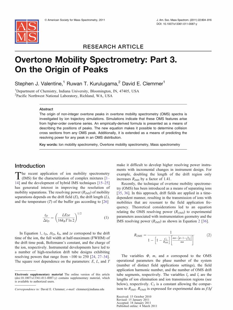
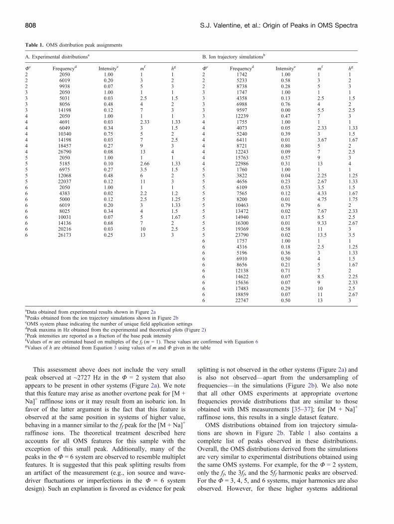
The current algorithm is versatile in that it allowsdifferent OMS phase systems to be examined. Figure 1shows a schematic of the OMS device used for the iontrajectory simulations and a cartoon diagram of the initialion placement in the OMS device with the field arraysettings for different phase systems. A Φ = 2 systemrequires two field arrays, including one in which the odd-numbered (1, 3, 5, etc.) de regions contain fields that willtransmit ions; the remaining, even-numbered de regionscontain fields that will cause the elimination of ions. Forthe second field array, the transmission and elimination(de) regions are reversed. Initially, the algorithm selectsone field array and reads in a region (4 field array points)that surrounds the two-dimensional position of the ion forwhich the calculation is being performed. A weighted-average field is then calculated for both dimensions basedon the distance of the ion to the field values provided ateach surrounding array point. The displacement due to theion mobility is then calculated for a user-defined time step(typically ≤2 μs) by multiplying by vD. For thesesimulations, K is taken from an experimentally availablevalue (e.g., the mobility of [M + H]+ bradykinin ions).

To simulate random diffusion in two dimensions, the rootmean square displacement of an ion,

ffiffiffiffir2

p, is converted into

a polar coordinate vector by randomizing a single angle (Q).The y- and z-axis vector components are determinedfrom

ffiffiffiffir2

p·sinQ and

ffiffiffiffir2

p·cosQ, respectively. The diffusion

value is then added to the displacement due to the ionsmobility to provide a net ion displacement for each timeincrement. A total of n=11 segments have been used foreach of the ion trajectory simulations. For the simulations ofthe F = 2 system, the first two dt regions and the first deregion (164 total grid units along the z-axis of the fieldarray) are filled with ions (10 ions at each grid unit). Theconjoining de regions are each 5 grid units wide (i.e., le = 5grid units). A complete analysis for a specific frequencyrequires 1640 separate ion trajectory simulations.

The simulations for the F = 3 system require threediscrete field array files and the first three d region segmentsare filled with ions up to the de(3) region (Figure 1).Therefore, the total number of grid units filled with ions is249. The total number of grid units that are filled with ionsfor the F = 4, F = 5, and F = 6 systems are 334, 419, and504, respectively. Also, the simulations for the F = 4, F = 5,and F = 6 systems require 4, 5, and 6 independent fieldarray files, respectively. For all simulations, the starting

dt(1)

gate 1(80)

gate 2(165)

gate 3(250)

gate 4(335)

gate 5(420)

gate 6(505)

gate 7(590)

lt=80 le=5

gate 8(675)

dt(2) dt(3) dt(4) dt(5) dt(6) dt(7) dt(8)

G1(on) G2(off)

G1(on) G2(off) G3(off)

G1(on) G2(off) G3(off) G4(off)

G1(on) G2(off) G3(off) G4(off) G5(off)

G1(on) G2(off) G3(off) G4(off) G5(off) G6(off)

= 2

= 3

= 4

= 5

= 6

(a)

(b)voltage profiles

Figure 1. (a) Schematic diagram of the OMS device for the ion trajectory simulation. The first eight ion transmission (dt) and ionelimination regions (de) are shown. For these simulations, the OMS device utilized consists of 11 segments. Each segment isdivided into 80 grid units and the conjoining de sections consist of 5 grid units. Ten ions are placed at each grid unit for thesimulation. The number in parenthesis under the gate number corresponds to the starting grid unit for each gate region. (b) Acartoon diagram showing the initial ion placement for ion trajectory simulations using different phase systems. Each simulationis started by turning on the first gate (G1 or first de region), therefore, all the ions placed in the first segment get neutralized atthe fundamental frequency level. Red lines indicate the “sawtooth” voltage profile for the field application depicted with the gatesettings [35–37]. For example, gates (nΦ + 1 where n = 0,1,2,3,…) that show an abrupt change (minimum to maximum value inthe sawtooth profile) are designated as de regions for this field setting indicating the location of ion neutralization. The solid bluelines show the numbers of d regions that are filled by the ion beam prior to initiating ion elimination at G1. This filling size isrelated to values for ROMS as well as intensities of specific OMS dataset features (see text and Figure 4 for details)

806 S.J. Valentine, et al.: Origin of Peaks in OMS Spectra

frequency was 500 Hz and the frequency is stepped by100 Hz for each analysis. Using a maximum frequency of50 kHz, a total of 495 separate analyses for each value of Fhave been performed. Ion intensities at each frequencysetting are determined as the percentage of ions in thesimulation that are transmitted through the entire OMSregion. OMS spectra generated from the ion trajectorysimulations are compared with experimental datasets forwhich the same phase has been employed.

Results and DiscussionDependence of OMS Distribution Peaks on Φ

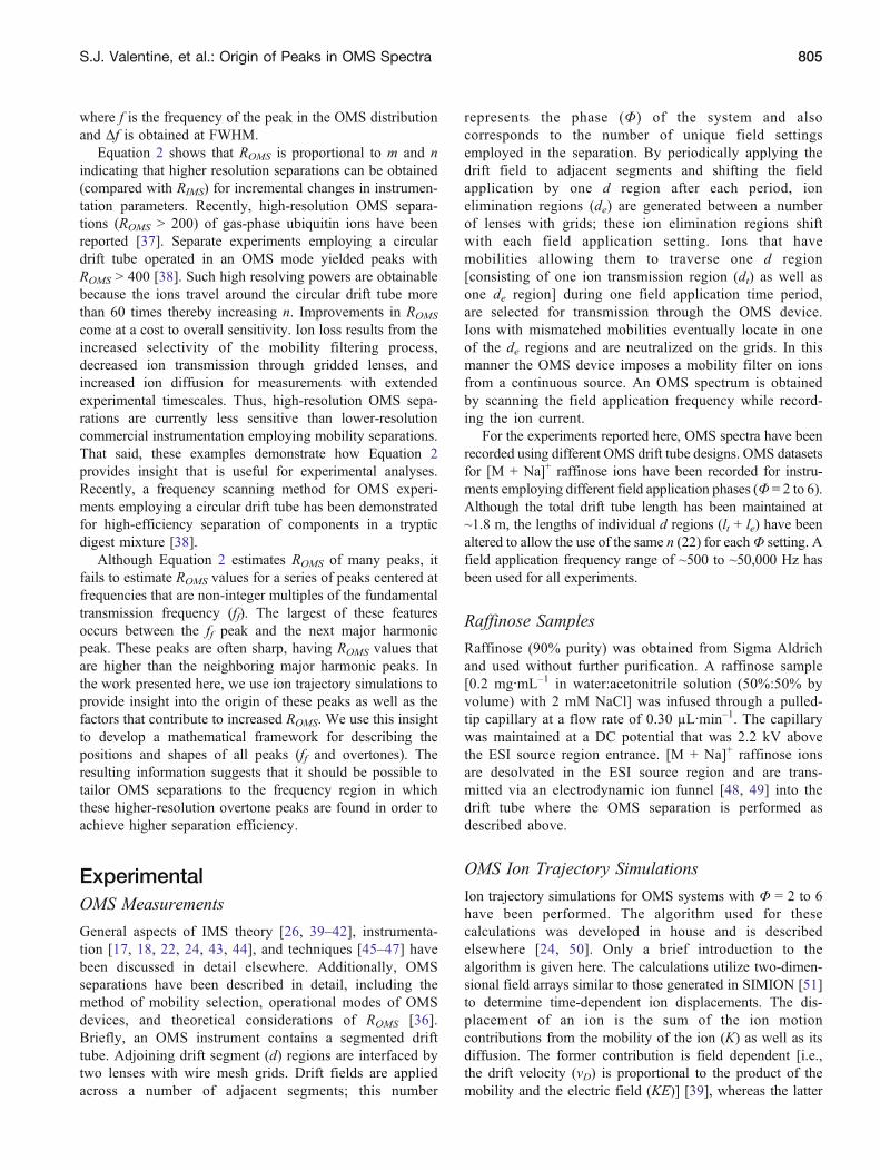
Figure 2a shows OMS spectra recorded for [M + Na]+

raffinose ions for different F values. For F = 2, a feature isobserved at ~2050 Hz corresponding to transmission of the[M + Na]+ raffinose ions at the ff. Two other major featuresare also observed at field application frequencies that are 3and 5 times the ff. Major OMS distribution peaks such asthese have been related to F using m according to therelationship

m ¼ � h� 1ð Þ þ 1 ð3Þ[35, 36]where h corresponds to a harmonic index (h = 1,2,3…).Features in OMS distributions are delineated by theirfrequencies (f) as they relate to the ff according to

f ¼ mff ð4Þ

From the expression for m (Equation 3), major harmonicpeaks in OMS distributions obtained from a Φ = 3 systemwould be centered at ~4ff , ~7ff , ~10ff , etc. Figure 2a showsthe presence of this harmonic series in the OMS spectra for[M + Na]+ raffinose ions collected with a Φ = 3 device.Figure 2a also shows that lower-frequency peaks from themajor harmonics series predicted by m are also observed forthe Φ = 4, the Φ = 5, and the Φ = 6 systems. Peakassignments for the major harmonics series as observed inthe experimental datasets (Figure 2a) are listed in Table 1.

Examination of the OMS spectra for the [M + Na]+

raffinose ions in Figure 2a shows that many other featuresthat cannot be accounted for by values of m (as definedby Equation 3) are present. For the Φ = 4 system, twodistinct features are observed between the ff and the 5ffpeaks. These features have peak centers of 4691 and6049 Hz which are factors of 2.28 and 2.95 times higherthan the ff. It is instructive to consider the resolution ofthese peaks. ROMS values of 47 and 41 have beendetermined for these two features. These values aregreater than those determined for the neighboring majorharmonic peaks (i.e., the peaks centered at ff and 5ff).Peaks located between the first two major harmonic peaksare observed for all systems with the exception of the Φ =

2 system, and the number of peaks in this regionincreases with increasing values of Φ (Figure 2a). Theseexperimental data also show that some additional peaksarise between the second and third major harmonic peaksof the OMS distributions. Examples include peakscentered at ~14198 and ~20216 Hz for the Φ = 4 andthe Φ = 6 systems, respectively. These peak centers arefactors of 6.92 and 9.86 higher than the ff, which are alsonot predicted by integer values of m according toEquation 4. These overtone peaks all have ROMS valuesexceeding those of neighboring major harmonic peaks.These overtone peaks (not described previously) withassociated peak intensities are also listed in Table 1.

= 2

= 3

= 4

= 5

= 6

ff3ff 5ff

4ff 7ff

5ff 9ff 13ff

6ff11ff

7ff13ff

= 2

= 3

= 4

= 5

= 6

ff

3ff 5ff

4ff7ff

5ff9ff 13ff

6ff11ff

7ff13ff

Field application frequency (Hz)

Inte

nsity

(ar

bitr

ary

units

)In

tens

ity (

arbi

trar

y un

its)

(b)

(a)

Figure 2. (a) OMS distributions obtained for [M + Na] +raffinose ions using OMS devices employing Φ = 2 to 6systems. Peaks in the primary harmonic series (see text fordiscussion) are labeled for each system. For these studies,the OMS drift tube is ~1.8 m long and a buffer gas pressureand drift field of ~3 Torr and 10 V·cm–1 have been used. TheOMS region of the drift tube is ~1.2 Torr and a total numberof 22 d regions have been employed for each system. b)OMS spectra obtained using ion trajectory simulations forOMS devices employing Φ = 2 to 6 systems. Ion trajectorysimulations are carried out using an algorithm developed inhouse (see text for details). Peaks in the primary harmonicseries are labeled for each system. For this virtual OMSdevice, 11 d regions have been employed. A model mobilityof 0.09 m2·V–1·s–1 has been used for all ions in thesimulations described here


This assessment above does not include the very smallpeak observed at ~2727 Hz in the Φ = 2 system that alsoappears to be present in other systems (Figure 2a). We notethat this feature may arise as another overtone peak for [M +Na]+ raffinose ions or it may result from an isobaric ion. Infavor of the latter argument is the fact that this feature isobserved at the same position in systems of higher value,behaving in a manner similar to the ff peak for the [M + Na]+

raffinose ions. The theoretical treatment described hereaccounts for all OMS features for this sample with theexception of this small peak. Additionally, many of thepeaks in the Φ = 6 system are observed to resemble multipletfeatures. It is suggested that this peak splitting results froman artifact of the measurement (e.g., ion source and wave-driver fluctuations or imperfections in the Φ = 6 systemdesign). Such an explanation is favored as evidence for peak

splitting is not observed in the other systems (Figure 2a) andis also not observed—apart from the undersampling offrequencies—in the simulations (Figure 2b). We also notethat all other OMS experiments at appropriate overtonefrequencies provide distributions that are similar to thoseobtained with IMS measurements [35–37]; for [M + Na]+

raffinose ions, this results in a single dataset feature.OMS distributions obtained from ion trajectory simula-

tions are shown in Figure 2b. Table 1 also contains acomplete list of peaks observed in these distributions.Overall, the OMS distributions derived from the simulationsare very similar to experimental distributions obtained usingthe same OMS systems. For example, for the Φ = 2 system,only the ff, the 3ff, and the 5ff harmonic peaks are observed.For the Φ = 3, 4, 5, and 6 systems, major harmonics are alsoobserved. However, for these higher systems additional

Table 1. OMS distribution peak assignments

A. Experimental distributionsa B. Ion trajectory simulationsb

Φc Frequencyd Intensitye mf hg Φc Frequencyd Intensitye mf hg

2 2050 1.00 1 1 2 1742 1.00 1 12 6019 0.20 3 2 2 5233 0.58 3 22 9938 0.07 5 3 2 8738 0.28 5 33 2050 1.00 1 1 3 1747 1.00 1 13 5031 0.03 2.5 1.5 3 4358 0.13 2.5 1.53 8056 0.48 4 2 3 6988 0.76 4 23 14198 0.12 7 3 3 9597 0.00 5.5 2.54 2050 1.00 1 1 3 12239 0.47 7 34 4691 0.03 2.33 1.33 4 1755 1.00 1 14 6049 0.34 3 1.5 4 4073 0.05 2.33 1.334 10340 0.75 5 2 4 5240 0.39 3 1.54 14198 0.03 7 2.5 4 6411 0.01 3.67 1.674 18457 0.27 9 3 4 8721 0.80 5 24 26790 0.08 13 4 4 12243 0.09 7 2.55 2050 1.00 1 1 4 15763 0.57 9 35 5185 0.10 2.66 1.33 4 22986 0.31 13 45 6975 0.27 3.5 1.5 5 1760 1.00 1 15 12068 0.48 6 2 5 3822 0.04 2.25 1.255 22037 0.12 11 3 5 4656 0.23 2.67 1.336 2050 1.00 1 1 5 6109 0.53 3.5 1.56 4383 0.02 2.2 1.2 5 7565 0.12 4.33 1.676 5000 0.12 2.5 1.25 5 8200 0.01 4.75 1.756 6019 0.20 3 1.33 5 10463 0.79 6 26 8025 0.34 4 1.5 5 13472 0.02 7.67 2.336 10031 0.07 5 1.67 5 14940 0.17 8.5 2.56 14136 0.68 7 2 5 16300 0.01 9.33 2.676 20216 0.03 10 2.5 5 19369 0.58 11 36 26173 0.25 13 3 5 23790 0.02 13.5 3.5

6 1757 1.00 1 16 4316 0.18 2.5 1.256 5196 0.36 3 1.336 6910 0.50 4 1.56 8656 0.21 5 1.676 12138 0.71 7 26 14622 0.07 8.5 2.256 15636 0.07 9 2.336 17483 0.29 10 2.56 18859 0.07 11 2.676 22747 0.50 13 3

aData obtained from experimental results shown in Figure 2abPeaks obtained from the ion trajectory simulations shown in Figure 2bcOMS system phase indicating the number of unique field application settingsdPeak maxima in Hz obtained from the experimental and theoretical plots (Figure 2)ePeak intensities are reported as a fraction of the base peak intensityfValues of m are estimated based on multiples of the ff (m = 1). These values are confirmed with Equation 6gValues of h are obtained from Equation 3 using values of m and Φ given in the table


peaks are observed between the major harmonic peaksexhibiting overtones matching those observed experimen-tally. The relative peak intensities of the different peaks arealso similar to the experimental results. For all systems, peakintensities decrease with increasing frequency within themajor harmonic peak series. Conversely, in general, peakintensities increase with increasing frequency for the over-tone peaks observed between the major harmonic peaks.

It is instructive to consider a single system in greaterdetail in order to obtain a general description of peaksobserved in OMS experiments. The Φ = 4 system generatedfour primary harmonic peaks (Figure 2b) centered at 1755,8721, 15,763, and 22,986 Hz and four more low intensitypeaks centered at 4073, 5240, 6411, and 12,243 Hz. Thefour primary harmonic peaks correspond to those observedat the ff, 5ff, 9ff, and 13ff field application frequencies,respectively, and are predicted for the Φ = 4 system byEquation 3. The respective intensities for the majorharmonic peaks are 70, 56, 40, and 22. The minor overtonepeaks are located at ~2.3ff, ~3ff, ~3.6ff, and ~7ff, respectively.The intensities for the minor overtone peaks (in order ofincreasing frequency) are 3.8, 27, 0.7, and 6.2.

Although, the OMS spectra obtained from the ion trajectorysimulations resemble those obtained experimentally for [M +Na]+ raffinose, several differences are observed. OMS peaksare more highly resolved in the experimental datasets. This isdue to the use of an instrument with 22 segments whereas theion trajectory simulations employed a model device with 11segments [35, 36]. Although the primary harmonic peaksobserved for the experimental data are essentially the same asthe simulation data, the peak centers are shifted slightly due todifferences in the mobilities of raffinose and the theoretical ionused in the simulations. Although the OMS spectra obtainedfor the Φ = 3, Φ = 4, and Φ = 5 systems show minor peakscentered at similar overtone values compared with theexperimental data, a greater number of minor overtone peaksis observed for the simulation data. For example, for a Φ = 5system, four and two peaks are observed between the first twomajor harmonic peaks for the simulation and the experimentaldata, respectively. Finally, it is noted that a greater degree ofion transmission is observed for the ion trajectory simulations.Most likely this is a result of the fewer gates used in the iontrajectory simulations resulting in fewer ions lost due todiffusion. Additionally, the simulations are carried out in anideal environment and do not account for perturbations inexperimental conditions such as the presence of fringing fieldsthat may affect the transmission of ions in the OMS drift tube.

The peak profile for the Φ = 6 system obtained for [M +Na]+ raffinose ions is significantly different from the dataobtained using the ion trajectory simulations. This isprimarily due to the low-resolution OMS spectrum obtainedfor the computer simulation. The baseline for the simulationis not zero at any point (Figure 2b), indicating that ions leakthrough the virtual OMS device. This is likely due to the useof an insufficient n; that is, a larger number of d regionsegments would result in increased OMS separation effi-

ciency as reported earlier and predicted by Equation 2 [36].This also suggests that there is a minimum number of dregions required to prevent ion leakage. Below we relate theselectivity of OMS devices to their ability to segment thecontinuous ion beam into discrete, transmittable packets ofions. Large transmission packets generated by the Φ = 6system result in less discrimination of ions based onmobilities (see discussion below). Selectivity can beincreased by introducing more d regions as observedpreviously in OMS experiments [35–37]; the greater numberof d regions more effectively divides the continuous ionbeam (see discussion below and supplementary informa-tion). Thus, ion trajectory simulations employing a greater nwould produce distributions that are more similar to theexperimental datasets.

Generation of ff Peaks in OMS Distributions

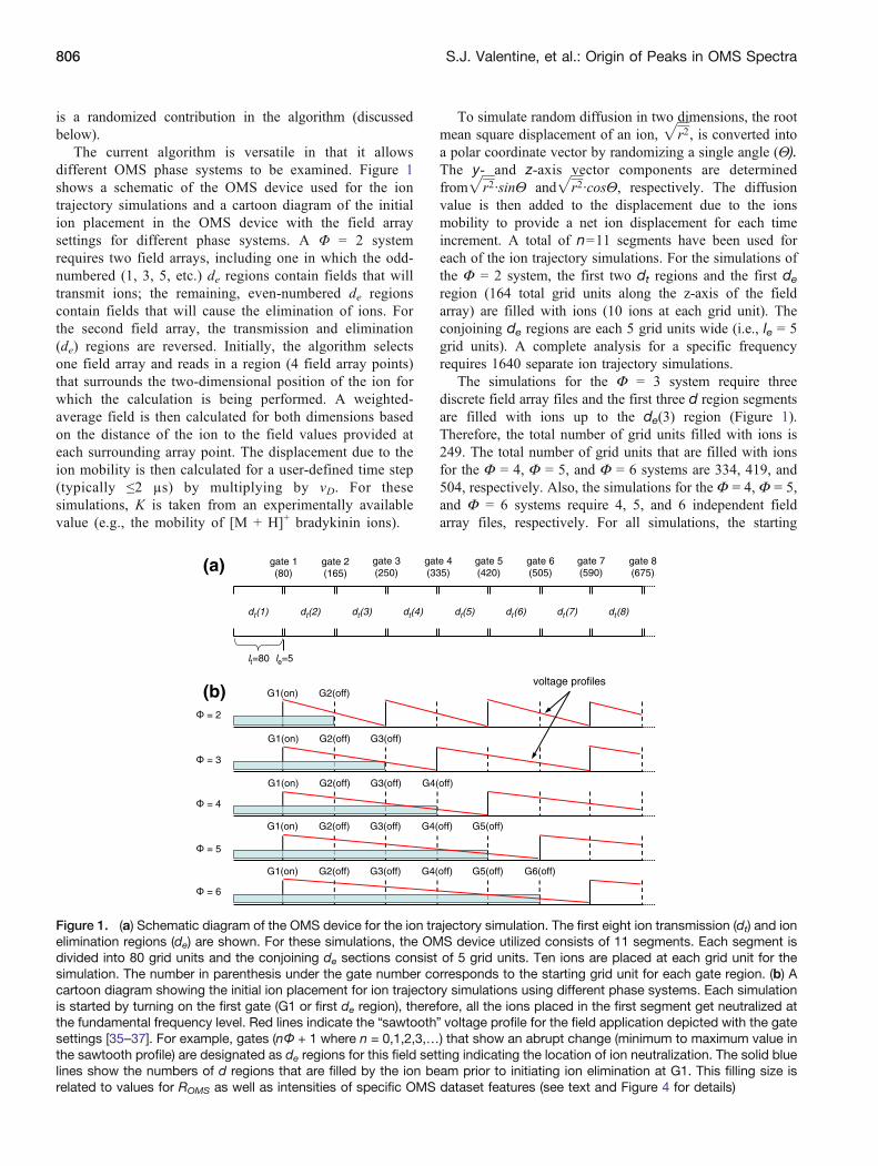
During the course of an OMS separation, the continuous ionbeam is divided into whole regions that are either trans-mitted through the drift tube or eliminated due to theapplication of alternating field settings in the segmented drifttube [36]. Figure 3 shows the distance traversed (final gridnumber) by ions at different starting positions (initial gridnumber) in the ion trajectory simulations for the Φ = 2, 3, 5,and 6 systems. Simulations are carried out using a fieldapplication frequency representing maximum ion transmis-sion (i.e., the ff, which ranges from ~1700 to ~1750 for thesesystems). Figure 3 shows which ions (with respect to initialposition) are neutralized and which pass through the OMSdevice. The grid number values provided on the y axis canbe related to the gate numbers given in Figure 1 to providelocations for ion neutralization events. The last grid number,1015, corresponds to gate 12. Ions that reach gate 12, havepassed through the OMS device unaffected. For example,the plot for Φ = 2 shows that all the ions up to a starting gridnumber of 85 have been neutralized at some point within theOMS device while almost all the ions starting after gridnumber 85 propagate through the OMS region.

It is instructive to consider the starting positions of ionsthat are neutralized on grids after the initial gates. For allsystems these ions are those that are located closer to theedges of the transmitted portion of the ion beam. Forexample, the transmission plot for the Φ = 2 system inFigure 3 shows that the ion transmission region extendsfrom ~85 to ~165 grid units. However, ion losses areobserved to occur on the edges of this transmission regionfrom ~85 to ~100 and from ~152 to ~160 grid units. Ion lossoccurs because of the diffusion of ions into the de regionsduring the simulation. The Φ = 2 system shows a duty cycleof ~50%; that is, neglecting the ions lost due to diffusion,roughly half of the initial ion population reaches the endgate. Simulations show that this 50% duty cycle is true evenfor overtone peaks in the Φ = 2 system. Plots for the Φ = 3,Φ = 5, and Φ = 6 systems (Figure 2) show duty cycles of66%, 80%, and 83%, respectively. Examination of these data


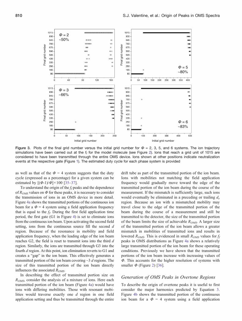
as well as that of the Φ = 4 system suggests that the dutycycle (expressed as a percentage) for a given system can beestimated by [(Φ-1)/Φ]×100 [35–37].

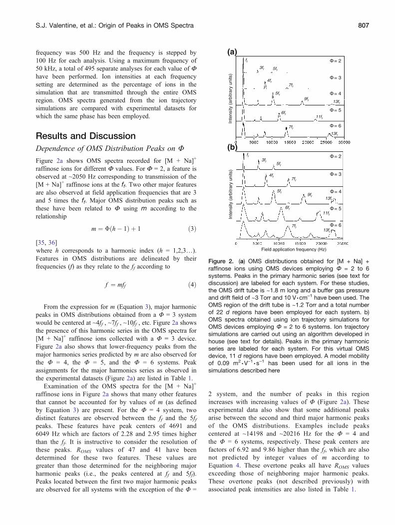
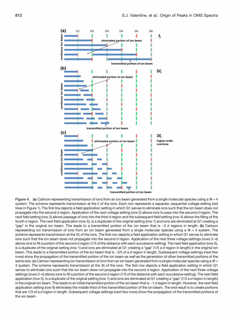
To understand the origin of the ff peaks and the dependenceof ROMS values onΦ for these peaks, it is necessary to considerthe transmission of ions in an OMS device in more detail.Figure 4a shows the transmitted portions of the continuous ionbeam for a Φ = 4 system using a field application frequencythat is equal to the ff. During the first field application timeperiod, the first gate (G1 in Figure 4) is set to eliminate ionsfrom the continuous ion beam. Upon activating the second fieldsetting, ions from the continuous source fill the second dregion. Because of the resonance in mobility and fieldapplication frequency, when the leading edge of the ion beamreaches G2, the field is reset to transmit ions into the third dregion. Similarly, the ions are transmitted through G3 into thefourth d region. At this point, ion elimination reverts to G1 andcreates a “gap” in the ion beam. This effectively generates atransmitted portion of the ion beam covering ~3 d regions. Thesize of this transmitted portion of the ion beam directlyinfluences the associated ROMS.

In describing the effect of transmitted portion size onROMS, consider the analysis of a mixture of ions. Here eachtransmitted portion of the ion beam (Figure 4a) would haveions with differing mobilities. Those with resonant mobi-lities would traverse exactly one d region in one fieldapplication setting and thus be transmitted through the entire

drift tube as part of the transmitted portion of the ion beam.Ions with mobilities not matching the field applicationfrequency would gradually move toward the edge of thetransmitted portion of the ion beam during the course of themeasurement. If the mismatch is sufficiently large, such ionswould eventually be eliminated in a preceding or trailing deregion. Because an ion with a mismatched mobility maytravel close to the edge of the transmitted portion of thebeam during the course of a measurement and still betransmitted to the detector, the size of the transmitted portionof the beam limits the size of achievable ROMS. A larger sizeof the transmitted portion of the ion beam allows a greatermismatch in mobilities of transmitted ions and results inlowered ROMS. This is evidenced in small ROMS values for ffpeaks in OMS distributions as Figure 4a shows a relativelylarge transmitted portion of the ion beam for these operatingconditions. Previously we have shown that the transmittedportions of the ion beam increase with increasing values ofΦ. This accounts for the higher resolution of systems withsmaller Φ (Figure 2) [36].

Generation of OMS Peaks in Overtone Regions

To describe the origin of overtone peaks it is useful to firstconsider the major harmonics predicted by Equation 3.Figure 4b shows the transmitted portion of the continuousion beam for a Φ = 4 system using a field application

Initial grid number Initial grid number

= 2~50%

= 3~66%

= 6~83%

= 5~80%

Fin

al g

rid n

umbe

rF

inal

grid

num

ber

Fin

al g

rid n

umbe

rF

inal

grid

num

ber

Figure 3. Plots of the final grid number versus the initial grid number for Φ = 2, 3, 5, and 6 systems. The ion trajectorysimulations have been carried out at the ff for the model molecule (see Figure 2). Ions that reach a grid unit of 1015 areconsidered to have been transmitted through the entire OMS device. Ions shown at other positions indicate neutralizationevents at the respective gate (Figure 1). The estimated duty cycle for each phase system is provided


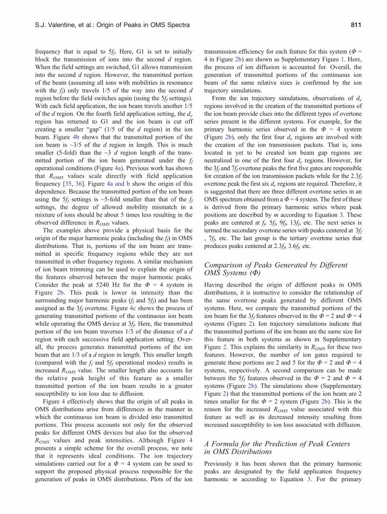
frequency that is equal to 5ff. Here, G1 is set to initiallyblock the transmission of ions into the second d region.When the field settings are switched, G1 allows transmissioninto the second d region. However, the transmitted portionof the beam (assuming all ions with mobilities in resonancewith the ff) only travels 1/5 of the way into the second dregion before the field switches again (using the 5ff settings).With each field application, the ion beam travels another 1/5of the d region. On the fourth field application setting, the deregion has returned to G1 and the ion beam is cut offcreating a smaller “gap” (1/5 of the d region) in the ionbeam. Figure 4b shows that the transmitted portion of theion beam is ~3/5 of the d region in length. This is muchsmaller (5-fold) than the ~3 d region length of the trans-mitted portion of the ion beam generated under the ffoperational conditions (Figure 4a). Previous work has shownthat ROMS values scale directly with field applicationfrequency [35, 36]. Figure 4a and b show the origin of thisdependence. Because the transmitted portion of the ion beamusing the 5ff settings is ~5-fold smaller than that of the ffsettings, the degree of allowed mobility mismatch in amixture of ions should be about 5 times less resulting in theobserved difference in ROMS values.

The examples above provide a physical basis for theorigin of the major harmonic peaks (including the ff) in OMSdistributions. That is, portions of the ion beam are trans-mitted in specific frequency regions while they are nottransmitted in other frequency regions. A similar mechanismof ion beam trimming can be used to explain the origin ofthe features observed between the major harmonic peaks.Consider the peak at 5240 Hz for the Φ = 4 system inFigure 2b. This peak is lower in intensity than thesurrounding major harmonic peaks (ff and 5ff) and has beenassigned as the 3ff overtone. Figure 4c shows the process ofgenerating transmitted portions of the continuous ion beamwhile operating the OMS device at 3ff. Here, the transmittedportion of the ion beam traverses 1/3 of the distance of a dregion with each successive field application setting. Over-all, the process generates transmitted portions of the ionbeam that are 1/3 of a d region in length. This smaller length(compared with the ff and 5ff operational modes) results inincreased ROMS value. The smaller length also accounts forthe relative peak height of this feature as a smallertransmitted portion of the ion beam results in a greatersusceptibility to ion loss due to diffusion.

Figure 4 effectively shows that the origin of all peaks inOMS distributions arise from differences in the manner inwhich the continuous ion beam is divided into transmittedportions. This process accounts not only for the observedpeaks for different OMS devices but also for the observedROMS values and peak intensities. Although Figure 4presents a simple scheme for the overall process, we notethat it represents ideal conditions. The ion trajectorysimulations carried out for a Φ = 4 system can be used tosupport the proposed physical process responsible for thegeneration of peaks in OMS distributions. Plots of the ion

transmission efficiency for each feature for this system (Φ =4 in Figure 2b) are shown as Supplementary Figure 1. Here,the process of ion diffusion is accounted for. Overall, thegeneration of transmitted portions of the continuous ionbeam of the same relative sizes is confirmed by the iontrajectory simulations.

From the ion trajectory simulations, observations of deregions involved in the creation of the transmitted portions ofthe ion beam provide clues into the different types of overtoneseries present in the different systems. For example, for theprimary harmonic series observed in the Φ = 4 system(Figure 2b), only the first four de regions are involved withthe creation of the ion transmission packets. That is, ionslocated in yet to be created ion beam gap regions areneutralized in one of the first four de regions. However, forthe 3ff and 7ff overtone peaks the first five gates are responsiblefor creation of the ion transmission packets while for the 2.3ffovertone peak the first six de regions are required. Therefore, itis suggested that there are three different overtone series in anOMS spectrum obtained from aΦ = 4 system. The first of theseis derived from the primary harmonic series where peakpositions are described by m according to Equation 3. Thesepeaks are centered at ff, 5ff, 9ff, 13ff, etc. The next series istermed the secondary overtone series with peaks centered at 3ff, 7ff, etc. The last group is the tertiary overtone series thatproduces peaks centered at 2.3ff, 3.6ff, etc.

Comparison of Peaks Generated by DifferentOMS Systems (Φ)

Having described the origin of different peaks in OMSdistributions, it is instructive to consider the relationship ofthe same overtone peaks generated by different OMSsystems. Here, we compare the transmitted portions of theion beam for the 3ff features observed in the Φ = 2 and Φ = 4systems (Figure 2). Ion trajectory simulations indicate thatthe transmitted portions of the ion beam are the same size forthis feature in both systems as shown in SupplementaryFigure 2. This explains the similarity in ROMS for these twofeatures. However, the number of ion gates required togenerate these portions are 2 and 5 for the Φ = 2 and Φ = 4systems, respectively. A second comparison can be madebetween the 5ff features observed in the Φ = 2 and Φ = 4systems (Figure 2b). The simulations show (SupplementaryFigure 2) that the transmitted portions of the ion beam are 2times smaller for the Φ = 2 system (Figure 2b). This is thereason for the increased ROMS value associated with thisfeature as well as its decreased intensity resulting fromincreased susceptibility to ion loss associated with diffusion.

A Formula for the Prediction of Peak Centersin OMS Distributions

Previously it has been shown that the primary harmonicpeaks are designated by the field application frequencyharmonic m according to Equation 3. For the primary


ff

5ff

3ffhigher-orderovertone

con

tin

ou

s io

n b

eam

con

tin

ou

s io

n b

eam

con

tin

ou

s io

n b

eam

transmitted portion of ion beam



(a)

(b)

(c)

G1 G2 G3 G4 G5 G6

eliminated portion of ion beam



Figure 4. (a) Cartoon representing transmission of ions from an ion beam generated from a single molecular species using aΦ = 4system. The scheme represents transmission at the ff of the ions. Each row represents a separate, sequential voltage setting (redlines in Figure 1). The first line depicts a field application setting in which G1 serves to eliminate ions such that the ion beam does notpropagate into the second d region. Application of the next voltage setting (row 2) allows ions to pass into the second d region. Thenext field setting (row 3) allows passage of ions into the third d region and the subsequent field setting (row 4) allows the filling of thefourth d region. The next field application (row 5), is a duplicate of the original setting (row 1) and ions are eliminated at G1 creating a“gap” in the original ion beam. This leads to a transmitted portion of the ion beam that is ~3 d regions in length. (b) Cartoonrepresenting ion transmission of ions from an ion beam generated from a single molecular species using a Φ = 4 system. Thescheme represents transmission at the 5ff of the ions. The first row depicts a field application setting in which G1 serves to eliminateions such that the ion beam does not propagate into the second d region. Application of the next three voltage settings (rows 2–4)allows ions to fill a portion of the second d region (1/5 of the distance with each successive setting). The next field application (row 5),is a duplicate of the original setting (row 1) and ions are eliminated at G1 creating a “gap” (1/5 a d region in length) in the original ionbeam. This leads to a transmitted portion of the ion beam that is ~3/5 of a d region in length. Subsequent voltage settings (next fewrows) show the propagation of the transmitted portion of the ion beam as well as the generation of other transmitted portions of thesame size. (c) Cartoon representing ion transmission of ions from an ion beamgenerated from a singlemolecular species using aΦ =4 system. The scheme represents transmission at the 3ff of the ions. The first row depicts a field application setting in which G1serves to eliminate ions such that the ion beam does not propagate into the second d region. Application of the next three voltagesettings (rows 2–4) allows ions to fill a portion of the second d region (1/3 of the distancewith each successive setting). The next fieldapplication (row 5), is a duplicate of the original setting (row 1) and ions are eliminated at G1 creating a “gap” (1/3 a d region in length)in the original ion beam. This leads to an initial transmitted portion of the ion beam that is ~1d region in length. However, the next fieldapplication setting (row 6) eliminates the middle third of this transmitted portion of the ion beam. The end result is to create portionsthat are 1/3 of a d region in length. Subsequent voltage settings (next few rows) show the propagation of the transmitted portions ofthe ion beam


harmonic series within all systems, h varies as 1, 2, 3,…etc.However, separate calculations are required to describe theother overtone series (hereafter described as higher-orderovertones). These can be obtained from the estimated valuesof m for these higher-order overtones listed in Table 1. Forexample, for the secondary overtone series, h must vary as1.5, 2, 2.5,…etc., and for the tertiary overtone series, h mustvary as 1.33, 1.67, 2,…etc. The secondary overtone series isobserved for systems where Φ ≥ 3 and the tertiary overtoneseries is observed for systems where Φ ≥ 4 (Table 1). For aΦ = 5 system, in addition to the above overtone series,another series with h varying as 1.25, 1.5, 1.75,…etc, exists.Similarly, for the Φ = 6 system, in addition to the overtoneseries described above, there is another series with h varyingas 1.2, 1.4, 1.6, 1.8,…etc.

The empirically-derived equation accounting for thehigher order overtone series is,

h ¼ q

f� k

� �þ 1 ð5Þ

In Equation 5, the variable k (overtone series index) haslimits of 0 to Φ – 1, and the variable q (overtone peak index)has limits of 0 → ∞. Equations 3 and 5 can be combined toprovide a complete index of frequencies (m) for all OMSdataset features according to

m ¼ fq

f� k

� �þ 1 ð6Þ

Here m no longer corresponds to true harmonics (i.e.,integer multiples of the ff). Thus the new term for m is OMSfrequency coefficient.

Determining Ion Collision Cross Sectionsfrom OMS Peaks

Previously, an equation has been reported that allows thedetermination of collision cross sections using the fieldapplication frequencies of the major harmonic peaks [36].Calculations of collision cross section using OMS data havepreviously been shown to be very accurate as valuesobtained from OMS datasets have been determined to bewithin ±1% of established values determined by IMSmeasurements [37]. It is possible to incorporate the variablem into the collision cross section equation to obtain theexpression,

� ¼ 18pð Þ1=216

ze

kbTð Þ1=21

mIþ 1

mB

� �1=2 Em

f lt þ leð Þ760

P

� T

273:2

1

Nð7Þ

In Equation 7, the variables mI and mB correspond to themasses of the ion and the buffer gas, respectively. Thevariables T, P, and N correspond to the temperature, thepressure, and the neutral number density at STP of the buffergas, respectively. Finally, f corresponds to the frequency ofthe peak used for the calculation.

One advantage of Equation 7 is that it allows thedetermination of collision cross section from any peak inthe OMS dataset; previously this calculation was only validfor primary harmonic peaks. For sample mixtures, OMSspectra can be examined for spectral regions containinglimited interference from chemical noise in order to obtain acollision cross section measurement. Additionally, the multi-ple measurements obtained from the various overtone peakscan serve to confirm collision cross section calculations inorder to increase the accuracy of the determination.

A disadvantage of the cross section calculation is that itrequires a knowledge of the value of m in order to performthe calculation which can be problematic for samplemixtures. That said, because of the relationship amongfeatures in the different peak series, assignments of m maybe obtained by direct comparison of related peaks. Such aprocess would be very similar to that employed in decipher-ing electrospray ionization (ESI) charge state distributions.Here, a ratio of peak frequencies would be compared to aratio of m values within an overtone series. One advantagefor the OMS approach is that OMS distributions provideeven more distinctive information than ESI charge statedistributions. This information is contained within therelative intensities of the peaks in that specific overtoneseries have characteristic intensities. As described in detailabove, these intensities are related to the size of thetransmitted portion of the ion beam at a given frequencyand thus ultimately to ROMS. In practice it would berelatively straightforward to determine target OMS regionsbased on the characteristic mobilities of mixture compo-nents.9 From there the determination of peak ratios can beperformed; as evident in Figure 2, determining features thatbelong to the same overtone series which are candidates forthe ratio comparison is a straightforward process.

Predicting ROMS for OMS Distribution Peaks

With an expression describing the frequencies for all expectedpeaks in OMS distributions, a question arises as to whether ornot ROMS can be predicted for peaks of different overtoneseries. Peak widths in OMS distributions indicate thatEquation 6 cannot be substituted directly into Equation 2 asthis does not capture the fact that ROMS values for peaks inhigher-order overtone series are larger than those of neighbor-ing primary harmonic peaks. For example, from ion trajectorysimulations of theΦ = 4 system (Figure 2b), the peaks centeredat ff and 5ff have ROMS values of 3.4 and 14, respectively. Thefirst observable peaks in the higher-order overtone series at~2.33ff and ~3ff have ROMS values of 30 and 20, respectively.Thus, although ROMS increases with increasing frequency for


the primary harmonic series, for the higher-order overtoneseries, it decreases with increasing frequency. This is only truefor higher-order overtone peaks that have the same value of q(Equation 6). For example, a q-value of 1 is determined for thepeaks at ~2.33ff and ~3ff (Figure 2b). A low-intensity peakcentered at ~3.67ff is also located between the ff peak and the 5ffpeak. This peak however has a ROMS value of ~50. Thedifference is that a different q value (2 in this case) describesthis peak position according to Equation 6.

An observation that helps to yield an expression for ROMS

for higher-order overtone series peaks is that the ratios of ROMS

values for the peak of interest and the major harmonic peakwith the same q value can be related by the fraction Φ/(k + 1)where k is given as the value used to calculate the position ofthe peak of interest. For example, for the ion trajectorysimulations of the Φ = 4 system, the peaks centered at 2.33ff(q =1, k=1) and 5ff (q=1, k=3) have ROMS values of 30 and 14,respectively. The ratio of ROMS values is 2.14 (30/14). Using avalue of k=1 for the peak centered at 2.33ff, a similar value of2.0 is obtained for the fraction Φ/(k + 1). This correlationbetween ROMS ratios and the fraction Φ/(k + 1) is verified forother peaks in higher-order overtone series. For example, theROMS ratio for the peak centered at 3ff (q=1, k=2) and the peakcentered at 5ff (q=1, k=3) is 1.36. The fractionΦ/(k + 1) for thepeak centered at 3ff is 1.33. This relationship also holds forOMS peaks in higher-order overtone series where q is greaterthan 1. For example, the ROMS ratio for the peak centered at3.67ff (q=2, k=1) and the peak centered at 9ff (q=2, k=3) is2.13. The fraction Φ/(k + 1) for the peak centered at 3.67ff is2.00. Thus, it is suggested that Equation 2 can be modified toprovide the ROMS value for major harmonic peaks at a given qvalue. The resulting equation can then be multiplied by thefraction Φ/(k + 1) to obtain the resolving power of any peak inan OMS distribution. The new ROMS equation becomes

ROMS ¼ 1

1� 1� C2RIMS

h ifqþ1½ �n� f�1� le

ltþle½ �fqþ1½ �n

� � fk þ 1

ð8Þ

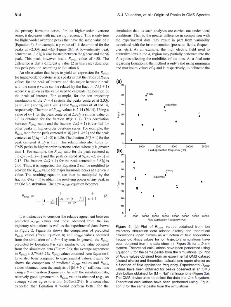
It is instructive to consider the relative agreement betweenpredicted ROMS values and those obtained from the iontrajectory simulations as well as the experimental data shownin Figure 2. Figure 5a shows the comparison of predictedROMS values (from Equation 8) and ROMS values obtainedfrom the simulation of a Φ = 4 system. In general, the ROMS

predicted by Equation 8 is very similar to the value obtainedfrom the simulation data (Figure 2b); the average agreementin ROMS is 5.7%±3.2%. ROMS values obtained fromEquation 8have also been compared to experimental values. Figure 5bshows the comparison of predicted ROMS values and ROMS

values obtained from the analysis of [M + Na]+ raffinose ionsusing a Φ = 6 system (Figure 2a). As with the simulation data,relatively good agreement in ROMS value is obtained (e.g., onaverage values agree to within 6.0%±5.2%). It is somewhatexpected that Equation 8 would perform better for the

simulation data as such analyses are carried out under idealconditions. That is, the greater difference in comparison withthe experimental data may result in part from variabilityassociated with the instrumentation (pressure, fields, frequen-cies, etc.). As an example, the high electric field used toneutralize ions in the de region may partially penetrate into thedt regions affecting the mobilities of the ions. As a final noteregarding Equation 8, the method is only valid using minimumand maximum values of q and k, respectively, to delineate the

0

10

20

30

40

50

60

0 5000 10000 15000 20000 25000Field application frequency (Hz)

RO

MS

theory

experiment

0

10

20

30

40

50

60

70

80

0 5000 10000 15000 20000 25000 30000 35000 40000Field application frequency (Hz)

RO

MS

theory

experiment

(a)

(b)

Figure 5. (a) Plot of ROMS values obtained from iontrajectory simulation data (closed circles) and theoreticalcalculations (open circles) as a function of field applicationfrequency. ROMS values for ion trajectory simulations havebeen obtained from the data shown in Figure 2b for a Φ = 4system. Theoretical calculations have been performed usingEquation 8 for the same peaks from the simulations. (b) Plotof ROMS values obtained from an experimental OMS dataset(closed circles) and theoretical calculations (open circles) asa function of field application frequency. Experimental ROMS

values have been obtained for peaks observed in an OMSdistribution obtained for [M + Na]+ raffinose ions (Figure 2a).The OMS device used to collect the data is a Φ = 6 system.Theoretical calculations have been performed using Equa-tion 8 for the same peaks from the simulations


specific overtone peaks as multiple combinations of thesevariables can lead to the same m number (Equation 6).

Utilizing the Higher-Order Overtone Region

Because of the high resolving power afforded by the higher-order overtone regions of OMS distributions, it is instructiveto consider practical applications for their use in OMSseparations. First, the knowledge gained from ion trajectorysimulations can be used to devise high-resolution OMSseparations. For example, an OMS instrument with anincreased number of d regions can provide substantiallyhigher resolving power. If n is increased from 22 to 100 tocreate an OMS drift tube that is ~4.5 m long, the predictedROMS value for the first overtone peak (q=1, k=0) locatedbetween the first two major harmonic peaks would be 9450for a Φ = 6 system. The development of such instrumenta-tion for routine analyses may have a significant impact forthe study of complex mixtures containing ions with similarmobilities including mixtures of molecular isomers.

Related instrumental development work may include theincorporation of higher-order overtone region character-ization with a circular drift tube. Recently we have shownthat a circular drift tube can be operated in an OMS mode toprovide a high resolution separation (ROMS 9 400) of mixturecomponents according to differences in mobilities at theresonant ff settings [38]. The current geometry of the circulardrift tube is not conducive to transmission of ions atovertone frequencies because the de region is larger thanthe dt region. However, it would be relatively straightfor-ward to decrease the size of the de region such that overtonefrequencies could be attained. Assuming transmission ofions for 60 3/4 cycles as has been performed previously, atheoretical ROMS 9 1600 could be obtained for the firstovertone peak (q=1, k=0) using a Φ = 6 system.

A separate advantage in using the higher-order overtoneregion of an OMS distribution is that the separation region iscondensed. For example, the higher-order overtone regionfor a Φ = 6 system in which all peaks have a q value of 1extends from 2ff to 4ff. To obtain a similar resolving powerin the major harmonics peak region, it would be necessary toscan the frequency range of the 19ff to the 25ff region.Assuming a ff of 2000 Hz, the frequency range to be scannedin the higher-order overtone series is ~2000 Hz; the rangeincreases to ~12,000 Hz for the major harmonics region.Thus there is an analytical throughput advantage that is quitesignificant. This advantage can be offset by scanning at afaster rate in the higher frequency region (albeit at a loss tooverall ion signal levels) as well as by increasing the stepsize of the field application frequency settings (leading toless resolution than can be achieved with smaller steps). Thatsaid, because of the presence of multiple higher-orderovertone peaks in the higher-order overtone series region, aproblem may arise from chemical noise. However, becauseOMS analyses are in effect measurements of collision crosssections, it would be relatively straightforward to determine

the overtones for interfering peaks and disregard them in theanalysis of the OMS distributions.

Summary and ConclusionIon trajectory simulations have been used to provide anexplanation for the origin of peaks in OMS distributions.Simulations show the origin of a major harmonic series ofpeaks as well as several higher-order overtone series ofpeaks. From the analysis of different OMS systems, anempirically-derived formula is presented that predicts thepeak pattern for any OMS distribution. This formula alsoallows the determination of ion collision cross sections fromany feature within an OMS distribution. Additionally, ananalytical expression has been derived that can be used topredict ROMS values as well as to estimate relative peakintensities for expected features in OMS distributions. Thisinformation should be valuable in the process of construct-ing improved OMS instruments. A unique feature of OMScompared with other mobility-based separation techniques isthe fact that the analysis can be carried out at differentfrequency ranges in order to tailor the type of analysisperformed to the desired separation efficiency.

AcknowledgmentsThe authors are grateful for partial support of this work fromthe National Institutes of Health (1RC1GM090797-01) andthe METACyt initiative, funded by a grant from the LillyEndowment. This work is also supported in part by fundingthrough the DoD NSWC Crane “Next Generation ThreatDetection” (N00164-08-C-JQ11).

References1. Moon, M.H., Myung, S., Plasencia, M., Hilderbrand, A.E., Clemmer,

D.E.: Nanoflow LC/ion mobility/CID/TOF for proteomics: analysis of ahuman urinary proteome. J. Proteome Res. 2, 589–597 (2003)

2. Taraszka, J.A., Kurulugama, R., Sowell, R., Valentine, S.J., Koeniger,S.L., Arnold, R.J., Miller, D.F., Kaufman, T.C., Clemmer, D.E.:Mapping the proteome of drosophila melanogaster: analysis ofembryos and adult heads by LC-IMS-MS methods. J. Proteome Res.4, 1223–1237 (2005)

3. Valentine, S.J., Plasencia, M.D., Liu, X., Krishnan, M., Naylor, S.,Udseth, H.R., Smith, R.D., Clemmer, D.E.: Toward plasma proteomeprofiling with ion mobility-mass spectrometry. J. Proteome Res. 5,2977–2984 (2006)

4. Liu, X., Valentine, S.J., Plasencia, M.D., Trimpin, S., Naylor, S.,Clemmer, D.E.: Mapping the human plasma proteome by SCX-LC-IMS-MS. J. Am. Soc. Mass Spectrom. 18, 1249–1264 (2007)

5. Fenn, L.S., McLean, J.A.: Simultaneous glycoproteomics on the basisof structure using ion mobility-mass spectrometry. Mol. Biosyst. 5(11),1298–1302 (2009)

6. Baker, E.S., Livesay, E.A., Orton, D.J., Moore, R.J., Danielson, W.F.,Prior, D.C., Ibrahim, Y.M., LaMarche, B.L., Mayampurath, A.M.,Schepmoes, A.A., Hopkins, D.F., Tang, K.Q., Smith, R.D., Belov, M.E.: An LC-IMS-MS platform providing increased dynamic range forhigh-throughput proteomic studies. J. Proteome Res. 9(2), 997–1006(2010)

7. Dwivedi, P., Wu, P., Klopsch, S.J., Puzon, G.J., Xun, L., Hill, H.H.:Metabolic profiling by ion mobility mass spectrometry (IMMS).Metabolomics 4(1), 63–80 (2008)

8. Kaplan, K., Dwivedi, P., Davidson, S., Yang, Q., Tso, P., Siems, W.,Hill, H.H.: Monitoring dynamic changes in lymph metabolome of


fasting and fed rats by electrospray ionization-ion mobility massspectrometry (ESI-IMMS). Anal. Chem. 81(19), 7944–7953 (2009)

9. Fenn, L.S., McLean, J.A.: Biomolecular structural separations by ionmobility-mass spectrometry. Anal. Chem. Bioanal. Chem. 39, 905–909(2008)

10. Trimpin, S., Tan, B., Bohrer, B.C., O’Dell, D.K., Merenbloom, S.I.,Pazos, M.X., Clemmer, D.E., Walker, J.M.: Profiling of phospholipidsand related lipid structures using multidimensional ion mobilityspectrometry-mass spectrometry. Int. J. Mass Spectrom. 287, 58–69(2009)

11. Isailovic, D., Kurulugama, R.T., Plasencia, M.D., Stokes, S.T.,Kyselova, Z., Goldman, R., Mechref, Y., Novotny, M.V., Clemmer,D.E.: Profiling of human serum glycans associated with liver cancer andcirrhosis by IMS-MS. J. Proteome Res. 7(3), 1109–1117 (2008)

12. Plasencia, M.D., Isailovic, D., Merenbloom, S.I., Mechref, Y.,Clemmer, D.E.: Resolving and assigning N-linked glycan structuralisomers from ovalbumin by IMS-MS. J. Am. Soc. Mass Spectrom. 19(11), 1706–1715 (2008)

13. Becker, C., Qian, K., Russell, D.H.: Molecular weight distributions ofasphaltenes and deasphaltened oils studied by laser desorption ioniza-tion and ion mobility mass spectrometry. Anal. Chem. 80(22), 8592–8597 (2008)

14. Fernandez-Lima, F.A., Becker, C., McKenna, A.M., Rodgers, R.P.,Marshall, A.G., Russel, D.H.: Petroleum crude oil characterization byIMS-MS and FTICR MS. Anal. Chem. 81(24), 9941–9947 (2009)

15. Liu, Y., Clemmer, D.E.: Characterizing oligosaccharides using injected-ion mobility/mass spectrometry. Anal. Chem. 69, 2504–2509 (1997)

16. Liu, Y., Valentine, S.J., Counterman, A.E., Hoaglund, C.S., Clemmer,D.E.: Injected-ion mobility analysis of biomolecules. Anal. Chem. 69,728A (1997)

17. Hoaglund-Hyzer, C.S., Li, J., Clemmer, D.E.: Mobility labeling forparallel CID of ion mixtures. Anal. Chem. 72, 2737–2740 (2000)

18. Gillig, K.J., Ruotolo, B., Stone, E.G., Russell, D.H., Fuhrer, K., Gonin,M., Schultz, A.J.: Coupling high-pressure MALDI with ion mobility/orthogonal time-of flight mass spectrometry. Anal. Chem. 72, 3965–3971 (2000)

19. Valentine, S.J., Kulchania, M., Srebalus Barnes, C.A., Clemmer, D.E.:Multidimensional separations of complex peptide mixtures: a combinedhigh-performance liquid chromatography/ion mobility/time-of-flightmass spectrometry approach. Int. J. Mass Spectrom. 212, 97–109(2001)

20. Srebalus Barnes, C.A., Hilderbrand, A.E., Valentine, S.J., Clemmer, D.E.: Resolving isomeric peptide mixtures: a combined HPLC/ionmobility-TOFMS analysis of a 4000-component combinatorial library.Anal. Chem. 74, 26–36 (2002)

21. Valentine, S.J., Koeniger, S.L., Clemmer, D.E.: A split-field drift tubefor separation and efficient fragmentation of biomolecular ions. Anal.Chem. 75, 6202–6208 (2003)

22. Tang, K., Shvartsburg, A.A., Lee, H.N., Prior, D.C., Buschbach, M.A., Li,F.M., Tolmachev, A.V., Anderson, G.A., Smith, R.D.: High-sensitivity ionmobility spectrometry/mass spectrometry using electrodynamic ion funnelinterfaces. Anal. Chem. 77, 3330–3339 (2005)

23. Tang, K.Q., Li, F.M., Shvartsburg, A.A., Strittmatter, E.F., Smith, R.D.:Two-dimensional gas-phase separations coupled to mass spectrometryfor analysis of complex mixtures. Anal. Chem. 77(19), 6381–6388(2005)

24. Koeniger, S.L., Merenbloom, S.I., Valentine, S.J., Jarrold, M.F.,Udseth, H.R., Smith, R.D., Clemmer, D.E.: An IMS-IMS analogue ofMS-MS. Anal. Chem. 78, 4161–4174 (2006)

25. Merenbloom, S.I., Koeniger, S.L., Bohrer, B.C., Valentine, S.J.,Clemmer, D.E.: Improving the efficiency of IMS-IMS by a combingtechnique. Anal. Chem. 80(6), 1918–1927 (2008)

26. Revercomb, H.W., Mason, E.A.: Theory of plasma chromatographygaseous electrophoresis—review. Anal. Chem. 47, 970–983 (1975)

27. Dugourd, Ph, Hudgins, R.R., Clemmer, D.E., Jarrold, M.F.: High-resolution ion mobility measurements. Rev. Sci. Instrum. 68, 1122–1129(1997)

28. Wu, C., Siems, W.F., Asbury, G.R., Hill, H.H.: Electrospray ionizationhigh-resolution ion mobility spectrometry-mass spectrometry. Anal.Chem. 70, 4929–4938 (1998)

29. Asbury, G.R., Hill, H.H.: Evaluation of ultrahigh resolution ionmobility spectrometry as an analytical separation device in chromato-graphic terms. J. Microcolumn Sep. 12, 172–178 (2000)

30. Tang, K., Shvartsburg, A.A., Lee, H., Prior, D.C., Buschbach, M.A., Li,F., Tomachev, A., Anderson, G.A., Smith, R.D.: High-sensitivity ionmobility spectrometry/mass spectrometry using electrodynamic ionfunnel interfaces. Anal. Chem. 77, 3330–3339 (2005)

31. Merenbloom, S.I., Koeniger, S.L., Valentine, S.J., Plasencia, M.D.,Clemmer, D.E.: IMS-IMS and IMS-IMS-IMS/MS for separatingpeptide and protein fragment ions. Anal. Chem. 78, 2802–2809 (2006)

32. Gillig, K.J., Ruotolo, B.T., Stone, E.G., Russell, D.H.: An electrostaticfocusing ion guide for ion mobility-mass spectrometry. Int. J. MassSpectrom. 239, 43–49 (2004)

33. Kemper, P.R., Dupuis, N.F., Bowers, M.T.: A new, higher resolution, ionmobility mass spectrometer. Int. J. Mass Spectrom. 287, 46–57 (2009)

34. Srebalus, C.A., Li, J., Marshall, W.S., Clemmer, D.E.: Gas phasepeparations of electrosprayed peptide libraries. Anal. Chem. 71, 3918–3927 (1999)

35. Kurulugama, R., Nachtigall, F.M., Lee, S., Valentine, S.J., Clemmer, D.E.: Overtone mobility spectrometry. Part1. Experimental observations.J. Am. Soc. Mass Spectrom. 20(5), 729–737 (2009)

36. Valentine, S.J., Stokes, S.T., Kurulugama, R., Nachtigall, F.M.,Clemmer, D.E.: Overtone mobility spectrometry. Part 2. Theoreticalconsiderations of resolving power. J. Am. Soc. Mass Spectrom. 20(5),738–750 (2009)

37. Lee, S., Ewing, M., Nachtigall, F., Kurulagama, R., Valentine, S.,Clemmer, D.E.: Determination of cross sections by overtone mobilityspectrometry: evidence for loss of unstable structures at higherovertones. J. Phys. Chem. B 114(38), 12406–12415 (2010)

38. Glaskin, R., Valentine, S.J., Clemmer, D.E.: A scanning frequencymode for ion cyclotron mobility spectrometry. Anal. Chem. 82(19),8266–8271 (2010)

39. Mason, E.A., McDaniel, E.W.: Transport properties of ions in gases.Wiley, New York (1988)

40. Shvartsburg, A.A., Jarrold, M.F.: An exact hard-spheres scatteringmodel for the mobilities of polyatomic ions. Chem. Phys. Lett. 261, 86–91 (1996)

41. Mesleh, M.F., Hunter, J.M., Shvartsburg, A.A., Schatz, G.C., Jarrold,M.F.: Structural information from ion mobility measurements: effects ofthe long-range potential. J. Phys. Chem. 100, 16082–16086 (1996)

42. Wyttenbach, T., von Helden, G., Batka, J.J., Carlat, D., Bowers, M.T.:Effect of the long-range potential on ion mobility measurements. J. Am.Chem. Soc. 8, 275–282 (1997)

43. Wittmer, D., Luckenbill, B.K., Hill, H.H., Chen, Y.H.: Electrosprayionization ion mobility spectrometry. Anal. Chem. 66, 2348–2355 (1994)

44. Hoaglund, C.S., Valentine, S.J., Sporleder, C.R., Reilly, J.P., Clemmer,D.E.: Three-dimensional ion mobility/TOFMS analysis of electro-sprayed biomolecules. Anal. Chem. 70, 2236–2242 (1998)

45. St Louis, R.H., Hill, H.H.: For a review of IMS techniques see (andreferences therein): ion mobility spectrometry in analytical chemistry.Crit. Rev. Anal. Chem. 21, 321–355 (1990)

46. Clemmer, D.E., Jarrold, M.F.: For a review of IMS techniques see (andreferences therein): ion mobility measurements and their applications toclusters and biomolecules. J. Mass Spectrom. 32, 577–592 (1997)

47. Bohrer, B.C., Merenbloom, S.I., Koeniger, S.L., Hilderbrand, A.E.,Clemmer, D.E.: For a review of IMS techniques see (and referencestherein): biomolecule analysis by ion mobility spectrometry. Annu. Rev.Anal. Chem. 1(10), 1–10 (2008)

48. Shaffer, S.A., Prior, D.C., Anderson, G.A., Udseth, H.R., Smith, R.D.:An ion funnel interface for improved ion focusing and sensitivity usingelectrospray ionization mass spectrometry. Anal. Chem. 70, 4111 (1998)

49. Him, T., Tolmachev, A.V., Harkewicz, R., Prior, D.C., Anderson, G.,Udseth, H.R., Smith, R.D., Bailey, T.H., Rakov, S., Futrell, J.H.:Design and implementation of a new electrodynamic ion funnel. Anal.Chem. 72, 2247 (2000)

50. Julian, R.R., Mabbett, S.R., Jarrold, M.F.: Ion funnels for the masses:experiments and simulations with a simplified ion funnel. J. Am. Soc.Mass Spectrom. 16(10), 1708–1712 (2005)

51. Dahl, D. A. SIMION (Version 7.0); Idaho National EngineeringLaboratory: Idaho Falls, ID


Documents

Overtone Mobility Spectrometry: Part 3. On the Origin of Peaks