MNRAS 452, 3047–3063 (2015) doi:10.1093/mnras/stv1507

OzDES multifibre spectroscopy for the Dark Energy Survey: first-yearoperation and results

Fang Yuan,1,2‹ C. Lidman,2,3 T. M. Davis,2,4 M. Childress,1,2 F. B. Abdalla,5

M. Banerji,6,7 E. Buckley-Geer,8 A. Carnero Rosell,9,10 D. Carollo,11,12

F. J. Castander,13 C. B. D’Andrea,14 H. T. Diehl,8 C. E Cunha,15 R. J. Foley,16,17

J. Frieman,8,18 K. Glazebrook,19 J. Gschwend,9,10 S. Hinton,2,4 S. Jouvel,5

R. Kessler,18 A. G. Kim,20 A. L. King,4,21 K. Kuehn,3 S. Kuhlmann,22 G. F. Lewis,23

H. Lin,8 P. Martini,24,25 R. G. McMahon,6,7 J. Mould,19 R. C. Nichol,14 R. P. Norris,26

C. R. O’Neill,2,4 F. Ostrovski,6,7,27 A. Papadopoulos,14 D. Parkinson,4 S. Reed,6,7

A. K. Romer,28 P. J. Rooney,28 E. Rozo,29,30 E. S. Rykoff,29 M. Sako,31 R. Scalzo,1,2

B. P. Schmidt,1,2 D. Scolnic,18 N. Seymour,32 R. Sharp,1 F. Sobreira,8,10

M. Sullivan,33 R. C. Thomas,20 D. Tucker,8 S. A. Uddin,2,19 R. H. Wechsler,15,29,34

W. Wester,8 H. Wilcox,14 B. Zhang,1,2 T. Abbott,35 S. Allam,8 A. H. Bauer,13

A. Benoit-Levy,5 E. Bertin,36 D. Brooks,5 D. L. Burke,15,29 M. Carrasco Kind,16,37

R. Covarrubias,37 M. Crocce,13 L. N. da Costa,9,10 D. L. DePoy,38 S. Desai,39

P. Doel,5 T. F. Eifler,31,40 A. E. Evrard,41 A. Fausti Neto,10 B. Flaugher,8 P. Fosalba,13

E. Gaztanaga,13 D. Gerdes,41 D. Gruen,42,43 R. A. Gruendl,16,37 K. Honscheid,24,44

D. James,35 N. Kuropatkin,8 O. Lahav,5 T. S. Li,38 M. A. G. Maia,9,10 M. Makler,45

J. Marshall,38 C. J. Miller,41,46 R. Miquel,47,48 R. Ogando,9,10 A. A. Plazas,40,49

A. Roodman,15,29 E. Sanchez,50 V. Scarpine,8 M. Schubnell,41 I. Sevilla-Noarbe,16,50

R. C. Smith,35 M. Soares-Santos,8 E. Suchyta,24,44 M. E. C. Swanson,37 G. Tarle,41

J. Thaler17 and A. R. Walker35

Affiliations are listed at the end of the paper

Accepted 2015 July 6. Received 2015 June 18; in original form 2015 April 12

ABSTRACTThe Australian Dark Energy Survey (OzDES) is a five-year, 100-night, spectroscopic survey onthe Anglo-Australian Telescope, whose primary aim is to measure redshifts of approximately2500 Type Ia supernovae host galaxies over the redshift range 0.1 < z < 1.2, and derivereverberation-mapped black hole masses for approximately 500 active galactic nuclei andquasars over 0.3 < z < 4.5. This treasure trove of data forms a major part of the spectroscopicfollow-up for the Dark Energy Survey for which we are also targeting cluster galaxies, radiogalaxies, strong lenses, and unidentified transients, as well as measuring luminous red galaxiesand emission line galaxies to help calibrate photometric redshifts. Here, we present an overviewof the OzDES programme and our first-year results. Between 2012 December and 2013 De-cember, we observed over 10 000 objects and measured more than 6 000 redshifts. Our strategy

� E-mail: fang.yuan@anu.edu.au

C© 2015 The AuthorsPublished by Oxford University Press on behalf of the Royal Astronomical Society

3048 F. Yuan et al.

of retargeting faint objects across many observing runs has allowed us to measure redshifts forgalaxies as faint as mr = 25 mag. We outline our target selection and observing strategy, quan-tify the redshift success rate for different types of targets, and discuss the implications for ourmain science goals. Finally, we highlight a few interesting objects as examples of the fortuitousyet not totally unexpected discoveries that can come from such a large spectroscopic survey.

Key words: techniques: spectroscopic – surveys – supernovae: general – galaxies: active –cosmology: observations.

1 IN T RO D U C T I O N

The Australian Dark Energy Survey (OzDES)1 has been designedto provide efficient spectroscopic follow-up of targets identifiedfrom imaging by the Dark Energy Survey (DES; Flaugher 2005;Diehl et al. 2014). OzDES extends DES by enabling new sciencegoals that cannot be achieved without spectroscopic information –such as supernova (SN) cosmology and reverberation mapping ofactive galactic nuclei (AGN). We also enhance DES by providing animportant source of calibration data for photometric redshifts, whichare the cornerstone for the majority of the DES science programmes.

The 3.9 m Anglo-Australian Telescope (AAT) used by OzDESand the Cerro Tololo Inter-American Observatory (CTIO) 4 mBlanco telescope used by DES are ideal partners for spectroscopyand imaging because they have well matched ∼2◦ diameter fieldsof view (see Fig. 1). The AAT and CTIO 4 m are similar in severalrespects – both are 4 m class telescopes that were commissionedin 1974 and both have recently been rejuvenated with powerfulnew instrumentation: in the case of CTIO, it is the 570 mega-pixelDark Energy Camera (DECam; Diehl et al. 2012; Flaugher et al.2012), while on the AAT it is the new efficient AAOmega spectro-graph (Smith et al. 2004) coupled with the Two Degree Field (2dF)400-fibre multi-object fibre-positioning system (Lewis et al. 2002).

The DES programme consists of a wide-field survey covering5000 square degrees, as well as a rolling survey of 10 fields thatcover a total of 30 square degrees (Diehl et al. 2014). These 10 fields(see Table 1 for the sky coordinates) are targeted repeatedly over thecourse of the survey with a cadence of approximately 6 d in orderto find transient objects, such as supernovae (SNe), and monitorvariable objects, such as AGN. OzDES repeatedly targets these 10fields, selecting objects that range in brightness from mr ∼ 17 tomr ∼ 25 mag, a range of more than a thousand in flux density. Oncea redshift is obtained, we deselect the target except for monitoringand calibration purposes. Objects that lack a redshift are observeduntil a redshift is measured. This tactic allows us to obtain redshiftsfor targets far fainter than ever previously achieved with the AAT.Together this means we can run an efficient survey of bright objectswhile simultaneously acquiring spectra for much fainter objects.

OzDES has a total of 100 nights distributed across five yearsduring the DES observing seasons (August to January). The firstseason of OzDES began in 2013B (2013 August to 2014 January)with 12 nights (designated as Y1). Allocations will progressivelyincrease each year, to accommodate the increasing number of SNehost galaxies that DES will have accumulated in subsequent years.

In the 2012B (2012 August to 2013 January) semester, a yearbefore the start of DES and OzDES, the DECam was used to executethe DES SN program as part of its science verification (SV) phase ofcommissioning. In parallel, AAT/AAOmega-2dF time was awardedfor the observation of the DES SN fields in a precursor programme

1 Or: Optical redshifts for the Dark Energy Survey.

Figure 1. The 2dF spectrograph has 392 optical fibres to be placed atpositions across a field of view 2.◦1 in diameter (large orange circle). This iswell matched to the DECam field of view (image mosaic in the background),making spectroscopic follow-up very efficient. The small orange circlesrepresent the locations of targets selected for one set of AAT observations.

Table 1. Centre coordinates of the 10 DES SN fields. The same field centresare used for the AAT observations and do not change. The area covered bythe targets is about 3.4 square degree per field.

Field Name RA (h m s) Dec (◦ ′ ′′) Commenta

E1 00 31 29.9 −43 00 35 ELAISb S1E2 00 38 00.0 −43 59 53

S1 02 51 16.8 00 00 00 Stripe 82c

S2 02 44 46.7 −00 59 18

C1 03 37 05.8 −27 06 42 CDFSd

C2 03 37 05.8 −29 05 18C3 (deep) 03 30 35.6 −28 06 00

X1 02 17 54.2 −04 55 46 XMM-LSSe

X2 02 22 39.5 −06 24 44X3 (deep) 02 25 48.0 −04 36 00

Notes. aOverlap with areas covered by other surveys.bEuropean Large-Area ISO Survey.cAn equatorial region repeatedly imaged by SDSS.dChandra Deep Field South survey.eX-ray Multi Mirror Large Scale Structure survey.

to OzDES. Supplementary observing time (one night during SVand two nights during Y1) was also obtained through the NationalOptical Astronomy Observatory (NOAO).

In this paper, we present an overview of OzDES and the resultsobtained during the SV and Y1 seasons. Non-DES fields and targets

MNRAS 452, 3047–3063 (2015)

OzDES Y1 3049

observed in the SV season are excluded from the analysis. When ap-propriate, we also discuss changes and improvements to the OzDESin Y2 (2014B, 2014 August to 2015 January).

We organize the paper as follows: In Section 2, we summarizeour science goals and in Section 3 we present the operational detailsthat were current at the end of Y1, highlighting what was modifiedto improve the efficiency of the survey for Y2. Results of redshiftsand quality assessments are presented in Section 4, followed bydiscussions of implications for science in Section 5. Finally, weconclude in Section 6.

2 SC I E N C E G OA L S

Here, we outline the wide range of science goals we aim to achievewith OzDES. Each science goal may require one or more types oftarget and the targeting strategies evolve with time. Details of thetarget types used in SV and Y1 are described in Section 3.3.

2.1 Type Ia supernova cosmology

The main science motivation of OzDES is to obtain host galaxyspectroscopic redshifts for a sample of 2500 Type Ia SNe discoveredby DES, with the goal of improving measurements of the Universe’sglobal expansion history.

The DES SN search will discover more than 3000 SNe Ia at red-shifts between 0.1 and 1.2 (Bernstein et al. 2012). This will be thelargest coherent sample of SN Ia data to date and will be used to con-strain dark energy parameters to precisions anticipated by the DarkEnergy Task Force Stage III experiments (Albrecht et al. 2006).The excellent red sensitivity of DECam allows DES to improveboth statistics and light-curve quality for SNe at z ∼ 1 comparedto previous surveys, such as the SuperNova Legacy Survey (SNLS;Astier et al. 2006; Sullivan et al. 2011).

Precise redshifts are needed to place these SNe on the Hubblediagram. Traditionally, spectroscopy of live SNe within a few weeksof maximum light serves the dual purpose of typing the transient(determining whether it is a Type Ia SN) and measuring its redshift.For an SN discovered by DES, an 8–10 m class telescope is oftenrequired for such observation and can usually only observe oneobject at a time given the low spatial density of targets. This modeof follow-up is thus time-consuming and requires an unrealisticallylarge quantity of resources to acquire a large sample.

Alternatively, well-sampled multicolour light curves can be usedto reliably identify an SN Ia (Sako et al. 2011), after which a spec-trum of the host galaxy can be used to measure its precise redshift.Host galaxy redshifts can also be used to improve photometric clas-sification (Olmstead et al. 2014).

Host galaxies can be observed at any time, even after the SN hasfaded. Thus, one can wait to collect many SNe in a field beforemeasuring their host-galaxy redshifts efficiently with multi-objectspectroscopy. This strategy has been tested in the Sloan Digital SkySurvey (SDSS-II; Olmstead et al. 2014) and SNLS (Lidman et al.2013).

The combined benefit of multi-object fibre-fed spectroscopy andwide field of view makes AAOmega-2dF an ideal instrument formeasuring the host galaxy redshifts of DES SNe.

2.2 AGN reverberation mapping

The other primary science goal of OzDES is reverberation mappingof AGN and quasars. Reverberation mapping (Blandford & McKee1982; Peterson 1993) is an effective way to measure supermassive

black hole masses in AGN, over much of the age of the universe.This is possible because the continuum emission from the AGNaccretion disc is variable, and this continuum emission photoionizesthe clouds of gas at larger scales that give rise to the characteristicbroad emission lines of most AGN. As the continuum emissionvaries in intensity, the broad emission lines reverberate in responsewith a time delay that depends on the light-travel time from thecontinuum source.

Measurement of this time delay provides a geometric size forthe broad line region. This size scale can be used to measure themass of the supermassive black hole through application of thevirial theorem and measurement of the velocity width of the broademission line. Approximately 50 AGN have reverberation-basedblack hole masses to date, and the masses of these black holesagree well with mass measurements from stellar dynamics (Davieset al. 2006; Onken et al. 2014) and yield the same slope as theM–σ ∗ relation that holds for quiescent galaxies (Woo et al. 2010;Grier et al. 2013). The size scale, typically determined from the Hβ

emission line, is also very well correlated with the AGN luminositywith the R ∝ L1/2 scaling expected from a simple photoionizationmodel (e.g. Bentz et al. 2013). The relatively small scatter in thisrelation was used by Watson et al. (2011) to demonstrate that AGNcould be used as standard candles.

The current sample of about 50 AGN with reverberation-basedmasses are all in low to moderate luminosity AGN, and nearlyall in the relatively nearby universe (z < 0.3). This is becausereverberation mapping requires a substantial amount of telescopetime to measure the time lags, and it has proven most straightforwardto get the necessary allocation to observe bright objects with smalltelescopes. The lower luminosity AGN also have lags of only daysto weeks, and thus can be measured with a single semester of data.It is much more difficult to measure the year or longer lags of themost luminous AGN at redshifts z > 1 and higher (although seeKaspi et al. 2007); yet these AGN are arguably the most interestingas they represent the majority of supermassive black hole growthin the universe. OzDES is presently monitoring ∼1000 AGN up toz ≈ 4 and aims to measure reverberation lags and black hole massesfor approximately 40 per cent of the final sample (King et al. 2015).This new, multi-object reverberation mapping project, as well asother similar efforts (Shen et al. 2015), will provide a wealth of newdata on black hole masses out to and beyond the peak of the AGNera. We will also use new measurements of the radius–luminosityrelation to construct a Hubble diagram out to higher redshifts thancan be reached with SNe, which provides some complementaryconstraints on the time variation in dark energy (King et al. 2014).

2.3 Transients

Concurrent OzDES and DES observing enables time-critical spec-troscopic observations of transients discovered in imaging. Witha monthly observing cadence, OzDES is expected to target sev-eral hundred active transients, putting these at highest priority. Thissample, supplemented by observations of fainter events by largertelescopes, will provide crucial validation of the photometric SNclassification and enable detailed studies of these SNe.

We target all kinds of transient candidates, including those withuncertain physical nature. A survey of this size and scope expectsto find surprises in the data. With our targeting strategy we aim toinvestigate the unexpected and potentially find as-yet unidentifiedclasses of transients.

MNRAS 452, 3047–3063 (2015)

3050 F. Yuan et al.

2.4 Photo-z training

A core requirement of DES is to obtain accurate photometric red-shifts (photo-z) for the majority of galaxies in the wide survey. Thiswill enable key science goals, such as the measurement of baryonacoustic oscillations with millions of galaxies, and the use of weaklensing for cosmology. Our spectra play an important role in pro-viding a spectroscopic sample for calibrating and testing the DESphotometric redshifts, and a significant number of our fibres areallocated to luminous red galaxies (LRG), emission line galaxies(ELG), and other photo-z targets.

Our LRG and ELG samples are aimed at higher redshift (z � 0.6)and fainter (mr � 22 mag) galaxies which are of particular interestfor DES large-scale structure science, and for which we wouldlike to increase the number of spectroscopic redshifts for photo-zcalibration beyond what is available from existing public surveysthat overlap DES. At brighter magnitudes (mi < 21 mag), where weexpect redshift measurements to be easier to obtain, we also targeta simple, magnitude-only selected photo-z galaxy sample, in orderto boost the number of redshifts for DES photo-z calibration for allgalaxy types.

Redshifts from OzDES have already been used in a number ofrecently published studies on DES photometric redshifts. Sanchezet al. (2014) have used the redshifts to evaluate the performance ofvarious photo-z methods on DES SV data and found several codesto produce photo-z precisions and outlier fractions that satisfy DESscience requirements. Banerji et al. (2015) combines optical datafrom DES and near-infrared (NIR) data from VISTA HemisphereSurvey (VHS; McMahon et al. 2013) to improve photo-z perfor-mance. In particular, selection criteria based on optical–NIR coloursare applied to identify LRG targets at high redshift (z � 0.5) forOzDES. Spectroscopic results are used to verify the effectivenessof this selection method.

2.5 Radio galaxies, cluster galaxies, and strong lenses

The large number of fibres available to 2dF allows us to pursuea wide range of supplementary science goals. These include thefollowing.

(i) Gathering redshifts of galaxies selected from the AustraliaTelescope Large Area Survey (ATLAS; Norris et al. 2006; Franzenet al., in preparation; Banfield et al. in preparation). ATLAS isa deep, 14/17 uJy/beam rms, 1.4 GHz survey of 3.6/2.7 deg2 ofthe Chandra Deep Field South/European Large Area ISO SurveyS1 survey fields which have >90 per cent overlap with the DESdeep imaging. ATLAS is being used to study the astrophysics ofradio sources, and is also being used as a pathfinder to developthe science and techniques for the primary radio continuum survey[Evolutionary Map of the Universe (EMU); Norris et al. 2011]of the Australian Square Kilometre Array Pathfinder. ATLAS hasdetected over 5000 radio sources of which at least half will betargeted by OzDES over the course of the survey. These redshiftswill be used to determine the evolution of the faint radio population,including both star-forming galaxies and radio AGN, up to redshiftgreater than 1. They will also be used to calibrate photometricand statistical redshift algorithms for use with the 70 million EMUsources (for which spectroscopy is impractical). Furthermore, thedetected optical emission lines will provide insights into the detailedastrophysics within these galaxies, including distinguishing star-forming galaxies from AGN.

(ii) Confirming previously unknown cluster candidates and gath-ering redshifts for cluster galaxies, especially central galaxies for

the calibration of the cluster red sequence, as well as validationof cluster photometric redshifts. Our repeated returns to the samefield allow us to collect redshifts for multiple galaxies in a singlecluster. Usually this is impossible for all but very nearby clustersbecause the instrumental limit of fibre collisions prevents one frommeasuring closely neighbouring galaxies in the same exposure.

(iii) Measuring redshifts for both the lens and the backgroundlensed galaxy or quasar in strong lens candidates. Some of thelensed quasar targets may be suitable for time-delay experiments.

2.6 Calibration

About 10 per cent of fibres are used for targets that facilitate thecalibration of the data. These include the following.

(i) Regions that are free of objects (sky fibres). Some of ourtargets are 100 times or more fainter than the sky in the 2 arcsecfibre aperture, so a good estimate of the sky brightness is crucial.25 fibres are used per field.

(ii) F stars that are used to monitor throughput, which is heavilydependent on the seeing and the amount of cloud cover. Up to 15F stars are observed per field and used to derive a mean sensitivitycurve. The variation of the sensitivity curve over each plate allowsfor an estimate of the accuracy of the flux calibration and the meanvalue allows us to appropriately weight data that are obtained overmultiple occasions.

(iii) Candidate hot (Teff ∼ 20 000K) DA (hydrogen atmosphere)white dwarfs (WDs) that can be used as primary flux calibratorsfor the DES deep fields. Stellar atmosphere modelling uncertaintiesfor hot DA WDs are small so that synthetic photometry can becompared with DES observations with an expected accuracy of2–3 per cent or better per candidate. A collection of ∼100 suchcandidates over the DES deep fields will allow one to test theaccuracy of the photometric calibration of the DES deep fields. Thenumber of known DA WDs in the DES deep fields is currently toosmall to make this test, so we aim to find new ones.

3 O BSERVI NG STRATEGY

3.1 Instrument setup and observations

The 2dF robotic positioner allows up to 392 targets to be observedsimultaneously over a field of view 2.◦1 in diameter (there are alsoeight fibre bundles for guiding). The projected fibre diameter is ap-proximately two arcsec. Two sets of fibres are provided on separatefield plates mounted back-to-back on a tumbler. Configuration ofall fibres on a single plate takes about 40 min and can be done asthe other plate is being observed, thereby greatly reducing over-heads. A minimum separation of 30 to 40 arcsec between fibres isimposed by the physical size of the rectangular fibre buttons. Thisconstraint and other hardware limits are respected by the customfibre configuration software.

The fibres feed AAOmega, which is a bench mounted doublebeam spectrograph sitting in one of the Coude rooms of the AAT.The light from the fibres is first collimated with a mirror beforepassing through a dichroic which splits the light at 570 nm intotwo arms, one red and one blue. In the blue arm, we used the580V grating (dispersion of 1 A per pixel). In the red arm, weused the 385R grating (dispersion of 1.6 A per pixel). The resultingwavelength coverage starts at 370 nm and ends at 880 nm, with aresolution of R ∼ 1400. Up until the beginning of 2014, the detectorswere two 2k × 4k E2V CCDs. These detectors were replaced with

MNRAS 452, 3047–3063 (2015)

OzDES Y1 3051

Table 2. OzDES first year observing log for DES SN fields.

UT Date Observing Run Total exposure time for DES field (min) NoteE1 E2 S1 S2 C1 C2 C3 (deep) X1 X2 X3 (deep)

2012-12-13 001 – – – – 40 80 – 120 – –2012-12-14 – – – – 120 80 – – – –2012-12-15 – – – – – 40 120 – – –2012-12-16 – – – – – – 80 – – 160

2013-01-05a 002 – – – – – – 120 – – 80

2013-09-29b 003 – – – – – – 40 – – – About one night lost due to bad weather.2013-09-30 – 120 – – – 100 80 – – 1202013-10-01 – – – – 150 – – – – –

2013-10-30 004 120 – – – 80 – 120 – – 120 About one night lost due to hardware problem.2013-10-31 – 120 – – – – – – – –2013-11-01 120 – 120 – – 80 – 120 – –2013-11-02 – – – 120 80 – – – 40 –2013-11-03 – 120 – – – – 120 – 80 1202013-11-04 120 – 120 – – 80 – 120 – –

2013-11-28 005 – – – – – – 14 – – 120 About one night lost due to bad weather.2013-11-29 – – – – – – 120 – – 1202013-11-30 120 – – – 40 120 – – 120 –2013-12-01 – 120 40 – 107 – – 120 – –

2013-12-25a 006 – – – – – – – – – – About one night lost due to bad weather.2013-12-26a – – – – 40 – 120 – – 120

2012–2013 Total (min) 480 480 280 120 657 580 934 480 240 960

Notes. aNOAO time allocation.bC3 field was observed at the end of the night during time allocated to the XMM-XXL collaboration.

new, cosmetically superior and more efficient 2k × 4k E2V CCDsduring 2014 (Brough, Green & Bryant 2014).

The full SV and Y1 observing log is shown in Table 2. Thestandard observing sequence for a field configuration is three con-secutive 40 min exposures. In practice, the sequence is constrainedby observing conditions and field observability. The 40 min expo-sure time is a compromise between minimizing overheads (readouttime of the CCD is 2 min) and having enough exposures to allowcosmic rays to be identified and removed when multiple exposuresare combined. Among the 10 DES SN fields, the two deep fields(C3 and X3) take priority in the scheduling and have accumulatedthe longest integration time, about 16 h compared to an average of7 h for the shallow ones.

For each configuration, we took a single arc and up to two fibreflats. The arc is used for wavelength calibration, while the flats areused to define the location of the fibres on the detector (the so-calledtram line map) and to determine the relative chromatic throughputof the fibres.

At the end of each run, the nightly bias and dark frames arecombined to produce a master bias frame and a master dark frame.During our first observing season, the blue CCD contained sev-eral notable defects. The master bias and master dark were used tomitigate the impact of these defects on the science exposures. Bycomparison, the red CCD was cosmetically superior, so the corre-sponding master bias and master dark for the red CCD were notneeded (indeed, applying the correction just added noise).

3.2 Target selection

There are three stages to target selection:

(i) creation of the input catalogues,(ii) target prioritization, and(iii) target allocation.

For each field, the input catalogues contain a large number ofpotential targets (step i), from which we select a prioritized set of800 potential targets (step ii), which the 2dF configuration softwareuses to optimally allocate its fibres for each observation (step iii).

In the first stage, science targets are provided by the scienceworking groups within DES and OzDES. The working groups areresponsible for updating their input catalogues between observingruns, e.g. removing objects that have reliable redshifts from earlierruns.

The number of targets greatly exceeds the number of fibres, sonot all targets can be observed. Based on the scientific importance ofthe targets, we assign a priority (larger number for higher priority)and a quota to each type of object, as defined in Table 3.

From the initial input catalogue, the prioritized target list is se-lected based on priority and quota, starting with the highest priorityand ending at priority 4. Targets of a particular type are randomlyselected up to its quota. If an object cannot be selected because thequota has been reached, then the object goes into one of two pools.Objects with priorities six and above go into a high-priority backuppool (priority 3). All other objects, including objects for photo-zcalibration go into a low-priority pool (priority 2). If at the end ofthis initial allocation the number of objects is less than 800, thenobjects from the high-priority backup pool are randomly selecteduntil 800 objects have been chosen. If the total number of objects isstill less than 800, then objects from the low-priority backup poolare selected until 800 objects have been chosen.

In the third stage, targets are allocated to fibres using the custom2dF fibre configuration software. This software avoids fibre colli-sions (see Section 3.1), while optimizing the target distribution sothe highest priority targets are preferentially observed. A maximumof 392 fibres are allocated in this step including 25 for sky posi-tions. Another eight fibres are placed on bright sources for guiding.The input list size of 800 balances efficiency and performance ofthe fibre configuration software. A sufficient number of objects is

MNRAS 452, 3047–3063 (2015)

3052 F. Yuan et al.

Table 3. OzDES target types and priorities. Highest priorities are allocated first, up to their quota. Objects are removedfrom the target pool based on the deselection criteria. In most cases, this is when the target has a successful redshiftmeasurement, but for transients (which include SNe), it is after they have faded, and some are never deselected as theyrequire constant monitoring (AGN and F stars). The final column shows both the number with successful redshifts, andthe redshift success rate as a percentage of the number observed.

Type Priority Quota Deselection Number Average exposure Number(1–9) criterion observed (min) with redshift

Transient 8 unlimited faded 327 192 238 (73 per cent)AGN reverberation 7 150 redshift or nevera 2103 283 1772 (84 per cent)SN host 6 200 redshift 986 194 528 (54 per cent)White dwarf 6 3 classification 17 139 –Strong lens 6 3 redshift 15 181 3 (20 per cent)Cluster galaxy I 6 10 redshift 439 165 232 (53 per cent)Radio galaxy I 6 25 redshift 350 259 161 (46 per cent)F star 5 15 neverb 48 88 –Sky fibres 5 25 never – – –Cluster galaxy II 4 50 redshift 133 249 89 (67 per cent)LRG 4 50 redshift 1208 157 728 (60 per cent)ELG 4 50 redshift 2382 156 1326 (56 per cent)Photo-z 2 unlimited redshift 2192 123 1621 (74 per cent)

Notes. aNever deselected if a target is picked to be monitored.bNever deselected if confirmed as an appropriate calibration source.

required for a good spacial distribution but the algorithm slowsdown significantly for a larger number of targets than 800.

If a field is observed a second time during an observing run, theabove three-step allocation process is repeated. Usually the onlychange to the input catalogues is the inclusion of just-discoveredtransients. During target prioritization, we deselect targets that havebeen given secure redshifts from the previous nights, freeing thosefibres for new targets. The priority of objects that have been observedin the current run, but do not satisfy the deselection criteria (definedin Table 3) are boosted by an amount that depends on their initialpriority.

3.3 Target definition

Here, we define the target types and their related targeting strategyused during SV and Y1, ordered by object priority from highest tolowest. If more than one priority is available for a type, its locationin the list is determined by the higher priority. In general, we do notexpect the list to evolve significantly, especially for targets that havehigh priority. However, it is likely that we will modify the quotas asthe survey progresses so as to maximize the results of the survey.

The number of each type of target we observed by end of Y1 isgiven in Table 3. Examples of spectra for the main types of targetsare shown in Fig. 2.

(i) Transient: transient of any type, including SN. Currently, anapproximate r-band magnitude limit of 22.5, corresponding to thepeak r-band magnitude of a Type Ia SNe at z ∼ 0.5, is imposed onthe brightness of the transient. This magnitude is the limit at whichwe can identify a hostless Type Ia SN with AAOmega. Becauseof the time-sensitive nature of transients, these objects are of thehighest priority. Regardless of whether a redshift or a classificationis obtained, a transient remains on the target list until it becomesfainter than the magnitude limit. There are only 5 to 10 activetransients at any one time in each DES field, so all of these will beassigned a fibre unless a collision with another transient occurs.

(ii) AGN reverberation: AGN candidate or previously identifiedAGN that we began to monitor in Y1. The AGN candidates were

selected based on photometry from DES, VHS (McMahon et al.2013), and Wide-field Infrared Survey Explorer (WISE; Wrightet al. 2010) with a variety of methods (Banerji et al. 2015). Theselection methods were designed to emphasize completeness overefficiency, particularly for the brightest candidates, in order to maxi-mize the number of bright AGN. Besides brightness, we use redshift,emission-line equivalent width, and luminosity to identify targetsfor monitoring. For each run in Y1, approximately 150 fibres perfield were devoted to AGN targets (Table 2). As Y1 progressed,a growing fraction of these fibres were devoted to the monitoringprogramme.

(iii) SN host: host galaxy of an SN or other transient detectedsince the DES SV season. A host galaxy is defined as the closestgalaxy in units of its effective light radius from the SN (cf. Sullivanet al. 2006; Sako et al. 2014). An allocated fibre is placed at the coreof the galaxy to maximize the flux input (but see Section 5.3 fora complementary strategy employed in Y2). Around 20 new hostsare identified for each DES field for each OzDES observing run.The total number of targets accumulates as fainter objects remain inthe list until it becomes clear that we are unlikely to get a redshift.During the first year, no target was dropped. We are currently usingthese data to assess when targets should be dropped in favour ofnew targets.

(iv) White dwarf: WD candidate. The list is updated betweenobserving runs based on analysis of the observed spectra, whensuccessfully classified targets are dropped.

(v) Strong lens: strong lens system identified in the DES imaging.Up to five lens systems per field were targeted in Y1.

(vi) Cluster galaxy: cluster galaxy selected via the redMaPPercluster finder on the SVA1 Gold catalogue (a galaxy catalogue fromco-added SV imaging; Rykoff et al. 2014, Rykoff et al., in prepara-tion). High-probability cluster galaxies are selected to be luminousgalaxies in moderately rich clusters that have a luminosity consis-tent with the cluster richness, as well as occupying regions with ahigh local density. An additional constraint of mr < 22.5 mag isput on the galaxies for AAOmega targeting. Central cluster galaxieswith 0.6 < zphoto < 0.9 are given a higher priority (Cluster galaxy Iin Table 3), with the median target redshift of 0.80. Another lower

MNRAS 452, 3047–3063 (2015)

OzDES Y1 3053

Figure 2. Sample spectra for targets of typical magnitude and redshift, with flux on a linear scale. Spectra are truncated at the blue end and smoothed by aGaussian filter of sigma 1 pixel. Key features used to measure the redshifts are marked. The spectra are not flux calibrated and the relative variance is plottedin grey. The discontinuity at 570 nm in the variance marks the dichotic split.

priority list of targets (Cluster galaxy II) is made for centrals andbright satellites of clusters at z < 0.6.

(vii) Radio galaxy: galaxy selected from the ATLAS survey. Al-though these are labelled ‘Radio galaxy’ for convenience, abouthalf the objects are star-forming galaxies or radio-quiet AGN. Asfor cluster galaxies, we allow two priority settings, for Radio galaxyI and Radio galaxy II. During Y1, category II was rarely used (onlytwo objects), so it is not listed in Table 3.

(viii) F star: F star candidate in Y1 (from 2013 November), to ob-tain spectroscopic classification. The goal is to have approximately10 to 15 high signal-to-noise F stars per field to be used as fluxcalibrators. Candidates were selected in the Northern fields usingphotometry from SDSS that included u-band.

(ix) Sky: sky regions with no detectable sources in DES imag-ing. 25 fibres are used per field, following the recommendation ofthe AAOmega users’ manual.2 For each observation, positions areselected from a catalogue of 100 sky locations.

(x) LRG: luminous red galaxy used to calibrate DES photometricredshifts. The high-z (median∼0.7) population is selected based onDES+VHS photometric data (Banerji et al. 2015).

(xi) ELG: emission line galaxy used to calibrate DES photometricredshifts. Colour selections similar to Comparat et al. (2013) areused. For bright targets (19 < mi < 21.3), −0.2 < (mg − mr) < 1.1

2 http://www.aao.gov.au/science/instruments/current/AAOmega/manual

and −0.8 < (mr − mi) < 1.4; for faint targets (21.3 < mi < 22),−0.4 < (mg − mr) < 0.4, −0.2 < (mr − mi) < 1.2 and mg − mr < mr

− mi.(xii) photo-z: galaxy target, selected using the DES i-band mag-

nitude cut 17 ≤ mi < 21, used to calibrate DES photometric red-shifts.

3.4 Data reduction

We process the data from AAOmega soon after they have been takenso that we are able to quickly determine redshifts, usually within48 h of them being observed and often before the next night’sobservations. This gives us the chance to deselect targets if a secureredshift (see below) has been obtained and therefore free up fibresto observe other targets later in the run.

All data from AAOmega are processed with 2DFDR (Croom,Saunders & Heald 2004). The procedure is broken into a number ofsteps, each of which is discussed below.

(i) Bias subtraction and bad pixel masking. For data taken withthe blue CCD, this consists of using the overscan region to subtractthe bias, subtracting a master bias to remove features that cannotbe removed by using a fit to the overscan region, and subtractinga scaled version of the master dark. For the red CCD, this simplyconsists of using the overscan region to remove the bias. Cosmicrays are detected with LA COSMIC (van Dokkum 2001). This step

MNRAS 452, 3047–3063 (2015)

3054 F. Yuan et al.

is required as not all configurations have multiple exposures. Theaffected pixels are masked as bad throughout the subsequent anal-ysis. Emission lines, whether they are the bright OH lines from thenight sky or from objects are unaffected. Some cosmic rays sneakthrough this step, but are captured later when multiple exposures, ifthey are available, are combined.

(ii) Tram line mapping and wavelength calibration. The fibreflat is used to measure the location of the fibre traces (the tram linemap), while the arc is used to wavelength calibrate the path alongeach fibre. In future versions of 2DFDR, the fibre flat will also beused to model the fibre profile. We do not flat-field the data at thepixel-to-pixel level, as this is unnecessary.

(iii) Extraction. A 2d spline model of the background scatteredlight is then subtracted, and the flux from individual fibres is ex-tracted. The flux perpendicular3 to the fibre trace is weighted witha Gaussian that has a full width at half-maximum (FWHM) thatmatches the FWHM of the fibre trace. In future versions of 2DFDR,both of these steps will be replaced with a single step that optimallyextracts the flux and determines the background (Sharp & Birchall2010).

(iv) Wavelength calibration. The extracted spectra are calibratedin units of constant wavelength using the arcs.

(v) Sky subtraction. The relative throughput of the fibres is nor-malized, and the sky is removed using the extracted spectrum ofthe sky fibres. Usually, there are residuals that remain after thisstep. These are removed using a principal component analysis ofthe residuals (Sharp & Parkinson 2010).

(vi) Combining and splicing. If more than one exposure wasobtained, which is usually the case, the reduced spectra are co-added. Remaining cosmic rays are found as outliers and removed atthis stage. The red and blue halves of the spectra are then spliced.At this stage, we do not weight the data before we combine it. Infuture versions of the OzDES pipeline, we will weigh the spectraand both the splicing and combining will be merged into a singlestep.

3.5 Redshifting

All spectra are visually inspected by OzDES team members4 usingthe interactive redshifting software RUNZ, originally developed byWill Sutherland for the 2dFGRS. RUNZ first attempts an automaticredshift determination by both cross-correlating to a range of galaxyand stellar templates and searching for emission line matches. Itthen displays the spectrum and marks the locations of the commonemission and absorption features at the best redshift estimate. Aredshifter visually inspects the fit and determines whether the red-shift is correct. A number of interactive tools are provided, e.g. toswitch to a different template, to mark a specific emission line, toadd a comment, or to input the redshift directly.

Uncertainties on the redshifts are calculated by RUNZ based onthe width of the cross-correlation peak or the fit to emission lines.However, we are able to derive more representative uncertainties forvarious classes of objects (e.g. galaxies and AGN, see Section 4.2)using objects that are observed multiple times.

3 In practice, we weight along the direction that is parallel to the detectorcolumns, which is almost perpendicular to the fibre traces.4 A person who determines redshifts using RUNZ is colloquially referred toas a redshifter.

Each redshift is assigned a quality flag. For most objects, we usea number between 1 and 4, with a larger number meaning a moresecure redshift estimate. We reserve quality flag 6 for stars.

(i) Quality 4 is given when there are multiple strong spectralline matches. With the exception of AGN and transients, these areremoved from the target pool and are not re-observed.

(ii) Quality 3 is given for multiple weak spectral line matches orsingle strong spectral line match (e.g. a bright emission line that isconsistent with high-redshift [O II]). These can be used for science,but for some target types (e.g. SN hosts), may also be re-observeduntil the quality is deemed worthy of a 4.

(iii) Quality 2 is given to targets where there are one or two veryweak features (e.g. a single weak emission line that may be [O II]).The redshift is speculative and not reliable enough for science.

(iv) Quality 1 is given to objects where no features can be iden-tified.

Targets with quality 1 and quality 2 redshifts are re-observed untilthe deselection criteria are met.

In practice, the assignment of quality flags by a redshifter issubjective to experience and many other factors. We require inde-pendent assessments from two members of the team for each object.The results from the two redshifters are then compared by a third‘expert’, who chooses the appropriate redshifts and quality flagsand provides feedback to the individual redshifters. This helps totrain redshifters and to homogenize the redshifting process. Thenumber of cases where there is true disagreement is small, mostdisagreements arise from a difference in quality rating.

At the beginning of Y1, we set the following requirements forthe reliability of the redshift:

6: more than 99 per cent correct (reserved for stars)4: more than 99 per cent correct (reserved for galaxies)3: more than 95 per cent correct (for any object)

Redshifts with quality of 3 and above are considered trustworthyfor science analysis, so it is important to know the actual rate ofredshift blunders. By comparing objects that were observed multipletimes and redshifted independently, we find that we are achievingthe required level of reliability for quality flags 4 and 6, but aretracking below 95 per cent for quality 3. These results are presentedin Section 4.3.

3.6 Classification of active transients

Timely identification is critical for transient studies. Discovery of anSN at an early phase may trigger observations at other wavelengthsor spectroscopic time series throughout its evolution. The earlierthe follow-up campaign starts, the more information it will gatherto understand the explosion physics. In the exciting case of anunknown type of transient, early observations may be vital for theinterpretation of its true nature and the only chance to observe it ifit is short-lived.

Spectral classification of an SN is usually done by comparisonto templates. The best match type and age are found through eithercross-correlation (e.g. the SuperNova IDentification, SNID, Blondin& Tonry 2007) or chi-square minimization (e.g. Superfit, Howellet al. 2005).

During the first season of OzDES, we observed 320 transients anddetermined the redshifts (mostly from features of the host galaxies)of about 73 per cent of them. Of these, 12 were positively identifiedas SNe (Childress et al. 2013b; Yuan et al. 2013, 2014). This is a

MNRAS 452, 3047–3063 (2015)

OzDES Y1 3055

small fraction of all transients. There are a number or reasons forthis.

First, one of the aims of OzDES is to explore the range of tran-sient phenomena that exists in the DES deep fields, so a deliberatedecision was made to target objects that were clearly not SN. Thisincludes objects that turned out to be AGN or variable stars.

Secondly, the amount of host galaxy light relative to SN lightthat enters the 2 arcsec 2dF fibre is larger than is normally the casefor long slit observations, which typically use slits that are 1 arcsecwide. This, coupled with the typical seeing at the AAT (2 arcsec),makes the SN less clearly visible in spectra from 2dF.

Thirdly, SN typing relies on identifying broad spectral features.At the beginning of Y1, the pipeline that was used to process thedata imprinted features to the spectra (e.g. a discontinuity betweenthe red and blue halves) that obfuscated the SN signal. Only thebrightest SN in Y1 could be identified with confidence.

3.7 Ongoing improvements

While the Y1 spectra are suitable for determining redshifts, artefactsthat come from the processing result in data that are less suitablefor other analyses, such as the spectral typing of transients. Themost common artefact is a flux discontinuity in the overlap regionbetween the red and blue halves of the spectra.

Since the first year of the OzDES campaign, considerable workhas gone into mitigating these artefacts by improving the algorithmsin 2DFDR. These improvements include better tramline tracking, im-plementation of optimal extraction (which leads to more accuratetreatment of the background scattered light), better flat-fielding,more effective cosmic ray removal (e.g. using PYCOSMIC, Husemannet al. 2012, similar to LA COSMIC, but tuned for fibre fed instruments)and improved flux calibration. During Y1, we have used the sen-sitivity functions provided with 2DFDR to do the flux calibration. Infuture versions of the OzDES pipeline, we will use the F stars thatare observed contemporaneously with the other targets to do the fluxcalibration. Absolute calibration will be done using the broad-bandDES photometry.

We are also investigating ways to improve the removal of the skycontinuum, since this is currently the limiting factor as to how deepwe can push AAOmega. Precise sky subtraction is not related to thenumber of fibres we use to estimate the sky (currently set to 25),but appears to depend on how well we flat-field the extracted data.Flat-fielding at the pixel level is unnecessary. Instead, we flat-fieldthe extracted spectra using fibre flats. Improved accuracy of the flat-fielding will lead to better sky subtraction and higher quality spectra.

Not all of the above algorithms are implemented at once, butbetter data reduction has already helped us to classify 50 per centmore SNe in Y2 than in Y1. Reprocessing of the entire OzDES dataset from Y1 and Y2 is planned, after which redshifts and spectrawill be publicly released (Childress et al. in preparation).

4 R ESULTS

During Y1 and SV, 10 482 unique targets were observed and 6727redshifts (with quality flag 3 and above) were obtained. Fig. 3shows the redshift distributions for selected targets. The fractionof objects with measured redshifts and their number are listed inTable 3 for each type of target. For selected groups of extragalacticobjects, we also show the completeness of redshifts as a functionof integrated magnitude within the fibre diameter (Fig. 4). For non-transient objects, photometry measurements are taken from the DESSV Gold catalogue (Rykoff et al., in preparation). For transients,

the magnitude does not include the flux of the underlying host andrepresents luminosity measured in the last epoch when the targetwas selected.

4.1 Efficiency and completeness

As expected, the probability of a successful redshift measurementdrops for fainter targets. This trend is weak for the transients becausethe redshifts of most transients are inferred from spectral features oftheir hosts. Strength of such features depends on the host luminosity,redshift, and location of the transient relative to its host.

The redshift efficiency is the likelihood of measuring a redshiftabove a certain quality level in a given observation time. Differ-ence in completeness during comparable integration times reflectsdifference in efficiency for different types of targets. In general,emission lines allow measurements of redshift for sources withfaint continuum, while cross-correlation for a galaxy without iden-tifiable emission features relies on well-measured spectral shape,combined with absorption features that are usually relatively weak,and therefore needs brighter continuum. Hence, for ELGs, the effi-ciency is less sensitive to the integrated broad-band magnitude thanfor the LRGs.

In practice, the ELGs are selected to be at z ∼ 1, so only the [O II]λλ 3726, 3728 doublet is within our wavelength range. This doubleline appears blended at the resolution of our spectra, and althoughit can often be recognized as a wide or flat-topped line, it is a singlefeature that is prone to misidentification. It is hard for redshifters tosay conclusively that it is [O II] and not another line or an artefact.A high fraction of the ELGs are therefore rated at a redshift qualityof 3.

The nominal target type is known to the redshifter. For ELGs,LRGs, and AGN, this may cause the redshifter to assign a higherredshift quality flag than would be the case if the target type wasnot available to the redshifter.

SN hosts show lower completeness across a wide magnituderange than either ELGs or LRGs (see Fig. 4). This sample is selectedbased on criteria independent of whether the galaxy is of early or latetype. The redshift range may be constrained by the selection criteria,but knowing the target type does not directly help in determining aredshift.

At a given magnitude, the redshift completeness grows with inte-gration time. Many of the faint targets are expected to be observedin multiple seasons and accumulate significantly more signal thanobtained so far. The data from Y1 do not have sufficient range of ex-posure time to determine this trend with much certainty. In O’Neillet al. (in preparation), we use data gathered by the end of Y2 tomodel how the number of redshifts acquired increase as a functionof number of visits to the field, for various types of targets withdifferent magnitude and redshift distributions. We then estimate theredshift completeness of the survey and the number of objects weare likely to observe by extrapolating to a total of 25 visits. We areon track to obtain redshifts for 80 per cent of all SN host galaxiesthat are targeted.

4.2 Redshift precision

Estimates of the redshift precision based on emission line fitting ortemplate cross-correlation may suffer different biases. For almostall of our target groups, a combination of techniques has been used.It is recognized that for most of our science cases, we exceed theminimum requirement of precision. Therefore, we do not attempt toassign accurate uncertainties for individual redshift measurements,

MNRAS 452, 3047–3063 (2015)

3056 F. Yuan et al.

Figure 3. Redshift distributions for selected target types. Objects that have redshifts consistent with Galactic origins are excluded. Dark shaded histogramsrepresent objects with redshift quality flag of 4 (most reliable; see Section 3.5) and the light shaded histograms represent objects with redshift quality flag of 3(reliable). Other galaxies include radio galaxies, cluster galaxies, and galaxies that are specifically chosen to calibrate photometric redshifts. Redshift bins areset to be smaller for ELGs and LRGs to provide higher resolutions around the peak.

but instead provide an overall statistical error estimate for classes oftargets, based on the dispersion in measured redshifts for individ-ual objects with multiple independent measurements, either fromdifferent observing runs or from appearing in the overlap regionsof the DES fields. Objects with inconsistent redshift measurementsare excluded (see next section). For each object, we calculate thepair-wise differences of these redshifts, divided by 1 + zmedian. Thedistributions are examined for several populations of extragalacticobjects. We quote the 68 per cent (σ 68) and 95 per cent (σ 95) inclu-sion regions in Table 4, since the distributions have extended tails.Typical uncertainties (σ 68) for AGN and galaxies are 0.0015 and0.0004, respectively.

We also compare our results against the redshifts from othersurveys covering our targeted sky area. Only redshifts with themost confident quality flag defined by the corresponding surveyare considered. The results are listed in Table 4 as ‘external’. Nosignificant systematic offset is found between OzDES and surveys

such as Galaxy And Mass Assembly (GAMA; Driver et al. 2011)or SDSS (Ahn et al. 2014). Distributions of the differences betweenour redshifts and those from other surveys are consistent with theinternal comparisons.

A large number of AGN were targeted repeatedly from run torun by design. This allows us to split the sample and quote theuncertainties in two redshift bins. The redshifts of AGN are oftenmeasured by cross-correlating with template spectra. Due to in-trinsic variation of the emission profiles from AGN to AGN, theprecision of a measurement depends on the quality of the template,the wavelength region included in the cross-correlation and/or theline chosen by the redshifter to centre on. At redshift one and above,high-ionization emission lines with large profile variation, such asC III] or C IV are often used, resulting in larger uncertainties in theredshifts.

The number of repeated observations is small for all other galaxytargets as they are usually removed when secure redshifts are

MNRAS 452, 3047–3063 (2015)

OzDES Y1 3057

Figure 4. Redshift completeness as functions of r-band magnitude measured in a 2 arcsec diameter aperture, for selected groups of extragalactic objects.Unfilled histograms are for all targets. Dark shaded histograms represent objects with redshift quality of 4 and above (most reliable; see Section 3.5). Lightshaded histograms represent objects with redshift quality of 3 (reliable). Completeness (as dashed curves) is defined as the fraction of objects for which redshiftsare measured with quality flag 3 and above. The magnitude range is fixed for all panels for easy comparison. A few galaxies in the bottom two panels havemeasured magnitudes fainter than 25. These bins have low completeness and are excluded to emphasize the more typical magnitude range.

obtained. To investigate possible type dependence, we examineseparately the dispersions for ELG, LRG, and SN host targets. Thesmaller dispersion for the ELGs is consistent with the expectationthat better constraints can be obtained from narrow emission lines.

4.3 Redshift reliability

For a quantitative evaluation of the reliability of our redshifts, wecompare multiple redshifts obtained for the same objects from inde-pendent observations, either from different observing runs or fromappearing in the overlap regions of the DES fields. For each redshift,we calculate its offset from a redshift that is deemed to be correct.For simplicity, we call this value the base redshift. We elaborate onhow the base value is determined below. A redshift is consideredwrong if it differs from the base redshift by more than 0.02(1 + z)for an AGN or 0.005(1 + z) for a galaxy, which are roughly 10 timesthe standard deviations measured from the previous section.

The base redshift can be obtained from either internal or externalsources. Internally, if a redshift with a higher quality flag exists, weconsider that redshift as the base redshift. Otherwise, the medianvalue is used if more than two redshifts are available or a randomselection is made assuming at least one measurement is correct. Theexternal redshifts are chosen from other surveys to have the highestquality flag defined. For quality 4 redshifts, we calculate error ratesassuming all the external redshifts are correct. However, we havere-examined the spectra where we measure different redshifts fromthe external sources and found no evidence that the external valuesare favoured. We are quite confident that our measurements arecorrect, so the error rates are upper limits. For quality 3 redshifts,we notice several errors in our measurements for AGN, althoughin three cases the data quality is not good enough to confirm eitherredshift.

As shown in Table 4, overall close to 100 per cent of redshifts arecorrect with quality flag 4 but only about 90 per cent of redshifts are

MNRAS 452, 3047–3063 (2015)

3058 F. Yuan et al.

Table 4. Redshift uncertainties and error rates. Uncertainties are calculated using weighted pair-wise redshift differences,�z/(1 + z), for objects observed in multiple overlapping fields or multiple observing runs (Section 4.2). A redshift isconsidered wrong if it differs from a chosen base redshift (Section 4.3) by more than 0.02(1 + z) for a AGN or 0.005(1 + z)for a galaxy.

Type Number of redshift pairs σ 68a σ 95

a Error rate (Q = 4) Error rate (Q = 3)

AGN – – – 1/1647 (0.1 per cent) 22/388 (5.7 per cent)AGN (z ≤ 1) 521 0.0004 0.0011 – –AGN (z > 1) 1568 0.0015 0.0038 – –AGN (external) 424 0.0016 0.0048 < 3/387 (< 0.8 per cent)c 6–9/49(13–18 per cent)d

Galaxyb 99 0.0004 0.0013 0/74 (0.0 per cent) 10/95 (10.5 per cent)ELG 25 0.0002 0.0006 0/8 (0.0 per cent) 2/32 (6.3 per cent)LRG 21 0.0005 0.0013 0/16 (0.0 per cent) 3/20 (15.0 per cent)SN host 36 0.0003 0.0013 0/38 (0.0 per cent) 4/25 (16.0 per cent)Galaxy (external) 182 0.0004 0.0010 < 1/159 (< 0.6 per cent)c 0/24 (0.0 per cent)

Notes. a68 per cent (σ 68) and 95 per cent (σ 95) inclusion regions.bAll types of galaxy targets that are not AGN.cUpper limit assumes all external redshifts are correct. Visual inspection of the spectra supports the OzDES measurements.dIn three cases of discrepancy, the available data are not good enough to confirm either redshift measurement.

correct with quality flag 3. To better understand the sources of error,we examine different galaxy types separately. The relatively higherror rate for SN hosts (more than 15 per cent for quality 3) possiblyarises because of the diversity of objects that host SNe. The ELGsample appears more homogeneous.

As noted earlier, the error rate for quality 3 objects is higherthan our goal of 5 per cent. After Y1, we implemented a number ofchanges (better training of the human redshifters and more scrutinyof quality 3 objects by the third person) that have resulted in fewererrors.

With increasing experience and better data processing, furtherimprovements on the reliability and the quality of the redshifts areexpected in the coming seasons and will be closely monitored.

5 D I S C U S S I O N A N D H I G H L I G H T S

In this section, we present updates on some of our key science goalsin light of the results from Y1. When necessary, complementarydata taken in Y2 are included to demonstrate the potential of ourobserving strategy. Some of the discussions involve changes in Y2that are inspired by analysis of the Y1 data.

5.1 SN Ia cosmology

The DES SN survey strategy is optimized to detect a large numberof SNe Ia with a redshift distribution that extends to redshift 1.2and peaks around redshift 0.6 (cf. fig. 10 of Bernstein et al. 2012).Since host galaxy redshifts from OzDES will be the main source ofredshifts for Hubble Diagram analyses, the efficiency of obtainingredshifts by OzDES will affect the actual redshift distribution inaddition to the discovery efficiency of DES.

In practice, SNe Ia candidates are first selected based on DESlight curves and photo-z of putative host galaxies. The host galaxiesof these candidates are then targeted by OzDES. Any redshifts ob-tained are subsequently used to refine the selection. Only those SNeIa with a secure host spectroscopic redshift are considered furtherfor cosmology studies. The combined efficiency of this process canbe evaluated by comparing the selected SNe Ia sample to a simu-lated population. From the DES Y1 data, we select SNe that satisfylight-curve quality cuts defined in table 6 of Bernstein et al. (2012),with the exception that only two filters are required to have maxi-mum signal-to-noise above 5 (i.e. two filters with SNRMAX > 5).

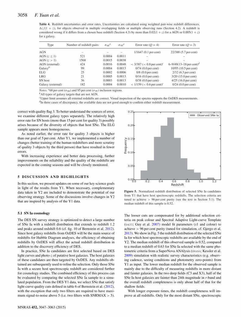
Figure 5. Normalized redshift distribution of selected SNe Ia candidatesfrom Y1 that have host spectroscopic redshifts. The selection criteria aretuned to achieve > 96 per cent purity (see the text in Section 5.1). Themedian redshift of this sample is 0.52.

The looser cuts are compensated for by additional selection cri-teria on peak colour and Spectral Adaptive Light-curve Template(SALT2; Guy et al. 2007) model fit parameters (x1 and colour) toachieve > 96 per cent purity (tuned for simulation, cf. Gjergo et al.2013). We show in Fig. 5 the redshift distribution of the selected SNeIa for which host spectroscopic redshifts are available by the end ofY2. The median redshift of this observed sample is 0.52, comparedto a median redshift of 0.63 for SNe Ia selected with the same pho-tometric criteria from a SuperNova ANAlysis (SNANA; Kessler et al.2009) simulation with realistic survey characteristics (e.g. observ-ing cadence, seeing conditions and photometry zero-points) fromY1 as input. The lower median redshift for the observed sample ismainly due to the difficulty of measuring redshifts in more distantand fainter galaxies. In the two deep fields (C3 and X3), half of theSNe Ia host galaxies are fainter than 24th magnitude in r-band andthe overall redshift completeness is only about half of that for theshallow fields.

With longer exposure times, the redshift completeness will im-prove at all redshifts. Only for the most distant SNe, spectroscopic

MNRAS 452, 3047–3063 (2015)

OzDES Y1 3059

Figure 6. Selected co-added spectra of an SN host target of r-band magnitude 23.7 and redshift 0.732. The significance of the candidate [O II] feature appearsto have increased with exposure time. A quality flag of 3 is assigned so the target will remain in the queue until more data confirm the redshift.

redshifts may remain scarce for host galaxies at typical brightness.This bias against faint host galaxies needs to be considered as it hasbeen shown that stretch and colour-corrected SN Ia peak magni-tude depend on the host galaxy stellar mass (e.g. Kelly et al. 2010;Lampeitl et al. 2010; Sullivan et al. 2010; Childress et al. 2013a).

5.2 Faint SN hosts and spectra stacking

As discussed above, high-redshift efficiency across a wide bright-ness range is critical to maximize the statistics and minimize the biasof a sample of SNe with host galaxy spectroscopic redshifts. Sucha goal is achieved by OzDES’s unique strategy of repeat targeting,dynamic fibre allocation, and stacking. Multiple observations of thesame DES field allows dynamic control of effective exposure timesfor targets of different brightness. The brighter galaxies are des-elected between the observing runs when redshifts are measured;while fainter galaxies remain in the queue. Stacking across manyobserving runs allows OzDES to go deeper than otherwise possiblewith the 3.9 m AAT. Fig. 6 shows an example of stacked spectra,for an SN host target of r-band magnitude 23.7 and redshift 0.732.The growing significance of the emission line, roughly consistentwith square root of exposure time, supports the credibility of thefeature.

5.3 Hostless SNe and super-luminous SNe

We showed in Section 4.1 that redshift efficiency has a differentdependence on target brightness for different types of galaxies. Thelikelihood of measuring an emission line redshift is less sensitiveto apparent broad-band luminosity. A significant fraction of SNe(including most SNe Ia and most core-collapse SNe) are expectedto occur in star-forming regions. For some, strong emission linesmay show up in dispersed AAT spectra even though the continuumis too faint to be detected by DECam imaging in the first fewseasons. A new strategy of targeting hostless SN, by placing a fibreat the position of an SN after the transient has faded, is implemented

after Y1 and has already yielded redshifts that would otherwise beelusive.

This strategy is particularly interesting for validating super-luminous SN (SLSN) candidates. SLSNe are a rare and extremeclass of SN discovered in recent years (Gal-Yam 2012). The originof SLSNe are unclear, but they play a key role in understanding theevolution of massive stars, chemical enrichment and possibly cos-mic re-ionization via their bright UV luminosity. DES will discovermany of these intrinsically bright objects out to redshift about 2.5(Papadopoulos et al. 2015). At high redshifts, the optical (rest-frameUV) spectra of the SLSNe are poorly understood. Redshifts fromhost galaxies are thus crucial to constrain their distances and in-trinsic luminosities. However, SLSNe preferentially occur in dwarfstar-forming galaxies (Lunnan et al. 2014), many of which are toofaint to be detected or to have reliable photo-z estimates from DESmultiband imaging. OzDES provides a cost-effective inspection asthe number of SLSN candidates is large with respect to the timeavailable on 8 to 10 m class telescope, but is small compared to thenumber of AAT fibres. These SLSNe targets will gain high priorityin future AAT observing seasons.

5.4 AGN

We obtained almost 6000 spectra of AGN and AGN candidatesin Y1 (see Section 3.3 for details on the target selection strategyand Fig. 2 for an example spectrum). After the completion of Y1,we identified 989 AGN to monitor. The number of AGN targetsdecreases from 150 per field to 100 per field, but the priority ismaintained at 7 to ensure that the object is observed as frequentlyas possible.

The median redshift of these AGN is 1.63 and the distributionextends to z∼ 4.5 (see Fig. 7). The sample will primarily be analysedusing either the Mg II or C IV emission line, and in some cases bothlines. We will also monitor a substantial number of targets using theH β emission line, which is the most commonly used line in previous

MNRAS 452, 3047–3063 (2015)

3060 F. Yuan et al.

Figure 7. Redshift distribution of the AGN being monitored after the firstyear. Shaded area represents objects that have been observed in five runs ormore by the end of 2014.

reverberation mapping campaigns (e.g. Peterson et al. 2004). Weexpect to accurately recover the radius–luminosity relationship forall three lines (King et al. 2015).

Based on data obtained from 2013 September through the endof 2014, we presently have 5 (6) or more spectroscopic epochs for693 (455) AGN (70 per cent and 46 per cent of the sample). Thesenumbers are close to the expected 7 epochs (in the first two seasons)for 500 AGN in our survey simulation (King et al. 2015). For morethan 10 per cent of the sample, we have acquired spectra in 8 epochs.

5.5 Radio galaxies

By the end of Y1, we had observed 350 targets from the first datarelease of the ATLAS survey (Norris et al. 2006; Middelberg et al.2008), augmenting the earlier work of Mao et al. (2012). Secure red-shifts were obtained for 40 per cent of the targeted sources and themajority currently without redshifts are fainter than mr = 22.5 mag.Sources without a redshift will be re-observed in coming campaignseasons to build up the necessary integration time to determinetheir redshifts and classifications. As we continue to observe thesetargets, we expect to increase our completeness.

With the availability of the ATLAS data release 3 (Franzen et al.in preparation, Banfield et al. in preparation), target selection hasbeen modified slightly after Y1. The additional post-processingprovides higher detection reliability at low radio flux levels leadingto increased sensitivity to low-level star formation.

The redshifts obtained will be used to further the science goalsfor ATLAS including:

(i) to determine the cosmic evolution of both star-forming galax-ies and radio AGN, through the measurement of their redshift-dependent radio luminosity functions. For example, we will be ableto measure luminosity functions for star-forming galaxies to ∼L*(the expected knee of the luminosity function at z = 1).

(ii) to calibrate and develop photometric and statistical redshiftalgorithms for use with the 70 million EMU (Norris et al. 2011)sources (for which spectroscopy is impractical);

(iii) to measure line widths and ratios of emission lines to dis-tinguish star-forming galaxies from AGN, low-ionization nuclearemission-line regions (LINERs), etc., and identify quasars andbroad-line radio galaxies;

(iv) to measure how radio polarization evolves with redshift, asa potential measure of cosmic magnetism.

(v) to explore how morphology and luminosity of radio-loudAGN evolve with redshift, to understand the evolution of the jetsand feedback mechanisms.

5.6 Unusual objects

The large number of spectra taken by OzDES almost guaranteesdiscoveries of rare events or objects. Even in the photometricallyselected samples, outliers are expected to exist. Although an exhaus-tive search for unusual objects is beyond the scope of this work, wehighlight this potential by noting some objects that clearly stand outwhen the spectra were visually inspected in RUNZ. These objects fallin a few broad categories. Although some of these categories arecommon to large transient or spectroscopic surveys, we include allof them to showcase the diversity of the OzDES data set.

(i) Unusual transients: time sensitive observations of live tran-sients are of high priority. To maximize the discovery space, wetarget all transients that satisfy a straightforward magnitude cut.As discussed in Section 3.6, studies of transient spectra have beencomplicated by host galaxy light contamination and data-reductionissues. A more systematic investigation will be carried out whendata reduction is refined.

(ii) Rare stars: at least four WD and M-dwarf binaries are rec-ognized as Galactic objects with both a hot and a cool spectralcomponents. We have also found a WD candidate that is likely arare DQ WD (with carbon bands).

(iii) Broad absorption line AGN: a large number of AGN are ob-served as reverberation mapping targets, radio sources, galaxies, ortransients. More than a dozen of these exhibit extraordinary absorp-tion line systems. Selected objects will be monitored throughoutour survey.

(iv) Serendipitous spectroscopic SN: an SN may be observedunintentionally for two reasons. It happens to occur in a galaxywhere a redshift is desired or it is mis-classified into a different targettype. During the SV season, one of the photo-z targets turned out tobe a Type II SN. The chance for this to happen drops significantlyin subsequent seasons as long-term photometry becomes available.However, the first possibility becomes more likely as more galaxiesare targeted. Approximately one SN occurs every century in a MilkyWay-like galaxy and an SN remains bright for a few weeks to a fewmonths. It is thus expected that every few thousand galaxy spectraat relatively low redshift may contain a visible SN. The concept ofspectroscopic SN search has been successfully tested (Madgwicket al. 2003; Graur & Maoz 2013). However, such a survey methodrequires more than human eyes because the host galaxy light oftendominates and has to be carefully modelled.

(v) Multiple redshifts: if two objects fall in the same fibre, twodistinct sets of spectral features may be observed. Searching fordouble redshifts in galaxy spectra provides a way of finding stronggravitational lens candidates (e.g. Bolton et al. 2004), particularlyfor small Einstein radii and faint background sources that are hard todetect by imaging. Four OzDES targets were noticed to show con-vincing features at two different extragalactic redshifts. Inspectionof the images reveals that two of these are merely chance alignmentbetween background sources and foreground galaxies. The remain-ing two systems are lens candidates, both consisting of a foregroundearly-type galaxy and a background emission line galaxy.

MNRAS 452, 3047–3063 (2015)

OzDES Y1 3061

6 C O N C L U S I O N S

OzDES is an innovative spectroscopic programme that brings to-gether the power of multifibre spectrograph and time series ob-servations. In five years, each DES SN survey field will be tar-geted in about 25 epochs during the DES observing seasons by the2dF/AAOmega spectrograph on the AAT. The 400 fibres are config-ured nightly to target a range of objects with the goal of measuringspectroscopic redshifts of galaxies, monitoring spectral evolutionof AGN or classifying transients. Stacking of multi-epoch spectraallows OzDES to measure redshifts for galaxies that are as faintas mr = 25 mag. Along with efficient redshifting and recycling offibres, we expect to obtain about 2 500 host galaxy redshifts for theDES SN cosmology study. The long-term time series, contempora-neous with DECam imaging, will enable reverberation mapping ofthe largest AGN sample to date. In addition, OzDES is an importantsource of redshifts for various DES photo-z programmes.

In the above sections, we have summarized the OzDES observ-ing strategy, reported results from the first year of operation andevaluated the outcome in light of various science goals. Overall,our strategy has worked well in the first year and produced a largenumber of redshifts with good quality. We are on track to achieveour main science goals. Meanwhile, we have identified a number ofareas for improvements, including better data-reduction proceduresto reduce artefacts and more rigorous cross-check to raise redshiftreliability.

By the time of writing, the second observing season (Y2) hascompleted and already a number of updates have been implemented.Additional data and better understanding of the survey yield has al-lowed us to reassess target selection and de-selection criteria fordifferent target types and science goals. For example, targeting thebrightest objects first maximizes the number of measured redshiftsfor radio galaxies, but such tactics only work when selection bias isnot a major consideration. It is also desirable to abandon an unsuc-cessful target after certain number of exposures, while the maximumintegration time allowed depends on the total number of redshiftsanticipated for this particular target type. Short integration timesallow faster recycling of fibres and more redshifts to be measured.During poor observing conditions, a backup programme is in placeto measure redshifts for bright galaxies, along with high-prioritytargets such as AGN and active transients.

As for all long-term projects, we expect to continue to refineour data quality, actively analyse new data and adapt the observingstrategy in the coming years.

AC K N OW L E D G E M E N T S

Parts of this research were conducted by the Australian ResearchCouncil Centre of Excellence for All-sky Astrophysics (CAAS-TRO), through project number CE110001020. ACR acknowledgesfinancial support provided by the PAPDRJ CAPES/FAPERJ Fel-lowship. This work was supported in part by the US Departmentof Energy contract to SLAC No. DE-AC02-76SF00515. BPS ac-knowledges support from the Australian Research Council LaureateFellowship Grant LF0992131. NS is the recipient of an AustralianResearch Council Future Fellowship. FS acknowledges financialsupport provided by CAPES under contract No. 3171-13-2

The data in this paper were based on observations obtained at theAustralian Astronomical Observatory (AAO programs A/2012B/11and A/2013B/12, and NOAO program NOAO/0278). The authorswould like to thank Marguerite Pierre and the XMM-XXL collabo-

ration for allowing them to use a couple of hours of their time onthe AAT to target the DES C3 field.

The authors would like to thank Charles Baltay and the La SillaQuest Supernova Survey to conduct a concurrent transient searchduring the SV season to help test the targeting strategy. The au-thors are grateful for the extraordinary contributions of their CTIOcolleagues and the DECam Construction, Commissioning and SVteams in achieving the excellent instrument and telescope condi-tions that have made this work possible. The success of this projectalso relies critically on the expertize and dedication of the DES DataManagement group.

Funding for the DES Projects has been provided by the US De-partment of Energy, the US National Science Foundation, the Min-istry of Science and Education of Spain, the Science and Technol-ogy Facilities Council of the United Kingdom, the Higher EducationFunding Council for England, the National Center for Supercomput-ing Applications at the University of Illinois at Urbana-Champaign,the Kavli Institute of Cosmological Physics at the University ofChicago, the Center for Cosmology and Astro-Particle Physics atthe Ohio State University, the Mitchell Institute for FundamentalPhysics and Astronomy at Texas A&M University, Financiadorade Estudos e Projetos, Fundacao Carlos Chagas Filho de Amparoa Pesquisa do Estado do Rio de Janeiro, Conselho Nacional deDesenvolvimento Cientıfico e Tecnologico and the Ministerio daCiencia e Tecnologia, the Deutsche Forschungsgemeinschaft andthe Collaborating Institutions in the Dark Energy Survey.

The DES data management system is supported by the Na-tional Science Foundation under Grant Number AST-1138766.The DES participants from Spanish institutions are partially sup-ported by MINECO under grants AYA2012-39559, ESP2013-48274, FPA2013-47986, and Centro de Excelencia Severo OchoaSEV-2012-0234, some of which include ERDF funds from the Eu-ropean Union.

The Collaborating Institutions are Argonne National Labora-tory, the University of California at Santa Cruz, the University ofCambridge, Centro de Investigaciones Energeticas, Medioambien-tales y Tecnologicas-Madrid, the University of Chicago, UniversityCollege London, the DES-Brazil Consortium, the EidgenossischeTechnische Hochschule (ETH) Zurich, Fermi National Acceler-ator Laboratory, the University of Edinburgh, the University ofIllinois at Urbana-Champaign, the Institut de Ciencies de l’Espai(IEEC/CSIC), the Institut de Fisica d’Altes Energies, LawrenceBerkeley National Laboratory, the Ludwig-Maximilians Universitatand the associated Excellence Cluster Universe, the University ofMichigan, the National Optical Astronomy Observatory, the Uni-versity of Nottingham, The Ohio State University, the Universityof Pennsylvania, the University of Portsmouth, SLAC National Ac-celerator Laboratory, Stanford University, the University of Sussex,and Texas A&M University.

This paper has gone through internal review by the DEScollaboration.

R E F E R E N C E S

Ahn C. P. et al., 2014, ApJS, 211, 17Albrecht A. et al., 2006, preprint (arXiv:astro-ph/0609591)Astier P. et al., 2006, A&A, 447, 31Banerji M. et al., 2015, MNRAS, 446, 2523Bentz M. C. et al., 2013, ApJ, 767, 149Bernstein J. P. et al., 2012, ApJ, 753, 152Blandford R. D., McKee C. F., 1982, ApJ, 255, 419Blondin S., Tonry J. L., 2007, ApJ, 666, 1024

MNRAS 452, 3047–3063 (2015)

3062 F. Yuan et al.

Bolton A. S., Burles S., Schlegel D. J., Eisenstein D. J., Brinkmann J., 2004,AJ, 127, 1860

Brough S., Green A., Bryant J., 2014, AAO Obs., 126, 15Childress M. et al., 2013a, ApJ, 770, 108Childress M. et al., 2013b, Astron. Telegram, 5568, 1Comparat J. et al., 2013, MNRAS, 428, 1498Croom S., Saunders W., Heald R., 2004, AAO Newsl., 106, 12Davies R. I. et al., 2006, ApJ, 646, 754Diehl H. T. et al., 2012, Phys. Procedia, 37, 1332Diehl H. T. et al., 2014, in Peck A. B., Benn C. R., Seaman R. L., eds,

Proc. SPIE Conf. Ser. Vol. 9149, Observatory Operations: Strategies,Processes, and Systems V. SPIE, Bellingham, p. 91490V

Driver S. P. et al., 2011, MNRAS, 413, 971Flaugher B., 2005, Int. J. Mod. Phys. A, 20, 3121Flaugher B. L. et al., 2012, in McLean I. S., Ramsay S. K., Takami, H., eds,

SPIE Conf. Ser., Vol. 8446, Ground-based and Airborne Instrumentationfor Astronomy IV. SPIE, Bellingham, p. 11

Gal-Yam A., 2012, Science, 337, 927Gjergo E., Duggan J., Cunningham J. D., Kuhlmann S., Biswas R., Kovacs

E., Bernstein J. P., Spinka H., 2013, Astropart. Phys., 42, 52Graur O., Maoz D., 2013, MNRAS, 430, 1746Grier C. J. et al., 2013, ApJ, 773, 90Guy J. et al., 2007, A&A, 466, 11Howell D. A. et al., 2005, ApJ, 634, 1190Husemann B., Kamann S., Sandin C., Sanchez S. F., Garcıa-Benito R., Mast

D., 2012, A&A, 545, A137Kaspi S., Brandt W. N., Maoz D., Netzer H., Schneider D. P., Shemmer O.,

2007, ApJ, 659, 997Kelly P. L., Hicken M., Burke D. L., Mandel K. S., Kirshner R. P., 2010,

ApJ, 715, 743Kessler R. et al., 2009, PASP, 121, 1028King A. L., Davis T. M., Denney K. D., Vestergaard M., Watson D., 2014,

MNRAS, 441, 3454King A. L. et al., 2015, preprint (arXiv:1504.03031)Lampeitl H. et al., 2010, ApJ, 722, 566Lewis I. J. et al., 2002, MNRAS, 333, 279Lidman C. et al., 2013, Publ. Astron. Soc. Aust., 30, 1Lunnan R. et al., 2014, ApJ, 787, 138Madgwick D. S., Hewett P. C., Mortlock D. J., Wang L., 2003, ApJ, 599,

L33Mao M. Y. et al., 2012, MNRAS, 426, 3334McMahon R. G., Banerji M., Gonzalez E., Koposov S. E., Bejar V. J., Lodieu

N., Rebolo R., VHS Collaboration, 2013, The Messenger, 154, 35Middelberg E. et al., 2008, AJ, 135, 1276Norris R. P. et al., 2006, AJ, 132, 2409Norris R. P. et al., 2011, Publ. Astron. Soc. Aust., 28, 215Olmstead M. D. et al., 2014, AJ, 147, 75Onken C. A. et al., 2014, ApJ, 791, 37Papadopoulos A. et al., 2015, MNRAS, 449, 1215Peterson B. M., 1993, PASP, 105, 247Peterson B. M. et al., 2004, ApJ, 613, 682Rykoff E. S. et al., 2014, ApJ, 785, 104Sako M. et al., 2011, ApJ, 738, 162Sako M. et al., 2014, preprint (arXiv:1401.3317)Sanchez C. et al., 2014, MNRAS, 445, 1482Sharp R., Birchall M. N., 2010, Publ. Astron. Soc. Aust., 27, 91Sharp R., Parkinson H., 2010, MNRAS, 408, 2495Shen Y. et al., 2015, ApJS, 216, 4Smith G. A. et al., 2004, in Moorwood A. F. M., Iye M., eds, SPIE Conf.

Ser., Vol. 5492, Ground-based Instrumentation for Astronomy. SPIE,Bellingham, p. 410

Sullivan M. et al., 2006, ApJ, 648, 868Sullivan M. et al., 2010, MNRAS, 406, 782Sullivan M. et al., 2011, ApJ, 737, 102van Dokkum P. G., 2001, PASP, 113, 1420Watson D., Denney K. D., Vestergaard M., Davis T. M., 2011, ApJ, 740,

L49Woo J.-H. et al., 2010, ApJ, 716, 269

Wright E. L. et al., 2010, AJ, 140, 1868Yuan F. et al., 2013, Astron. Telegram, 5642, 1Yuan F. et al., 2014, Astron. Telegram, 5757, 1

1Research School of Astronomy and Astrophysics, The Australian NationalUniversity, Canberra, ACT 2611, Australia2ARC Centre of Excellence for All-sky Astrophysics (CAASTRO)3Australian Astronomical Observatory, North Ryde, NSW 2113, Australia4School of Mathematics and Physics, University of Queensland, QLD 4072,Australia5Department of Physics and Astronomy, University College London, GowerStreet, London WC1E 6BT, UK6Kavli Institute for Cosmology, University of Cambridge, Madingley Road,Cambridge CB3 0HA, UK7Institute of Astronomy, University of Cambridge, Madingley Road,Cambridge CB3 0HA, UK8Fermi National Accelerator Laboratory, PO Box 500, Batavia, IL 60510,USA9Observatorio Nacional, Rua Gal. Jose Cristino 77, Rio de Janeiro, RJ-20921-400, Brazil10Laboratorio Interinstitucional de e-Astronomia – LIneA, Rua Gal. JoseCristino 77, Rio de Janeiro, RJ-20921-400, Brazil11Department of Physics and JINA Center for the Evolution of the Elements,University of Notre Dame, 225 Nieuwland Science Hall, Notre Dame, IN46556, USA12INAF–Astrophysics Observatory of Turin, Strada Osservatorio 20, PinoTorinese, I-10025 Torino, Italy13Institut de Ciencies de l’Espai, IEEC-CSIC, Campus UAB, Facultat deCiencies, Torre C5 par-2, E-08193 Bellaterra, Barcelona, Spain14Institute of Cosmology and Gravitation, University of Portsmouth, DennisSciama Building, Burnaby Road, Portsmouth PO1 3FX, UK15Kavli Institute for Particle Astrophysics and Cosmology, PO Box 2450,Stanford University, Stanford, CA 94305, USA16Department of Astronomy, University of Illinois at Urbana-Champaign,1002 W. Green St, Urbana, IL 61801, USA17Department of Physics, University of Illinois at Urbana-Champaign,1110 W. Green St, Urbana, IL 61801, USA18Kavli Institute for Cosmological Physics, University of Chicago, Chicago,IL 60637, USA19Centre for Astrophysics and Supercomputing, Swinburne University ofTechnology, Hawthorn, VIC 3122, Australia20Lawrence Berkeley National Laboratory, 1 Cyclotron Road, Berkeley, CA94720, USA21Dark Cosmology Centre, Niels Bohr Institute, University of Copenhagen,Juliane Maries Vej 30, DK-2100 Copenhagen, Denmark22Argonne National Laboratory, 9700 South Cass Avenue, Lemont, IL60439, USA23Sydney Institute for Astronomy, School of Physics, A28, The University ofSydney, NSW 2006, Australia24Center for Cosmology and Astro-Particle Physics, The Ohio State Uni-versity, Columbus, OH 43210, USA25Department of Astronomy, The Ohio State University, Columbus, OH43210, USA26CSIRO Astronomy and Space Science, Epping, NSW 1710, Australia27CAPES Foundation, Ministry of Education of Brazil, Brasılia, DF 70040-020, Brazil28Astronomy Centre, University of Sussex, Falmer, Brighton BN1 9QH, UK29SLAC National Accelerator Laboratory, Menlo Park, CA 94025, USA30Department of Physics, University of Arizona, 1118 E 4th St, Tucson, AZ85721, USA31Department of Physics and Astronomy, University of Pennsylvania,Philadelphia, PA 19104, USA32International Centre for Radio Astronomy Research, Curtin University,GPO Box U1987, Perth, WA 6845, Australia33School of Physics and Astronomy, University of Southampton, Southamp-ton SO17 1BJ, UK34Department of Physics, Stanford University, 382 Via Pueblo Mall, Stan-ford, CA 94305, USA

MNRAS 452, 3047–3063 (2015)

OzDES Y1 3063

35Cerro Tololo Inter-American Observatory, National Optical AstronomyObservatory, Casilla 603, La Serena, Chile36Institut d’Astrophysique de Paris, Univ. Pierre et Marie Curie and CNRSUMR7095, F-75014 Paris, France37National Center for Supercomputing Applications, 1205 West Clark St,Urbana, IL 61801, USA38George P. and Cynthia Woods Mitchell Institute for Fundamental Physicsand Astronomy, and Department of Physics and Astronomy, Texas A & MUniversity, College Station, TX 77843-4242, USA39Department of Physics, Ludwig-Maximilians-Universitat, Scheinerstr. 1,D-81679 Munchen, Germany40Jet Propulsion Laboratory, California Institute of Technology, 4800 OakGrove Dr., Pasadena, CA 91109, USA41Department of Physics, University of Michigan, Ann Arbor, MI 48109,USA42Max-Planck-Institut fur extraterrestrische Physik, Giessenbachstr.D-85748 Garching, Germany43University Observatory Munich, Scheinerstrasse 1, D-81679 Munich,Germany

44Department of Physics, The Ohio State University, Columbus, OH 43210,USA45ICRA, Centro Brasileiro de Pesquisas Fısicas, Rua Dr. Xavier Sigaud 150,CEP 22290-180, Rio de Janeiro, RJ, Brazil46Department of Astronomy, University of Michigan, Ann Arbor, MI 48109,USA47Institut de Fısica d’Altes Energies, Universitat Autonoma de Barcelona,E-08193 Bellaterra, Barcelona, Spain48Institucio Catalana de Recerca i Estudis Avancats, E-08010 Barcelona,Spain49Brookhaven National Laboratory, Bldg 510, Upton, NY 11973, USA50Centro de Investigaciones Energeticas, Medioambientales y Tecnologicas(CIEMAT), Avda. Complutense 40, E-28040 Madrid, Spain

This paper has been typeset from a TEX/LATEX file prepared by the author.

MNRAS 452, 3047–3063 (2015)