Embed Size (px)
Citation preview
Design of Distributed and Fixed-Structure Controllers
for Cooperative Vehicle Control
Vom Promotionsausschuss der
Technischen Universitat Hamburg-Harburg
zur Erlangung des akademischen Grades
Doktor-Ingenieur (Dr.-Ing.)
genehmigte Dissertation
von
Andrey Popov
aus
Sofia, Bulgarien
2012
Prufungsvorsitzender: Prof. Dr.-Ing. Wolfgang Meyer
Gutachter: Prof. Dr. Herbert Werner
Prof. Dr. Karl-Heinz Zimmermann
Dr. Tamas Keviczky
Tag der mundlichen Prufung: 09.02.2012
To my parents

Cover photo Patrouille Suisse air-show
at 820th Hafengeburtstag, Hamburg 2009
Photo by Andrey Popov

Everything starts somewhere,
although many physicists disagree.
Terry Pratchett

This page is intentionally left blank for pagination.
Contents
Notation xiii
1 Introduction 1
1.1 Current State of Research . . . . . . . . . . . . . . . . . . . . . . . . . . . 2
1.2 Scope and Contribution . . . . . . . . . . . . . . . . . . . . . . . . . . . . 4
1.2.1 Analysis results . . . . . . . . . . . . . . . . . . . . . . . . . . . . . 5
1.2.2 Synthesis results . . . . . . . . . . . . . . . . . . . . . . . . . . . . 5
1.3 Structure of This Thesis . . . . . . . . . . . . . . . . . . . . . . . . . . . . 6
2 Cooperative Vehicle Control 9
2.1 Vehicle Dynamics and Local Controller . . . . . . . . . . . . . . . . . . . . 10
2.2 Information Exchange and Graphs . . . . . . . . . . . . . . . . . . . . . . 12
2.2.1 Graph Theory . . . . . . . . . . . . . . . . . . . . . . . . . . . . . . 13
2.2.2 Describing Information Exchange using the Laplacian Matrix . . . . 15
2.2.3 Time-Varying Topology and Communication Delays . . . . . . . . . 16
2.3 Frameworks for Control of Vehicle Formations . . . . . . . . . . . . . . . . 17
2.3.1 Cooperative Control Framework of Fax and Murray . . . . . . . . . 17
2.3.2 Information-Flow Framework . . . . . . . . . . . . . . . . . . . . . 23
2.3.3 Consensus-Based Control of Vehicle Formations . . . . . . . . . . . 27
2.4 Comparison of the Formation Control Strategies . . . . . . . . . . . . . . . 28
3 Robust Stability Analysis of Multi-Agent Systems 31
3.1 Arbitrary Fixed Topology and Communication Delays . . . . . . . . . . . . 31
3.2 Switching Topology and Time-Varying Communication Delays . . . . . . . 36
3.3 Computational Aspects . . . . . . . . . . . . . . . . . . . . . . . . . . . . . 41
3.4 Areas of Application . . . . . . . . . . . . . . . . . . . . . . . . . . . . . . 44
4 Controller and Filter Synthesis Techniques 49
4.1 Robust Stability Synthesis . . . . . . . . . . . . . . . . . . . . . . . . . . . 50
4.1.1 Information-Flow Filter Synthesis . . . . . . . . . . . . . . . . . . . 50
4.1.2 Controller Synthesis . . . . . . . . . . . . . . . . . . . . . . . . . . 52
4.2 Robust Performance Synthesis . . . . . . . . . . . . . . . . . . . . . . . . . 54
4.2.1 Construction of a Generalized Plant . . . . . . . . . . . . . . . . . . 54
4.2.2 Problem Formulation . . . . . . . . . . . . . . . . . . . . . . . . . . 55
4.2.3 H∞ Performance of a MAS . . . . . . . . . . . . . . . . . . . . . . 57
4.3 Robust Stability – Nominal Performance Synthesis . . . . . . . . . . . . . 59
vii
viii CONTENTS
4.4 Nominal Performance Synthesis . . . . . . . . . . . . . . . . . . . . . . . . 60
4.5 Simultaneous Synthesis of Information Filter and Controller . . . . . . . . 61
5 Fixed-Structure Controller Synthesis 63
5.1 Discrete-time H∞ Synthesis . . . . . . . . . . . . . . . . . . . . . . . . . . 66
5.1.1 Search for a Stabilizing Controller . . . . . . . . . . . . . . . . . . . 67
5.1.2 Minimizing the Closed-Loop H∞ Norm . . . . . . . . . . . . . . . . 68
5.2 Simultaneous Search over Controller and Scalings . . . . . . . . . . . . . . 70
5.2.1 Static Scalings . . . . . . . . . . . . . . . . . . . . . . . . . . . . . . 70
5.2.2 Dynamic Scalings . . . . . . . . . . . . . . . . . . . . . . . . . . . . 71
5.2.3 Replicated Structure Approach . . . . . . . . . . . . . . . . . . . . 74
5.3 Simultaneous Stabilization . . . . . . . . . . . . . . . . . . . . . . . . . . . 76
5.4 Replicated Controller Structure . . . . . . . . . . . . . . . . . . . . . . . . 79
5.4.1 Design Problem . . . . . . . . . . . . . . . . . . . . . . . . . . . . . 79
5.4.2 Gradient Computation . . . . . . . . . . . . . . . . . . . . . . . . . 80
5.4.3 Nominal Performance Design for a MAS . . . . . . . . . . . . . . . 81
6 Simultaneous Synthesis of Consensus and Cooperation Modules 85
6.1 Cooperative Controller Synthesis . . . . . . . . . . . . . . . . . . . . . . . 86
6.2 Separate Synthesis of Information Flow Filter and Local Controller . . . . 87
6.3 Simultaneous Synthesis of Information Flow Filter and Local Controller . . 90
6.3.1 Relative Error Approach . . . . . . . . . . . . . . . . . . . . . . . . 91
6.3.2 Difference Error Approach . . . . . . . . . . . . . . . . . . . . . . . 91
6.3.3 Comparison . . . . . . . . . . . . . . . . . . . . . . . . . . . . . . . 94
6.4 Combined Synthesis of Consensus and Cooperation Modules . . . . . . . . 94
7 Summary, Conclusions and Outlook 101
7.1 Conclusions . . . . . . . . . . . . . . . . . . . . . . . . . . . . . . . . . . . 102
7.2 Outlook . . . . . . . . . . . . . . . . . . . . . . . . . . . . . . . . . . . . . 105
Appendices 109
A Multi-Agent Systems 109
A.1 State-Space Model of a MAS . . . . . . . . . . . . . . . . . . . . . . . . . . 109
A.2 Proof of Theorem 2.3 – Stability of a MAS . . . . . . . . . . . . . . . . . . 111
B Matrix Calculus 113
B.1 Matrix Gradients . . . . . . . . . . . . . . . . . . . . . . . . . . . . . . . . 113
B.2 Chain Rule for Matrix Valued Functions . . . . . . . . . . . . . . . . . . . 113
B.2.1 Real-Valued Functions of Real-Valued Variables . . . . . . . . . . . 113
B.2.2 Real-Valued Functions of Complex-Valued Variables . . . . . . . . . 115
C Gradient Computations 117
C.1 Gradient of an Inverted Matrix . . . . . . . . . . . . . . . . . . . . . . . . 117
C.2 Gradient of the H∞ Norm w.r.t. the System Matrices . . . . . . . . . . . . 118
C.3 Subgradient of the H∞ Norm . . . . . . . . . . . . . . . . . . . . . . . . . 120
CONTENTS ix
C.4 Gradient Computation by Optimization over Controller and Scalings . . . 121
C.4.1 Static Scalings . . . . . . . . . . . . . . . . . . . . . . . . . . . . . . 121
C.4.2 Gradient w.r.t. Dynamic Scalings . . . . . . . . . . . . . . . . . . . 122
D Symbols and Abbreviations 123
Bibliography 131

This page is intentionally left blank for pagination.
Acknowledgment
This thesis is the culmination of my research at the Institute of Control Systems at
Hamburg University of Technology in the period 2006-2010. Pursuing my research was in
the same time a fascinating experience and the most challenging academic task I have had
to face thus far. Many people encouraged and supported me in writing this thesis. Here I
would like to take a moment and acknowledge their help and support.
At first place, I would like to thank my advisor Professor Dr. Herbert Werner for the
guidance, trust and support throughout the years. I am grateful for the stimulating and
open discussions, for the opportunity to learn a lot by tutoring the exercise classes of all
his lectures, for the valuable experiences in analytic thinking and presentation skills. I
want to thank Professor Werner for providing me the right balance between freedom and
guidance for my research.
I would like to thank Prof. Dr. Karl-Heinz Zimmermann and Dr. Tamas Keviczky
for their time and effort in examining this work, and Prof. Dr.-Ing. Wolfgang Meyer for
chairing the examination board.
Working at the Institute of Control Systems was a wonderful experience and I would
like to thank all members of the institute, for being not only good colleagues and friends,
but also for making me feel at home. I would like to thank Birthe von Dewitz for the
good advises and the valuable administrative support. I am grateful to Hossam Abbas,
Martin Durrant, Andreas Kwiatkowski, Sudchai Boonto, Gerwald Lichtenberg, Saulat
Chughtai and Mukhtar Ali for the encouragement during the first months of my study
and the many interesting discussions throughout the years. I want to thank Christian
Schmidt, Andreas Kominek, Mahdi Hashemi, Ahsan Ali, Ulf Pilz and Sven Pfeiffer not
only for the discussions in the area of control systems, but also for the enjoyable trips
and bicycle tours in the area of Hamburg. Special thanks go to Ulf, who has been my
primary discussion partner in the area of cooperative control, a great coauthor and a good
friend. Many thanks to Hossam, Mukhtar and especially Gerwald for sharing an office
with me, and always being there for a scientific discussion or unrelated chat. I shall not
forget to thank all students who chose me as an advisor of their project and thesis works
– for I learned a lot from them. Among those I would like to specially thank Carl Aron
Carls, Hannes Rose and Paul Harmsen, for taking the first steps in the area of cooperative
control together with me.
I would like to thank Robert Babuska, for having me as a guest at the Delft Center for
Systems and Control in 2007, and for the guidance during my visit there. I would also like
to mention the following people, who were my colleagues, friends and discussion partners
at DCSC (in alphabetical order): Jelmer van Ast, Matheu Gerard, Andreas Hegyi, Paolo
Massioni, Ilhan Polat, Justin Rise, Jing Shi and Hong Song.
xi
I am also obliged to my colleagues at Scienlab electronic systems GmbH and my friends
at Ruhr-University Bochum for the valuable support in the months before my exam, and
to Michael Tybel for proofreading the final version of this thesis.
A number of people contributed to this work indirectly by providing their friendship,
support and encouragement. I thank them all for their affection, company and under-
standing, and for being able to distract me when I needed it. I would like to specially
thank Ralf, Franziska, Jenny and Nikola for being good friends and travel companions.
At last, I would like to thank those who never stopped supporting me through the
years. I would like to thank my family, which despite the physical distance was always
there for me when I needed them. I am forever grateful to my parents for backing up
my decision to study abroad, for all the care and support during the years, as well as for
asking “Did you start writing?” already from the second week of my PhD-studies. Finally,
I want to thank my brother Zdravko for being tactful enough to never ask such a question.
Bochum, November 2012
Andrey Popov
xii
Notation
Although a complete list of notation, symbols and abbreviations is provided as an appendix,
it is more of a reference type and it is therefore convenient to introduce some of the notation
in advance. The fields of real numbers, complex numbers, integers and non-negative integers
are denoted by R, C, Z and N0, respectively. Scalar and vector variables are denoted
by lower-case letters, whereas upper-case letters are used for matrices. For a matrix A
its transpose is denoted by AT, the complex conjugate by A∗ and the complex conjugate
transpose by A∗T. The sets of n×m real and complex matrices will be denoted by Rn×m
and Cn×m. Further, Ip will denote a p× p identity matrix; 0 will denote a zero matrix with
appropriate dimensions, and F � 0 (F � 0) will denote that F is a symmetric positive
definite (positive semi-definite) matrix. Element i of a vector a will be denoted by ai,
and the element in row i and column k of a matrix A by Aik. The Kronecker product
will be denoted by ⊗. For a matrix A the notation (the font) A will be used to denote
A = IN ⊗A, where N will be clear from the context, whereas A(p) = A⊗ Ip. The complex
unit will be denoted by j and • will denote a variable clear from the context. The notation
A ∈ A will be used to denote that A belongs to the set A.
For a discrete-time dynamic system P (z) the notation
P (z) =
A B
C D
will be used to denote P (z) = C (zIn − A)−1B+D, where z is a complex variable. For two
dynamic systems P (z) and K(z) of appropriate dimensions, the notation
FL(P (z), K(z)) will denote the lower fractional transformation (LFT) (see, Appendix D
for details).
The notation (the font) u will be used to denote that u is a signal of a multi-agent
system (MAS). Matrices and transfer functions of a MAS will be distinguished by the
notation (the font) A and P(z), with the notable except when the matrix or the transfer
function has the structure IN ⊗A, respectively IN ⊗P (z). In the latter cases, the notation
(the font) A, P(z) will be used to emphasize the structure, where A = IN ⊗ A,
P(z) = IN ⊗ P (z) =
A B
C D
.Finally, theorems and lemmas are numbered within chapters sequentially – i.e., a
theorem following, e.g., Lemma 3.1 will be numbered Theorem 3.2 even if it is the first
theorem in that chapter. Other items, such as definitions and examples are numbered
independently.
xiii

This page is intentionally left blank for pagination.
Chapter 1
Introduction
A flock of birds, a swarm of bees, a colony of termites, a fish school, a herd of buffaloes, as
well as a tribe or a society are all examples where a collection of cooperating individuals
results not in the mere sum of the capabilities of the individuals but brings in additional
benefits. These may be an increased security from predators as in the fish schools and the
buffalo herds, a higher complexity and higher diversity of actions as in bee swarms and
termite colonies, or even energy efficiency as by bird flocks. Technology advances have
made it possible to incorporate new control and navigation capabilities in cars, unmanned
airplanes and vessels, as well as to produce such electro-mechanical systems with actuation
and communication capabilities at ever lower price. Thus, a natural question to ask is
whether such systems could profit from cooperative actions similar to the ones observed in
the nature.
There are many applications envisioned for cooperating robotic vehicles – ranging
from deep-ocean exploration and cartography, extraterrestrial exploration and satellite
clusters for high-resolution deep-space or Earth imaging, through disaster area surveillance,
forest-fire and volcano monitoring, to autonomous cars. The required for these tasks
cooperative autonomous vehicles, such as unmanned aerial vehicles (UAVs), unmanned
underwater vehicles (UUVs), ground vehicles, spacecrafts, etc., have become possible by
recent technology advances in the fields of micro-electronics, nano-technology, batteries,
materials and communications. Controlling such vehicles in a remote fashion, as for example
the remotely controlled reconnaissance UAVs, that have been successfully replacing jet-
fighter planes over the last decade, leads to problems of reliability and performance. The
main reason is that a communication feedback loop between a base station (or an operator)
and the vehicles is required. Such centralized control imposes strong requirements on the
communication network, often requires a large computational power and could result in
a poor performance due to communication delays. Hence, it represents a single point
of failure and leads to a poor reliability. Thus new tools for analyzing and designing
algorithms and strategies for cooperative control of vehicles in a distributed manner are
required.
Because for an effective cooperation a group of vehicles should be able to coordinate
their plans and actions, a means for sharing information between the vehicles is needed
[Ren and Beard, 2008, Axiom 1.1]. This can be done either via dedicated communication
modules and communication channels between the vehicles, or by using on-board sensors
1
2 Chapter 1. Introduction
that allow obtaining information about the neighbors (and the environment). Having
provided this capability, control and communication algorithms for the vehicles should
be designed. These algorithms should guarantee that the vehicles will reach a consensus
on the planned actions, will execute the actions in an efficient manner by simultaneously
satisfying certain performance requirements and will avoid collisions with each other and
with obstacles in the environment. Moreover, the control algorithms need to guarantee
stability and acceptable performance under changing interconnection topology between
the vehicles, since the information exchange depends on the distances between the vehicles,
on obstacles in the environment and can be subject to measurement noise, communication
disturbances, or communication delays.
In addition, often a requirement on the efficiency of the control and communication
algorithms is imposed, due to limited power supply available on autonomous vehicles.
Although better batteries and fuel-cells are continuously developed, their capacity never-
theless limits the operation time of vehicles such as UAVs and UUVs. And whereas one
might not always be able to apply energy saving concepts to the actuation of the vehicles,
energy can be saved by limiting the communication bandwidth, processor frequency and
capabilities, etc., and applying more efficient/simple control algorithms. Moreover, often
the control algorithms are allocated only with a small portion of available processing time,
with the rest allocated to safety algorithms and diagnostics. Those limitations, however,
require rigorous analysis of the vehicles and their interactions, as well as less demanding
communication protocols and control algorithms.
1.1 Current State of Research
As already mentioned, cooperating marine vehicles [Vaccarini and Longhi, 2009],
spacecrafts [Lawson, 2001; Xu et al., 2007; Kong, 1998], aerial vehicles [Ryan et al.,
2004; Frost and Sullivan, 2008] and autonomous cars [Balch and Arkin, 1998; Seetharaman
et al., 2006] are all examples where the cooperative action of multiple vehicles is of interest.
Independent of the physical nature of the vehicles various approaches to the cooperative
control problem have been investigated in the literature. A schematic diagram of a co-
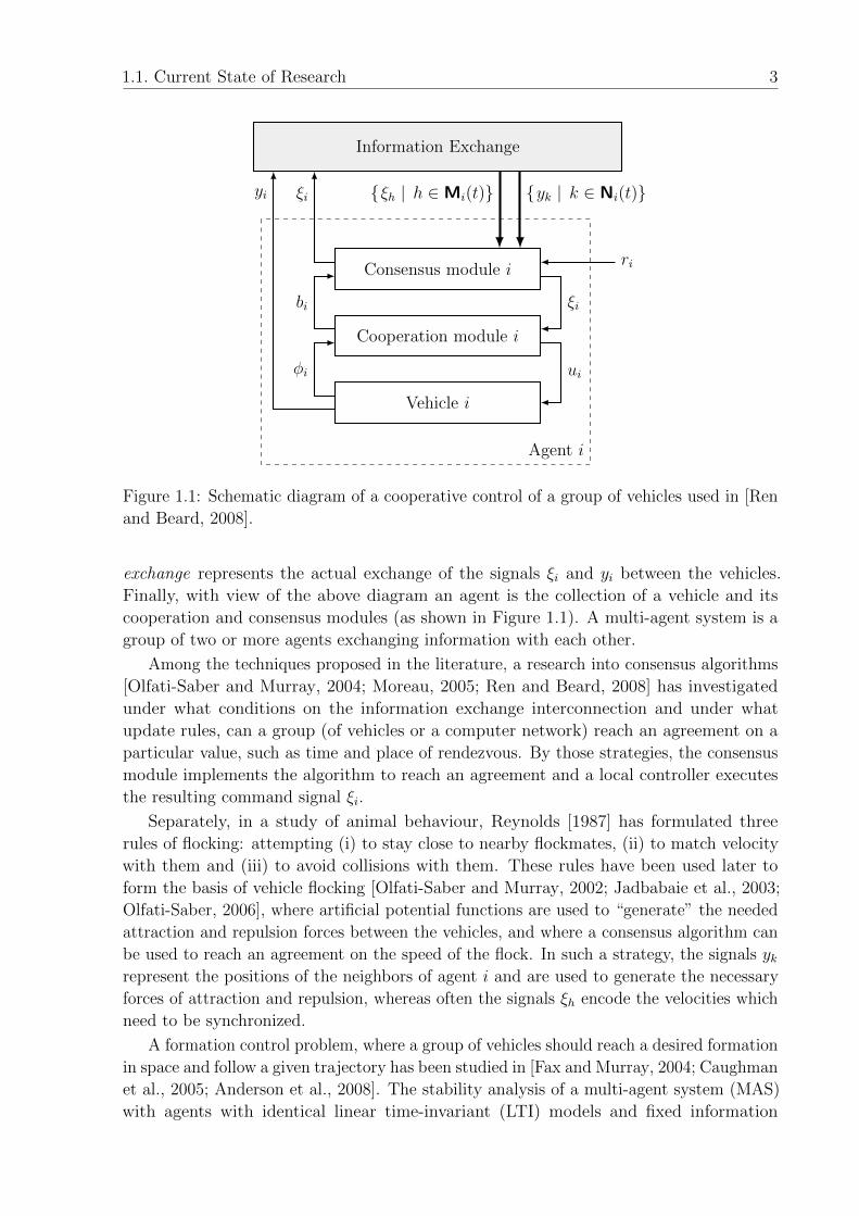
operative control structure presented in [Ren and Beard, 2008], and shown in Figure 1.1,
allows accommodating different approaches by appropriately defining the separate blocks.
In this diagram the block Vehicle i represents the dynamics of vehicle i, which has
ui ∈ Rnu as control input and φi ∈ Rnφ and yi ∈ Rp, p = ny, as outputs. The outputs φirepresent locally available measurements and are used by the block Cooperation module
i to stabilize the vehicle and control its position, orientation and velocity. The signal
ri ∈ Rp represents a command signal that is obtained from an outside source. The signal
ξi ∈ Rq, q = nξ, is called a coordination variable and serves as a commanded/reference
value to the cooperation module. The task of coordinating the actions of the vehicles
in the group is carried out by the consensus modules. Consensus module i receives as
inputs both local feedback bi ∈ Rnb from the cooperation modules, as well as information
about the coordination variables ξh, h ∈Mi and the outputs yk, k ∈ Ni of other vehicles
in its neighborhoods at time t. Here, Mi and Ni are used to denote the corresponding
sets of neighbors and can, in general, be different (i.e., Mi 6= Ni). The block Information
1.1. Current State of Research 3
Information Exchange
Consensus module i
Cooperation module i
Vehicle i
ξi
uiφi
bi
ξiyi {ξh | h ∈Mi(t)} {yk | k ∈ Ni(t)}
ri
Agent i
Figure 1.1: Schematic diagram of a cooperative control of a group of vehicles used in [Ren
and Beard, 2008].
exchange represents the actual exchange of the signals ξi and yi between the vehicles.
Finally, with view of the above diagram an agent is the collection of a vehicle and its
cooperation and consensus modules (as shown in Figure 1.1). A multi-agent system is a
group of two or more agents exchanging information with each other.
Among the techniques proposed in the literature, a research into consensus algorithms
[Olfati-Saber and Murray, 2004; Moreau, 2005; Ren and Beard, 2008] has investigated
under what conditions on the information exchange interconnection and under what
update rules, can a group (of vehicles or a computer network) reach an agreement on a
particular value, such as time and place of rendezvous. By those strategies, the consensus
module implements the algorithm to reach an agreement and a local controller executes
the resulting command signal ξi.
Separately, in a study of animal behaviour, Reynolds [1987] has formulated three
rules of flocking: attempting (i) to stay close to nearby flockmates, (ii) to match velocity
with them and (iii) to avoid collisions with them. These rules have been used later to
form the basis of vehicle flocking [Olfati-Saber and Murray, 2002; Jadbabaie et al., 2003;
Olfati-Saber, 2006], where artificial potential functions are used to “generate” the needed
attraction and repulsion forces between the vehicles, and where a consensus algorithm can
be used to reach an agreement on the speed of the flock. In such a strategy, the signals ykrepresent the positions of the neighbors of agent i and are used to generate the necessary
forces of attraction and repulsion, whereas often the signals ξh encode the velocities which
need to be synchronized.
A formation control problem, where a group of vehicles should reach a desired formation
in space and follow a given trajectory has been studied in [Fax and Murray, 2004; Caughman
et al., 2005; Anderson et al., 2008]. The stability analysis of a multi-agent system (MAS)
with agents with identical linear time-invariant (LTI) models and fixed information
4 Chapter 1. Introduction
exchange topology between the agents has been addressed in [Fax and Murray, 2004].
There, a decomposition-based approach is proposed that reduces the stability analysis of a
MAS with N agents to the simultaneous stability analysis of N transfer functions of the
same order as a single agent. This result has been used later in [Borrelli and Keviczky,
2006; Gu, 2008] for state-feedback controller synthesis and in [Chopra and Spong, 2006;
Massioni and Verhaegen, 2009; Wang and Elia, 2009b] for output feedback controller
synthesis. Additionally, conditions on the information exchange topology for reaching a
consensus and a desired formation are studied in [Moreau, 2005; Chopra and Spong, 2006;
Lee and Spong, 2006; Hirche and Hara, 2008; Wang and Elia, 2009b] to name a few. A
more detailed overview of these and other results will be provided in Section 2.3.
Model predictive control schemes have also been investigated for both formation
control and role assignment purposes [Dunbar and Murray, 2002; Keviczky et al., 2008].
Additionally, strategies for area coverage are explored in [Cortes et al., 2004; Bullo et al.,
2008] and methods for role and task assignment in [Parker, 1998; Klavins and Murray,
2003].
1.2 Scope and Contribution
This thesis investigates the problem of command following of a multi-agent system, where
the command signals ri are obtained either from an outside source (a base station or
an operator) or by a high-level planning and decision modules, and the focus is on the
low level cooperation between the vehicles. Additionally, it is assumed that agents are
described by identical LTI models. The above reviewed analysis and controller synthesis
methods can be used to guarantee the stability and formation acquisition of a multi-agent
system with a known information exchange topology or under certain assumptions on
the interconnection and its evolution in time. However, as the information exchange
between the agents depends on the distances between the vehicles, the obstacles in the
environment and can be subject to communication disturbances and delays, one cannot
generally guarantee that such assumptions will be satisfied. Furthermore, by a MAS with a
large number of agents one might not have a-priori information about the interconnection
topology and the exact communication delays. Moreover, as already discussed, for mobile
agents it is important to develop simple and efficient algorithms that can run on slow and
power-efficient processors.
This thesis work is motivated by decomposition results in [Fax and Murray, 2004] and
results from [Ren and Beard, 2008; Moreau, 2005; Lee and Spong, 2006] and presents tools
for stability analysis and for fixed-structure synthesis of controllers for multi-agent systems
subject to unknown, switching information exchange topology and unknown and possibly
time-varying communication delays. The developed conditions result in a robust analysis
of a single agent with uncertainty and can be efficiently checked. Moreover, as it will be
shown, these conditions are of importance not only for MAS with large number of agents
and uncertain topology, but even for MAS with few agents by which the topology and the
communication delays vary within known sets.
For the purpose of controller synthesis different synthesis problems are defined ranging
from a robust performance synthesis, through a robust stability-nominal performance
1.2. Scope and Contribution 5
synthesis, to a nominal performance synthesis. As it will be shown, the underlying synthesis
problems lead to design problems containing products of decision variables, even when
no restrictions on the structure of the controller are imposed. As such problems cannot
be solved directly, it is shown how gradient-based fixed-structure H∞ controller synthesis
methods can be used for the synthesis. As such optimization-based synthesis techniques
are required, a fixed-structure on the controller can be easily imposed and hence, simple
control laws obtained. Additionally, as the considered scaled H∞ synthesis problem is a
special case of a µ-synthesis, it is shown how the developed tools can be used for µ-synthesis
without iterations over controller and scaling variables.
The contributions of this thesis can be summarized as follows.
1.2.1 Analysis results
• A necessary and sufficient condition for analyzing the stability of a multi-agent system
with arbitrary number of agents, arbitrary but fixed topology and communication
delays. The condition reduces the stability analysis to a structured singular value
analysis of a single agent with uncertainty;
• Sufficient conditions for the stability analyzing of a multi-agent system with arbitrary
number of agents, switching topology and time-varying communication delays. The
condition reduces the stability analysis to either a scaled l1 or a scaled H∞ analysis
of a single agent with uncertainty.
1.2.2 Synthesis results
• A robust performance synthesis, that reduces the problem of controller synthesis
for a MAS with unknown or time-varying topology and communication delays, to a
robust synthesis for a single agent;
• A robust stability–nominal performance synthesis problem, that allows designing a
controller guaranteeing the robust stability of a MAS and the nominal performance
of a single agent;
• A method for synthesis of controllers with replicated structure, which can guar-
antee the nominal performance of a MAS with a fixed and known topology and
communication delays;
• An extension to the above mentioned synthesis methods, that allows simultaneous
synthesis of the consensus and the cooperation module in Figure 1.1;
• A µ-synthesis approach, by which controller and scaling parameters are synthesized
simultaneously, thus avoiding D-K iterations;
• A gradient-based technique for synthesis of discrete-time fixed-structure controllers.
6 Chapter 1. Introduction
1.3 Structure of This Thesis
The thesis is structured as follows. Chapter 2 introduces the dynamic model of the vehicles
and some basic results from graph theory. Then, it shows how three different frameworks
to cooperative vehicle control can be expressed using the block-diagram in Figure 1.1.
The analysis problem is addressed in Chapter 3, where necessary and sufficient conditions
for the robust stability of a MAS are derived. In Chapter 4 these conditions serve as a
basis for defining two alternative design problems of a controller guaranteeing the robust
stability of a MAS under unknown and possibly switching topology and communication
delays. Additionally, the problem of synthesizing a controller that guarantees a nominal
performance for a MAS with a known topology and communication delays is formulated.
In Chapter 5, it is shown how gradient-based tools can be used to attack the non-convex
H∞ synthesis problems, resulting from the robust stability design problems, as well
as from the requirement of a fixed-structure controllers. In Chapter 6 the cooperative
controllers resulting from applying the robust synthesis approach to two of the frameworks
to cooperative control are compared. Additionally, it is shown how the developed synthesis
technique can be used for a simultaneous synthesis of the consensus and the cooperation
modules in Figure 1.1 and what advantages such a synthesis brings. Finally, Chapter 7
summarizes the results and outlines directions for future developments.
The chapters of the thesis are organized in such a way that each of them builds upon its
predecessors. Hence, for a thorough understanding of the matter, it is recommended that
one reads them in the presented order. Nevertheless, readers interested in different aspects
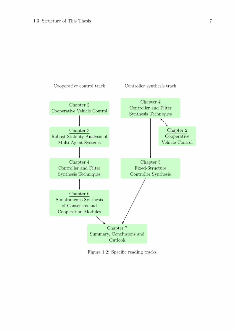
of this work might find it useful to concentrate only on particular chapters. Figure 1.2 shows
two possible paths through this thesis. For readers interested in cooperative vehicle control,
the left part offers an overview of the results of this thesis, without the complexity of the
synthesis algorithms in Chapter 5. On the other hand, for readers primarily interested in
controller synthesis techniques and in particular µ-synthesis and fixed-structure synthesis,
the right path offers the most, with the occasional need to look up some definitions from
Chapter 2.
1.3. Structure of This Thesis 7
Chapter 2
Cooperative Vehicle Control
Chapter 3
Robust Stability Analysis of
Multi-Agent Systems
Chapter 4
Controller and Filter
Synthesis Techniques
Chapter 6
Simultaneous Synthesis
of Consensus and
Cooperation Modules
Chapter 7
Summary, Conclusions and
Outlook
Chapter 4
Controller and Filter
Synthesis Techniques
Chapter 2
Cooperative
Vehicle Control
Chapter 5
Fixed-Structure
Controller Synthesis
Cooperative control track Controller synthesis track
Figure 1.2: Specific reading tracks.

This page is intentionally left blank for pagination.
Chapter 2
Cooperative Vehicle Control
If you don’t know where you are going, any
road will get you there.
Lewis Carroll
In this thesis the problem of cooperative control of a multi-agent system with N
vehicles is considered, in which the vehicles could be mobile robots, UAVs, UUVs, etc.
With regard to the discussion in Chapter 1 and the schematic diagram in Figure 1.1, an
agent and a multi-agent system are defined in this work as follows.
Definition 2.1. An agent is the collection of a vehicle and its cooperation and consensus
modules, as shown in Figure 1.1.
Whereas actual agents will posses additional sensors and actuators that allow them
to interact with the environment, in this work it is assumed that the only interaction
is through the agent outputs yi. For example, if yi are the coordinates of vehicle i in
space, one can use this framework to address problems like formation flight of UAVs, space
interferometry, surveillance of a forest fire, etc., where either the relative to each other or
the absolute positions of the vehicles are of importance.
As the focus of this thesis is on algorithms and tools for stability analysis and controller
synthesis, it will be assumed that the vehicles are point objects and collision free. This is
a valid assumption when the distances between the vehicles are much larger than their
dimensions, when there are no obstacles in the environment and when the vehicles can
move in any direction, or their radius of turning is comparatively small. As those conditions
rarely hold in practice, one will need to consider additional collision avoidance and route
planning techniques, such as artificial potential functions, additional supervisory-control
level, etc. These will be addressed again in the Outlook.
Definition 2.2. A Multi-Agent System (MAS) is a dynamic system comprising of
two or more agents, that can exchange information with each other over communication
channels that may be changing or/and subject to delays.
Note that this definition differs from the typical definitions of MAS in the computer
science and artificial cognition fields (see, e.g., [Wooldridge, 2009]) in the point, that the
9
10 Chapter 2. Cooperative Vehicle Control
emphasis is on the dynamics of the agents and not on their autonomous planning and
decision capabilities, hence addressing a low (cooperative) execution and motion level.
The diagram in Figure 1.1 offers a rather general scheme of cooperative control and
as such accommodates different cooperation problems and strategies. In the following,
the focus will be on the problem of cooperative control of a group of N identical vehicles
with a causal, discrete-time linear time-invariant (LTI) model, controlled by discrete-time
LTI cooperation and consensus modules. Discrete-time modeling is chosen since digital
controllers, digital communication and smart sensors (providing digital rather than analog
readings) are state of the art – and also since – a vehicle model is often obtained by
system identification, resulting in a discrete-time transfer function. Additionally, it will be
assumed that the agents are sequentially indexed from 1 to N , but assigning other indices
or identification numbers to the agents does not change the presented results.
The remainder of this chapter is structured as follows. In Section 2.1, the dynamic
model of the vehicles is presented. Section 2.2 discusses the possible means of information
exchange and shows how graphs can be used as a method of modeling this information
exchange. In Section 2.3, the scheme in Figure 1.1 will be used to provide an unified
view on three MAS control strategies: (i) a cooperative vehicle control framework, (ii) an
information flow-framework proposed in [Fax and Murray, 2004], and (iii) a consensus
based-approach to cooperative control, studied in [Kingston et al., 2005; Ren and Beard,
2008]. Finally, Section 2.4 compares the three strategies and states the open problems
that will be addressed in this work.
2.1 Vehicle Dynamics and Local Controller
In this work a MAS is considered, that consists of N identical vehicles with a causal,
discrete-time LTI model. Let P (z) denote the transfer function of a single vehicle, whose
dynamics are described by the following minimal state-space equations i ∈ [1, N ]xi(t+ 1)
yi(t)
φi(t)
=
AP BP
CPfDPf
CPlDPl
[xi(t)ui(t)
], (2.1)
where t ∈ Z is the discrete time and all signals are zero for t < 0. In the following the
dependence on t will be dropped when clear from the context. Without loss of generality
it will be assumed that the sampling period is one second.
In the above state-space model the subscripts l and f denote, respectively, matrices
associated with local-level and formation-level information channels; xi ∈ Rnx is the system
state vector, ui ∈ Rnu the control input; yi ∈ Rp and φi ∈ Rnφ are measured outputs
(p = ny). Furthermore, process delays are accounted for in the state-space model and the
system matrices are constant and known. Examples 2.1 and 2.2 illustrate these.
2.1. Vehicle Dynamics and Local Controller 11
Example 2.1 (Hovercraft agents). The first example is taken from [Fax and Murray,
2004] and considers the problem of formation control of identical hovercrafts, moving
in an x–y plane. Each hovercraft is equipped with two propellers creating thrust in x
and y direction, and the dynamics in both directions are identical. As a consequence,
the problem can be reduced to a single-dimensional one (control of the y-position). The
one-dimensional dynamics are described by the transfer function
P (z) =yi(z)
ui(z)= 0.05
z + 1
(z − 1)2z−2,
where a sampling time of 0.1 s is used and ui and yi are correspondingly the thrust and
the position (in y-direction) of hovercraft i.
In addition, it is assumed that φi = yi. The local signal φi could be generated, e.g.,
using an Inertial Measurement Unit (IMU) on board of the hovercraft, or by receiving
external positioning information (e.g., using Global Positioning System (GPS)). Each
hovercraft receives information about its neighbours either via communication (e.g.,
radio broadcast) or using on-board sensors such as camera, ultrasonic or laser proximity
sensor. In the latter case agent i measures the distance dik to a neighbour k and using
its own position calculates the coordinates of agent k. A state-space model of an agent,
as in (2.1), is described by the following matrices:
AP =
0 1 0 0
0 0 1 1
0 0 1 2
0 0 0 1
, BP =
0
0
0
0.05
, CPf= CPl
=[1 0 0 0
], DPf
= DPl= 0.
This example has been selected to provide intuitive demonstration and visualization of
many of the concepts and results in this work, and although rather simple encompasses
many features displayed by other MAS.
Example 2.2 (Quadrocopter agents). Consider a fleet of quad-rotor helicopters – quadro-
copters (see, e.g., [Castillo et al., 2005]). Each quadrocopter is propelled by 4 motors,
and obtains information about its position and orientation via an on-board IMU and a
GPS sensor. The local signals φi are the position, the orientation angles and their rates
of variation, i.e., signals needed for the stabilization of a quadrocopter. As on formation
level only the position of the quadrocopters in space is of interest, yi ∈ R3 contains only
the three positions.
12 Chapter 2. Cooperative Vehicle Control
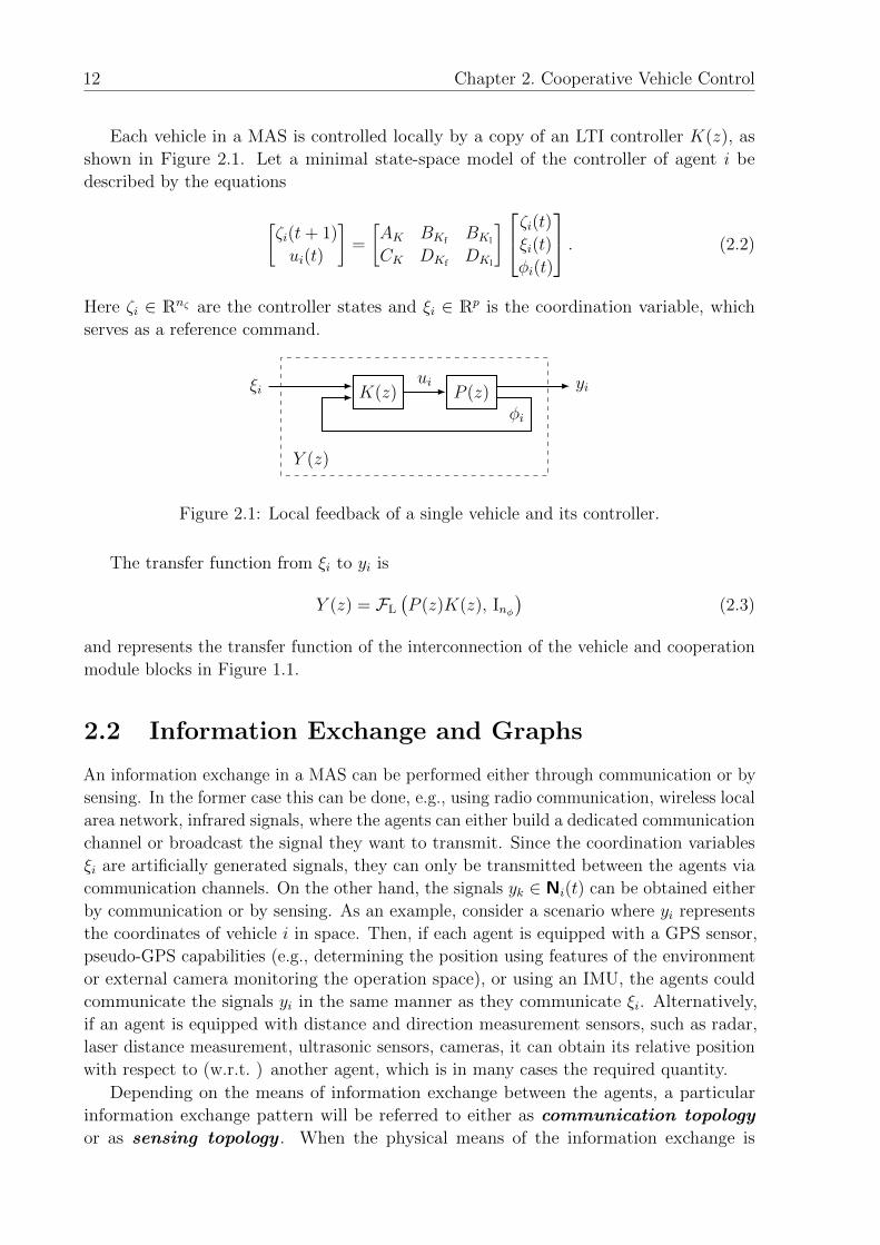
Each vehicle in a MAS is controlled locally by a copy of an LTI controller K(z), as
shown in Figure 2.1. Let a minimal state-space model of the controller of agent i be
described by the equations
[ζi(t+ 1)
ui(t)
]=
[AK BKf
BKl
CK DKfDKl
]ζi(t)ξi(t)
φi(t)
. (2.2)
Here ζi ∈ Rnζ are the controller states and ξi ∈ Rp is the coordination variable, which
serves as a reference command.
K(z) P (z)ξiui yi
φi
Y (z)
Figure 2.1: Local feedback of a single vehicle and its controller.
The transfer function from ξi to yi is
Y (z) = FL
(P (z)K(z), Inφ
)(2.3)
and represents the transfer function of the interconnection of the vehicle and cooperation
module blocks in Figure 1.1.
2.2 Information Exchange and Graphs
An information exchange in a MAS can be performed either through communication or by
sensing. In the former case this can be done, e.g., using radio communication, wireless local
area network, infrared signals, where the agents can either build a dedicated communication
channel or broadcast the signal they want to transmit. Since the coordination variables
ξi are artificially generated signals, they can only be transmitted between the agents via
communication channels. On the other hand, the signals yk ∈ Ni(t) can be obtained either
by communication or by sensing. As an example, consider a scenario where yi represents
the coordinates of vehicle i in space. Then, if each agent is equipped with a GPS sensor,
pseudo-GPS capabilities (e.g., determining the position using features of the environment
or external camera monitoring the operation space), or using an IMU, the agents could
communicate the signals yi in the same manner as they communicate ξi. Alternatively,
if an agent is equipped with distance and direction measurement sensors, such as radar,
laser distance measurement, ultrasonic sensors, cameras, it can obtain its relative position
with respect to (w.r.t. ) another agent, which is in many cases the required quantity.
Depending on the means of information exchange between the agents, a particular
information exchange pattern will be referred to either as communication topology
or as sensing topology . When the physical means of the information exchange is
2.2. Information Exchange and Graphs 13
irrelevant, only the term topology will be used. The topology can be fixed (i.e., time-
invariant) or switching (i.e., time-varying). Variations in the topology might occur due to
communication/sensing range limitations, obstacles, disturbances or when an agent joins
or leaves a MAS. Moreover, the exchanged signals can be subjected to transmission delays
due to limited communication bandwidth, sensor processing times, etc.
Graphs offer a natural way of representing the information exchange topology between
the agents. The following section summarizes some definitions and results on graphs and
graph theory which will be useful in the following (see., e.g., [Ren et al., 2007], [Merris,
1994]).
2.2.1 Graph Theory
A directed graph G (V, E) consists of a non-empty set of vertices V = {1, . . . , N} and
an edge set E ⊆ V × V . Here each vertex represents an agent and each edge corresponds
to an information exchange channel. An edge (k, i) ∈ E indicates that agent i receives
information from agent k. For an edge (k, i) vertex k is called parent and vertex i –
child . Without loss of generality self-edges are not allowed, i.e., (i, i) /∈ E , ∀i ∈ [1, N ].
In schematic diagrams of graphs, a vertex will be marked by a circle and an edge by a
directed arrow from parent to child, i.e., showing the direction of information flow.
An undirected graph is a graph for which the information exchange is always bi-
directional, i.e., (k, i) ∈ E ⇔ (i, k) ∈ E holds. Accordingly, the topology corresponding
to a directed and to an undirected graph will be referred to as a directed topology and
an undirected topology . In this work directed topologies are considered, as they allow
modeling information exchange due to unidirectional wireless communication (broadcast-
ing), camera and proximity sensors, and since the undirected ones can be treated as a
special case.
Finally, an agent that does not receive information from other agents will be referred
to as a leader agent .
The union of n graphs with a common vertex set, G1(V , E1), . . . , Gn(V , En), or shortly
the union of graphs , is a graph G[1,n](V , E[1,n]) = G1 ∪ . . .∪Gn, whose edge set is a union
of the edges E[1,n] = E1 ∪ . . . ∪ En of the collected graphs.
In a directed graph G, a sequence of edges (k, h1), (h1, h2), . . . , (hl, i), starting from
vertex k and ending at vertex i, is called a directed path from k to i. A vertex k is called
globally reachable if there exists a directed path from k to every other vertex. A graph
is said to have a spanning tree if it has at least one globally reachable vertex. If every
vertex is globally reachable, then the graph is strongly connected (or simply connected
for undirected graphs).
The set of neighbours Ni of agent i is the set of agents from which agent i receives
information:
Ni := {k | (k, i) ∈ E} .
The cardinality of the set, i.e., the number of agents from which agent i receives information,
will be denoted by |Ni|.Adjacency, Laplacian and incidence matrices can be used to describe a graph mathe-
matically. In this work only the former two are used. The adjacency matrix J ∈ RN×N
14 Chapter 2. Cooperative Vehicle Control
of a graph G (V, E) with N vertices is defined as
Jik :=
{1 if (k, i) ∈ E ,0 if (k, i) /∈ E .
(2.4)
Let dini (respectively dout
i ) denote the in-degree (out-degree) of vertex i, i.e., the number
of vertices that have vertex i as child (as parent):
dini =
N∑k=1
Jik, douti =
N∑k=1
Jki.
Since the elements of J are either zero or positive, dini is non-negative, with din
i = 0 only
when agent i is a leader.
The results presented in this work will hold also for weighted graphs, i.e., graphs by
which each edge is assigned with a positive weight (in eq. (2.4)), as long as each agent
normalizes the incoming signals by dini . In fact, for the (unweighted) graphs considered in
this work dini = |Ni|, ∀i holds. Furthermore, a graph is balanced if din
i = douti , ∀i ∈ [1, N ].
All undirected graphs are balanced and satisfy J = J T.
The (normalized) Laplacian matrix L of a graph is defined as follows.
Lik :=
1 if i = k and |Ni| 6= 0,
− 1|Ni| if k ∈ Ni,
0 otherwise.
(2.5)
Let Θ := {χ | χ ∈ C, |χ| < 1} denote the open unit disk , O := {χ | χ ∈ C, |χ| = 1}the unit circle and Θ := Θ ∪O the closed unit disk . Let P denote the Perron disk
P := 1 + Θ. Then the following is true.
Theorem 2.1. Let λi ∈ spec(L), ∀i ∈ [1, N ], denote the eigenvalues of the Laplacian L.
Then λi ∈ P, ∀i ∈ [1, N ].
The proof follows by applying Gersgkorin disk’s theorem to L (see, e.g., [Meyer, 2000,
p. 498] or [Horn and Johnson, 1985, Theorem 6.1.1]).
Moreover, as the sum of the elements of each row of L is zero, λ1 = 0 is always an
eigenvalue of L. Hence, L is not invertible.
For undirected graphs the eigenvalues of L are real (cf. [Ren et al., 2007]) λi ∈ [0, 2],
∀i ∈ [1, N ]. The second smallest eigenvalue, λ2 is referred to as the algebraic connectivity
of the graph (cf. [Ren et al., 2007; Tuna, 2008]).
As the sensing/communication topology can be always reconstructed from the Laplacian,
in the following L will be used to denote the topology.
2.2. Information Exchange and Graphs 15
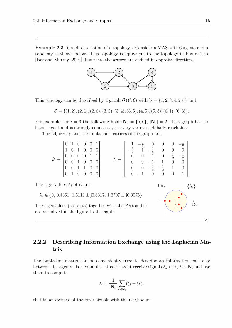
Example 2.3 (Graph description of a topology). Consider a MAS with 6 agents and a
topology as shown below. This topology is equivalent to the topology in Figure 2 in
[Fax and Murray, 2004], but there the arrows are defined in opposite direction.
1 2 4
6 3 5
This topology can be described by a graph G (V, E) with V = {1, 2, 3, 4, 5, 6} and
E = {(1, 2), (2, 1), (2, 6), (3, 2), (3, 4), (3, 5), (4, 5), (5, 3), (6, 1), (6, 3)}.
For example, for i = 3 the following hold: N3 = {5, 6}, |N3| = 2. This graph has no
leader agent and is strongly connected, as every vertex is globally reachable.
The adjacency and the Laplacian matrices of the graph are:
J =
0 1 0 0 0 1
1 0 1 0 0 0
0 0 0 0 1 1
0 0 1 0 0 0
0 0 1 1 0 0
0 1 0 0 0 0
, L =
1 −12
0 0 0 −12
−12
1 −12
0 0 0
0 0 1 0 −12−1
2
0 0 −1 1 0 0
0 0 −12−1
21 0
0 −1 0 0 0 1
.
The eigenvalues λi of L are
λi ∈ {0, 0.4361, 1.5113± j0.6317, 1.2707± j0.3075}.
The eigenvalues (red dots) together with the Perron disk
are visualized in the figure to the right.
Re
Im
1
{λi}
2.2.2 Describing Information Exchange using the Laplacian Ma-
trix
The Laplacian matrix can be conveniently used to describe an information exchange
between the agents. For example, let each agent receive signals ξk ∈ R, k ∈ Ni and use
them to compute
`i =1
|Ni|∑k∈Ni
(ξi − ξk),
that is, an average of the error signals with the neighbours.
16 Chapter 2. Cooperative Vehicle Control
Define ` =[`1 . . . `N
]Tand ξ =
[ξ1 . . . ξN
]T. Then, the above computation can
be written in a compact form for the whole MAS as
` = Lξ.
2.2.3 Time-Varying Topology and Communication Delays
The above definitions hold for delay-free time-invariant graphs. However, in reality
the information exchange between the vehicles in a formation will change depending
on the distance between the vehicles, on communication/sensing range limitations, on
obstacles in the environment, when new agents join or when agents are damaged or leave
the communication range. Furthermore, the information obtained from other agents
will be usually delayed due to sensing/communication delays, bandwidth limitations,
communication disturbances or sensing noise. In the following the term communication
delay will be used, regardless whether the delay is with communication or sensing origin.
Hence, one can define a switching graph G(t) = G(V(t), E(t)), which for every time
instance t is a fixed graph Gt = Gt(Vt, Et).Assume now that the information exchange from agent k to agent i is associated with
a communication delay τik(t) ∈ N0, ∀i, k ∈ [1, N ], i 6= k. Note that process delays (if
present) are assumed to be accounted for in the system model P (z) in (2.1). Furthermore,
it is assumed that the internal signals in the agents are not delayed, that is τii = 0,
∀i ∈ [1, N ]. As an example, in the case of time-varying communication delays, the agents
will be computing locally the following signal
`i(t) =1
|Ni|∑k∈Ni
(ξi(t)− ξk(t− τik(t))).
Assume that communication topology and time delays are time-invariant and define a
frequency dependent Laplacian as follows:
Lik(z) =
1, if i = k and |Ni| 6= 0
− 1|Ni|z
−τik , if k ∈ Ni
0, otherwise.
(2.6)
Then, one can write the above equation for the whole MAS as `(z) = L(z)ξ(z). In addition,
one can show the following result which will be used later on.
Lemma 2.2. When evaluated along the unit disk z = ejω, ω ∈ [−π, π] the eigenvalues
λi(ω) of the frequency dependent normalized Laplacian L(ejω) satisfy λi(ω) ∈ P.
Proof. By Gersgkorin’s disk theorem [Meyer, 2000] for a fixed ω the eigenvalues λi(ω) of
L(ejω) satisfy
|λi(ω)− Lii(ejω)| ≤N∑k=1
|Lik(ejω)|.
Using that Lii(ejω) = 1 and that for each τik ∈ N0 and ω ∈ [−π, π]
|Lik(ejω)| =∣∣∣∣− 1
|Ni|e−jωτik
∣∣∣∣ =1
|Ni||e−jωτik | = 1
|Ni|,
leads to |λi(ω)− 1| ≤ 1 ⇔ λi(ω) ∈ P, ∀i ∈ [1, N ]. �
2.3. Frameworks for Control of Vehicle Formations 17
2.3 Frameworks for Control of Vehicle Formations
With the help of the above definitions and the block-diagram in Figure 1.1, the three frame-
works mentioned earlier, (i) a cooperative vehicle control framework, (ii) an information
flow-framework proposed in [Fax and Murray, 2004], and (iii) a consensus based-approach
to cooperative control, studied in [Kingston et al., 2005; Ren and Beard, 2008], to control
of vehicle formations can be viewed in a consistent manner.
In the following, H(z) will be used to denote the transfer function from an averaged
error signal inside an agent to the outputs of the same agent that are communicated to or
sensed by other agents. This will be illustrated shortly.
2.3.1 Cooperative Control Framework of Fax and Murray
A cooperative vehicle approach, introduced by Fax and Murray [2004], assumes that the
agents exchange only output signals yi (i.e., signals ξi are not communicated) and each
agent computes the coordination variables ξi as a formation control error signal:
ξi = ei =1
|Ni|∑k∈Ni
eik, (2.7)
where
eik = rik − (yi − yk), (2.8)
and rik ∈ Rp is a desired distance between the outputs of the agents i and k. In other
words, the formation error ei of agent i is the average of the differences between the desired
distances rik (between the outputs of agent i and the outputs of the agents k ∈ Ni from
which it received information) and the differences of the outputs of the agents (yi − yk).This is illustrated in Figure 2.2 for agent i, where k1, k2, . . . , k|Ni| ∈ Ni are the indices of
the agents from which agent i receives information. Note that this corresponds to the
agent in Figure 1.1 with Y (z) being the interconnection of the vehicle and cooperation
blocks (as shown in Figure 2.1) and a consensus block performing the calculation in (2.7).
As discussed earlier, for a fleet of mobile robots and under the condition that yicontains the coordinates of agent i in the operating space, the information exchange can
be performed in the following manner:
• Each agent is aware of its own position and communicates it to the others. Using
the received positions of its neighbours, agent i computes ei;
• Agent i measures the relative distance to each of its neighbours, i.e., yk − yi and
compares it to rik in order to compute eik.
In this framework H(z) = Y (z) holds, as the averaged error used in agent i is the
coordination value ξi, which serves as command to Y (z), and the transmitted/sensed
outputs are the outputs yi of Y (z).
Note that by the above definition of the formation error, each agent is required to know
a complete set of commanded distances rik with respect to each of the agents from which

18 Chapter 2. Cooperative Vehicle Control
rik1
yk1
rik2
yk2
......
1
|Ni|Y (z) yi
rik|Ni|
yk|Ni|
eik1
eik2
eik|Ni|
ei = ξi
−
−
−
Agent i
Figure 2.2: Computation of the formation error of agent i and the agent’s boundary.
it can receive information. In fact, since the topology might change during the operation
of the MAS, the agents are required to know a complete set of commanded distances with
respect to all other agents. Further, in order for the agents to be able to attain these
distances, the references should be consistent, i.e., for a consistent reference signals
rik = −rki and rij +rjk = rik hold for ∀i, j, k ∈ [1, N ]. However, for the purpose of analysis
and controller synthesis, it suffices to consider the signals rik as a reference signals for the
MAS.
Closed-Loop System
Using the definition of the normalized Laplacian in (2.5), one can construct the overall
formation error e =[eT1 . . . eTN
]Tand the closed-loop of the MAS as follows. Let
L(p) = L ⊗ Ip, y =[yT1 . . . yTN
]Tand let r denote a reference signal, that directly
defines a commanded value for the outputs of the agents. Then, using (2.7) and the
definition of L one can write
e =L(p)(r − y) = L(p)e = r − L(p)y, (2.9)
where e = r − y is an absolute position error, and r denote a reference for the relative
position of the agents in the formation. Note that, since L is not invertible, to the same
relative references r correspond infinitely many absolute references r. The closed-loop
interconnection of the whole MAS, with the absolute reference r as input is shown in
Figure 2.3. If, instead, one wants to use the relative reference r, one needs to insert it
after the block L(p). Note that in Figure 2.3 the only interaction between the agents is via
2.3. Frameworks for Control of Vehicle Formations 19
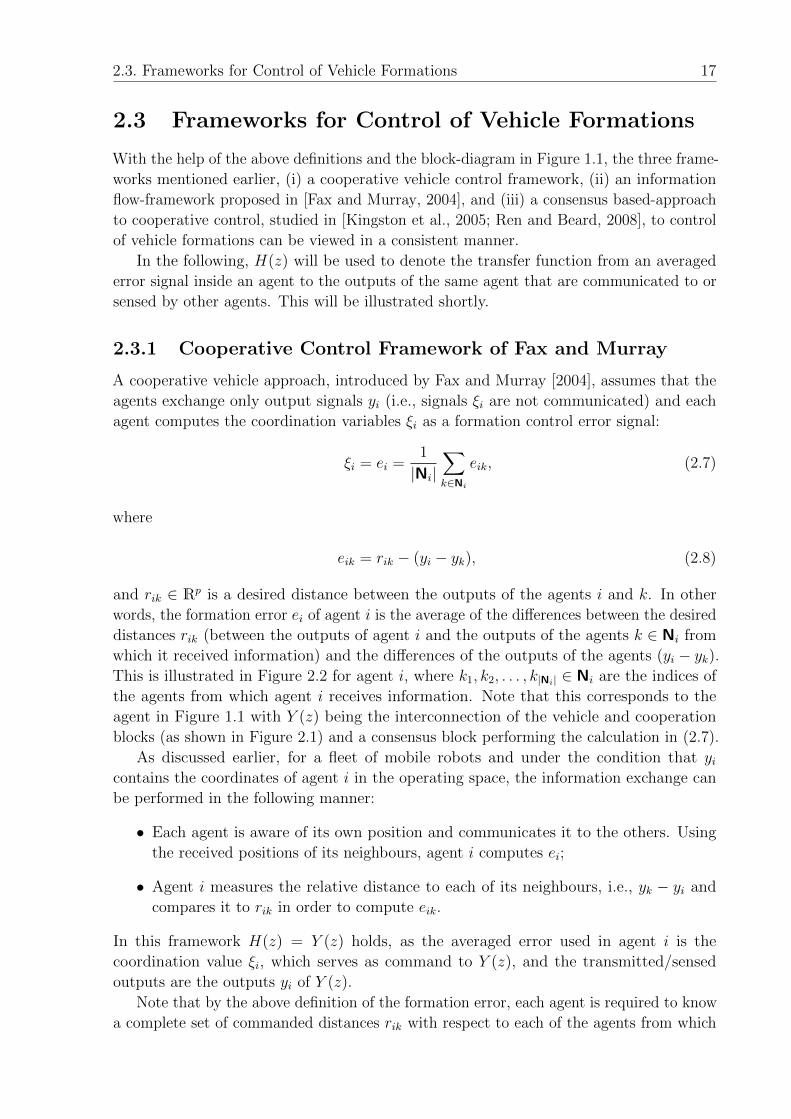
the communication/sensing topology L(p). Furthermore, note that it is necessary to define
L(p) = L ⊗ Ip in order to account for the dimension of yi and compare the corresponding
output signals.
H(z)
r L(p)...
y
H(z)
e e
e1
eN
y1
yN−
S(z)
Figure 2.3: Closed-loop representation of a multi-agent system.
For the dynamic transfer function H(z) =
AH BH
CH DH
define H(z) as the Kronecker
product IN ⊗H(z), i.e.:
H(z) = IN ⊗H(z) =
IN ⊗ AH IN ⊗BH
IN ⊗ CH IN ⊗DH
=
AH BH
CH DH
. (2.10)
It is important to note that for a general matrix X ∈ RN×N
X ⊗H(z) 6=
X ⊗ AH X ⊗BH
X ⊗ CH X ⊗DH
.Then, the closed-loop MAS, i.e., the transfer function from reference input r ∈ RpN to
the outputs of the agents y ∈ RpN , can be written in a compact form as
S(z) =(
IpN + H(z)L(p)
)−1
H(z)L(p). (2.11)
The complete closed-loop state-space model of the MAS is provided in Appendix A.1.
Stability Analysis for a Fixed Topology
For a fixed topology the stability of a MAS is defined as follows.
Definition 2.3 (MAS stability). A MAS is (strictly) stable if all eigenvalues of the
system matrix of S(z) lie strictly inside the unit disk Θ. A MAS is neutrally stable if
one eigenvalue is at 1 + j0, but all others lie strictly inside Θ.
In order to determine the stability of the closed-loop MAS, one needs to check the
eigenvalues of the system matrix of S(z). To avoid eigenvalue computation for MAS with
large number of agents and states, a decomposition-based approach proposed by [Fax and
Murray, 2004] can be applied.
20 Chapter 2. Cooperative Vehicle Control
Theorem 2.3 (MAS stability). Consider a multi-agent system with N agents, a fixed
topology without communication delays described by L, a vehicle dynamics P (z) as in
(2.1), a controller K(z) as in (2.2) and let H(z) = FL(P (z)K(z), Inφ) (i.e., as in (2.3)).
The following statements are equivalent.
(a) The closed-loop MAS S(z) (see Figure 2.3) is stable.
(b) The transfer function FL (−λiIp, H(z)) is stable for ∀λi ∈ spec(L),
(c) The interconnection FL
(Pλi(z),
[−Ip 0
0 Inφ
]K(z)
), is stable for ∀λi ∈ spec(L),
where Pλi(z) are transfer functions with a state-space realizationx(t+ 1)
yi(t)
φi(t)
=
AP BP
λiCPfλiDPf
CPlDPl
[xi(t)ui(t)
]. (2.12)
The above theorem states that the stability of a multi-agent system is equivalent to the
simultaneous stability of N transfer functions, having the same dynamics as a single agent,
but scaled by a (possibly complex) scalar λi. This result is derived via a state, input and
output transformation of the MAS S(z) and therefore, the states xi, inputs ui and outputs
yi, φi of the transfer functions Pλi(z) do not correspond to those of the agents P (z) in
(2.1).
The theorem above differs from Theorem 3 in [Fax and Murray, 2004] in that feed-
through terms (DPland DPf
) are allowed. The proof is based on performing a state,
input and output transformation of the closed-loop MAS using a matrix Q, such that
Q−1LQ is a diagonal or triangular matrix (e.g., Q being a matrix of eigenvectors of L or
a matrix performing a Schur decomposition on L). For completeness the proof is provided
in Appendix A.2.
This decomposition result is used in [Fax and Murray, 2004] to develop the following
Nyquist-diagram-based stability test for SISO systems H(z).
Theorem 2.4 (SISO stability test). A MAS with a fixed topology without communication
delays and described by L is stable if and only if the net encirclements of the points − 1λi
by the Nyquist diagram of H(z) is zero, ∀i ∈ [1, N ].
An extension to MIMO systems, based on the spectral radius stability condition
[Skogestad and Postlethwaite, 2005, Theorem 4.9], has also been proposed, but provides
only a sufficient condition for stability:
Theorem 2.5 (MIMO stability test). For a MAS with a fixed topology without commu-
nication delays and described by L let β ≥ |1− λi| ∀i ∈ [1, N ]. Then a controller K(z)
stabilizes the MAS if
ρ(T (ejω)
)<
1
β, ∀ω ∈ [0, π],
where ρ(T (ejω)
)denotes the spectral radius of T (ejω) = (I +H(ejω))−1H(ejω).
2.3. Frameworks for Control of Vehicle Formations 21
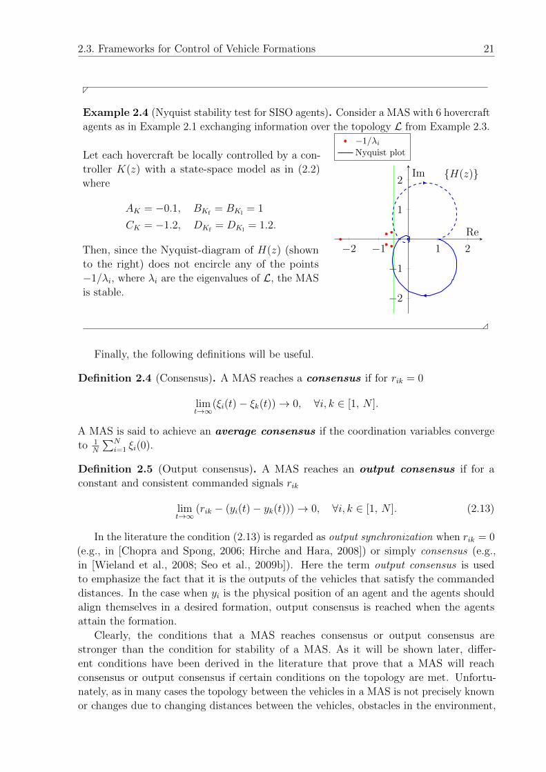
Example 2.4 (Nyquist stability test for SISO agents). Consider a MAS with 6 hovercraft
agents as in Example 2.1 exchanging information over the topology L from Example 2.3.
Let each hovercraft be locally controlled by a con-
troller K(z) with a state-space model as in (2.2)
where
AK = −0.1, BKf= BKl
= 1
CK = −1.2, DKf= DKl
= 1.2.
Then, since the Nyquist-diagram of H(z) (shown
to the right) does not encircle any of the points
−1/λi, where λi are the eigenvalues of L, the MAS
is stable.
−2 −1 1 2
−2
−1
1
2{H(z)}
Re
Im
−1/λiNyquist plot
Finally, the following definitions will be useful.
Definition 2.4 (Consensus). A MAS reaches a consensus if for rik = 0
limt→∞
(ξi(t)− ξk(t))→ 0, ∀i, k ∈ [1, N ].
A MAS is said to achieve an average consensus if the coordination variables converge
to 1N
∑Ni=1 ξi(0).
Definition 2.5 (Output consensus). A MAS reaches an output consensus if for a
constant and consistent commanded signals rik
limt→∞
(rik − (yi(t)− yk(t)))→ 0, ∀i, k ∈ [1, N ]. (2.13)
In the literature the condition (2.13) is regarded as output synchronization when rik = 0
(e.g., in [Chopra and Spong, 2006; Hirche and Hara, 2008]) or simply consensus (e.g.,
in [Wieland et al., 2008; Seo et al., 2009b]). Here the term output consensus is used
to emphasize the fact that it is the outputs of the vehicles that satisfy the commanded
distances. In the case when yi is the physical position of an agent and the agents should
align themselves in a desired formation, output consensus is reached when the agents
attain the formation.
Clearly, the conditions that a MAS reaches consensus or output consensus are
stronger than the condition for stability of a MAS. As it will be shown later, differ-
ent conditions have been derived in the literature that prove that a MAS will reach
consensus or output consensus if certain conditions on the topology are met. Unfortu-
nately, as in many cases the topology between the vehicles in a MAS is not precisely known
or changes due to changing distances between the vehicles, obstacles in the environment,
22 Chapter 2. Cooperative Vehicle Control
communication disturbances and failure one cannot a-priori guarantee that the desired
conditions on the topology will be met. Nevertheless, as it will be shown later on, one
can design the controller of the agents in such a way that a robust stability of a MAS is
guaranteed (w.r.t. to not “precise knowledge” or changes of the topology and the commu-
nication delays), such that when the conditions on the topology are satisfied consensus or
output consensus will be achieved.
Analysis and Synthesis Results
The above theorems offer only stability analysis and cannot be directly used for synthesis of
controllers for formation control. However, the results serve as a basis for several synthesis
and analysis methods proposed in the literature, a short overview over some of which
follows.
A state-feedback synthesis method that reduces the problem from synthesis for a MAS
with N agents to a LQR synthesis for a reduced size MAS with 1 + maxi dini agents, where
dini is the in-degree (see page 14), has been proposed in [Borrelli and Keviczky, 2006].
In [Tuna, 2008] the synthesis problem is reduced to an LQR synthesis for a single agent
depending on the algebraic connectivity λ2. It is then shown that the resulting controller
will in fact guarantee the stability also under every topology with Re {λ2} greater than the
one for which the design has been performed. A state-feedback approach, based on game
theory, has been considered in [Gu, 2008]. Additionally, in [Scardovi and Sepulchre, 2009]
a stability condition for MAS with switching topology (without communication delay) has
been proposed, which requires that the agents exchange estimated system states and the
controller states.
The results of [Fax and Murray, 2004] have been also used for output-feedback control
of passive systems in [Chopra and Spong, 2006], where a sufficient condition for stability
under undirected, connected and fixed topology, but subject to time-varying information
delays is presented. Further, a sufficient condition for stability and output consensus of
dissipative systems is proposed in [Hirche and Hara, 2008].
An H∞ condition for achieving output consensus of general (heterogeneous) LTI SISO
agents under a topology with a globally reachable vertex is presented in [Lee and Spong,
2006]. For identical agents and connected, undirected topology an alternative proof of
Theorem 2.3 and a condition for output consensus is provided for SISO and MIMO agents
in [Seo et al., 2009a,b]. For MIMO agents, a strongly connected topology, and under the
condition that dini = din
k does not hold for every ik pair, an H∞ synthesis approach is
proposed in [Wang and Elia, 2009b] that reduces to a synthesis for a single agent. It is
further shown that if the synthesis is performed for a topology with dmax = maxi dini , then
the controller will guarantee the output consensus also for strongly connected topologies
with smaller maximal in-degree. A further approach, addressing also the problem of
collision avoidance via the use of a dedicated sensing topology and artificial potential
function, is studied in [Chopra et al., 2008]. There it is shown that for second order
(possibly non-linear) systems stabilizable with a static feedback gain, and for a fixed
and balanced topology with fixed communication delays, the agents will reach output
consensus, while avoiding collisions with each other at the same time.
2.3. Frameworks for Control of Vehicle Formations 23
A decomposition-based approach to H2 and H∞ controller synthesis for a MAS with a
fixed topology L has been proposed in [Massioni and Verhaegen, 2009]. The synthesis is
reduced to a set of Linear Matrix Inequalities (LMIs) corresponding to synthesis conditions
for the transfer function Pλi , where λi are the vertices of a convex hull containing all
eigenvalues of L. This is particularly advantageous in the case of undirected topology,
as then the synthesis is reduced to the LMIs for only two vertices, as λ ∈[0 2
]and a
so-obtained controller will guarantee the stability under every undirected topology without
communication delays (this will be discussed in Section 3.4).
However, with the above techniques one can design controller for a MAS with fixed
and known topology or for a certain set of topologies, but none of them can provide
controller guaranteeing the stability of the multi-agent system under an arbitrary fixed
or switching topology. This is an important issue, since in [Fax and Murray, 2004] it
is shown by a simple example that a controller providing good performance for a given
topology might not even stabilize the MAS, when an additional information channel is
added to the topology. As shown later in Section 3.4, this issue becomes acute already by
MAS with moderate number of agents, as the number of “meaningful” topologies increases
exponentially and verifying the stability under each of them becomes an untractable
problem. Furthermore, among the above techniques only the approaches in [Chopra and
Spong, 2006] and [Chopra et al., 2008] can handle communication delays, but the first one
is restricted to passive systems and the latter one is applicable only to fixed topology and
fixed communication delays. Additionally, all of the design methods result in a controller
of an order at least equal to the order of the plant. This, as discussed in the introduction,
is often too high for implementation on a vehicle due to the limited on-board capabilities.
2.3.2 Information-Flow Framework
As an attempt to allow design of MAS that will remain stabile under an arbitrary topology,
in [Fax and Murray, 2004] a modification to the framework, introduced in Section 2.3.1, is
proposed. In addition to the sensing/communication topology L, the agents are assumed
to exchange additional information over a communication topology Lcom. That is, in
view of Figure 1.1 the agents exchange both output information as well as additional,
coordination-type, information.
In order to simplify the following diagrams and equations, assume that the local
feedback over φi is closed and accounted for in P (z), and let C(z) denote the local
controller of the vehicles. Then the information flow filter approach, proposed in [Fax
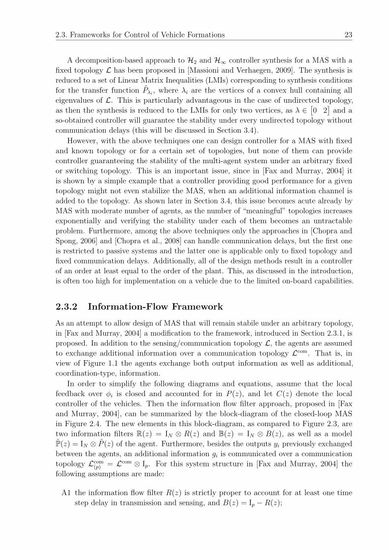
and Murray, 2004], can be summarized by the block-diagram of the closed-loop MAS
in Figure 2.4. The new elements in this block-diagram, as compared to Figure 2.3, are
two information filters R(z) = IN ⊗ R(z) and B(z) = IN ⊗ B(z), as well as a model
P(z) = IN ⊗ P (z) of the agent. Furthermore, besides the outputs yi previously exchanged
between the agents, an additional information gi is communicated over a communication
topology Lcom(p) = Lcom ⊗ Ip. For this system structure in [Fax and Murray, 2004] the
following assumptions are made:
A1 the information flow filter R(z) is strictly proper to account for at least one time
step delay in transmission and sensing, and B(z) = Ip −R(z);
24 Chapter 2. Cooperative Vehicle Control
IpN − Lcom(p)
r L(p) R(z) C(z) P(z) y
B(z) P(z)
e g u− −
Figure 2.4: Information flow framework.
A2 the information exchange topology Lcom coincides with the sensing/communication
topology L, i.e., Lcom ≡ L;
A3 the agent model P (z) is identical to the plant, i.e., P (z) = P (z).
The following theorem is proved in [Fax and Murray, 2004] and establishes the existence
of a separation principle. Let F(z) = IN ⊗ F (z), where F (z) = (Ip −R(z))−1R(z).
Theorem 2.6 (Theorem 6.6 in [Fax and Murray, 2004]). Under assumptions A1–A3 a
MAS is stable if and only if C(z) stabilizes P (z) and the negative feedback interconnection
of F(z) with Lcom(p) is stable.
A proof shown in [Pilz et al., 2011] and alternative to the one given in [Fax and Murray,
2004] is provided here for completeness.
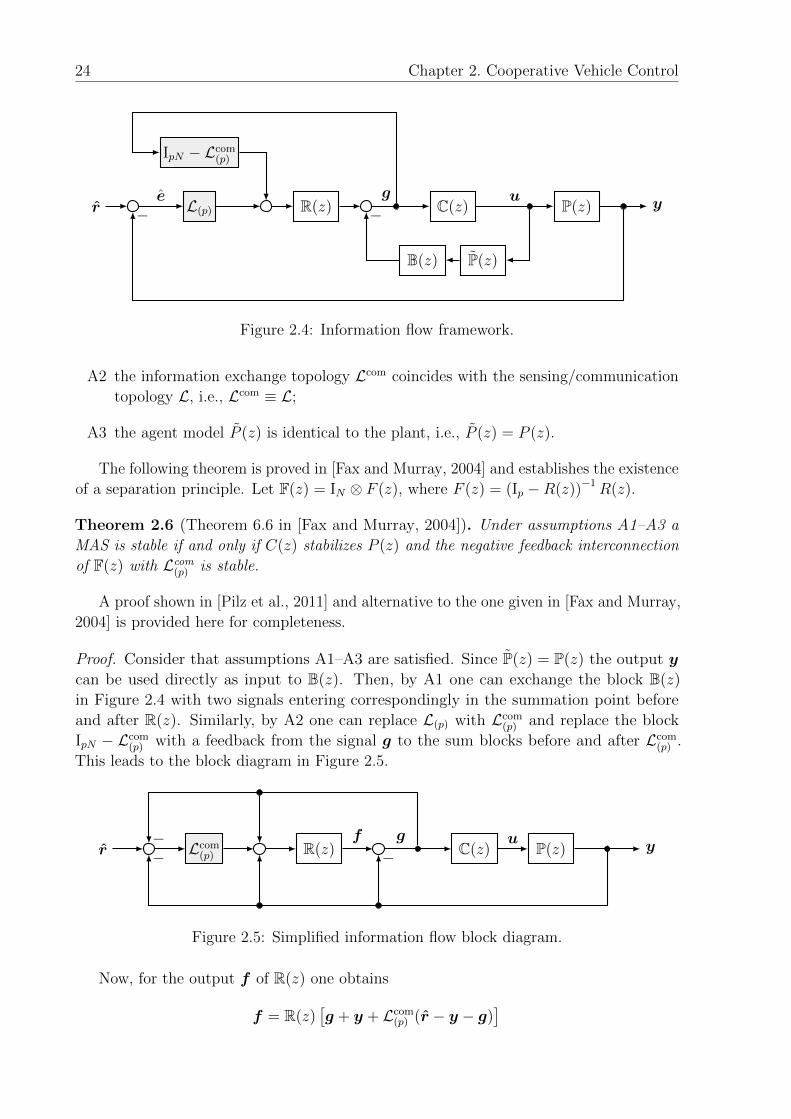
Proof. Consider that assumptions A1–A3 are satisfied. Since P(z) = P(z) the output y
can be used directly as input to B(z). Then, by A1 one can exchange the block B(z)
in Figure 2.4 with two signals entering correspondingly in the summation point before
and after R(z). Similarly, by A2 one can replace L(p) with Lcom(p) and replace the block
IpN − Lcom(p) with a feedback from the signal g to the sum blocks before and after Lcom
(p) .
This leads to the block diagram in Figure 2.5.
r Lcom(p) R(z) C(z) P(z) y
f g u−−
−
Figure 2.5: Simplified information flow block diagram.
Now, for the output f of R(z) one obtains
f = R(z)[g + y + Lcom
(p) (r − y − g)]
2.3. Frameworks for Control of Vehicle Formations 25
which, after substituting g = f − y and using that F (z) = (Ip −R(z))−1R(z) leads to
f = R(z)[f + Lcom
(p) (r − f)]
= R(z)f + R(z)Lcom(p) (r − f)
= (IpN − R(z))−1 R(z)Lcom(p) (r − f)
= F(z)Lcom(p) (r − f)
=(IpN + F(z)Lcom
(p)
)−1 F(z)Lcom(p) r.
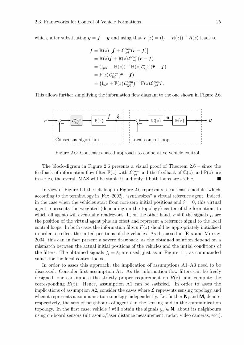
This allows further simplifying the information flow diagram to the one shown in Figure 2.6.
r Lcom(p) F(z) C(z) P(z) y
f = ξ u
Consensus algorithm Local control loop
− −
Figure 2.6: Consensus-based approach to cooperative vehicle control.
The block-digram in Figure 2.6 presents a visual proof of Theorem 2.6 – since the
feedback of information flow filter F(z) with Lcom(p) and the feedback of C(z) and P(z) are
in series, the overall MAS will be stable if and only if both loops are stable. �
In view of Figure 1.1 the left loop in Figure 2.6 represents a consensus module, which,
according to the terminology in [Fax, 2002], “synthesizes” a virtual reference agent. Indeed,
in the case when the vehicles start from non-zero initial positions and r = 0, this virtual
agent represents the weighted (depending on the topology) center of the formation, to
which all agents will eventually rendezvous. If, on the other hand, r 6= 0 the signals fi are
the position of the virtual agent plus an offset and represent a reference signal to the local
control loops. In both cases the information filters F (z) should be appropriately initialized
in order to reflect the initial positions of the vehicles. As discussed in [Fax and Murray,
2004] this can in fact present a severe drawback, as the obtained solution depend on a
mismatch between the actual initial positions of the vehicles and the initial conditions of
the filters. The obtained signals fi = ξi are used, just as in Figure 1.1, as commanded
values for the local control loops.
In order to asses this approach, the implication of assumptions A1–A3 need to be
discussed. Consider first assumption A1. As the information flow filters can be freely
designed, one can impose the strictly proper requirement on R(z), and compute the
corresponding B(z). Hence, assumption A1 can be satisfied. In order to asses the
implications of assumption A2, consider the cases where L represents sensing topology and
when it represents a communication topology independently. Let further Ni and Mi denote,
respectively, the sets of neighbours of agent i in the sensing and in the communication
topology. In the first case, vehicle i will obtain the signals yk ∈ Ni about its neighbours
using on-board sensors (ultrasonic/laser distance measurement, radar, video cameras, etc.).
26 Chapter 2. Cooperative Vehicle Control
One method to ensure that the two topologies coincide is to require that the agents reject
sensing or information signals from the neighbours from which they don’t receive both
types of signals, i.e., use only Ni ∩Mi as neighbours. However, this might lead to a very
sparse or a disconnected topology. Alternatively, the agents could employ a multi-hop
communication algorithm, i.e., vehicles relaying the signals received from their neighbours,
but this could be difficult to implement due to limited communication bandwidth and could,
moreover, result in an excessive communication overhead. Besides, the realization problems
with any of the above approaches, a further problem faced in this scenario is the different
communication delays of y and g signals at the receiving agent. Furthermore, as in this
case a model P (z) of the agent will be needed and since modeling errors and disturbances
are always present, the practical applicability of the strategy becomes questionable.
In the latter case, when the agents in the MAS communicate with each other over
a topology Lcom, it is natural to utilize the same communication links to exchange the
signals gi. Hence Ni ≡Mi and A2 holds. Furthermore, as each agent should be able to
measure/obtain its own output yi in order to communicate it to the others, there is no
need for the model P (z). Hence, assumption A3 holds. Therefore, in the case when the
vehicles in a formation do not use sensor data, but only communicate with each other, the
block-diagram in Figure 2.6 reveals two further aspects of the information flow framework
(shown only recently in [Pilz et al., 2011]):
• The only signals exchanged between the agents are in fact the signals ξi = fi;
• As the outputs yi of the agents are not communicated, input and output disturbances
acting on one vehicle will not be detected by the other vehicles.
Since in this latter case, the interconnection of the agents in a MAS is exactly the one
depicted in Figure 2.6 this strategy turns out to be equivalent to a consensus-based
approach to cooperative vehicle control, studied independently in [Kingston et al., 2005;
Ren and Beard, 2008] and discussed in the next section. Note that in this case the transfer
function of agent i from formation error
`i =1
|Ni|∑k∈Ni
(rik − (ξi − ξk))
to communicated outputs ξi is H(z) = F (z).
Finally, despite its features and its close relation to the cooperative control strategy,
introduced in the very same paper (see Section 2.3.1), the information flow approach
has received little attention. In fact, with exception to the sources of origin [Fax, 2002;
Fax and Murray, 2004] where a heuristically-tuned filter F (z), guaranteeing the stability
under arbitrary topology, is proposed and a short note in [Ren and Beard, 2008], no other
references to the information-flow approach appear to be present in the cooperative control
literature.
2.3. Frameworks for Control of Vehicle Formations 27
2.3.3 Consensus-Based Control of Vehicle Formations
In order for a multi-agent system to fulfill tasks, such as formation acquisition, trajectory
tracking, etc., the agents should share a consistent view of the objective and operation
information. This has motivated research into rules used by the agents and conditions on
the agent interaction that guarantee that the agents will converge to such a consistent
view. Such protocols are called consensus algorithms and represent a set of rules that
each agent should follow, and constitute the consensus module in the schematic diagram
in Figure 1.1.
Clearly, the consensus-based approach is applicable only in cases when the agents can
communicate with each other, i.e., the information exchange is over a communication
topology Lcom. Additionally, in the consensus literature it is typically assumed that the
agents are stable and the cooperation signal ξi serves as a command to the local loop of
agent i. As a consequence, the focus is left on the consensus loop in Figure 2.6 alone.
One of the most often used consensus protocols is assuming a single integrator dynamics
[Olfati-Saber et al., 2007], where each agent updates its coordination state ξi ∈ R using
the rule
ξi(t+ 1) = ξi(t) + ε1
|Mi|∑h∈Mi
(ξh(t)− ξi(t)),
where Mi is the set of agents, from which agent i receives the coordination signals and
0 < ε < 1 is an update step-size. Then, by defining ξ =[ξ1 . . . ξN
]Tand letting ξ(0)
denote the initial state of the MAS, the above algorithm can be written in a compact form
as
ξ(t+ 1) = (IN − εLcom)ξ(t) = ξ(t)− ε`(t).This is equivalent to the feedback loop of F(z) and Lcom in Figure 2.6 with the choice
F (z) = εz−1
.
Single and double integral agent dynamics have been also used in continuous-time
consensus protocols. For example, the system ξ(t) = −Lcomξ(t) represents a first order
continuous-time protocol, t ∈ R. This can be fit in a continuous-time equivalent of the
information consensus loop in Figure 2.6 with F (s) = 1s, where s is the continuous-time
Laplace variable.
Consensus protocols with integral dynamics are well investigated in the literature –
see [Ren et al., 2007; Olfati-Saber et al., 2007] for an overview. Olfati-Saber and Murray
[2004] show that strong connectivity is a sufficient condition for achieving consensus for
general graphs and a necessary and sufficient for balanced graphs (by fixed communication
topology and no communication delays). Additionally, they prove that consensus can
be reached under a switching communication topology G(t) if the topology is strongly
connected for every t ∈ N0, and under a fixed undirected communication topology with
identical delays τik = τ , ∀i, k ∈ [1, N ] if the topology is connected.
Their results are improved upon in the case of fixed communication topology and
no communication delays in [Ren and Beard, 2003], where it is shown that a sufficient
condition for consensus is the existence of a globally reachable node. In the case of
switching communication topology without communication delays, Jadbabaie et al. [2003]
show that for undirected graphs, and Ren and Beard [2004, Theorem 3.5] for the general
case, that a necessary and sufficient condition for consensus is that there exists an infinite
28 Chapter 2. Cooperative Vehicle Control
sequence of bounded intervals [th, th + lh], with th+1 = th + lh + 1, h = 1, 2, . . . , such that
G[th,th+lh] = Gth ∪ . . . ∪ Gth+lh has a globally reachable node.
Consensus protocols with higher order dynamics have been also studied. In
[Moreau, 2005] it is shown that, under an assumption that the update of the state
of each agent belongs to the convex hull of the states of its neighbours (convexity), a MAS
achieves consensus under switching communication topology if and only if there exists an
l ≥ 0 such that G[t,tl] = Gt ∪ . . . ∪ Gt+l has a globally reachable node ∀t ∈ N0. A sufficient
condition for consensus of a MAS with continuous time SISO consensus algorithm and a
globally reachable agent is obtained in [Wieland et al., 2008]. It is further shown, that
the condition is also a necessary one for single and double integrators. The effects of
bounded self delays (i.e., 0 < τii < τ) and symmetric communication delays τik = τki ≤ τ ,
∀i, k ∈ [1, N ] on the consensus of continuous-time SISO filters F (s) is studied in [Munz
et al., 2008, 2009a,b]. In [Munz et al., 2009a], under the assumption that all states of
F (s) are communicated, a consensus analysis condition that is necessary and sufficient for
protocols with self delays and only sufficient for protocols without self delays is derived.
Moreover, as the consensus loop in Figure 2.6 has the same structure (with H(z) = F (z))
as the feedback loop in Figure 2.3, one can apply results on output consensus from [Lee
and Spong, 2006; Seo et al., 2009a,b; Wang and Elia, 2009b] to the consensus achievement
problem.
2.4 Comparison of the Formation Control Strategies
Three strategies to cooperative vehicle control have been reviewed: (i) a cooperative
control approach, (ii) an information flow approach and (iii) a consensus-based approach.
Out of the three the information flow approach appears to be the most versatile, as it
contains the remaining two as special cases. Indeed, in Figure 2.4 the choice R(z) = Ip,
B(z) = 0 and Lcom = IN , is equivalent to no additional information exchange and hence
the cooperative strategy (Section 2.3.1). On the other hand, by satisfying assumptions
A1–A3 and under the condition that L is a communication (and not sensing) topology,
the information flow approach reduces to the consensus-based strategy (Section 2.3.3).
From the discussion above and the structure of the frameworks the following advantages
of the consensus-based strategy over the cooperative control strategy should be obvious.
• The local controller C(z) can be designed independently and tuned for good reference
tracking and disturbance rejection. In fact, as controller Ci(z) is required to stabilize
vehicle Pi(z), ∀i ∈ [1, N ] the approach is also applicable to MAS with heterogeneous
agents.
• A consensus filter F (z) can be chosen with faster dynamics than the vehicle dynamics,
thus allowing faster convergence of the coordination variables ξi. Then, in the limiting
case when the convergence occurs in one time-step, the local loop will perceive ξi as
a step reference command which could be followed in a nominal manner.
However, as pointed out in [Ren and Beard, 2008], this method is mainly applicable to
control of “algorithmically coupled” systems, i.e., systems by which the agents do not
physically influence each other. Examples of the opposite, that is multi-agent systems
2.4. Comparison of the Formation Control Strategies 29
with physical coupling, are vehicle platoons (e.g., automated cars driving on a highway)
and tight UAV formations (e.g., UAVs flying in the wake of their neighbours to reduce
drag), where it is imperative that disturbance signals are propagated to or detected by the
neighbours. Additionally, the decoupling of the vehicle dynamics from the consensus blocks
could cause problems due to non-exact initial conditions for the coordination variables.
Hence, in those cases the outputs signals yi need to be exchanged as well, and a structure
like the one described in Section 2.3.1 might be preferred.
Independent of the choice of cooperative control framework, four problems remain
open.
P1 Robust stability analysis of a MAS subjected to arbitrary topology or to switching
topology and time-varying communication delays;
P2 Synthesis of a controller or/and filter guaranteeing the robust stability of a MAS under
arbitrary fixed or switching topology and imposing certain performance requirements;
P3 Simultaneous synthesis of a local controller and a consensus algorithm (e.g., informa-
tion filter);
P4 Synthesis of low-complexity control laws, i.e., controllers and filters of restricted
order or fixed-structure, that still satisfy the above requirements.
Regarding problem P1, in the existing literature on consensus algorithms the conditions for
achieving consensus or output consensus are studied, but this is done either for simple first
and second order dynamics of the information flow filter or under restrictive assumptions
on the topology.
At the same time, in the case of first order consensus algorithms, or by using a
heuristically tuned information filter, as the one proposed in [Fax and Murray, 2004], one
can guarantee the stability under arbitrary topology, but this approach does not exploit
the characteristics of the local loop. That is, in view of the diagram in Figure 2.6, the
consensus algorithm serves as a pre-filter for the local control loop and as such needs to be
correspondingly tuned. Even better, in order to fully explore the advantages of exchanging
both yi and ξi as information, the controller and the filter should be simultaneously tuned.
Additionally, the advantages of both a simultaneous synthesis of information flow filter
and local controller, as well as synthesis of a controller combining both the consensus
module and the cooperation module in Figure 1.1 should be explored.
Finally, problems P2 and P4 refer to the fact that none of the controller synthesis
methods in Section 2.3.1 can be directly applied to the design of a controller guaranteeing
the stability of a MAS with LTI agents under switching topology and communication
delays, or to design simple (fixed-structure or fixed-order) controllers even for a MAS with
a fixed and known topology.
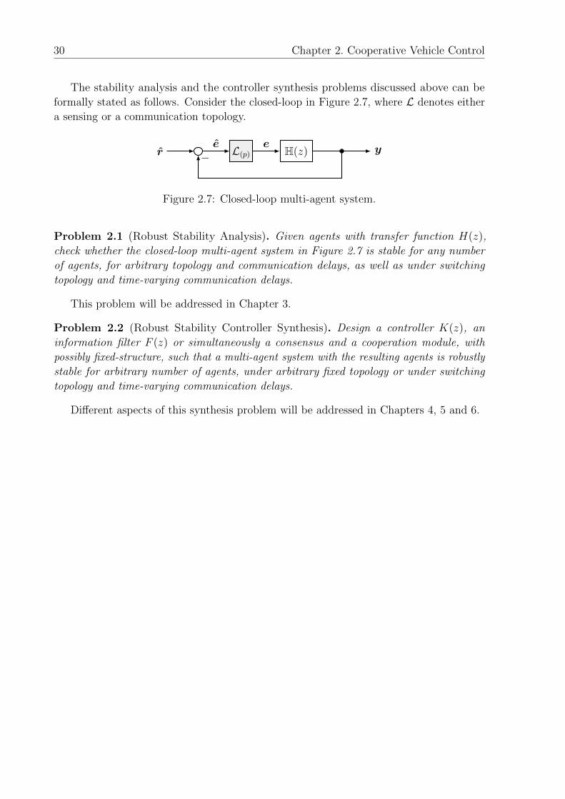
30 Chapter 2. Cooperative Vehicle Control
The stability analysis and the controller synthesis problems discussed above can be
formally stated as follows. Consider the closed-loop in Figure 2.7, where L denotes either
a sensing or a communication topology.
r L(p) H(z) ye e−
Figure 2.7: Closed-loop multi-agent system.
Problem 2.1 (Robust Stability Analysis). Given agents with transfer function H(z),
check whether the closed-loop multi-agent system in Figure 2.7 is stable for any number
of agents, for arbitrary topology and communication delays, as well as under switching
topology and time-varying communication delays.
This problem will be addressed in Chapter 3.
Problem 2.2 (Robust Stability Controller Synthesis). Design a controller K(z), an
information filter F (z) or simultaneously a consensus and a cooperation module, with
possibly fixed-structure, such that a multi-agent system with the resulting agents is robustly
stable for arbitrary number of agents, under arbitrary fixed topology or under switching
topology and time-varying communication delays.
Different aspects of this synthesis problem will be addressed in Chapters 4, 5 and 6.
Chapter 3
Robust Stability Analysis of
Multi-Agent Systems
Don’t Panic.
The Hitchhiker’s Guide to the Galaxy
Douglas Adams
In this chapter, the robust stability analysis problem introduced at the end of Chapter 2
will be studied. For that purpose the stability of the feedback loop in Figure 2.7 will
be analyzed under arbitrary and switching topologies L. Additionally, since the transfer
function H(z) can represent the feedback of a vehicle model and controller by the coop-
erative control approach in Figure 2.3 (i.e., H(z) = FL (P (z)K(z), Im)), as well as the
dynamics of the information filter in the consensus-based approach as in Figure 2.1 (i.e.,
H(z) = F (z)), the presented analysis techniques can be applied to both frameworks.
In what follows, first the stability analysis for a MAS with unknown but fixed number
of agents, topology and communication delays will be considered. Then the analysis will
be extended to a switching topology and time-varying communication delays. The former
problem is of interest, when vehicles with a given controller are used for different tasks,
but during the execution of a particular task the topology remains constant.
3.1 Arbitrary Fixed Topology and Communication
Delays
According to Theorem 2.3, a MAS with a topology L without communication delays will
be stable if and only if the interconnection FL (−λIp, H(z)) is stable for all eigenvalues
λi ∈ spec(L). Correspondingly, a MAS will be stable under an arbitrary topology without
communication delays, if and only if the interconnection of λi and H(z) is stable for all
eigenvalues of every conceivable topology L. However, directly analyzing the stability
using this approach is computationally unattractive as the number of possible topologies,
and hence the number of distinct eigenvalues, increases exponentially with the number of
agents in a MAS. Furthermore, the decomposition approach of [Fax and Murray, 2004]
and correspondingly Theorem 2.3 cannot be directly used for analyzing the stability of a
31
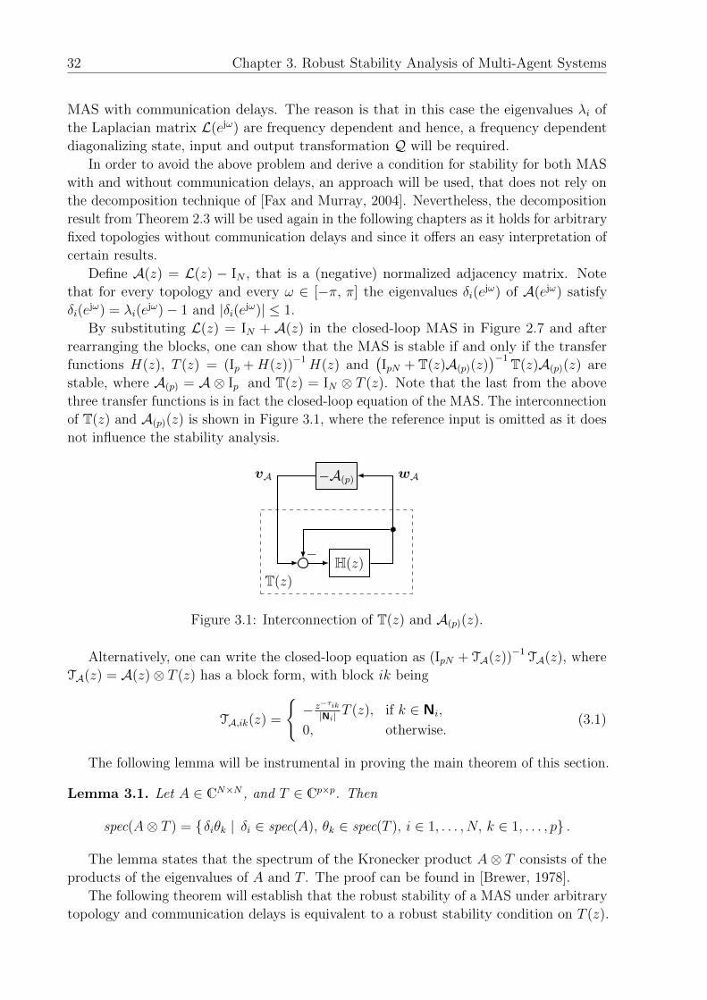
32 Chapter 3. Robust Stability Analysis of Multi-Agent Systems
MAS with communication delays. The reason is that in this case the eigenvalues λi of
the Laplacian matrix L(ejω) are frequency dependent and hence, a frequency dependent
diagonalizing state, input and output transformation Q will be required.
In order to avoid the above problem and derive a condition for stability for both MAS
with and without communication delays, an approach will be used, that does not rely on
the decomposition technique of [Fax and Murray, 2004]. Nevertheless, the decomposition
result from Theorem 2.3 will be used again in the following chapters as it holds for arbitrary
fixed topologies without communication delays and since it offers an easy interpretation of
certain results.
Define A(z) = L(z) − IN , that is a (negative) normalized adjacency matrix. Note
that for every topology and every ω ∈ [−π, π] the eigenvalues δi(ejω) of A(ejω) satisfy
δi(ejω) = λi(e
jω)− 1 and |δi(ejω)| ≤ 1.
By substituting L(z) = IN + A(z) in the closed-loop MAS in Figure 2.7 and after
rearranging the blocks, one can show that the MAS is stable if and only if the transfer
functions H(z), T (z) = (Ip +H(z))−1H(z) and(IpN + T(z)A(p)(z)
)−1 T(z)A(p)(z) are
stable, where A(p) = A ⊗ Ip and T(z) = IN ⊗ T (z). Note that the last from the above
three transfer functions is in fact the closed-loop equation of the MAS. The interconnection
of T(z) and A(p)(z) is shown in Figure 3.1, where the reference input is omitted as it does
not influence the stability analysis.
H(z)
−A(p)
T(z)
wAvA
−
Figure 3.1: Interconnection of T(z) and A(p)(z).
Alternatively, one can write the closed-loop equation as (IpN + TA(z))−1TA(z), where
TA(z) = A(z)⊗ T (z) has a block form, with block ik being
TA,ik(z) =
{− z−τik|Ni| T (z), if k ∈ Ni,
0, otherwise.(3.1)
The following lemma will be instrumental in proving the main theorem of this section.
Lemma 3.1. Let A ∈ CN×N , and T ∈ Cp×p. Then
spec(A⊗ T ) = {δiθk | δi ∈ spec(A), θk ∈ spec(T ), i ∈ 1, . . . , N, k ∈ 1, . . . , p} .
The lemma states that the spectrum of the Kronecker product A⊗ T consists of the
products of the eigenvalues of A and T . The proof can be found in [Brewer, 1978].
The following theorem will establish that the robust stability of a MAS under arbitrary
topology and communication delays is equivalent to a robust stability condition on T (z).
3.1. Arbitrary Fixed Topology and Communication Delays 33
Theorem 3.2. For a multi-agent system with identical agents with transfer function H(z)
the following statements are equivalent.
(a) The multi-agent system is stable for any number of agents N , under any fixed topology
and no communication delays τik = 0, ∀i, k ∈ [1, N ].
(b) The multi-agent system is stable for any number of agents N , under any fixed topology
and any fixed communication delays τik ∈ N0, ∀i, k ∈ [1, N ].
(c) The structured singular value of T (z) = (Ip +H(z))−1H(z) satisfies
µ∆(T (z)) < 1 (3.2)
for all z ∈ O, where ∆ :={δIp | δ ∈ Θ
}.
Proof. First it is shown that (c)⇒(a) and (c)⇒(b). Let µ∆(T (z)) < 1, ∀z ∈ O hold. Then,
from the definition of the structured singular value (SSV) (cf. Appendix D, [Skogestad and
Postlethwaite, 2005]) and the fact that the uncertainty ∆ has a diagonal structure, it follows
that supz∈O
µ∆(T (z)) = maxω∈[−π, π]
ρ(T (ejω)
)< 1 and hence ρ
(T (ejω)
)< 1, ∀ω ∈ [−π, π]. In
other words, the eigenvalues of T (ejω) have magnitude smaller than one for each frequency.
Let Ax = A(ejωx) and Tx = T (ejωx), for some ωx ∈ [0, π]. Then, since for every δi ∈ A(ejωx)
it holds that |δi| ≤ 1 (cf. Lemma 2.2), by applying Lemma 3.1 to Ax ⊗ Tx it follows
that |%h| < 1 holds for every ∀%h ∈ spec(TA(ejωx)) ≡ spec(Ax ⊗ Tx). Since |δi| ≤ 1 holds
for every frequency ω ∈ [−π, π] and for any topology, it follows that ρ(TA(ejω)
)< 1,
∀ω ∈ [−π, π] and hence by the spectral radius theorem (cf. [Skogestad and Postlethwaite,
2005]), it follows that the closed-loop MAS is stable.
Next, it is shown (a)⇒(c). Define the set B := [−1, 1], i.e., the set of all points on the
real axis between −1 and 1.
Statement (a) guarantees the stability of a MAS under every topology A without
communication delays (τik = 0, ∀i, k ∈ [1, N ]). Then, from the multi-variable Nyquist
stability test (cf. [Skogestad and Postlethwaite, 2005, p.146], [Lunze, 2006, p.497]) it
follows that the Nyquist plot of det(Ip + TA(ejω))
• does not pass through the origin, ∀ω ∈ [−π, π],
• does c anti-clockwise encirclements of the origin, where c denotes the number of
unstable poles of TA(z).
The first of the above conditions requires that
(1 + δiθk) 6= 0, ∀δi ∈ spec(A), ∀θk ∈ spec(T (ejω)), ∀ω ∈ [−π, π].
As θk is any eigenvalue of T (ejω) at ω, the above statement can be written equivalently in
a compact form as
det(1 + δiT (ejω)) 6= 0, ∀δi ∈ spec(A), ∀ω ∈ [−π, π]. (3.3)
Since the MAS is stable under arbitrary topology without communication delays, it is in
particular stable under the following topologies.
34 Chapter 3. Robust Stability Analysis of Multi-Agent Systems
• MAS with one agent. Since there is no communication it follows that H(z) is stable.
• MAS with N = 2 agents and one communication link from agent 1 to agent 2. In
that case TA(z) =
[0 0
−T (z) 0
]and hence T (z) is a stable transfer function. Using
this result and applying Lemma 2.2 and Lemma 3.1 to TA(z) it follows that TA(z)
does not have unstable poles for any topology and the second of the above Nyquist
conditions can be simplified to “does not encircle the origin”.
• A MAS with a directed, cyclic topology with N agents, where Ni = i+ 1 for every
i = 1, . . . , N − 1; NN = 1. The eigenvalues of the Laplacian are λi = 1 − ej 2πiN
(cf. [Fax and Murray, 2004]) and thus δi = −ej 2πiN , are equidistant points on the unit
circle, |δi| = 1, ∀i = 1, .., N . Let the number of agents increase as N →∞. Then by
the Nyquist condition for stability under this topology it is required that (3.3) is
satisfied for all δ ∈ O.
• A MAS with undirected cyclic topology. The eigenvalues of this topology are
λi = 1− cos(2πiN
), ∀i = 1, .., N . Let the number of agents increase as N →∞. Then,
for the stability of the MAS under this topology, it is required that (3.3) is satisfied
for all δ ∈ B.
The important results from the last three topologies are that T (z) is a stable transfer
function, and hence analytic on O, and that T (z) does not have complex eigenvalues with
magnitude 1, as well as real eigenvalues with magnitude greater than 1, ∀z = ejω, ω ∈[−π, π]. Hence
det
(Ipδ
+ T (ejω)
)6= 0, ∀ω ∈ [−π, π], ∀δ ∈ {O ∪ B\0}. (3.4)
or equivalently all θ ∈ spec(T (ejω)
)satisfy θ 6= 1/δ, ∀δ ∈ {O ∪ B\0} and ∀ω ∈ [−π, π],
where the case δ = 0 is covered by the stability of H(z) in the first from the above
topologies.
In the following it will be shown by contradiction, that the spectral radius of T (ejω)
cannot be smaller than 1 for some frequencies and greater than 1 for others. Assume
that there exist frequencies ωa and ωb, 0 ≤ ωa < ωb ≤ π, s.t. ρ(T (ejωa)
)> 1 and
ρ(T (ejωb)
)< 1 (or vice versa). Then, since T (ejω) is analytic on the unit circle z = ejω,
∀ω ∈ [−π, π] there must exist a frequency ωx, ωa < ωx < ωb, s.t. ρ(T (ejωx)
)= 1 and
hence there must exist an eigenvalue θk ∈ spec(T (ejωx)), s.t. |θk| = 1. This however
contradicts the condition from (3.4) that there is no eigenvalue of T (ejω) with magnitude
1.
Next assume that ρ(T (ejω)
)> 1, ∀ω ∈ [−π, π]. However, since the static gain
is limω→0
T (ejω) = T (1) ∈ Rp×p and since det(T (1)) ∈ R, it follows that T (1) has a real
eigenvalue with magnitude greater than 1, which contradicts (3.4).
Hence, ρ(T (ejω)
)< 1, ∀ω ∈ [−π, π] must hold. Recalling that for a repeated scalar
block the structured singular value is [Skogestad and Postlethwaite, 2005]:
µδIp(T (ejω)) = maxω∈[−π, π]
ρ(T (ejω)
)< 1, ∀ω ∈ [−π, π] (3.5)
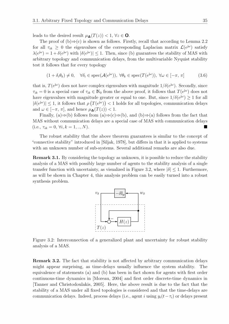
3.1. Arbitrary Fixed Topology and Communication Delays 35
leads to the desired result µ∆(T (z)) < 1, ∀z ∈ O.
The proof of (b)⇒(c) is shown as follows. Firstly, recall that according to Lemma 2.2
for all τik ≥ 0 the eigenvalues of the corresponding Laplacian matrix L(ejω) satisfy
λ(ejω) = 1 + δ(ejω) with |δ(ejω)| ≤ 1. Then, since (b) guarantees the stability of MAS with
arbitrary topology and communication delays, from the multivariable Nyquist stability
test it follows that for every topology
(1 + δiθk) 6= 0, ∀δi ∈ spec(A(ejω)), ∀θk ∈ spec(T (ejω)), ∀ω ∈ [−π, π] (3.6)
that is, T (ejω) does not have complex eigenvalues with magnitude 1/δ(ejω). Secondly, since
τik = 0 is a special case of τik ∈ N0 from the above proof, it follows that T (ejω) does not
have eigenvalues with magnitude greater or equal to one. But, since 1/δ(ejω) ≥ 1 for all
|δ(ejω)| ≤ 1, it follows that ρ(T (ejω)
)< 1 holds for all topologies, communication delays
and ω ∈ [−π, π], and hence µ∆(T (z)) < 1.
Finally, (a)⇒(b) follows from (a)⇒(c)⇒(b), and (b)⇒(a) follows from the fact that
MAS without communication delays are a special case of MAS with communication delays
(i.e., τik = 0, ∀i, k = 1, .., N). �
The robust stability that the above theorem guarantees is similar to the concept of
“connective stability” introduced in [Siljak, 1978], but differs in that it is applied to systems
with an unknown number of sub-systems. Several additional remarks are also due.
Remark 3.1. By considering the topology as unknown, it is possible to reduce the stability
analysis of a MAS with possibly large number of agents to the stability analysis of a single
transfer function with uncertainty, as visualized in Figure 3.2, where |δ| ≤ 1. Furthermore,
as will be shown in Chapter 4, this analysis problem can be easily turned into a robust
synthesis problem.
H(z)
−δIp
T (z)
wδvδ
−
Figure 3.2: Interconnection of a generalized plant and uncertainty for robust stability
analysis of a MAS.
Remark 3.2. The fact that stability is not affected by arbitrary communication delays
might appear surprising, as time-delays usually influence the system stability. The
equivalence of statements (a) and (b) has been in fact shown for agents with first order
continuous-time dynamics in [Moreau, 2004] and first order discrete-time dynamics in
[Tanner and Christodoulakis, 2005]. Here, the above result is due to the fact that the
stability of a MAS under all fixed topologies is considered and that the time-delays are
communication delays. Indeed, process delays (i.e., agent i using yi(t−τi) or delays present
36 Chapter 3. Robust Stability Analysis of Multi-Agent Systems
in the system model (2.1) as, e.g., in [Fax and Murray, 2004, Example 1]) will influence
the stability of the agents and of the MAS. Furthermore, although not influencing the
stability, the communication delays will in general affect the performance.
Finally, note that in the case of stability analysis of the information flow loop (Fig-
ure 2.6), one can write T (z) = R(z) since R(z) = (Ip + F (z))−1 F (z).
The above theorem provides a stability analysis condition for a MAS with arbitrary
topology and communication delays, by treating the topology as unknown/uncertain and
hence resulting in a robust stability condition. Clearly, since time-invariant topologies
are a special case of the time-varying ones, the above condition constitutes a necessary
condition for stability of MAS with time-varying topologies.
3.2 Switching Topology and Time-Varying Commu-
nication Delays
Although usually robust stability results can be easily generalized to obtain a sufficient
condition for stability under time-varying uncertainty, this cannot be simply done for multi-
agent systems. At the same time, as shown in [Wang and Elia, 2009a], the decomposition
approach proposed in [Fax and Murray, 2004] is not applicable to time-varying systems.
To see the latter consider a MAS with switching topology, but without communication
delays. Let the topology at time t be described by the Laplacian matrix L(t). Then the
autonomous dynamics of the MAS are described by:
x(t+ 1) =(A + BL(p)(t)C
)x(t),
where A, B, C are the system matrices of H(z), and A = IN⊗A, . . . . The decomposition ap-
proach from [Fax and Murray, 2004] requires now that a diagonalizing state transformation
is performed with x(t) = Q(nx)(t)x(t), where Q(nx) = Q⊗ Inx and Q(t)L(t)Q−1(t) = U(t),
where U is diagonal or upper triangular. Applying this transformation to the above
equation leads to
x(t+ 1) = Q−1(nx)(t+ 1)
(A + BL(p)(t)C
)Q(nx)(t)x(t).
However, as in general Q−1(t+ 1)Q(t) 6= IN , the above transformation does not result in a
diagonal or upper-triangular system matrix and hence, the decomposition result from [Fax
and Murray, 2004] does not hold. In order to avoid this problem here, an approach that
does not rely on the decomposition technique will be used.
Before proceeding, it is useful to recall the definitions of two system norms. Let G(z)
be a transfer function with p outputs and q inputs, G(z) =
A B
C D
, with Markov
parameters of its impulse response given by G(t). If u(t) is the input and y(t) the output of
the transfer function at time t, then the system norm induced by the infinity signal norm
(cf. [Dahleh and Ohta, 1988; Khammash and Pearson, 1991; Skogestad and Postlethwaite,
3.2. Switching Topology and Time-Varying Communication Delays 37
2005; Rieber, 2007]) is:
‖G(z)‖1 = supu(t)6=0
‖y(t)‖∞‖u(t)‖∞
= supu(t)6=0
‖∑th=0 G(h)u(t− h)‖∞‖u(t)‖∞
= maxi∈[1,p]
q∑k=1
∞∑h=0
|Gik(h)|,
where under u(t) 6= 0 it is meant that ∃t, such that u(t) 6= 0. The above expression is
called the system one norm (i.e., the l1 norm), as for SISO systems it is simply the one
norm of the coefficients of the impulse response. Furthermore, recall (see, e.g., [Skogestad
and Postlethwaite, 2005]) that the system norm induced by the signal two norm is the
H∞ norm:
‖G(z)‖∞ = supu(t)6=0
‖y(t)‖2
‖u(t)‖2
= supω∈[−π, π]u∈Cq , u 6=0
‖G(ejω)u‖‖u‖ = sup
ω∈[−π, π]
σ(G(ejω)
).
In the following it will be implicitly assumed that if due to a change in the topology an
agent receives the outputs of a neighbor from several different time steps, then only the
most recent output will be used. For example, if at time t agent i receives both yk(t− 3)
and yk(t− 5) then it will use only yk(t− 3).
The following theorem establishes a sufficient condition for the stability of a MAS
under a time-varying topology and communication delays.
Theorem 3.3. A multi-agent system of agents with transfer function H(z) is stable for
any number of agents N and any switching topology and time-varying communication
delays τik(t) ≥ 0, ∀i, k ∈ [1, N ],∀t, if there exists an invertible matrix D ∈ Rp×p, such that
‖DT (z)D−1‖1 < 1. (3.7)
Proof. As only the stability of the MAS is of interest, in the following it will be assumed
that the reference signal rik(t) = 0, ∀i, k, t. Then, for a communication topology with
time-invariant communication delays, one can write the error signal ei(t) (see (2.7) and
(2.8)) as
ei(t) = −yi(t) +1
|Ni(t)|∑
k∈Ni(t)
yk(t− τik)
= −yi(t) +t∑
h=0
1
|Ni(t)|∑
k∈Ni(t)τik≡h
yk(t− h),
where the upper bound of the sum over h can be replaced by τ = maxi,k
τik. In the above
equation the inner sum is over the outputs that are delayed by τik steps. For the error
signal e(t) of the overall MAS one can now write:
e(t) = −y(t)−t∑
h=0
Ahy(t− h), (3.8)
38 Chapter 3. Robust Stability Analysis of Multi-Agent Systems
where the matrices Ah are appropriately constructed, such that they select the neighbors
from which the agents receive information with delay of h steps. Alternatively, in z-domain
one could write e(z) =[−IpN −
∑τh=0 Ahz
−h]y(z).
In the case of a time-varying topology, the matrices Ah are also time-varying and
equation (3.8) can be rewritten as
e(t) = −y(t)−t∑
h=0
Ah(t)y(t− h) (3.9)
= −y(t)−A(p)(t)y(t),
where A(p)(t) is now an operator. By using that T (z) = (Ip + H(z))−1H(z) and
L(p)(t) = IpN +A(p)(t), one can rearrange as in Figure 3.1 by substituting wA(t) = y(t)
and vA(t) = −∑th=0Ah(t)y(t−h). Now the time-varying communication topology A(p)(t)
can be completely characterized by a pulse response matrix (see, e.g., [Khammash and
Pearson, 1991; Shamma and Dahleh, 1991]) in the following formvA(0)
vA(1)
vA(2)...
=
R00 0 0 0 . . .
R10 R11 0 0 . . .
R20 R21 R22 0...
......
.... . .
...
︸ ︷︷ ︸
y(0)
y(1)
y(2)...
︸ ︷︷ ︸
(3.10)
R y
where Rth = −At−h(t).With these definitions, it is easy to check that A(p)(t) : lpN∞ → lpN∞ and
‖A(p)‖1= sup
y∈lpN∞ \0
‖Ry‖∞‖y‖∞
= 1,
or in other words, A(p) maps bounded signals to bounded signals with the same infinity
norm. This follows from the construction of A(p)(t) from the Laplacian and can be seen
from the pulse response matrix R – because its elements are the elements of the normalized
adjacency matrix at that time, it follows that the sum of the absolute values of the elements
in each row of R is (not greater than) 1. The value of 1 is attained, for example, for an
undirected topology with 2 agents and no communication delays.
Now define a scaling matrix D = IN ⊗D, where D ∈ Rp×p is invertible, and note that
D−1A(p)D = A(p), since from the properties of the Kronecker product (see, e.g., [Brewer,
1978]) A(p)D = (A ⊗ Ip)(IN ⊗ D) = (IN ⊗ D)(A ⊗ Ip) = DA(p). Then, by applying the
small-gain theorem [Dahleh and Khammash, 1993, Theorem 2] (using the norm induced
by the signal infinity norm) to the feedback loop of T(z) and A(p) one obtains that a
sufficient condition for stability is
‖DT(z)D−1‖1 = ‖IN ⊗ (DT (z)D−1)‖1 = ‖DT (z)D−1‖1 < 1.
The last equality is obtained by exploiting that the norm, induced by the signal infinity
norm, is the maximal over the ones for the individual transfer functions DT (z)D−1, which
due to the replication are all equivalent. �
3.2. Switching Topology and Time-Varying Communication Delays 39
The above theorem reduces the stability analysis of a MAS with arbitrary time-
varying topology to analysis of the scaled l1 system norm of a single agent. The following
theorem shows that for MAS with symmetric Laplacian matrix, i.e., topology satisfying
L(ejω) = LT(ejω), the scaled l1 system norm condition can be exchanged with a scaled H∞condition.
Theorem 3.4. A multi-agent system of agents with transfer function H(z) is stable for any
number of agents N and any switching topology without communication delays(τik(t) = 0,
∀i, k ∈ [1, N ]) satisfying L(t) = LT(t), ∀t, if there exists an invertible matrix D ∈ Rp×p
such that the norm of DT (z)D−1, induced by the signal two norm, satisfies
‖DT (z)D−1‖∞ < 1. (3.11)
Proof. Since only symmetric topologies are considered, for the normalized adjacency
matrices holds A(t) = AT(t), ∀t. Recall that for any fixed t the eigenvalues of At = A(t)
satisfy |δi| ≤ 1. Let vi be a right eigenvector corresponding to δi. Since At is symmetric it
follows that vi is also a right eigenvector of ATt . Recall that the singular values of a matrix
At are the square root of the eigenvalues of ATt At. Then, since AT
t Atvi = ATt δivi = δ2
i vi,
it follows that the singular values σi of At are equal to√δ2i and hence satisfy |σi| ≤ 1,
∀i, t. Thus, the signal two induced norm of At is not greater than one. Then one can treat
A(t) as norm bounded time-varying uncertainty and apply the small gain theorem to the
interconnection of T(z) and A(p). By using the fact that a constant matrix D = IN ⊗D
commutes with A(p)(t) one obtains that the interconnection is stable if for some D ∈ Rp×p
‖DT(z)D−1‖∞ = ‖DT (z)D−1‖∞ < 1. (3.12)
The last equation has been obtained by using that the H∞ norm of a block-diagonal
system is the maximum of the H∞ norms of the transfer functions of the blocks on the
diagonal. �
A similar result, following a different line of proof and resulting in a non-scaled (i.e.,
more conservative) H∞ condition has been shown in [Wang and Elia, 2009a].
Remark 3.3. Unlike the previous two theorems, Theorem 3.4 does not allow for delays
in the information exchange between the agents. The reason for this is that an operator
transforming y(t) into y(t− τ(t)) does not necessary have a bounded signal two induced
norm, i.e., it can “generate” energy (cf. [Kao and Rantzer, 2005]). To see this consider a
MAS with two agents and undirected communication topology. The normalized adjacency
matrix is A =
[0 −1
−1 0
]. Consider that there is a communication-delay τ12 from agent
2 to agent 1 and that it is τ12(t) = t, ∀t. Let the input y(t) to A be y(0) =[0 1
]Tat
time 0 and zero for t > 0. Clearly the energy of y is ‖y(t)‖2 = 1. However for the output
of A one obtains v(t) =[1 0
]T, ∀t, which clearly makes the gain of A, induced by the
signal two norm, unbounded. Note, that this was not an issue in Theorem 3.3 since the
magnitude of v(t) remains unchanged (i.e., its infinity norm).
In order to address also topologies with time-varying delays in the information exchange
between the agents, one will need to consider the practical implications of time-varying
delays like the above. In fact, it is needed to analyze under what conditions an agent can
40 Chapter 3. Robust Stability Analysis of Multi-Agent Systems
• receive a signal yi(h− k) after it has received a signal yi(h), where k > 0, or
• reuse signal yi(h) at several time-steps t.
In order to facilitate the discussion, two cases can be distinguished.
1. Sensing topology - in this case the agents receive analog/digital signals about the
distances to the neighbors from an on-board sensor. As the sensor data are sampled
and “immediately” used, it is not possible to obtain a signal yi(h− k) after yi(h).
Reusing the same signal yi(h) at several time instances could then occur only, if in
case of signal loss (agents get outside of sensing range, sensor error, etc.) the agent
reuses the last obtained signal. Hence, in order to avoid such possibility, the agent
should remove agent i from its list of neighbors.
2. Communication topology - in this case an information message send from one agent
might be delayed in the communication network due to bandwidth limitations and
different routing of the different messages (e.g., consider agents communicating
over the Internet). However, as in this case the communication messages can be
augmented by a time-stamp, the agents can be made to “neglect” all messages with
earlier time-stamp than the newest received. Furthermore, it is not required for the
agents to share a common clock, as from the time-stamps of yi(h) and yi(h− k) an
agent will deduce the same chronological order as from the time-stamps of yi(t+ h)
and yi(t+ h− k). As before, in the case of communication “blackout”/“loss”, the
agents are not allowed to reuse a previously received signal.
These requirements can be described by an appropriate definition of a set τ ik of
sequences of time-varying communication delays from agent k to agent i. The delays are
iteratively defined (over t) as follows
τ ik :=
{τik(t)
∣∣∣∣ h(−1) = 0,if k ∈ Ni(t)⇒ τik(t) ∈ [0, h(t− 1)]; h(t) = τik(t)
if k /∈ Ni(t)⇒ h(t) = h(t− 1) + 1.
}In the above definition h(t) plays the role of slag variable, limiting the maximal allowed
communication-delay. As an extension of condition (3.12) to such topologies can be rather
involved and would address only special topology cases, it is not pursued further.
Remark 3.4. Unfortunately, Theorem 3.4 imposes an additional restriction compared to
Theorem 3.2 – it constraints the topologies to symmetric one, i.e., satisfying L = LT. This
restriction cannot be avoided by considering the complete closed-loop MAS and treating
A as bounded uncertainty, as its signal two induced norm is (generally) not less than one.
To see this, consider a MAS with 3 agents and a topology described by the Laplacian
L =
1 −0.5 −0.5
0 1 −1
0 −1 1
.The singular values of the corresponding normalized adjacency matrix A = L− I3 are 0, 1
and√
6/2 ≈ 1.22.
3.3. Computational Aspects 41
As already discussed, the decomposition approach of Fax and Murray [2004] cannot
be applied to this problem, due to the required time-varying transformation “matrix.”
However, it is interesting to note that if Theorem 2.3 could be applied to MAS with
time-varying topologies (i.e., the stability of the MAS could be equated to the simultaneous
stability of N agents under the time-varying “eigenvalues” of the Laplacian), one could
easily obtain an H∞ robust stability condition. This could be done by considering the
time-varying eigenvalues of A as bounded uncertainty δIp, since they remain inside the
unit disk for all topologies and communication delays, and using that for time-varying
structured uncertainty one needs to exchange the structured singular value with
infD∈Rp×p
σ(DT (ejω)D−1).
Moreover, if such analysis was possible, one could use a result obtained in [Shamma, 1994,
Theorem 3.1], which by requiring that τik > 0, ∀i, k ∈ [1, N ] would render (3.11) both
a necessary and sufficient condition for stability. The condition on τik simply requires
that there is at least one time-step delay in the communication (which is satisfied for all
physical systems) and allows treating the uncertainty δIp as a dynamical one. For further
discussion on parametric uncertainty and the difference that τik = 0 makes, the reader is
referred to [Iwasaki, 1997].
3.3 Computational Aspects
The stability analysis of a MAS using Theorem 3.2 requires verifying that condition
(3.2) holds. Because of the structure of ∆ = δIp this is equivalent to the condition
supω∈[0, π]
ρ(T (ejω)
)< 1, which is a well known robust stability problem (cf. [Skogestad and
Postlethwaite, 2005; Balas et al., 2001]), but which cannot be (in general) analytically
verified. An usual approach is to perform a frequency sweep, by which ρ(T (ejω)
)is checked
only on selected frequencies. Unfortunately, this can provide only a lower bound as sharp
peaks in µ∆(T (z)) might not be detected. An alternative is to exchange µ∆(T (z)) with an
upper bound ‖D(z)T (z)D−1(z)‖∞, where D(z) is a bi-proper, invertible dynamic system
with p inputs and p outputs [Balas et al., 2001]. However, as in many cases one would be
interested in the stability under a time-varying topology the details are omitted.
For the stability analysis with Theorem 3.3, one needs to find an invertible D ∈ Rp
matrix, such that the one norm of the impulse response of DT (z)D−1 is smaller than one.
One can distinguish between two cases p = 1 and p > 1. In the former case, the stability
condition (3.7) reduces to ‖T (z)‖1 < 1. In other words, one needs to verify whether the
one norm of the Markov parameters of the impulse response, i.e.,
‖T (z)‖1 = maxi∈[1,p]
p∑k=1
∞∑h=0
|Tik(h)| =∞∑h=0
|T (h)|,
is smaller than one. However, this can be exactly computed only for systems with finite
impulse response. In general, one can obtain a lower bound ϑg (cf. [Rieber, 2007]) of the
42 Chapter 3. Robust Stability Analysis of Multi-Agent Systems
above expression as:
‖T (z)‖1 = maxi∈[1,p]
p∑k=1
g∑h=0
|Tik(h)|︸ ︷︷ ︸+ maxi∈[1,p]
p∑k=1
∞∑h=g+1
|Tik(h)|︸ ︷︷ ︸ .ϑg ϑr,g
However, since a lower bound does not guarantee that the stability condition is satisfied,
one needs to find an upper bound of ‖T (z)‖1 instead. The following theorem is based on
the star-norm upper bound of the l1-norm (or upper bound of ϑr,g) provided in [Rieber,
2007, Theorem 2.1]. Let
T (z) =
A B
C D
has n states, p inputs and p outputs.
Theorem 3.5. The inequality ‖T (z)‖1 < ϑ√p is satisfied if there exist β1 > 0, β2 ∈ (0, 1)
and a symmetric matrix X ∈ Cn×n, such that−ATXA− β2X −ATXB 0 0 0
• −BTXB + β1Ip 0 0 0
• • (1− β2)X 0 CT
• • • (ϑ2 − β1)Ip DT
• • • • Ip
� 0. (3.13)
This cannot be posed as an Linear Matrix Inequality (LMI) problem due to the product
of β2 and X. However, one could solve it, for example, by iteratively fixing X and β1 and
solving for β2 and then fixing β2 and solving for X and β1.
In the case p > 1, one needs to apply Theorem 3.5 to the system
DT (z)D−1 =
A BD−1
DC DDD−1
.This will result in matrix inequality that contains also terms with products of X and D.
However, one can perform a congruence transformation with U = diag(In, DT, In, DT, DT
)as left and UT as right factor and substitute DTD = S � 0. Then the inequality
‖DT (z)D−1‖1 < ϑ√p will be satisfied if there exist β1 > 0, β ∈ (0, 1) and symmetric
matrices X ∈ Cn×n and S ∈ Cp×p such that−ATXA− β2X −ATXB 0 0 0
• −BTXB + β1S 0 0 0
• • (1− β2)X 0 CTS
• • • (ϑ2 − β1)S DTS
• • • • S
� 0. (3.14)
As this feasibility problem contains product of variables (β2X and β1S) it is a Bi-Linear
Matrix Inequality (BMI) and cannot be solved directly. An overview of several methods for
3.3. Computational Aspects 43
attacking such kind of problems (among which the above mentioned iterative procedure)
is provided in Chapter 5.
In the stability analysis with Theorem 3.4, one can again distinguish between the cases
p = 1 and p > 1. In the former case, the condition (3.11) reduces to the standard H∞stability condition ‖T (z)‖∞ < 1. This can be readily verified via state of the art robust
analysis tools such as the computation of the H∞ norm (e.g. [Bruinsma and Steinbuch,
1990]) or using the following theorem.
Theorem 3.6 ([D’Oliveira et al., 1999, Theorem 2]). The inequality ‖T (z)‖∞ < γδ is
satisfied if and only if there exist a matrix X ∈ Cn×n and a symmetric matrix P ∈ Cn×nsuch that
P AX B 0
• X +XT − P 0 (CX)T
• • Ip DT
• • • γ2δ Ip
� 0 (3.15)
is satisfied.
For γδ = 1 this is an LMI feasibility problem in P and X.
In the case p > 1, the stability condition can be expressed as an LMI condition in D
for a fixed frequency [Packard and Doyle, 1993]. This is however not practical for dynamic
systems, as it requires checking the condition at infinitely many frequencies simultaneously.
At the same time, using the upper bound ‖T (z)‖∞ < 1 results in a conservative condition
for stability.
Alternatively, applying Theorem 3.6 to the system DT (z)D−1 results in a matrix
inequality containing product of variables. Similarly to the approach used in [Apkairan
and Adams, 2000], one can perform a congruence transformation with U as left and UT
as right factor, where U = diag (In, In, D−1, D−1), and substitute S = D−1D−T � 0. This
allows one to replace the search for a D ∈ Rp×p satisfying ‖DT (z)D−1‖∞ < 1 with a search
for a matrix X ∈ Cn×n, a symmetric P ∈ Cn×n and a positive definite matrix S ∈ Cp×p,S1 = S2 = S, such that
P AX BS1 0
• X +XT − P 0 (CX)T
• • S1 S1DT
• • • γ2δS2
� 0 (3.16)
is satisfied for γδ = 1. This is an LMI feasibility problem equivalent to (3.11), for which
efficient interior point methods exist [Boyd and Vandenberghe, 2004]. The reason for
introducing separate S1 and S2 will become clear later on.
It should be remarked, that an approximation of the minimal value of γδ, for which the
above inequality is satisfied, can be computed as well, e.g., by solving the above problem
iteratively using a bisection technique for γ2δ . However, the corresponding scaling factor
cannot be obtained, as the decision variable is S = (DTD)−1, which does not have a unique
solution for D ∈ Rp×p. An alternative approach, based on gradient-based search over D,
that can return the D matrix, will be presented in Chapter 5.2.
44 Chapter 3. Robust Stability Analysis of Multi-Agent Systems
Example 3.1. Consider a cooperative control of hovercrafts as in Example 2.1, with
local controllers as in Example 2.4 and a closed-loop MAS as in Figure 2.3. Such a MAS
will not be stable under arbitrary topologies, as the inequality in (3.16) has no feasible
solution for γδ < 1.0584. In fact, since T (z) is a SISO transfer function ∆ = δ and also
µ∆(T (z)) = 1.0584. The fact that the MAS is not stable under arbitrary topologies
can be graphically confirmed from the Nyquist plot in Example 2.4, since the Nyquist
diagram of H(z) crosses the −0.5 line. An example topology, for which such a MAS
is unstable, is a cyclic interconnection of N = 4 agents without communication delays,
where Ni = i+ 1, i = 1, 2, 3 and N4 = 1. A lower bound for the l1 norm of this system
is ϑ1000 ≈ 1.2756.
3.4 Areas of Application
Depending on the available knowledge about a multi-agent system, one could roughly
distinguish between the following cases:
C1 Fixed and known topology and communication-delays;
C2 Unknown but fixed topology and communication delays;
C3 Switching topology and time-varying communication delays.
Clearly, in case C1 and for τik = 0, ∀i, k ∈ [1, N ], one can analyze the stability of the
MAS using the decomposition result from Theorem 2.3. This is however not applicable
when τik 6= 0 as then the eigenvalues are frequency dependent. In this case, one has to
analyze the stability of the transfer function S(z) of the MAS directly (see eq. (2.11)).
In the case C2 of time-invariant but unknown topology and communication delay, the
stability analysis reduces to the one in Theorem 3.2. It is interesting to note that in
the case of no communication delays, one could also apply the decomposition approach
proposed in [Massioni and Verhaegen, 2009; Massioni, 2010]. In that case one has to check
the simultaneous feasibility with a fixed Lyapunov matrix of LMIs corresponding to the
transfer functions Pλi obtained after a decomposition (see Theorem 2.3), where λi are the
vertices of a convex hull C, such that P ∈ C. However, this can be performed only at the
price of overbounding and increased computational cost. For example, by approximating
the Perron disk by a square with vertices 0± j1 and 2± j1 one has a system of 4 LMIs (i.e.,
four-times the size of the LMI in (3.16)) accompanied by a significant conservatism due to
considering areas not belonging to the Perron disk. This conservatism can be reduced by
increasing the number of vertices, but at the price of increased problem size.
Finally, in the extreme case of switching topology and time-varying communication
delays the stability of a MAS can be verified by means of Theorems 3.3–3.4, i.e., conditions
(3.14) and (3.16).
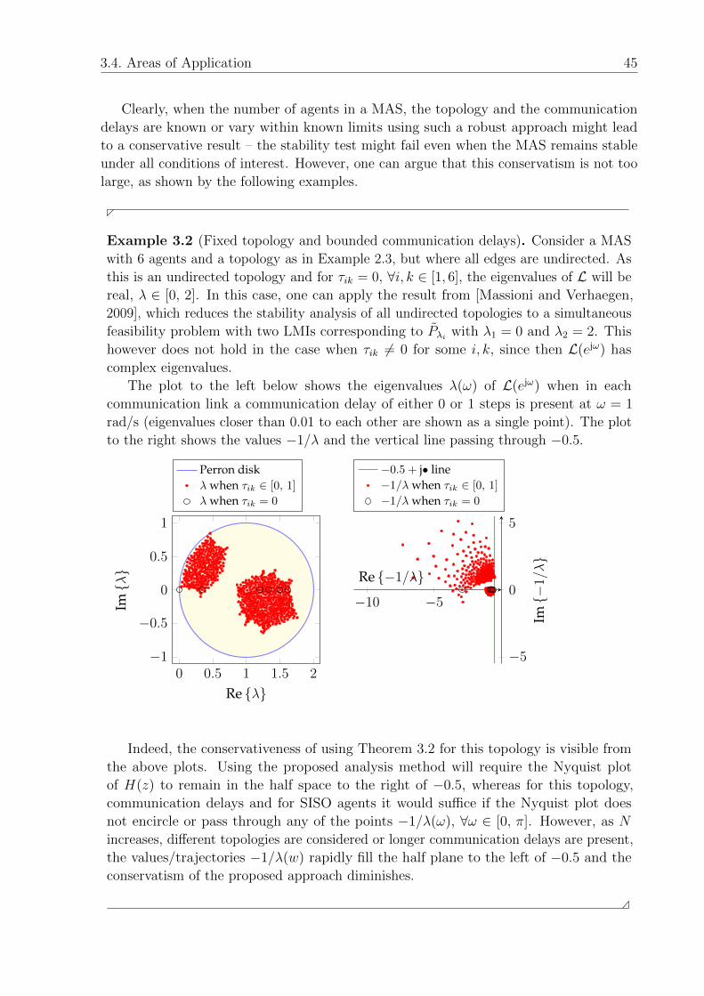
3.4. Areas of Application 45
Clearly, when the number of agents in a MAS, the topology and the communication
delays are known or vary within known limits using such a robust approach might lead
to a conservative result – the stability test might fail even when the MAS remains stable
under all conditions of interest. However, one can argue that this conservatism is not too
large, as shown by the following examples.
Example 3.2 (Fixed topology and bounded communication delays). Consider a MAS
with 6 agents and a topology as in Example 2.3, but where all edges are undirected. As
this is an undirected topology and for τik = 0, ∀i, k ∈ [1, 6], the eigenvalues of L will be
real, λ ∈ [0, 2]. In this case, one can apply the result from [Massioni and Verhaegen,
2009], which reduces the stability analysis of all undirected topologies to a simultaneous
feasibility problem with two LMIs corresponding to Pλi with λ1 = 0 and λ2 = 2. This
however does not hold in the case when τik 6= 0 for some i, k, since then L(ejω) has
complex eigenvalues.
The plot to the left below shows the eigenvalues λ(ω) of L(ejω) when in each
communication link a communication delay of either 0 or 1 steps is present at ω = 1
rad/s (eigenvalues closer than 0.01 to each other are shown as a single point). The plot
to the right shows the values −1/λ and the vertical line passing through −0.5.
0 0.5 1 1.5 2−1
−0.5
0
0.5
1
Re {λ}
Im{λ}
Perron diskλ when τik ∈ [0, 1]
λ when τik = 0
−10 −5
−5
0
5
Re {−1/λ}
Im{−
1/λ}
−0.5 + j• line−1/λ when τik ∈ [0, 1]
−1/λ when τik = 0
Indeed, the conservativeness of using Theorem 3.2 for this topology is visible from
the above plots. Using the proposed analysis method will require the Nyquist plot
of H(z) to remain in the half space to the right of −0.5, whereas for this topology,
communication delays and for SISO agents it would suffice if the Nyquist plot does
not encircle or pass through any of the points −1/λ(ω), ∀ω ∈ [0, π]. However, as N
increases, different topologies are considered or longer communication delays are present,
the values/trajectories −1/λ(w) rapidly fill the half plane to the left of −0.5 and the
conservatism of the proposed approach diminishes.
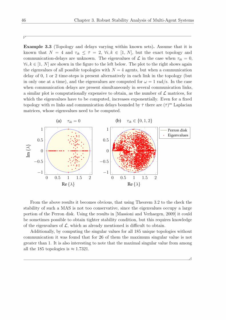
46 Chapter 3. Robust Stability Analysis of Multi-Agent Systems
Example 3.3 (Topology and delays varying within known sets). Assume that it is
known that N = 4 and τik ≤ τ = 2, ∀i, k ∈ [1, N ], but the exact topology and
communication-delays are unknown. The eigenvalues of L in the case when τik = 0,
∀i, k ∈ [1, N ] are shown in the figure to the left below. The plot to the right shows again
the eigenvalues of all possible topologies with N = 4 agents, but when a communication
delay of 0, 1 or 2 time-steps is present alternatively in each link in the topology (but
in only one at a time), and the eigenvalues are computed for ω = 1 rad/s. In the case
when communication delays are present simultaneously in several communication links,
a similar plot is computationally expensive to obtain, as the number of L matrices, for
which the eigenvalues have to be computed, increases exponentially. Even for a fixed
topology with m links and communication delays bounded by τ there are (τ)m Laplacian
matrices, whose eigenvalues need to be computed.
0 0.5 1 1.5 2−1
−0.5
0
0.5
1
Re {λ}
Im{λ}
(a) τik = 0
0 0.5 1 1.5 2−1
−0.5
0
0.5
1
Re {λ}
(b) τik ∈ {0, 1, 2}
Perron diskEigenvalues
From the above results it becomes obvious, that using Theorem 3.2 to the check the
stability of such a MAS is not too conservative, since the eigenvalues occupy a large
portion of the Perron disk. Using the results in [Massioni and Verhaegen, 2009] it could
be sometimes possible to obtain tighter stability condition, but this requires knowledge
of the eigenvalues of L, which as already mentioned is difficult to obtain.
Additionally, by computing the singular values for all 185 unique topologies without
communication it was found that for 26 of them the maximum singular value is not
greater than 1. It is also interesting to note that the maximal singular value from among
all the 185 topologies is ≈ 1.7321.
3.4. Areas of Application 47
From the above discussion and examples it should be clear, that in many cases applying
the proposed robust technique to the stability analysis of a MAS is conservative, but
at the same time it is often the only feasible approach. In fact, in some cases this
conservatism might be desired. For example, in MAS with a large number of agents or
MAS whose topology is often subjected to disturbances/communication obstacles, this
approach allows one to account for changes in the topology and for communication delays.
Indeed, treating the communication topology as unknown allows to avoid problems, like
the one demonstrated in [Fax and Murray, 2004], where an additional communication
channel between 2 agents causes instability of the MAS.
In the remainder of this thesis the focus will be on controller and information filter
synthesis based on the scaled H∞ condition from Theorem 3.4. The scaled l1-condition
from Theorem 3.3 will be used as an a posteriori condition to verify the robust stability
under time-varying topologies. There are several reasons for focusing on the H∞ problem,
rather than on the l1 problem.
• The scaled H∞ condition (3.11) represents an upper bound on the structured singular
value condition in (3.2). That is, by satisfying (3.11) the stability of a MAS with an
arbitrary time-invariant topology is guaranteed.
• In contrast to (3.16), which is both necessary and sufficient for ‖DT (z)D−1‖∞ < 1,
the condition (3.14) provides only a sufficient condition for ‖DT (z)D−1‖1 < 1 (i.e.,
an upper bound of the l1 norm), and furthermore cannot be efficiently verified.
• As in many cases the communication topology does not change arbitrary fast, the
fact that the scaled H∞ condition is an upper bound on the µ∆ condition will suffice
for guaranteeing acceptable system behaviour.
• It is possible to express an upper bound of the system l1-norm by an appropriately
scaled H∞ norm [Boyd and Doyle, 1987; Venkatesh and Dahleh, 1994].
• As it will be shown in the following chapter, the scaled H∞ approach results in an
efficient synthesis method for a MAS with directed communication topology and
communication delays.
• In many cases a controller that satisfies eq. (3.11) will also satisfy eq. (3.7).
Publications
A small-gain sufficient condition for stability of a MAS under arbitrary fixed topology
without communication delays has been published in [Popov and Werner, 2009]. An
improved sufficient condition for stability using the scaled H∞ condition in (3.11) has
appeared in [Pilz et al., 2009]. The presented in Theorems 3.2–3.4 necessary and sufficient
conditions for stability are publication in [Popov and Werner, 2012].

This page is intentionally left blank for pagination.
Chapter 4
Controller and Filter Synthesis
Techniques
New systems generate new problems.
Murphy’s law
In this chapter, the problem of designing a robust controller or a robust information-flow
filter will be addressed. The following set of basic design requirements on a controller
K(z) or an information-flow filter F (z) is considered.
R1 A MAS should remain stable for any number of agents, for arbitrary topology or
under switching topology and time-varying communication delays;
R2 If requirements on the agents and the connectivity of the topology are satisfied, such
as the ones imposed in [Moreau, 2005; Lee and Spong, 2006] or [Wang and Elia,
2009b], then the agents should reach consensus or output consensus, respectively;
R3 The agents and the MAS should satisfy performance requirements imposed by
selected frequency response shaping filters;
R4 The controller or the information-flow filter should be of a low-order or a fixed-
structure, i.e., K(z) ∈ K(z) and F (z) ∈ F(z), where K(z) and F(z) are the sets of
controllers and filters with the desired structural restrictions.
Note that the cooperative control requirement, i.e., that the vehicles are controlled in a
decentralized manner – by local on-board controllers, is assumed implicitly. Clearly, this
list can be extended by additional requirements such as constraints on the communication
channels, collision avoidance, etc., but these are outside the scope of this work.
In order to satisfy requirement R1 one needs to verify that Theorem 3.3 holds. However,
as discussed in Chapter 3, the associated scaled l1 problem is difficult to solve, and thus
not well suited for synthesis. Hence, the following two-step synthesis approach will be
applied instead.
1. The requirements R2 and R3 are addressed by formulating and solving an appropri-
ately defined scaled H∞ synthesis problem.
49
50 Chapter 4. Controller and Filter Synthesis Techniques
2. The condition from Theorem 3.3 is applied to the resulting system to verify that
requirement R1 is satisfied.
As the necessary computations for the a posteriori check of the scaled l1 condition from
(3.7) are discussed in Section 3.3, in this chapter the focus is on the first step of the
above approach. It is shown, that requirements R2 and R3 can be addressed as an
appropriately defined scaled H∞ design problem, which, however, cannot be solved using
standard synthesis tools. A solution to this problem, using the same techniques as in the
fixed-structure synthesis problem, will be presented in the following chapter.
4.1 Robust Stability Synthesis
As discussed in Chapters 2 and 3, problem P1 (see page 29) is important as a MAS is often
subject to changing topology due to obstacles, varying distances between the agents and
the particular task, since communication delays depend on reliability of communication
channels, bandwidth limitations, etc., and since for MAS with many agents the exact
topology and communication delays might not be precisely known. Theorems 3.2 and
3.4 reduce the stability analysis of such a MAS, to an analysis of a single agent with
uncertainty and could be easily reformulated for the purpose of controller/filter synthesis.
4.1.1 Information-Flow Filter Synthesis
Before addressing the robust synthesis of an information-flow filter, two remarks
should be made.
Remark 4.1. Recall that the local-loop controller C(z), by the consensus-based coop-
erative vehicle approach (Figure 2.6), can be designed independently of the information
filter, e.g., using H∞ or H2 synthesis techniques. However, designing a local controller of
a fixed-structure, i.e., C(z) ∈ C(z), belongs to problem P4 and will be addressed in the
following chapter. For the moment, assume that a controller C(z), stabilizing the vehicle
dynamics, is provided.
Remark 4.2. Note that in general the p information channels represent different physical
quantities and are not coupled to each other. This allows treating them independently, i.e.,
reducing the synthesis of a MIMO filter F (z) to the synthesis of p SISO filters F1(z), and
then constructing F (z) = Ip ⊗ F1(z). It is, additionally, possible to synthesize different
SISO filters Fh(z), h = 1, . . . , p, for the different channels and construct the overall filter
as F (z) = diag(F1(z), . . . , Fp(z)).
Let GF (z) be such that FL(GF (z), F1(z)) corresponds to T (z) in Figure 3.2 for p = 1.
The interconnection of GF (z) =
[0 1
J(z) −J(z)
]with the filter F1(z) is shown in Figure 4.1,
where vδ = −δwδ, δ ∈ Θ and J(z) = 1 (this block will be used later to satisfy requirement
R2). The subscript J is used to indicate that the corresponding signal is obtained by
passing through the block J(z), e.g., ˜J = J(z)˜, where for Figure 4.1: ˜= vδ − ξ.
Then, in order to synthesize an information filter F (z) = Ip ⊗ F1(z) satisfying the
condition in Theorem 3.4, one will have to solve the following design problem.
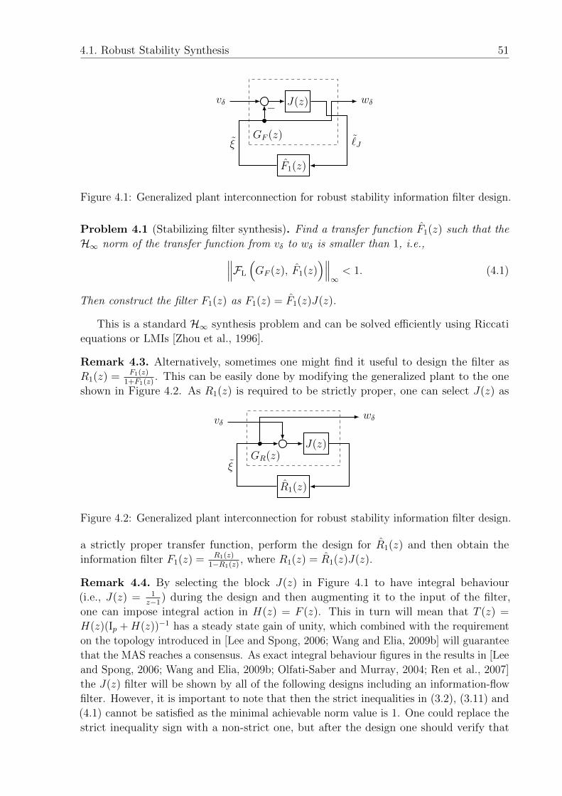
4.1. Robust Stability Synthesis 51
J(z)
F1(z)
wδvδ
GF (z) ˜Jξ
−
Figure 4.1: Generalized plant interconnection for robust stability information filter design.
Problem 4.1 (Stabilizing filter synthesis). Find a transfer function F1(z) such that the
H∞ norm of the transfer function from vδ to wδ is smaller than 1, i.e.,∥∥∥FL
(GF (z), F1(z)
)∥∥∥∞< 1. (4.1)
Then construct the filter F1(z) as F1(z) = F1(z)J(z).
This is a standard H∞ synthesis problem and can be solved efficiently using Riccati
equations or LMIs [Zhou et al., 1996].
Remark 4.3. Alternatively, sometimes one might find it useful to design the filter as
R1(z) = F1(z)1+F1(z)
. This can be easily done by modifying the generalized plant to the one
shown in Figure 4.2. As R1(z) is required to be strictly proper, one can select J(z) as
J(z)
R1(z)
GR(z)
wδvδ
ξ
Figure 4.2: Generalized plant interconnection for robust stability information filter design.
a strictly proper transfer function, perform the design for R1(z) and then obtain the
information filter F1(z) = R1(z)1−R1(z)
, where R1(z) = R1(z)J(z).
Remark 4.4. By selecting the block J(z) in Figure 4.1 to have integral behaviour
(i.e., J(z) = 1z−1
) during the design and then augmenting it to the input of the filter,
one can impose integral action in H(z) = F (z). This in turn will mean that T (z) =
H(z)(Ip +H(z))−1 has a steady state gain of unity, which combined with the requirement
on the topology introduced in [Lee and Spong, 2006; Wang and Elia, 2009b] will guarantee
that the MAS reaches a consensus. As exact integral behaviour figures in the results in [Lee
and Spong, 2006; Wang and Elia, 2009b; Olfati-Saber and Murray, 2004; Ren et al., 2007]
the J(z) filter will be shown by all of the following designs including an information-flow
filter. However, it is important to note that then the strict inequalities in (3.2), (3.11) and
(4.1) cannot be satisfied as the minimal achievable norm value is 1. One could replace the
strict inequality sign with a non-strict one, but after the design one should verify that
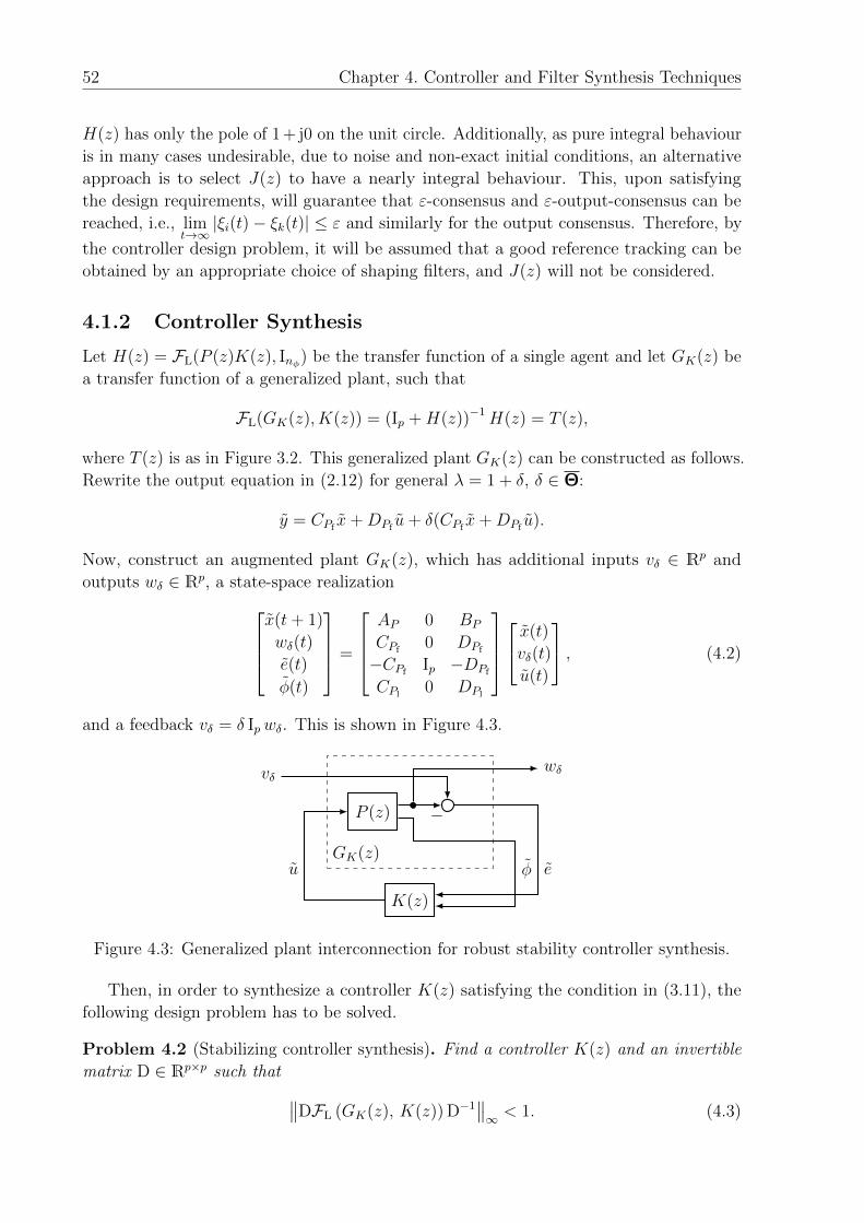
52 Chapter 4. Controller and Filter Synthesis Techniques
H(z) has only the pole of 1 + j0 on the unit circle. Additionally, as pure integral behaviour
is in many cases undesirable, due to noise and non-exact initial conditions, an alternative
approach is to select J(z) to have a nearly integral behaviour. This, upon satisfying
the design requirements, will guarantee that ε-consensus and ε-output-consensus can be
reached, i.e., limt→∞|ξi(t)− ξk(t)| ≤ ε and similarly for the output consensus. Therefore, by
the controller design problem, it will be assumed that a good reference tracking can be
obtained by an appropriate choice of shaping filters, and J(z) will not be considered.
4.1.2 Controller Synthesis
Let H(z) = FL(P (z)K(z), Inφ) be the transfer function of a single agent and let GK(z) be
a transfer function of a generalized plant, such that
FL(GK(z), K(z)) = (Ip +H(z))−1H(z) = T (z),
where T (z) is as in Figure 3.2. This generalized plant GK(z) can be constructed as follows.
Rewrite the output equation in (2.12) for general λ = 1 + δ, δ ∈ Θ:
y = CPfx+DPf
u+ δ(CPfx+DPf
u).
Now, construct an augmented plant GK(z), which has additional inputs vδ ∈ Rp and
outputs wδ ∈ Rp, a state-space realizationx(t+ 1)
wδ(t)
e(t)
φ(t)
=
AP 0 BP
CPf0 DPf
−CPfIp −DPf
CPl0 DPl
x(t)
vδ(t)
u(t)
, (4.2)
and a feedback vδ = δ Ipwδ. This is shown in Figure 4.3.
P (z)
K(z)
vδwδ
−
φ euGK(z)
Figure 4.3: Generalized plant interconnection for robust stability controller synthesis.
Then, in order to synthesize a controller K(z) satisfying the condition in (3.11), the
following design problem has to be solved.
Problem 4.2 (Stabilizing controller synthesis). Find a controller K(z) and an invertible
matrix D ∈ Rp×p such that ∥∥DFL (GK(z), K(z)) D−1∥∥∞ < 1. (4.3)
4.1. Robust Stability Synthesis 53
This is a scaledH∞ synthesis problem. It cannot be solved using standardH∞ synthesis
tools, such as Riccati equations or LMIs, since it contains product of decision variables.
One approach to attack this problem is to neglect the scalings and solve the corresponding
H∞ problem, i.e., finding K(z) s.t. ‖FL (GK(z), K(z))‖∞ < 1. This is however equivalent
to considering the set {X | X ∈ Cp×p, ‖X‖∞ ≤ 1} rather than δIp, δ ∈ Θ, which leads
to a conservative result. That is, a controller might not be found even if a solution
to Problem 4.2 exists. Therefore, the problem is typically attacked using an iterative
approaches such as D-K synthesis [Zhou et al., 1996] or S-K synthesis [Apkairan and
Adams, 2000] with static scaling matrices. Unfortunately, as the resulting problems are
convex in either of the variables but not jointly-convex, the iterative algorithms cannot
guarantee even convergence to a local minimum. An alternative approach, treating the
problem as a special case of a fixed-structure synthesis and optimizing simultaneously
over controller and scaling, is proposed in Section 5.2. Indeed, one can easily construct
a generalized plant GK(z) and a structured controller K(z) = diag(K(z), D−1, D), such
that FL(GK(z), K(z)) = DFL(GK(z), K(z))D−1.
Remark 4.5. The problem complexity depends on p and can, in some cases, be reduced.
For example, if for some q < p one can find matrices Dw ∈ Rp×q, Cz ∈ Rq×n, Dz ∈ Rq×b,
such that Dw
[Cz Dz
]=[CPf
DPf
]holds (e.g., by factoring
[CPf
DPf
]via singular-
value decomposition), one can rewrite GK(z) asx(t+ 1)
wδ(t)
e(t)
φ(t)
=
AP 0 BP
Cz 0 Dz
−CPfDw −DPf
CPl0 DPl
x(t)
vδ(t)
u(t)
,with a feedback vδ = δ Iq wδ. This in turn will require a search for an invertible Dq×q
matrix. In the limit, when q = 1, the scaled H∞ problem reduces to the standard H∞problem and can be solved efficiently. In fact, in the case when the agents communicate
the outputs yi, the same approach can be used to reduce the number of communicated
signals. In the following it will be assumed that if possible such transformation has been
performed and p = q holds.
Remark 4.6. Both of the above synthesis problems could have a trivial solution. In
the information-flow filter synthesis case this is F (z) = 0, which corresponds to no
communication exchange between the agents, in which case the local controllers guarantee
the overall stability. In the controller synthesis case, there can exist a trivial controller
with BKf= 0 and DKf
= 0, such that the stability of H(z) is guaranteed (i.e., the stability
of a single agent). In such a case, the agents will be stable but will not use the received
information from their neighbors, hence a MAS will remain stable independent on the
topology and communication delays. Therefore, in order to obtain a feedback-controller or
an information-flow filter, that not only guarantees the stability of the group of agents,
but allows them to achieve a certain task (trajectory following, formation acquisition,
etc.), one needs to impose additional performance requirements (e.g., in terms of speed
of convergence of the formation-level error). This problem is addressed in the following
section.
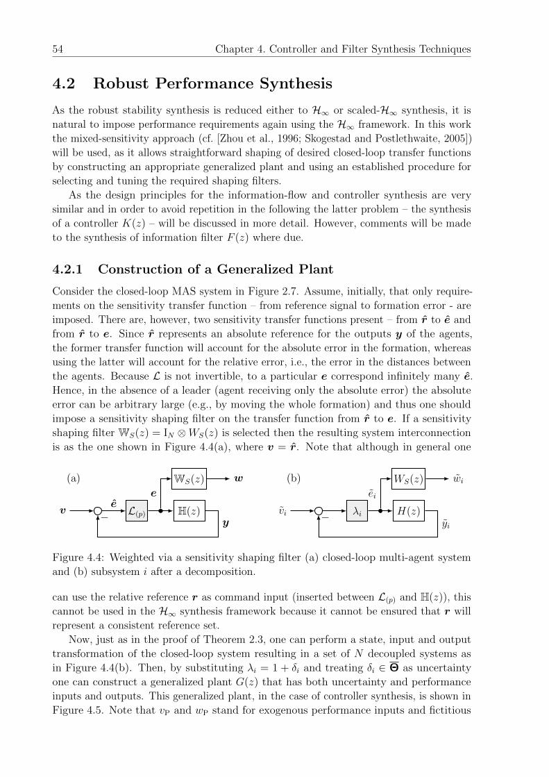
54 Chapter 4. Controller and Filter Synthesis Techniques
4.2 Robust Performance Synthesis
As the robust stability synthesis is reduced either to H∞ or scaled-H∞ synthesis, it is
natural to impose performance requirements again using the H∞ framework. In this work
the mixed-sensitivity approach (cf. [Zhou et al., 1996; Skogestad and Postlethwaite, 2005])
will be used, as it allows straightforward shaping of desired closed-loop transfer functions
by constructing an appropriate generalized plant and using an established procedure for
selecting and tuning the required shaping filters.
As the design principles for the information-flow and controller synthesis are very
similar and in order to avoid repetition in the following the latter problem – the synthesis
of a controller K(z) – will be discussed in more detail. However, comments will be made
to the synthesis of information filter F (z) where due.
4.2.1 Construction of a Generalized Plant
Consider the closed-loop MAS system in Figure 2.7. Assume, initially, that only require-
ments on the sensitivity transfer function – from reference signal to formation error - are
imposed. There are, however, two sensitivity transfer functions present – from r to e and
from r to e. Since r represents an absolute reference for the outputs y of the agents,
the former transfer function will account for the absolute error in the formation, whereas
using the latter will account for the relative error, i.e., the error in the distances between
the agents. Because L is not invertible, to a particular e correspond infinitely many e.
Hence, in the absence of a leader (agent receiving only the absolute error) the absolute
error can be arbitrary large (e.g., by moving the whole formation) and thus one should
impose a sensitivity shaping filter on the transfer function from r to e. If a sensitivity
shaping filter WS(z) = IN ⊗WS(z) is selected then the resulting system interconnection
is as the one shown in Figure 4.4(a), where v = r. Note that although in general one
WS(z) w
v L(p) H(z)e
y
e
(a)
−
WS(z) wi
vi λi H(z)yi
ei
(b)
−
Figure 4.4: Weighted via a sensitivity shaping filter (a) closed-loop multi-agent system
and (b) subsystem i after a decomposition.
can use the relative reference r as command input (inserted between L(p) and H(z)), this
cannot be used in the H∞ synthesis framework because it cannot be ensured that r will
represent a consistent reference set.
Now, just as in the proof of Theorem 2.3, one can perform a state, input and output
transformation of the closed-loop system resulting in a set of N decoupled systems as
in Figure 4.4(b). Then, by substituting λi = 1 + δi and treating δi ∈ Θ as uncertainty
one can construct a generalized plant G(z) that has both uncertainty and performance
inputs and outputs. This generalized plant, in the case of controller synthesis, is shown in
Figure 4.5. Note that vP and wP stand for exogenous performance inputs and fictitious
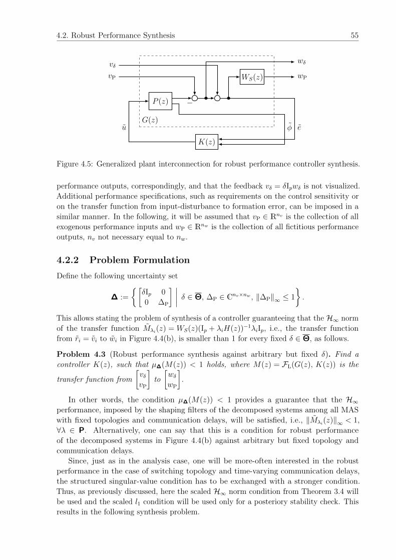
4.2. Robust Performance Synthesis 55
WS(z)
P (z)
K(z)
−
vδ
vP
wδ
wP
φ euG(z)
Figure 4.5: Generalized plant interconnection for robust performance controller synthesis.
performance outputs, correspondingly, and that the feedback vδ = δIpwδ is not visualized.
Additional performance specifications, such as requirements on the control sensitivity or
on the transfer function from input-disturbance to formation error, can be imposed in a
similar manner. In the following, it will be assumed that vP ∈ Rnv is the collection of all
exogenous performance inputs and wP ∈ Rnw is the collection of all fictitious performance
outputs, nv not necessary equal to nw.
4.2.2 Problem Formulation
Define the following uncertainty set
∆ :=
{[δIp 0
0 ∆P
] ∣∣∣∣ δ ∈ Θ, ∆P ∈ Cnv×nw , ‖∆P‖∞ ≤ 1
}.
This allows stating the problem of synthesis of a controller guaranteeing that the H∞ norm
of the transfer function Mλi(z) = WS(z)(Ip + λiH(z))−1λiIp, i.e., the transfer function
from ri = vi to wi in Figure 4.4(b), is smaller than 1 for every fixed δ ∈ Θ, as follows.
Problem 4.3 (Robust performance synthesis against arbitrary but fixed δ). Find a
controller K(z), such that µ∆(M(z)) < 1 holds, where M(z) = FL(G(z), K(z)) is the
transfer function from
[vδvP
]to
[wδwP
].
In other words, the condition µ∆(M(z)) < 1 provides a guarantee that the H∞performance, imposed by the shaping filters of the decomposed systems among all MAS
with fixed topologies and communication delays, will be satisfied, i.e., ‖Mλi(z)‖∞ < 1,
∀λ ∈ P. Alternatively, one can say that this is a condition for robust performance
of the decomposed systems in Figure 4.4(b) against arbitrary but fixed topology and
communication delays.
Since, just as in the analysis case, one will be more-often interested in the robust
performance in the case of switching topology and time-varying communication delays,
the structured singular-value condition has to be exchanged with a stronger condition.
Thus, as previously discussed, here the scaled H∞ norm condition from Theorem 3.4 will
be used and the scaled l1 condition will be used only for a posteriory stability check. This
results in the following synthesis problem.
56 Chapter 4. Controller and Filter Synthesis Techniques
Problem 4.4 (Robust performance synthesis against time-varying δ). Find a controller
K(z) and an invertible matrix D ∈ Rp×p such that∥∥∥∥[D 0
0 Inw
]M(z)
[D−1 0
0 Inv
]∥∥∥∥∞< 1 (4.4)
is satisfied.
Remark 4.7. The matrices left and right of M(z) in (4.4) are such that they commute
with every ∆ ∈ ∆. In the above equation, the lower blocks are set to identity by using
that the scaling matrices can be multiplied by a scalar without changing the H∞ norm
(see, e.g., [Packard and Doyle, 1993]).
Remark 4.8. Although that Problem 4.4 is stated as a feasibility problem, it is rarely
solved as such. Instead, usually the scaled H∞ norm in (4.4) is minimized so that the best
performance (under the specified filters) can be achieved. If the value γRP of the scaled
H∞ norm in (4.4) is greater than one, it is not clear whether no stabilizing controller
exists or whether the performance filters are imposing unattainable requirements. In this
case, if the stability analysis condition in (3.16) is satisfied for T (z) = Mwδvδ(z) (i.e., the
transfer function from vδ to wδ) then the stability is guaranteed, but the performance
requirements cannot be satisfied.
However, even when robust stability is guaranteed, a value γRP of the scaled H∞ norm
in (4.4) smaller than one (greater than one) indicates only that the robust performance
requirements are satisfied (not satisfied), but not what is the actual worst case performance
under the condition for robust stability. Therefore, it is often advantageous to consider
the skewed scaled H∞ norm γWC with static scalings. Similarly to the skewed structured
singular value (see, e.g., [Skogestad and Postlethwaite, 2005]), γWC gives a measure for the
worst case performance subject to robust stability, i.e., subject to ‖DMwδvδ(z)D−1‖∞ < 1.
This value can be obtained by solving the following matrix inequality problem, derived by
(3.16):
minimizeX,P, S
γWC
subject to ∃ X ∈ Cn×n, P = P ∗T ∈ Cn×n, S = S∗T ∈ Cp×p
such that
P AX BΓS1 0
• X +XT − P 0 (CX)T
• • S1 S1(DΓ)T
• • • S2
� 0, S � 0, (4.5)
where S1 = diag(S, Inv), S2 = diag(S, Inw), Γ = diag(Ip,1
γWCInv), and A ∈ Rn×n, B, C
and D indicate the state-space matrices of M(z). As this problem contains product of
variables it is not an LMI problem. However, one can solve it using a bisection technique
for γWC where on each iteration the feasibility of (4.5) is checked.
Similarly to Problem 4.2, the design Problem 4.4 is a scaled H∞ synthesis problem,
which cannot be solved directly, since it contains a product of controller and scaling
variables. It is important to note that this problem remains even in the case p = 1, that is,
even in robust performance synthesis of an information filter F1(z). One possibility is to
4.2. Robust Performance Synthesis 57
perform a non-scaled H∞ synthesis, i.e., to minimize ‖M(z)‖∞, and to check whether (4.4)
is satisfied. The feasibility of (4.4) can be checked using (3.16), where now A, B, C and D
are the state-space matrices of M(z); P and X have matching dimensions, γδ is exchanged
by γRP, and S1 = diag(S, Inv), S2 = diag(S, Inw). However, as this approach provides only
a condition that can be verified a-posteriori, and since by exploiting the degrees of freedom
in the scalings D better results can be achieved, a gradient-based approach optimizing
simultaneously over controller and scaling is proposed in Section 5.2.
4.2.3 H∞ Performance of a MAS
The above introduced design problems provide robust performance conditions for a single
agent with uncertainty but not for the whole MAS. Although the results obtained in
Chapter 3 do not rely on the decomposition approach from [Fax and Murray, 2004],
the later can serve to outline the problem. Thus, consider a MAS with fixed topology
without communication delays and assume that the decomposition approach is applied. It
has been shown in [Massioni and Verhaegen, 2009] that under these conditions the H∞performances of the individual transformed agents do not provide an upper bound for the
performance of the MAS, because the applied input and output transformations (unlike
the state transformation) affect the H∞ norm.
To see this, let Mwv(z) denote the transfer function from v to w in Figure 4.4(a);
let Q ∈ CN×N be the applied transformation matrix, i.e., a matrix that yields Q−1LQtriangular or diagonal; let condition (4.4) be satisfied and γRP < 1 be the minimal value
of the scaled H∞ norm and γWC ≤ γRP be the worst-case performance.
Then, after applying the state, input and output transformations to the closed-loop
MAS the following transfer function results
M(z) = (Q−1 ⊗ Inw)Mwv(z)(Q⊗ Inv),
whose system matrices have the same structure as Q−1LQ and from the diagonal of
which the transfer functions Mλi(z) are extracted (see Appendix A). Applying the Cauchy-
Schwartz inequality [Horn and Johnson, 1985] to
‖M(z)‖∞ = ‖(Q−1 ⊗ Inw)Mwv(z)(Q⊗ Inv)‖∞and to
‖(Q⊗ Inw)M(z)(Q−1 ⊗ Inv)‖∞ = ‖Mwv(z)‖∞,and using that Q⊗ I• has the same singular values as Q yields
1
κ(Q)‖M(z)‖∞ ≤ ‖Mwv(z)‖∞ ≤ κ(Q)‖M(z)‖∞, (4.6)
where κ(Q) = σ(Q)/σ(Q) is the condition number of Q, i.e., the ratio between the largest
and the smallest singular values of Q.
One can now distinguish two cases:
• Q−1LQ is diagonal – for example Q is the matrix of right eigenvectors of L. In this
case, M(z) has the transfer functions Mλi(z) on its diagonal and hence
‖M(z)‖∞ = maxi=1,...,N
‖Mλi(z)‖∞ ≤ γWC
58 Chapter 4. Controller and Filter Synthesis Techniques
holds. In [Massioni and Verhaegen, 2009] it is shown that in the case of symmetric
topologies, i.e., topologies for which L = LT holds, κ(Q) = 1 and the inequalities
in (4.6) reduce to equalities. Hence, then γWC (and therefore γRP) will be larger or
equal to the performance index of any such MAS. However, MAS with symmetric
topologies form a small subset of all possible topologies. Furthermore, even for a very
simple topology with 3 agents and N1 = {2, 3}, N2 = {1, 3}, N3 = {1} the Laplacian
has eigenvalues with higher algebraic than geometric multiplicity. This results in a
Q matrix with linearly dependent vectors, hence σ(Q) = 0 and κ(Q) =∞, which
renders the boundaries in (4.6) useless.
• Q−1LQ is triangular. This can be achieved for example using Schur decomposition,
in which case Q is unitary matrix and κ(Q) = 1 always holds. However, as in this
case M(z) is triangular, its H∞ norm will depend also on the off-diagonal elements
but no relation involving only the H∞ norms of the diagonal elements Mλi(z) has
been found so far. If, alternatively, a Jordan decomposition is used then again no
bounds on κ(Q) can be provided.
Although, as just discussed, the robust performance design approach does not guarantee
a worst case performance index for a MAS in general, for some topologies κ(Q) = 1
holds and for many κ(Q) is close to 1. Furthermore, even for topologies for which the
right eigenvectors matrix Q is rank deficient (κ(Q) = ∞) the actual closed-loop H∞performance is usually lower than γRP, as shown by the following example, and hence
justify the application of robust performance synthesis method.
Example 4.1 (Robust performance vs. actual performance). Consider a fleet of hover-
crafts as in Example 2.1 and assume that the cooperative control framework (reviewed
in Section 2.3.1) is used. A robust performance controller has been designed (using
the non-scaled H∞ norm of M(z)) for the hovercrafts and a value of ϑ1000 = 0.4734
for the l1 norm has been calculated. With this controller a scaled H∞ norm (see
(4.4)) of γRP = 0.9967 and a worst-case performance of γWC = 0.8822 are attained.
The performance with the obtained controller has been reevaluated with the following
topologies.
• All unique topologies with 4 agents (see Section 3.4) without communication delays.
The actual closed-loop performances (evaluated on closed-loop as in Figure 4.4(a))
are between 0.1531 and 0.3051.
• 500 randomly generated topologies with 6 agents and communication delays
randomly selected (uniform distribution) from between 0 and 5 time samples. The
evaluated closed-loop performances are between 0.1571 and 0.3671.
• Cyclic topologies (Ni = i+ 1, i = 1, . . . , N − 1; NN = 1) without communication
delays with different number of agents. For these topologies the eigenvalues of
L are equidistant points on the Perron disk. A plot showing the closed-loop
performance as a function of the number of agents is shown in the following figure.
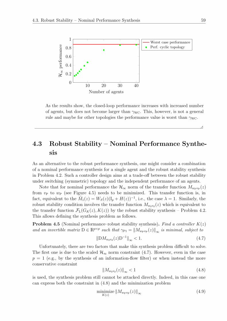
4.3. Robust Stability – Nominal Performance Synthesis 59
10 20 30 400
0.2
0.4
0.6
0.8
1
Number of agents
H∞
per
form
ance
Worst case performance
Perf. cyclic topology
As the results show, the closed-loop performance increases with increased number
of agents, but does not become larger than γWC. This, however, is not a general
rule and maybe for other topologies the performance value is worst than γWC.
4.3 Robust Stability – Nominal Performance Synthe-
sis
As an alternative to the robust performance synthesis, one might consider a combination
of a nominal performance synthesis for a single agent and the robust stability synthesis
in Problem 4.2. Such a controller design aims at a trade-off between the robust stability
under switching (symmetric) topology and the independent performance of an agents.
Note that for nominal performance the H∞ norm of the transfer function MwPvP(z)
from vP to wP (see Figure 4.5) needs to be minimized. This transfer function is, in
fact, equivalent to the M1(z) = WS(z)(Ip + H(z))−1, i.e., the case λ = 1. Similarly, the
robust stability condition involves the transfer function Mwδvδ(z) which is equivalent to
the transfer function FL(GK(z), K(z)) by the robust stability synthesis – Problem 4.2.
This allows defining the synthesis problem as follows.
Problem 4.5 (Nominal performance–robust stability synthesis). Find a controller K(z)
and an invertible matrix D ∈ Rp×p such that γP1 = ‖MwPvP(z)‖∞ is minimal, subject to
‖DMwδvδ(z)D−1‖∞ < 1. (4.7)
Unfortunately, there are two factors that make this synthesis problem difficult to solve.
The first one is due to the scaled H∞ norm constraint (4.7). However, even in the case
p = 1 (e.g., by the synthesis of an information-flow filter) or when instead the more
conservative constraint
‖Mwδvδ(z)‖∞ < 1 (4.8)
is used, the synthesis problem still cannot be attacked directly. Indeed, in this case one
can express both the constraint in (4.8) and the minimization problem
minimizeK(z)
‖MwPvP(z)‖∞ (4.9)
60 Chapter 4. Controller and Filter Synthesis Techniques
as LMIs and solve them independently. The necessary LMI conditions can be derived from
the inequality in (3.15), e.g., using a linearization change of variables (see, e.g., [Scherer
et al., 1997]) and the obtained controllers will be of the same order as the order of the
corresponding generalized plant. However, the above synthesis problem requires solving
both LMIs simultaneously with the same controller. This causes a problem, since Mwδvδ(z)
and MwPvP(z) are of different orders. Indeed the former transfer function is of the same
order as P (z), whereas the latter is of order equal the order of P (z) plus the orders of all
shaping filters.
The difference in the orders of the transfer functions can be avoided if static shaping
filters are used, but as the desired performance constraints are frequency dependent, such
static gains can rarely achieve satisfactory results. An alternative approach, using a direct
optimization method and based on a concept of simultaneous stabilization, i.e., a single
controller stabilizing multiple plants, will be exploited in Section 5.3.
4.4 Nominal Performance Synthesis
If for a vehicle formation the topology and the communication delays are known and
fixed, one might want to synthesize a nominal controller for that MAS, that is a controller
achieving the best possible closed-loop performance. Indeed, considering the topology as
uncertain and applying any of the introduced above synthesis techniques will result in a
conservative result (see Section 3.4). On the other hand, none of the controller synthesis
techniques reviewed in Section 2.3.1 is designed for a nominal controller/filter synthesis
for a given topology. The closest approach to a nominal synthesis is the decomposition
approach in [Massioni and Verhaegen, 2009] when applied to an undirected topology
without communication-delays, as then the LMIs corresponding to the smallest (i.e.,
λ1 = 0) and largest (λN) eigenvalues of L need to be considered. However, even a
controller designed by this approach will be conservative, as in fact it will guarantee the
robust performance for all decomposed systems with λi ∈ [0, λN ], rather than for the
particular set of eigenvalues corresponding to L.
An alternative approach is to consider directly the performance of the closed-loop
system in Figure 4.4(a) and search for a controller K(z), such that when replicated to
each agent γNP = ‖Mwv(z)‖∞ is minimal.
In order to simplify the following diagrams, assume that K(z) =[Kf(z) Kl(z)
],
that the local feedback (over φi) is closed and that it results in a transfer function
P (z) = FL(P (z), Kl(z)). Then, the transfer function of an agent can be written as
H(z) = P (z)Kf(z). The design process can be applied also for synthesis of K(z) directly,
but then one should take care that the inputs and outputs of the generalized plant are
accordingly arranged.
Now, one can equivalently represent the closed-loop as shown in Figure 4.6. Note
that although the plant P(z) = IN ⊗ P (z) and the filter WS(z) = IN ⊗WS(z) are both
with replicated structure, the generalized plant is not. This is due to the presence of the
Laplacian matrix L (or transfer function L(z) when communication delays are present).
As in what follows the closed-loop performance from v to w is addressed directly, one is
not restricted to performance filters with replicated structure and could apply any shaping
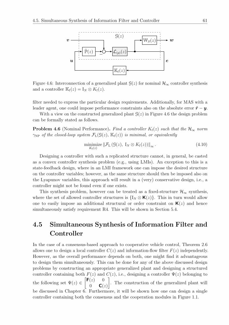
4.5. Simultaneous Synthesis of Information Filter and Controller 61
WS(z)
P(z) L(p)(z)
Kf(z)
wv
−eu
G(z)
Figure 4.6: Interconnection of a generalized plant G(z) for nominal H∞ controller synthesis
and a controller Kf(z) = IN ⊗Kf(z).
filter needed to express the particular design requirements. Additionally, for MAS with a
leader agent, one could impose performance constraints also on the absolute error r − y.
With a view on the constructed generalized plant G(z) in Figure 4.6 the design problem
can be formally stated as follows.
Problem 4.6 (Nominal Performance). Find a controller Kf(z) such that the H∞ norm
γNP of the closed-loop system FL(G(z), Kf(z)) is minimal, or equivalently
minimizeKf(z)
‖FL (G(z), IN ⊗Kf(z))‖∞ . (4.10)
Designing a controller with such a replicated structure cannot, in general, be casted
as a convex controller synthesis problem (e.g., using LMIs). An exception to this is a
state-feedback design, where in an LMI framework one can impose the desired structure
on the controller variables; however, as the same structure should then be imposed also on
the Lyapunov variables, this approach will result in a (very) conservative design, i.e., a
controller might not be found even if one exists.
This synthesis problem, however can be treated as a fixed-structure H∞ synthesis,
where the set of allowed controller structures is {IN ⊗ K(z)}. This in turn would allow
one to easily impose an additional structural or order constraint on K(z) and hence
simultaneously satisfy requirement R4. This will be shown in Section 5.4.
4.5 Simultaneous Synthesis of Information Filter and
Controller
In the case of a consensus-based approach to cooperative vehicle control, Theorem 2.6
allows one to design a local controller C(z) and information-flow filter F (z) independently.
However, as the overall performance depends on both, one might find it advantageous
to design them simultaneously. This can be done for any of the above discussed design
problems by constructing an appropriate generalized plant and designing a structured
controller containing both F (z) and C(z), i.e., designing a controller Ψ(z) belonging to
the following set Ψ(z) ∈[
F(z) 0
0 C(z)
]. The construction of the generalized plant will
be discussed in Chapter 6. Furthermore, it will be shown how one can design a single
controller containing both the consensus and the cooperation modules in Figure 1.1.
62 Chapter 4. Controller and Filter Synthesis Techniques
Just as the requirement for simple controllers, the robust performance design, the
nominal performance–robust stability design and the nominal performance design, this
approach to simultaneous synthesis of filter and controller leads to the problem of designing
a controller with structural constraints. This problem is addressed in the following chapter.
Publications
The non-scaled version of Problem 4.4 has been presented in [Popov and Werner, 2009]
and a scaled version in [Pilz et al., 2009], where also the construction of the corresponding
generalized plant has been detailed. The nominal controller synthesis in Problem 4.6 has
been discussed in [Popov and Werner, 2010].
Chapter 5
Fixed-Structure Controller Synthesis
Simplicity is the ultimate sophistication.
Leonardo da Vinci
In the previous chapter it was demonstrated, that the problem of a distributed controller
synthesis for a multi-agent system can be expressed in the H∞ framework, as it allows
incorporating both requirements on the stability as well as on the performance of the MAS.
Fortunately, although the posed problems could not be solved directly, each of them could
be reformulated as a design of a controller with structural restrictions. Additionally, as
discussed in the Introduction, agents in a multi-agent system often posses limited energy
supply, are equipped with a limited processing power or only a limited portion of the
available processing time is allocated to the control algorithm. These restrictions, impose
the additional requirement for a low-order and efficient controller, such as P, PI and PID.
Moreover, simple controllers are preferred since they can be easily implemented, validated
and if needed re-tuned. In the following, the term fixed-structure controller will be
used to denote both a controller with order restriction (e.g., static feedback gain (P), 1st,
2nd, etc., order controller) as well as with structural restriction (e.g., strictly proper, PI,
PID, repeated coefficients, etc.). This chapter addresses the fixed-structure H∞ controller
synthesis problem and shows how the design problems formulated in the previous chapter
can be solved.
Consider a standard (i.e., non-scaled) H∞ synthesis problem and the interconnection in
Figure 5.1, where G(z) is a generalized plant incorporating appropriate shaping filters and
scalings representing the control requirements, and K(z) is the controller (representing
either a local controller C(z), an information-filter F (z) or a formation controller K(z)
- see Section 2.3). Then, the fixed-structure H∞ controller synthesis problem can be
formally defined as follows.
Problem 5.1 (Fixed-structure H∞ synthesis). Find a controller K(z), belonging to the
set K(z) of controllers with the desired structure, such that the H∞ norm of closed-loop
transfer function M(z) = FL(G(z), K(z)) from v to w is minimal, or equivalently
minimizeK(z)∈K(z)
‖FL (G(z), K(z))‖∞. (5.1)
63
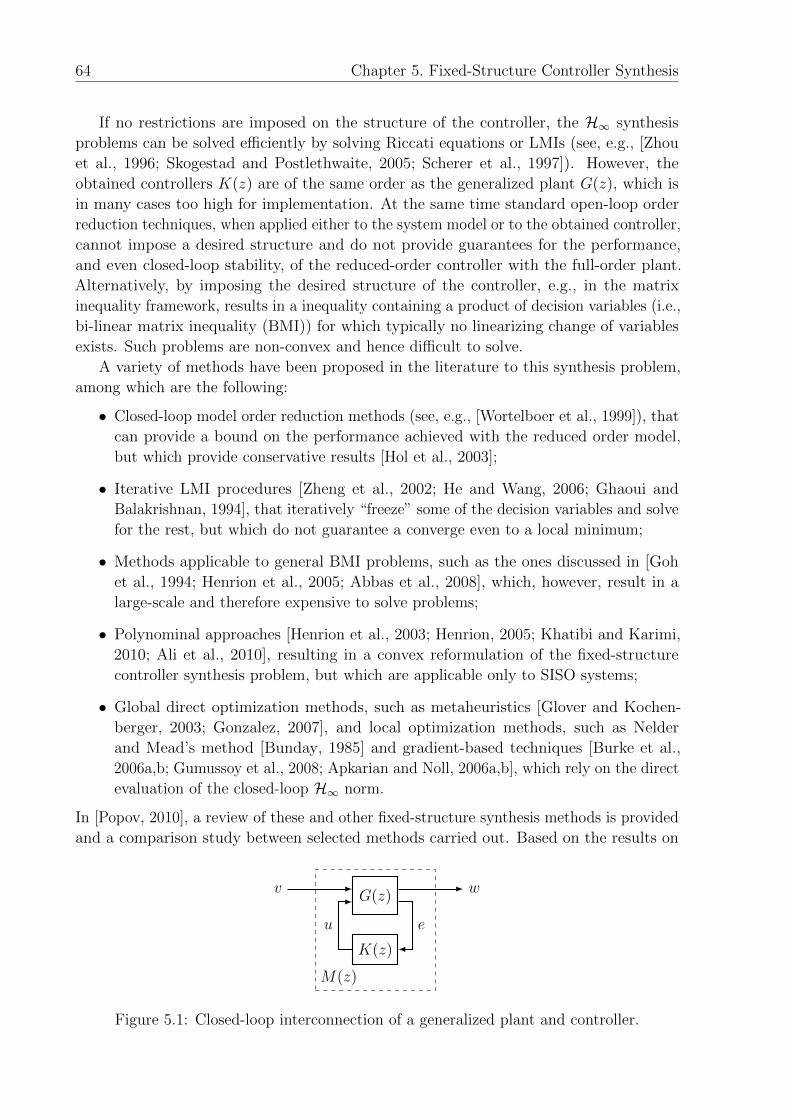
64 Chapter 5. Fixed-Structure Controller Synthesis
If no restrictions are imposed on the structure of the controller, the H∞ synthesis
problems can be solved efficiently by solving Riccati equations or LMIs (see, e.g., [Zhou
et al., 1996; Skogestad and Postlethwaite, 2005; Scherer et al., 1997]). However, the
obtained controllers K(z) are of the same order as the generalized plant G(z), which is
in many cases too high for implementation. At the same time standard open-loop order
reduction techniques, when applied either to the system model or to the obtained controller,
cannot impose a desired structure and do not provide guarantees for the performance,
and even closed-loop stability, of the reduced-order controller with the full-order plant.
Alternatively, by imposing the desired structure of the controller, e.g., in the matrix
inequality framework, results in a inequality containing a product of decision variables (i.e.,
bi-linear matrix inequality (BMI)) for which typically no linearizing change of variables
exists. Such problems are non-convex and hence difficult to solve.
A variety of methods have been proposed in the literature to this synthesis problem,
among which are the following:
• Closed-loop model order reduction methods (see, e.g., [Wortelboer et al., 1999]), that
can provide a bound on the performance achieved with the reduced order model,
but which provide conservative results [Hol et al., 2003];
• Iterative LMI procedures [Zheng et al., 2002; He and Wang, 2006; Ghaoui and
Balakrishnan, 1994], that iteratively “freeze” some of the decision variables and solve
for the rest, but which do not guarantee a converge even to a local minimum;
• Methods applicable to general BMI problems, such as the ones discussed in [Goh
et al., 1994; Henrion et al., 2005; Abbas et al., 2008], which, however, result in a
large-scale and therefore expensive to solve problems;
• Polynominal approaches [Henrion et al., 2003; Henrion, 2005; Khatibi and Karimi,
2010; Ali et al., 2010], resulting in a convex reformulation of the fixed-structure
controller synthesis problem, but which are applicable only to SISO systems;
• Global direct optimization methods, such as metaheuristics [Glover and Kochen-
berger, 2003; Gonzalez, 2007], and local optimization methods, such as Nelder
and Mead’s method [Bunday, 1985] and gradient-based techniques [Burke et al.,
2006a,b; Gumussoy et al., 2008; Apkarian and Noll, 2006a,b], which rely on the direct
evaluation of the closed-loop H∞ norm.
In [Popov, 2010], a review of these and other fixed-structure synthesis methods is provided
and a comparison study between selected methods carried out. Based on the results on
G(z)
K(z)
wv
eu
M(z)
Figure 5.1: Closed-loop interconnection of a generalized plant and controller.
65
a set of over 100 continuous-time benchmark problems, the gradient-based techniques
proposed in [Burke et al., 2006a] and [Apkarian and Noll, 2006b] are identified as the most
promising fixed-structured H∞ synthesis techniques (in terms of achieved closed-loop H∞norm and computational load). The former one is freely available as a toolbox for Matlab –
hifoo. Additionally, a study of the performance of hifoo on a set of benchmark problems
can be found in [Gumussoy and Overton, 2008; Gumussoy et al., 2008, 2009].
The difference between the two gradient-based techniques stems from the different
approaches they use to handle discontinuities due to non-smoothness in the objective
space. Let x ∈ Rn denote the vector of controller coefficients, i.e., the decision variables,
and let f(x) : Rn → R denote the function computing the closed-loop H∞ norm with that
controller. Then, because the structure of the controller is restricted, f(x) might not be
differentiable at every x and hence no (unique) gradient could be computed. The two
techniques deal with this problem as follows.
• The approach of [Burke et al., 2006a] adds a small perturbation ε ∈ Rn to x and
then computes the gradient. Moreover, as a last optimization stage, this approach
uses a gradient-sampling technique by which the gradients in x+ εh are computed for
several, small, randomly selected εh, and a stabilizing descent direction is calculated.
• The method proposed in [Apkarian and Noll, 2006b] uses a subgradient approach, by
which in a point x where f(x) is non-smooth, not a single gradient but rather a set
of gradients is considered, and the steepest descent direction computed. The relation
between the gradient and the subgradient of a function is outlined in Appendix C.3.
However, since both gradient-based techniques are developed for continuous-time H∞synthesis, they cannot be directly applied to discrete-time ones. An often used approach
is to convert the discrete-time generalized plant to a continuous-time one via a bilinear
(Tustin) transformation, perform a continuous-time controller synthesis and then transform
the controller to a discrete-time using the inverse bilinear transformation. However, as
this might cause problems due to frequency warping [Astrom and Wittenmark, 1997] and
since the structural restrictions might not be preserved during the transformation, in the
following the gradient calculations are modified, so that the synthesis can be performed
directly in discrete-time domain.
The remainder of this chapter is structured as follows. In Section 5.1 the necessary
gradient calculations for a fixed-structure discrete-time H∞ synthesis are presented. These
results are then used in Section 5.2 to obtain a gradient with respect to the scaling matrix
D in a scaled H∞ synthesis problem, needed for solving Problems 4.4 and 4.5. The latter
problem is addressed in more detail in Section 5.3. Finally, in Section 5.4 the problem of
designing an H∞ controller with replicated sub-blocks will be addressed, i.e., the necessary
gradient computations for solving the nominal H∞ performance in Problem 4.6 will be
presented.
It should be mentioned that this chapter is of an independent interest since the problem
of designing controllers with restricted structure appears not only in the field of multi-agent
systems, but also in control law synthesis for a single system, when limited processing
capabilities are available or a simple controller is required. Moreover, the simultaneous
optimization over controller and scaling, presented in Section 5.2, is applicable not only to
66 Chapter 5. Fixed-Structure Controller Synthesis
the robust stability design for a MAS, but to any H∞ controller synthesis problem where
structured uncertainty is present or when robust performance needs to be guaranteed.
Finally, besides for distributed control problem for a MAS, the results in Section 5.4 can
be of an interest for other control applications where the plant has a replicated structure
or a controller with replicated sub-blocks needs to be imposed.
In the following, it will be assumed that M(z) = FL(G(z), K(z)) is stable, has a
minimal state-space model
M(z) =
A B
C D
,and that the closed-loop H∞ norm f = ‖M(z)‖∞ is attained at frequency ωx, i.e.,
f = ‖M(z)‖∞ = σ(M(ejωx)
)= σ(Mx), (5.2)
where
Mx = C(ejωxIn − A)−1B +D, (5.3)
and n is the number of states of M(z) (i.e., A ∈ Rn×n).
As the following sections deal with gradient of matrices, for the purpose of following
the proofs, one might find it useful to accustom oneself with the basics of matrix calculus,
summarized in Appendix B, before proceeding further.
5.1 Discrete-time H∞ Synthesis
The previously discussed restrictions in the controller structure/order are often accompanied
by a limited sampling frequency, but demanding performance requirements. Furthermore,
often a discrete-time plant model is available, for example obtained via black-box identifi-
cation. As already discussed, a controller for such a system can be designed by converting
the system model to continuous-time, performing a continuous-time controller synthesis
and discretizing the obtained controller. However, such synthesis might be misleading
since potential problems like frequency warping [Astrom and Wittenmark, 1997] are not
considered or it might not be possible to impose structure restrictions on the controller,
such as properness. In the following, the necessary modifications to the gradient-based
technique are discussed.
Consider the fixed-structure H∞ synthesis problem in (5.1). Since the H∞ norm is
defined only for stable systems, a controller K(z) should simultaneously stabilize the system
and minimize the closed-loop H∞ norm. This is implicitly taken care of when using LMIs,
since the existence of a Lyapunov matrix satisfying the LMI conditions guarantees the
closed-loop stability. However, this is not the case when using gradient-based methods and
hence the design process is split into two steps – stabilization and H∞ norm minimization.
These are the very same two stages employed in hifoo [Burke et al., 2006a] and [Apkarian
and Noll, 2006b].
5.1. Discrete-time H∞ Synthesis 67
5.1.1 Search for a Stabilizing Controller
In the continuous-time approach taken in [Apkarian and Noll, 2006b], the first step – the
search for a stabilizing controller – is performed via a shifted H∞ -norm minimization.
A corresponding approach for discrete-time systems would be scaling of the closed-loop
system matrix. Here, however, a minimization of the spectral radius is proposed, as
it directly addresses the problem of finding a stabilizing controller. This initialization
procedure can then be applied also to the approach in [Apkarian and Noll, 2006a,b]. Hence,
here only the necessary changes to the approach used in [Burke et al., 2006a] are discussed.
Let A ∈ Rn×n denote the closed-loop system matrix obtained with a particular controller
K(z). In the continuous-time case the stability of the closed-loop is equivalent to the
condition α (A) < 1, where α (A) denotes the spectral abscissa of A, i.e., the maximal
real part of the closed-loop eigenvalues. The corresponding condition in the discrete-time
case is ρ (A) < 1, where ρ (A) is the spectral radius of A, i.e., the closed-loop eigenvalue
with maximal magnitude. Since the gradient computation of α (A) and the required chain
rule calculations leading to the dependence on K(z) are discussed in [Burke et al., 2003;
Millstone, 2006], in the following only the necessary gradient of ρ (A) w.r.t. A is provided.
In what follows, the dependence on A is omitted when clear from the context.
Theorem 5.1. Let λi = λi(A) ∈ spec(A) be the eigenvalues of the closed-loop system
matrix A ∈ Rn×n, i = 1, . . . , n. Let λh be an eigenvalue at which ρ (A) is attained, i.e.,
ρ (A) = maxi |λi| = |λh|. Assume further that λh is with algebraic multiplicity one (which
allows for complex conjugated pole pairs). Then the matrix gradient of ρ w.r.t. A is
∇Aρ = Re
{λh|λh|
yx∗T
y∗Tx
}. (5.4)
Proof. In order to obtain the needed gradient of ρ (A) w.r.t. the elements of A (and later
w.r.t. the design coefficients of K(z)), one needs to obtain the gradient |λh| w.r.t. A.
First, note that
ρ (A) = |λh| =√λ∗hλh.
Then the partial derivatives of ρ w.r.t. λh and λ∗h are (see Appendix B.2.2)
∇λhρ =∂ρ
∂λh=
1
2
λ∗h√λ∗hλh
=1
2
λ∗h|λh|
; ∇λ∗hρ =∂ρ
∂λ∗h=
1
2
λh√λ∗hλh
=1
2
λh|λh|
,
where it is used that for a complex number q
∂q
∂q∗=∂q∗
∂q= 0.
The chain rule for real-valued function (such as the spectral radius) of a complex variable
reads (see Appendix B.2.2)
∂ρ
∂Aik=
∂ρ
∂λh
∂λh∂Aik
+∂ρ
∂λ∗h
∂λ∗h∂Aik
=∂ρ
∂λh
∂λh∂Aik
+
(∂ρ
∂λh
)∗∂λ∗h∂Aik
. (5.5)
For a small number θ and a matrix A(θ) = A0 +Pθ, a result from eigenvalue perturbation
theory [Horn and Johnson, 1985; Meyer, 2000] states, that if λh is an eigenvalue of A(0)
68 Chapter 5. Fixed-Structure Controller Synthesis
with corresponding right and left eigenvectors x and y, then
dλh(A)
dθ=y∗T dA(θ)
dθx
y∗Tx.
From this it follows that∂λh∂Aik
=y∗TEikx
y∗Tx,
where Eik = eieTk is an elementary matrix, with ei and ek being columns i and k of In.
As x∗ and y∗ are the right and left eigenvectors corresponding to λ∗h it follows that
∂λ∗h∂Aik
=yTEikx
∗
yTx∗.
Substituting in (5.5) obtains
∂ρ
∂Aik=
1
2
λ∗h|λh|
y∗TEikx
y∗Tx+
1
2
λh|λh|
yTEikx∗
yTx∗,
which is a sum of a complex number and its conjugate and hence
∂ρ
∂Aik=Re
{λ∗h|λh|
y∗TEikx
y∗Tx
}(5.6)
=Re {〈2∇λhρ ∗, ∇Aikλh 〉} = Re{⟨
2∇λ∗hρ , ∇Aikλh⟩}, (5.7)
which is consistent with the result in [Brandwood, 1983, Eq. (15)].
Finally, applying the chain rule for the product of complex matrices (B.9) to (5.6)
leads to the desired gradient of ρ (A) w.r.t. A in (5.4). �
An alternative proof, based on expressing λh via a two element vector variable[Re {λh} Im {λh}
], is presented in [Han et al., 2003; Popov et al., 2010b].
Remark 5.1. If the λh is of higher algebraic multiplicity than one, one should use the
perturbation approach as in [Burke et al., 2006a,b], i.e., use the eigenvalues and eigenvectors
of A+ δA instead, where δA ∈ Rn×n is randomly selected matrix, such that ‖δA‖ is much
smaller than ‖A‖. The subgradient approach in [Apkarian and Noll, 2006b] can be applied
only to the case when the system matrix A is Hermitian A = A∗T, but not to a general
matrix, as the search for a descent direction cannot be conveniently expressed as an
optimization problem.
5.1.2 Minimizing the Closed-Loop H∞ Norm
Since during the second step – the minimization of ‖M(z)‖∞ – the gradient-based tech-
niques rely on the computation of the H∞ norm by external functions (e.g. the norm
function in matlab), the only change required is to account for the frequency range of
interest, i.e., ω ∈ [0, π] rather than ω ∈ [0, ∞]. Assuming that the H∞ norm is attained
at frequency ωx, one could compute the gain of the closed-loop system as
Mx = B(ejωxIn − A)−1C +D.
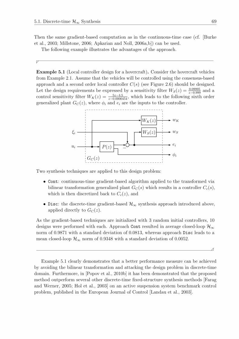
5.1. Discrete-time H∞ Synthesis 69
Then the same gradient-based computation as in the continuous-time case (cf. [Burke
et al., 2003; Millstone, 2006; Apkarian and Noll, 2006a,b]) can be used.
The following example illustrates the advantages of the approach.
Example 5.1 (Local controller design for a hovercraft). Consider the hovercraft vehicles
from Example 2.1. Assume that the vehicles will be controlled using the consensus-based
approach and a second order local controller C(s) (see Figure 2.6) should be designed.
Let the design requirements be expressed by a sensitivity filter WS(z) = 0.09995z−0.999
and a
control sensitivity filter WK(z) = 5z−4.5z−0.0000454
, which leads to the following sixth order
generalized plant GC(z), where φi and ei are the inputs to the controller.
WK(z)
WS(z)
P (z) −
ξi
wK
wS
ei
φi
ui
GC(z)
Two synthesis techniques are applied to this design problem:
• Cont: continuous-time gradient-based algorithm applied to the transformed via
bilinear transformation generalized plant GC(s) which results in a controller Cc(s),
which is then discretized back to Cc(z), and
• Disc: the discrete-time gradient-based H∞ synthesis approach introduced above,
applied directly to GC(z).
As the gradient-based techniques are initialized with 3 random initial controllers, 10
designs were performed with each. Approach Cont resulted in average closed-loop H∞norm of 0.9871 with a standard deviation of 0.0813, whereas approach Disc leads to a
mean closed-loop H∞ norm of 0.9348 with a standard deviation of 0.0052.
Example 5.1 clearly demonstrates that a better performance measure can be achieved
by avoiding the bilinear transformation and attacking the design problem in discrete-time
domain. Furthermore, in [Popov et al., 2010b] it has been demonstrated that the proposed
method outperform several other discrete-time fixed-structure synthesis methods [Farag
and Werner, 2005; Hol et al., 2003] on an active suspension system benchmark control
problem, published in the European Journal of Control [Landau et al., 2003].
70 Chapter 5. Fixed-Structure Controller Synthesis
5.2 Simultaneous Search over Controller and Scal-
ings
In Section 4.2 it was shown, that the robust performance synthesis problem results in a
scaled H∞ synthesis, i.e.,
minimizeK(z)
D∈Rp×ps.t. ∃D−1
∥∥∥∥[D 0
0 Inw
]FL(G(z), K(z))
[D−1 0
0 Inv
]∥∥∥∥∞,
which contains a product of scaling and controller variables and cannot be solved as a
convex problem. A typical approach is to use an iterative procedure, such as D-K synthesis
[Zhou et al., 1996; Balas et al., 2001] or S-K synthesis [Apkairan and Adams, 2000], by
which at each step either the controller or the scaling variables are fixed and it is solved
for the others. However, as the problem is not jointly-convex in both variables, such
techniques do not even guarantee to converge to a local minimum.
In this section, it will be demonstrated how the above problem can be solved using the
gradient-based H∞ synthesis methods by appropriately calculating the gradient w.r.t. the
scaling matrices and the controller. In addition, it will be shown how the gradients can be
modified to allow for dynamic scalings D(z). This latter case is of interest for designing
robust controllers satisfying Theorem 3.2, since then the difficult to solve structured
singular value problem is exchanged with its upper boundary and hence results in a
dynamically-scaled H∞ problem. Additionally, this problem occurs when parametric
uncertainty is present, as well as when robust performance synthesis needs to be performed
(i.e., when inputs and outputs both used for performance evaluation and connected to
uncertain gains are present).
5.2.1 Static Scalings
Let M(z) = FL(G(z), K(z)) and
Q(z) =
[D 0
0 Inw
]M(z)
[D−1 0
0 Inv
].
Moreover, let the matrices of M(z) be appropriately partitioned as
M(z) =
AM BM
CM DM
=
AM B1 B2
C1 D11 D12
C2 D21 D22
,so that for Q(z) one obtains
Q(z) =
AM B1D B2
D−1C1 D−1D11D D−1D12
C2 D21D D22
=
AQ BQ,1 BQ,2
CQ,1 DQ,11 DQ,12
CQ,2 DQ,21 DQ,22
. (5.8)
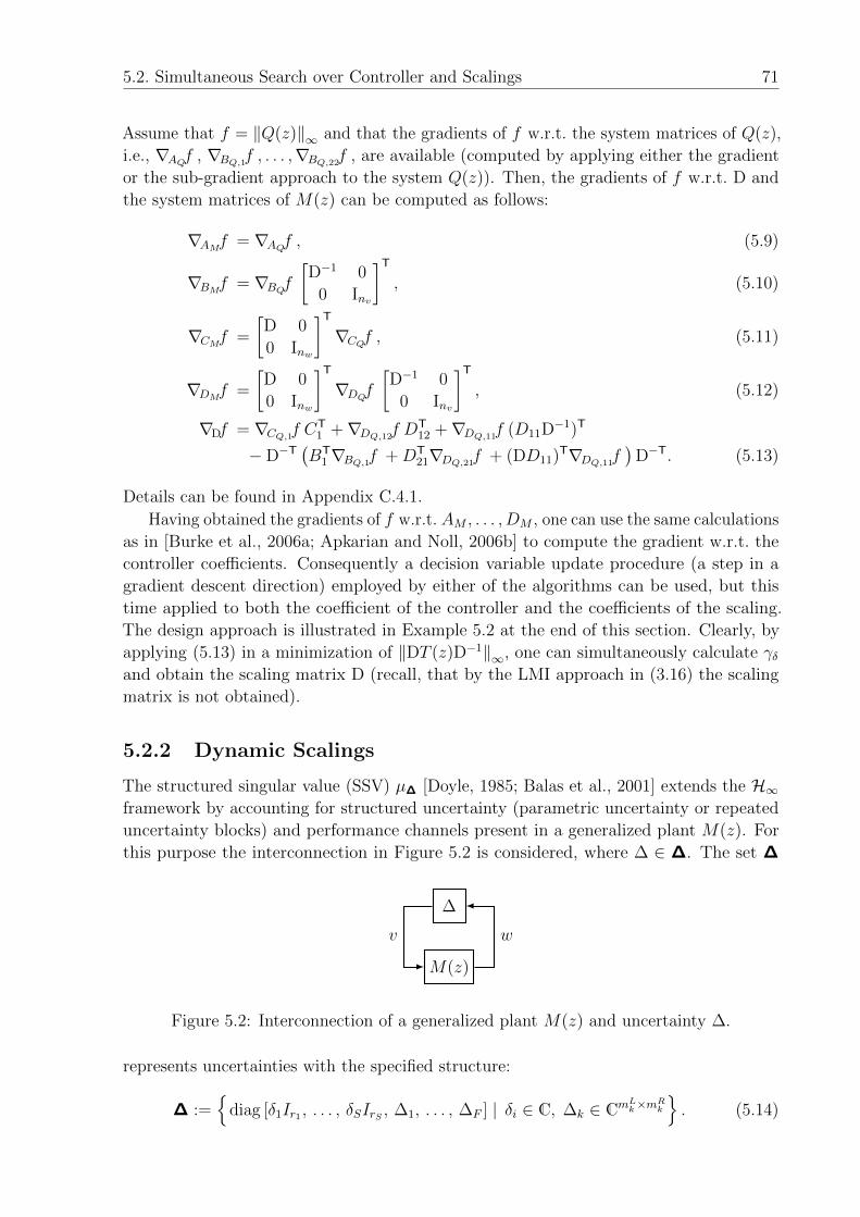
5.2. Simultaneous Search over Controller and Scalings 71
Assume that f = ‖Q(z)‖∞ and that the gradients of f w.r.t. the system matrices of Q(z),
i.e., ∇AQf , ∇BQ,1f , . . . ,∇BQ,22f , are available (computed by applying either the gradient
or the sub-gradient approach to the system Q(z)). Then, the gradients of f w.r.t. D and
the system matrices of M(z) can be computed as follows:
∇AMf = ∇AQf , (5.9)
∇BMf = ∇BQf[D−1 0
0 Inv
]T, (5.10)
∇CMf =
[D 0
0 Inw
]T∇CQf , (5.11)
∇DMf =
[D 0
0 Inw
]T∇DQf
[D−1 0
0 Inv
]T, (5.12)
∇Df = ∇CQ,1f CT1 +∇DQ,12f DT
12 +∇DQ,11f (D11D−1)T
−D−T(BT
1∇BQ,1f +DT21∇DQ,21f + (DD11)T∇DQ,11f
)D−T. (5.13)
Details can be found in Appendix C.4.1.
Having obtained the gradients of f w.r.t. AM , . . . , DM , one can use the same calculations
as in [Burke et al., 2006a; Apkarian and Noll, 2006b] to compute the gradient w.r.t. the
controller coefficients. Consequently a decision variable update procedure (a step in a
gradient descent direction) employed by either of the algorithms can be used, but this
time applied to both the coefficient of the controller and the coefficients of the scaling.
The design approach is illustrated in Example 5.2 at the end of this section. Clearly, by
applying (5.13) in a minimization of ‖DT (z)D−1‖∞, one can simultaneously calculate γδand obtain the scaling matrix D (recall, that by the LMI approach in (3.16) the scaling
matrix is not obtained).
5.2.2 Dynamic Scalings
The structured singular value (SSV) µ∆ [Doyle, 1985; Balas et al., 2001] extends the H∞framework by accounting for structured uncertainty (parametric uncertainty or repeated
uncertainty blocks) and performance channels present in a generalized plant M(z). For
this purpose the interconnection in Figure 5.2 is considered, where ∆ ∈ ∆. The set ∆
∆
v w
M(z)
Figure 5.2: Interconnection of a generalized plant M(z) and uncertainty ∆.
represents uncertainties with the specified structure:
∆ :={
diag [δ1Ir1 , . . . , δSIrS , ∆1, . . . , ∆F ] | δi ∈ C, ∆k ∈ CmLk×m
Rk
}. (5.14)
72 Chapter 5. Fixed-Structure Controller Synthesis
The total dimension of the uncertainty block should match the dimension of v and w, i.e.,
∆ ∈ Cnv×nw , or alternatively
S∑i=1
ri +F∑k=1
mLk = nv,
S∑i=1
ri +F∑k=1
mRk = nw.
It is furthermore assumed that ∆ is normalized, i.e., each ∆ ∈ ∆ satisfies
σ(∆) ≤ 1. This can be achieved by introducing appropriate scalings in the input and
output matrices of M(z).
The definition of the structured singular value µ∆ is provided in Appendix D and its
properties can be found in, e.g., [Packard and Doyle, 1993; Balas et al., 2001; Dailey,
1991]. Unfortunately the computation of µ∆ is by itself an NP-hard problem [Braatz et al.,
1994]. Hence, often instead of µ∆(M(z)) an upper bound, depending on additional scaling
variables, is used. Define the sets of invertible matrices DL and DR commuting with ∆ as
DL :={
diag[D1, . . . , DS, d1ImL1 , . . . , dF ImLF
] ∣∣∣ Di ∈ Cri×ri , dk ∈ R}, (5.15)
DR :={
diag[D1, . . . , DS, d1ImR1 , . . . , dF ImRF
] ∣∣∣ Di ∈ Cri×ri , dk ∈ R}, (5.16)
where i = 1, . . . , S and k = 1, . . . , F .
As the coefficients of both DL and DR scalings are identical they will be referred to as D
scaling and the set of allowed scalings as D. The commuting and invertability requirements
allow to write DL∆ = ∆DR and
DR∆D−1L = ∆, ∀D ∈ D, ∀∆ ∈ ∆.
Note that the requirement DL being invertible is equivalent to the more often met
requirements Di = D∗Ti , dk > 0 (cf. [Packard and Doyle, 1993]). The following are
well-known properties of µ∆ for a matrix M :
• µ∆(DRMD−1L ) = µ∆(M), ∀D ∈ D,
• µ∆(M) ≤ σ(M),
• µ∆(M) ≤ infD∈D
σ(DRMD−1L ).
In a similar manner the results are extended to dynamic systems, in which case the
minimization of µ∆(M(z)) is exchanged with the minimization of the upper bound:
‖DR(z)M(z)D−1L (z)‖∞.
Now consider the generalized plant G(z) and a controller K(z) interconnected as shown
in Figure 5.3, where M(z) = FL(G(z), K(z)).
Let Q(z) = DR(z)M(z) D−1L (z). In order to apply a gradient-based algorithm to the
minimization of f = ‖Q(z)‖∞, the gradients of f w.r.t. the controller and the scalings are
necessary. Let
M(z) =
AM BM
CM DM
, DR(z) =
AR BR
CR DR
, DL(z) =
AL BL
CL DL
.
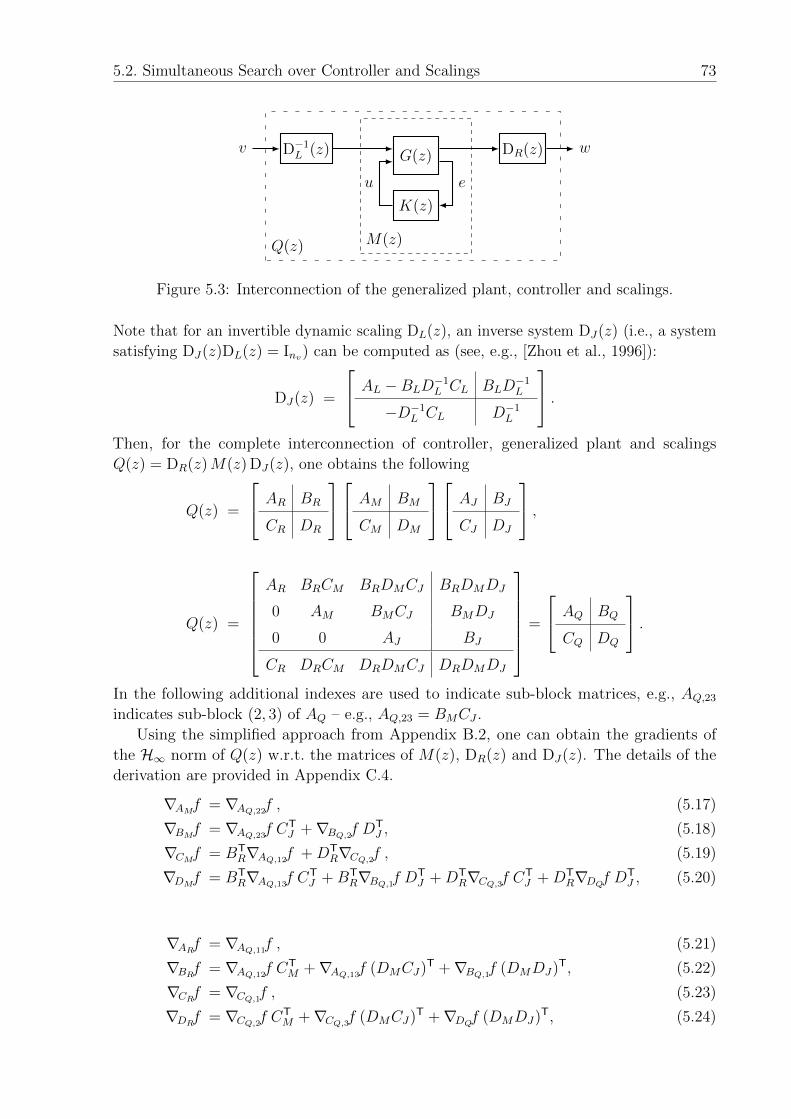
5.2. Simultaneous Search over Controller and Scalings 73
G(z)
K(z)
M(z)
D−1L (z) DR(z)v w
u e
Q(z)
Figure 5.3: Interconnection of the generalized plant, controller and scalings.
Note that for an invertible dynamic scaling DL(z), an inverse system DJ(z) (i.e., a system
satisfying DJ(z)DL(z) = Inv) can be computed as (see, e.g., [Zhou et al., 1996]):
DJ(z) =
AL −BLD−1L CL BLD
−1L
−D−1L CL D−1
L
.Then, for the complete interconnection of controller, generalized plant and scalings
Q(z) = DR(z)M(z) DJ(z), one obtains the following
Q(z) =
AR BR
CR DR
AM BM
CM DM
AJ BJ
CJ DJ
,
Q(z) =
AR BRCM BRDMCJ BRDMDJ
0 AM BMCJ BMDJ
0 0 AJ BJ
CR DRCM DRDMCJ DRDMDJ
=
AQ BQ
CQ DQ
.In the following additional indexes are used to indicate sub-block matrices, e.g., AQ,23
indicates sub-block (2, 3) of AQ – e.g., AQ,23 = BMCJ .
Using the simplified approach from Appendix B.2, one can obtain the gradients of
the H∞ norm of Q(z) w.r.t. the matrices of M(z), DR(z) and DJ(z). The details of the
derivation are provided in Appendix C.4.
∇AMf = ∇AQ,22f , (5.17)
∇BMf = ∇AQ,23f CTJ +∇BQ,2f DT
J , (5.18)
∇CMf = BTR∇AQ,12f +DT
R∇CQ,2f , (5.19)
∇DMf = BTR∇AQ,13f CT
J +BTR∇BQ,1f DT
J +DTR∇CQ,3f CT
J +DTR∇DQf DT
J , (5.20)
∇ARf = ∇AQ,11f , (5.21)
∇BRf = ∇AQ,12f CTM +∇AQ,13f (DMCJ)T +∇BQ,1f (DMDJ)T, (5.22)
∇CRf = ∇CQ,1f , (5.23)
∇DRf = ∇CQ,2f CTM +∇CQ,3f (DMCJ)T +∇DQf (DMDJ)T, (5.24)
74 Chapter 5. Fixed-Structure Controller Synthesis
∇AJf = ∇AQ,33f , (5.25)
∇BJf = ∇BQ,3f , (5.26)
∇CJf = (BRDM)T∇AQ,13f +BTM∇AQ,23f + (DRDM)T∇CQ,3f , (5.27)
∇DJf = (BRDM)T∇BQ,1f +BTM∇BQ,2f + (DRDM)T∇DQf . (5.28)
Then, using the matrix inversion rule (see Appendix C.1), one can obtain the gradient of
‖Q(z)‖∞ w.r.t. DL(z):
∇ALf =∇AJf , (5.29)
∇BLf = −∇AJf (D−1L CL)T +∇BJf (D−1
L )T, (5.30)
∇CLf = − (BLD−1L )T∇AJf − (D−1
L )T∇CJf , (5.31)
∇DLf = (BLD−1L )T∇AJf (D−1
L CL)T − (BLD−1L )T∇BJf (D−1
L )T
+ (D−1L )T∇CJf (D−1
L CL)T − (D−1L )T∇DJf (D−1
L )T. (5.32)
Finally, the corresponding coefficients from the matrices of DR(z) and DL(z) have to be
extracted and added up together to form the gradient w.r.t. a scaling factor D(z) – a
“virtual” scaling factor, containing only the necessary elements, i.e., the unique scaling
coefficients.
5.2.3 Replicated Structure Approach
An alternative approach to scaled H∞ synthesis has been recently proposed in [Apkarian,
2010]. The method expresses DL(z) = Inv + DL(z) and DR(z) = Inw + DR(z) and uses that
FL(Inv , −DL(z)) =(Inv + DL(z)
)−1= D−1
L (z).
This allows constructing a generalized plant G(z), such that the LFT interconnection
with K(z) = diag(K(z), DL(z), DR(z)
)is equivalent to Q(z), i.e., FL(G(z), K(z)) =
D−1L (z)M(z)DR(z). Because of the structure of DL and DR, the controller K(z) has
replicated sub-blocks: Di − Iri and dk − 1, i = 1, . . . , S, k = 1, . . . , F . As this results in a
design problem similar to the nominal performance synthesis problem (Section 4.4), the
needed gradient calculations will be discussed in Section 5.4.
Example 5.2 (Robust performance design of an information filter). Take up the
hovercraft vehicles from Example 2.1, assume that the local controller is designed as in
Example 5.1 and consider the problem of designing an information flow filter F (z) such
that the stability of a MAS under switching topology and time-varying communication
delays is guaranteed. Additionally, the filter should guarantee achieving information
consensus if the requirements on the topology discussed in [Chopra and Spong, 2006;
Wang and Elia, 2009b] or [Ren and Beard, 2005] are satisfied.
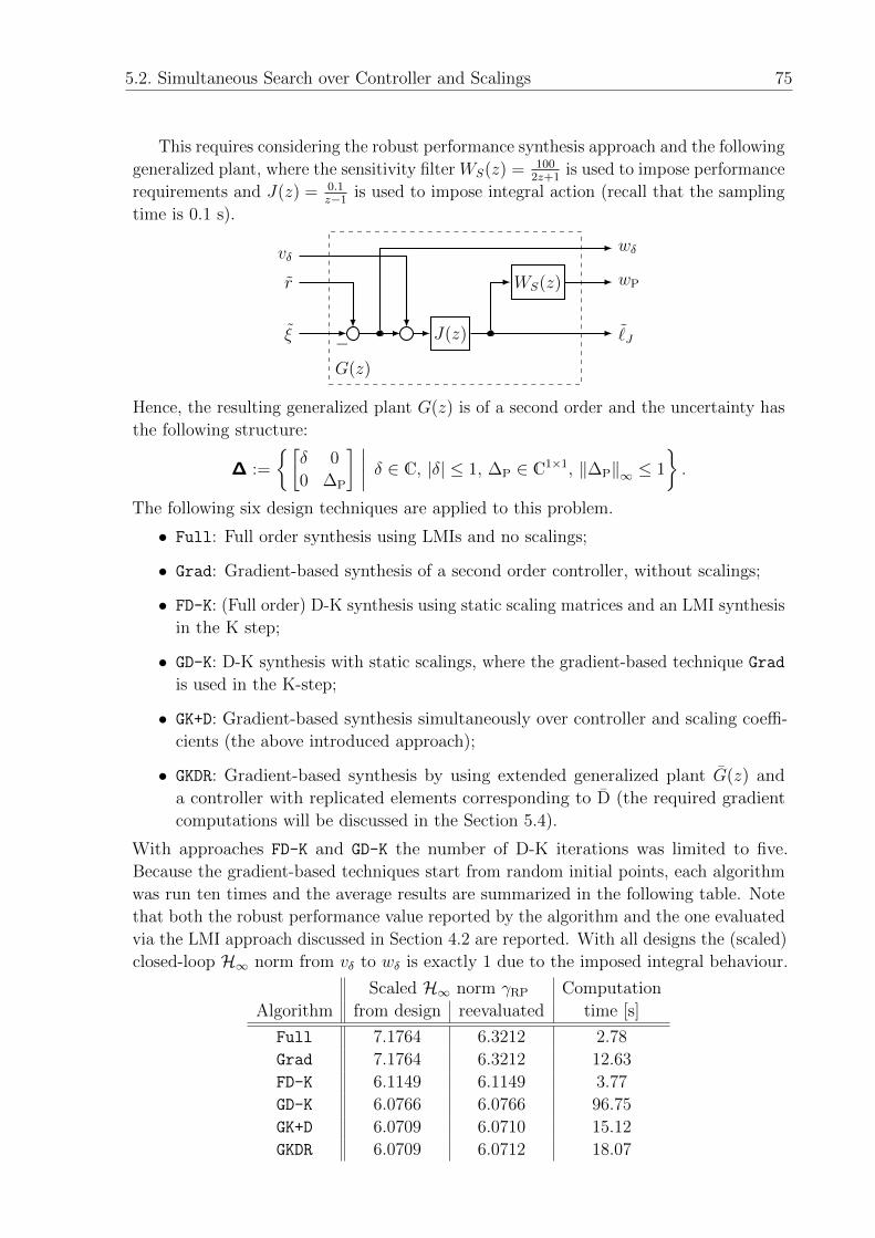
5.2. Simultaneous Search over Controller and Scalings 75
This requires considering the robust performance synthesis approach and the following
generalized plant, where the sensitivity filter WS(z) = 1002z+1
is used to impose performance
requirements and J(z) = 0.1z−1
is used to impose integral action (recall that the sampling
time is 0.1 s).
WS(z)
J(z)ξ − ˜J
r
vδwδ
wP
G(z)
Hence, the resulting generalized plant G(z) is of a second order and the uncertainty has
the following structure:
∆ :=
{[δ 0
0 ∆P
] ∣∣∣∣ δ ∈ C, |δ| ≤ 1, ∆P ∈ C1×1, ‖∆P‖∞ ≤ 1
}.
The following six design techniques are applied to this problem.
• Full: Full order synthesis using LMIs and no scalings;
• Grad: Gradient-based synthesis of a second order controller, without scalings;
• FD-K: (Full order) D-K synthesis using static scaling matrices and an LMI synthesis
in the K step;
• GD-K: D-K synthesis with static scalings, where the gradient-based technique Grad
is used in the K-step;
• GK+D: Gradient-based synthesis simultaneously over controller and scaling coeffi-
cients (the above introduced approach);
• GKDR: Gradient-based synthesis by using extended generalized plant G(z) and
a controller with replicated elements corresponding to D (the required gradient
computations will be discussed in the Section 5.4).
With approaches FD-K and GD-K the number of D-K iterations was limited to five.
Because the gradient-based techniques start from random initial points, each algorithm
was run ten times and the average results are summarized in the following table. Note
that both the robust performance value reported by the algorithm and the one evaluated
via the LMI approach discussed in Section 4.2 are reported. With all designs the (scaled)
closed-loop H∞ norm from vδ to wδ is exactly 1 due to the imposed integral behaviour.
Scaled H∞ norm γRP Computation
Algorithm from design reevaluated time [s]
Full 7.1764 6.3212 2.78
Grad 7.1764 6.3212 12.63
FD-K 6.1149 6.1149 3.77
GD-K 6.0766 6.0766 96.75
GK+D 6.0709 6.0710 15.12
GKDR 6.0709 6.0712 18.07
76 Chapter 5. Fixed-Structure Controller Synthesis
Several observations can be made based on the data in the above table. Firstly, by
comparing the results of Full and Grad it becomes apparent that the gradient-based
approach can obtain the same results in terms of closed-loop H∞ norm as the full-order
synthesis, but, naturally, at a higher computational cost. Secondly, the D-K iteration
scheme (techniques FD-K and GD-K) accounts for the structure of the uncertainty and
achieves better results than Full and Grad. Thirdly, and mainly – the simultaneous
optimization over both controller and scaling coefficients (i.e., techniques GK+D and GKDR)
achieves better results than the D-K iteration technique and with less computational
overhead. Indeed, the long computation times with GD-K is due to the fact that 5 D-K
iterations were performed and during each iteration a gradient-based search of the same
complexity as with Grad has been performed. The slight difference between the reported
scaled H∞ norm and the reevaluated one by GK+D and GDKR is due to the numeric
precision in solving the LMI problems by the reevaluation. The norm values, reported
by both algorithms, have been validated by evaluating the scaled H∞ norm with the
obtained scalings and information filter.
5.3 Simultaneous Stabilization
In [Gumussoy et al., 2008] a gradient-based approach to fixed-structure H∞ controller syn-
thesis is used to attack the problem of simultaneous stabilization of several
continuous-time generalized plants. A discrete-time equivalent will consider the gen-
eralized plants G0(z), G1(z), . . . , Gc(z), and the constraint optimization problem
minimizeK(z)∈K(z)
‖FL(G0(z), K(z))‖∞subject to ‖FL(Gk(z), K(z))‖∞ < %k, k = 1, . . . , nG
where %k ∈ R, %k > 0, k = 1, . . . , nG.
As the constraints cannot be directly imposed, in [Gumussoy et al., 2008] it is proposed
to attack the following optimization problem instead
minimizeK(z)∈K(z)
(‖FL(G0(z), K(z))‖∞ + β
c∑k=1
max (0, ‖FL(Gk(z), K(z))‖∞ − %k)),
where the value of β (much greater than 1) is used as a penalty factor to indicate the high
importance of meeting the constraints. The gradient w.r.t. K(z) is then computed as a
correspondingly weighted sum of the gradients of the individual closed-loop H∞ norms
w.r.t. the controller.
Using this technique, one can address Problem 4.5 by selecting G1(z) = GK(z) as
in Figure 4.3, %1 = 1, nG = 1 and appropriately selecting G0(z) such that the desired
nominal performance requirements are imposed. Additionally, in order to initialize the
optimization with a feasible controller (i.e., one satisfying the constraint), one can first
solve Problem 4.2 and use its solution.
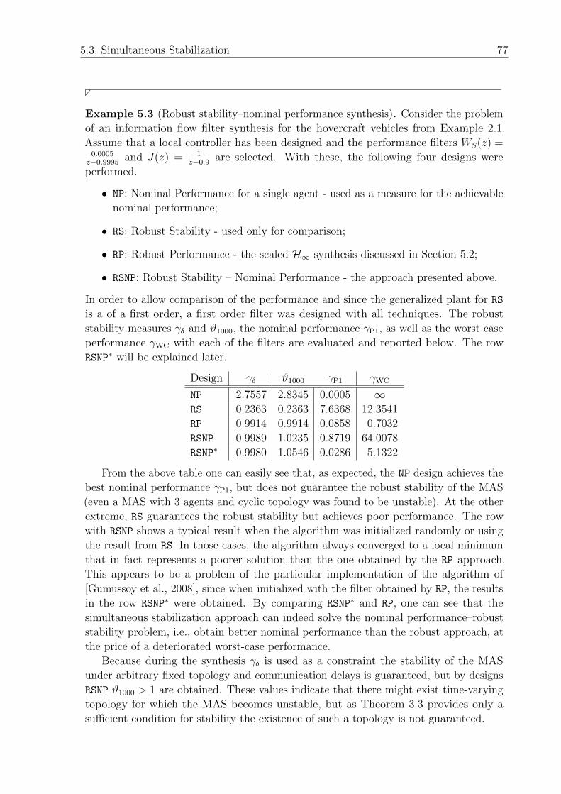
5.3. Simultaneous Stabilization 77
Example 5.3 (Robust stability–nominal performance synthesis). Consider the problem
of an information flow filter synthesis for the hovercraft vehicles from Example 2.1.
Assume that a local controller has been designed and the performance filters WS(z) =0.0005z−0.9995
and J(z) = 1z−0.9
are selected. With these, the following four designs were
performed.
• NP: Nominal Performance for a single agent - used as a measure for the achievable
nominal performance;
• RS: Robust Stability - used only for comparison;
• RP: Robust Performance - the scaled H∞ synthesis discussed in Section 5.2;
• RSNP: Robust Stability – Nominal Performance - the approach presented above.
In order to allow comparison of the performance and since the generalized plant for RS
is a of a first order, a first order filter was designed with all techniques. The robust
stability measures γδ and ϑ1000, the nominal performance γP1, as well as the worst case
performance γWC with each of the filters are evaluated and reported below. The row
RSNP∗ will be explained later.
Design γδ ϑ1000 γP1 γWC
NP 2.7557 2.8345 0.0005 ∞RS 0.2363 0.2363 7.6368 12.3541
RP 0.9914 0.9914 0.0858 0.7032
RSNP 0.9989 1.0235 0.8719 64.0078
RSNP∗ 0.9980 1.0546 0.0286 5.1322
From the above table one can easily see that, as expected, the NP design achieves the
best nominal performance γP1, but does not guarantee the robust stability of the MAS
(even a MAS with 3 agents and cyclic topology was found to be unstable). At the other
extreme, RS guarantees the robust stability but achieves poor performance. The row
with RSNP shows a typical result when the algorithm was initialized randomly or using
the result from RS. In those cases, the algorithm always converged to a local minimum
that in fact represents a poorer solution than the one obtained by the RP approach.
This appears to be a problem of the particular implementation of the algorithm of
[Gumussoy et al., 2008], since when initialized with the filter obtained by RP, the results
in the row RSNP∗ were obtained. By comparing RSNP∗ and RP, one can see that the
simultaneous stabilization approach can indeed solve the nominal performance–robust
stability problem, i.e., obtain better nominal performance than the robust approach, at
the price of a deteriorated worst-case performance.
Because during the synthesis γδ is used as a constraint the stability of the MAS
under arbitrary fixed topology and communication delays is guaranteed, but by designs
RSNP ϑ1000 > 1 are obtained. These values indicate that there might exist time-varying
topology for which the MAS becomes unstable, but as Theorem 3.3 provides only a
sufficient condition for stability the existence of such a topology is not guaranteed.
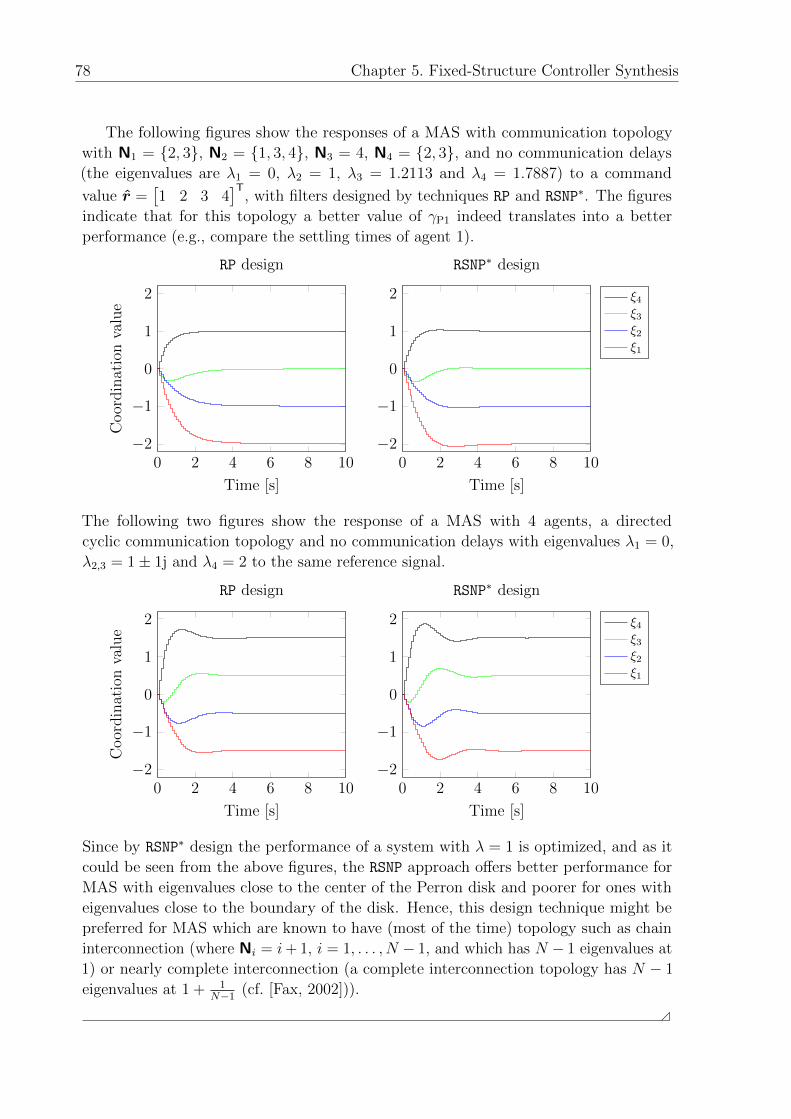
78 Chapter 5. Fixed-Structure Controller Synthesis
The following figures show the responses of a MAS with communication topology
with N1 = {2, 3}, N2 = {1, 3, 4}, N3 = 4, N4 = {2, 3}, and no communication delays
(the eigenvalues are λ1 = 0, λ2 = 1, λ3 = 1.2113 and λ4 = 1.7887) to a command
value r =[1 2 3 4
]T, with filters designed by techniques RP and RSNP∗. The figures
indicate that for this topology a better value of γP1 indeed translates into a better
performance (e.g., compare the settling times of agent 1).
0 2 4 6 8 10−2
−1
0
1
2
Time [s]
Coor
din
atio
nva
lue
RP design
0 2 4 6 8 10−2
−1
0
1
2
Time [s]
RSNP∗ design
ξ4ξ3ξ2ξ1
The following two figures show the response of a MAS with 4 agents, a directed
cyclic communication topology and no communication delays with eigenvalues λ1 = 0,
λ2,3 = 1± 1j and λ4 = 2 to the same reference signal.
0 2 4 6 8 10−2
−1
0
1
2
Time [s]
Coor
din
atio
nva
lue
RP design
0 2 4 6 8 10−2
−1
0
1
2
Time [s]
RSNP∗ design
ξ4ξ3ξ2ξ1
Since by RSNP∗ design the performance of a system with λ = 1 is optimized, and as it
could be seen from the above figures, the RSNP approach offers better performance for
MAS with eigenvalues close to the center of the Perron disk and poorer for ones with
eigenvalues close to the boundary of the disk. Hence, this design technique might be
preferred for MAS which are known to have (most of the time) topology such as chain
interconnection (where Ni = i+ 1, i = 1, . . . , N − 1, and which has N − 1 eigenvalues at
1) or nearly complete interconnection (a complete interconnection topology has N − 1
eigenvalues at 1 + 1N−1
(cf. [Fax, 2002])).
5.4. Replicated Controller Structure 79
5.4 Replicated Controller Structure
In the previous sections it was demonstrated, that both the nominal performance synthesis
problem (Problem 4.6) and the scaledH∞ synthesis (see Section 5.2) can be reformulated as
an H∞ synthesis of a controller with replicated sub-blocks. Moreover, such controllers with
replicated sub-elements might be needed not only in the distributed controller synthesis
for a MAS, but also when the underlying system has symmetric components or consists of
repeated elements. Examples of such systems are:
• electric cars, Segway personal mobility units, quad-rotor helicopter, etc., where
several actuators should be controlled in an identical manner;
• systems with redundant components – such as the tail-plane of an airplane (see
[Wachendorf et al., 2008; Popov et al., 2010a]), where two motors work in parallel,
sharing the work load and providing increased safety;
• speed-limit control of highways, where each highway segment is controlled in an
identical manner (see, e.g., [Popov et al., 2008]).
As discussed in Section 4.4, the H∞ design of a controller with replicated elements cannot
be expressed as a convex optimization problem. In the following the gradient-based
method for H∞ synthesis is modified to allow it handling a replicated structure inside the
controller.
5.4.1 Design Problem
The H∞ design in Problem 4.6 considers the case when the controller has the structure
Kf(z) = IN ⊗Kf(z). However, in the following a more general structure of the controller
K(z) is considered, since the synthesis principles and the gradient computation remain the
same. Let x1, . . . , xU ∈ R denote the unique controller coefficients and let the controller
be constructed as K(z) =
AK BK
CK DK
, where
AK = AK0 +U∑h=1
PAKh ⊗ xh, BK = BK0 +
U∑h=1
PBKh ⊗ xh,
CK = CK0 +U∑h=1
PCKh ⊗ xh, DK = DK0 +
U∑h=1
PDKh ⊗ xh,
and PAK1 , . . . , PDK
U are pattern matrices, with appropriate dimensions defining how the
controller coefficients are substituted in the controller matrices. Note that, as in this case
xh are scalars, the Kronecker product is equivalent to the usual product of a matrix and a
scalar. However, the same approach can be used also when the controller coefficients xhare matrices.
One can now define the synthesis problem as
minimizeK(z)∈K(z)
‖G(z), K(z)‖∞,
80 Chapter 5. Fixed-Structure Controller Synthesis
where G(z) is the generalized plant. In order to solve this minimization problem using a
gradient-based algorithm, one needs to be able to perform the following calculations:
1. For given coefficients x1, . . . , xU obtain the controller K(z) – this can be performed
by direct substitution in the above equalities for AK , . . . , DK ;
2. Calculate the H∞ norm f of the closed-loop system, and obtain its gradient w.r.t.
the controller matrices AK , . . . , DK – these computations are readily available with
both gradient and sub-gradient techniques [Burke et al., 2006a; Apkarian and Noll,
2006b] (see Appendices C.2 and C.3);
3. Compute the gradient of f w.r.t. the controller coefficients x1, . . . , xU ;
4. Using the obtained gradients, update the controller coefficients.
From the above steps only step three is not readily available and hence, the necessary
computation will be derived in the following.
5.4.2 Gradient Computation
The following theorem is instrumental in obtaining the gradient with respect to the
elements of a controller with replicated structure. The theorem addresses the case, when
only one pattern matrix is present, but the result is later generalized.
Theorem 5.2. Given functions A(x) = A0 + P ⊗ x : R → Rn×m and a differentiable
function f(A(x)) : Rn×m → R, where x ∈ R; A0, P ∈ Rn×m and P is a pattern matrix.
Let ∇Af (the matrix-gradient of f with respect to the elements of A) be known. Then the
gradient of f with respect to x is
∇xf =n∑i=1
m∑k=1
Pik∂f
∂Aik. (5.33)
Proof. Let ei denote column i of In, and ek column k of Im. Note that
P ⊗ x =n∑i=1
m∑k=1
ei (Pikx) eTk .
Applying the chain rule (see Appendix B.2) for a single element B(x) = ei (Pik x) eTk of the
above double sum provides
∇xf = 〈∇Bf , ∇xB 〉=trace
((∇Bf )T ei Pik eTk
)=trace
(Pik eTk (∇Bf )T ei
)=eTk Pik (∇Bf )T ei.
Then, rewriting
∇Af =n∑i=1
m∑k=1
ei∂f
∂AikeTk
5.4. Replicated Controller Structure 81
and using that eTk ek = 1, the matrix gradient with respect to x is obtained:
∇xf = 〈∇Af , ∇xA 〉
=trace
(n∑i=1
m∑k=1
ek
(∂f
∂Aik
)T
eTi
n∑i=1
m∑k=1
eiPikeTk
)
=trace
(n∑i=1
m∑k=1
eTk ek Pik∂f
∂AikeTi ei
)
=n∑i=1
m∑k=1
Pik∂f
∂Aik.
�
The above theorem states that the gradient of f w.r.t. x is the sum of the elements of
the matrix gradient of f w.r.t. A, weighted by the corresponding elements in the pattern
matrix.
As an example, consider that the controller coefficients x1, . . . , xl, (l ≤ U) are involved
only in the system matrix AK of the controller:
AK = AK0 +l∑
h=1
PAKh ⊗ xh,
and that one wants to compute the gradient of the closed-loop H∞ norm f w.r.t. to those
coefficients. Assume further, that the gradient of f w.r.t. AK is known (see Appendix
C.2). Then the gradient of f w.r.t. xr, ∀r ∈ [1, l] is given by the sum of the elements of
AK , scaled by the corresponding PAKh elements:
∇xrf =n∑i=1
m∑k=1
PAKrik
∂f
∂AKik.
5.4.3 Nominal Performance Design for a MAS
The main drawback of solving Problem 4.6 using the above technique is that the H∞ norm
of a large-scale system FL(G(z), IN ⊗Kf (z)) has to be evaluated, which is computationally
expensive for systems with a large number of agents. Although the cost of a singleH∞ norm
evaluation cannot be reduced without either increasing the conservativeness of the design
or/and loosing the guarantees of the closed-loop performance, one can significantly reduce
the required number of closed-loop H∞ norm evaluations by an appropriate initialization
of the optimization technique.
Both the decomposition-based approach in [Massioni and Verhaegen, 2009] and the
robust design technique presented in Section 4.2 can be used for obtaining an initial
controller. However, the latter one is preferred since:
• The robust approach guarantees the stability under arbitrary topology and communi-
cation delays and the initialization step needs not be repeated when the topology is
changed and a new controller needs to be synthesized. Furthermore, as a stabilizing
82 Chapter 5. Fixed-Structure Controller Synthesis
controller is sufficient for initialization, one can impose weak performance filters and
solve a non-scaled H∞ synthesis problem. If no structural restrictions are imposed
on the controller this problem can be solved as an LMI problem.
• The approach in [Massioni and Verhaegen, 2009] does not account for the structure
of δIp and (for a general L) requires an LMI problem of at least 3 times the size of
the corresponding LMI by non-scaled H∞ synthesis with the robust performance
approach. Indeed, this can be reduced to LMI conditions for only 2 vertices in the
case of topology with only real eigenvalue (e.g., an undirected one), but this is valid
only in the absence of communication delays (cf. Section 3.4).
• The approach in [Massioni and Verhaegen, 2009] cannot be used for synthesis of
fixed-structure controllers, i.e., when Kf(z) ∈ Kf (z).
Example 5.4 (Nominal performance design of an information filter). Consider again the
information flow filter design for hovercraft vehicles discussed in Example 5.2, but assume
that the topology is fixed and known. With the choice J(z) = 1, WS(z) = 0.009995(z−0.999)(z−0.9)
a filter FRS(z) guaranteeing robust stability (γδ = 0.9986) has been designed. The
transfer function of the filter is
FRS(z) =0.67868(z − 0.0908)
(z − 0.1017)(z − 0.999).
The scaled closed-loop H∞ value with this filter is γRP = 1.0305 and the actual worst
case performance, evaluated using the skewed scaled H∞ norm, is γWC = 5.0094.
Now, consider that it is known that the topology is:
T1 Undirected cyclic topology with six agents and no communication delays, i.e.,
Ni = {i − 1, i + 1}, i = 2, . . . , 5, N1 = {6, 2}, N6 = {5, 1}. Applying the above
obtained filter FRS(z) to this topology leads to a performance index of 0.1444 (i.e.,
the closed-loop H∞ norm from v to w in Figure 4.6). Using the above described
method a nominal controller synthesis has been performed, and a filter
FT1(z) =0.75219(z + 0.3913)
(z − 0.213)(z − 1)
obtained. The nominal performance index of this filter on the above topology
is γNP = 0.0744, which is 50% smaller than the one with FRS(z). Note that the
integral behaviour of this filter is obtained as a result of the synthesis process and
is not explicitly required;
T2 Directed cyclic topology with six agents and no communication delays, i.e., Ni =
{i − 1}, i = 2, . . . , 6, N1 = {6}. The robust performance filter for this topology
achieves a performance index of 0.1467. A nominal performance filter for this
topology has been designed and achieves γNP = 0.1178. The transfer function of
the filter is
FT2(z) =0.91004(z − 0.1842)
(z − 0.1283)(z − 0.9997).
5.4. Replicated Controller Structure 83
T3 A topology with seven agents, where agents 1 to 6 are interconnected as in topology
T1 above, but with two steps communication-delay, and where an undirected
communication links with one step communication delay exist between agent 7
and all other agents. The longer communication delays between agents 1 to 6
could be due, for example, to a communication structure in which agent 7 in fact
re-transmits the communicated signals.
The H∞ performance of the robust filter on this topology is 0.1471. With a nominal
performance filter designed for this topology, a performance index of γNP = 0.0702
has been achieved. The transfer function of the filter is
FT3(z) =1.1264(z − 0.3349)
(z − 0.4791)(z − 1).
As can be clearly seen from the above example, the introduced nominal performance
design can be used to achieve a better performance for a given topology than the robust
performance design. However, one should bear in mind that, since the obtained filters
are tailored for a particular topology, they do not (in general) guarantee the stability of
a MAS with a different topology. Furthermore, as the computation of the H∞ norm of
the closed-loop MAS with performance filter is computationally expensive for MAS with
large number of agents or higher order dynamics, this approach is limited to MAS with
moderate number of agents.
Publications
The modifications to the gradient-based algorithm for discrete-time fixed-structure H∞synthesis, discussed in Section 5.1, are implemented as a toolbox for Matlab and published in
[Popov et al., 2010b]. The paper also demonstrates that the proposed method outperforms
several other discrete-time fixed-structure synthesis methods [Farag and Werner, 2005; Hol
et al., 2003] on an active suspension system benchmark control problem published in the
European Journal of Control [Landau et al., 2003].
The necessary gradient modifications for H∞ synthesis of controllers with replicated
elements has been presented in [Popov and Werner, 2010], where it has been shown on the
problem of a controller synthesis for a satellite constellation that the replicated controller
synthesis can achieve better performance than controller of the same order obtained by
the robust performance or the decomposition approaches.

This page is intentionally left blank for pagination.
Chapter 6
Simultaneous Synthesis of Consensus
and Cooperation Modules
And now for something completely different.
Monty Python
In the previous chapters the problems of syntheses of a controller K(z) or an information
flow filter F (z) that robustly stabilizes a MAS were formulated and solved as H∞ synthesis
problems, where an a posteriory check of the l1-norm was used to verify the stability of the
MAS under unknown and switching topology with communication delays. This chapter
uses a formation of hovercrafts as an example on which the two frameworks – cooperative
control and consensus-based control – are compared. It is then shown that although F (z)
and C(z) can be designed independently, there are advantages when they are designed
simultaneously. It is shown how such a design can be performed and, moreover, how one
can use the techniques, developed in this thesis, to design a single control block containing
both the consensus and the cooperation modules in Figure 1.1.
Recall that in terms of the cooperative control framework introduced in [Fax and
Murray, 2004] the cooperation module corresponds to the controller K(z) in Figure 2.1, in
the consensus module only an error averaging takes place (eq. 2.7), and only the output
signals yi are exchanged between the agents. In terms of the consensus-based framework,
the local controller C(z) plays the role of the cooperation module, the averaging of the
error signals and the information flow filter F (z) constitute the consensus module (see
Figure 2.6), and only coordination variables ξi, but no output signals, are communicated
between the agents.
For the purpose of comparison, here the problem of formation control of a MAS of
hovercraft vehicles, with dynamic model given in Example 2.1, is considered. The design
task is to synthesize a control algorithm that guarantees the stability of a MAS of such
vehicles under unknown and switching topology and communication delays. In order to
allow fair comparison between the control strategies, it is assumed that the order of the
control algorithm (that is either the order of K(z) by the cooperative control approach, or
the sum of the orders of F (z) and C(z) by the information flow approach) should be four,
where as discussed in Section 2.3, the information flow filter should be strictly proper.
85
86 Chapter 6. Simultaneous Synthesis of Consensus and Cooperation Modules
Additionally, it is required that the control signal ui of a single vehicle to an unit step
reference command and to an unit step output disturbance should not exceed 5 units.
Remark 6.1. Note, that since a scaled H∞ problem will be solved, a controller synthesis
is only guaranteed to converge to a local minima, even without the restriction on the order
of the control algorithm.
The following two scenarios will be used to illustrate the features of the different
approaches to cooperative vehicle control:
S1 The response of a single agent to an unit step reference command and to an unit step
output disturbance. In the case of a reference command and the cooperative control
framework of Fax and Murray [2004], the controller K(z) of the agent receives the
signals (r − y) and φ as inputs. In the consensus-based framework the information
flow filter F (z) receives the signal r − ξ as input.
S2 The response of a MAS with seven agents and a directed topology with Ni = {i+ 1},i = 1, 2, 4, 5, 6, N7 = {1}, N3 = {4, 7}, with one sample time communication delays in
all channels, to a command signal r =[1 2 3 4 5 6 7
]T, as well as a response
to a unit step output disturbance applied to the output y7 of vehicle seven at time
t = 10 s. Due to the absence of a leader-agent in this topology, the y-positions of the
hovercrafts should converge to r + χ for some χ ∈ R. This topology is selected since
it is very similar to a cyclic topology (i.e., N3 = {4}) which allows easy observation
of effect of oscillations and disturbance propagations, but at the same time is not
symmetric, which avoids cancellations of error signals.
As a detailed design and tuning of a controller for hovercraft vehicles is outside the
scope of this work, the comparison of the different control strategies is made qualitative
rather than quantitative. Nevertheless, the following measures are used as indicators of
the achieved performance:
• Steady-state error ε20 measured as the largest distance error between any two vehicles
in the formation to the commanded signal after 20 seconds and no output disturbance;
• Convergence time tc [s], measured as the longest time from among all the agents for
convergence within an interval of 0.05 units from the final position (assuming no
output disturbances).
In what follows, the different controller designs will be referred by the bold-faced names
listed in square brackets.
6.1 Cooperative Controller Synthesis
A controller K(z) for cooperative vehicle control using the framework of Fax and Murray
[2004] has been designed using the robust-performance controller synthesis [RPK]approach
discussed in Section 4.2. The generalized plant G(z) is as in Figure 4.5, and a sensitivity
shaping filter WS(z) = 0.1z−0.9999
is used. The responses to scenarios S1 and S2 are shown
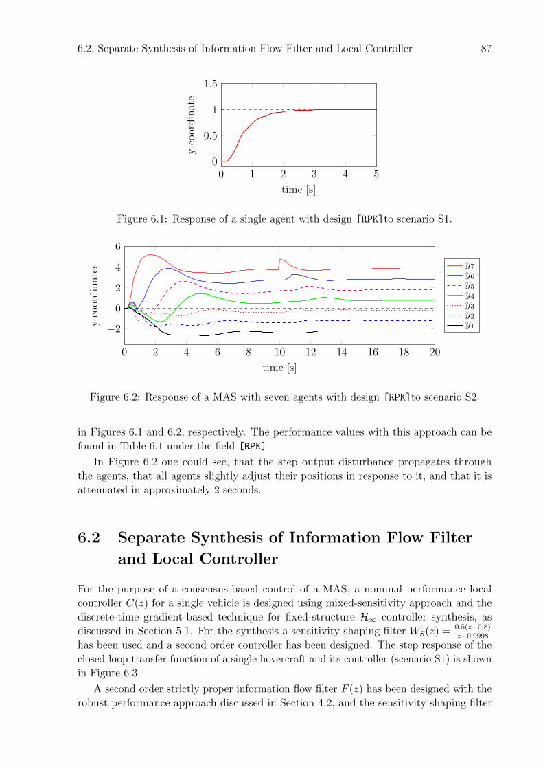
6.2. Separate Synthesis of Information Flow Filter and Local Controller 87
0 1 2 3 4 50
0.5
1
1.5
time [s]y-c
oor
din
ate
Figure 6.1: Response of a single agent with design [RPK]to scenario S1.
0 2 4 6 8 10 12 14 16 18 20
−2
0
2
4
6
time [s]
y-c
oor
din
ates
y7y6y5y4y3y2y1
Figure 6.2: Response of a MAS with seven agents with design [RPK]to scenario S2.
in Figures 6.1 and 6.2, respectively. The performance values with this approach can be
found in Table 6.1 under the field [RPK].
In Figure 6.2 one could see, that the step output disturbance propagates through
the agents, that all agents slightly adjust their positions in response to it, and that it is
attenuated in approximately 2 seconds.
6.2 Separate Synthesis of Information Flow Filter
and Local Controller
For the purpose of a consensus-based control of a MAS, a nominal performance local
controller C(z) for a single vehicle is designed using mixed-sensitivity approach and the
discrete-time gradient-based technique for fixed-structure H∞ controller synthesis, as
discussed in Section 5.1. For the synthesis a sensitivity shaping filter WS(z) = 0.5(z−0.8)z−0.9998
has been used and a second order controller has been designed. The step response of the
closed-loop transfer function of a single hovercraft and its controller (scenario S1) is shown
in Figure 6.3.
A second order strictly proper information flow filter F (z) has been designed with the
robust performance approach discussed in Section 4.2, and the sensitivity shaping filter
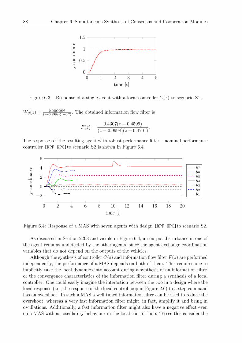
88 Chapter 6. Simultaneous Synthesis of Consensus and Cooperation Modules
0 1 2 3 4 50
0.5
1
1.5
time [s]
y-c
oor
din
ate
Figure 6.3: Response of a single agent with a local controller C(z) to scenario S1.
WS(z) = 0.00099995(z−0.9999)(z−0.7)
. The obtained information flow filter is
F (z) =0.4307(z + 0.4599)
(z − 0.9998)(z + 0.4701).
The responses of the resulting agent with robust performance filter – nominal performance
controller [RPF-NPC]to scenario S2 is shown in Figure 6.4.
0 2 4 6 8 10 12 14 16 18 20
−2
0
2
4
6
time [s]
y-c
oor
din
ates
y7y6y5y4y3y2y1
Figure 6.4: Response of a MAS with seven agents with design [RPF-NPC]to scenario S2.
As discussed in Section 2.3.3 and visible in Figure 6.4, an output disturbance in one of
the agent remains undetected by the other agents, since the agent exchange coordination
variables that do not depend on the outputs of the vehicles.
Although the synthesis of controller C(s) and information flow filter F (z) are performed
independently, the performance of a MAS depends on both of them. This requires one to
implicitly take the local dynamics into account during a synthesis of an information filter,
or the convergence characteristics of the information filter during a synthesis of a local
controller. One could easily imagine the interaction between the two in a design where the
local response (i.e., the response of the local control loop in Figure 2.6) to a step command
has an overshoot. In such a MAS a well tuned information filter can be used to reduce the
overshoot, whereas a very fast information filter might, in fact, amplify it and bring in
oscillations. Additionally, a fast information filter might also have a negative effect even
on a MAS without oscillatory behaviour in the local control loop. To see this consider the
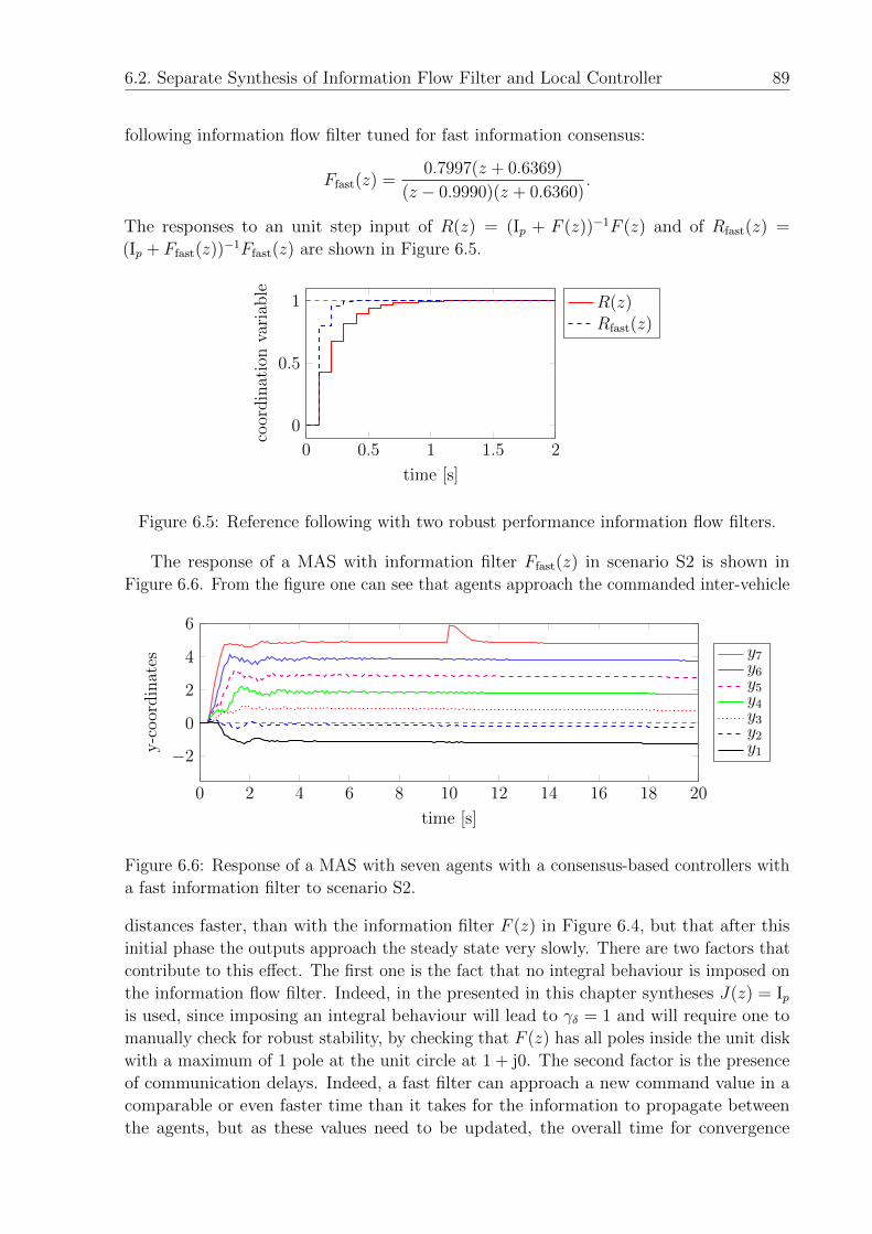
6.2. Separate Synthesis of Information Flow Filter and Local Controller 89
following information flow filter tuned for fast information consensus:
Ffast(z) =0.7997(z + 0.6369)
(z − 0.9990)(z + 0.6360).
The responses to an unit step input of R(z) = (Ip + F (z))−1F (z) and of Rfast(z) =
(Ip + Ffast(z))−1Ffast(z) are shown in Figure 6.5.
0 0.5 1 1.5 2
0
0.5
1
time [s]
coor
din
atio
nva
riab
le
R(z)Rfast(z)
Figure 6.5: Reference following with two robust performance information flow filters.
The response of a MAS with information filter Ffast(z) in scenario S2 is shown in
Figure 6.6. From the figure one can see that agents approach the commanded inter-vehicle
0 2 4 6 8 10 12 14 16 18 20
−2
0
2
4
6
time [s]
y-c
oor
din
ates
y7y6y5y4y3y2y1
Figure 6.6: Response of a MAS with seven agents with a consensus-based controllers with
a fast information filter to scenario S2.
distances faster, than with the information filter F (z) in Figure 6.4, but that after this
initial phase the outputs approach the steady state very slowly. There are two factors that
contribute to this effect. The first one is the fact that no integral behaviour is imposed on
the information flow filter. Indeed, in the presented in this chapter syntheses J(z) = Ipis used, since imposing an integral behaviour will lead to γδ = 1 and will require one to
manually check for robust stability, by checking that F (z) has all poles inside the unit disk
with a maximum of 1 pole at the unit circle at 1 + j0. The second factor is the presence
of communication delays. Indeed, a fast filter can approach a new command value in a
comparable or even faster time than it takes for the information to propagate between
the agents, but as these values need to be updated, the overall time for convergence
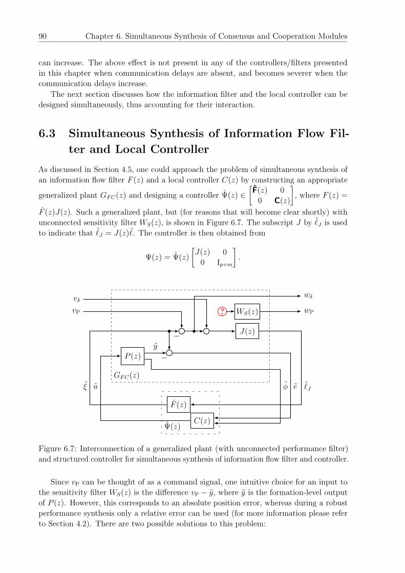
90 Chapter 6. Simultaneous Synthesis of Consensus and Cooperation Modules
can increase. The above effect is not present in any of the controllers/filters presented
in this chapter when communication delays are absent, and becomes severer when the
communication delays increase.
The next section discusses how the information filter and the local controller can be
designed simultaneously, thus accounting for their interaction.
6.3 Simultaneous Synthesis of Information Flow Fil-
ter and Local Controller
As discussed in Section 4.5, one could approach the problem of simultaneous synthesis of
an information flow filter F (z) and a local controller C(z) by constructing an appropriate
generalized plant GFC(z) and designing a controller Ψ(z) ∈[
F(z) 0
0 C(z)
], where F (z) =
F (z)J(z). Such a generalized plant, but (for reasons that will become clear shortly) with
unconnected sensitivity filter WS(z), is shown in Figure 6.7. The subscript J by ˜J is used
to indicate that ˜J = J(z)˜. The controller is then obtained from
Ψ(z) = Ψ(z)
[J(z) 0
0 Ip+m
].
? WS(z)
J(z)
P (z)
F (z)
C(z)
uξ φ e ˜J
−y
−
vδwδ
wPvP
GFC(z)
Ψ(z)
Figure 6.7: Interconnection of a generalized plant (with unconnected performance filter)
and structured controller for simultaneous synthesis of information flow filter and controller.
Since vP can be thought of as a command signal, one intuitive choice for an input to
the sensitivity filter WS(z) is the difference vP − y, where y is the formation-level output
of P (z). However, this corresponds to an absolute position error, whereas during a robust
performance synthesis only a relative error can be used (for more information please refer
to Section 4.2). There are two possible solutions to this problem:
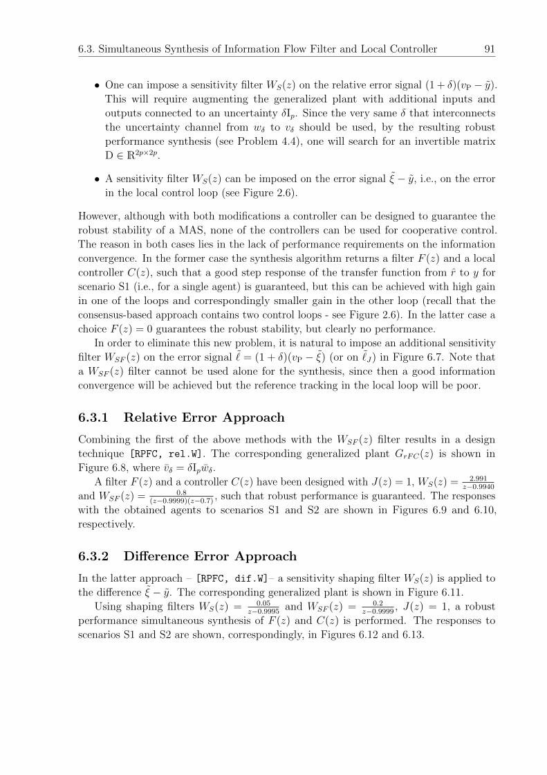
6.3. Simultaneous Synthesis of Information Flow Filter and Local Controller 91
• One can impose a sensitivity filter WS(z) on the relative error signal (1 + δ)(vP − y).
This will require augmenting the generalized plant with additional inputs and
outputs connected to an uncertainty δIp. Since the very same δ that interconnects
the uncertainty channel from wδ to vδ should be used, by the resulting robust
performance synthesis (see Problem 4.4), one will search for an invertible matrix
D ∈ R2p×2p.
• A sensitivity filter WS(z) can be imposed on the error signal ξ − y, i.e., on the error
in the local control loop (see Figure 2.6).
However, although with both modifications a controller can be designed to guarantee the
robust stability of a MAS, none of the controllers can be used for cooperative control.
The reason in both cases lies in the lack of performance requirements on the information
convergence. In the former case the synthesis algorithm returns a filter F (z) and a local
controller C(z), such that a good step response of the transfer function from r to y for
scenario S1 (i.e., for a single agent) is guaranteed, but this can be achieved with high gain
in one of the loops and correspondingly smaller gain in the other loop (recall that the
consensus-based approach contains two control loops - see Figure 2.6). In the latter case a
choice F (z) = 0 guarantees the robust stability, but clearly no performance.
In order to eliminate this new problem, it is natural to impose an additional sensitivity
filter WSF (z) on the error signal ˜= (1 + δ)(vP − ξ) (or on ˜J) in Figure 6.7. Note that
a WSF (z) filter cannot be used alone for the synthesis, since then a good information
convergence will be achieved but the reference tracking in the local loop will be poor.
6.3.1 Relative Error Approach
Combining the first of the above methods with the WSF (z) filter results in a design
technique [RPFC, rel.W]. The corresponding generalized plant GrFC(z) is shown in
Figure 6.8, where vδ = δIpwδ.
A filter F (z) and a controller C(z) have been designed with J(z) = 1, WS(z) = 2.991z−0.9940
and WSF (z) = 0.8(z−0.9999)(z−0.7)
, such that robust performance is guaranteed. The responses
with the obtained agents to scenarios S1 and S2 are shown in Figures 6.9 and 6.10,
respectively.
6.3.2 Difference Error Approach
In the latter approach – [RPFC, dif.W]– a sensitivity shaping filter WS(z) is applied to
the difference ξ − y. The corresponding generalized plant is shown in Figure 6.11.
Using shaping filters WS(z) = 0.05z−0.9995
and WSF (z) = 0.2z−0.9999
, J(z) = 1, a robust
performance simultaneous synthesis of F (z) and C(z) is performed. The responses to
scenarios S1 and S2 are shown, correspondingly, in Figures 6.12 and 6.13.
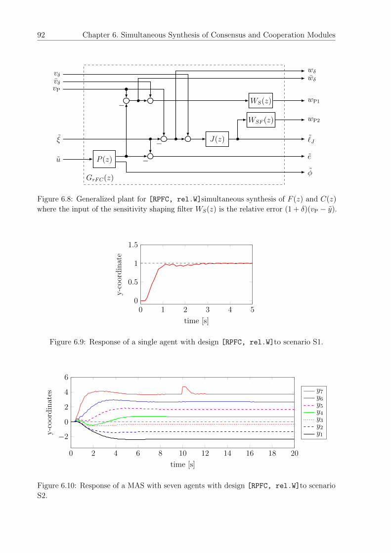
92 Chapter 6. Simultaneous Synthesis of Consensus and Cooperation Modules
WS(z)
WSF (z)
J(z)
P (z)
−
u
ξ
−
wP1
wP2
˜J
e
φ
vδvδ
wδwδ
vP
−
GrFC(z)
Figure 6.8: Generalized plant for [RPFC, rel.W]simultaneous synthesis of F (z) and C(z)
where the input of the sensitivity shaping filter WS(z) is the relative error (1 + δ)(vP − y).
0 1 2 3 4 50
0.5
1
1.5
time [s]
y-c
oor
din
ate
Figure 6.9: Response of a single agent with design [RPFC, rel.W]to scenario S1.
0 2 4 6 8 10 12 14 16 18 20
−2
0
2
4
6
time [s]
y-c
oor
din
ates
y7y6y5y4y3y2y1
Figure 6.10: Response of a MAS with seven agents with design [RPFC, rel.W]to scenario
S2.
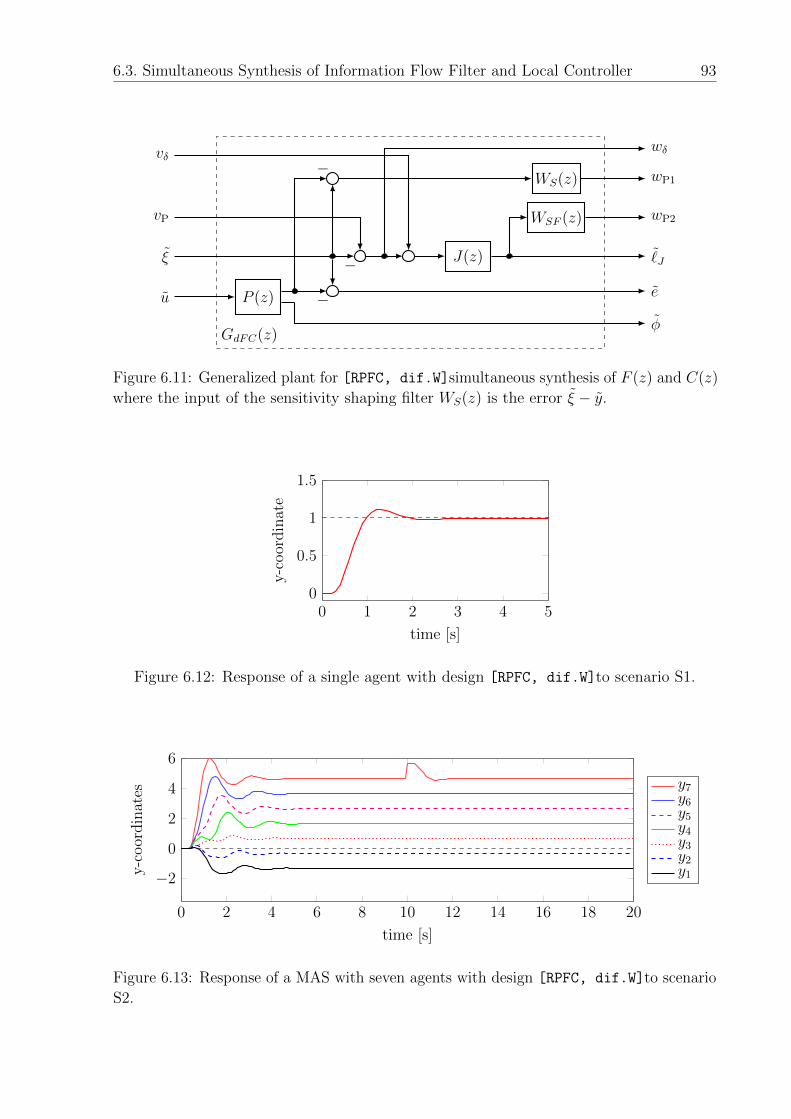
6.3. Simultaneous Synthesis of Information Flow Filter and Local Controller 93
WS(z)
WSF (z)
J(z)
P (z)
−
u
ξ
−
wP1
wP2
˜J
e
φ
vδwδ
vP
−
GdFC(z)
Figure 6.11: Generalized plant for [RPFC, dif.W]simultaneous synthesis of F (z) and C(z)
where the input of the sensitivity shaping filter WS(z) is the error ξ − y.
0 1 2 3 4 50
0.5
1
1.5
time [s]
y-c
oor
din
ate
Figure 6.12: Response of a single agent with design [RPFC, dif.W]to scenario S1.
0 2 4 6 8 10 12 14 16 18 20
−2
0
2
4
6
time [s]
y-c
oor
din
ates
y7y6y5y4y3y2y1
Figure 6.13: Response of a MAS with seven agents with design [RPFC, dif.W]to scenario
S2.
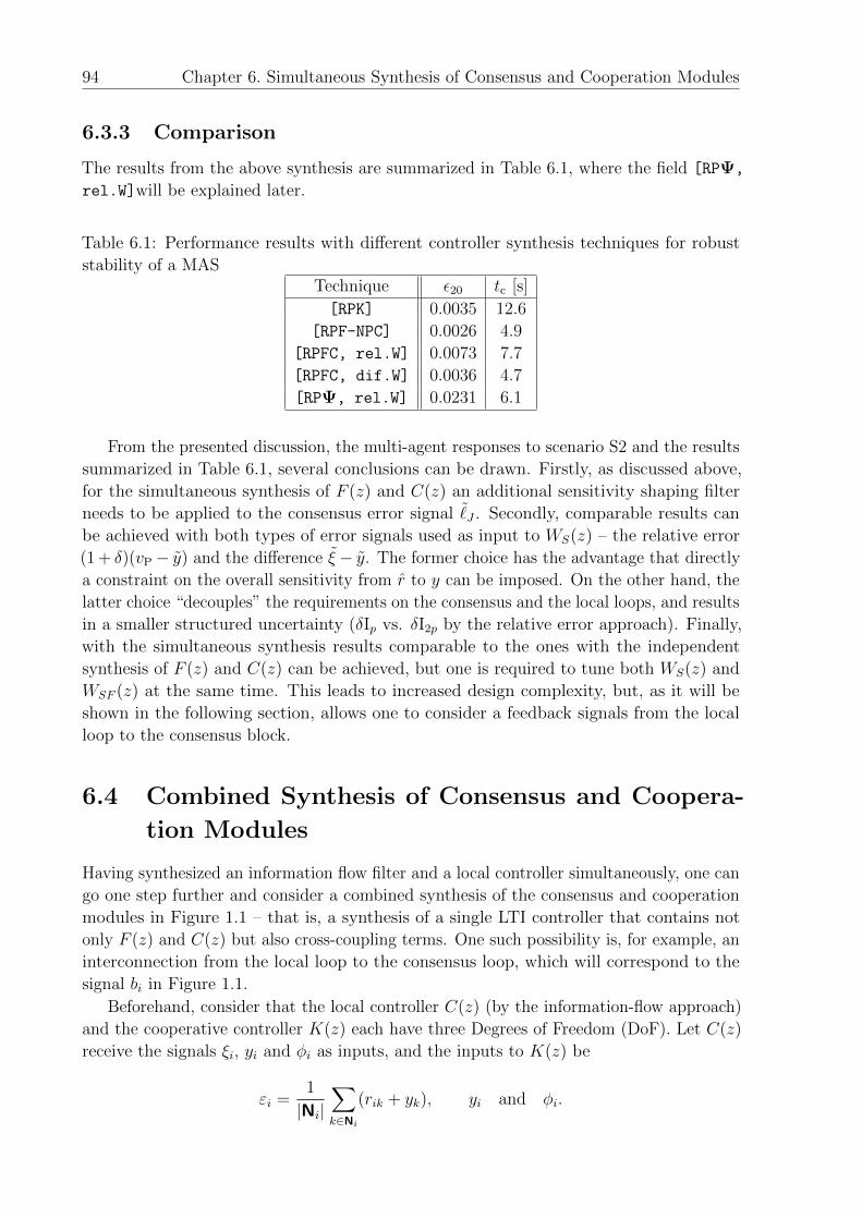
94 Chapter 6. Simultaneous Synthesis of Consensus and Cooperation Modules
6.3.3 Comparison
The results from the above synthesis are summarized in Table 6.1, where the field [RPΨ,
rel.W]will be explained later.
Table 6.1: Performance results with different controller synthesis techniques for robust
stability of a MASTechnique ε20 tc [s]
[RPK] 0.0035 12.6
[RPF-NPC] 0.0026 4.9
[RPFC, rel.W] 0.0073 7.7
[RPFC, dif.W] 0.0036 4.7
[RPΨ, rel.W] 0.0231 6.1
From the presented discussion, the multi-agent responses to scenario S2 and the results
summarized in Table 6.1, several conclusions can be drawn. Firstly, as discussed above,
for the simultaneous synthesis of F (z) and C(z) an additional sensitivity shaping filter
needs to be applied to the consensus error signal ˜J . Secondly, comparable results can
be achieved with both types of error signals used as input to WS(z) – the relative error
(1 + δ)(vP− y) and the difference ξ − y. The former choice has the advantage that directly
a constraint on the overall sensitivity from r to y can be imposed. On the other hand, the
latter choice “decouples” the requirements on the consensus and the local loops, and results
in a smaller structured uncertainty (δIp vs. δI2p by the relative error approach). Finally,
with the simultaneous synthesis results comparable to the ones with the independent
synthesis of F (z) and C(z) can be achieved, but one is required to tune both WS(z) and
WSF (z) at the same time. This leads to increased design complexity, but, as it will be
shown in the following section, allows one to consider a feedback signals from the local
loop to the consensus block.
6.4 Combined Synthesis of Consensus and Coopera-
tion Modules
Having synthesized an information flow filter and a local controller simultaneously, one can
go one step further and consider a combined synthesis of the consensus and cooperation
modules in Figure 1.1 – that is, a synthesis of a single LTI controller that contains not
only F (z) and C(z) but also cross-coupling terms. One such possibility is, for example, an
interconnection from the local loop to the consensus loop, which will correspond to the
signal bi in Figure 1.1.
Beforehand, consider that the local controller C(z) (by the information-flow approach)
and the cooperative controller K(z) each have three Degrees of Freedom (DoF). Let C(z)
receive the signals ξi, yi and φi as inputs, and the inputs to K(z) be
εi =1
|Ni|∑k∈Ni
(rik + yk), yi and φi.
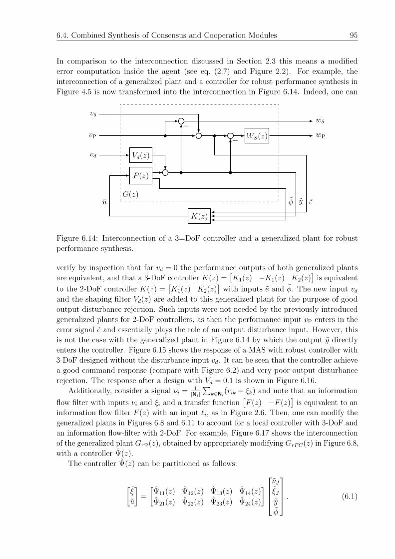
6.4. Combined Synthesis of Consensus and Cooperation Modules 95
In comparison to the interconnection discussed in Section 2.3 this means a modified
error computation inside the agent (see eq. (2.7) and Figure 2.2). For example, the
interconnection of a generalized plant and a controller for robust performance synthesis in
Figure 4.5 is now transformed into the interconnection in Figure 6.14. Indeed, one can
WS(z)
Vd(z)
P (z)
K(z)
φ y εu
vδ
vP
wδ
wP
−−
vd
G(z)
Figure 6.14: Interconnection of a 3=DoF controller and a generalized plant for robust
performance synthesis.
verify by inspection that for vd = 0 the performance outputs of both generalized plants
are equivalent, and that a 3-DoF controller K(z) =[K1(z) −K1(z) K2(z)
]is equivalent
to the 2-DoF controller K(z) =[K1(z) K2(z)
]with inputs e and φ. The new input vd
and the shaping filter Vd(z) are added to this generalized plant for the purpose of good
output disturbance rejection. Such inputs were not needed by the previously introduced
generalized plants for 2-DoF controllers, as then the performance input vP enters in the
error signal e and essentially plays the role of an output disturbance input. However, this
is not the case with the generalized plant in Figure 6.14 by which the output y directly
enters the controller. Figure 6.15 shows the response of a MAS with robust controller with
3-DoF designed without the disturbance input vd. It can be seen that the controller achieve
a good command response (compare with Figure 6.2) and very poor output disturbance
rejection. The response after a design with Vd = 0.1 is shown in Figure 6.16.
Additionally, consider a signal νi = 1|Ni|∑
k∈Ni(rik + ξk) and note that an information
flow filter with inputs νi and ξi and a transfer function[F (z) −F (z)
]is equivalent to an
information flow filter F (z) with an input `i, as in Figure 2.6. Then, one can modify the
generalized plants in Figures 6.8 and 6.11 to account for a local controller with 3-DoF and
an information flow-filter with 2-DoF. For example, Figure 6.17 shows the interconnection
of the generalized plant GrΨ(z), obtained by appropriately modifying GrFC(z) in Figure 6.8,
with a controller Ψ(z).
The controller Ψ(z) can be partitioned as follows:
[ξ
u
]=
[Ψ11(z) Ψ12(z) Ψ13(z) Ψ14(z)
Ψ21(z) Ψ22(z) Ψ23(z) Ψ24(z)
]νJξJy
φ
. (6.1)
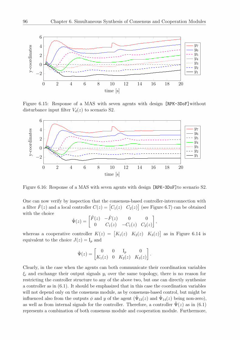
96 Chapter 6. Simultaneous Synthesis of Consensus and Cooperation Modules
0 2 4 6 8 10 12 14 16 18 20
−2
0
2
4
6
time [s]
y-c
oor
din
ates
y7y6y5y4y3y2y1
Figure 6.15: Response of a MAS with seven agents with design [RPK-3DoF]without
disturbance input filter Vd(z) to scenario S2.
0 2 4 6 8 10 12 14 16 18 20
−2
0
2
4
6
time [s]
y-c
oor
din
ates
y7y6y5y4y3y2y1
Figure 6.16: Response of a MAS with seven agents with design [RPK-3DoF]to scenario S2.
One can now verify by inspection that the consensus-based controller-interconnection with
a filter F (z) and a local controller C(z) =[C1(z) C2(z)
](see Figure 6.7) can be obtained
with the choice
Ψ(z) =
[F (z) −F (z) 0 0
0 C1(z) −C1(z) C2(z)
],
whereas a cooperative controller K(z) =[K1(z) K2(z) K3(z)
]as in Figure 6.14 is
equivalent to the choice J(z) = Ip and
Ψ(z) =
[0 0 Ip 0
K1(z) 0 K2(z) K3(z)
].
Clearly, in the case when the agents can both communicate their coordination variables
ξi and exchange their output signals yi over the same topology, there is no reason for
restricting the controller structure to any of the above two, but one can directly synthesize
a controller as in (6.1). It should be emphasized that in this case the coordination variables
will not depend only on the consensus module, as by consensus-based control, but might be
influenced also from the outputs φ and y of the agent (Ψ13(z) and Ψ14(z) being non-zero),
as well as from internal signals for the controller. Therefore, a controller Ψ(z) as in (6.1)
represents a combination of both consensus module and cooperation module. Furthermore,
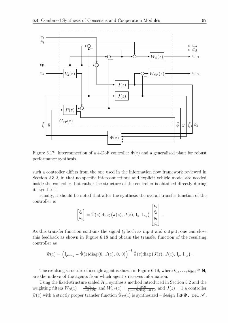
6.4. Combined Synthesis of Consensus and Cooperation Modules 97
WS(z)
Vd(z) WSF (z)
J(z)
J(z)
P (z)
Ψ(z)
φ y ξJ νJuξ
vδ
vP
wδvδ
wδwP1
wP2
−
−
vd −
GrΨ(z)
Figure 6.17: Interconnection of a 4-DoF controller Ψ(z) and a generalized plant for robust
performance synthesis.
such a controller differs from the one used in the information flow framework reviewed in
Section 2.3.2, in that no specific interconnections and explicit vehicle model are needed
inside the controller, but rather the structure of the controller is obtained directly during
its synthesis.
Finally, it should be noted that after the synthesis the overall transfer function of the
controller is [ξiui
]= Ψ(z) diag
(J(z), J(z), Ip, Inφ
)νiξiyiφi
.As this transfer function contains the signal ξi both as input and output, one can close
this feedback as shown in Figure 6.18 and obtain the transfer function of the resulting
controller as
Ψ(z) =(
Ip+nu − Ψ(z)diag (0, J(z), 0, 0))−1
Ψ(z)diag(J(z), J(z), Ip, Inφ
).
The resulting structure of a single agent is shown in Figure 6.19, where k1, . . . , k|Ni| ∈ Ni
are the indices of the agents from which agent i receives information.
Using the fixed-structure scaled H∞ synthesis method introduced in Section 5.2 and the
weighting filters WS(z) = 0.0012z−0.9999
and WSF (z) = 0.1999(z−0.9990)(z−0.7)
, and J(z) = 1 a controller
Ψ(z) with a strictly proper transfer function Ψ12(z) is synthesized – design [RPΨ, rel.W].
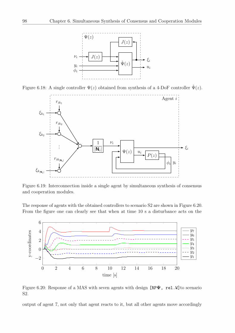
98 Chapter 6. Simultaneous Synthesis of Consensus and Cooperation Modules
Ψ(z)
J(z)
ξi
ui
J(z)νi
yiφi
Ψ(z)
Figure 6.18: A single controller Ψ(z) obtained from synthesis of a 4-DoF controller Ψ(z).
Ψ(z)P (z)
1
|Ni|...
rik2
ξk2
rik1
ξk1
rik|Ni|
ξk|Ni|
φi yi
νi
uiξi
Agent i
Figure 6.19: Interconnection inside a single agent by simultaneous synthesis of consensus
and cooperation modules.
The response of agents with the obtained controllers to scenario S2 are shown in Figure 6.20.
From the figure one can clearly see that when at time 10 s a disturbance acts on the
0 2 4 6 8 10 12 14 16 18 20
−2
0
2
4
6
time [s]
y-c
oor
din
ates
y7y6y5y4y3y2y1
Figure 6.20: Response of a MAS with seven agents with design [RPΨ, rel.W]to scenario
S2.
output of agent 7, not only that agent reacts to it, but all other agents move accordingly
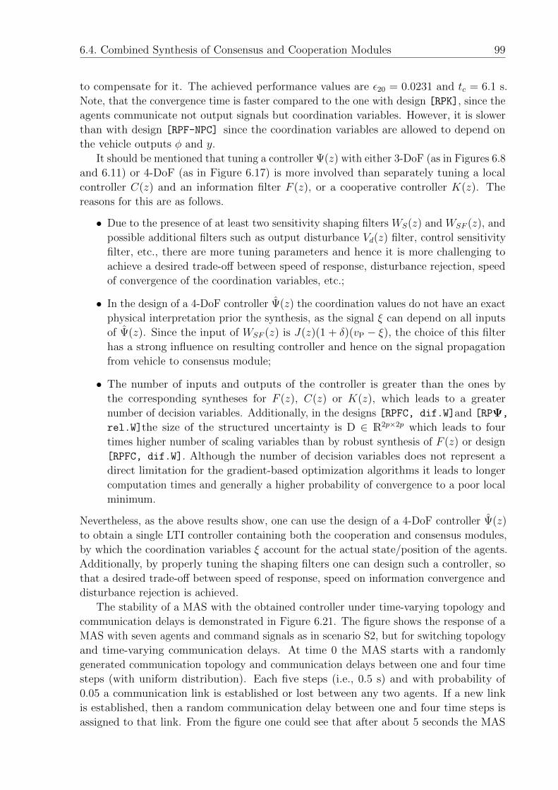
6.4. Combined Synthesis of Consensus and Cooperation Modules 99
to compensate for it. The achieved performance values are ε20 = 0.0231 and tc = 6.1 s.
Note, that the convergence time is faster compared to the one with design [RPK], since the
agents communicate not output signals but coordination variables. However, it is slower
than with design [RPF-NPC] since the coordination variables are allowed to depend on
the vehicle outputs φ and y.
It should be mentioned that tuning a controller Ψ(z) with either 3-DoF (as in Figures 6.8
and 6.11) or 4-DoF (as in Figure 6.17) is more involved than separately tuning a local
controller C(z) and an information filter F (z), or a cooperative controller K(z). The
reasons for this are as follows.
• Due to the presence of at least two sensitivity shaping filters WS(z) and WSF (z), and
possible additional filters such as output disturbance Vd(z) filter, control sensitivity
filter, etc., there are more tuning parameters and hence it is more challenging to
achieve a desired trade-off between speed of response, disturbance rejection, speed
of convergence of the coordination variables, etc.;
• In the design of a 4-DoF controller Ψ(z) the coordination values do not have an exact
physical interpretation prior the synthesis, as the signal ξ can depend on all inputs
of Ψ(z). Since the input of WSF (z) is J(z)(1 + δ)(vP − ξ), the choice of this filter
has a strong influence on resulting controller and hence on the signal propagation
from vehicle to consensus module;
• The number of inputs and outputs of the controller is greater than the ones by
the corresponding syntheses for F (z), C(z) or K(z), which leads to a greater
number of decision variables. Additionally, in the designs [RPFC, dif.W]and [RPΨ,
rel.W]the size of the structured uncertainty is D ∈ R2p×2p which leads to four
times higher number of scaling variables than by robust synthesis of F (z) or design
[RPFC, dif.W]. Although the number of decision variables does not represent a
direct limitation for the gradient-based optimization algorithms it leads to longer
computation times and generally a higher probability of convergence to a poor local
minimum.
Nevertheless, as the above results show, one can use the design of a 4-DoF controller Ψ(z)
to obtain a single LTI controller containing both the cooperation and consensus modules,
by which the coordination variables ξ account for the actual state/position of the agents.
Additionally, by properly tuning the shaping filters one can design such a controller, so
that a desired trade-off between speed of response, speed on information convergence and
disturbance rejection is achieved.
The stability of a MAS with the obtained controller under time-varying topology and
communication delays is demonstrated in Figure 6.21. The figure shows the response of a
MAS with seven agents and command signals as in scenario S2, but for switching topology
and time-varying communication delays. At time 0 the MAS starts with a randomly
generated communication topology and communication delays between one and four time
steps (with uniform distribution). Each five steps (i.e., 0.5 s) and with probability of
0.05 a communication link is established or lost between any two agents. If a new link
is established, then a random communication delay between one and four time steps is
assigned to that link. From the figure one could see that after about 5 seconds the MAS
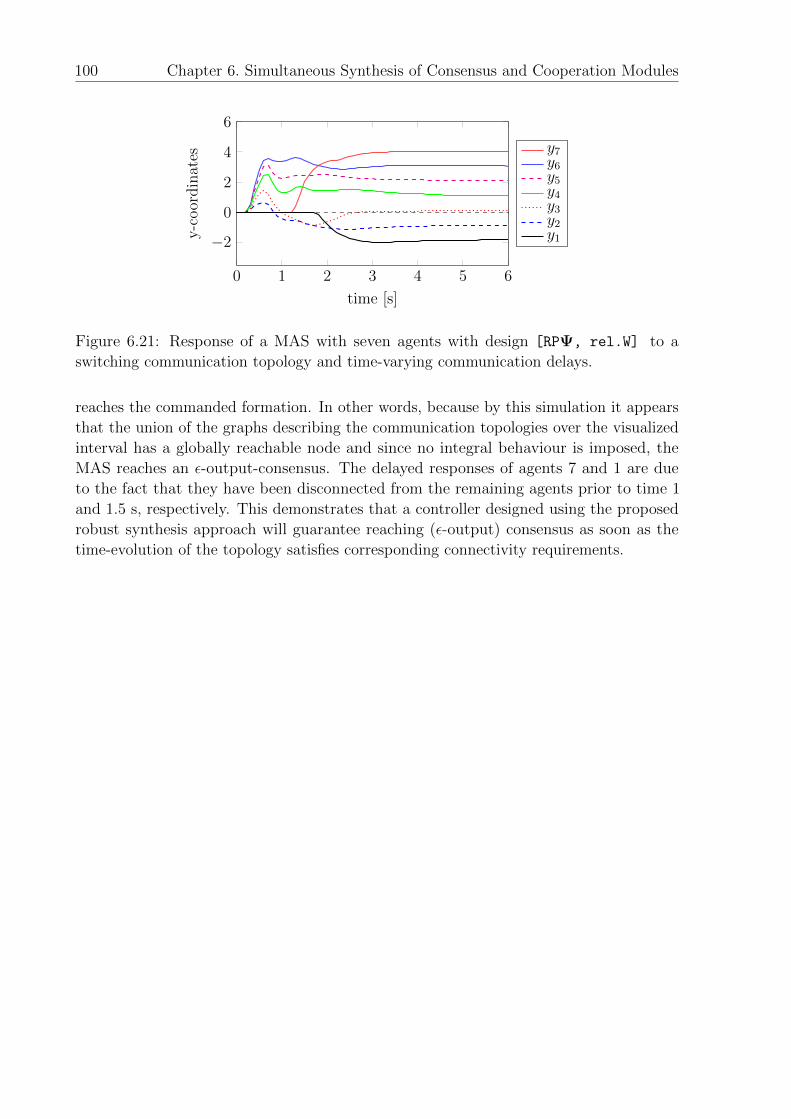
100 Chapter 6. Simultaneous Synthesis of Consensus and Cooperation Modules
0 1 2 3 4 5 6
−2
0
2
4
6
time [s]
y-c
oor
din
ates
y7y6y5y4y3y2y1
Figure 6.21: Response of a MAS with seven agents with design [RPΨ, rel.W] to a
switching communication topology and time-varying communication delays.
reaches the commanded formation. In other words, because by this simulation it appears
that the union of the graphs describing the communication topologies over the visualized
interval has a globally reachable node and since no integral behaviour is imposed, the
MAS reaches an ε-output-consensus. The delayed responses of agents 7 and 1 are due
to the fact that they have been disconnected from the remaining agents prior to time 1
and 1.5 s, respectively. This demonstrates that a controller designed using the proposed
robust synthesis approach will guarantee reaching (ε-output) consensus as soon as the
time-evolution of the topology satisfies corresponding connectivity requirements.
Chapter 7
Summary, Conclusions and Outlook
There is no real ending. Its just the place where
you stop the story.
Frank Herbert
In this thesis the problems of stability analysis and controller synthesis, for the purpose
of cooperative vehicle control under unknown and switching interconnection between the
vehicles and under unknown and time-varying communication delays, were addressed. In
Chapter 2 three different frameworks to cooperative control were reviewed and it was shown
that they can be considered as special cases of a general problem. In Chapter 3 a condition,
that is both necessary and sufficient, for the robust stability of a multi-agent system with
arbitrary number of agents to arbitrary, but fixed, topology and communication delays,
was derived. Additionally, sufficient conditions were obtained for the robust stability of
a MAS under switching topology and time-varying communication delays. In contrast
to previous results, the proposed conditions reduce the stability analysis of a MAS with
arbitrary number of agents and topology to a scaled (by static matrix) l1 or H∞ stability
analysis of a single agent with uncertainty. It was next demonstrated that the stability
analysis can be performed using state of the art semi-definite programming tools (i.e, LMI
solvers). Furthermore, it was shown, that although the obtained condition addresses the
stability of a MAS under arbitrary topologies and communication delays, it represents
a not too conservative test even for a MAS with few agents since the interconnection
topology is rarely exactly known or constant. Finally, it was argued that the proposed
H∞ stability condition is better suited for controller synthesis and that the l1-condition
can be used as an a posteriory verification.
In Chapter 4 the problem of distributed controller synthesis was addressed. Using
the H∞ control framework, it is shown how the obtained analysis results can be applied
to the problem of distributed controller synthesis. In particular, it was shown that by
robust stability design trivial solutions might exist and that performance requirements
need to be imposed. As the resulting robust performance synthesis does not impose
a performance requirement on the closed-loop multi-agent system, but on the transfer
function of a single agent with uncertainty, an alternative design was proposed which
combines nominal performance requirements with robust stability requirements. Moreover,
101
102 Chapter 7. Summary, Conclusions and Outlook
the problem of a nominal performance synthesis for a MAS with known and fixed topology
and communication delays, was also addressed.
Due to the nature of the scaled H∞ synthesis problem and the fact that each agent
uses an identical copy of the same controller the above synthesis problems could not be
solved directly. However, as each of them allowed expression as an H∞ synthesis of a
controller with structural constraints, the fixed-structured H∞ synthesis problem was
addressed in Chapter 5. This problem is of additional interest due to the fact that in
autonomous vehicles often limited energy supply and processing power are available, thus
giving preference to low-order and fixed-structure controllers. It was shown how recent
gradient-based techniques for H∞ controller synthesis can be modified to allow discrete-
time H∞ synthesis of fixed-structured controllers, and how the nominal performance
controller synthesis problem can be solved. Moreover, gradient-based calculations were
derived, which allow µ-synthesis, in general, and statically-scaled H∞ controller design,
in particular, by simultaneous optimization over controller and scalings variables, thus
avoiding the need of iterating over them. Several examples were used to illustrate the
developed techniques and their applications to the cooperative control of group of vehicles.
Finally, in Chapter 6 the developed synthesis tools were applied to a cooperative
controller synthesis and to a consensus-based approach to cooperative control and the
results compared. Based on the obtained results it was demonstrated that there are
advantages in a simultaneous design of the consensus and cooperation modules of the
agents, and it was shown how the design problem can be formulated and how the proposed
synthesis methods can be applied to it. Additionally, it was demonstrated that one could
in fact design a single module encompassing both consensus and cooperation modules, and
the advantages of doing so were outlined.
7.1 Conclusions
Much attention has been given in the last years to the problem of cooperative control
and coordination of vehicle formations. Different sub-problems, control frameworks and
analysis algorithms have been developed. Many researchers have assumed that a controller
for the vehicles or/and a consensus algorithm is provided, and have derived conditions
under which a multi-agent system will reach (output-) consensus, relying on certain
conditions on the interconnection topology between the agents and the communication
delays. At the same time, the proposed controller synthesis methods usually assume
that the interconnection topology is fixed and known, or that (again) it satisfies certain
assumptions.
In contrast to those results and techniques, the approach presented in this thesis
assumes no knowledge of the number of agents in a multi-agent system, the interconnection
topology or the communication delays, and additionally allows them to vary. Naturally,
by taking the size and topology of a multi-agent system as unknown, statements regarding
performance are difficult to make. In contrast, statements regarding stability are fairly
easy to make, as shown by Theorems 3.2, 3.3 and 3.4. The obtained conditions are
computationally attractive, because they reduce the stability analysis of a MAS (with
possibly large number of agents and unknown topology) to analysis of a single agent
7.1. Conclusions 103
with uncertainty. Furthermore, in the case of fixed but unknown topology, the obtained
condition is not only sufficient but also necessary for the stability.
Apparently, applying such a stability test to a system with a known topology or a
topology varying within a known set might be conservative. However, as communication
delays are always present in practice, since varying distances between the vehicles or
environmental features (e.g., communication obstacles) can lead to unpredicted changes
in the topology, and since such problems become more frequent/dominant in MAS with
large number of agents, this conservatism rapidly diminishes. This makes the proposed
robust stability analysis the method of choice in all but the few cases, when a multi-agent
system with moderate number of agents and known topology is considered, and very strict
performance requirements should be met.
The problem of synthesizing controller guaranteeing the robust stability under switching
topologies and communication delays is attacked using H∞ -synthesis techniques. Because
its difficult computation, the l1-norm stability condition is not used during the synthesis
but rather as an a posteriory tool to verify the robust stability. This way, the synthesis
can be performed using state of the art tools and tuning techniques and repeated if the
staled l1-norm condition is not satisfied.
Because treating the topology and the communication delays as unknown prohibits
giving guarantees for the performance of a particular multi-agent system during the
synthesis process, the synthesis techniques proposed in this thesis take a different approach.
Both of the proposed robust performance and robust stability–nominal performance
synthesis techniques address the problem of synthesizing a controller that will guarantee
the robust stability of a MAS and that achieves reasonable performance. Naturally, the
robust-stability–nominal performance approach achieves better performance on topologies
that have eigenvalues close to the center of the Perron disk, whereas the robust performance
approach is better for topologies with eigenvalues close to the boundary of the disk. As
both synthesis techniques provide robust stability, the decision which one to use must
depend on additional knowledge about the multi-agent system. If no such knowledge is
available, the robust performance synthesis should be preferred as it is easier to perform
and guarantees a better worst-case performance.
The proposed nominal performance synthesis offers a technique that can design a
controller for the other extreme case – a multi-agent system with a fixed topology and
communication-delays. Although that the method requires evaluating the performance
of the overall system and is, therefore, applicable mainly to moderate sized MAS, it
represents a powerful design approach, as it can achieve the best performance with the
system. Additionally, it can be applied to design problems outside the field of cooperative
control, where repeated or redundant blocks/elements/actuators are present.
With view of the agent capabilities, a synthesis of a controller K(z) for the cooperative
control framework is the only approach applicable both to MAS with communication
topologies and to MAS with sensing topologies. However, as the controllers by this
framework rely directly on the outputs of their neighbors, the complete vehicle dynamics
are involved in the agent interaction and such MASs achieve slower responses than when a
consensus-based approach is used. A synthesis of either a local controller or an information
flow filter for the consensus-based approach is easy, but as the overall performance will
depend on both of them the designer needs to consider their interaction. Additionally,
104 Chapter 7. Summary, Conclusions and Outlook
as the coordination variables that the agents exchange do not depend on the actual
state/position of the vehicles, the MAS might not be able to reach output consensus (e.g.,
a commanded formation might not be attained due to a disturbance in one of the agents or
not precise initialization of the coordination variables). The proposed combined synthesis
of consensus and cooperation modules (resulting in a single control block) builds upon the
developed synthesis techniques and addresses these problems. Although resulting in an
increased design effort, the approach allows achieving a trade-off between the cooperative
control approach and the consensus-based approach, and thus a trade-off between reference
tracking and agent interaction.
The proposed gradient-based discrete-time fixed-structure H∞ synthesis and the struc-
tured singular value (µ) synthesis by simultaneous search over controller and scaling
coefficients find also applications outside the cooperative vehicle control field. Simple
fixed-structured controllers, that can be easily implemented, that do not pose high
processor requirements, provide high performance even by large sampling times, are pre-
ferred/required not only by autonomous vehicles, but also for control of various systems
and processes. Additionally, the proposed µ-synthesis via simultaneous optimization over
controller and scaling coefficients avoids the need of iterations over the two and guarantees
that the design will converge at least to a local minimum.
In the light of the above, the tools presented in this thesis approach the stability
analysis and controller synthesis for a multi-agent system from point of view of robustness
guarantees, with respect to number of agents, topology and communication delays. This
contributes to the field of cooperative vehicle control in that a simple robust stability
analysis test on a single agent, or respectively a robust synthesis on a generalized plant
obtained from a single agent, can be used to check the stability, or respectively design
a controller that guarantees the stability, of any conceivable multi-agent system with
the considered agents. This not only greatly simplifies the analysis and the synthesis
processes, but combined with the use of established H∞ tuning rules during the synthesis,
allows easy modifications of the structure inside the agents, experimenting with alternative
signals and communicated outputs, as well as straightforward design of simple controllers.
Furthermore, the fact that the approach provides stability guarantees with respect to
communication delays, makes it a method of choice even for multi-agent systems with fixed
number of agents or topology. Moreover, combination of the proposed robust stability–
nominal performance and nominal performance syntheses with the possibility to apply
them to synthesis of information flow filters, cooperative controllers, as well as simultaneous
synthesis of consensus and cooperation blocks, allows applying the proposed techniques
to a large variety of problems and scenarios. In the light of this, the results presented
in this thesis constitute not only efficient robust analysis and synthesis methods, but
enable further research into distributed control, fixed-structure controller synthesis and
cooperative vehicle control.
7.2. Outlook 105
7.2 Outlook
A number of relevant problems, that might be of independent interest or a topic of further
research, could not be covered in this thesis and are, therefore, outlined in this section.
Necessary and Sufficient Conditions for Stability
Theorem 3.2 provides both a necessary and sufficient condition for stability under arbitrary
but fixed topology and communication delays. In contrast, in the case of switching
topology and time-varying communication delays, Theorems 3.3–3.4 provide sufficient but
not necessary conditions to stability and hence can lead to conservative results. Therefore,
it is of interest to explore, whether an alternative approach or statements can be found
that provide both necessity and sufficiency.
Communication Delays
In this thesis it was assumed that the signals obtained at each agent from its neighbors can
be delayed, but that the agent uses its current knowledge of the reference commands and
the own output for building the formation error. The presence and type of communication
delays, however, leads to two problems.
Firstly, as shown in Section 6.2, in the case when no integral action is imposed in
the information flow filter (or the cooperative controller), a “fast” filter can in fact lead
to a slow information convergence. The reason for this is that due to communication
delays, the information filters converge prematurely to values different than the consensus
values and hence, need to update them over and over again. Naturally, one option is to
impose integral or “nearly integral” action in the filter, but this might lead to a slow
filter and hence again to a slow information convergence. Additionally, such “nearly
integral” behaviour can cause problems due to disturbances, not exact initial values for
the cooperation variables, measurement noises, etc. (cf. [Fax and Murray, 2004]). An
alternative might lie in incorporating knowledge of the communication delays actually
present in a MAS during the synthesis (e.g., using information about communication range,
transmission bandwidth, number of agents). For example, if one knows that a typical
communication delay of 2 samples is present, one might add a block z−2 at the output y
of the vehicle during the synthesis (see Figure 4.5). Clearly, such an ad-hoc solution might
not be the best one and other techniques are needed to allow exploiting knowledge on the
maximal communication delay τ , distribution of the communication delay times, etc.
Secondly, one might argue that an error signal rik(t− τik)− yi(t− τik) + yk(t− τik) com-
puted at vehicle i provides a more useful information than rik(t)−yi(t)+yk(t−τik). Hence,
one might want to consider schemes where the own outputs of the agents are appropriately
delayed, i.e., there are self-delays. Such a scheme will require additional memory space for
storing previous values of ri• and yi, and is applicable only to communicated signals, as a
time-stamp on the received signal is needed in order to perform the correct comparison. If
no upper bound on the communication delays is imposed/known, the robust controller
synthesis techniques, proposed in this thesis, cannot be efficiently applied to a MAS with
such an error computation. The reason hinges on the necessary uncertainty model. In
106 Chapter 7. Summary, Conclusions and Outlook
the results presented here, i.e., when there are only communication but no self-delays,
the eigenvalues of the Laplacian rotate around the center of the Perron disk when the
product τikω increases. If self-delays are allowed, delays will be present in the diagonal
elements of L(z) and the eigenvalues of L(z) will rotate around the origin by increased
τiiω. In the unbounded self-delay case, one will need to consider an uncertainty χ, |χ| ≤ 2,
which is very conservative. To see this, recall that in the SISO case a robust stability of a
MAS with unknown but fixed topology requires the Nyquist plot of H(z) to remain right
from the −0.5 line. With the above uncertainty this condition will require the Nyquist
plot of H(z) to remain in a disc with radius 0.5 centered at the origin, which is clearly
very restrictive. A sufficient stability condition, in the case when an upper bound on the
communication delays (respectively own delays) is known, has been in fact proposed in
[Pilz and Werner, 2010]. It is interesting to know, whether a tighter condition also exists
and whether it could be used for a controller synthesis.
Uncertain Agent Dynamics and Heterogeneous Agents
Throughout this thesis it was assumed that the agent dynamics are exactly known and that
all agents are identical. However, due to manufacturing imperfections and approximations
by the modeling and identification this is rarely the case. Nevertheless, model uncertainties
can be easily incorporated into the proposed design techniques by appropriately augmenting
the generalized plants with additional input and outputs.
Additionally, in some cases it might be necessary to deploy agents of different classes,
e.g., wheeled vehicles and UAVs. Such MAS with heterogenous agents have been studied
for dissipative agents in [Hirche and Hara, 2008] and for general linear systems in [Wieland
and Allgower, 2009]. In fact, in two cases one can also use the design techniques developed
in this thesis to cooperative control of heterogenous vehicles. Firstly, if a consensus-based
approach is used, one can design the local controller for each vehicle independently and
then design a common information flow filter for all agents. Secondly, if a different
cooperative control approach is used, but the topology and communication delays are
known and fixed, the proposed nominal controller technique using replicated structure
in the controller can be used. In this case one needs to consider the following controller
structure diag(IN1 ⊗K1(z), IN2 ⊗K1(z), . . . ) and construct the corresponding generalized
plant, where Nk is the number of agents of type k present in the MAS (∑
kNk = N).
Worst Case Performance
As it was discussed in Section 4.2, the proposed robust performance synthesis does not
provide performance guarantees for a MAS but rather for the decomposed systems Mλi(z).
Therefore, it is an interesting question whether by using Schur or Jordan decomposition,
or alternatively under what topologies (or their features), can one obtain an upper bound
on the performance of MAS with the designed controller.
Moreover, as the actual worst case performance for the decomposed systems is γWC, it
appears only natural to minimize γWC rather than γRP (under the condition γδ < 1). In
7.2. Outlook 107
this case Problem 4.4 should be replaced by
minimizeγWC, K(z)
D∈Rp×p, s.t. ∃D−1
γWC
subject to
∥∥∥∥[D 0
0 Inw
]FL (G(z), K(z))
[D−1 0
0 1γWC
Inv
]∥∥∥∥∞< 1.
This problem cannot be solved directly as it contains product of variables. An immediate
difficulty for using a gradient-based technique to this problem is that the decision variables
appear only in the constraint, i.e., when it is satisfied no gradients are available and the
variables cannot be updated. One solution to this problem lies in using a bisection technique
for γWC, but this results again in an iterative synthesis process. Since a solution to this
problem is of interest for general robust performance synthesis problems, it is interesting
to explore whether/how using the recent advances in the gradient-based techniques to H∞synthesis this problem can be posed in an alternative form and solved efficiently.
Collision Avoidance
In this work it was assumed that the agents have no physical dimensions and hence cannot
collide with each other. However, for a real MAS this assumption holds only when the
agents are sufficiently far away from each other. Indeed, using the cooperative control
approach and the simultaneous synthesis of cooperation and consensus modules, proposed
in Chapter 6, one can ensure that disturbances are propagated between the agents so that
it is easier to preserve the desired inter-agent distances, but this does not replace the need
of a collision avoidance scheme.
One approach to address collision avoidance is to consider artificial potential forces
acting between the agents. This approach is usually used by flocking [Olfati-Saber and
Murray, 2002; Tanner et al., 2007], where the vehicles are required to synchronize their
direction of travel and velocities, but where one does not have control over the final
arrangement of the vehicles in the formation. An alternative technique is proposed in
[Chopra et al., 2008], where an artificial potential forces of repulsion are assumed to act only
in the vicinity of the vehicles for the sole purpose of collision avoidance, and the agents are
controlled using cooperative technique as the ones discussed in Chapter 2. The approach
proposed in [Chopra et al., 2008] is applicable to constant and equal communication delays,
and balanced and undirected communication topology. Furthermore, it does not provide
a design of a potential function and controller for a general MAS. Hence, an important
topic of further investigation is a systematic design and integration of a collision avoidance
scheme in the stability and performance analysis, as well as in the cooperative controller
design problem.

This page is intentionally left blank for pagination.
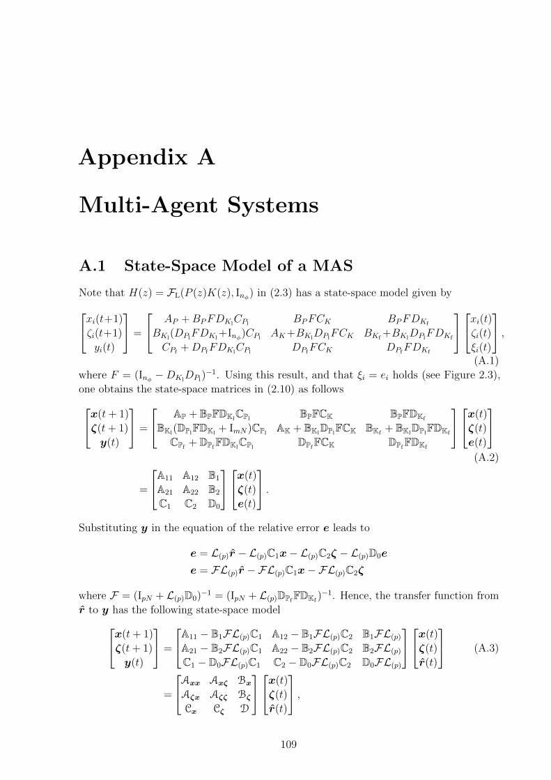
Appendix A
Multi-Agent Systems
A.1 State-Space Model of a MAS
Note that H(z) = FL(P (z)K(z), Inφ) in (2.3) has a state-space model given byxi(t+1)
ζi(t+1)
yi(t)
=
AP +BPFDKlCPl
BPFCK BPFDKf
BKl(DPl
FDKl+Inφ)CPl
AK+BKlDPl
FCK BKf+BKl
DPlFDKf
CPf+DPf
FDKlCPl
DPfFCK DPf
FDKf
xi(t)ζi(t)
ξi(t)
,(A.1)
where F = (Inφ −DKlDPl
)−1. Using this result, and that ξi = ei holds (see Figure 2.3),
one obtains the state-space matrices in (2.10) as followsx(t+ 1)
ζ(t+ 1)
y(t)
=
AP + BPFDKlCPl
BPFCK BPFDKf
BKl(DPl
FDKl+ ImN)CPl
AK + BKlDPl
FCK BKf+ BKl
DPlFDKf
CPf+ DPf
FDKlCPl
DPfFCK DPf
FDKf
x(t)
ζ(t)
e(t)
(A.2)
=
A11 A12 B1
A21 A22 B2
C1 C2 D0
x(t)
ζ(t)
e(t)
.Substituting y in the equation of the relative error e leads to
e = L(p)r − L(p)C1x− L(p)C2ζ − L(p)D0e
e = FL(p)r −FL(p)C1x−FL(p)C2ζ
where F = (IpN + L(p)D0)−1 = (IpN + L(p)DPfFDKf
)−1. Hence, the transfer function from
r to y has the following state-space modelx(t+ 1)
ζ(t+ 1)
y(t)
=
A11 − B1FL(p)C1 A12 − B1FL(p)C2 B1FL(p)
A21 − B2FL(p)C1 A22 − B2FL(p)C2 B2FL(p)
C1 − D0FL(p)C1 C2 − D0FL(p)C2 D0FL(p)
x(t)
ζ(t)
r(t)
(A.3)
=
Axx Axζ BxAζx Aζζ BζCx Cζ D
x(t)
ζ(t)
r(t)
,109
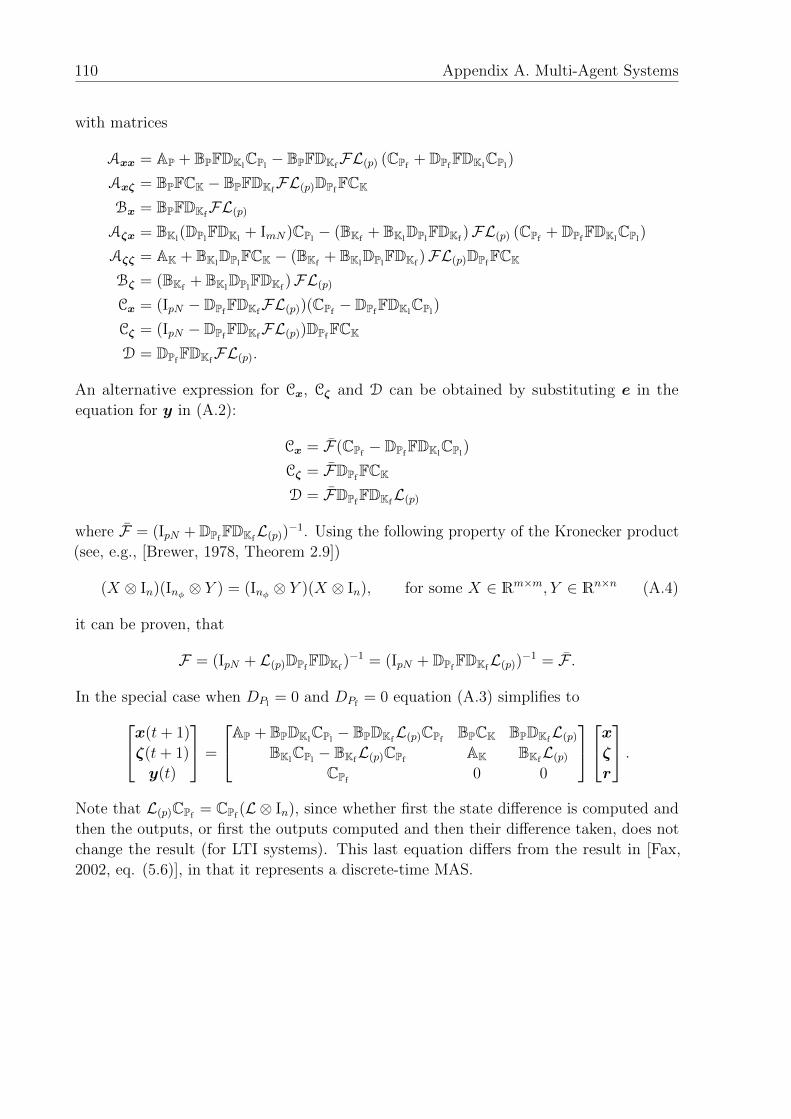
110 Appendix A. Multi-Agent Systems
with matrices
Axx = AP + BPFDKlCPl− BPFDKf
FL(p) (CPf+ DPf
FDKlCPl
)
Axζ = BPFCK − BPFDKfFL(p)DPf
FCK
Bx = BPFDKfFL(p)
Aζx = BKl(DPl
FDKl+ ImN)CPl
− (BKf+ BKl
DPlFDKf
)FL(p) (CPf+ DPf
FDKlCPl
)
Aζζ = AK + BKlDPl
FCK − (BKf+ BKl
DPlFDKf
)FL(p)DPfFCK
Bζ = (BKf+ BKl
DPlFDKf
)FL(p)
Cx = (IpN − DPfFDKf
FL(p))(CPf− DPf
FDKlCPl
)
Cζ = (IpN − DPfFDKf
FL(p))DPfFCK
D = DPfFDKf
FL(p).
An alternative expression for Cx, Cζ and D can be obtained by substituting e in the
equation for y in (A.2):
Cx = F(CPf− DPf
FDKlCPl
)
Cζ = FDPfFCK
D = FDPfFDKf
L(p)
where F = (IpN + DPfFDKf
L(p))−1. Using the following property of the Kronecker product
(see, e.g., [Brewer, 1978, Theorem 2.9])
(X ⊗ In)(Inφ ⊗ Y ) = (Inφ ⊗ Y )(X ⊗ In), for some X ∈ Rm×m, Y ∈ Rn×n (A.4)
it can be proven, that
F = (IpN + L(p)DPfFDKf
)−1 = (IpN + DPfFDKf
L(p))−1 = F .
In the special case when DPl= 0 and DPf
= 0 equation (A.3) simplifies tox(t+ 1)
ζ(t+ 1)
y(t)
=
AP + BPDKlCPl− BPDKf
L(p)CPfBPCK BPDKf
L(p)
BKlCPl− BKf
L(p)CPfAK BKf
L(p)
CPf0 0
xζr
.Note that L(p)CPf
= CPf(L ⊗ In), since whether first the state difference is computed and
then the outputs, or first the outputs computed and then their difference taken, does not
change the result (for LTI systems). This last equation differs from the result in [Fax,
2002, eq. (5.6)], in that it represents a discrete-time MAS.
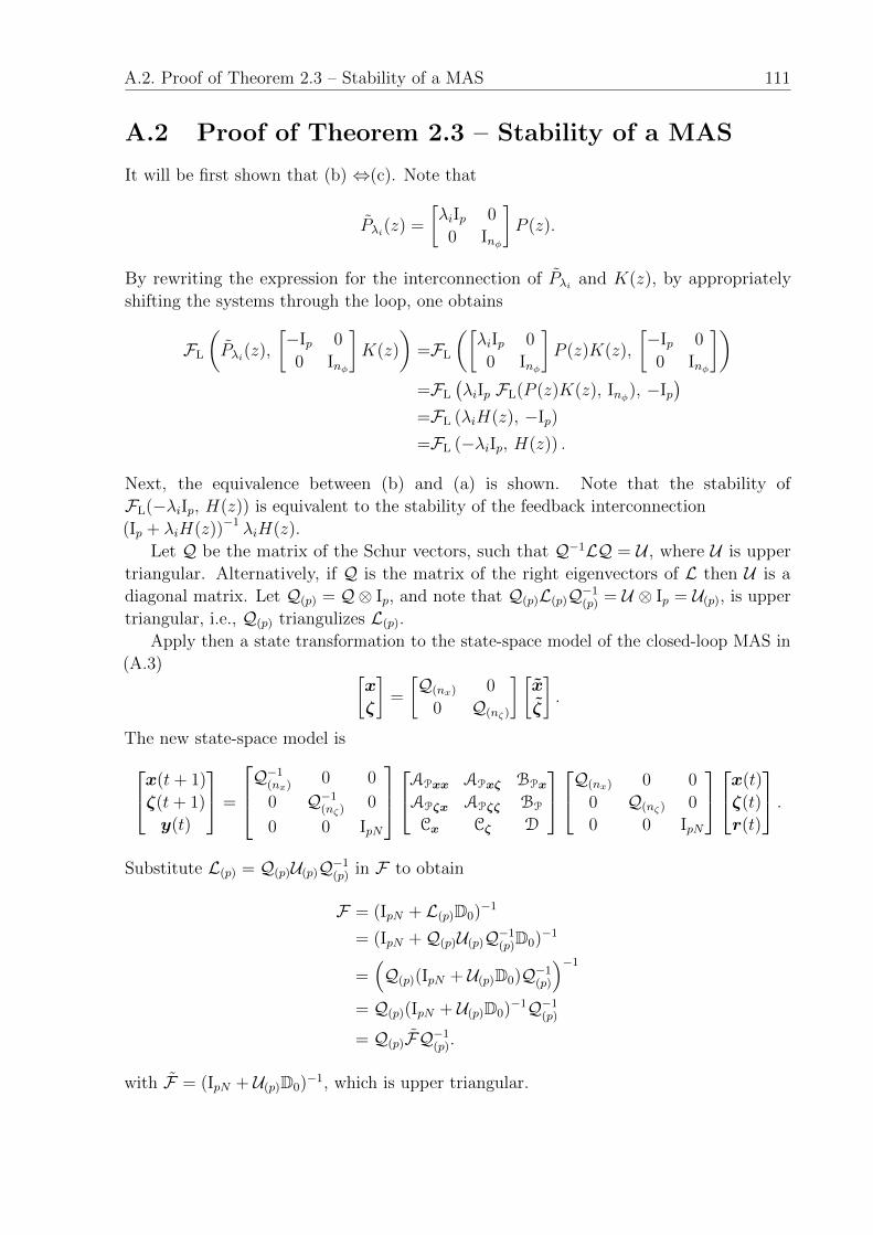
A.2. Proof of Theorem 2.3 – Stability of a MAS 111
A.2 Proof of Theorem 2.3 – Stability of a MAS
It will be first shown that (b) ⇔(c). Note that
Pλi(z) =
[λiIp 0
0 Inφ
]P (z).
By rewriting the expression for the interconnection of Pλi and K(z), by appropriately
shifting the systems through the loop, one obtains
FL
(Pλi(z),
[−Ip 0
0 Inφ
]K(z)
)=FL
([λiIp 0
0 Inφ
]P (z)K(z),
[−Ip 0
0 Inφ
])=FL
(λiIp FL(P (z)K(z), Inφ), −Ip
)=FL (λiH(z), −Ip)
=FL (−λiIp, H(z)) .
Next, the equivalence between (b) and (a) is shown. Note that the stability of
FL(−λiIp, H(z)) is equivalent to the stability of the feedback interconnection
(Ip + λiH(z))−1 λiH(z).
Let Q be the matrix of the Schur vectors, such that Q−1LQ = U , where U is upper
triangular. Alternatively, if Q is the matrix of the right eigenvectors of L then U is a
diagonal matrix. Let Q(p) = Q⊗ Ip, and note that Q(p)L(p)Q−1(p) = U ⊗ Ip = U(p), is upper
triangular, i.e., Q(p) triangulizes L(p).
Apply then a state transformation to the state-space model of the closed-loop MAS in
(A.3) [x
ζ
]=
[Q(nx) 0
0 Q(nζ)
] [x
ζ
].
The new state-space model isx(t+ 1)
ζ(t+ 1)
y(t)
=
Q−1(nx) 0 0
0 Q−1(nζ) 0
0 0 IpN
APxx APxζ BPx
APζx APζζ BP
Cx Cζ D
Q(nx) 0 0
0 Q(nζ) 0
0 0 IpN
x(t)
ζ(t)
r(t)
.Substitute L(p) = Q(p)U(p)Q−1
(p) in F to obtain
F = (IpN + L(p)D0)−1
= (IpN +Q(p)U(p)Q−1(p)D0)−1
=(Q(p)(IpN + U(p)D0)Q−1
(p)
)−1
= Q(p)(IpN + U(p)D0)−1Q−1(p)
= Q(p)FQ−1(p).
with F = (IpN + U(p)D0)−1, which is upper triangular.
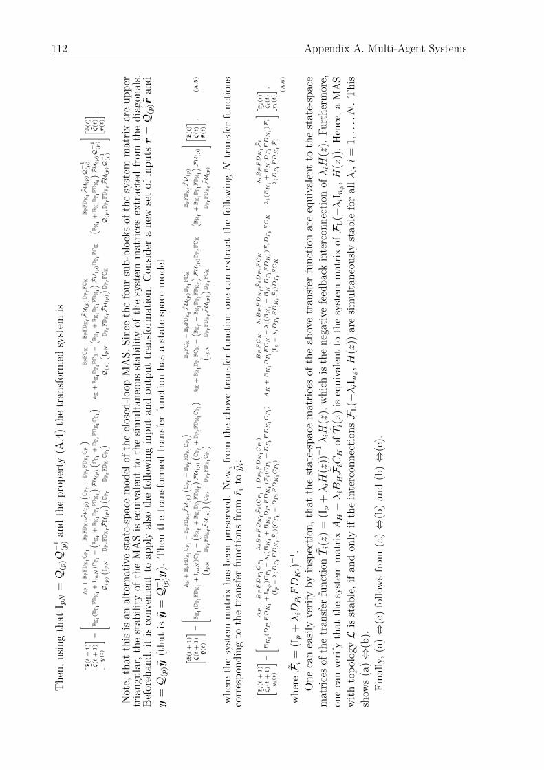
112 Appendix A. Multi-Agent SystemsT
hen
,usi
ng
that
I pN
=Q
(p)Q−
1(p
)an
dth
epro
per
ty(A
.4)
the
tran
sfor
med
syst
emis
x(t+
1)
ζ(t
+1)
y(t)
=
AP+
B PFD
KlCP l−
B PFD
KfFU(p)
( CP f
+DP f
FDKlCP l
)B P
FCK−
B PFD
KfFU(p)DP f
FCK
B PFD
KfFU(p)Q
−1
(p)
B Kl(D
P lFD
Kl+
I mN
)CP l−( B K
f+
B KlDP l
FDKf
) FU(p)
( CP f
+DP f
FDKlCP l
)AK
+B K
lDP l
FCK−( B K
f+
B KlDP l
FDKf
) FU(p)DP f
FCK
( B Kf+
B KlDP l
FDKf
) FU(p)Q
−1
(p)
Q(p)
( I pN−
DP f
FDKfFU(p)
)( CP f−
DP f
FDKlCP l
)Q
(p)
( I pN−
DP f
FDKfFU(p)
) DP f
FCK
Q(p)DP f
FDKfFU(p)Q
−1
(p)
x(t)
ζ(t)
r(t)
.
Not
e,th
atth
isis
anal
tern
ativ
est
ate-
spac
em
od
elof
the
clos
ed-l
oop
MA
S.
Sin
ceth
efo
ur
sub
-blo
cks
ofth
esy
stem
mat
rix
are
up
per
tria
ngu
lar,
the
stab
ilit
yof
the
MA
Sis
equiv
alen
tto
the
sim
ult
aneo
us
stab
ilit
yof
the
syst
emm
atri
ces
extr
acte
dfr
omth
edia
gonal
s.B
efor
ehan
d,
itis
conve
nie
nt
toap
ply
also
the
foll
owin
gin
pu
tan
dou
tpu
ttr
ansf
orm
atio
n.
Con
sid
era
new
set
ofin
pu
tsr
=Q
(p)r
and
y=Q
(p)y
(that
isy
=Q−
1(p
)y).
Then
the
tran
sfor
med
tran
sfer
funct
ion
has
ast
ate-
spac
em
odel
x(t+
1)
ζ(t
+1)
y(t)
=
AP+
B PFD
KlCP l−
B PFD
KfFU(p)
( CP f
+DP f
FDKlCP l
)B P
FCK−
B PFD
KfFU(p)DP f
FCK
B PFD
KfFU(p)
B Kl(D
P lFD
Kl+
I mN
)CP l−( B K
f+
B KlDP l
FDKf
) FU(p)
( CP f
+DP f
FDKlCP l
)AK
+B K
lDP l
FCK−( B K
f+
B KlDP l
FDKf
) FU(p)DP f
FCK
( B Kf+
B KlDP l
FDKf
) FU(p)
( I pN−
DP f
FDKfFU(p)
)( CP f−
DP f
FDKlCP l
)( I p
N−
DP f
FDKfFU(p)
) DP f
FCK
DP f
FDKfFU(p)
x(t)
ζ(t)
r(t)
,(A
.5)
wh
ere
the
syst
emm
atri
xh
asb
een
pre
serv
ed.
Now
,fr
omth
eab
ove
tran
sfer
fun
ctio
non
eca
nex
trac
tth
efo
llow
ingN
tran
sfer
fun
ctio
ns
corr
esp
ondin
gto
the
tran
sfer
funct
ions
from
r itoy i
:
x i(t
+1)
ζi(t
+1)
yi(t)
=
AP
+BPFDK
lCPl−λiBPFDK
fFi(CPf+DPfFDK
lCPl)
BPFCK−λiBPFDK
fFiDPfFCK
λiBPFDK
fFi
BK
l(DPlFDK
l+
I nφ)CPl−λi(BK
f+BK
lDPlFDK
f)Fi(CPf+DPfFDK
lCPl)
AK
+BK
lDPlFCK−λi(BK
f+BK
lDPlFDK
f)FiDPfFCK
λi(BK
f+BK
lDPlFDK
f)Fi
(Ip−λiDPfFDK
fFi)(CPf−DPfFDK
lCPl)
(Ip−λiDPfFDK
fFi)DPfFCK
λiDPfFDK
fFi
x i(t)
ζi(t)
ri(t)
, (A.6)
wher
eF i
=(Ip
+λiD
PfFDK
f)−
1.
On
eca
nea
sily
veri
fyby
insp
ecti
on,
that
the
stat
e-sp
ace
mat
rice
sof
the
abov
etr
ansf
erfu
nct
ion
are
equ
ival
ent
toth
est
ate-
spac
e
mat
rice
sof
the
tran
sfer
funct
ionTi(z)
=(Ip
+λiH
(z))−
1λiH
(z),
whic
his
the
neg
ativ
efe
edbac
kin
terc
onnec
tion
ofλiH
(z).
Furt
her
mor
e,
one
can
veri
fyth
atth
esy
stem
mat
rixAH−λiB
HF iCH
ofTi(z)
iseq
uiv
alen
tto
the
syst
emm
atri
xofF L
(−λiInφ,H
(z))
.H
ence
,a
MA
S
wit
hto
pol
ogyL
isst
able
,if
and
only
ifth
ein
terc
onnec
tion
sF L
(−λiInφ,H
(z))
are
sim
ult
aneo
usl
yst
able
for
allλi,i
=1,...,N
.T
his
show
s(a
)⇔
(b).
Fin
ally
,(a
)⇔
(c)
follow
sfr
om(a
)⇔
(b)
and
(b)⇔
(c).
Appendix B
Matrix Calculus
In order to derive several of the results in this work, some basic definitions and properties
of the gradients of function in matrix space are needed. Although many of the following
results are available elsewhere ([Skelton et al., 1998; Meyer, 2000; Petersen and Pedersen,
2008]) here they are provided for purposes of consistency and completeness, and since
certain simplifications due to the nature of the problems of interest can be applied.
B.1 Matrix Gradients
Definition B.1. The gradient (in matrix space) of a function f(X) : Rn×m → R w.r.t.
X is
∇Xf =∂f
∂X=
∂f∂X11
. . . ∂f∂X1m
.... . .
...∂f∂Xn1
. . . ∂f∂Xnm
. (B.1)
Definition B.2. The gradient (tangent) of a matrix valued function of a scalar F (x) :
R→ Rp×q is
∇xF =∂F
∂x=
∂F11
∂x. . . ∂F1q
∂x...
. . ....
∂Fp1∂x
. . . ∂Fpq∂x
. (B.2)
B.2 Chain Rule for Matrix Valued Functions
In the following it will be used, that for complex matrices A ∈ Cn×m and B ∈ Cm×n the
function f(A,B) = trace(A∗TB
), satisfies the properties of the inner product [Meyer,
2000] and hence one can write 〈A, B〉 = trace(A∗TB
). Recall that if X and Y are of
compatible dimensions then trace (XY ) =trace (Y X).
B.2.1 Real-Valued Functions of Real-Valued Variables
The chain rule for matrix functions (see, e.g., [Petersen and Pedersen, 2008]) is as follows.
Given the functions U(X) : Rn×m → Rp×q and f(U) : Rp×q → R, where U(X) ∈ Rp×q,
113
114 Appendix B. Matrix Calculus
X ∈ Rn×m, the partial derivative of f with respect to (w.r.t. ) element ik of X is
∂f
∂Xik
= trace
((∂f
∂U
)T∂U
∂Xik
)(B.3)
which using the ∇ notation can be written as
∇Xikf = trace(
(∇Uf )T∇XikU)
= 〈∇Uf , ∇XikU 〉 . (B.4)
Assume that ∇Uf is known and that U = AXB, where A ∈ Rp×n and B ∈ Rm×q. Then,
the gradient of U w.r.t. Xik is
∇XikU = AEikB, ∀i ∈ [1, n], ∀k ∈ [1,m], (B.5)
where Eik ∈ Rn×m is an elementary matrix, i.e., Eik = eieTk , where ei is column i of In and
ek is column k of Im.
Now one can rewrite
∇Xikf = 〈∇Uf , AEikB〉=trace
((∇Uf )TAEikB
)=trace
((∇Uf )TAeie
TkB)
=trace(
eTkB (∇Uf )TAei
)=eTkB (∇Uf )TAei.
Substituting in the elements of ∇Xf (see (B.1)) leads to
∇Xf =
eT1B (∇Uf )TAe1 . . . eTmB (∇Uf )TAe1...
. . ....
eT1B (∇Uf )TAen . . . eTmB (∇Uf )TAen
=(B (∇Uf )TA
)T,
where the last substitution is possible since eTi P ek in fact selects element Pik of P . Finally,
one obtains the gradient of f w.r.t. to X in matrix space as
∇Xf = AT∇Uf BT. (B.6)
The following simplified approach can be used to derive the desired gradients. Assume the
gradient of f(U(X, Y )) with respect to U(X, Y ) is known and the gradients of f(U(X, Y ))
with respect to X and Y are of interest. Let X be perturbed by a small value δX and Y
by a small value δY (i.e., matrices with much smaller norms than X and Y ), and assume
that U(X, Y ) = AXB + CYD. Then
U(X + δX , Y + δY ) = A(X + δX)B + C(Y + δY )D
= AXB + CYD + AδXB + CδYD
U(X + δX , Y + δY ) = U(X, Y ) + AδXB + CδYD. (B.7)
B.2. Chain Rule for Matrix Valued Functions 115
Now, by substituting δX = εEik, δY = 0 one can obtain the gradient
∇XikU = limε→0
U(X + εEik, Y )− U(X, Y )
ε= AEikB,
which is equivalent to the result in (B.5). From this, after following the above steps (and
after applying the same reasoning to Y ), the desired gradients can be obtained as
∇Xf = AT∇Uf BT, ∇Yf = CT∇Uf DT.
In the following these steps will be omitted, and as soon as an expression as in (B.7) is
obtained directly the resulting gradients will be stated.
Finally, recall that if f = f(P (X), Q(X)) where P (X) = AXB and Q(X) = CXD,
for A,B,C,D of appropriate dimensions, the total derivative of f w.r.t. X is the sum of
the corresponding partial derivatives, i.e.,
df
dXik
=∂f
∂Xik
+ trace
((∂f
∂P
)TdP
dXik
)+ trace
((∂f
∂Q
)TdQ
dXik
).
In the case when f is not directly dependent on X one can write
∇Xikf = 〈∇Pf , ∇XikP 〉+ 〈∇Qf , ∇XikQ 〉 ,
or finally for the gradient in matrix space one obtains
∇Xf =AT∇Pf BT + CT∇Qf DT.
B.2.2 Real-Valued Functions of Complex-Valued Variables
The following results on partial derivatives of functions of complex arguments and chain
rule are rigorously derived in [Brandwood, 1983] and presented in a compact form in
[Petersen and Pedersen, 2008]. They are provided here since in this work only real-valued
functions are of interest in which case some simplifications apply.
Lemma B.1 ([Brandwood, 1983]). Let g(u, u∗) : C× C→ C be a function of a complex
number u = x+ jy and its conjugate u∗ = x− jy, where x, y ∈ R. Let further g(u, u∗) =
f(x, y), where f(x, y) : R×R→ C. Then the partial derivatives are given by
∂g
∂u=
1
2
(∂f
∂x− j
∂f
∂y
), and
∂g
∂u∗=
1
2
(∂f
∂x+ j
∂f
∂y
).
For a function g(U,U∗) = f(U) of a complex matrix U = X + jY , where X, Y ∈ Rp×q,
the complex gradient operators are:
∇Ug =
∂g∂U11
. . . ∂g∂U1q
.... . .
...∂g∂Up1
. . . ∂g∂Upq
, ∇U∗g =
∂g∂U∗11
. . . ∂g∂U∗1q
.... . .
...∂g∂U∗p1
. . . ∂g∂U∗pq
. (B.8)
116 Appendix B. Matrix Calculus
For a real-valued function g(U(X), U∗(X)) : Cp×q × Cp×q → R, where X ∈ Rn×m and
U(X) : Rn×m → Cp×q, the complete derivative of g w.r.t. Xik can be obtained from
∇Xikg =trace(
(∇Ug )T∇XikU)
+ trace(
(∇U∗g )T∇XikU∗)
=trace(
(∇U∗g )∗T∇XikU + (∇U∗g )T∇XikU∗)
=Re{
2trace(
(∇U∗g )∗T∇XikU)}
=Re {〈2∇U∗g , ∇XikU 〉} ,
where it is used that ∇Ug = (∇U∗g )∗, since g is a real-valued function, and by noting that
the argument inside the trace is z + z∗ = 2Re {z}.Consequently, when U = AXB ∈ Cp×q, X ∈ Rn×m, and using that the gradient
g(U(X), U∗(X)) = f(U(X)) one obtains
∇Xf = Re{(B∗ (2∇U∗f )TA∗
)}T
= Re{A∗T2∇U∗f B∗T
}. (B.9)
Since it will be assumed that the functions of interest are analytic their gradients are
guaranteed to be real, so the real operator will be dropped and the factor 2 will be absorbed
into ∇U∗f , leading to the compact notation
∇Xf = A∗T∇Uf B∗T. (B.10)
Functions belonging to this class (real-valued functions of complex argument) are the
H∞ norm of a dynamic system, as function of the system matrices, as well as the spectral
radius of a matrix, as function of the entries of the matrix (as shown in Section 5.1.1).
Appendix C
Gradient Computations
In order to use the results from this appendix it is recommended, that one first accustoms
oneself with the notations and basic principles of gradient computation for matrix valued
functions provided in Appendix B.
C.1 Gradient of an Inverted Matrix
In order to find ∇AA−1 , i.e., the gradient of an inverse of a matrix w.r.t. to the matrix
elements, the following reformulation will be useful.
Given an invertible matrix X, add and subtract a second invertible matrix B as follows.
X−1 = X−1 +B−1 −B−1
= X−1BB−1 +B−1 −B−1
= X−1BB−1 +B−1 −X−1XB−1
= B−1 +X−1 (B −X)B−1
= B−1 −X−1 (X −B)B−1.
Now let an invertible matrix A be perturbed by a small perturbation matrix E. Then
substitute X = A+ E and B = A in the above equation to obtain:
(A+ E)−1 = A−1 −(A−1 + E
)−1(A+ E − A)A−1
= A−1 −(A−1 + E
)−1EA−1
= A−1 −(AE−1(A+ E)
)−1
= A−1 −(AE−1A+ A
)−1
= A−1 −((AE−1 + I
)A)−1
= A−1 − A−1(AE−1 + I
)−1
= A−1 − A−1((A+ E)E−1
)−1
= A−1 − A−1E(A+ E)−1,
which can be finally written as
(A+ E)−1 = A−1 − A−1EA−1 + o (E) , (C.1)
117
118 Appendix C. Gradient Computations
where o (E) denotes higher order terms of E. Then for a sufficiently small E (i.e., with
norm much smaller than the norm of A) one can write
(A+ E)−1 ≈ A−1 − A−1EA−1.
If A = A(X) ∈ Rn×m, where X ∈ Rp×q, and f(A) = A−1, then the gradient of f w.r.t.
Xik can be computed from
∇Xikf = −A−1 (∇XikA ) A−1. (C.2)
C.2 Gradient of the H∞ Norm w.r.t. the System
Matrices
The following derivation of the gradient of the H∞ norm of a system w.r.t. to the closed-
loop system matrices is the first step of the computation of the gradient of the H∞ norm
with respect to the controller matrices, i.e., the true decision variables. The computation of
the gradient of the H∞ norm w.r.t. the system matrix (i.e., ∇Af ) is presented in [Millstone,
2006], and the computation of all the gradients are implemented in hifoo [Burke et al.,
2006a; Gumussoy et al., 2009]. As these gradients are used in the gradient-based search
over controller and scaling by µ-synthesis in Section 5.2, and since the derivation of the
gradients w.r.t. the B, C and D matrices is not provided elsewhere, the gradients of the
closed-loop H∞ norm w.r.t. the system matrices are provided below.
Let M(z) =
A B
C D
be a state-space realization of a closed-loop, discrete-time LTI
system and let A has all its eigenvalues inside the unit disc (i.e., M(z) is stable transfer
functions). Let further the H∞ norm be attained at frequency ωx and
f = f(A,B,C,D) = ‖M(z)‖∞ = σ(Mx),
where Mx = CZ−1B + D and Z = ejωxIn − A. Let further u and v denote the left and
right singular vectors, corresponding to f = σ(Mx), i.e.,
u∗TMxv = f.
Then the gradient in matrix space of f w.r.t. the system matrices can be computed as
follows.
• (A) Assume that the system matrix A is perturbed by a matrix δA. For a small δAthe first-order Taylor series approximation gives:
f(A+ δA, B, C,D) = σ(C(Z − δA)−1B +D)
= σ(C(Z−1 + Z−1δAZ−1 + o (δA))B +D)
= σ(Mx + CZ−1δAZ−1B) + o (δA)
= σ(Mx) + u∗TCZ−1δAZ−1Bv + o (δA)
= f + trace(u∗TCZ−1δAZ
−1Bv)
+ o (δA)
= f + trace(Z−1Bvu∗TCZ−1δA
)+ o (δA)
= f +⟨(Z−1Bvu∗TCZ−1
)∗T, δA
⟩+ o (δA) ,
C.2. Gradient of the H∞ Norm w.r.t. the System Matrices 119
where the second line is obtained using (C.1). Hence the gradient in matrix space of
f w.r.t. A is
∇Af =(CZ−1
)∗Tuv∗T
(Z−1B
)∗T. (C.3)
• (B) Applying the same approach to the B matrix provides
f(A,B + δB, C,D) = σ(CZ−1(B + δB) +D)
= σ(Mx + CZ−1δB)
= σ(Mx) + u∗TCZ−1δBv + o (δB)
= f + trace(vu∗TCZ−1δB
)+ o (δB) ,
and finally the desired gradient is
∇Bf =(CZ−1
)∗Tuv∗T. (C.4)
• (C) By perturbing C one has
f(A,B,C + δC , D) = σ((C + δC)Z−1)B +D
= σ(MxδCZ−1B)
= σ(Mx) + u∗TδCZ−1Bv + o (δC)
= f + trace(Z−1Bvu∗TδC
)+ o (δC) ,
and hence
∇Cf = uv∗T(Z−1B)∗T. (C.5)
• (D) Similarly for D
f(A,B,C,D + δD) = σ(CZ−1B +D + δD)
= σ(Mx) + u∗TδDv + o (δD)
= f + trace(vu∗TδD
)+ o (δD) ,
so the gradient of f w.r.t. D is
∇Df = uv∗T. (C.6)
Note, that if Mx is a static gain, then in fact the gradient of f = σ(Mx) w.r.t. Mx is
∇Mxf = uv∗T. (C.7)
120 Appendix C. Gradient Computations
C.3 Subgradient of the H∞ Norm
The concept of subgradient or generalized derivative of a function has been introduced as
an approach in the non-smooth analysis for handling functions that are not differentiable
at every point (cf. [Clarke, 1990]). By the fixed-structure H∞ synthesis such points of
non-smoothness can occur, when the H∞ norm of the closed-loop system M(z) is attained
at a several frequencies simultaneously or/and when the maximal singular value has
multiplicity greater than one.
In the following, the concept of a subgradient and its relation to the gradient, and
in particular to the gradient of the closed-loop H∞ norm w.r.t. the system matrices, is
introduced in the form of an example. Consider a matrix Mx ∈ Cn×m, with a singular
value decomposition Mx = UΣV ∗T, and let the maximum singular value f = σ(Mx) has
a multiplicity of r, i.e., σ(Mx) = Σii, i = 1, . . . , r. Let ui and vi denote the ith singular
vectors of Mx, i.e., ui is column i of U and vi is column i of V . Then one can write the
following
f = σ(Mx) = u∗Ti Mxvi, i = 1, . . . , r.
Recall, that according (C.7) all of the expressions
∇Mxf = uiv∗Ti , i = 1, . . . , r, (C.8)
hold. These are called a subgradients of f = σ(Mx) w.r.t. Mx. In fact, any convex
combination of such subgradients will be again a subgradient of f w.r.t. Mx. Then one
needs to select among these subgradients one (e.g., corresponding to the steepest descent
direction) and use it to update the decision variables. However, since uiv∗Tk 6= 0, for
i 6= k it is difficult to express the problem of choosing a descent direction conveniently as
an optimization problem. However, by rewriting v∗Ti = u∗Ti Mx/σ(Mx), i = 1, . . . , r and
substituting in (C.8) one obtains
∇Mxf = uiu∗Ti Mx
1
σ(Mx), i = 1, . . . , r. (C.9)
Let
Ur =[u1 . . . ur
].
Then one can write the generalized gradient of f w.r.t. Mx, i.e., the set of all subgradients
of f w.r.t. Mx as
∇Mxf = UrY U∗Tr Mx
1
σ(Mx), (C.10)
where Y ∈ Cr×r, s.t., Y � 0, trace (Y ) = 1. Indeed, since uiu∗Tk = 0, ∀i 6= k (due to U
being unitary) only the sum of the diagonal elements of Y needs to be one in order to
provide a convex combination of the term in (C.9). The same approach can by applied to
(C.3)–(C.6) to obtain the generalized gradients of f w.r.t. the system matrices of M(z).
In [Apkarian and Noll, 2006b] the following approach is used for computing the
subgradient
g = arg minY‖∇Mxf‖, (C.11)
C.4. Gradient Computation by Optimization over Controller and Scalings 121
needed for obtaining the steepest descent direction d = − g‖g‖ . Let X ∈ Cmn×r2 be such
that
vec (∇Mxf) = Xvec(Y ) = Xy,
where for a matrix vec(•) denotes the vector of the stacked columns, i.e.,
y = vec(Y ) =[Y11 Y21 . . . Yr1 Y12 Y22 . . . Yrr
]T.
Details on the construction of such X can be found in [Popov, 2010]. Now the problem in
(C.11) can be expressed as the following LMI problem (see [Apkarian and Noll, 2006b])
minimize ϑ
subject to
[ϑ •Xy ϑImn
]� 0, Y � 0, trace (Y ) = 1.
The last constraint, trace (Y ) = 1, can be alternatively expressed as 1Tr2y = 1, where
1r2 ∈ Rr2 is a vector each element of which is equal to one. This LMI problem can be solved
for ϑ and y = vec(Y ), and the direction of steepest descent computed as d = −Xy/‖Xy‖.
C.4 Gradient Computation by Optimization over
Controller and Scalings
C.4.1 Static Scalings
Using the simplified approach introduced in Appendix B.2, assume that the matrices in
(5.8), i.e., D, A, B1, . . . , D22 are perturbed by matrices δD, δAM , δB1 , . . . , δD22 with a much
smaller norm. Then, as AQ depends only on AM one obtains
AQ(AM + δAM ) = AM + δAM = AQ + δAM ,
from which it is clear that the gradient of f w.r.t. AM is ∇AMf = ∇AQf . Similarly,
∇B2f = ∇BQ,2f , ∇C2f = ∇CQ,2f and ∇D2,2f = ∇DQ,22f .
The remaining perturbed matrices are obtained as follows.
BQ,1(B1 + δB1 , D + δD) = (B1 + δB1)(D + δD)−1
which using the result for an inverse of a matrix from Appendix C.1 leads to
BQ,1(B1 + δB1 , D + δD) = (B1 + δB1)(D−1 −D−1δDD−1 + o (D))
≈ B1D−1 + δB1D−1 −B1D−1δDD−1 + o (δB1 , δD)
≈ BQ,1 + δB1D−1 −B1D−1δDD−1
and, similarly
CQ,1(C1 + δC1 , D + δD) = (D + δD)(C1 + δC1)
≈ CQ,1 + δDC1 + DδC1
DQ,11(D11 + δD11 , D + δD) = (D + δD)(D11 + δD11)(D + δD)−1
≈ DQ,11 + δDD11D−1 + DδD11D−1 −DD11D−1δDD−1,
122 Appendix C. Gradient Computations
where o (•) represents higher order terms depending on •, which are neglected. The result
for DQ,21 is analogous to the result for BQ,1 (i.e., simply exchange B1 with D21) and the
result for DQ,12 is analogous to the result for CQ,1.
Then, by applying the chain rule (see Appendix B.2), and summing the corresponding
terms in the case of D one obtains the required gradients:
∇AMf = ∇AQf ,
∇BMf =[∇BQ,1f D−T ∇BQ,2f
]= ∇Bf Q
[D−1 0
0 Inv
]T,
∇CMf =
[DT∇CQ,1f∇CQ,2f
]=
[D 0
0 Inw
]T∇CQf ,
∇DMf =
[DT∇DQ,11f D−T DT∇DQ,12f∇DQ,21f D−T ∇DQ,22f
]=
[D 0
0 Inw
]T∇DQf
[D−1 0
0 Inv
]T,
∇Df = −(B1D−1)T∇BQ,1f D−T +∇CQ,1f CT1
− (D21D−1)T∇DQ,21f D−T +∇DQ,12f DT12
+∇DQ,11f (D11D−1)T − (DD11D−1)T∇DQ,11f D−T.
C.4.2 Gradient w.r.t. Dynamic Scalings
Using the same principle of variations as in Appendix C.4.1 one directly obtains equations
(5.17)–(5.28). In order to obtain equations (5.29)–(5.32) one needs to apply the same
approach to the state-matrixes of DJ(s):
AJ(AL + δAL , . . . , DL + δDL) =AJ + δAL − δBLD−1L CL
+BLD−1L δDLD
−1L CL −BLD
−1L δCL + o (•)
BJ(BL + δBL , DL + δDL) =BJ + δBLD−1L −BLD
−1L δDLD
−1L + o (•)
CJ(CL + δCL , DL + δDL) =CJ +D−1L δDLD
−1L CL −D−1
L δCL + o (•)DJ(DL + δDL) =DJ −D−1
L δDLD−1L .
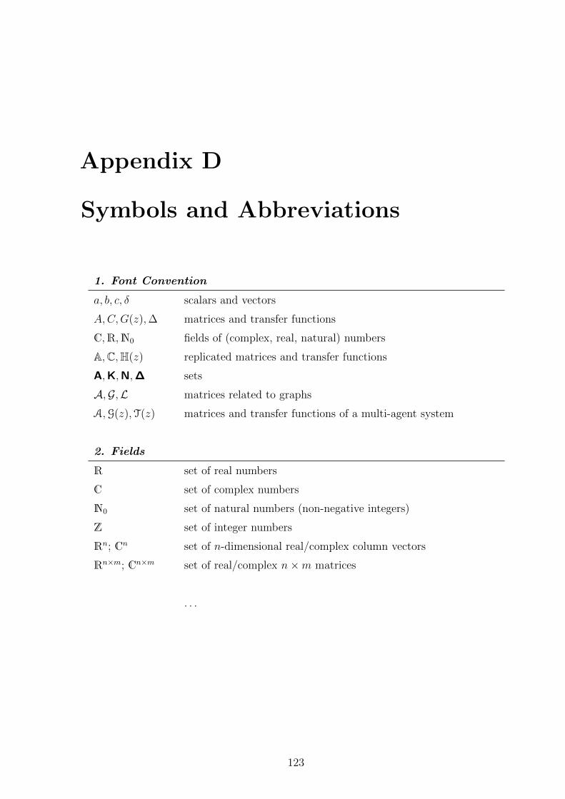
Appendix D
Symbols and Abbreviations
1. Font Convention
a, b, c, δ scalars and vectors
A,C,G(z),∆ matrices and transfer functions
C,R,N0 fields of (complex, real, natural) numbers
A,C,H(z) replicated matrices and transfer functions
A,K,N,∆ sets
A,G,L matrices related to graphs
A,G(z),T(z) matrices and transfer functions of a multi-agent system
2. Fields
R set of real numbers
C set of complex numbers
N0 set of natural numbers (non-negative integers)
Z set of integer numbers
Rn; Cn set of n-dimensional real/complex column vectors
Rn×m; Cn×m set of real/complex n×m matrices
. . .
123
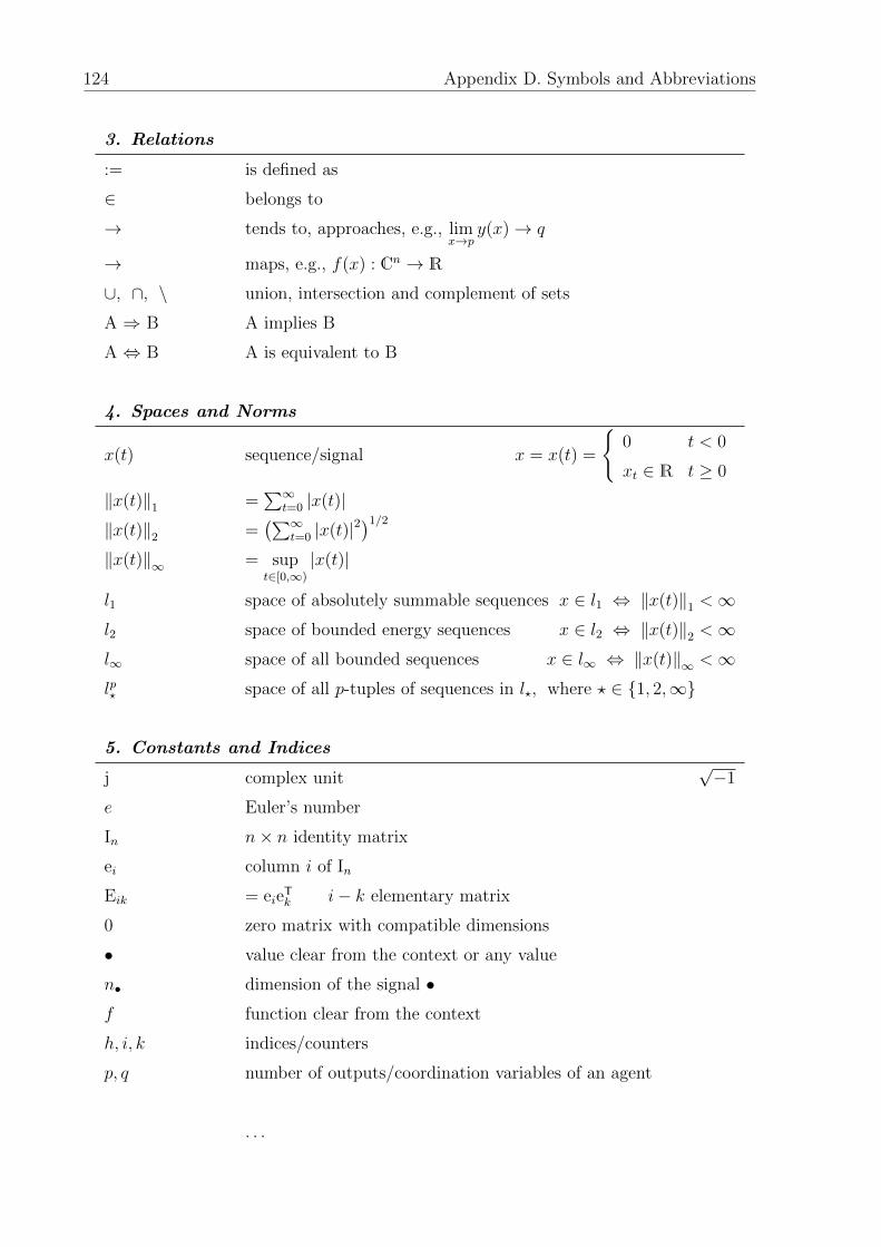
124 Appendix D. Symbols and Abbreviations
3. Relations
:= is defined as
∈ belongs to
→ tends to, approaches, e.g., limx→p
y(x)→ q
→ maps, e.g., f(x) : Cn → R
∪, ∩, \ union, intersection and complement of sets
A ⇒ B A implies B
A ⇔ B A is equivalent to B
4. Spaces and Norms
x(t) sequence/signal x = x(t) =
{0 t < 0
xt ∈ R t ≥ 0
‖x(t)‖1 =∑∞
t=0 |x(t)|‖x(t)‖2 =
(∑∞t=0 |x(t)|2
)1/2
‖x(t)‖∞ = supt∈[0,∞)
|x(t)|
l1 space of absolutely summable sequences x ∈ l1 ⇔ ‖x(t)‖1 <∞l2 space of bounded energy sequences x ∈ l2 ⇔ ‖x(t)‖2 <∞l∞ space of all bounded sequences x ∈ l∞ ⇔ ‖x(t)‖∞ <∞lp? space of all p-tuples of sequences in l?, where ? ∈ {1, 2,∞}
5. Constants and Indices
j complex unit√−1
e Euler’s number
In n× n identity matrix
ei column i of In
Eik = eieTk i− k elementary matrix
0 zero matrix with compatible dimensions
• value clear from the context or any value
n• dimension of the signal •f function clear from the context
h, i, k indices/counters
p, q number of outputs/coordination variables of an agent
. . .
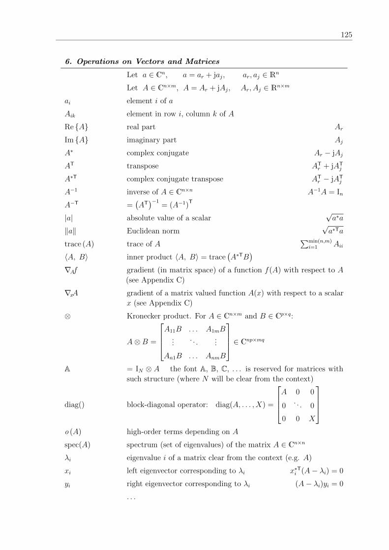
125
6. Operations on Vectors and Matrices
Let a ∈ Cn, a = ar + jaj, ar, aj ∈ Rn
Let A ∈ Cn×m, A = Ar + jAj, Ar, Aj ∈ Rn×m
ai element i of a
Aik element in row i, column k of A
Re {A} real part Ar
Im {A} imaginary part Aj
A∗ complex conjugate Ar − jAj
AT transpose ATr + jAT
j
A∗T complex conjugate transpose ATr − jAT
j
A−1 inverse of A ∈ Cn×n A−1A = In
A−T =(AT)−1
= (A−1)T
|a| absolute value of a scalar√a∗a
‖a‖ Euclidean norm√a∗Ta
trace (A) trace of A∑min(n,m)
i=1 Aii
〈A, B〉 inner product 〈A, B〉 = trace(A∗TB
)∇Af gradient (in matrix space) of a function f(A) with respect to A
(see Appendix C)
∇xA gradient of a matrix valued function A(x) with respect to a scalar
x (see Appendix C)
⊗ Kronecker product. For A ∈ Cn×m and B ∈ Cp×q:
A⊗B =
A11B . . . A1mB
.... . .
...
An1B . . . AnmB
∈ Cnp×mqA = IN ⊗ A the font A, B, C, . . . is reserved for matrices with
such structure (where N will be clear from the context)
diag() block-diagonal operator: diag(A, . . . , X) =
A 0 0
0. . . 0
0 0 X
o (A) high-order terms depending on A
spec(A) spectrum (set of eigenvalues) of the matrix A ∈ Cn×n
λi eigenvalue i of a matrix clear from the context (e.g. A)
xi left eigenvector corresponding to λi x∗Ti (A− λi) = 0
yi right eigenvector corresponding to λi (A− λi)yi = 0
. . .
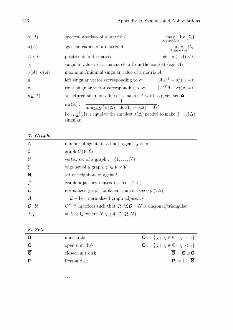
126 Appendix D. Symbols and Abbreviations
α (A) spectral abscissa of a matrix A maxλi∈spec(A)
Re {λi}
ρ (A) spectral radius of a matrix A maxλi∈spec(A)
|λi|
A � 0 positive definite matrix ⇔ α (−A) < 0
σi singular value i of a matrix clear from the context (e.g. A)
σ(A); σ(A) maximum/minimal singular value of a matrix A
ui left singular vector corresponding to σi (AA∗T − σ2i )ui = 0
vi right singular vector corresponding to σi (A∗TA− σ2i )vi = 0
µ∆(A) structured singular value of a matrix A w.r.t. a given set ∆
µ∆(A) :=1
min∆∈∆ { σ(∆) | det(In − A∆) = 0} ,
i.e., µ−1∆ (A) is equal to the smallest σ(∆) needed to make (In−A∆)
singular.
7. Graphs
N number of agents in a multi-agent system
G graph G (V, E)V vertex set of a graph := {1, . . . , N}E edge set of a graph, E ∈ V × VNi set of neighbors of agent i
J graph adjacency matrix (see eq. (2.4))
L normalized graph Laplacian matrix (see eq. (2.5))
A = L − IN normalized graph adjacency
Q, U CN×N matrices such that Q−1LQ = U is diagonal/triangular
X(•) = X ⊗ I•, where X ∈ {A, L, Q, U}
8. Sets
O unit circle O := {χ | χ ∈ C, |χ| = 1}Θ open unit disk Θ := {χ | χ ∈ C, |χ| < 1}Θ closed unit disk Θ = Θ ∪O
P Perron disk P := 1 + Θ
. . .
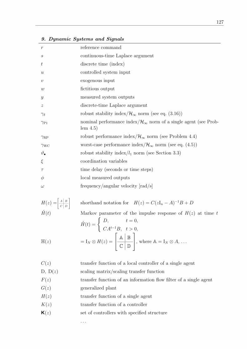
127
9. Dynamic Systems and Signals
r reference command
s continuous-time Laplace argument
t discrete time (index)
u controlled system input
v exogenous input
w fictitious output
y measured system outputs
z discrete-time Laplace argument
γδ robust stability index/H∞ norm (see eq. (3.16))
γP1 nominal performance index/H∞ norm of a single agent (see Prob-
lem 4.5)
γRP robust performance index/H∞ norm (see Problem 4.4)
γWC worst-case performance index/H∞ norm (see eq. (4.5))
ϑ• robust stability index/l1 norm (see Section 3.3)
ξ coordination variables
τ time delay (seconds or time steps)
φ local measured outputs
ω frequency/angular velocity [rad/s]
H(z) = A B
C D
shorthand notation for H(z) = C(zIn − A)−1B +D
H(t) Markov parameter of the impulse response of H(z) at time t
H(t) =
{D, t = 0,
CAt−1B, t > 0,
H(z) = IN ⊗H(z) =
A B
C D
, where A = IN ⊗ A, . . .
C(z) transfer function of a local controller of a single agent
D, D(z) scaling matrix/scaling transfer function
F (z) transfer function of an information flow filter of a single agent
G(z) generalized plant
H(z) transfer function of a single agent
K(z) transfer function of a controller
K(z) set of controllers with specified structure
. . .
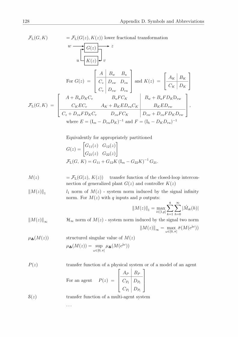
128 Appendix D. Symbols and Abbreviations
FL(G,K) = FL(G(z), K(z)) lower fractional transformation
G(z)
K(z)
zw
vu
For G(z) =
A Bw Bu
Cz Dzw Dzu
Cv Dvw Dvu
and K(z) =
AK BK
CK DK
FL(G,K) =
A+BuDKCv BuFCK Bw +BuFDKDvw
CKECv AK +BKEDvuCK BKEDvw
Cz +DzuFDKCv DzuFCK Dzw +DzuFDKDvw
,where E = (Im −DvuDK)−1 and F = (Ih −DKDvu)
−1
Equivalently for appropriately partitioned
G(z) =
[G11(z) G12(z)
G21(z) G22(z)
]FL(G, K) = G11 +G12K (Im −G22K)−1G21.
M(z) = FL(G(z), K(z)) transfer function of the closed-loop intercon-
nection of generalized plant G(z) and controller K(z)
‖M(z)‖1 l1 norm of M(z) - system norm induced by the signal infinity
norm. For M(z) with q inputs and p outputs:
‖M(z)‖1 = maxi∈[1,p]
q∑k=1
∞∑h=0
|Mik(h)|
‖M(z)‖∞ H∞ norm of M(z) - system norm induced by the signal two norm
‖M(z)‖∞ = maxω∈[0, π]
σ(M(ejω))
µ∆(M(z)) structured singular value of M(z)
µ∆(M(z)) = supω∈[0, π]
µ∆(M(ejω))
P (z) transfer function of a physical system or of a model of an agent
For an agent P (z) =
AP BP
CPfDPf
CPlDPl
S(z) transfer function of a multi-agent system
. . .
129
T (z) = (Ip +H(z))−1H(z) generalized plant interconnection of a single
agent for the purpose of robust stability analysis
TA(z) = A⊗ T (z) (see eq. (3.1))
V•(z), W•(z) transfer function of a shaping filter •Y (z) = FL(P (z)K(z), Im) closed-loop of vehicle and controller
∆; ∆(z) uncertain gain matrix
∆ set of uncertain matrices with a specified structure
Ψ(z) controller containing both F (z) and C(z) of both cooperation and
consensus modules
10. Abbreviations
BMI Bilinear Matrix Inequality
DoF Degree of Freedom
DOI Digital Object Identifier (cf. http://dx.doi.org)
GPS Global Positioning System
IMU Inertial Measurement Unit
LFT Linear Fractional Transformation
LMI Linear Matrix Inequality
LTI Linear Time Invariant
MAS Multi-Agent System
MIMO Multiple Inputs – Multiple Outputs
NP Nominal Performance
RP Robust Performance
RS Robust Stability
SISO Single Input – Single Output
SSV Structured Singular Value
UAV Unmanned Aerial Vehicle
UUV Unmanned Underwater Vehicle
WC Worst Case
w.r.t. with respect to

This page is intentionally left blank for pagination.
Bibliography
Abbas, H., Chughtai, S. and Werner, H. (2008). A hybrid gradient-LMI algorithm
for solving BMIs in control design problems. In Proc. 17th IFAC World Congress , pages
14319–14323. Seoul, South Korea, DOI: 10.3182/20080706-5-KR-1001.02426.
Ali, M., Abbas, H. and Werner, H. (2010). Controller synthesis for input-output lpv
models. In Proc. 49th IEEE Conference on Decision and Control , pages 7694–7699.
ISSN 0743-1546, DOI: 10.1109/CDC.2010.5717576.
Anderson, B., Yu, C., Fidan, B. and Hendrickx, J. (2008). Rigid graph control
architectures for autonomous formations. IEEE Control Systems Magazine 28(6), 48–63.
ISSN 0272-1708, DOI: 10.1109/MCS.2008.929280.
Apkairan, P. and Adams, R. (2000). Advanced gain-scheduling techniques for uncertain
systems, In L. Ghaoui and S. Niculescu, eds., Advances in Linear Matrix Inequality
Methods in Control . Advances in Design and Control. Philadelphia, PA, USA: SIAM.
ISBN 97808987143388, pages 209–228.
Apkarian, P. (2010). Nonsmooth µ-synthesis. International Journal of Robust and
Nonlinear Control online, DOI: 10.1002/rnc.1644.
Apkarian, P. and Noll, D. (2006a). Controller design via nonsmooth multidi-
rectional search. SIAM Journal in Control and Optimization 44(6), 1923–1949,
DOI: 10.1137/S0363012904441684.
Apkarian, P. and Noll, D. (2006b). Nonsmooth H∞ synthesis. IEEE Transactions on
Automatic Control 51(1), 71–86, DOI: 10.1109/TAC.2005.860290.
Astrom, K. and Wittenmark, B. (1997). Computer-Controlled Systems: theory and
design. Upper Saddle River, NJ: Prentice-Hall, 3rd edition. ISBN 978-0133148992.
Balas, G., Doyle, J., Glover, K., Packard, A. and Smith, R. (2001). µ-Analysis
and Synthesis Toolbox . The MathWorks.
Balch, T. and Arkin, R. (1998). Behavior-based formation control for multirobot
teams. IEEE Transactions on Robotics and Automation 14(6), 926–939. ISSN 1042-
296X, DOI: 10.1109/70.736776.
Borrelli, F. and Keviczky, T. (2006). Distributed LQR design for dynamically decou-
pled systems. In Proc. 45th IEEE Conference on Decision and Control , pages 5639–5644.
San Diego, CA, USA, DOI: 10.1109/CDC.2006.377294.
131
132 BIBLIOGRAPHY
Boyd, S. and Doyle, J. (1987). Comparison of peak and RMS gains for discrete-time
systems. Systems & Control Letters 9(1), 1–6. ISSN 0167-6911, DOI: 10.1016/0167-
6911(87)90002-8.
Boyd, S. and Vandenberghe, L. (2004). Convex Optimization. Cambridge University
Press. ISBN 0-521-83378-7.
Braatz, R. P., Young, P. M., Doyle, J. C. and Morari, M. (1994). Computational
complexity of calculation. IEEE Transactions on Automatic Control 39(5), 1000–1002,
DOI: 10.1109/9.284879.
Brandwood, D. (1983). A complex gradient operator and its application in adaptive
array theory. IEE Proceedings-F: Communications, Radar and Signal Processing 130(1),
11–16. ISSN 0143-7070, DOI: 10.1049/ip-f-1:19830003.
Brewer, J. W. (1978). Kronecker products and matrix calculus in system the-
ory. IEEE Transactions on Circuits and Systems 25(9), 772–781. ISSN 0098-4094,
DOI: 10.1109/TCS.1978.1084534.
Bruinsma, N. A. and Steinbuch, M. (1990). A fast algorithm to compute the H∞-norm of a transfer function matrix. Systems & Control Letters 14(4), 287–293. ISSN
0167-6911, DOI: 10.1016/0167-6911(90)90049-Z.
Bullo, F., Cortes, J. and Martınez, S. (2008). Distributed Control of Robotic
Networks. Applied Mathematics Series. Princeton University Press, Online: http:
//coordinationbook.info. Manuscript under contract.
Bunday, B. D. (1985). Basic Optimisation Methods. Arnold, London. ISBN 978-
0713135060.
Burke, J., Henrion, D., Lewis, A. and Overton, M. (2006a). hifoo - a Matlab
package for fixed-order controller design and H∞ optimization. In IFAC Symposium on
Robust Control Design. Toulouse, France, DOI: 10.3182/20060705-3-FR-2907.00059.
Burke, J., Henrion, D., Lewis, A. and Overton, M. (2006b). Stabilization via
nonsmooth, nonconvex optimization. IEEE Transactions on Automatic Control 51(11),
1760–1769. ISSN 0018-9286, DOI: 10.1109/TAC.2006.884944.
Burke, J., Lewis, A. and Overton, M. (2003). A nonsmooth, nonconvex optimization
approach to robust stabilization by static output feedback and low-order controllers. In
Proc. IFAC Symposium on Robust Control Design. Milan, Italy.
Castillo, P., Lozano, R. and Dzul, A. E. (2005). Modelling and Control of Mini-
Flying Machines. Advances in Industrial Control. Springer. ISBN 978-1-85233-957-9,
DOI: 10.1007/1-84628-179-2.
Caughman, J., Lafferriere, G., Veerman, J. and Williams, A. (2005). Decen-
tralized control of vehicle formations. Systems & Control Letters 54(9), 899–910,
DOI: 10.1016/j.sysconle.2005.02.004.

BIBLIOGRAPHY 133
Chopra, N. and Spong, M. (2006). Output synchronization of nonlinear systems with
time delay in communication. In Proc. 45th IEEE Conference on Decision and Control ,
pages 4986–4992. San Diego, CA, USA, DOI: 10.1109/CDC.2006.377258.
Chopra, N., Stipanovic, D. and Spong, M. (2008). On synchronization and collision
avoidance for mechanical systems. In Proc. American Control Conference, pages 3713–
3718. Seattle, WA, USA, DOI: 10.1109/ACC.2008.4587071.
Clarke, F. H. (1990). Optimization and Nonsmooth Analysis. Philadelphia, PA, USA:
SIAM. ISBN 978-0-898712-56-8.
Cortes, J., Martınez, S., Karatas, T. and Bullo, F. (2004). Coverage control
for mobile sensing networks. IEEE Transactions on Robotics and Automation 20(2),
243–255, DOI: 10.1109/TRA.2004.824698.
Dahleh, M. A. and Khammash, M. H. (1993). Controller design for plants with
structured uncertainty. Automatica 29(1), 37–56. ISSN 0005-1098, DOI: 10.1016/0005-
1098(93)90173-Q.
Dahleh, M. A. and Ohta, Y. (1988). A necessary and sufficient condition for ro-
bust BIBO stability. Systems & Control Letters 11(4), 271–275. ISSN 0167-6911,
DOI: 10.1016/0167-6911(88)90070-9.
Dailey, R. L. (1991). H∞ and µ methods for robust control. Workshop Lecture Notes,
30th IEEE Conference on Decision and Control.
D’Oliveira, M., Geromel, J. and Bernussou, J. (1999). An LMI optimization
approach to multiobjective controller design for discrete-time systems. In Proc. 38th
IEEE Conference on Decision and Control , pages 3611–1616. Phoenix, AZ , USA,
DOI: 10.1109/CDC.1999.827913.
Doyle, J. C. (1985). Structured uncertainty in control system design. In Proc. 24th
IEEE Conference on Decision and Control , pages 260–265. Fort Lauderdale, FL, USA,
DOI: 10.1109/CDC.1985.268842.
Dunbar, W. and Murray, R. (2002). Model predictive control of coordinated multi-
vehicle formations. In Proc. 41st IEEE Conference on Decision and Control , pages
4631–4636. Las Vegas, NV, USA. ISSN 0191-2216, DOI: 10.1109/CDC.2002.1185108.
Farag, A. and Werner, H. (2005). Fixed-order control of active suspension: a hybrid
evolutionary-algebraic approach. In Proc. 16th IFAC World Congress , pages 171–176.
Prague, Czech Republic, DOI: 10.3182/20050703-6-CZ-1902.00428.
Fax, J. A. (2002). Optimal and cooperative control of vehicle formations . Ph.D. thesis, Cal-
ifornia Institute of Technology, Online: http://resolver.caltech.edu/CaltechETD:
etd-10242005-105000.
Fax, J. A. and Murray, R. M. (2004). Information flow and cooperative control
of vehicle formations. IEEE Journal on Automatic Control 49(9), 1465–1476. ISSN
0018-9286, DOI: 10.1109/TAC.2004.834433.
134 BIBLIOGRAPHY
Frost and Sullivan, L. (2008). Study analysing the current activities in the field
of UAV. Contract notice ENTR/07/065 2008/S 1-000069, European Commission,
Online: http://ec.europa.eu/enterprise/policies/security/files/uav_study_
element_2_en.pdf.
Ghaoui, L. E. and Balakrishnan, V. (1994). Synthesis of fixed structure controllers
via numerical optimization. In Proc. 33rd IEEE Conference on Decision and Control ,
pages 2678–2683. Lake Buena Vista, FL, USA, DOI: 10.1109/CDC.1994.411398.
Glover, F. and Kochenberger, G., eds. (2003). Handook of Metaheuristics. In-
ternational Series in Operation Research & Management Science. Kluwer Academic
Publisher.
Goh, K., Turan, L., Safonov, M., Papavassiloupoulos, G. and Ly, J. (1994). Bi-
affine matrix inequality properties and computational methods. In Proc. American Con-
trol Conference, pages 850–855. Baltimore, MD, USA, DOI: 10.1109/ACC.1994.751863.
Gonzalez, T., ed. (2007). Handbook of Approximation Algorithms and Metaheuristics.
Chapman & Hall/CRC. ISBN 1584885505.
Gu, D. (2008). A differential game approach to formation control. IEEE
Transactions on Control Systems Technology 16(1), 85–93. ISSN 1063-6536,
DOI: 10.1109/TCST.2007.899732.
Gumussoy, S., Henrion, D., Millstone, M. and Overton, M. (2009). Multiobjective
robust control with hifoo 2.0. In Proc. IFAC Symposium on Robust Control Design.
Haifa, Israel, DOI: 10.3182/20090616-3-IL-2002.00025.
Gumussoy, S., Millstone, M. and Overton, M. (2008). H∞ strong stabilization via
hifoo, a package for fixed-order controller design. In Proc. 47th IEEE Conference on De-
cision and Control , pages 4135–4140. Cancun, Mexico, DOI: 10.1109/CDC.2008.4738750.
Gumussoy, S. and Overton, M. (2008). Fixed-order H∞ controller design via hifoo,
a specialized nonsmooth optimization package. In Proc. American Control Conference,
pages 2750–2754. Seattle, WA, USA. ISSN 0743-1619, DOI: 10.1109/ACC.2008.4586909.
Han, B., Overton, M. and Yu, T. (2003). Design of hermite subdivision schemes
aided by spectral radius optimzation. SIAM Journal on Scientific Computing 25(2),
643–656, DOI: 10.1137/S1064827502408608.
He, Y. and Wang, Q. (2006). An improved ILMI method for static output feedback
control with application to multivariable PID controller. IEEE Transaction on Automatic
Control 51(10), 1678–1683, DOI: 10.1109/TAC.2006.883029.
Henrion, D. (2005). LMI optimization for fixed-order H∞ controller design, In Positive
Polynomials in Control , volume 312 of Lecture Notes in Control and Information
Sciences . Springer Berlin/Heidelberg, pages 73–85, DOI: 10.1007/10997703.
BIBLIOGRAPHY 135
Henrion, D., Lofberg, J., Kocvara, M. and Stingl, M. (2005). Solving polynomial
static output feedback problems with PENBMI. In Proc. 44th IEEE Conference on
Decision and Control , pages 7581–7586. Seville, Spain, DOI: 10.1109/CDC.2005.1583385.
Henrion, D., Sebek, M. and Kucera, V. (2003). Positive polynomials and robust
stabilization with fixed-order controllers. IEEE Transactions on Automatic Control
48(7), 1178–1186, DOI: 10.1109/TAC.2003.814103.
Hirche, S. and Hara, S. (2008). Stabilizing interconnection characterization for multi-
agent systems with dissipative properties. In Proc. 17th IFAC World Congress , pages
1571–1577. Seoul, South Korea, DOI: 10.3182/20080706-5-KR-1001.1696.
Hol, C., Scherer, C., van der Meche, E. and Bosgra, O. (2003). A trust-region
interior point approach to fixed-order control applied to the benchmark system. In Proc.
International Workshop: Design and Optimisation of Restricted Complexity Controllers ,
pages 1–6. Grenoble, France.
Horn, R. and Johnson, C. (1985). Matrix Analysis . Cambridge: Cambridge University
press. ISBN 0521305861.
Iwasaki, T. (1997). Robust stability analysis with quadratic separator: parametric
time-varying uncertainty case. In Proc. 36th IEEE Conference on Decision and Control ,
pages 4880–4885. San Diego, CA, USA, DOI: 10.1109/CDC.1997.649805.
Jadbabaie, A., Lin, J. and Morse, A. (2003). Coordination of groups of mobile
autonomous agents using nearest neighbor rules. IEEE Transactions on Automatic
Control 48(6), 988–1001, DOI: 10.1109/TAC.2003.812781.
Kao, C.-Y. and Rantzer, A. (2005). Robust stability analysis of linear systems with
time-varying delays. In Proc. 16th IFAC World Congress , pages 173–178. Prague, Czech
Republic, DOI: 10.3182/20050703-6-CZ-1902.00973.
Keviczky, T., Borrelli, F., Fregene, K., Godbole, D. and Balas, G. (2008). De-
centralized receding horizon control and coordination of autonomous vehicle formations.
IEEE Transactions on Control Systems Technology 16(1), 19–33. ISSN 1063-6536,
DOI: 10.1109/TCST.2007.903066.
Khammash, M. and Pearson, J.B., J. (1991). Performance robustness of discrete-time
systems with structured uncertainty. IEEE Transactions on Automatic Control 36(4),
398–412. ISSN 0018-9286, DOI: 10.1109/9.75099.
Khatibi, H. and Karimi, A. (2010). H∞ controller design using an alternative to
Youla parameterization. IEEE Transactions on Automatic Control 55(9), 2119–2123.
ISSN 0018-9286, DOI: 10.1109/TAC.2010.2050709.
Kingston, D. B., Ren, W. and Beard, R. W. (2005). Consensus algorithms are
input-to-state stable. In Proc. American Control Conference, pages 1686–1690. Portland,
OR, USA, DOI: 10.1109/ACC.2005.1470210.
136 BIBLIOGRAPHY
Klavins, E. and Murray, R. (2003). Distributed algorithms for cooperative control.
IEEE Journal on Pervasive Computing 3(1), 56–65, DOI: 10.1109/MPRV.2004.1269132.
Kong, E. (1998). Optimal Trajectories and Orbit Design for Separated Spacecraft Interfer-
ometry . Master’s thesis, MIT, Online: http://ssl.mit.edu/publications/theses/
SM-1998-KongEdmund.html.
Landau, I., Karimi, A., Miskovic, L. and Prochazka, H. (2003). Control of an active
suspension system as a benchmark for design and optimization of restricted complexity
controllers. European Journal of Control 9(1), 3–12, DOI: 10.3166/ejc.9.3-12.
Lawson, P. R. (2001). The terrestrial planet finder. In Proc. IEEE Aerospace Conference,
pages 4/2005–4/2011. Big Sky, MT, USA, DOI: 10.1109/AERO.2001.931529.
Lee, D. and Spong, M. (2006). Agreement with non-uniform information delays. In
Proc. American Control Conference, pages 756–761. DOI: 10.1109/ACC.2006.1655447.
Lunze, J. (2006). Regelungstechnik 2 . Springer, 4 edition. ISBN 3-540-32335-X.
Massioni, P. (2010). Decomposition Methods for Distributed Control and Identification.
Ph.D. thesis, Delft Center of Systems and Control, Delft University of Technology, The
Netherlands.
Massioni, P. and Verhaegen, M. (2009). Distributed control for identical dynamically
coupled systems: A decomposition approach. IEEE Transactions on Automatic Control
54(1), 124–135. ISSN 0018-9286, DOI: 10.1109/TAC.2008.2009574.
Merris, R. (1994). Laplacian matrices of graphs: a survey. Linear Algebra and its
Applications 197-198, 143–176. ISSN 0024-3795, DOI: 10.1016/0024-3795(94)90486-3.
Meyer, C. D. (2000). Matrix Analysis and Applied Linear Algebra. SIAM. ISBN
978-0-898714-54-8.
Millstone, M. (2006). hifoo 1.5: Structured Control of Linear Systems with a Non-
Trivial Feedthrough. Master’s thesis, New York University.
Moreau, L. (2004). Stability of continuous-time distributed consensus algorithms. In Proc.
43rd IEEE Conference on Decision and Control , pages 3998–4003. Paradise Islands,
The Bahamas. ISSN 0191-2216, DOI: 10.1109/CDC.2004.1429377.
Moreau, L. (2005). Stability of multiagent systems with time-dependent com-
munication links. IEEE Transactions on Automatic Control 50(2), 169–182,
DOI: 10.1109/TAC.2004.841888.
Munz, U., Papachristodoulou, A. and Allgower, F. (2008). Delay-dependent
rendezvous and flocking of large scale multi-agent systems with communication delays.
In Proc. 47th IEEE Conference on Decision and Control , pages 2038–2043. Cancun,
Mexico. ISSN 0191-2216, DOI: 10.1109/CDC.2008.4739023.
BIBLIOGRAPHY 137
Munz, U., Papachristodoulou, A. and Allgower, F. (2009a). Generalized Nyquist
consensus condition for high-order linear multi-agent systems with communication delays.
In Proc. 48th IEEE Conference on Decision and Control , pages 4765–4771. Shanghai,
P.R. China. ISSN 0191-2216, DOI: 10.1109/CDC.2009.5399906.
Munz, U., Papachristodoulou, A. and Allgower, F. (2009b). Generalized Nyquist
consensus condition for linear multi-agent systems with heterogeneous delays. In Proc.
1st IFAC Workshop on Estimation and Control of Networked Systems, pages 24–29.
Venice, Italy, DOI: 10.3182/20090924-3-IT-4005.00005.
Olfati-Saber, R. (2006). Flocking for multi-agent dynamic systems: Algo-
rithms and theory. IEEE Transactions on Automatic Control 51, 401–420,
DOI: 10.1109/TAC.2005.864190.
Olfati-Saber, R., Fax, J. and Murray, R. (2007). Consensus and cooperation in
networked multi-agent systems. Proceedings of the IEEE 95(1), 215–233. ISSN 0018-
9219, DOI: 10.1109/JPROC.2006.887293.
Olfati-Saber, R. and Murray, R. (2002). Distributed cooperative control of multiple
vehicle formations using structural potential functions. In Proc. 15th IFAC World
Congress , pages 495–500. Barcelona, Spain, DOI: 10.3182/20020721-6-ES-1901.00244.
Olfati-Saber, R. and Murray, R. (2004). Consensus problems in networks of agents
with switching topology and time-delays. IEEE Transactions on Automatic Control
49(9), 1520–1533. ISSN 0018-9286, DOI: 10.1109/TAC.2004.834113.
Packard, A. and Doyle, J. (1993). The complex structured singular value. Automatica
29(1), 71–109, DOI: 10.1016/0005-1098(93)90175-S.
Parker, L. (1998). ALLIANCE: an architecture for fault tolerant multirobot cooperation.
IEEE Transactions on Robotics and Automation 14(2), 220–240. ISSN 1042-296X,
DOI: 10.1109/70.681242.
Petersen, K. B. and Pedersen, M. S. (2008). The Matrix Cookbook , Online: http:
//matrixcookbook.com/.
Pilz, U., Popov, A. and Werner, H. (2009). Robust controller design for formation
flight of quad-rotor helicopters. In Proc. 48th IEEE Conference on Decision and Control ,
pages 8322–8327. Shanghai, China, DOI: 10.1109/CDC.2009.5400593.
Pilz, U., Popov, A. and Werner, H. (2011). An information flow filter approach
to cooperative vehicle control. In accepted for publication in Proc. 18th IFAC World
Congress . Milan, Italy.
Pilz, U. and Werner, H. (2010). Robust formation controller synthesis with different
time-delays. In 1st Virtual Control Conference. Online: http://www.vcc-10.org/
index_files/papers/p109.pdf.
138 BIBLIOGRAPHY
Popov, A. (2010). Comparison of direct H∞ methods for fixed-structure controller syn-
thesis. Technical report, Institute of Control Systems, Online: http://www.tu-harburg.
de/~rtsap/Po10_FXS.html.
Popov, A., Hegyi, A., Babuska, R. and Werner, H. (2008). Distributed controller
design approach to dynamic speed limit control against shock waves on freeways. Journal
of the Transportation Research Board 2086, 93–99, DOI: 10.3141/2086-11.
Popov, A., Schnabel, M., Johnsen, S., Werner, H., Thielecke, F. and Wachen-
dorf, N. (2010a). Design of structurally restricted controllers with replicated subcom-
ponents for a trimmable horizontal stabilizer actuator of an aircraft. Technical report,
Institute of Control Systems.
Popov, A. and Werner, H. (2009). A robust control approach to formation control. In
Proc. European Control Conference, pages 4428–4433. Budapest, Hungary.
Popov, A. and Werner, H. (2010). H∞ controller design for a multi-agent system
based on a replicated control structure. In Proc. American Control Conference, pages
2332–2337. Baltimore, MD, USA.
Popov, A. and Werner, H. (2012). Robust stability of a multi-agent system un-
der arbitrary and time-varying communication topologies and communication de-
lays. IEEE Transactions on Automatic Control 57(9), 2343–2347. ISSN 0018-9286,
DOI: 10.1109/TAC.2012.2186094.
Popov, A., Werner, H. and Millstone, M. (2010b). Fixed-structure discrete-time
H∞ controller synthesis with hifoo. In Proc. 49th IEEE Conference on Decision and
Control , pages 3152–3155. Atlanta, GA, USA, DOI: 10.1109/CDC.2010.5717673.
Ren, W. and Beard, R. (2004). Consensus of information under dynamically changing
interaction topologies. In Proc. American Control Conference, pages 4939–4944. Boston,
MA, USA. ISSN 0743-1619, DOI: 10.1109/ACC.2004.249096.
Ren, W., Beard, R. and Atkins, E. (2007). Information consensus in multivehicle
cooperative control. IEEE Control Systems Magazine 27(2), 71–82. ISSN 0272-1708,
DOI: 10.1109/MCS.2007.338264.
Ren, W. and Beard, R. W. (2003). Dynamic consensus seeking in distributed multi-
agent coordinated control. Technical report, Brigham Young Univeristiy, Multiple Agent
Inteligent coordination and Control Laboratory, Online: http://citeseerx.ist.psu.
edu/viewdoc/summary?doi=10.1.1.1.3951.
Ren, W. and Beard, R. W. (2005). Consensus seeking in multi-agent systems under
dynamically changing interaction topologies. IEEE Transactions on Automatic Control
50(5), 655–661, DOI: 10.1109/TAC.2005.846556.
Ren, W. and Beard, R. W. (2008). Distributed Consensus in Multi-Vehicle Cooperative
Control: Theory and Applications . Communications and Control Engineering. Springer
London. ISBN 9781848000155, DOI: 10.1007/978-1-84800-015-5.
BIBLIOGRAPHY 139
Reynolds, C. W. (1987). Flocks, herds, and schools: A distributed behavioral model.
In Proc. 14st Annual Conference on Computer Graphics and Interactive Techniques,
pages 25–34.
Rieber, J. M. (2007). Control of Uncertain Systems with l1 and Quadratic Performance
Objectives. Ph.D. thesis, Institut fur Systemtheorie und Regelungstechnik, University
of Stuttgart, Stuttgart, Germany, Online: http://elib.uni-stuttgart.de/opus/
volltexte/2007/3105/.
Ryan, A., Zennaro, M., Howell, A., Sengupta, R. and Hedrick, J. (2004). An
overview of emerging results in cooperative UAV control. In Proc. 43rd IEEE Conference
on Decision and Control , pages 602–607. Paradise Islands, The Bahamas. ISSN 0191-
2216, DOI: 10.1109/CDC.2004.1428700.
Scardovi, L. and Sepulchre, R. (2009). Synchronization in networks of iden-
tical linear systems. Automatica 45(11), 2557 – 2562. ISSN 0005-1098,
DOI: 10.1016/j.automatica.2009.07.006.
Scherer, C., Gahinet, P. and Chilali, M. (1997). Multiobjective output-feedback
control via LMI optimisation. IEEE Transactions on Automatic Control 42(7), 896–911,
DOI: 10.1109/9.599969.
Seetharaman, G., Lakhotia, A. and Blasch, E. (2006). Unmanned vehicles come
of age: The DARPA grand challenge. Computer 39(12), 26–29. ISSN 0018-9162,
DOI: 10.1109/MC.2006.447.
Seo, J. H., Shim, H. and Back, J. (2009a). Consensus and synchronization of linear
high-order systems via output coupling. In Proc. European Control Conference, pages
767–772. Budapest, Hungary.
Seo, J. H., Shim, H. and Back, J. (2009b). High-order consensus of MIMO linear
dynamic systems via stable compensator. In Proc. European Control Conference, pages
773–778. Budapest, Hungary.
Shamma, J. and Dahleh, M. (1991). Time-varying versus time-invariant compensation
for rejection of persistent bounded disturbances and robust stabilization. IEEE Trans-
actions on Automatic Control 36(7), 838 –847. ISSN 0018-9286, DOI: 10.1109/9.85063.
Shamma, J. S. (1994). Robust stability with time-varying structured uncertainty. IEEE
Transactions on Automatic Control 39(4), 714–724, DOI: 10.1109/9.286248.
Siljak, D. (1978). Large Scale Dynamic Systems - Stability and Structure. Amsterdam:
The Netherlands: North Holland.
Skelton, R., Iwasaki, T. and Grigoriadis, K. (1998). A Unified Algebraic Approach
to Linear Control Design. Taylor & Francis Ltd, London. ISBN 0-7484-0592-5.
Skogestad, S. and Postlethwaite, I. (2005). Multivariable Feedback Control - Analysis
and Design. John Wiley & Sons, Ltd. ISBN 0-470-01168-8.
140 BIBLIOGRAPHY
Tanner, H. and Christodoulakis, D. (2005). State synchronization in local-interaction
networks is robust with respect to time delays. In Proc. Joint 44th IEEE Conference
on Decision and Control and European Control Conference, pages 4945–4950. Seville,
Spain, DOI: 10.1109/CDC.2005.1582945.
Tanner, H. G., Jadbabaie, A. and Pappas, G. J. (2007). Flocking in fixed
and switching networks. IEEE Transactions on Automatic Control 52(5), 863–868,
DOI: 10.1109/TAC.2007.895948.
Tuna, S. E. (2008). LQR-based coupling gain for synchronization of linear systems.
Online: http://arxiv.org/pdf/0801.3390.
Vaccarini, M. and Longhi, S. (2009). Formation control of marine veihicles via real-time
networked decentralized MPC. In Proc. 17th Mediterranean Conference on Control and
Automation, pages 428–433. Thessaloniki, Greece, DOI: 10.1109/MED.2009.5164579.
Venkatesh, S. R. and Dahleh, M. A. (1994). Examples of extreme cases in l1and H∞ optimization. Systems & Control Letters 23(3), 229–236. ISSN 0167-6911,
DOI: 10.1016/0167-6911(94)90008-6.
Wachendorf, N., Thielecke, F., Carl, U. and Pe, T. (2008). Multivariable controller
design for a trimmable horizontal stabilizer actuator with two primary load paths. In
Proc. 26th Congress of International Council of the Aeronautical Sciences . Anchorage,
AK, USA, Online: http://icas-proceedings.net/ICAS2008/ABSTRACTS/308.HTM.
Wang, J. and Elia, N. (2009a). Agents design for distributed consensus over networks
of fixed and switching topologies. In Proc. Joint 44th IEEE Conference on Decision
and Control and 28th Chinese Control Conference, pages 5815–5820. Shanghai, China.
ISSN 0191-2216, DOI: 10.1109/CDC.2009.5400327.
Wang, J. and Elia, N. (2009b). Controller synthesis for reusable agents of consensus
networks. In Proc. 1st IFAC Workshop on Estimation and Control of Networked Systems ,
pages 102–107. Venice, Italy, DOI: 10.3182/20090924-3-IT-4005.00018.
Wieland, P. and Allgower, F. (2009). An internal model principle for consensus in
heterogeneous linear multi-agent systems. In Proc. 1st IFAC Workshop on Estimation
and Control of Networked Systems , pages 7–12. Venice, Italy, DOI: 10.3182/20090924-3-
IT-4005.00002.
Wieland, P., Kim, J.-S., Scheu, H. and Allgower, F. (2008). On consensus in
multi-agent systems with linear high-order agents. In Proc. 17th IFAC World Congress .
DOI: 10.3182/20080706-5-KR-1001.1755.
Wooldridge, M. (2009). An Introduction to MultiAgent Systems. Wiley. ISBN 978-0-
470-51946-2.
Wortelboer, P. M. R., Steinbuch, M. and Bosgra, O. H. (1999). Iterative model
and controller reduction using closed-loop balancing, with application to a compact
disc mechanism. International Journal of Robust and Nonlinear Control 9, 123–142.
DOI: 10.1002/(SICI)1099-1239(199903)9:3<123::AID-RNC396>3.0.CO;2-T.
BIBLIOGRAPHY 141
Xu, Y., Fitz-Coy, N., Lind, R. and Tatsch, A. (2007). µ control for satellites forma-
tion flying. Journal of Aerospace Engineering 20(1), 10–21, DOI: 10.1061/(ASCE)0893-
1321(2007)20:1(10).
Zheng, F., Wang, Q. and Lee, T. H. (2002). On the design of multivariable
PID controllers via LMI approach. Automatica 38(3), 517–526, DOI: 10.1016/S0005-
1098(01)00237-0.
Zhou, K., Doyle, J. and Glover, K. (1996). Robust and Optimal Control . Prentice-Hall,
NJ, USA. ISBN 0-13-456567-3.

This page is intentionally left blank for pagination.

Curriculum vitae
Andrey Popov
Born 1980 in Sofia, Bulgaria
Education
10.2003 - 03.2006 Master studies in Mechatronics
Hamburg University of Technology (TUHH), Germany
Thesis work: Hybrid evolutionary-algebraic techniques for con-
troller design - algorithms and Matlab tools
09.1999 - 06.2003 Bachelor studies in Automatics, information and process control
Technical University Sofia, Bulgaria
Thesis work: Genetic algorithms for optimization - applications
to controller synthesis
Work experience
01.2011 - Control systems engineer: Scienlab electronic systems GmbH,
Bochum, Germany
Head of department Modelling and control ; Modelling and con-
trol of electrical machines, power electronics components and
electronic emulators for the electric-vehicles industry
04.2006 - 07.2010 Research assistant: Institute of Control Systems, TUHH
Research in optimal and robust control of multi-agent systems;
synthesis of controllers with fixed-structure; optimization algo-
rithms for controller synthesis;
Teaching assistant for the lectures “Optimal and robust control”,
“Basics of control systems”, “Grundlagen der Regelungstechnik”
Supervision of project and thesis works
02.2004 - 05.2005 Student assistant: Institute of Control Systems, TUHH
Preparation of lecturing materials
Implementation of optimization algorithms in Matlab
10.2004 - 12.2004 Internship: Siemens - Automation and Drives, Bremen, Germany
Application of motion control tasks in Simotion - Sinamics -
Scout system. Development of demonstration and visualization
examples for presentations to clients
02.2002 - 06.2002 Student assistant: Sova, Sofia, Bulgaria
Server and client-side programming in C++ and SQL for work
with data bases