Petroleum Engineering 311Reservoir Petrophysics

Homework 5 – Capillary Pressure1 November 2000 — Due: Wednesday 8 November 2000

5.1 Determination of Capillary Pressure Using the Centrifuge.

You are to determine the capillary pressure (pc) profiles for the centrifuge data given below.

Input Data:

Water-Oil System:

Properties Core WO-1 Core WO-2Core Length, in 1.699 1.632Dry Weight of Core, gm 46.476 45.314Core Porosity, fraction 0.1911 0.1752Core Permeability, md 290 266Water (Brine) Density, gm/cc 1.05 1.05Oil (Kerosene) Density, gm/cc 0.7891 0.7891Interfacial Tension, dyne/cm 25 25Long radius, in 6.1 6.1

Core WO-1 Core WO-2SaturatedWeight(gm)

CentrifugeSpeed(RPM)

SaturatedWeight(gm)

CentrifugeSpeed(RPM)

50.761 0 49.333 050.738 476 49.297 47650.477 975 49.041 97550.328 1500 48.907 150050.232 2000 48.824 200050.159 2500 48.765 250050.101 3000 48.719 300050.012 4000 48.652 4000

Air-Oil System:

Properties Core AO-1 Core AO-2Core Length, in 1.601 1.721Dry Weight of Core, gm 44.205 47.423Core Porosity, fraction 0.1819 0.1846Core Permeability, md 242 275Oil (Kerosene) Density, gm/cc 0.7891 0.7891Air Density, gm/cc 0.00122 0.00122Interfacial Tension, dyne/cm 50 50Long radius, in 6.1 6.1

Core AO-1 Core AO-2SaturatedWeight(gm)

CentrifugeSpeed(RPM)

SaturatedWeight(gm)

CentrifugeSpeed(RPM)

47.238 0 50.719 046.058 476 49.841 47645.592 975 49.178 97545.376 1500 48.795 150045.240 2000 48.532 200045.185 2500 48.472 2500

45.089 3000 48.353 300045.020 4000 48.293 4000

Petroleum Engineering 311Reservoir Petrophysics

Homework 5 – Capillary Pressure1 November 2000 — Due: Wednesday 8 November 2000

5.1 (Continued)

Required:

5.1.a Determine the "corrected" capillary pressure function using the capillary pressure-average saturation plot (pc versus Savg). Use an individual plot for each case.

5.1.b Plot capillary pressure versus wetting phase saturation on a single plot (pc versus S).

5.1.c Convert all capillary pressure data to the Leverett J-function, and plot all cases on single plot (J(S) versus S).

Governing Equations:

Capillary Pressure

where,

r1 = r2-core length, ft w = Water density, gm/cc = (w-o) or (o-a), gm/cc o = Oil density, gm/cc = (/30)xRPM, radians/sec a = Air density, gm/ccpc = Capillary pressure, psia

gc = Gravitational constant, 32.2 lbm-ft/lbf-sec2

Average Saturation

where,

Wt = Sat. Weight-Dry Weight, gm w = Water density, gm/ccw = Water density, gm/cc o = Oil density, gm/cc

= Avg. Water saturation, fraction a = Air density, gm/cc

= Avg. Oil saturation, fraction Vp = Pore volume, cc

Saturation Correction (for centrifuge effects)

where,

pc = Capillary pressure, psia= Average saturation, fraction

S = Corrected saturation, fraction

Petroleum Engineering 311Reservoir Petrophysics

Homework 5 – Capillary Pressure1 November 2000 — Due: Wednesday 8 November 2000

5.2 Determination of Capillary Pressure Using Mercury Injection.

You are to determine the capillary pressure (pc) profile for the Mercury injection data given below.

Input Data:

Mercury-Air System:

Properties Core Hg-1Core Length, in 1.1695Core Diameter, in 1.0050Core Porosity, fraction 0.2250Core Permeability, md 315Mercury Density, gm/cc 13.59Air Density, gm/cc 0.00122

Core Hg-1InjectedMercuryVolume(cc)

CellPressure(psia)

0.000 0.18*0.053 1.000.082 2.000.108 3.000.143 4.000.194 5.000.414 6.001.313 7.001.723 8.001.932 9.002.067 10.002.154 11.002.232 12.002.279 13.002.319 14.002.357 15.002.487 25.002.627 30.002.705 40.002.780 50.002.868 75.002.944 100.003.020 150.003.075 200.003.142 300.003.192 400.003.224 500.003.261 600.003.288 700.003.308 800.003.310 900.00

3.350 1000.00

* Minimum pressure in system (i.e., the maximum "vacuum" drawn on the system).

Petroleum Engineering 311Reservoir Petrophysics

Homework 5 – Capillary Pressure1 November 2000 — Due: Wednesday 8 November 2000

5.2 (Continued)

"Cell Expansion": (calibration equation valid for this case only)

Vexp = 0.017676(pc)0.338339

Required:

5.2.a Determine the "corrected" air saturation (subtract the cell expansion from the injected mercury volume) and plot pc,Hg versus Sair on a Cartesian plot.

5.2.b Convert the pc,Hg — Sair capillary pressure data to the Leverett J-function, and add this trend to the cases from 5.1.c.

Governing Equations:

Air Saturation (Mercury-air system)

where,

VHg,inj = Injected Mercury volume, ccVHg,inj,c = (VHg,inj-Vexp) Injected Mercury volume (corrected), ccVexp = Cell expansion volume, cc (from calibration equation)Vp = Pore volume, ccSa = Air saturation, fraction

Petroleum Engineering 311Reservoir Petrophysics

Homework 5 – Capillary Pressure1 November 2000 — Due: Wednesday 8 November 2000

5.3 Brooks-Corey Model for Representing Capillary Pressure

Using the capillary pressure saturation data obtained from Parts 5.1 and 5.2, you are to "fit" the Brooks-Corey pc model to each case.

Required:

5.3.a For each pc data set you are to determine the pd, Swi, and parameters in the Brooks-Corey pc model using a statistical approach such as least squares. Be sure to explain ALL steps.

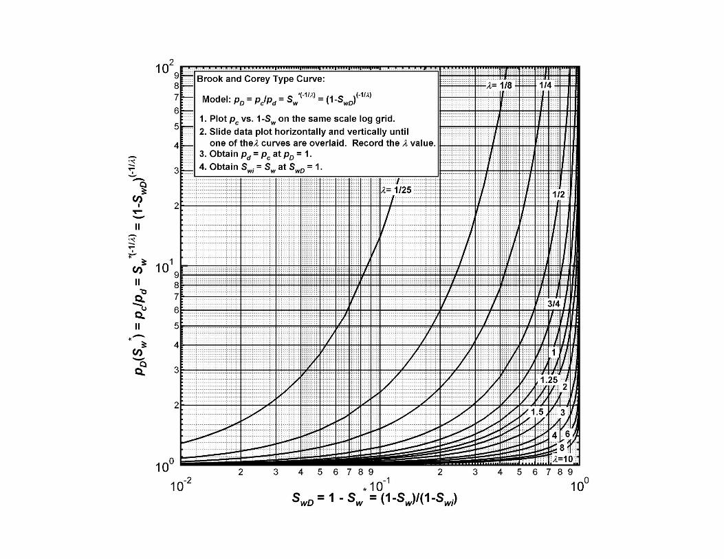
5.3.b For each pc data set you are to determine the pd, Swi, and parameters in the Brooks-Corey pc model using the "type curve" approach given in the notes. The type curve and data grid plot are attached.

Governing Equations:

Brooks-Corey Capillary Pressure Model

where,

pc = Capillary pressure, psiapd = Displacement (or threshold) pressure, psiaSw = Wetting phase saturation, fractionSwi = Irreducible wetting phase saturation, fraction = Brooks-Corey exponent, dimensionless