Embed Size (px)
Citation preview
Pacific-wide sustainability risk assessment of bigeye thresher shark (Alopias superciliosus)
Pacific-wide sustainability risk assessment of bigeye thresher
shark (Alopias superciliosus)
Final Report
Prepared for Western and Central Pacific Fisheries Commission
September 2016
Pacific-wide sustainability risk assessment of bigeye thresher shark (Alopias superciliosus)
Prepared by: Dan Fu1, Marie-Julie Roux1, Shelley Clarke2, Malcolm Francis1, Alistair Dunn1 and Simon Hoyle3
1 National Institute of Water and Atmospheric Research, Wellington, New Zealand
2 ABNJ Tuna Project (Common Oceans), Western and Central Pacific Fisheries Commission, Pohnpei, Federated States of Micronesia
3 National Institute of Water and Atmospheric Research, Nelson, New Zealand
For any information regarding this report please contact: Rosemary Hurst Chief Scientist Fisheries +64-4-386 0867 [email protected] National Institute of Water & Atmospheric Research Ltd Private Bag 14901 Kilbirnie Wellington 6241 Phone +64 4 386 0300
NIWA CLIENT REPORT No: 2016089WN Report date: September 2016 NIWA Project: WCP16301
Quality Assurance Statement
Reviewed by: Dr. Rosemary Hurst
Formatting checked by: Chloe Hauraki
Approved for release by: Dr. Rosemary Hurst
Pacific-wide sustainability risk assessment of bigeye thresher shark (Alopias superciliosus)
Contents
EXECUTIVE SUMMARY ......................................................................................................... 1
LIST OF ACRONYMS ............................................................................................................. 3
1 INTRODUCTION ......................................................................................................... 4
2 DATASETS .................................................................................................................. 8
2.1 CES longline logsheet (commercial effort) data ....................................................... 8
2.2 SPC observer data ..................................................................................................... 9
2.3 US observer data ..................................................................................................... 12
2.4 Japanese observer data .......................................................................................... 14
2.5 Composite dataset .................................................................................................. 15
3 APPROACH AND METHODS ...................................................................................... 18
3.1 Analytical approach ................................................................................................ 18
3.2 Spatial and temporal domains of the assessment .................................................. 19
3.3 Catch groups and fishery groups definition ............................................................ 20
3.4 Species distribution estimation .............................................................................. 23
3.5 Catchability estimation ........................................................................................... 26
3.6 Impact estimation (fishing mortality) ..................................................................... 31
3.7 Population productivity and MIST estimation ........................................................ 32
3.8 Sustainability risk calculations ................................................................................ 34
4 ASSESSMENT RESULTS ............................................................................................. 34
4.1 Species distribution................................................................................................. 34
4.2 Catchability ............................................................................................................. 38
4.3 Fishing impacts ....................................................................................................... 45
4.4 Sustainability risk .................................................................................................... 50
5 DISCUSSION AND RECOMMENDATIONS ................................................................... 56
5.1 Fishery groups ......................................................................................................... 57
5.2 Species distribution................................................................................................. 58
5.3 Catchability ............................................................................................................. 59
5.4 Post-capture survival .............................................................................................. 61
5.5 Maximum impact sustainable threshold (MIST) ..................................................... 62
Pacific-wide sustainability risk assessment of bigeye thresher shark (Alopias superciliosus)
5.6 Sustainability risk .................................................................................................... 63
5.7 Recommendations for future developments and implementations ...................... 64
6 ACKNOWLEDGMENTS .............................................................................................. 65
7 REFERENCES ............................................................................................................ 66
Appendix A – CPUEΩ estimation and derivation ................................................................. 71
Appendix B – BDM description .......................................................................................... 72
Appendix C – q adjustment by fishery groups and spatial scaling ........................................ 74
Appendix D – Observer data characterisation ..................................................................... 75
Appendix E – Spatial standardisations ................................................................................ 77
Appendix F – q calibration Results and sensitivities ............................................................ 85
Appendix G – Catch history ................................................................................................ 90
Appendix H – Year effects standardisations ........................................................................ 91
Appendix I - Impact sensitivity ........................................................................................... 95
Appendix J - Supporting information .................................................................................. 98
Pacific-wide sustainability risk assessment of bigeye thresher shark 1
EXECUTIVE SUMMARY The bigeye thresher shark, Alopias superciliosus, has been identified as one of the least productive pelagic sharks and there is concern about its conservation status. Although it is one of three thresher sharks designated by Western and Central Pacific Fisheries Commission as key shark species, no Pacific Ocean stock assessment has been conducted. Information gaps and changes in reporting and observer coverage over time and space, make traditional approaches to stock assessment impractical. As an alternative and to gain new insights into the sustainability status of bigeye thresher shark, this study applies a spatially explicit and quantitative sustainability risk assessment to available data. The analytical framework evaluates sustainability risk as the ratio of current impacts from fisheries (spatially-explicit and cumulative fishing mortality F) to a maximum impact sustainable threshold (MIST) reference point based on population productivity. This approach differs from traditional stock assessment because it evaluates F in terms of whether the population’s ability to withstand fishing pressure is exceeded, rather than evaluating biomass (B) and whether the population is overfished.
Key components (and analytical procedures) included: 1) estimation of the species distribution or relative abundance in space; 2) calibration of population and fishery groups catchability; and 3) estimation of the maximum intrinsic population growth rate r for the species, using available life history data. The first two components were used in conjunction with commercial effort (logsheet) data to quantify fishing impact. The third was used to define the MIST reference point. A scenario-based approach to sustainability risk evaluation was implemented, with scenarios ranging from more to less precautionary and representing different species distribution, initial population status, maximum density and post-capture survival assumptions. This approach served to cope with currently high levels of uncertainty in population status, movements and biology, and limited information about some aspects of the available datasets. Observer data from the Pacific Community (SPC), United States (US) and Japan were standardized with two models, a zero-inflated negative binomial (ZINB) model and a geo-statistical delta-generalised linear mixed (delta-GLMM) model, which permitted derivation of spatial indices of relative abundance over different but overlapping areas. Population catchability (q) was statistically calibrated using a Bayesian state-space biomass dynamics model (BDM) fitted to time series of relative abundance and annual catch estimates obtained from a representative subset of the observer data. This approach assumed that although the available data were insufficient to estimate absolute catchability, they could be used to calibrate a relative catchability parameter for use in spatially-explicit impact estimation. A range of plausible q values were estimated, with uncertainty, and adjusted spatially by fishing season and catch group (i.e., ‘fishery groups’), as well as for the occurrence of post-capture survival. Fishing mortality was calculated as the sum product of total effort and fishery-group specific catchability in 5x5 degree cells, weighted by the relative density of bigeye thresher shark in each cell, as obtained from the spatial standardization.
The distribution of the maximum population growth rate r had a median value of 0.03, which is higher than previously reported for the species, and was used to define the MIST. Analyses performed assuming 100% capture mortality produced median F values ranging from 0.02 to 0.04 among base case scenarios for the period 2000-2014. Sustainability risk, corresponding to the ratio of total impact to the MIST, ranged from 0.6 to 1.2. The average probability that fishing impact exceeded the MIST was 0.4 across years and scenarios. Analyses performed assuming a range of post-capture survival rates produced median F values ranging from 0.01 to 0.03 and median sustainability risk between 0.4 and 1.0, with an average probability of 0.20 of total fishing impact exceeding the MIST.
2 Pacific-wide sustainability risk assessment of bigeye thresher shark
Earlier studies indicated that the species is vulnerable to exploitation owing to limited productivity, even at relatively low levels of fishing mortality. Sustainability risk results presented here, which incorporate considerable uncertainty both within and among scenarios, are not inconsistent with this view. They suggest that total impacts from pelagic longline fisheries in the Pacific since 2000 are generally low (<5%), but have exceeded the maximum impact sustainable threshold for bigeye thresher in some years.
Risk outcomes were sensitive to q calibration assumptions used in the Biomass Dynamic Model (BDM), namely values of the prior bounds for the unfished biomass at equilibrium (K), initial stock status (biomass in the first year of the model relative to K), and process error inclusion. The implications of such assumptions and sensitivities are discussed in the report, along with potential means of refining impact estimation in future work. Better information on initial stock status, biomass at unfished equilibrium and post-capture survival assumptions, would serve to weight alternative scenarios and improve the accuracy of sustainability risk estimation.
The strengths and value of a spatially-explicit, sustainability risk assessment framework reside in data integration from multiple sources and the ability to map relative fishing impact and sustainability risk spatially and among fishery sectors, with uncertainty.
Pacific-wide sustainability risk assessment of bigeye thresher shark 3
LIST OF ACRONYMS
ABNJ Areas Beyond National Jurisdiction (or Common Oceans)
AFFRC Agriculture, Forestry and Fisheries Research Council, Japan
ALB Albacore Tuna (Thunnus alalunga)
BET Bigeye Tuna (Thunnus obesus)
BTH Bigeye Thresher Shark (Alopias superciliosus)
CES Tuna Fishery Catch and Effort Query System
HBF number of hooks between floats
IATTC Inter-American Tropical Tuna Commission
ICCAT International Convention for the Conservation of Atlantic Tunas
IOTC Indian Ocean Tuna Commission
JP Japan
MIST Maximum impact sustainable threshold
MLS Striped marlin (Kajikia audax)
NOAA National Oceanographic and Atmospheric Administration
ROP Regional Observer Program
SPC The Pacific Community
SST Sea surface temperature
SWO Broadbill Swordfish (Xiphias gladius)
TCSB Tuna Project Technical Coordinator Sharks and Bycatch
TUBS Tuna Fisheries Observer System
US United States
YFT Yellowfin Tuna (Thunnus albacares)
WCPFC Western and Central Pacific Fisheries Commission
WCPO Western and Central Pacific Ocean
4 Pacific-wide sustainability risk assessment of bigeye thresher shark
1 INTRODUCTION The Western and Central Pacific Fisheries Commission (WCPFC) is one of five tuna Regional Fisheries Management Organizations (t-RFMOs) responsible for the sustainable use, conservation and management of highly migratory species taken by tuna fisheries. Unlike some of the other t-RFMOs, the WCPFC has explicit responsibility for assessing and managing not only tuna species, but also dependent and associated species under Articles 5(d) and 10.1(c) of its Convention. Recognition by the WCPFC of sharks as dependent and associated species in need of conservation and management has resulted in a list of thirteen shark species found in the Western and Central Pacific Ocean (WCPO) for which both data provision and assessment are required (WCPFC 2012). The three thresher shark species of the family Alopiidae (Alopias superciliosus, bigeye thresher; A. pelagicus, pelagic thresher; and A. vulpinus, common thresher) have been included in this list since its original formulation in 2008. Thus far, the WCPFC has conducted stock assessments for three of the shark species on the key shark list: oceanic whitetip shark (Carcharhinus longimanus), silky shark (Carcharhinus falciformis) and North Pacific blue shark (Prionace glauca) (Rice & Harley 2012, 2013; Rice et al. 2014). A stock assessment for South Pacific blue shark is currently underway.
Indicator analyses for the thresher sharks were conducted by the WCPFC’s Scientific Services Provider, the Pacific Community (SPC), in 2011 and 2015 (Clarke et al. 2011, Rice et al. 2015). In both cases, most of the analyses were performed at the family level due to presence of a substantial number of non-species specific observer records. The most recent of these analyses hinted at a declining index of abundance for the thresher group as a whole based on decreased catch rates in 2012-2014 and an overall decline since 2003 (Rice et al. 2015). On this basis, the WCPFC Scientific Committee in August 2015 recognized assessment of thresher sharks as a priority.
The WCPFC, along with the four t-RFMOs, is a partner in the Areas Beyond National Jurisdiction (ABNJ) – also referred to as Common Oceans – Tuna Project (www.commonoceans.org). The objective of the ABNJ Tuna Project is to achieve efficient and sustainable management of fisheries resources and biodiversity conservation in marine areas that do not fall under the responsibility of any one country. One set of activities of the GEF-funded ABNJ Tuna Project aims at reducing the impact of tuna fisheries on biodiversity by improving data and assessment methods for sharks and thereby promoting their sustainable management. Within this set of activities WCPFC has committed to leading four new stock status assessment studies for Pacific-wide shark stocks. The bigeye thresher shark was identified as the thresher species with the widest distribution and the greatest number of catch records from the WCPO (Matsunaga and Yokawa 2013, Rice et al. 2015), and it is likely to be the most vulnerable of the three threshers to longline fishing (WCPFC 2006, IOTC 2012, ICCAT 2015), so it was chosen as the best candidate for assessment. A bigeye thresher shark stock status assessment meets the criteria for ABNJ funding as this species has a Pacific-wide distribution, was identified as a priority assessment by at least one of the t-RFMOs, and provides an opportunity to further develop methods for data-poor species.
Biology and distribution
In the Pacific, the bigeye thresher shark primarily occurs in tropical waters, however its habitat ranges as far north as central Japan and Baja California and as far south as the North Island of New Zealand and the southern coast of Peru (Matsunaga & Yokawa 2013). This species is found near the surface at night and makes deep dives to experience temperatures of 6-11oC (up to 500 m depth) during the day,
Pacific-wide sustainability risk assessment of bigeye thresher shark 5
perhaps aided by its rete mirabile, a structure within the orbital sinus believed to help stabilize brain and eye temperatures (Nakano et al. 2003, Weng & Block 2004). Studies from the Atlantic suggest that juveniles concentrate primarily in the tropical North Atlantic, and pregnant females are found at higher latitudes off West Africa and Brazil (Fernandez-Carvalho et al. 2015). Findings from the Pacific suggest a slightly different pattern: neonates and juveniles are clustered near 10oN and S latitude, with pregnant females either also at 10oN or at higher latitudes (20-30oN) to the northeast. Few pregnant females have been found south of the equator in the Pacific (Matsunaga & Yokawa 2013).
There is limited information from which to draw any conclusions regarding stock structure for any of the thresher shark species. One unpublished study indicated no population structure in bigeye threshers across what it considered to be the Indo-Pacific (samples from California, Gulf of California, Ecuador, Hawaii, Taiwan and South Africa). However, the sample size was small (n=64) and it used only one type of DNA (mitochondrial control region) (Trejo 2005). Tagging studies of bigeye thresher sharks off Hawaii have reported movements in both northwesterly and easterly directions with a maximum linear displacement of nearly 3,500 km over 240 days (Weng & Block 2004, Musyl et al. 2011).
The bigeye thresher shark is characterized by high juvenile survival and year-round reproduction (i.e. there is no fixed mating or birthing season), but its low fecundity causes it to have low productivity compared to other pelagic sharks and to be highly vulnerable to fisheries which that catch juveniles of this species. In the Pacific, age at maturity was estimated at 12.3-13.4 years for females and 9-10 years for males. The litter size is 2 pups per cycle with a 1:1 sex ratio and the reproductive cycle duration is unknown (Clarke et al. 2015). In a recent ecological risk assessment conducted for pelagic sharks caught by Atlantic longline tuna fisheries, the bigeye thresher was found to have the lowest intrinsic rate of increase (0.009, confidence interval 0.001-0.018), in other words to be the least productive, of the 16 species considered (ICCAT 2012).
Review of population trends
As introduced above, standardized catch rate indicators for Alopias spp. have been produced from SPC data holdings twice under the WCPFC’s Shark Research Plan (Clarke et al. 2011a, Rice et al. 2015). Japanese longline logbook and research and training vessel data catch rate series for threshers as a group were also produced in the earlier round of analysis (Clarke et al. 2011b)1. In the 2011 analyses, no strong trends in standardized catch rates were found for thresher sharks analysed as a group, although the Japanese research and training vessel data indicated a slight increase in catch rates in the central Pacific from the early 2000s through 2008 (the last available data point; Clarke et al. 2011a,b). The Rice et al. (2015) update study, analyzing data through 2014 but excluding data from the US observer programmes, noted that most catches were observed in the longline fishery in an area from 10oS to 20oN and east of 170oE, and the majority of observed individuals were immature. Catch rates rose from 1995-2001 but decreased slightly from 2003-2011 before falling more sharply in 2012-2014. That study thus concluded that the thresher shark complex appeared to be declining though it was noted that the last data point was based on relatively few data and may have exaggerated the trend in the final year (Rice et al. 2015).
1 Note that while the Japanese research and training vessel data recorded the three thresher species separately, the Japanese logbook data do not, and so for the sake of comparison between the two Japanese datasets, as well between the Japanese datasets and the SPC datasets, threshers were analysed as a group.
6 Pacific-wide sustainability risk assessment of bigeye thresher shark
All three studies also examined trends in median size as a potential measure of fishing pressure. The first SPC analysis considered threshers as a group and found statistically significant decreasing median sizes in the central Pacific (Clarke et al. 2011a). The analysis of Japanese research and training vessel data found declines in median size only for pelagic threshers and no trend for bigeye threshers (Clarke et al. 2011b) which suggests that the trends identified by Clarke et al. (2011a) may have been driven by pelagic thresher shark. The Rice et al. (2015) update study noted that thresher sharks as a group showed relatively stable size trends based on a sample of mostly immature females and immature and mature males in the central Pacific (Rice et al. 2015).
The only consistent catch rate time series specific to bigeye thresher shark prior to the current study was an analysis by the United States National Oceanic and Atmospheric Administration (NOAA) in support of a decision regarding whether to list bigeye thresher sharks on the United States Endangered Species Act. The analysis standardized catch rates based on the extensive Hawaii-based longline observer data for 1995-2014. The catch rate in the final year of the series (2014) was nearly double that of the previous year and was the highest on record. As a result, NOAA conducted a sensitivity test by excluding the 2014 data point but concluded that the influence of the 2014 data point was negligible and that abundance was relatively stable (Young et al. 2016).
At present there are no known stock status assessments for the bigeye thresher shark in any ocean, but two studies of pelagic thresher in Taiwanese waters concluded that the stock was slightly over-exploited (Liu et al. 2006, Tsai et al. 2010). NOAA also recently completed a stock assessment for the common thresher shark (Alopias vulpinus) based primarily on data from California and Mexico. That assessment found that fishing mortality for this primarily coastal stock was relatively low (0.08), well below the overfishing threshold, and the stock was at 94% of its unexploited level and so substantially larger than the minimum stock size threshold. Therefore, the assessment concluded that the common thresher shark was unlikely to be in an overfished condition nor to be experiencing overfishing (Teo et al. 2016).
Finally, there have been a number of studies of thresher sharks in the Atlantic Ocean in recent years, but most analyses have been conducted for Alopias species, i.e. at the family level. In this region, the most consistent, comprehensive data sources are logbook and observer records from the United States’ longline fishery in the northwest Atlantic. Selecting the observer data as the more reliable dataset, Young et al. (2016) re-analysed the time series from 1992-2013 for bigeye thresher shark per se. They found no obvious change in the population trend over time and thus concluded that the northwest Atlantic population had stabilized. One older analysis from the southwest Atlantic, quoted in Amorim et al. (2009), indicated increasing catch rates from 1971-1989 and a gradual decrease from 1990-2001. However, the authors noted that during this period a change in the depth of fishing operations also occurred and this may have affected the time series (Amorim et al. 2009). There are no known available catch rate time series for bigeye thresher sharks from the Indian Ocean.
Current conservation and management designations and measures
The IUCN Red List classifies all three thresher species as “Vulnerable” (IUCN 2015). The Red List assessment for the bigeye thresher shark dates from 2007 and is supplemented by regional assessments of “Vulnerable” in the eastern central Pacific, “Endangered” in the northwest and western central Atlantic, “Near Threatened” in the southwest Atlantic, “Data Deficient” in the Mediterranean Sea; and “Vulnerable” in the Indo-West Pacific (Amorim et al. 2009).
Pacific-wide sustainability risk assessment of bigeye thresher shark 7
Two of the five t-RFMOs have adopted conservation and management measures which pertain to bigeye thresher sharks. In 2009, ICCAT adopted a measure requiring all members to prohibit retention of bigeye thresher sharks with the exception of Mexican small-scale coastal fisheries with catches of less than 110 fish (ICCAT Resolution 09-07). IOTC’s measure requires all members to prohibit retention of all species of thresher shark (IOTC Resolution 13/06). In addition to these species-specific measures, starting with ICCAT in 2004 (Recommendation 04-10), and followed by IATTC (Resolution C-05-03) and IOTC (Resolution 05/05) in 2005, WCPFC in 2006 (CMM 2006-05) and CCSBT in 2008, all of the t-RFMOs have adopted a 5% fins-to-carcass ratio as a means of controlling shark finning for all species including thresher sharks (Clarke et al. 2014a).
All three species of thresher sharks were listed on Appendix II of the Convention on the Conservation of Migratory Species of Wild Animals (CMS) in November 2014. CMS Appendix II listing encourages international cooperation towards conservation of shared species. Subsequently, the three thresher species were added to the Convention on Migratory Species (CMS) Memorandum of Understanding (MOU) for Sharks in February 2016. The function of the MOU is to develop a Conservation Plan to guide cooperation between the signatories to CMS Convention as well as other interested stakeholders.
A proposal to list the bigeye thresher shark, along with the pelagic and common threshers as look-alike species, on Appendix II of the Convention on International Trade in Endangered Species of Wild Flora and Fauna (CITES) was first posted on 2 May 2016 and revised on 1 June 2016. The proponents for the proposal include Sri Lanka, the Bahamas, Bangladesh, Benin, Brazil, Burkina Faso, the Comoros, the Dominican Republic, Egypt, the European Union, Fiji, Gabon, Ghana, Guinea, Guinea-Bissau, Kenya, the Maldives, Mauritania, Palau, Panama, Samoa, Senegal, Seychelles and Ukraine. The proposal will be considered at the 17th Conference of the Parties (COP) in Johannesburg, South Africa from 24 September-05 October 2016. If listed, all exports of thresher sharks, including landings in non-flag State ports will require permits to be issued by the flag State CITES Management Authority. Export permits are contingent upon legal acquisition and non-detriment findings (NDFs), the latter of which represents a certification by an authorized CITES Scientific Authority that the proposed export is not detrimental to the survival of the species (Clarke et al. 2014b).
Sustainability status evaluation
This report presents the preliminary results of a Pacific-wide, spatially-explicit sustainability risk assessment of bigeye thresher shark. Risk assessment tools have been developed in response to data limitation problems in the evaluation of fishing effects on non-target species, including sharks and other elasmobranch species (Stobutski et al. 2002, Griffiths et al. 2006, Braccini et al. 2006, Zhou & Griffiths 2008, Cortés et al. 2010, Gallagher et al. 2012). Recent applications have used semi-quantitative approaches (namely productivity-susceptibility analysis) and demographic methods to estimate population productivity, without quantifying total impacts from fisheries or fishing-induced mortality. Such risk assessments applied to pelagic sharks caught in Atlantic pelagic longline fisheries identified bigeye thresher as one of the most vulnerable species to exploitation (Cortés et al. 2008, 2010, 2012).
Herein, we develop and apply a quantitative framework for estimating spatially-explicit fishing mortality and derive a sustainability status for the species as the ratio of total impact to a maximum impact sustainable threshold (MIST) reference point. Rather than following a traditional stock assessment approach, which relies heavily on population processes that for sharks are often poorly understood, this spatially-explicit approach is based on species productivity, inferred distribution and data on the
8 Pacific-wide sustainability risk assessment of bigeye thresher shark
occurrence, characteristics and intensity of fishing. The quantitative framework allows uncertainty to be quantified and propagated throughout the assessment process. An important outcome is that impact, sustainability risk and uncertainty can be partitioned spatially and among fishery sectors, allowing more focused management.
2 DATASETS Review of the potential sources of catch, effort and size data for bigeye thresher in the Pacific identified the following as key data sets: Non-public domain longline catch and effort data for the entire Pacific maintained in the SPC CES
database and accessible to the ABNJ TCSB via the WCPFC Secretariat (“CES longline logsheet data”);
Non-public domain longline observer data maintained by SPC as part of the ROP and on behalf of Australia, the Cook Islands, the Federated States of Micronesia, Fiji, French Polynesia, the Republic of the Marshall Islands, New Caledonia, New Zealand, Samoa, Solomon Islands, Tonga and Vanuatu and accessible to the ABNJ TCSB through data confidentiality agreements with each country for use in the ABNJ Tuna Project (“SPC observer data”);
Non-public domain United States longline observer data provided directly to the ABNJ TCSB for use in the ABNJ Tuna Project under a data confidentiality agreement (“US observer data”);
Non-public domain Japan longline observer data provided to the ABNJ TCSB and to NIWA under a data confidentiality agreement specific to this BTH assessment (“Japan observer data”).
Each of these datasets is described separately below. Data confidentiality agreements necessary to obtain access to the data required for this study have precluded the provision of the majority of datasets described in this report to NIWA. As a result, the ABNJ (Common Oceans) Tuna Project Technical Coordinator-Sharks and Bycatch (ABNJ TCSB) has taken on the role of data manager and has served as an intermediary between NIWA and the raw datasets.
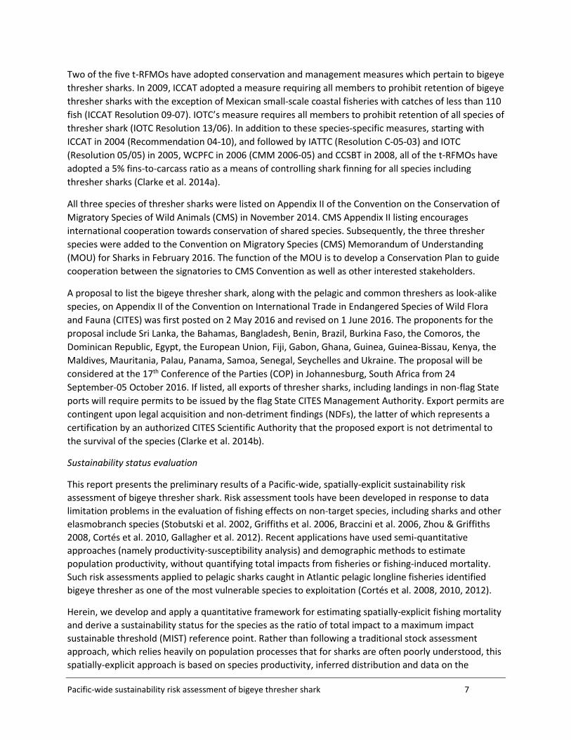
2.1 CES longline logsheet (commercial effort) data The data were downloaded by the ABNJ TCSB from CES on 11 March 2016 and again on 14 April 2016 as there was an update to the data by SPC. The downloaded data consisted of 269,702 records aggregated by year (1950-2014), month (1-12), flag2, and 5 degree latitude by 5 degree longitude (5x5) cell (ranges: -82.5 to 62.5 latitude; 7.5 to 362.5 longitude). The coordinates for each grid represent the southwest corner of each 5x5 cell. Catch data were provided for albacore (ALB), bigeye (BET), Pacific bluefin, skipjack (SKJ), southern bluefin, and yellowfin tunas (YFT); black, blue and striped marlin; Indo-Pacific sailfish; shortbilled spearfish; broadbill swordfish (SWO); blue, “mako”, silky, oceanic whitetip, “thresher” and “other” sharks; and “other”. Annual effort totalled 1.3-1.4 billion hooks in 2011-2013, with lower effort recorded for 2014 likely as a result of incomplete reporting at the time of writing (Figure 1). Overall trends in effort and target species catch in the WCPO longline fishery through 2014 were reviewed by Williams & Terawasi (2015). 2 Flags (countries and fishing entities) include AU, BZ, CK, CN, ES, FJ, FM, GU, ID, JP, KI, KR, MH, NC, NU, NZ, PF, PG, PH, PT, PW, SB, SN, TO, TV, TW, US, VN, VU and WS (see http://www.nationsonline.org/oneworld/country_code_list.htm for code and country name matching)
Pacific-wide sustainability risk assessment of bigeye thresher shark 9
Catch was downloaded in number of sharks as that is the unit used in the observer datasets and is likely to be more accurate than weight-based measures. The total number of “thresher” sharks in the dataset was 129,933 with an annual high of 28,991 in 2014 (data for 2015 were likely incomplete at the time of writing). The first “thresher” shark to be recorded on a logsheet was by Papua New Guinea in 1997; other flags’ first reporting was in 1998 (Samoa), 2000 (US), 2002 (Fiji), 2006 (Spain), 2007 (Australia and New Zealand), 2008 (Japan and Taiwan), 2010 (Korea and New Caledonia), 2011 (Cook Islands), 2013 (FSM and Vanuatu), 2014 (Kiribati) and 2015 (China). These dates probably reflect the year in which the logsheets first provided a space for recording thresher sharks rather than the actual first encounter of a thresher shark by each flag’s fishing vessels.
The CES longline logsheet data were aggregated by year, month, 5x5 cell and flag to obtain the total effort in hooks fished per strata.
Figure 1: Total longline effort for the Pacific Ocean, 1995-2014 as downloaded from the SPC Catch Effort Query System (CES as of April 2016).
2.2 SPC observer data These data were downloaded by the ABNJ TCSB on 3 March 2016 through a special TUBS interface for SPC and WCPFC Secretariat staff. Some issues with large files sizes were encountered which prevented remote downloading of all necessary files at that time; the remaining large data files were received on 8 March 2016. Downloaded data consisted of two files for each fleet and year: one file that contained set-level information with one row per set and one file that contained catch records for individual sharks with one row per shark or ray caught. Length data were provided in some datasets (i.e. SPC and Japan data), but were not formatted for use3. Length data can be used to distinguish life stages of the species, potentially allowing for fishing impacts to be evaluated for different life stage groups, but this requires further development of the
3 Length data presumably exist in the US observer programme data but were not included in the extract provided by the US for this study.
10 Pacific-wide sustainability risk assessment of bigeye thresher shark
methodology in this assessment which has not been undertaken. Fate and condition data were provided and used to distinguish between BTH which were and were not alive upon release. This was accomplished by first removing all BTH which were recorded as unknown either at landing or upon release. Then those with fate codes beginning with R (retained) or DFR (discarded, fins retained), or condition codes A3 (alive but dying) or D (dead) were considered dead and all others were considered to be alive at release. These data could be used to examine the trend in the post-capture survival. Data on BTH sex exist in the SPC observer dataset (Clarke et al. 2011, Rice et al. 2015) but were not included in the subset of data downloadable through the TUBS interface. To link each catch record to its set characteristics, a unique identifier was created by combining set identifiers and trip identifiers in the set database. At this step, 522 set records shared identifiers with another set. As it was impossible to know which, if any, of these set records were correct, all 522 were removed. From the remaining number of sets (n=41,048), containing 3,388 BTH, the following number of sets (and BTH records) were removed sequentially: Removed due to missing lat/long information (1,947 sets and 180 BTH);
Removed due to not being within the year range 1995-2014 (4,791 sets and 51 BTH);
Removed due to missing hooks fished values (715 sets and no BTH);
Removed due to missing hooks between floats (68 sets and no BTH);
Removed due to too many or too few hooks (965 sets and 34 BTH);
Removed due to too many or too few hooks between baskets (220 sets and 7 BTH); and
Removed due to being outside the spatial boundaries of the assessment (4,226 sets and 4 BTH) (see Section 3.1 for the spatial range criteria applied).
Removals related to missing values (hooks between floats, latitude, longitude and number of hooks fished) were necessary because these values are likely to be very important in the standardizations and missing values may interfere with coefficient estimation. Extreme values of hooks fished (i.e. <500 or >4000) were considered to represent abnormal fishing operations and were also thus removed. Similarly, sets recording fewer than four, or more than 45 hooks between baskets were considered dubious and were removed. Finally, sets before 1995 (the year when the SPC regional observer program began in earnest) were removed due to expected poorer data quality in the initial years, and sets after 2014 were removed to avoid biases associated with incomplete reporting.
Pacific-wide sustainability risk assessment of bigeye thresher shark 11
A number of other filters applied or discussed in Rice et al. (2015) were considered but not applied as follows: sets from fisheries known to be targeting sharks (e.g. Papua New Guinea) and those sets for which
the set header field target_shk_yn=yes (Table 3), were not removed a priori as it was considered that any shark targeting effect could be addressed through the catch rate standardization;
removing sets from small national observer programs with < 100 sets each was not considered necessary as this analysis will not be using the observer program identifier in lieu of actual (lat/long) location;
removing records considered to be outside the sea surface temperature (SST) range of species was not done due to doubts about the certainty of bigeye thresher species’ SST range and a preference to address habitat issues through a lat/long exclusion criterion; and
removing records where the catch rate of BTH was greater than the 97.5th percentile of nominal mean CPUE for the dataset as a whole was not done because BTH may exhibit schooling behaviour and thus we might expect to see rare large catches.
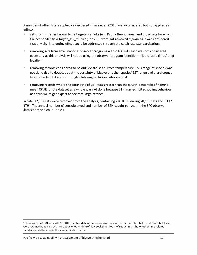
In total 12,932 sets were removed from the analysis, containing 276 BTH, leaving 28,116 sets and 3,112 BTH4. The annual number of sets observed and number of BTH caught per year in the SPC observer dataset are shown in Table 1.
4 There were n=2,001 sets with 183 BTH that had date or time errors (missing values, or Haul Start before Set Start) but these were retained pending a decision about whether time of day, soak time, hours of set during night, or other time-related variables would be used in the standardization model.
12 Pacific-wide sustainability risk assessment of bigeye thresher shark
Table 1: Summary of BTH catch and effort information by year available in the SPC observer dataset.
Year Sets BTH Catch
Records 1995 469 3 1996 485 4 1997 621 9 1998 581 38 1999 456 39 2000 507 61 2001 634 62 2002 1 576 136 2003 1 536 87 2004 1 428 86 2005 1 834 247 2006 2 497 876 2007 1 960 698 2008 1 540 111 2009 1 581 150 2010 1 284 23 2011 1 346 63 2012 1 566 187 2013 3 328 131 2014 2 887 101
The SPC observer dataset is distributed with low coverage over a wide area from 1993-2015. Detailed analysis of thresher shark data in the SPC observer set was conducted by Clarke et al. (2011) and Rice et al. (2015) but it should be noted that most of those analyses were conducted for Alopias spp (see section 1). The spatial distribution of the SPC observer dataset is shown in Figure 2.
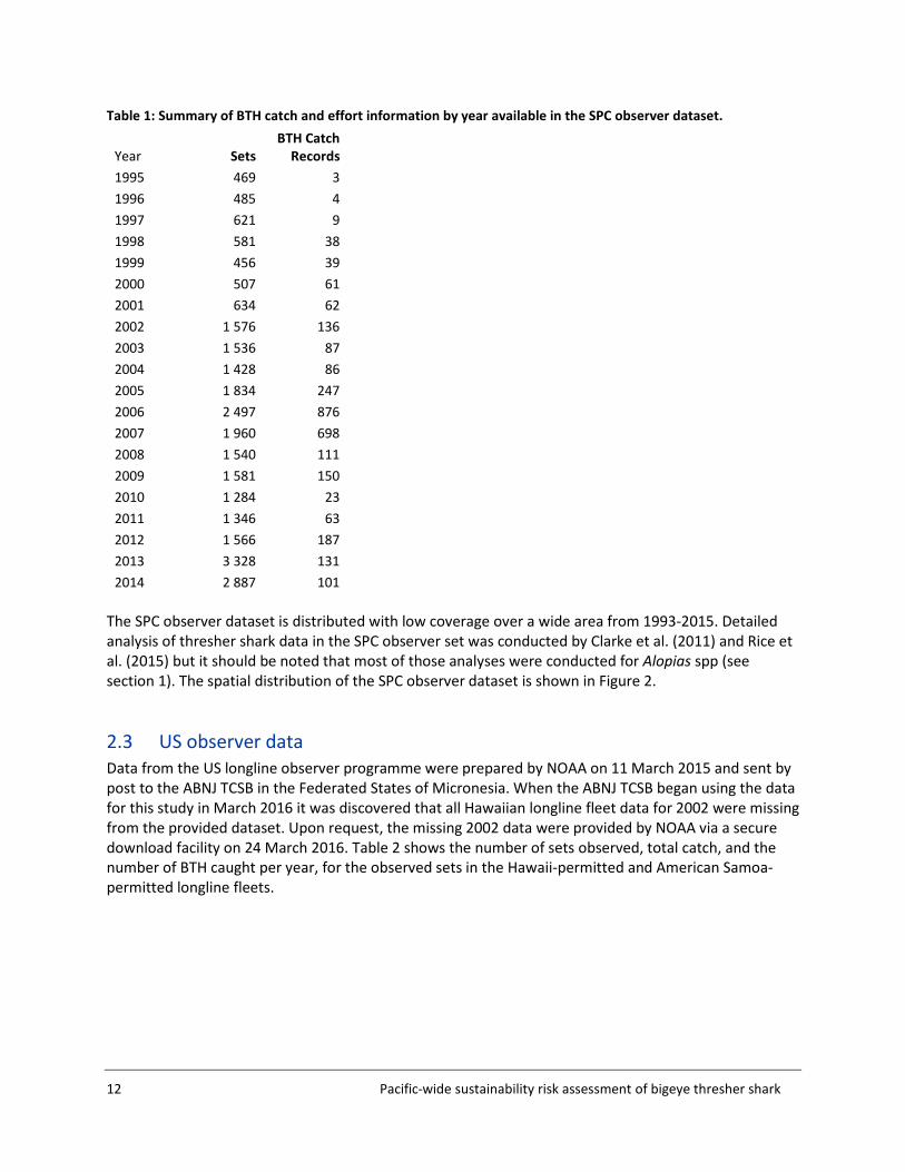
2.3 US observer data Data from the US longline observer programme were prepared by NOAA on 11 March 2015 and sent by post to the ABNJ TCSB in the Federated States of Micronesia. When the ABNJ TCSB began using the data for this study in March 2016 it was discovered that all Hawaiian longline fleet data for 2002 were missing from the provided dataset. Upon request, the missing 2002 data were provided by NOAA via a secure download facility on 24 March 2016. Table 2 shows the number of sets observed, total catch, and the number of BTH caught per year, for the observed sets in the Hawaii-permitted and American Samoa-permitted longline fleets.
Pacific-wide sustainability risk assessment of bigeye thresher shark 13
Table 2: Number of sets observed, total number of fish (etc.) caught, and BTH caught by year in the observed sets of the two fleets covered by the US observer programme and used in this study.
Year Sets Total Catch Records
BTH Catch Records
Sets Total Catch Records
BTH Catch Records
Hawaii-permitted Longline Fishery American Samoa-permitted Longline Fishery
1995 519 26,422 75 0 0 0 1996 587 28,560 208 0 0 0 1997 443 30,507 140 0 0 0 1998 556 31,511 229 0 0 0 1999 421 24,794 83 0 0 0 2000 1,370 69,393 399 0 0 0 2001 2,699 132,214 692 0 0 0 2002 3,296 152,505 1,271 0 0 0 2003 3,078 160,255 765 0 0 0 2004 3,855 186,788 1,789 0 0 0 2005 5,829 274,322 1,158 0 0 0 2006 4,120 180,912 1,521 235 27,100 20 2007 4,762 223,752 1,293 327 40,497 19 2008 4,968 226,722 1,075 266 29,254 19 2009 4,683 199,899 1,660 237 26,167 24 2010 4,958 246,262 1,381 890 100,052 61 2011 4,572 236,003 1,319 1,017 90,357 67 2012 4,639 224,117 1,708 592 57,427 28 2013 4,389 262,919 1,645 584 44,863 49 2014 4,857 279,463 3,828 515 40,115 43 Total 64,601 3,197,320 22,239 4,663 455,832 330
Length and sex data may exist in the US observer dataset but were not included in the subset provided for this study. Regarding fate and condition classification, the US observer programme only records shark condition at retrieval as alive or dead, and at release as alive, dead or kept. This simplified distinguishing between BTH which did and did not survive until release. As for the SPC observer data, a number of filters were considered to clean and format the US observer data (see section 2.3). Of these, six filters were applied with the following results: Removed due to missing lat/long information (9 sets and 1 BTH);
Removed due to missing hooks fished values (6 sets and no BTH);
Removed due to missing hooks between floats (22 sets and 8 BTH);
Removed due to too many or too few hooks (293 sets and 17 BTH);
Removed due to too many or too few hooks between baskets (186 sets and 9 BTH); and
Removed due to being outside the spatial boundaries of the assessment (551 sets and 11 BTH) (see section 3.1 for the spatial range criteria applied).
In total 1,067 sets were removed from the analysis, containing 46 BTH, leaving 69,264 sets and 22,523 BTH.
14 Pacific-wide sustainability risk assessment of bigeye thresher shark
The US observer dataset is a rich source of BTH data with considerably more records for this species than the SPC dataset (22,523 BTH in 69,264 sets versus 3,112 BTH in 28,116 sets). The spatial distribution of the US observer dataset is shown in Figure 2.
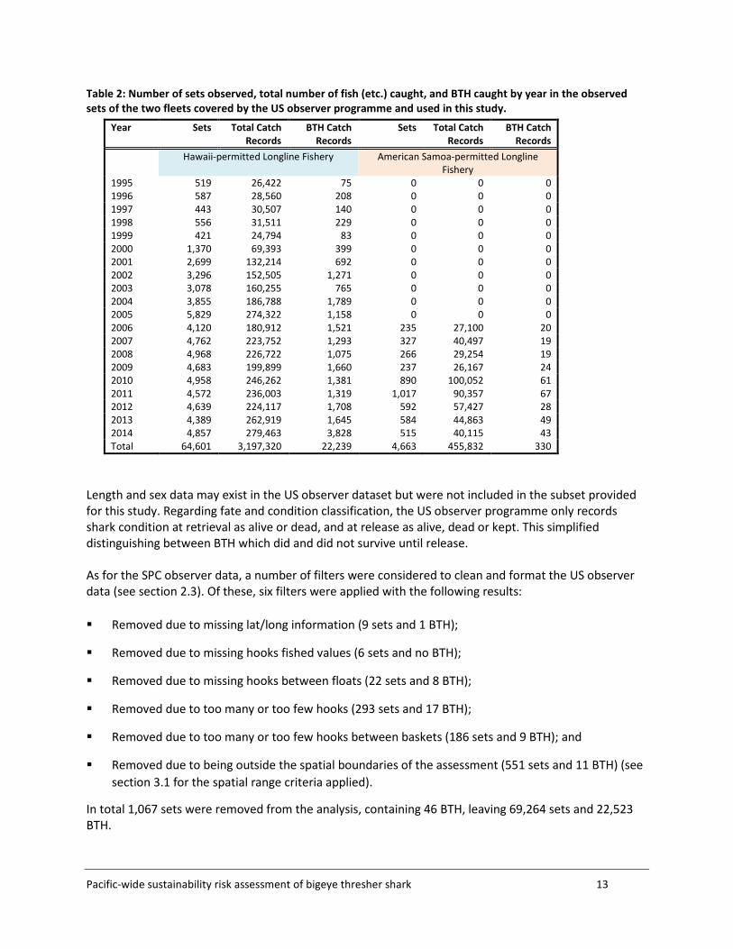
2.4 Japanese observer data Japan’s longline observer program has been operating since 2007 but has only been fully implemented since 2011. A data confidentiality agreement was negotiated between the Japan Fisheries Agency, NIWA and the ABNJ (Common Oceans) Tuna Project on 24 March 2016. Data were provided using a secure internet file sharing system on the same day and re-provided on 25 March 2016 to correct minor formatting errors. The number of sets observed, total number of thresher sharks caught and the number of BTH caught per year for the observed Japanese longline sets as received are shown in Table 3.
Table 3: Number of sets observed, total number of threshers caught, and BTH caught by year in the observed sets of the Japanese longline fleet as provided by Japan. Note that Japan did not provide catch records for species other than thresher sharks (bigeye, pelagic, common and unknown).
Year Sets Total Catch of Threshers Catch of BTH 2007 13 4 4 2008 143 27 20 2009 89 4 2 2010 162 183 28 2011 638 275 152 2012 908 357 57 2013 1,756 972 376 2014 1,877 788 513 2015 1,371 355 171 Total 6,957 2965 1323
Length data were provided for 949 BTH and sex data for 939 BTH. These data have not yet been formatted for use. Fate and condition data were not provided. Filters were considered and applied as for the other observer data (see section 2.3). Of these, six filters were applied with the following results: Removed due to missing lat/long information (317 sets and 28 BTH);
Removed due to missing hooks fished values (1 set and 3 BTH);
Removed due to missing hooks between floats (33 sets and 20 BTH);
Removed due to being outside the spatial boundaries of the assessment (218 sets and 6 BTH) (see section 3.1 for the spatial range criteria applied).
In total 569 sets were removed from the analysis, containing 57 BTH, leaving 6,405 sets and 1,266 BTH. The Japan observer dataset contains 1,266 BTH from 6,405 sets. The number of BTH per set in the Japan observer dataset (0.20) is intermediate between that of the SPC observer dataset (0.11) and the US observer dataset (0.33). The spatial distribution of the Japanese observer dataset is shown in Figure 2.
Pacific-wide sustainability risk assessment of bigeye thresher shark 15
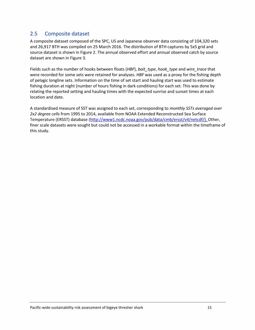
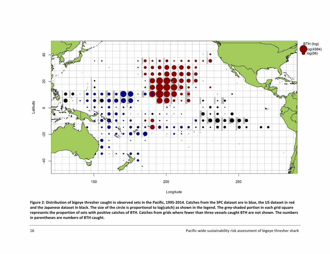
2.5 Composite dataset A composite dataset composed of the SPC, US and Japanese observer data consisting of 104,320 sets and 26,917 BTH was compiled on 25 March 2016. The distribution of BTH captures by 5x5 grid and source dataset is shown in Figure 2. The annual observed effort and annual observed catch by source dataset are shown in Figure 3. Fields such as the number of hooks between floats (HBF), bait_type, hook_type and wire_trace that were recorded for some sets were retained for analyses. HBF was used as a proxy for the fishing depth of pelagic longline sets. Information on the time of set start and hauling start was used to estimate fishing duration at night (number of hours fishing in dark conditions) for each set. This was done by relating the reported setting and hauling times with the expected sunrise and sunset times at each location and date. A standardised measure of SST was assigned to each set, corresponding to monthly SSTs averaged over 2x2 degree cells from 1995 to 2014, available from NOAA Extended Reconstructed Sea Surface Temperature (ERSST) database (http://www1.ncdc.noaa.gov/pub/data/cmb/ersst/v4/netcdf/). Other, finer scale datasets were sought but could not be accessed in a workable format within the timeframe of this study.
16 Pacific-wide sustainability risk assessment of bigeye thresher shark
Figure 2: Distribution of bigeye thresher caught in observed sets in the Pacific, 1995-2014. Catches from the SPC dataset are in blue, the US dataset in red and the Japanese dataset in black. The size of the circle is proportional to log(catch) as shown in the legend. The grey-shaded portion in each grid square represents the proportion of sets with positive catches of BTH. Catches from grids where fewer than three vessels caught BTH are not shown. The numbers in parentheses are numbers of BTH caught.
Pacific-wide sustainability risk assessment of bigeye thresher shark 17
Figure 3: Total observed effort (in million hooks) by data source (top panel) and total number of BTH observed by data source (bottom panel), 1995-2014.
18 Pacific-wide sustainability risk assessment of bigeye thresher shark
3 APPROACH AND METHODS
3.1 Analytical approach The analytical framework is risk-based and spatially-explicit. Sustainability status S is assessed relative to current impacts from fisheries (or relative fishing mortality F) and a maximum impact sustainable threshold (MIST) limit reference point (LRP):
LRPF
MISTImpact
≈=S
Uncertainty in all parameters is quantified and propagated through the assessment framework. In this context, sustainability risk R is the probability p, given the uncertainty, that the total impact exceeds the MIST:
MIST]Impact p[ >=R
The assessment is conducted over a spatial grid of 5 by 5 degree latitude and longitude cells (section 3.2). Fishing impact is estimated as the average of fishing mortality iF weighted by species relative
abundance in in each cell:
∑∑
=
ii
iii
n
nFImpact
Cell-specific iF is calculated as the product of fishing effort E and catchability q distinguished among (and summed across) fishery groups j :
∑=j
jjii qEF ,
where jq expresses the fraction of the total population in each cell that is available for capture by each unit of effort, adjusted for capture efficiency in fishery group j .
Effort differentiation into fishery groups serves to handle the effects of different fishing operations and operational practices on total impact. Impacts are assumed to be cumulative across fishery groups and over the spatial domain of the assessment. As a result, sustainability risk, fishing impact and uncertainty can be disaggregated in space and among fishery sectors.
MIST is the sustainable reference threshold for the species. The MIST is defined based on population productivity inferred from life history data. Life history parameters are used to estimate a maximum intrinsic population growth rate r, with uncertainty. In turn, r is used to derive sustainable impact thresholds similar to the fishing mortality-based sustainability reference points (Fcrash,Fmsm, Flim) described by Zhou et al. (2011).
The assessment is implemented in a flexible framework allowing incremental improvements and fine-tuning as data are augmented and/or better information becomes available.
Pacific-wide sustainability risk assessment of bigeye thresher shark 19
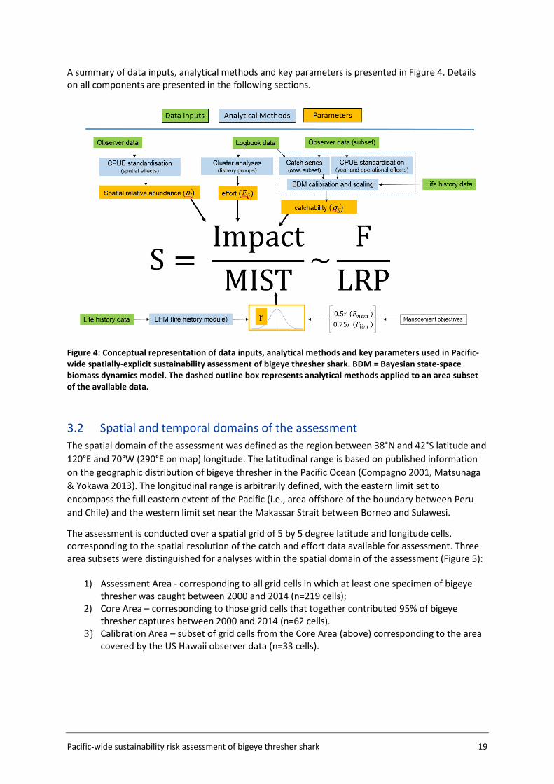
A summary of data inputs, analytical methods and key parameters is presented in Figure 4. Details on all components are presented in the following sections.
Figure 4: Conceptual representation of data inputs, analytical methods and key parameters used in Pacific-wide spatially-explicit sustainability assessment of bigeye thresher shark. BDM = Bayesian state-space biomass dynamics model. The dashed outline box represents analytical methods applied to an area subset of the available data.
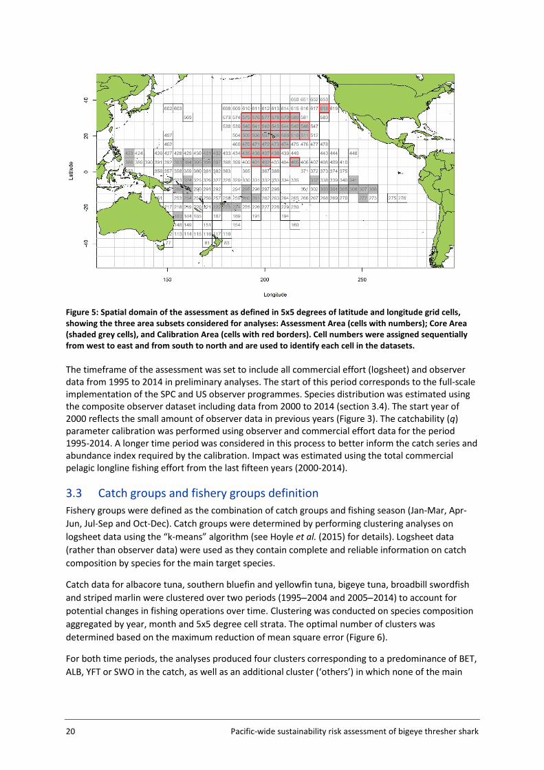
3.2 Spatial and temporal domains of the assessment The spatial domain of the assessment was defined as the region between 38°N and 42°S latitude and 120°E and 70°W (290°E on map) longitude. The latitudinal range is based on published information on the geographic distribution of bigeye thresher in the Pacific Ocean (Compagno 2001, Matsunaga & Yokawa 2013). The longitudinal range is arbitrarily defined, with the eastern limit set to encompass the full eastern extent of the Pacific (i.e., area offshore of the boundary between Peru and Chile) and the western limit set near the Makassar Strait between Borneo and Sulawesi.
The assessment is conducted over a spatial grid of 5 by 5 degree latitude and longitude cells, corresponding to the spatial resolution of the catch and effort data available for assessment. Three area subsets were distinguished for analyses within the spatial domain of the assessment (Figure 5):
1) Assessment Area - corresponding to all grid cells in which at least one specimen of bigeye thresher was caught between 2000 and 2014 (n=219 cells);
2) Core Area – corresponding to those grid cells that together contributed 95% of bigeye thresher captures between 2000 and 2014 (n=62 cells).
3) Calibration Area – subset of grid cells from the Core Area (above) corresponding to the area covered by the US Hawaii observer data (n=33 cells).
20 Pacific-wide sustainability risk assessment of bigeye thresher shark
Figure 5: Spatial domain of the assessment as defined in 5x5 degrees of latitude and longitude grid cells, showing the three area subsets considered for analyses: Assessment Area (cells with numbers); Core Area (shaded grey cells), and Calibration Area (cells with red borders). Cell numbers were assigned sequentially from west to east and from south to north and are used to identify each cell in the datasets. The timeframe of the assessment was set to include all commercial effort (logsheet) and observer data from 1995 to 2014 in preliminary analyses. The start of this period corresponds to the full-scale implementation of the SPC and US observer programmes. Species distribution was estimated using the composite observer dataset including data from 2000 to 2014 (section 3.4). The start year of 2000 reflects the small amount of observer data in previous years (Figure 3). The catchability (q) parameter calibration was performed using observer and commercial effort data for the period 1995-2014. A longer time period was considered in this process to better inform the catch series and abundance index required by the calibration. Impact was estimated using the total commercial pelagic longline fishing effort from the last fifteen years (2000-2014).
3.3 Catch groups and fishery groups definition Fishery groups were defined as the combination of catch groups and fishing season (Jan-Mar, Apr-Jun, Jul-Sep and Oct-Dec). Catch groups were determined by performing clustering analyses on logsheet data using the “k-means” algorithm (see Hoyle et al. (2015) for details). Logsheet data (rather than observer data) were used as they contain complete and reliable information on catch composition by species for the main target species.
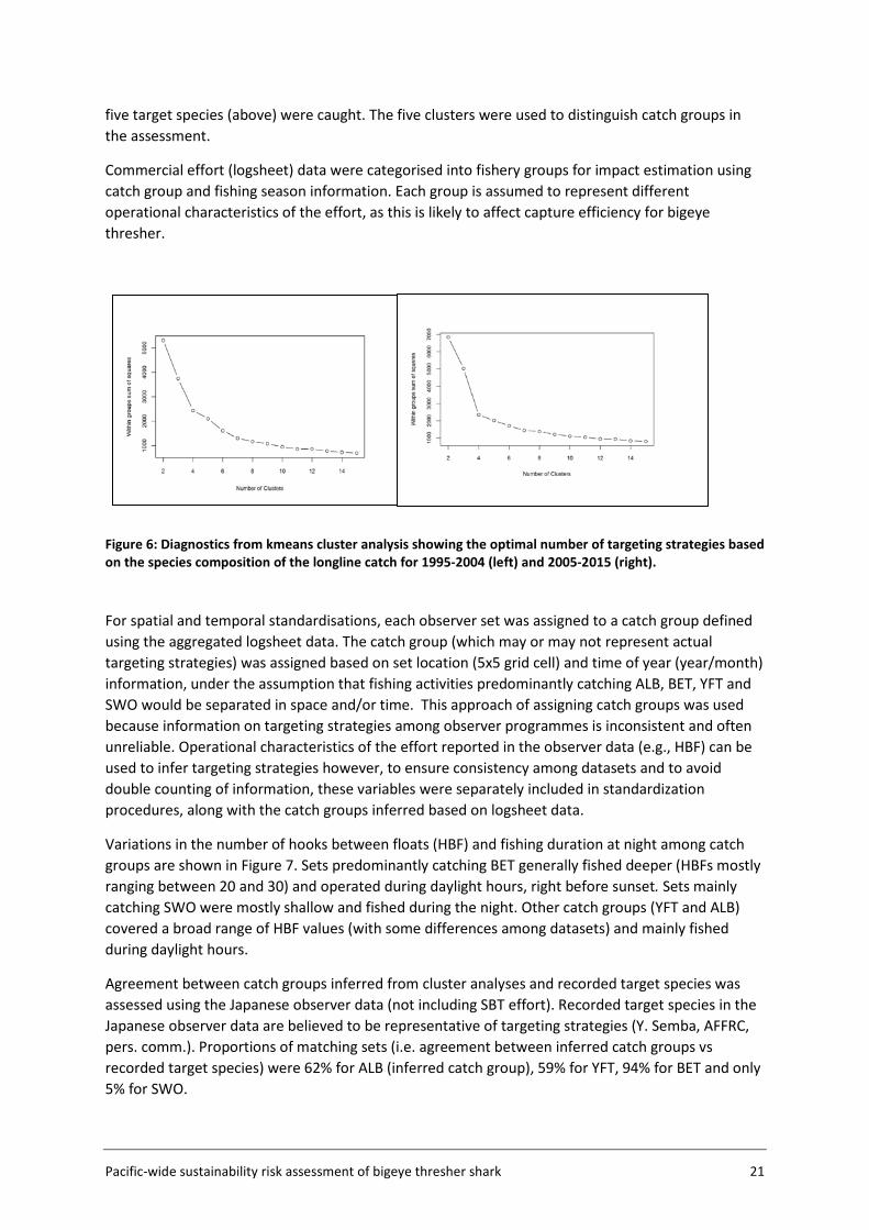
Catch data for albacore tuna, southern bluefin and yellowfin tuna, bigeye tuna, broadbill swordfish and striped marlin were clustered over two periods (1995−2004 and 2005−2014) to account for potential changes in fishing operations over time. Clustering was conducted on species composition aggregated by year, month and 5x5 degree cell strata. The optimal number of clusters was determined based on the maximum reduction of mean square error (Figure 6).
For both time periods, the analyses produced four clusters corresponding to a predominance of BET, ALB, YFT or SWO in the catch, as well as an additional cluster (‘others’) in which none of the main
Pacific-wide sustainability risk assessment of bigeye thresher shark 21
five target species (above) were caught. The five clusters were used to distinguish catch groups in the assessment.
Commercial effort (logsheet) data were categorised into fishery groups for impact estimation using catch group and fishing season information. Each group is assumed to represent different operational characteristics of the effort, as this is likely to affect capture efficiency for bigeye thresher.
Figure 6: Diagnostics from kmeans cluster analysis showing the optimal number of targeting strategies based on the species composition of the longline catch for 1995-2004 (left) and 2005-2015 (right).
For spatial and temporal standardisations, each observer set was assigned to a catch group defined using the aggregated logsheet data. The catch group (which may or may not represent actual targeting strategies) was assigned based on set location (5x5 grid cell) and time of year (year/month) information, under the assumption that fishing activities predominantly catching ALB, BET, YFT and SWO would be separated in space and/or time. This approach of assigning catch groups was used because information on targeting strategies among observer programmes is inconsistent and often unreliable. Operational characteristics of the effort reported in the observer data (e.g., HBF) can be used to infer targeting strategies however, to ensure consistency among datasets and to avoid double counting of information, these variables were separately included in standardization procedures, along with the catch groups inferred based on logsheet data.
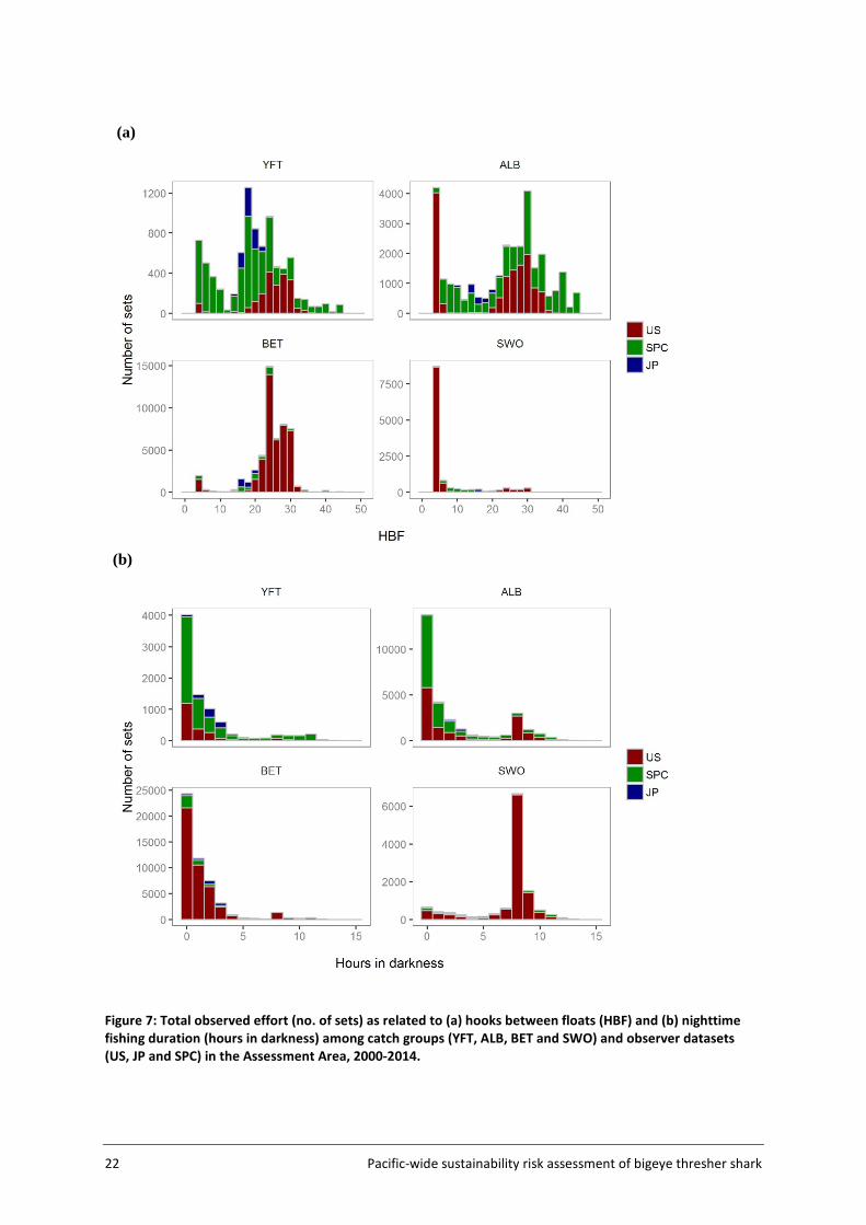
Variations in the number of hooks between floats (HBF) and fishing duration at night among catch groups are shown in Figure 7. Sets predominantly catching BET generally fished deeper (HBFs mostly ranging between 20 and 30) and operated during daylight hours, right before sunset. Sets mainly catching SWO were mostly shallow and fished during the night. Other catch groups (YFT and ALB) covered a broad range of HBF values (with some differences among datasets) and mainly fished during daylight hours.
Agreement between catch groups inferred from cluster analyses and recorded target species was assessed using the Japanese observer data (not including SBT effort). Recorded target species in the Japanese observer data are believed to be representative of targeting strategies (Y. Semba, AFFRC, pers. comm.). Proportions of matching sets (i.e. agreement between inferred catch groups vs recorded target species) were 62% for ALB (inferred catch group), 59% for YFT, 94% for BET and only 5% for SWO.
22 Pacific-wide sustainability risk assessment of bigeye thresher shark
Figure 7: Total observed effort (no. of sets) as related to (a) hooks between floats (HBF) and (b) nighttime fishing duration (hours in darkness) among catch groups (YFT, ALB, BET and SWO) and observer datasets (US, JP and SPC) in the Assessment Area, 2000-2014.
(a)
(b)
Pacific-wide sustainability risk assessment of bigeye thresher shark 23
3.4 Species distribution estimation
3.4.1 Approach and input data Standardisation analyses performed on observer catch and effort data were used to infer the spatial distribution of bigeye thresher. The composite observer dataset for the period 2000-2014 was used. Data from 1995-1999 were excluded owing to comparatively limited spatial and numerical coverage. Two standardisation models were applied for comparison: a zero-inflated negative binomial model (ZINB) (Zuur et al. 2009) and a geo-statistical delta-generalised linear mixed model (delta-GLMM) (Thorson et al. 2015). Both were used to standardise catch rates of bigeye thresher in 5x5 degree cells. The standardised catch rates or relative densities are assumed to be representative of spatial abundance distribution for the species. Data from all observed longline sets were included in the spatial standardisations (i.e., no representative ‘fishery subset’ was defined for the species). Outputs from both models as well as strengths and limitations are compared and discussed in the context of spatially-explicit sustainability risk assessment for pelagic shark species.
3.4.2 ZINB standardisation ZINB models serve to handle overdispersed count data with excessive number of zeros (Zuur et al. 2009). The relationship between the response variable (in this case, the number of bigeye thresher caught per set) and a set of explanatory variables is modelled as a mixture of an encounter probability (binomial process) and a negative binomial count process (that allows for overdispersion and zero occurrences). The estimation of spatial effects in each grid cell requires a large number of coefficients to be estimated. To reduce the number of parameters and improve estimation, the fitting of the ZINB model was restricted to observer catch and effort data from the Core Area (Figure 5, section 3.2). This was required to ensure successful model convergence. Likewise, convergence problems caused by the estimation of a large number of coefficients precluded the inclusion of vessel effects in the ZINB model. The implication of this is that the abundance outside the Core Area is assumed to be very low so that its contribution to the overall fishing impact on the whole population is negligible. Explanatory variables considered in spatial standardisations are listed in Table 4. A number of variables including bait_type, hook_type, wire_trace, sst and night_fishing were included in preliminary analyses but excluded from the final models due to missing or ambiguous values (wire_trace and hook_type); too many values (too many coefficients to be estimated and no clear basis for grouping) (bait_type); confounding effects with other covariates (night_fishing) and dubious relationships to the response variable (sst). Other variables were offered sequentially, producing a series of nested models. The same sets of variables were offered simultaneously to both the zero and count components of ZINB models. Likelihood ratio tests (performed using function lrtest in R package lmtest (R core development team 2016)) were used to assess the effect of each additional variable on model fit and explanatory power. Alternative models were also compared using AIC (Akaike Information Criterion).
24 Pacific-wide sustainability risk assessment of bigeye thresher shark
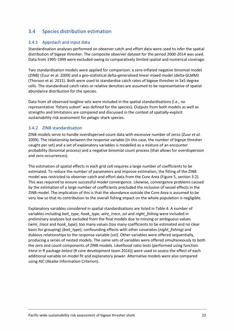
Table 4: Summary of explanatory variables offered to ZINB models for spatial standardisation of catch rates of bigeye thresher in observed pelagic longline fisheries in the Pacific Ocean. Continuous variables were modelled as natural splines with 3 degrees of freedom.
Variable Type Description
year Categorical Calendar year (2000-2014) cell Categorical 5x5 degree grid cells in the Core Area month Continuous Calendar month (1-12)
catch group Categorical Species catch composition log(effort) Offset No. of hooks per set HBF Continuous Hooks between floats
bait_type Categorical Types of bait used hook_type Categorical Types of hooks used wire_trace Categorical Presence/Absence (retention effect)
night_fishing Continuous Fishing duration at night (hours) SST Continuous Sea surface temperature
Spatial indices of relative abundance were derived as the predicted catch rate (no. of bigeye thresher caught per 1000 hooks) for each grid cell in the Core Area, with other covariates fixed to a reference value corresponding to the coefficient calculated for the intercept term (categorical variables) or the median observed value multiplied by the coefficient (continuous variables).
Model fit was assessed using a number of diagnostics plots, including observed versus fitted catch rates, plots of Pearson residuals versus fitted values and Pearson residuals by year and grid cell.
3.4.3 Delta-GLMM standardisation The delta-GLMM model developed by Thorson et al (2015) allows for extrapolation to nearby cells (i.e., density estimation in cells with no observations) by assuming spatially correlated spatial variation. Similar to the ZINB, the delta-GLMM includes a binomial process that models the probability of encounter (i.e., proportion of sets that catch bigeye thresher) and a count process (positive catch rates) that follows a gamma distribution. Additional complexity relates to the integration and differentiation of fixed and random effects.
Random spatial variation and spatiotemporal variation are approximated using Gaussian Markov random fields over a number of ‘knots’. The location of each knot is determined by applying the k-means clustering algorithm to the positional information in the available data (i.e., latitude and longitude data from all sets converted to eastings and northings). This results in a distribution of ‘knots’ with density proportional to sampling intensity (or in this case, fishing intensity as related to observer coverage). The knots define the model’s ‘predictive framework’ and allow for piecewise-constant random fields approximation. This approach has a number of computational advantages and assumes that density at any location is equal to the density value estimated at the nearest knot. The number of knots can be specified within the model framework, allowing control over the accuracy of random effects estimation. This can also be used to achieve a balance of accuracy and computational speed (Thorson et al. 2015). Both the encounter probability and catch process are modelled using a link function and a combination of linear predictors including the random fields. Fixed effects are estimated using maximum marginal likelihood (approximated using the Laplace approximation), while integrating across all random effects. The model is implemented in template model builder (Kristensen et al. 2014).
Pacific-wide sustainability risk assessment of bigeye thresher shark 25
For application to bigeye thresher, year was included as a fixed effect and vessel was included as a random effect in all models. Other variables considered and included as potential linear predictors were fishery groups, HBF and month (see Table 4, section 3.4.2 for details). The number of knots was fixed at 1000 in all runs. The estimation of spatial abundance indices (number of bigeye thresher caught per 1000 hooks) involved a two-step process: 1) fine-scale extrapolation; and 2) density estimation at the spatial scale of the assessment (5x5 degree cells).
The Assessment Area (Figure 5, section 3.2) was subdivided into a fine-scale (10x10 km cells) extrapolation grid. Density extrapolation was restricted to cells with observations (i.e., in which there was a recorded longline set start position) and to cells with no observations but a recorded longline set start position within a maximum distance of 50 km. The resulting predictive framework was composed of 296 045 square grids of 100 km2 each and an extrapolation layer of 1000 knots. Relative abundance at the scale of 5x5 degree cells was calculated as the average density estimated in 10x10km cells in the predictive framework. Three separate delta-GLMM models were fitted and compared: 1) a spatial model (assuming constant spatial variation over time); 2) a spatiotemporal model (allowing spatial variation to differ among years); and 3) a core vessels model (like the spatial model in 1) but including only vessels that caught at least one specimen of bigeye thresher).
Spatial correlation was assessed using geometric anisotropy plots. Estimated vessel effects on encounter probability and positive catch rates were plotted (with 95% confidence intervals) and differentiated among contributing observer datasets.
3.4.4 Uncertainty estimation Uncertainty in species distribution inferred from the final ZINB model was estimated using a bootstrap (resampling) procedure that resampled data from all sets within each grid cell (with replacement) and refitted the standardisation model to predict spatial indices (300 iterations). Uncertainty in species distribution inferred from the delta-GLMM model was reported as the marginal standard deviations estimated for the spatial effects and spatiotemporal effects on encounter probabilities and positive catch rates. Details on the computation of marginal standard deviation for random fields are available in Thorson et al. (2015). However, uncertainty estimation and summarization for the delta-GLMM model still require further research (Thorson et al. 2015). Additional complications also arise when extrapolating spatial effects to obtain spatial indices on 5x5 cells. For these reasons, uncertainty for the spatial indices inferred from the delta-GLMM model is not formally quantified.
3.4.5 Key assumptions The estimation of a species distribution layer using available data from observed fishing events assumes that the aggregated data from observer programmes from 2000 to 2014 are representative of the species distribution in the Pacific. The estimated spatial distribution for bigeye thresher is assumed to have remained constant over the timeframe of the assessment (2000-2014; see Section 5.2 for discussion of this assumption). The delta-GLMM model applied in this study was designed to estimate population abundance from survey (fishery-independent) data and area-swept by trawl gear. Its application to estimate spatial indices of abundance for bigeye thresher using fishery-dependent catch and effort data from pelagic longlines assumes that all observed longline sets have a comparable area of impact. Constant gear-affected area has been assumed in the catchability studies for passive fishing methods including longline by Zhou et al. (2014).
26 Pacific-wide sustainability risk assessment of bigeye thresher shark
3.5 Catchability estimation
3.5.1 Approach and input data The approach to catchability estimation was developed based on the assumption that the available data were insufficient to estimate absolute catchability, but could be used to calibrate a relative catchability parameter for use in relative impact estimation. Plausible values for the population catchability scalar q were derived in a calibration exercise using available life history information for bigeye thresher and a representative subset of the observer data within a subsection of the Assessment Area (the Calibration Area (AΩ) - see Figure 5, section 3.2). The rationale for using the Calibration Area is that this data subset (US Hawaii longline fishery) is likely to provide more credible estimates of catch history and standardised CPUE index which are required for catchability calibration. The Calibration Area accounted for 82% of all captures in the observer datasets and is assumed to be representative of population dynamics for the species. The calibration fits a Bayesian state-space biomass dynamics model (BDM, Edwards 2016) to an index of relative abundance with year effects (CPUEΩ) (section 3.5.3) and a catch series (CΩ) (section 3.5.2) (Figure 4). The model assumes a uniform prior on log(K) (the biomass at unexploited equilibrium), with prior bounds defined based on expert knowledge on bigeye thresher maximal density in hot spot areas (and a range of sensitivities based on blue shark Prionace glauca assessment values) (section 3.5.4); and an informed prior on r (the maximum intrinsic population growth rate) estimated using life history data (section 3.7). The BDM estimates a distribution of posterior samples for q, which is taken to represent the range of plausible values of qΩ for the species in the Calibration Area, with uncertainty. This catchability scalar qΩ is then adjusted by fishery group (catch group and fishing seasons) and scaled to the spatial resolution (5x5 degree cells) used to estimate fishing impact in the assessment.
3.5.2 Catch history A catch history (CΩ) for bigeye thresher in the Calibration Area AΩ was constructed by scaling the number of observed captures by the ratio of total effort to total observed effort. Data from all observer sets in the Calibration Area for the period 1995-2014 and commercial effort (logsheet) data aggregated in 5x5 degree cells for the period 1952-2014 (which covers the time span of extracted logsheet data), were used. Catch estimation was stratified by year, by year and fishery group, or by year and season (Jan−Mar, Apr−Jun, Jul-Sep, and Oct−Dec). The number of observed captures was multiplied by the ratio of the total number of hooks (logsheet data) and the number of observed hooks within each stratum, summed over all strata to obtain the annual catch from 1995 to 2014. Historical (pre-1995) catches were calculated by scaling the average observed catch for the period 1995−2014, by the ratio of the annual (logsheet) effort to the average annual observed effort (1995-2014) in each year from 1952 to 1994. The catch history calculated for the pre-1995 period is highly uncertain and is provided only as an indication (i.e., only the 1995-2014 catch history is included in BDM runs for qΩ calibration).
3.5.3 Abundance index Year effects standardisations of observer catch and effort (CPUE) data were used to estimate annual indices of relative abundance (CPUEΩ) for bigeye thresher in the Calibration Area AΩ. Standardisations were performed by fitting a ZINB model to the US Hawaii observer data in AΩ from 1995 to 2014. These data accounted for the majority (82%) of observed BTH captures in the composite observer dataset (see sections 2.3 and 2.5) and provided a relatively long and spatially consistent time series of catch and effort information over a region with generally high observer
Pacific-wide sustainability risk assessment of bigeye thresher shark 27
coverage (10% or higher since 2000). Pre-2000 data were included to estimate a more informative index of abundance for the BDM process, but were characterized by comparatively limited observer coverage. Explanatory variables included in year effects standardisations were month, HBF, catch group, effort (log no. of hooks) and subarea. Variables were offered sequentially and nested models were compared using the likelihood ratio test and AIC.
Subarea was included to account for spatial effects on a coarser scale than the 5x5 degree cells used to estimate species relative densities (section 3.4) and fishing impact (section 3.6). This was done to ensure that spatial effects on annual indices of relative abundance are estimated at a scale that reflects differences in fishing intensity (as opposed to an arbitrarily defined geometric grid). The data were partitioned into 12 knots (subareas) by applying the k-means clustering algorithm (similar to that used in the geostatistical delta-GLMM model (see section 3.4.3)) The k-means clustering algorithm was applied to the positional information in the data from all sets in the calibration Area (i.e., latitude and longitude data from all sets converted to eastings and northings) to determine the location of each subarea. The number of knots was based on the maximum reduction of mean square error from the clustering (as shown in section 3.3). Because the aim of this analysis was to derive an annual CPUE index for use in qΩ calibration, re-scaling was required to ensure that CPUE indices reflect average catch rates of BTH in the Calibration Area (as opposed to within a specific subarea) (Appendix A). To this end, the following procedure was carried out: The annual CPUE index for a “reference” subarea was predicted using the ZINB standardization model (fitted with subarea covariate) and fixing the value of all covariates (intercept term for categorical variables including subarea and median value for continuous variables). A ‘non-spatial’ model (ZINB model without spatial effects) was fitted to estimate the effort-weighted average annual CPUE over all subareas (Appendix A). Annual indices predicted by the reference ZINB model for the reference subarea were then scaled to have the same mean as the annual CPUE predicted by the ‘non-spatial’ model:
∑∑ −
Ω =
y
yref
y
yspatialnon
yref
y
CPUE
CPUECPUECPUE
Where 𝐶𝐶𝐶𝐶𝐶𝐶𝐶𝐶Ω𝑦𝑦 is the index for the Calibration Area (AΩ) in year y; 𝐶𝐶𝐶𝐶𝐶𝐶𝐶𝐶𝑛𝑛𝑛𝑛𝑛𝑛−𝑠𝑠𝑠𝑠𝑠𝑠𝑠𝑠𝑠𝑠𝑠𝑠𝑠𝑠
𝑦𝑦 is the CPUE index from the non-spatial model in year y; and 𝐶𝐶𝐶𝐶𝐶𝐶𝐶𝐶𝑟𝑟𝑟𝑟𝑟𝑟
𝑦𝑦 is the annual CPUE index from the reference ZINB model (fitted with subarea covariate).
Sensitivity testing of year effects standardisation was performed by fitting a number of geostatistical delta-GLMM models (n=4) and a delta lognormal model to the same dataset and using the same explanatory variables as the final ZINB model.
3.5.4 BDM calibration The index of relative abundance (CPUEΩ) (section 3.5.3) and catch history (CΩ) (section 3.5.2) for bigeye thresher in the Calibration Area AΩ were inputted into the BDM to estimate a range of plausible values for Ωq .
A detailed description of the BDM model is presented in Appendix B. The model describes changes in biomass in response to a particular harvest regime and according to the generalised (hybrid)
28 Pacific-wide sustainability risk assessment of bigeye thresher shark
production function described by McAllister et al. (2000). The catchability scalar relates the abundance index and estimated biomass trajectory and is calculated as a set of most likely values relative to the values of other parameters, assuming a uniform prior on the natural scale.
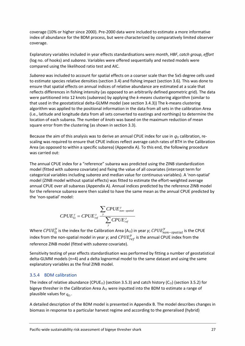
For q calibration runs, the shape parameter value is arbitrarily fixed at 0.4 ( K4.0=ϕ ) and the observation error ( oσ ) was fixed at 0.2. BDMs were fitted to the catch history (CΩ) and abundance index (CPUEΩ) for bigeye thresher in the Calibration Area, and to an informed prior on the maximum intrinsic population growth rate r for the species (lognormal with mean 0.03 and standard deviation 0.02) (section 3.7) (see Figure 4 for conceptual representation).
The population was unlikely to be in an unfished equilibrium state at the start of our time series in 1995 (i.e., initial depletion or initial stock status relative to the unfished biomass u <1). Because the initial depletion state could not be estimated by the model, a set of values u were randomly sampled from three normal distributions with means 0.3 (low initial status), 0.5 (medium initial status) and 0.7 (high initial status) and a standard deviation of 0.05. Each was sampled 300 times, for a total sample of 900 u values ranging from 0.15 to 0.84 (Figure 8). A BDM was fitted to each u to obtain 1000 posterior samples of q (total 3000 samples across the three u assumptions). The combined samples constitute the plausible range of q across the three initial stock status scenarios.
A uniform prior was assumed for K (unfished biomass at equilibrium) in log space (which serves to give lower probabilities to higher K values). Prior bounds were defined to constrain the estimates to biologically plausible values. The lower bound for K was set at 30 000 sharks, based on the estimated maximum annual catch in the Calibration Area. The upper bound was determined based on expert knowledge and advice on plausible values of bigeye thresher density in fishery hotspots. The base case scenario used an upper bound of 2 million sharks, which is the biomass (K) value corresponding to a ≤ 5% chance of encountering more than one shark per km2 in hotspots cells (i.e., cells 436, 437, and 438 - see Figure 11). This value was derived based on the combined surface area of the three cells (approximately 900 000 km2) and the fact that approximately 50% of the estimated density for the Calibration Area was located in those cells (see spatial standardisation results, section 4.1). As sensitivities, alternative values for the upper bound were considered based on estimates of K from the most recent assessment of blue shark in the North Pacific region (WCPFC 2014), however recognising that blue shark is a more productive species with potentially higher abundance. Alternative upper bound values were derived using two approaches: (1) by applying the ratio of the upper to lower bound of K for blue shark (= 200) to the maximum observed catch of bigeye thresher in the Calibration Area (30 000 sharks) (= 6 million upper bound); and (2) by using the best estimate of K for blue sharks in the North Pacific region (i.e., average of the median estimates from the four main reference models = 1.04 million tonnes (see Table 8 of WCPFC (2014)), corresponding to approximately 37 million sharks, assuming an average weight of 28 kg for blue shark caught in the longline fishery (Nakano 1994)). This number was scaled to the Calibration Area for bigeye thresher (using the results of the spatial standardisation in Section 3.4), to yield an upper bound of 16 million bigeye thresher.
This multiple scenario approach served to constrain the uncertainty in the estimated parameters, and ensure that q estimates derived from the calibration process reflect a range of biologically plausible values. This was required as the lack of contrast in the abundance index did not permit the BDM to estimate the upper range of the unfished biomass at equilibrium K.
The state-space estimation procedure implemented in BDM allows for the inclusion of process error. The value inputted for the process error standard deviation (0.05) was based on recommendations by McAllister (2013). Process error allows the model to account for inter-annual variability in stock
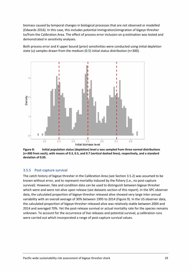
Pacific-wide sustainability risk assessment of bigeye thresher shark 29
biomass caused by temporal changes in biological processes that are not observed or modelled (Edwards 2016). In this case, this includes potential immigration/emigration of bigeye thresher to/from the Calibration Area. The effect of process error inclusion on q estimation was tested and demonstrated in sensitivity analyses.
Both process error and K upper bound (prior) sensitivities were conducted using initial depletion state (u) samples drawn from the medium (0.5) initial status distribution (n=300).
Figure 8: Initial population status (depletion) level u was sampled from three normal distributions (n=300 from each), with means of 0.3, 0.5, and 0.7 (vertical dashed lines), respectively, and a standard deviation of 0.05.
3.5.5 Post-capture survival The catch history of bigeye thresher in the Calibration Area (see Section 3.5.2) was assumed to be known without error, and to represent mortality induced by the fishery (i.e., no post-capture survival). However, fate and condition data can be used to distinguish between bigeye thresher which were and were not alive upon release (see datasets section of this report). In the SPC observer data, the calculated proportion of bigeye thresher released alive showed very large inter-annual variability with an overall average of 30% between 1995 to 2014 (Figure 9). In the US observer data, the calculated proportion of bigeye thresher released alive was relatively stable between 2004 and 2014 and averaged 70%. Yet the post-release survival or actual mortality rate for the species remains unknown. To account for the occurrence of live releases and potential survival, q calibration runs were carried out which incorporated a range of post-capture survival values.
30 Pacific-wide sustainability risk assessment of bigeye thresher shark
This required the catch vector (or annual harvest rate Ht) in the Calibration Area to be adjusted by applying an assumed post-capture survival rate s:
( )sHH tt −= 1'
where H’ is the annual harvest rate (ratio of catch over abundance) adjusted for post-capture survival. In each BDM run (and across the range of initial population status scenarios described above), s was randomly drawn from a uniform distribution with bounds [0.3, 0.7]. This range was loosely based on the calculated proportion of BTH released alive in the SPC and US observer datasets (Figure 9).
A similar adjustment of posterior estimates for q in the Calibration Area (qΩ) was necessary to propagate post-capture survival assumptions into fishing mortality estimation:
( )sqq −=ΩΩ
1'
Figure 9: Annual proportion of BTH released alive for US observer data 2003–2014 and SPC observer data 1995–2014
3.5.6 Spatial scaling and adjustments by fishery groups The catchability scalar was adjusted by fishery groups to account for differences in operational practices and associated capture efficiency for bigeye thresher among fishery sectors.
Fishery group-specific catchability jq was estimated as:
jj qfq =
Pacific-wide sustainability risk assessment of bigeye thresher shark 31
where q is the average population catchability (qΩ) scaled to the spatial resolution of the
assessment (5x5 degree cells) and jf is the adjustment factor for fishery group j (see Appendix C for complete derivation).
The adjustment factor jf was calculated as the predicted catch rate for each fishery group relative to a reference group (defined as the ‘BET’ catch group and ‘Jan-Mar’ season) using the final (spatial standardisation) ZINB model fitted to all observer data within the Core Area. Since month was modelled as a continuous variable, seasonal predictions were based on the intermediate month within each season (i.e., February for Jan-Mar).
Uncertainty in jf can be estimated using a bootstrap procedure (similar to that used for the spatial
abundance indices) but this was done in this assessment.
3.5.7 Key assumptions Our q estimation method assumes that the Calibration Area and US Hawaii observer data are representative of population dynamics for bigeye thresher sharks at the scale of the Pacific Ocean. This means we assume that on average the fishing power of longline sets on bigeye thresher is the same across the Pacific region, but differences in relative catchability (catch group and seasonal effects) and population density explain the differences in catch rates. This is unlikely to be the case but was a necessary assumption in the absence of informative data indicating otherwise. The assumptions made on the initial population status (low, median, and high) are arbitrary and intended to improve estimation and ensure realistic outcomes in q estimation. Indirectly, initial stock status assumptions also served to deal with uncertainty in post-capture survival of bigeye thresher in pelagic longline fisheries (e.g., a high post-capture survival scenario can be expected to result in a higher initial stock status, and vice-versa). As in most age-structured stock assessment models, values of q are assumed to remain constant over the time frame of the assessment (2000-2014).
3.6 Impact estimation (fishing mortality) Impact was estimated relative to the total (commercial) pelagic longline effort available in the CES Longline Logsheet dataset, from 2000 to 2014.
Spatially-explicit impact is the average annual fishing mortality in 5x5 degree cells calculated using commercial effort data (split by fishery groups), species relative density and fishery group catchability. We assumed cumulative fishing mortality as contributed from different fishery groups in each cell, and cumulative impact over the spatial domain of the assessment. Fishing mortality in each cell was calculated as the product of effort and fishery group catchability and contrasted across a range of scenarios (i.e., the three initial population status assumptions used to calibrate the catchability scalar and with and without taking into account the occurrence of post-capture survival). Since the catchability parameter was calibrated using a plausible range of K values with upper bound constrained based on expert opinion (or information from another species in sensitivity analyses), estimates of fishing mortality represent the plausible range of fishing mortality for the species over the timeframe of the assessment, as constrained by the available data and expert knowledge. Impacts were estimated for the Core Area (using species relative density estimates derived from the ZINB model) and the Assessment Area (using density estimates from the delta-GLMM model). Uncertainty in species distribution information is incorporated in impact estimation by resampling density indices from bootstrapped estimates.
32 Pacific-wide sustainability risk assessment of bigeye thresher shark
3.7 Population productivity and MIST estimation
3.7.1 Maximum intrinsic growth rate r The life history module (LHM) for BDM developed by Edwards (2016) was used to estimate a distribution for the maximum intrinsic population growth rate r for bigeye thresher. The model implements Monte Carlo sampling of life history parameter distributions, with iterated solving of the Euler-Lotka equation (McAllister et al. 2001). The Euler-Lotka equation defines maximum intrinsic growth r as the net balance of survivorship s and unconstrained fecundity f, integrated over all age classes a:
∑ safae-ar∞a=0 =1
sa=e-aM
fa=α mawa
Survivorship (s) is a function of the natural mortality M, assumed constant across ages. Fecundity (f) is the product of female maturity m, weight w and the maximum recruits per spawner α (in the absence of density dependent effects). The relevant functional forms are the maturity-at-age ma, length-at-age la (modelled as per von Bertalanffy growth), weight-at-age wa and recruits per spawner α:
ma=1+exp((a50-a) δ⁄ )-1
la=l∞ 1-exp-k(a-t0)
wa=alab
α=4h
ρ(1-h)
Recruits per spawner is related to steepness h and the female spawning biomass per recruit ρ, assuming a Beverton-Holt stock recruitment relationship. Current LHM parameterisation requires a value of h to be specified. The model incorporates uncertainty in all parameters, which can be fixed on input (for details see https://github.com/cttedwards/lhm). Maximum age Amax is treated as a single asymptotic value in the model. Steepness is modelled as a bounded beta distribution and all other life history parameters are modelled as random lognormal variables. Life history data used to estimate a distribution for r are summarized in Table 5. Parameter values calculated for females of bigeye thresher were used whenever possible. Parameters that were poorly-informed or unobserved (i.e., those relating to maturation and recruitment) were given a higher cv (0.2) in the estimation process, and others that were estimated based on observations with sample sizes >100 specimens (growth and longevity) were given a cv of 0.10. We assumed that females have a litter size of two (Chen et al. 1997) and an annual reproductive cycle.
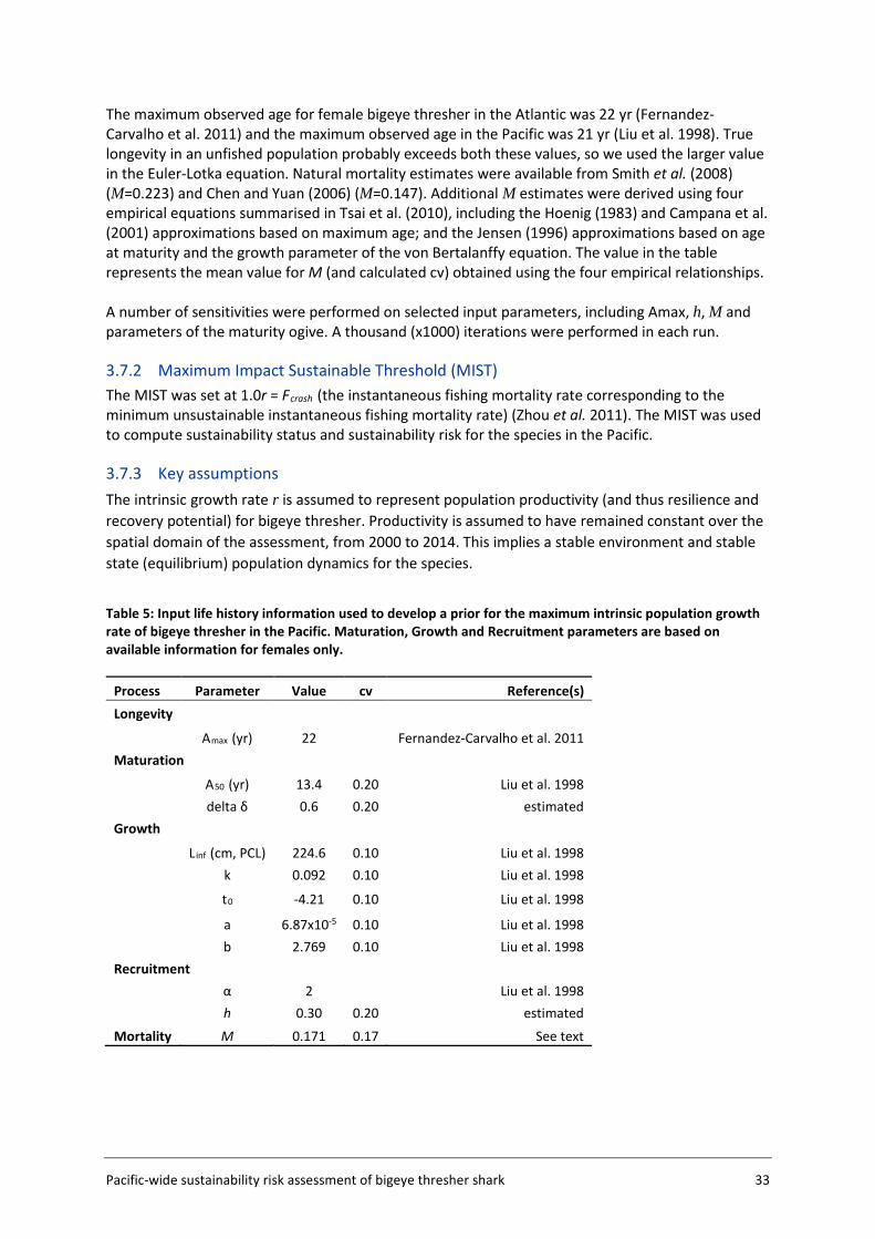
Pacific-wide sustainability risk assessment of bigeye thresher shark 33
The maximum observed age for female bigeye thresher in the Atlantic was 22 yr (Fernandez-Carvalho et al. 2011) and the maximum observed age in the Pacific was 21 yr (Liu et al. 1998). True longevity in an unfished population probably exceeds both these values, so we used the larger value in the Euler-Lotka equation. Natural mortality estimates were available from Smith et al. (2008) (M=0.223) and Chen and Yuan (2006) (M=0.147). Additional M estimates were derived using four empirical equations summarised in Tsai et al. (2010), including the Hoenig (1983) and Campana et al. (2001) approximations based on maximum age; and the Jensen (1996) approximations based on age at maturity and the growth parameter of the von Bertalanffy equation. The value in the table represents the mean value for M (and calculated cv) obtained using the four empirical relationships. A number of sensitivities were performed on selected input parameters, including Amax, h, M and parameters of the maturity ogive. A thousand (x1000) iterations were performed in each run.
3.7.2 Maximum Impact Sustainable Threshold (MIST) The MIST was set at 1.0r = Fcrash (the instantaneous fishing mortality rate corresponding to the minimum unsustainable instantaneous fishing mortality rate) (Zhou et al. 2011). The MIST was used to compute sustainability status and sustainability risk for the species in the Pacific.
3.7.3 Key assumptions The intrinsic growth rate r is assumed to represent population productivity (and thus resilience and recovery potential) for bigeye thresher. Productivity is assumed to have remained constant over the spatial domain of the assessment, from 2000 to 2014. This implies a stable environment and stable state (equilibrium) population dynamics for the species.
Table 5: Input life history information used to develop a prior for the maximum intrinsic population growth rate of bigeye thresher in the Pacific. Maturation, Growth and Recruitment parameters are based on available information for females only.
Process Parameter Value cv Reference(s) Longevity
Amax (yr) 22 Fernandez-Carvalho et al. 2011 Maturation
A50 (yr) 13.4 0.20 Liu et al. 1998
delta δ 0.6 0.20 estimated Growth
Linf (cm, PCL) 224.6 0.10 Liu et al. 1998
k 0.092 0.10 Liu et al. 1998
t0 -4.21 0.10 Liu et al. 1998
a 6.87x10⁻⁵ 0.10 Liu et al. 1998
b 2.769 0.10 Liu et al. 1998 Recruitment α 2 Liu et al. 1998
h 0.30 0.20 estimated Mortality M 0.171 0.17 See text
34 Pacific-wide sustainability risk assessment of bigeye thresher shark
3.8 Sustainability risk calculations Sustainability status was determined relative to fishing impact from pelagic longline fisheries in the Pacific over the period 2000-2014, and computed relative to a MIST=1.0r= Fcrash. A sustainability risk metric, corresponding to the ratio of total impact to the species MIST, was computed and compared between impact estimated at the scale of the Core Area (ZINB model species distribution) and impact estimated at the scale of the Assessment Area (delta-GLMM model species distribution). The probability that current impacts exceed the MIST (Pr(Impact/MIST>1)) was calculated by re-sampling across the uncertainty range estimated for all parameters. Additional sustainability risk thresholds were defined a posteriori based on the distribution of annual sustainability status and uncertainty.
4 ASSESSMENT RESULTS Characteristics of the observer data (and observer data coverage) relevant to the assessment are presented in Appendix D. Owing to the complexity and multiple dimensions of this assessment, the following sections were structured to describe the main results of key components, namely species distribution, catchability, fishing impact and sustainability status and risk. Details on multiple model fitting, assumptions, sensitivities and comparisons, are presented in the appendices and referred to as appropriate in the text.
4.1 Species distribution The estimated spatial distribution for bigeye thresher using the final ZINB model (Core Area distribution) and the spatial delta-GLMM model (Assessment Area distribution) are mapped in Figure 10. Abundance ‘hot spots’ and predicted densities (spatial indices of relative abundance) in Core Area cells were similar between the two models (Figure 11). Highest densities occurred between latitude 5°N and 15°N and, according to the extrapolated distribution from the delta-GLMM model, spanned a broad longitudinal range from 150°E to approximately 140°W (220°E on map).
The three delta-GLMM models predicted similar, highest densities within three adjacent cells (cell ID 438, 437 and 436 – see Figure 5), which demonstrates the smoothing effect of the spatial correlation (Figures 10, 11). ZINB outputs were patchier and predicted a higher relative density in cell ID 438 and a lower density in cell ID 436. Encounter probabilities were highly variable among cells and ranged from 2% to 72% within the Core Area. Predicted catch rates per cell (no. of captures per 1000 hooks) were generally less than 2.
The final ZINB model included cell_ID, year, month, catch group and HBF as significant covariates (Appendix E). Effort (no. of hooks) was included as an offset term to predict relative densities as the number of captures per 1000 hooks in 5x5 degree cells. Relationships between explanatory variables and encounter probabilities and catch rates were generally weak, suggesting that spatial effects explained most of the variation in catch rates of bigeye thresher within the Core Area.
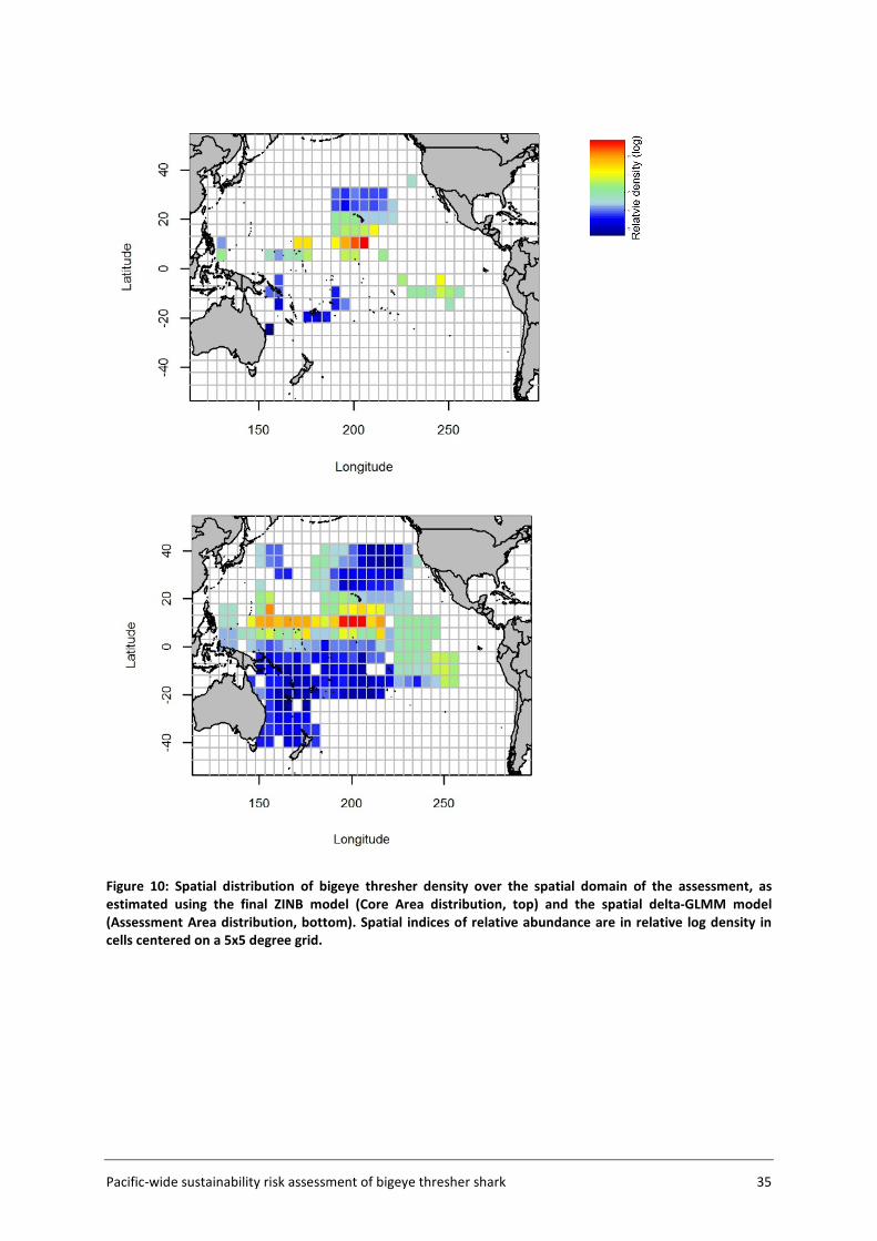
Pacific-wide sustainability risk assessment of bigeye thresher shark 35
Figure 10: Spatial distribution of bigeye thresher density over the spatial domain of the assessment, as estimated using the final ZINB model (Core Area distribution, top) and the spatial delta-GLMM model (Assessment Area distribution, bottom). Spatial indices of relative abundance are in relative log density in cells centered on a 5x5 degree grid.
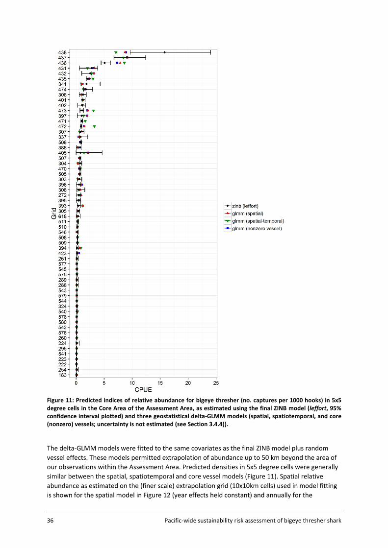
36 Pacific-wide sustainability risk assessment of bigeye thresher shark
Figure 11: Predicted indices of relative abundance for bigeye thresher (no. captures per 1000 hooks) in 5x5 degree cells in the Core Area of the Assessment Area, as estimated using the final ZINB model (leffort, 95% confidence interval plotted) and three geostatistical delta-GLMM models (spatial, spatiotemporal, and core (nonzero) vessels; uncertainty is not estimated (see Section 3.4.4)).
The delta-GLMM models were fitted to the same covariates as the final ZINB model plus random vessel effects. These models permitted extrapolation of abundance up to 50 km beyond the area of our observations within the Assessment Area. Predicted densities in 5x5 degree cells were generally similar between the spatial, spatiotemporal and core vessel models (Figure 11). Spatial relative abundance as estimated on the (finer scale) extrapolation grid (10x10km cells) used in model fitting is shown for the spatial model in Figure 12 (year effects held constant) and annually for the
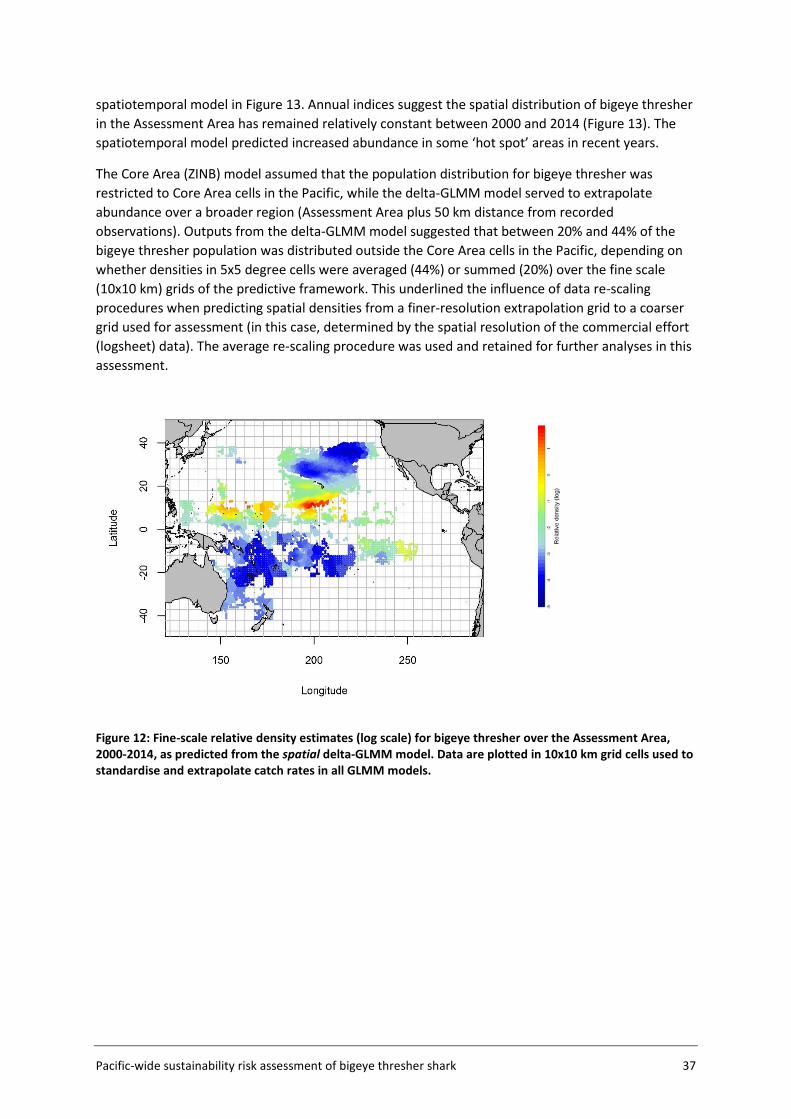
Pacific-wide sustainability risk assessment of bigeye thresher shark 37
spatiotemporal model in Figure 13. Annual indices suggest the spatial distribution of bigeye thresher in the Assessment Area has remained relatively constant between 2000 and 2014 (Figure 13). The spatiotemporal model predicted increased abundance in some ‘hot spot’ areas in recent years.
The Core Area (ZINB) model assumed that the population distribution for bigeye thresher was restricted to Core Area cells in the Pacific, while the delta-GLMM model served to extrapolate abundance over a broader region (Assessment Area plus 50 km distance from recorded observations). Outputs from the delta-GLMM model suggested that between 20% and 44% of the bigeye thresher population was distributed outside the Core Area cells in the Pacific, depending on whether densities in 5x5 degree cells were averaged (44%) or summed (20%) over the fine scale (10x10 km) grids of the predictive framework. This underlined the influence of data re-scaling procedures when predicting spatial densities from a finer-resolution extrapolation grid to a coarser grid used for assessment (in this case, determined by the spatial resolution of the commercial effort (logsheet) data). The average re-scaling procedure was used and retained for further analyses in this assessment.
Figure 12: Fine-scale relative density estimates (log scale) for bigeye thresher over the Assessment Area, 2000-2014, as predicted from the spatial delta-GLMM model. Data are plotted in 10x10 km grid cells used to standardise and extrapolate catch rates in all GLMM models.
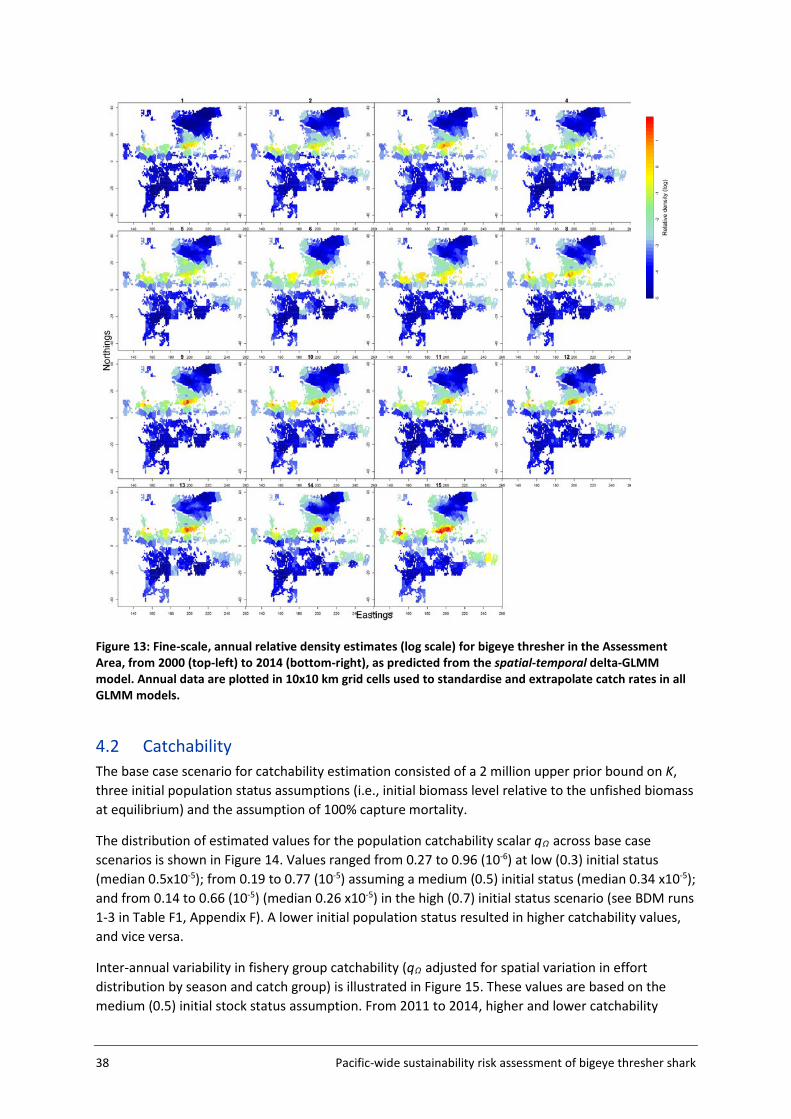
38 Pacific-wide sustainability risk assessment of bigeye thresher shark
Figure 13: Fine-scale, annual relative density estimates (log scale) for bigeye thresher in the Assessment Area, from 2000 (top-left) to 2014 (bottom-right), as predicted from the spatial-temporal delta-GLMM model. Annual data are plotted in 10x10 km grid cells used to standardise and extrapolate catch rates in all GLMM models.
4.2 Catchability The base case scenario for catchability estimation consisted of a 2 million upper prior bound on K, three initial population status assumptions (i.e., initial biomass level relative to the unfished biomass at equilibrium) and the assumption of 100% capture mortality.
The distribution of estimated values for the population catchability scalar qΩ across base case scenarios is shown in Figure 14. Values ranged from 0.27 to 0.96 (10-6) at low (0.3) initial status (median 0.5x10⁻⁵); from 0.19 to 0.77 (10-5) assuming a medium (0.5) initial status (median 0.34 x10⁻⁵); and from 0.14 to 0.66 (10-5) (median 0.26 x10⁻⁵) in the high (0.7) initial status scenario (see BDM runs 1-3 in Table F1, Appendix F). A lower initial population status resulted in higher catchability values, and vice versa.
Inter-annual variability in fishery group catchability (qΩ adjusted for spatial variation in effort distribution by season and catch group) is illustrated in Figure 15. These values are based on the medium (0.5) initial stock status assumption. From 2011 to 2014, higher and lower catchability
Pacific-wide sustainability risk assessment of bigeye thresher shark 39
characterised the Apr-Jun/Oct-Dec and Jan-Mar/Jul-Sep seasons, respectively. Effort mainly catching SWO had comparatively lower (and a narrower range of) catchability. Higher catchability characterised the fleet that mainly caught bigeye tuna (BET) in each year. Other catch groups showed intermediate and generally variable catchability values. A summary of inter-annual variability in fishery groups catchability by year, catch group and season, for the period 2000-2014, is presented in Tables F2 and F3 of Appendix F.
Figure 14: Estimated distributions of the catchability scalarΩq for each initial stock status (biomass level
relative to the unfished biomass at equilibrium) assumption (low=0.3; medium=0.5 and high=0.7) considered in BDM calibration (BDM run 1-3 in Table F1, Appendix F). Assuming a range of post-capture survival rates produced median catchability estimates that were 32-35% lower than the 100% capture mortality scenarios (run 1s-3s in Table F1, Appendix F). Increasing the upper bound value of the K prior likewise resulted in lower catchability estimates (runs 2a and 2b in Table F1, Appendix F). The calibration model was sensitive to the inclusion of process error, which permitted fitting the index of relative abundance without over-estimating the unobserved biomass state (Appendix F).
40 Pacific-wide sustainability risk assessment of bigeye thresher shark
(a)
(b)
Figure 15: Distributions of estimated catchability q by year and fishery groups disaggregated by (a) fishing season and (b) catch group. Values are based on the distribution for Ωq derived assuming a medium (0.5) initial biomass level for the stock.
The catch history (assuming 100% capture mortality) and standardised CPUE index of abundance used in BDM calibrations are shown in Figure 16 and Figure 17, respectively. Annual CPUE indices are tabulated (with 95% confidence intervals) in Table 6. Time series of estimated depletion and predicted abundance indices for the base-case scenarios are given in Appendix F (Figure F1). The CPUE index of abundance was not informative of stock status as the model was able to fit the trend in the CPUE indices by varying initial status assumptions. This is because the standardised CPUE index lacked contrast and was inconsistent with the derived catch series (i.e., the presence of trends in some parts of the CPUE series, including a substantial decline from 1996 to 2000 and a slight increase through the early 2000s, were not well explained by the catch history). This did not permit the biomass dynamic model to infer stock status by interpreting changes in relative abundance in
Pacific-wide sustainability risk assessment of bigeye thresher shark 41
response to the harvest. Re-constructed catches between 2000 and 2014 were similar among stratifications but differed in some years prior to 2000 (Figure 16). This may or may not be related to comparatively limited observer coverage over the 1995-2000 period. The complete catch series and detailed information on observer and commercial effort data used to derive catch estimates for BTH in the Calibration Area are given in Appendix G.
Figure 16: Estimated catch (1995-2014) and approximated catch history (1952-1994) for BTH within the Calibration Area. Catch estimates for 1995−2014 are compared among stratification methods. The catch history for 1952−1994 is shown for comparison but was not used for analyses. The standardised CPUE indices of abundance predicted using different models showed a consistent trend over time. Explanatory variables included in the final ZINB (and other) models were year, month, catch group, subarea, HBF and effort (log no. of hooks). Subarea had a large influence in determining the annual trend (the trend in annual indices changed very little when other variables were offered). Important fluctuations and higher variability early in the time series probably reflect comparatively limited effort and/or observer coverage. Changes in fishing patterns over time were evidenced in coefficient-distribution influence plots (Bentley et al. 2012) for explanatory variables in the delta lognormal model (Figure 18). Numbers of shallow sets (low HBFs) were higher in 1995-1997 and decreased thereafter. Effort mainly catching ALB was reduced in 2002-2014 compared to 1995-2001. The slight increasing trend from 2000 onwards can be partly explained by an increase in observed effort in subareas that have lower catch rates during this period (i.e., in the standardisation model, catch rates are dependent on year, subarea, and other factors in a multiplicative manner. Thus, everything else being equal, subareas with lower effects probably served to push the standardised year effects higher, and vice versa (see Figure 18)).
The nominal CPUE in 2014 was more than twice that in 2013. The reason for this is not clear, although further investigation suggested most of the increase in catch occurred in one cell (cell_ID 436), where a gradual increase in effort has also occurred over the last five years. In addition, over a third of catch in 2014 was taken in May, which had the highest SST among the last 8 years. A sensitivity model that removed the 2014 data did not change the overall abundance trend (Appendix H), consistent with the results of a similar sensitivity test on these data (Young et al. 2016). Detailed results, model diagnostics and additional sensitivities performed in the development of a CPUE index of abundance for bigeye thresher in the Calibration Area are presented in Appendix H.
42 Pacific-wide sustainability risk assessment of bigeye thresher shark
Figure 17: Annual CPUE indices of relative abundance (mean and 95% CI) for bigeye thresher in the Calibration Area, 1995-2014, predicted using (a) the final ZINB model and the delta-GLMM model fitted with 1000 knots; and b) the final ZINB model, the same ZINB model excluding year 2014, and a delta lognormal GLM model. All models were fitted to US Hawaii observer data from the Calibration Area. Grey dots in (b) are nominal (unstandardised) CPUE. All indices were normalised to the mean of each series to allow comparison.
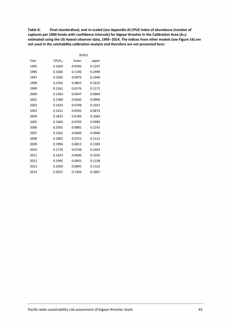
Pacific-wide sustainability risk assessment of bigeye thresher shark 43
Table 6: Final standardised, and re-scaled (see Appendix A) CPUE index of abundance (number of captures per 1000 hooks with confidence intervals) for bigeye thresher in the Calibration Area (AΩ) estimated using the US Hawaii observer data, 1995−2014. The indices from other models (see Figure 16) are not used in the catchability calibration analysis and therefore are not presented here.
95%CI
Year CPUEΩ lower upper
1995 0.1664 0.0596 0.1247
1996 0.3260 0.1196 0.2490
1997 0.2585 0.0979 0.1949
1998 0.2356 0.0855 0.1610
1999 0.1561 0.0176 0.1171
2000 0.1364 0.0447 0.0904
2001 0.1390 0.0560 0.0904
2002 0.1633 0.0708 0.1037
2003 0.1421 0.0595 0.0874
2004 0.1833 0.0784 0.1064
2005 0.1660 0.0704 0.0989
2006 0.2055 0.0881 0.1242
2007 0.1562 0.0669 0.0946
2008 0.1805 0.0753 0.1111
2009 0.1994 0.0813 0.1309
2010 0.1776 0.0738 0.1093
2011 0.1623 0.0690 0.1020
2012 0.1995 0.0855 0.1238
2013 0.2050 0.0845 0.1322
2014 0.3027 0.1304 0.1867
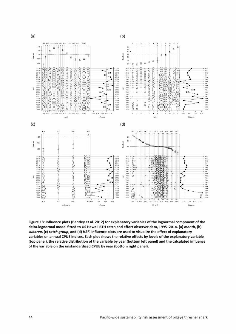
44 Pacific-wide sustainability risk assessment of bigeye thresher shark
(a)
(b)
(c)
(d)
Figure 18: Influence plots (Bentley et al. 2012) for explanatory variables of the lognormal component of the delta-lognormal model fitted to US Hawaii BTH catch and effort observer data, 1995–2014. (a) month, (b) subarea, (c) catch group, and (d) HBF. Influence plots are used to visualize the effect of explanatory variables on annual CPUE indices. Each plot shows the relative effects by levels of the explanatory variable (top panel), the relative distribution of the variable by year (bottom left panel) and the calculated influence of the variable on the unstandardized CPUE by year (bottom right panel).
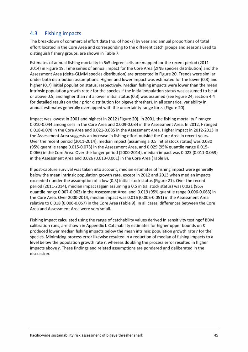
Pacific-wide sustainability risk assessment of bigeye thresher shark 45
4.3 Fishing impacts The breakdown of commercial effort data (no. of hooks) by year and annual proportions of total effort located in the Core Area and corresponding to the different catch groups and seasons used to distinguish fishery groups, are shown in Table 7.
Estimates of annual fishing mortality in 5x5 degree cells are mapped for the recent period (2011-2014) in Figure 19. Time series of annual impact for the Core Area (ZINB species distribution) and the Assessment Area (delta-GLMM species distribution) are presented in Figure 20. Trends were similar under both distribution assumptions. Higher and lower impact was estimated for the lower (0.3) and higher (0.7) initial population status, respectively. Median fishing impacts were lower than the mean intrinsic population growth rate r for the species if the initial population status was assumed to be at or above 0.5, and higher than r if a lower initial status (0.3) was assumed (see Figure 24, section 4.4 for detailed results on the r prior distribution for bigeye thresher). In all scenarios, variability in annual estimates generally overlapped with the uncertainty range for r. (Figure 20). Impact was lowest in 2001 and highest in 2012 (Figure 20). In 2001, the fishing mortality F ranged 0.010-0.044 among cells in the Core Area and 0.009-0.034 in the Assessment Area. In 2012, F ranged 0.018-0.078 in the Core Area and 0.021-0.085 in the Assessment Area. Higher impact in 2012-2013 in the Assessment Area suggests an increase in fishing effort outside the Core Area in recent years. Over the recent period (2011-2014), median impact (assuming a 0.5 initial stock status) was 0.030 (95% quantile range 0.015-0.073) in the Assessment Area, and 0.029 (95% quantile range 0.015-0.066) in the Core Area. Over the longer period (2000-2014), median impact was 0.023 (0.011-0.059) in the Assessment Area and 0.026 (0.013-0.061) in the Core Area (Table 8). If post-capture survival was taken into account, median estimates of fishing impact were generally below the mean intrinsic population growth rate, except in 2012 and 2013 when median impacts exceeded r under the assumption of a low (0.3) initial stock status (Figure 21). Over the recent period (2011-2014), median impact (again assuming a 0.5 initial stock status) was 0.021 (95% quantile range 0.007-0.063) in the Assessment Area, and 0.019 (95% quantile range 0.006-0.063) in the Core Area. Over 2000-2014, median impact was 0.016 (0.005-0.051) in the Assessment Area relative to 0.018 (0.006-0.057) in the Core Area (Table 9). In all cases, differences between the Core Area and Assessment Area were very small. Fishing impact calculated using the range of catchability values derived in sensitivity testingof BDM calibration runs, are shown in Appendix I. Catchability estimates for higher upper bounds on K produced lower median fishing impacts below the mean intrinsic population growth rate r for the species. Minimizing process error likewise resulted in a reduction of median of fishing impacts to a level below the population growth rate r, whereas doubling the process error resulted in higher impacts above r. These findings and related assumptions are pondered and deliberated in the discussion.
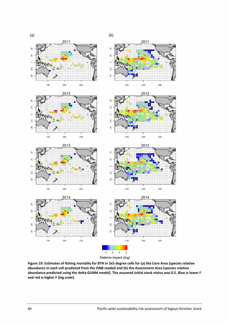
46 Pacific-wide sustainability risk assessment of bigeye thresher shark
(a)
(b)
Figure 19: Estimates of fishing mortality for BTH in 5x5 degree cells for (a) the Core Area (species relative abundance in each cell predicted from the ZINB model) and (b) the Assessment Area (species relative abundance predicted using the delta-GLMM model). The assumed initial stock status was 0.5. Blue is lower F and red is higher F (log scale).
Pacific-wide sustainability risk assessment of bigeye thresher shark 47
Table 7: Summary of commercial (pelagic longline) effort information used to estimate fishing impact for bigeye thresher in the Pacific Ocean. Total number of hooks by year and percentages (%) of total effort within the Core Area, and corresponding to each of the catch groups and seasons used to differentiate fishery groups.
Total hooks Core Area Catch group (%) Season (%)
Year (millions) (%) YFT ALB BET SWO Others Jan–Mar Apr–Jun Jul–Sep Oct–Dec
2000 507 25.69 26.95 22.88 48.35 1.82 <0.01 25.18 23.63 27.14 24.05
2001 574 24.90 26.14 23.86 48.91 1.08 <0.01 27.13 23.31 25.38 24.19
2002 681 26.63 19.15 27.68 52.40 0.77 <0.01 24.53 21.69 27.91 25.86
2003 711 32.34 23.27 26.11 49.84 0.78 <0.01 23.47 24.80 26.13 25.60
2004 681 26.00 16.18 27.80 55.22 0.79 <0.01 25.02 22.47 26.44 26.07
2005 614 30.39 15.61 33.72 49.98 0.69 <0.01 25.66 23.40 26.70 24.23
2006 607 32.26 15.94 36.01 47.35 0.71 <0.01 22.71 25.56 26.88 24.85
2007 599 31.19 19.89 32.49 46.02 1.59 <0.01 23.74 23.96 27.30 25.00
2008 610 30.55 16.75 33.41 48.53 1.26 0.04 23.55 25.64 25.82 24.99
2009 647 27.22 19.73 38.88 39.53 1.86 0.01 23.11 24.99 27.31 24.59
2010 676 28.84 18.62 41.45 38.17 1.75 0.02 22.60 24.63 27.45 25.32
2011 730 30.69 23.05 36.62 38.43 1.85 0.05 22.79 24.50 25.44 27.28
2012 776 28.19 15.10 43.20 40.16 1.53 0.01 24.24 25.73 24.96 25.08
2013 729 31.04 18.74 45.37 35.14 0.74 0.00 24.57 28.02 26.31 21.11
2014 649 32.13 23.36 40.91 34.77 0.94 0.02 22.34 26.33 26.53 24.80
48 Pacific-wide sustainability risk assessment of bigeye thresher shark
(a)
(b)
Figure 20: Annual impact (median values and 95% quantile range) estimated for (a) the Core Area and (b) the Assessment Area, using catchability estimates derived assuming 100% post-capture mortality and three initial population status assumptions (low (0.3), medium (0.5), and high (0.7)) (BDM runs 1, 2, 3 from Table F1, Appendix F). The dashed line is the mean value for the estimated r prior (0.03), with 95% quantile range grey band (see section 4.4 for details).
(a)
(b)
Figure 21: Annual impact (median values and 95% quantile range) estimated for (a) the Core Area and (b) the Assessment Area, using catchability estimates adjusted for the occurrence of post-capture survival (random occurrence between 0.3 and 0.7) and assuming three initial population status assumptions (low (0.3), medium (0.5), and high (0.7)) (BDM run 1s, 2s, 3s from Table F1, Appendix F). The dashed line is the mean value for the estimated r prior (0.03), with 95% quantile range (grey band) (see section 4.4 for details).
Pacific-wide sustainability risk assessment of bigeye thresher shark 49
Table 8: Total impact (median F and 95% quantile range among cells) for the fifteen year period (2000-2014) and the recent period (2011-2014) in the Core Area and the Assessment Area, estimated assuming 100% post-capture mortality and three initial population status assumption (low (0.3), medium (0.5) and high (0.7)).
Impact Impact Impact
Low (0.3) Medium (0.5) High (0.7)
Core Area
2000-2014 0.038 (0.02-0.076) 0.026 (0.013-0.061) 0.019 (0.01-0.05)
2011-2014 0.042 (0.023-0.084) 0.029 (0.015-0.066) 0.022 (0.011-0.055) Assessment Area
2000-2014 0.034 (0.016-0.078) 0.023 (0.011-0.059) 0.018 (0.008-0.049)
2011-2014 0.044 (0.021-0.096) 0.03 (0.015-0.073) 0.023 (0.011-0.061)
Table 9: Total impact (median F and 95% quantile range among cells) for the fifteen year period (2000-2014) and the recent period (2011-2014) in the Core Area and the Assessment Area, estimated assuming the occurrence of post-capture survival (random occurrence between 0.3 and 0.7) and three initial population status assumptions (low (0.3), medium (0.5) and high (0.7)) (BDM run 1s, 2s, 3s from Table F1, Appendix F).
Impact Impact Impact
Low (0.3) Medium (0.5) High (0.7)
Core Area
2000-2014 0.025 (0.009-0.066) 0.018 (0.006-0.057) 0.014 (0.004-0.048)
2011-2014 0.028 (0.01-0.073) 0.019 (0.006-0.063 0.015 (0.005-0.052)
Assessment Area
2000-2014 0.024 (0.008-0.065) 0.016 (0.005-0.051) 0.012 (0.004-0.045)
2011-2014 0.03 (0.011-0.081) 0.021 (0.007-0.063) 0.015 (0.005-0.055)
Fishery group contributions to annual impact over the recent period (2011-2014) indicated a lower fishing mortality in Jul-Sep of each year in both the Core Area and Assessment Area, and higher fishing mortality in Apr-Jun (Figure 22). In 2011, a higher F was associated with the Oct-Dec season in the Core Area. Fishing mortality was highest in the BET catch group in all years, while the SWO fleet contributed minimal impact (Figure 23). Higher impact in 2012-2013 in the Assessment Area was linked to comparatively higher F contributions from the YFT fleet and the BET fleet during the Jan-Mar season.
50 Pacific-wide sustainability risk assessment of bigeye thresher shark
(a)
(b)
Figure 22: Annual fishing mortality (2011−2014) as contributed from different fishery groups (here distinguished by season) over (a) the Core Area and (b) the Assessment Area. Values are based on the medium (0.5) initial biomass level assumption.
(a)
(b)
Figure 23: Annual fishing mortality (2011−2014) as contributed from different fishery groups (here distinguished by catch group) over (a) the Core Area and (b) the Assessment Area. Values are based on the medium (0.5) initial biomass level assumption.
4.4 Sustainability risk The estimated distribution of the maximum intrinsic population growth rate r for bigeye thresher is shown in Figure 24. The distribution had a median 0.028 and cv 0.53 (Table 10). Results of sensitivity analyses indicated that the r estimation method used this study was most sensitive to recruitment assumptions relating to steepness (and associated maximum recruits per spawner). Decreasing the maximum annual number of recruits per spawner to less than 2 (in this case, 1.7 and 0.9) reduced median r values to 0.02 and 0.01, respectively, with increased variability (calculated cv=0.95 for r distribution estimated assuming α=0.9) (Table 10).
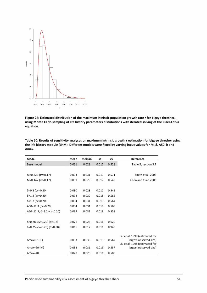
Pacific-wide sustainability risk assessment of bigeye thresher shark 51
Figure 24: Estimated distribution of the maximum intrinsic population growth rate r for bigeye thresher, using Monte Carlo sampling of life history parameters distributions with iterated solving of the Euler-Lotka equation.
Table 10: Results of sensitivity analyses on maximum intrinsic growth r estimation for bigeye thresher using the life history module (LHM). Different models were fitted by varying input values for M, δ, A50, h and Amax.
Model mean median sd cv Reference
Base model 0.031 0.028 0.017 0.528 Table 5, section 3.7
M=0.223 (cv=0.17) 0.033 0.031 0.019 0.571 Smith et al. 2008
M=0.147 (cv=0.17) 0.031 0.029 0.017 0.543 Chen and Yuan 2006
δ=0.3 (cv=0.20) 0.030 0.028 0.017 0.545 δ=1.2 (cv=0.20) 0.032 0.030 0.018 0.563 δ=1.7 (cv=0.20) 0.034 0.031 0.019 0.564 A50=12.3 (cv=0.20) 0.034 0.031 0.019 0.566 A50=12.3, δ=1.2 (cv=0.20) 0.033 0.031 0.019 0.558
h=0.28 (cv=0.20) (α=1.7) 0.026 0.023 0.016 0.620 h=0.25 (cv=0.20) (α=0.88) 0.016 0.012 0.016 0.945
Amax=21 (F) 0.033 0.030 0.019 0.567 Liu et al. 1998 (estimated for
largest observed size)
Amax=20 (M) 0.033 0.031 0.019 0.557 Liu et al. 1998 (estimated for
largest observed size)
Amax=40 0.028 0.025 0.016 0.585
52 Pacific-wide sustainability risk assessment of bigeye thresher shark
The estimated r distribution is taken to represent the maximum impact sustainable threshold (MIST) for the species, corresponding to the minimum unsustainable instantaneous fishing mortality rate (r = MIST =Fcrash) for the stock. Assuming 100% capture mortality, sustainability risk (ratio of impact to MIST) ranged from 0.6 to 1.2 in the Core Area (median values among initial population status assumptions) and between 0.6 and 1.1 in the Assessment Area, over the entire (2000-2014) assessment period (Figure 25, Table 11). For the recent period (2011-2014), sustainability risk ranged from 0.7 to 1.3 in the Core Area and from 0.7 to 1.4 in the Assessment Area. Sustainability risk was highest (and generally close to 1) under the assumption of a lower initial stock status for the species in the Pacific, and lower if initial status was assumed to be high. Accounting for post-capture survival reduced sustainability risk in all scenarios (range 0.4-0.8 for 2000-2014 in both the Core Area and Assessment Area) (Figure 25, Table 12). There was considerable uncertainty about sustainability risk. The upper range estimates (95% quantile) were above 1 in all scenarios, indicating the possibility that total impact from pelagic longline fisheries in the Pacific exceeded the minimum unsustainable fishing mortality rate for the species. Assuming 100% capture mortality, the calculated probability that the annual impact exceeded the MIST, given the uncertainty, averaged 0.4 and ranged 0.1-0.7 among years and distribution scenarios (Table 13). If post-capture survival was taken into account, the probability that the annual impact exceeded the MIST ranged from 0.1 to0.4 and averaged 0.2 (Table 13). Sustainability risk was generally stable among years and showed no directional trend over time, aside from a small increase in risk ratio over the recent period in the Assessment Area (Figure 25b). The probability that total impact exceeded the MIST was higher in the Assessment Area relative to the Core Area in 2012 and 2013. In other years, sustainability risk probabilities were higher in the Core Area (Table 13). Table 11 : Sustainability risk (ratio of impact to MIST with values >1 considered to be unsustainable) (median values and 95% quantile range) for bigeye thresher in the Pacific, as estimated for the Core Area and the Assessment Area assuming 100% capture mortality in impact estimation and three initial population status assumptions (low (0.3), medium (0.5), and high (0.7)). Results are contrasted for the fifteen year period (2000-2014) and the recent period (2011-2014).
Impact/MIST Impact/MIST Impact/MIST
Low (0.3) Medium (0.5) High (0.7)
Core Area
2000-2014 1.218 (0.527-3.05) 0.834 (0.349-2.357) 0.624 (0.252-1.883)
2011-2014 1.334 (0.597-3.253) 0.922 (0.385-2.537) 0.701 (0.292-2.052)
Assessment Area
2000-2014 1.076 (0.434-3.002) 0.746 (0.291-2.239) 0.567 (0.216-1.875)
2011-2014 1.387 (0.576-3.657) 0.959 (0.386-2.775) 0.733 (0.283-2.325)
Pacific-wide sustainability risk assessment of bigeye thresher shark 53
Table 12: Sustainability risk (ratio of impact to MIST with values >1 considered to be unsustainable) (median values and 95% quantile range) for bigeye thresher in the Pacific, as estimated for the Core Area and the Assessment Area assuming the occurrence of post-capture survival (random occurrence between 30% and 70%) in impact estimation and three initial population status assumptions (low (0.3), medium (0.5), and high (0.7)). Results are contrasted for the fifteen year period (2000-2014) and the recent period (2011-2014).
Impact/MIST Impact/MIST Impact/MIST
Low (0.3) Medium (0.5) High (0.7)
Core Area
2000-2014 0.815 (0.247-2.54) 0.563 (0.164-2.154) 0.438 (0.119-1.764)
2011-2014 0.902 (0.281-2.794) 0.619 (0.184-2.399) 0.483 (0.134-1.961)
Assessment Area
2000-2014 0.755 (0.23-2.426) 0.519 (0.148-1.89) 0.379 (0.11-1.62)
2011-2014 0.974 (0.302-3.051) 0.677 (0.193-2.428) 0.488 (0.142-2.065)
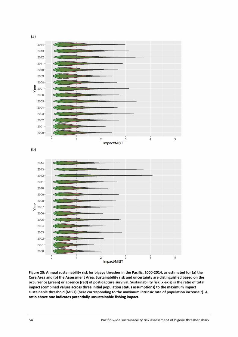
54 Pacific-wide sustainability risk assessment of bigeye thresher shark
(a)
(b)
Figure 25: Annual sustainability risk for bigeye thresher in the Pacific, 2000-2014, as estimated for (a) the Core Area and (b) the Assessment Area. Sustainability risk and uncertainty are distinguished based on the occurrence (green) or absence (red) of post-capture survival. Sustainability risk (x-axis) is the ratio of total impact (combined values across three initial population status assumptions) to the maximum impact sustainable threshold (MIST) (here corresponding to the maximum intrinsic rate of population increase r). A ratio above one indicates potentially unsustainable fishing impact.
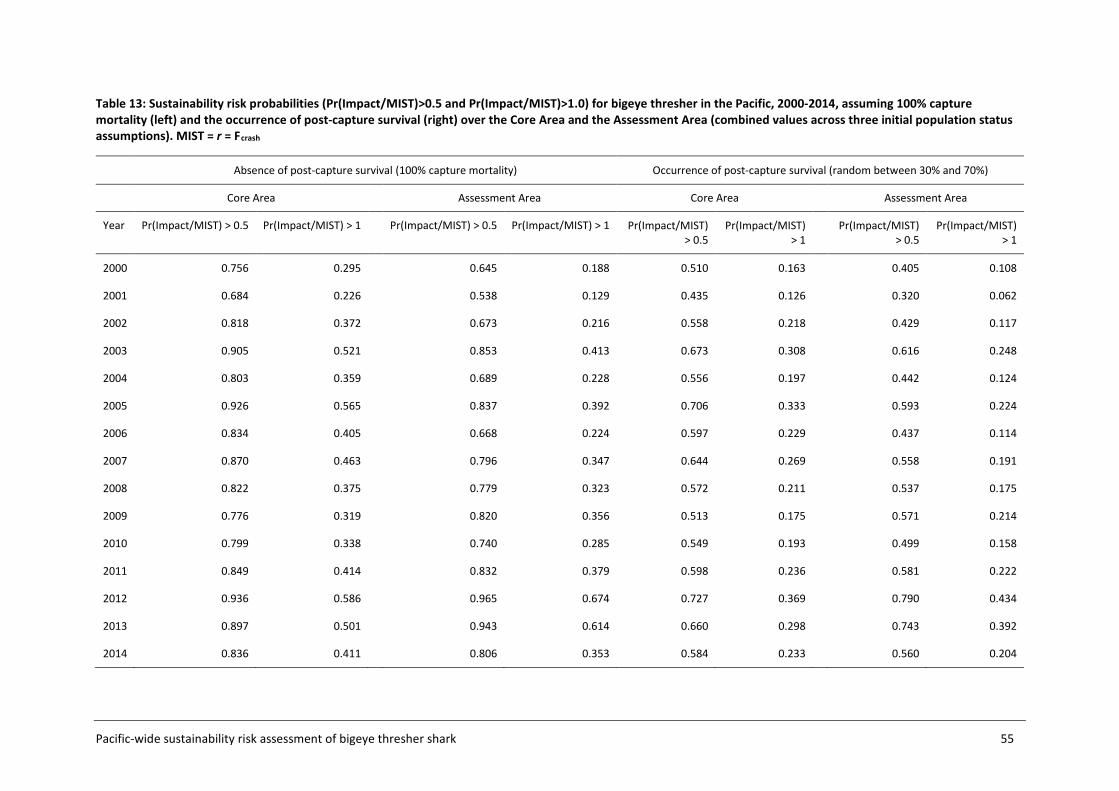
Pacific-wide sustainability risk assessment of bigeye thresher shark 55
Table 13: Sustainability risk probabilities (Pr(Impact/MIST)>0.5 and Pr(Impact/MIST)>1.0) for bigeye thresher in the Pacific, 2000-2014, assuming 100% capture mortality (left) and the occurrence of post-capture survival (right) over the Core Area and the Assessment Area (combined values across three initial population status assumptions). MIST = r = Fcrash
Absence of post-capture survival (100% capture mortality) Occurrence of post-capture survival (random between 30% and 70%)
Core Area Assessment Area Core Area Assessment Area
Year Pr(Impact/MIST) > 0.5 Pr(Impact/MIST) > 1
Pr(Impact/MIST) > 0.5 Pr(Impact/MIST) > 1 Pr(Impact/MIST) > 0.5
Pr(Impact/MIST) > 1
Pr(Impact/MIST) > 0.5
Pr(Impact/MIST) > 1
2000 0.756 0.295 0.645 0.188 0.510 0.163 0.405 0.108
2001 0.684 0.226 0.538 0.129 0.435 0.126 0.320 0.062
2002 0.818 0.372 0.673 0.216 0.558 0.218 0.429 0.117
2003 0.905 0.521 0.853 0.413 0.673 0.308 0.616 0.248
2004 0.803 0.359 0.689 0.228 0.556 0.197 0.442 0.124
2005 0.926 0.565 0.837 0.392 0.706 0.333 0.593 0.224
2006 0.834 0.405 0.668 0.224 0.597 0.229 0.437 0.114
2007 0.870 0.463 0.796 0.347 0.644 0.269 0.558 0.191
2008 0.822 0.375 0.779 0.323 0.572 0.211 0.537 0.175
2009 0.776 0.319 0.820 0.356 0.513 0.175 0.571 0.214
2010 0.799 0.338 0.740 0.285 0.549 0.193 0.499 0.158
2011 0.849 0.414 0.832 0.379 0.598 0.236 0.581 0.222
2012 0.936 0.586 0.965 0.674 0.727 0.369 0.790 0.434
2013 0.897 0.501 0.943 0.614 0.660 0.298 0.743 0.392
2014 0.836 0.411 0.806 0.353 0.584 0.233 0.560 0.204
56 Pacific-wide sustainability risk assessment of bigeye thresher shark
5 DISCUSSION AND RECOMMENDATIONS The assessment of fishing effects on pelagic sharks is complicated by limited data, inaccurate and incomplete catch records, and changes in fishing practices, reporting requirements and observer coverage over time. In thresher sharks, additional complexity arises from species identification problems leading to the grouping of three species (bigeye, common and pelagic thresher) into a single gender/species complex (Alopias or Thresher spp.) in commercial catch reports (logsheet data). Age data and information on movements and migratory patterns are also limited. As a result, population trends for thresher sharks are largely unavailable and highly uncertain (Young et al. 2016) and the present data situation limits the use of age-structured stock assessment models to infer biomass trajectories and evaluate stock status relative to reliable estimates of population abundance. In this study, we developed and implemented a spatially-explicit and quantitative framework for sustainability risk evaluation of bigeye thresher shark. This approach served to integrate available data for the species in the Pacific into a comprehensive framework permitting quantification of relative fishing impact (with uncertainty) in relation to the species’ ability to withstand fishing pressure, as determined from life history productivity parameters. This represents an improvement over traditional low-information assessment methods, including stand-alone trends in relative abundance inferred from catch and effort data in relevant fisheries and indicator-based analyses for monitoring changes in distribution, median size, sex ratio and catch composition by species (Clarke et al. 2011, Clarke 2011, Francis et al. 2014, Rice et al. 2015). It is also an improvement over semi-quantitative risk assessments that serve to evaluate and rank species vulnerability to exploitation, but do not quantify impacts or fishing-induced mortality (Cortés et al. 2008, 2010, 2012). The available data for bigeye thresher in the Pacific were used to infer species distribution and to calibrate a range of plausible catchability values for use in spatially-explicit fishing mortality estimation. This served to shift the assessment focus from poorly informed abundance trends to quantitative impact estimation and mapping over space and across fishery groups. Quantifying and incorporating uncertainty in the estimation of both impact and population productivity, allowed estimation of sustainability risk as a probability with measured uncertainty. The catchability calibration was performed using a Bayesian state-space surplus production model applied to a subset of the observer data assumed to represent population dynamics for bigeye thresher in the Pacific (i.e., the US Hawaii observer dataset). The constructed catch series and index of relative abundance derived from these data lacked sufficient contrast to allow the model to define an upper bound for the biomass estimates. The catchability estimates were therefore constrained by fixing the upper bound value for the prior over K, the unfished biomass at equilibrium, based on expert advice on maximal plausible bigeye thresher density in fishery hotspots. Structural uncertainty (resulting from limited information provided by the CPUE indices of abundance and the lack of accurate and reliable catch estimates) was too vast to use the biomass dynamics model directly to evaluate stock status for the species at the scale of the Pacific Ocean. Instead, spatially-explicit fishing mortality was estimated using a plausible range of catchability values (with uncertainty), scaled by fishery groups and weighted by species relative density. This approach assumed that the species range generally overlaps with the spatial extent of pelagic longline fisheries. Fishing impact and sustainability risk ratios were compared between scenarios assuming 100% capture mortality and a range of post-capture survival rates to account for the occurrence of live release. The outcomes represent the probability distribution of fishing impact and sustainability risk from pelagic longline fisheries for bigeye thresher in the Pacific, as distinguished over space and across fishery sectors, over the period 2000-2014.
Pacific-wide sustainability risk assessment of bigeye thresher shark 57
Different methods have been developed to estimate fishing mortality in data limited situations. Methods based on age- or length-cohort analyses are usually data intensive and require samples distributed across life stages. Tsai et al. (2010) used a Virtual Population Analysis approach to estimate fishing mortality for pelagic thresher shark in the north-western Pacific based on catch-at-age data inferred from size distributions of landed (market) fish. This approach assumes that the size structure of targeted and landed sharks is representative of the whole-population. For bigeye thresher in the Pacific, selectivity patterns in pelagic longline fisheries are likely to be confounded with spatial differences in life stage and gender distribution (Clarke 2011a, 2011b, Matsunaga & Yokawa 2013). Other ‘swept area’ methods have been applied to estimate fishing mortality for non-target species in the North Sea and Australia based on the overlap of fishing effort and species range (Pope et al. 2000; Zhou et al. 2008, 2009). This approach is difficult to apply to passive fishing methods such as pelagic longlines for which the effective area of fishing (and related area of impact) cannot be easily quantified. Spatially-explicit fishing impacts for bigeye thresher in the Pacific were estimated using information on species distribution and fishery catchability derived from observer data, and aggregated fishing effort data in pelagic longline fisheries differentiated by catch group and season. Median fishing mortality ranged from 0.01 to0.04 across years and scenarios representing different distribution, initial population status and post-capture survival assumptions. Highest impact overlapped with the region of higher relative abundance for the species, corresponding to a narrow latitudinal-longitudinal band between 10-15°N and 150°E-220°E. Fishing operations targeting bigeye tuna and operating during the April-June season had the highest impact over the recent period (2011-2014). The ability to disaggregate impact spatially and among fishery groups is an important outcome of the risk assessment framework implemented in this study, allowing consideration of more focused management options.
5.1 Fishery groups Fishery groups corresponding to different catch groups and seasons were used to differentiate impact contributed by different fishery sectors. The definition of fishery groups in this case was limited by the coarse-scale resolution of the data provided for the assessment (i.e., catch and effort data for the main target species aggregated in 5x5 degree cells). Differences in fleet composition and fishing practices at finer operational scales (i.e., vessel and/or trip) were neither available nor considered in the assessment. The pelagic longline fleet in the WCPO comprises a mix of vessels that specifically target sharks, vessels engaged in ‘mixed targeting’ and vessels that target tuna and other non-shark species and report sharks solely as bycatch (Young et al. 2016). Such distinctions will affect fishing mortality estimation for bigeye thresher in the Pacific. Random vessel effects were considered when predicting spatial indices of relative abundance for the species using the delta-GLMM model, and in year-effects standardisations of CPUE data for catchability estimation in the Calibration Area. A lack of finer operational level information to better distinguish targeting behaviour and operational practice and more accurately define fishery groups and associated catchability was an important limitation of this study. A more detailed definition of fishery groups would improve the accuracy of fishing impact estimation for bigeye thresher in the Pacific.
58 Pacific-wide sustainability risk assessment of bigeye thresher shark
5.2 Species distribution Spatial abundance distribution of bigeye thresher was estimated using standardisation models applied to observer data. Despite operating on different spatial scales, the ZINB model and geostatistical delta-GLMM showed consistent results (within overlapping areas). Both models predicted highest densities between 10–15°N and 150°E–220°E. According to Matsunaga & Yokawa (2013), the area between 10–15°N and 180°E –210°E is the parturition and nursery ground for bigeye thresher in the Pacific. The ZINB model estimated the abundance distribution within 63 grid cells assumed to represent the “Core” area of distribution and occurrence. Although the Core area accounted for a large proportion of the observed catch, it is unlikely to represent the full distribution range for the species. A possible limitation in species distribution modelling was that the observer coverage has been low and disproportionate among regions (Clarke et al. 2011a). In the WCPO, annual average Regional Observer Programme (ROP) coverage in longline fisheries from 2005–2008 was <1% and has remained below 2% since 2009 (Clarke et al. 2011a, Clarke, 2013). = If a substantial portion of the bigeye thresher population is distributed outside the range of the observer data, restricting the analysis to the Core Area (as done in the ZINB model) could potentially bias estimates of sustainability risk upward or downward, depending on the level of fishing impact in the un-observed fraction of the population. Lower estimated densities for bigeye thresher south of the equator, may be an artefact of unbalanced sampling linked to comparatively poorer observer coverage in the SPC dataset in the southern regions. The delta-GLMM model served to relax the assumption that the species range overlapped with the fishery areas. This represents a significant improvement over other standardisation methods for predicting more realistic spatial indices of relative abundance and minimising bias in sustainability risk evaluation resulting from inadequate population distribution assumptions. The present results indicated that between 22% and 40% of the bigeye thresher population in the Pacific may be distributed outside the Core Area (see section 4.1). This constitutes an important finding that requires further investigation, ideally with the inclusion of environmental covariates. The geostatistical delta-GLMM model framework applied in this study (Thorson et al. 2015) allows for the inclusion of environmental covariates, which can serve to extrapolate further beyond the area of observations. This was outside the scope of this study, but would be a valuable exercise in similar, future assessments. The delta-GLMM model has been demonstrated to improve precision of abundance indices based on survey data, by incorporating spatial correlation in distribution estimation (Thorson et al. 2015). The assumption that population spatial densities vary in a smooth fashion is biologically appealing. However, its application to fishery dependent data may require further evaluation, as the potential correlation between sampling intensity and underlying abundance as a result of targeting behaviour may increase bias (Thorson et al. 2015). It is not known whether geostatistical approaches applied to fishery-dependent data can produce more precise estimates of abundance than conventional standardisation models. Herein, the delta-GLMM applied to bigeye thresher had a number of advantages compared to the ZINB model. Firstly, it allowed abundance distribution to be estimated on a finer spatial scale without estimating an excessive number of parameters. Secondly, it allowed temporal changes in abundance distribution to be estimated more efficiently (we have assumed that the distribution of bigeye thresher remained constant over the assessment period to simplify the analysis and because only minimal spatial-temporal variation was found). Thirdly, vessel effects can be accounted for (the ZINB model could not standardise for vessel effects owing to the large number of vessels and hence parameters). Finally, and most importantly, the delta-GLMM model permitted the expansion of the spatial scale of the assessment (from the Core Area to the Assessment Area) and the detection of spatial changes in fishing intensity contributing to increased fishing mortality in recent years.
Pacific-wide sustainability risk assessment of bigeye thresher shark 59
A potential issue encountered here was that set locations in the SPC and Japan observer data were provided at a lower resolution, which may have affected the estimation and extrapolation processes when deriving spatial indices of abundance. Uncertainty estimation and propagation from the delta-GLMM model were not performed in this study owing to time and data accessibility constraints, but could be attempted and tested in future work. Likewise, inclusion of environmental covariates and improved parameterisation of the ZINB and delta-GLMM models (i.e., to deal with issues such as discontinuity between December/January months as a result of modelling month as a continuous variable) have not been fully explored in this analysis and would be useful in future work.
5.3 Catchability Methods for estimating catchability include experiments, census, or other sampling methods that compare catch rates with abundance. Model-based approaches are also common, yet can underestimate uncertainty due to process error (Ward 2007). Herein, catchability estimation was performed by means of a calibration exercise implemented in a Bayesian state-space biomass dynamics model (Edwards 2016, McAllister et al. 2001). This approach relied on the assumption that the available data were insufficient to estimate absolute catchability, but could be used to calibrate a relative catchability parameter for use in spatially-explicit impact estimation. The resulting catchability estimates were influenced by strong assumptions on stock productivity imposed by the BDM (surplus production) calibration model (i.e., feasible population trajectories determined by the logistic growth curve and controlled by the intrinsic growth rate parameter), and were constrained by the prior bound assumptions on the unfished biomass at equilibrium K. The calibration permitted us to account for observation and process errors in relative catchability estimation, and to incorporate uncertainty in the intrinsic growth rate and initial population status. It did not, however, deal with structural uncertainty (i.e., the difference between the model world and the real world). Alternative models such as the delay-difference model that might better mirror the population dynamics of bigeye thresher should be explored for their applicability in deriving feasible population trajectories and relative and absolute catchability. Sensitivity runs on the BDM calibration suggested the estimate was not sensitive to the shape of the production curve but was sensitive to the inclusion of process error (Appendix F). Within the Bayesian state-space estimation framework implemented in BDM, process error consists of a time-dependent, multiplicative error term that accounts for inter-annual variability in stock biomass caused by temporal changes in biological processes that are not observed or modelled. As such, process error inclusion provided the model with some ‘space’ to deal with inconsistencies in the data, by assuming there are factors other than those considered (in this case, a constructed catch series and CPUE index of abundance for an area subset), that are likely to affect biomass. We considered this to be a reasonable and defensible assumption based on: 1) the difference in scale between the calibration dataset (US Hawaii observer data in the Calibration Area) and the spatial domain of the assessment (Pacific-wide); 2) the lack of a proper and reliable catch series for bigeye thresher (which is unlikely to be obtained for the whole Pacific pelagic longline fishery owing to the historical lack of shark reporting in logsheet data as well as the current requirement to report thresher sharks only at the genus level (Clarke 2011a, Young et al. 2016)); 3) limited knowledge of population structure, movements and migration patterns for bigeye thresher in the Pacific; 4) uncertainty regarding the length of the reproductive cycle for the species; and 5) a high degree of uncertainty in the index of relative abundance used in the calibration.
60 Pacific-wide sustainability risk assessment of bigeye thresher shark
The standardised indices suggested that relative abundance in the Calibration Area has been stable over time, yet trends in reported catch rates in fisheries data may not represent changes in relative abundance for thresher sharks (Young et al. 2016). Temporal changes in observer coverage and population movements such as significant emigration or immigration of bigeye thresher from and into the area, may cause hyperstability in the abundance indices despite high fishing pressure. There is little information on the migratory patterns of bigeye thresher in the Pacific, although Matsunaga and Yokawa (2013) suggested seasonal migrations in latitude, based on latitudinal segregation by gender and life stage. Outputs from the spatiotemporal delta-GLMM model indicated higher local densities in the Calibration Area in recent years, but no obvious decrease in density elsewhere in the Assessment Area. If hyperstability in the Calibration Area is supported by immigration from other areas, we might expect to see declines in catch rates in other areas sampled in the SPC or Japan observer data. Such declines were not identified in the raw (unstandardized) data (see Appendix J) but might still be present although obscured by seasonal effects and a lower sampling coverage. The observer programme for the Hawaii-based pelagic longline was initiated in 1994, with observer coverage ranging between 3% and 10% in 1994-2000, to a minimum of 20% beginning in 2001. The deep-set fishery targeting tuna is currently observed at a minimum of 20% coverage and the shallow-set fishery targeting swordfish has 100% observer coverage (Young et al. 2016). Minimizing the process error in the BDM calibration resulted in lower catchability estimates and thus lower fishing mortality and sustainability risk for the species. Increasing the process error to 0.10 had the opposite effect. In the absence of process error, the model was forced to increase biomass estimates in order to fit the relative abundance index, thus producing lower q values. Process error reduction equates to assuming that the constructed catch series and CPUE index of abundance for bigeye thresher in the Calibration Area are the only factors determining population abundance for the species in the Pacific, and also implies that the underlying biomass dynamic equation is adequate to describe the population trend in the presence of fishing with no margin of error. This is unlikely to be the case, based on the reasons outlined above. The assessment outcomes therefore, were very much dependent on the assumption that factors other than those provided by the available data are affecting the population dynamics and catchability of the species at the scale of the Pacific. We have included the influence of such factors as a 0.05 process error variance in the calibration model to estimate catchability. The choice of process error can be contentious and the value of 0.05 was loosely based on the range recommendation from McAllister (2013). Moderate to long-lived species that are not expected to have much inter-annual recruitment variability could be expected to have very low process error variance (M. McAllister, pers. comm.). Model selection techniques such as those based on Bayesian factor can be used to discriminate the process error variance, but often don’t work well when the data are not informative (for the same reason estimating the process error variance when there are relatively uninformative catch and abundance index data should be avoided, M. McAllister, pers. comm.). The calibration process was also sensitive to the definition of prior bounds over K, which served to constrain the catchability estimates to a range of biologically plausible values. The choice of prior bounds remains subjective to some extent. The base case scenario (upper bound of 2 million) was determined based on expert advice on maximum density values for the species in fishery hotspots. The derivation of this upper bound assumed that relative densities per location were invariant at different abundance levels (i.e., it is possible that when the population is unfished, densities elsewhere will increase more than in the hotspot; and if the hotspot is a “preferred habitat” for breeding or feeding, density is likely to be hyperstable, remaining high as abundance declines elsewhere). Scenarios with wider bounds derived from blue shark assessments were also considered, which resulted in much lower catchability estimates for bigeye thresher. But since blue shark is a more productive and abundant species, the use of these bounds probably underestimated
Pacific-wide sustainability risk assessment of bigeye thresher shark 61
fishing impacts and sustainability risk for bigeye thresher. Longer time series of catch and CPUE data and further work to validate and incorporate expert advice and opinion, would serve to improve catchability estimation in pelagic sharks and enhance biological realism in fishing impact estimation.
The population status (current biomass relative to the unfished equilibrium state) of bigeye thresher in the Pacific at the onset of the assessment (mid-1990s) is unknown. A range of initial population status was assumed in catchability estimation and these scenarios were treated as equally likely. Studies suggest that most pelagic sharks including bigeye thresher are highly vulnerable to pelagic longline fisheries. The stock assessment of common thresher shark along the west coast of North America indicated a stock status less than 30% of unfished level in the mid-1990s (the stock subsequently recovered following management interventions, with stock status estimated at approximately 94% of unfished level in 2014 (see Teo et al. 2015)). Assessment outcomes derived assuming a low initial population status for bigeye thresher therefore, may represent the most probable as well as precautionary scenario. Relative catchability scaled to the 5 x 5 grid cells was assumed to be constant, meaning that the potential effects of environmental fluctuations on catchability were ignored. Catchability is also inversely proportional to the stock’s area (Paloheimo and Dickie 1964) however, differences in effective population area among cells were not considered in this study (and assumed to be equivalent). In multi-species fisheries, catchability is known to be influenced by target species, gear configuration, and skipper experience (Polacheck 1991). Fishery group specific catchability was incorporated in the assessment but was assumed to be constant for each fishery group over the spatial domain of the assessment. Catchability may vary temporally as a result of fishing gear improvements and Ward (2007) described methods for estimating changes in relative catchability for a number of factors relating to target species in longline fisheries. As mentioned above, finer-resolution catch effort data and detailed information on fishing practices and how these may change over time are required to refine the estimation of fishery group catchability and quantify temporal variations, and this would improve the estimation of fishing impact.
5.4 Post-capture survival The assessment has investigated incorporating the occurrence of post-capture survival of bigeye thresher in the estimation of fishing impact and sustainability risk. While the inclusion of post capture survival resulted in lower risk estimates, we note that the ability of the assessment to quantify the effect of post-capture survival was limited by the available data and the calibration model and related assumptions, which required a two-step adjustment procedure of harvest rates (constructed catch series) and posterior catchability estimates. The range of post-capture survival rates considered in the assessment (0.3-0.7) was loosely based on fate and condition data available from the SPC and US observer datasets. The true survival rate of bigeye thresher after release is unknown and is likely to depend on the type of fishery operation and practices. In longline fisheries bigeye thresher sharks are often hooked by the tail and “die soon afterward" (IOTC 2015; Gallagher et al. 2014). Carvalho (2014) found that bigeye thresher was among the shark species with the highest hooking mortality rates in the Portuguese pelagic longline fleet. The potential occurrence of temporal changes in post-capture survival is also unknown. Assuming that 100% of captures result in mortality therefore, represents a precautionary approach. On the other hand, better quantifying uncertainty in the catch history resulting from capture mortality being potentially less than 100% would help distinguish a more probable range of initial population status (i.e., high post-capture survival and a constant environment would support a higher initial status assumption, and vice-versa).
62 Pacific-wide sustainability risk assessment of bigeye thresher shark
5.5 Maximum impact sustainable threshold (MIST) The MIST was defined based on population productivity parameters and is assumed to represent the population’s ability to withstand fishing pressure. A single MIST value was applied in the assessment, meaning that stock productivity and environmental conditions were assumed to have remained constant over time (2000-2014). Consistent with the estimation of fishing mortality using a range of scenarios, the MIST was defined as the maximum intrinsic population growth rate r for the species, corresponding to the minimum unsustainable fishing mortality rate (Fcrash) limit reference point (Zhou et al. 2011). Risk-based fishing mortality limit reference points were recommended by Clarke and Hoyle (2014) for data limited assessment of elasmobranchs. The estimation of the maximum intrinsic growth rate r was performed using Monte Carlo sampling of life history parameter distributions, with iterated solving of the Euler-Lotka equation. This method has the advantage of incorporating uncertainty in all parameters. In this case, a higher uncertainty (cv=0.20) was assigned to reproduction (maturation) and recruitment parameters and a lower uncertainty (cv=0.10) was assigned to growth parameters. The rationale for this was that growth parameters were obtained from direct observations (with sample sizes ≥100 specimens) while reproduction and recruitment parameters were inferred from small sample sizes and in some cases without observations (i.e., we assumed that females produce two pups per year although the exact duration and frequency of the reproductive cycle is unknown). Uncertainty in natural mortality (cv=0.17) was calculated across a range of values derived from multiple life history invariant estimators. The principal limitations of the method are that density-dependent processes are ignored and age-based processes are averaged across cohorts. Fecundity (as the product of the number of recruits per spawner and the spawners biomass) was allowed to increase with age (as per the maturity ogive and length-weight relationship) but survivorship was assumed constant across age groups. Assumed density-independence implies that life history data for bigeye thresher in the Pacific represent the maximum demographic values that would be achieved under ideal environmental conditions (i.e., unlimited resources in the absence of fishing). As this is not the case, the maximum growth rate r estimated in this study is probably an underestimate (Cortés 2016). The mean value of the estimated r distribution for bigeye thresher (r=0.03) was higher than previously reported for the species on the basis of demographic analyses using age-structured life tables and Leslie matrices (median 0.01, 95% CI -0.006-0.025) (Cortés et al. 2002, 2012). Such low r values were obtained assuming a slightly lower maximum age (Amax = 20 yr) and age-specific mortality ranging from M=0.288 (at age-0) and from M=0.236 to M=0.094 in ages 1 to 20 (E. Cortés, pers. comm.). Sensitivity testing revealed that the model-based approach implemented in our study was highly sensitive to input values for recruitment parameters. Decreasing steepness to 0.25 and/or the maximum recruit per spawner to 0.88, produced an r distribution with mean=0.016, which is within the range estimated by Cortés et al. (2002, 2012), however with increased uncertainty (cv=0.95) and some estimates being less than zero (which is theoretically impossible since we are estimating the maximum intrinsic growth r). In a recent paper looking at the efficiency of multiple methods for maximum r estimation in shark populations, Cortés (2016 and pers. comm.) obtained deterministic values for bigeye thresher that ranged from 0.010 to 0.049, depending on the method. The paper recommended the Euler-Lotka equation for estimation of the maximum intrinsic growth r for different degrees of data availability, and to provide sensible advice for conservation and management in data-limited situations (Cortés 2016). Thus, the estimated r distribution for bigeye thresher in this study is assumed to constitute a reliable and precautionary measure of population productivity for the species, given the available data and uncertainty.
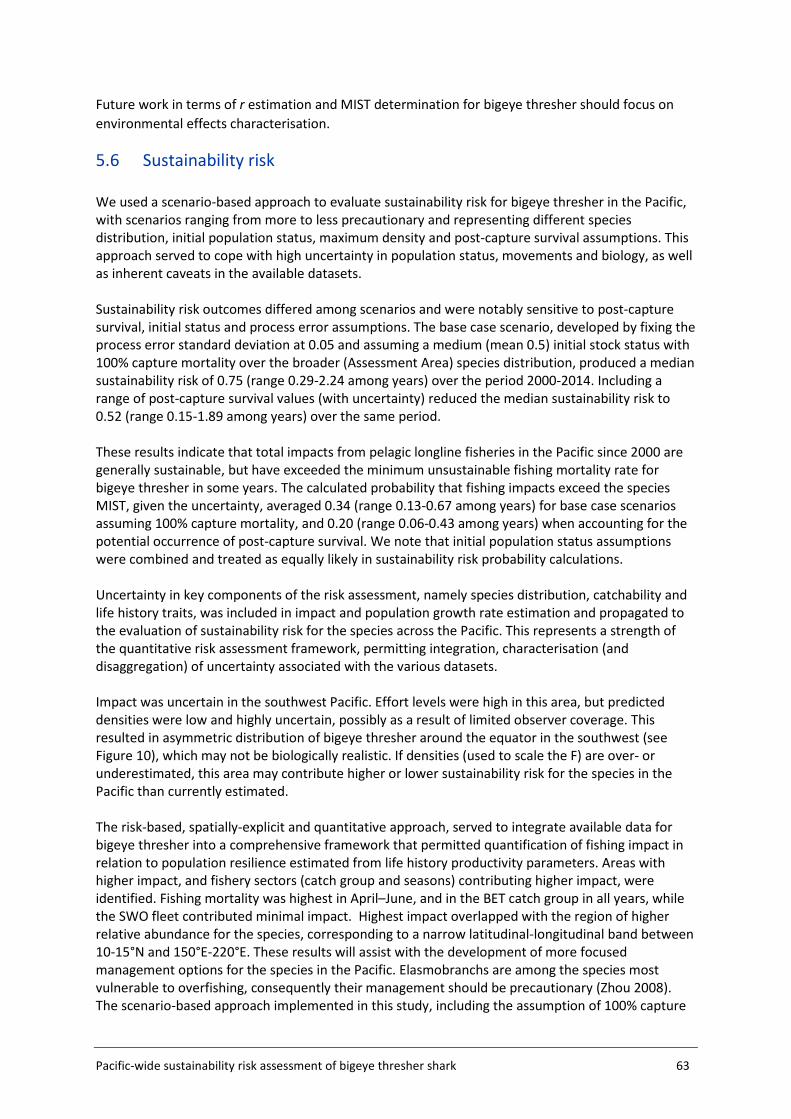
Pacific-wide sustainability risk assessment of bigeye thresher shark 63
Future work in terms of r estimation and MIST determination for bigeye thresher should focus on environmental effects characterisation.
5.6 Sustainability risk We used a scenario-based approach to evaluate sustainability risk for bigeye thresher in the Pacific, with scenarios ranging from more to less precautionary and representing different species distribution, initial population status, maximum density and post-capture survival assumptions. This approach served to cope with high uncertainty in population status, movements and biology, as well as inherent caveats in the available datasets. Sustainability risk outcomes differed among scenarios and were notably sensitive to post-capture survival, initial status and process error assumptions. The base case scenario, developed by fixing the process error standard deviation at 0.05 and assuming a medium (mean 0.5) initial stock status with 100% capture mortality over the broader (Assessment Area) species distribution, produced a median sustainability risk of 0.75 (range 0.29-2.24 among years) over the period 2000-2014. Including a range of post-capture survival values (with uncertainty) reduced the median sustainability risk to 0.52 (range 0.15-1.89 among years) over the same period. These results indicate that total impacts from pelagic longline fisheries in the Pacific since 2000 are generally sustainable, but have exceeded the minimum unsustainable fishing mortality rate for bigeye thresher in some years. The calculated probability that fishing impacts exceed the species MIST, given the uncertainty, averaged 0.34 (range 0.13-0.67 among years) for base case scenarios assuming 100% capture mortality, and 0.20 (range 0.06-0.43 among years) when accounting for the potential occurrence of post-capture survival. We note that initial population status assumptions were combined and treated as equally likely in sustainability risk probability calculations. Uncertainty in key components of the risk assessment, namely species distribution, catchability and life history traits, was included in impact and population growth rate estimation and propagated to the evaluation of sustainability risk for the species across the Pacific. This represents a strength of the quantitative risk assessment framework, permitting integration, characterisation (and disaggregation) of uncertainty associated with the various datasets. Impact was uncertain in the southwest Pacific. Effort levels were high in this area, but predicted densities were low and highly uncertain, possibly as a result of limited observer coverage. This resulted in asymmetric distribution of bigeye thresher around the equator in the southwest (see Figure 10), which may not be biologically realistic. If densities (used to scale the F) are over- or underestimated, this area may contribute higher or lower sustainability risk for the species in the Pacific than currently estimated. The risk-based, spatially-explicit and quantitative approach, served to integrate available data for bigeye thresher into a comprehensive framework that permitted quantification of fishing impact in relation to population resilience estimated from life history productivity parameters. Areas with higher impact, and fishery sectors (catch group and seasons) contributing higher impact, were identified. Fishing mortality was highest in April–June, and in the BET catch group in all years, while the SWO fleet contributed minimal impact. Highest impact overlapped with the region of higher relative abundance for the species, corresponding to a narrow latitudinal-longitudinal band between 10-15°N and 150°E-220°E. These results will assist with the development of more focused management options for the species in the Pacific. Elasmobranchs are among the species most vulnerable to overfishing, consequently their management should be precautionary (Zhou 2008). The scenario-based approach implemented in this study, including the assumption of 100% capture
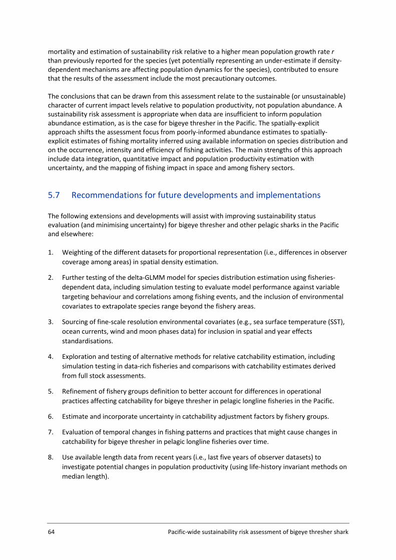
64 Pacific-wide sustainability risk assessment of bigeye thresher shark
mortality and estimation of sustainability risk relative to a higher mean population growth rate r than previously reported for the species (yet potentially representing an under-estimate if density-dependent mechanisms are affecting population dynamics for the species), contributed to ensure that the results of the assessment include the most precautionary outcomes. The conclusions that can be drawn from this assessment relate to the sustainable (or unsustainable) character of current impact levels relative to population productivity, not population abundance. A sustainability risk assessment is appropriate when data are insufficient to inform population abundance estimation, as is the case for bigeye thresher in the Pacific. The spatially-explicit approach shifts the assessment focus from poorly-informed abundance estimates to spatially-explicit estimates of fishing mortality inferred using available information on species distribution and on the occurrence, intensity and efficiency of fishing activities. The main strengths of this approach include data integration, quantitative impact and population productivity estimation with uncertainty, and the mapping of fishing impact in space and among fishery sectors.
5.7 Recommendations for future developments and implementations The following extensions and developments will assist with improving sustainability status evaluation (and minimising uncertainty) for bigeye thresher and other pelagic sharks in the Pacific and elsewhere: 1. Weighting of the different datasets for proportional representation (i.e., differences in observer
coverage among areas) in spatial density estimation.
2. Further testing of the delta-GLMM model for species distribution estimation using fisheries-dependent data, including simulation testing to evaluate model performance against variable targeting behaviour and correlations among fishing events, and the inclusion of environmental covariates to extrapolate species range beyond the fishery areas.
3. Sourcing of fine-scale resolution environmental covariates (e.g., sea surface temperature (SST), ocean currents, wind and moon phases data) for inclusion in spatial and year effects standardisations.
4. Exploration and testing of alternative methods for relative catchability estimation, including simulation testing in data-rich fisheries and comparisons with catchability estimates derived from full stock assessments.
5. Refinement of fishery groups definition to better account for differences in operational practices affecting catchability for bigeye thresher in pelagic longline fisheries in the Pacific.
6. Estimate and incorporate uncertainty in catchability adjustment factors by fishery groups.
7. Evaluation of temporal changes in fishing patterns and practices that might cause changes in catchability for bigeye thresher in pelagic longline fisheries over time.
8. Use available length data from recent years (i.e., last five years of observer datasets) to investigate potential changes in population productivity (using life-history invariant methods on median length).
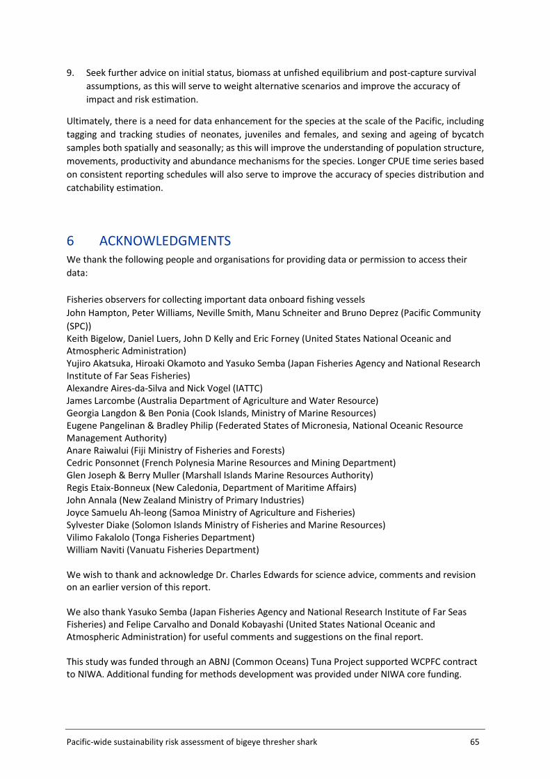
Pacific-wide sustainability risk assessment of bigeye thresher shark 65
9. Seek further advice on initial status, biomass at unfished equilibrium and post-capture survival assumptions, as this will serve to weight alternative scenarios and improve the accuracy of impact and risk estimation.
Ultimately, there is a need for data enhancement for the species at the scale of the Pacific, including tagging and tracking studies of neonates, juveniles and females, and sexing and ageing of bycatch samples both spatially and seasonally; as this will improve the understanding of population structure, movements, productivity and abundance mechanisms for the species. Longer CPUE time series based on consistent reporting schedules will also serve to improve the accuracy of species distribution and catchability estimation.
6 ACKNOWLEDGMENTS We thank the following people and organisations for providing data or permission to access their data: Fisheries observers for collecting important data onboard fishing vessels John Hampton, Peter Williams, Neville Smith, Manu Schneiter and Bruno Deprez (Pacific Community (SPC)) Keith Bigelow, Daniel Luers, John D Kelly and Eric Forney (United States National Oceanic and Atmospheric Administration) Yujiro Akatsuka, Hiroaki Okamoto and Yasuko Semba (Japan Fisheries Agency and National Research Institute of Far Seas Fisheries) Alexandre Aires-da-Silva and Nick Vogel (IATTC) James Larcombe (Australia Department of Agriculture and Water Resource) Georgia Langdon & Ben Ponia (Cook Islands, Ministry of Marine Resources) Eugene Pangelinan & Bradley Philip (Federated States of Micronesia, National Oceanic Resource Management Authority) Anare Raiwalui (Fiji Ministry of Fisheries and Forests) Cedric Ponsonnet (French Polynesia Marine Resources and Mining Department) Glen Joseph & Berry Muller (Marshall Islands Marine Resources Authority) Regis Etaix-Bonneux (New Caledonia, Department of Maritime Affairs) John Annala (New Zealand Ministry of Primary Industries) Joyce Samuelu Ah-leong (Samoa Ministry of Agriculture and Fisheries) Sylvester Diake (Solomon Islands Ministry of Fisheries and Marine Resources) Vilimo Fakalolo (Tonga Fisheries Department) William Naviti (Vanuatu Fisheries Department) We wish to thank and acknowledge Dr. Charles Edwards for science advice, comments and revision on an earlier version of this report. We also thank Yasuko Semba (Japan Fisheries Agency and National Research Institute of Far Seas Fisheries) and Felipe Carvalho and Donald Kobayashi (United States National Oceanic and Atmospheric Administration) for useful comments and suggestions on the final report. This study was funded through an ABNJ (Common Oceans) Tuna Project supported WCPFC contract to NIWA. Additional funding for methods development was provided under NIWA core funding.
66 Pacific-wide sustainability risk assessment of bigeye thresher shark
7 REFERENCES Amorim, A. et al. 2009. Alopias superciliosus. The IUCN Red List of Threatened Species 2009: e.T161696A5482468. http://dx.doi.org/10.2305/IUCN.UK.2009-2.RLTS.T161696A5482468.en Bentley, N., Kendrick, T. H., Starr, P. J., Breen, P. A. (2011) Influence plots and metrics: tools for better understanding fisheries catch-per-unit-effort standardisations. ICES Journal of Marine Science, 69: 84-88. Braccini, J. M., Gillanders, B. M., & Walker, T. I. 2006. Hierarchical approach to the assessment of fishing effects on non-target chondrichthyans: case study of Squalus megalops in southeastern Australia. Canadian Journal of Fisheries and Aquatic Sciences, 63, 2456-2466. Carvalho, J.F.D. (2014). Population dynamics and fisheries assessment of the bigeye thresher (Alopias superciliosus) in the Atlantic: a comparison between North Atlantic and South Atlantic stocks. PhD Thesis. Chen, C.-T., Liu, K.-M., Chang, Y.-C. 1997. Reproductive biology of the bigeye thresher shark, Alopias superciliosus (Lowe, 1839) (Chondrichthyes: Alopiidae), in the northwestern Pacific. Ichthyological Research 44, 227-235. Chen, P., Yuan, W. 2006. Demographic analysis based on the growth parameter of sharks. Fisheries Research 78, 374-379.
Clarke, S. 2009. An alternative estimate of catches of five species of sharks in the Western and Central Pacific Ocean based on shark fin trade data. Western and Central Pacific Fisheries Commission, Scientific Committee Paper SC5/EB-WP-02. Clarke, S. 2011. A status snapshot of key shark species in the Western and Central Pacific and potential management options. WCPFC-SC7-2011/EB-WP-04. Clarke, S., S. Harley, S. Hoyle and J. Rice. 2011a. An indicator-based analysis of key shark species based on data held by SPC-OFP. WCPFC-SC7-2011/EB-WP-01. Accessed online at https://www.wcpfc.int/node/2766 Clarke, S., Yokawa, K., Matsunaga, H. and Nakano, H. 2011b. Analysis of North Pacific shark data from Japanese commercial longline and research/training vessel records. WCPFC-SC7-2011/EB-WP-02. Clarke S., M. Sato, C. Small, B. Sullivan, Y. Inoue and D. Ochi. 2014a. Bycatch in longline fisheries for tuna and tuna-like species: A global review of status and mitigation measures. FAO Fisheries Technical Paper 588. Rome. 199 p. Clarke, S., L. Manarangi-Trott and S. Brouwer. 2014b. Issues for t-RFMOs in relation to the listing of shark and ray species by the Convention on International Trade in Endangered Species (CITES). WCPFC-SC10-2014/EP-IP-05. Accessed online at http://www.wcpfc.int/system/files/EB-IP-05%20(CITES%20%20Sharks).pdf Clarke, S., R. Coelho, M. Francis, M. Kai, S. Kohin, K.M. Liu, C. Simpfendorfer, J. Tovar-Avila, C. Rigby and J. Smart. 2015. Report of the Pacific Shark Life History Expert Panel Workshop, 28-30 April 2015. WCPFC-SC11-2015/EB-IP-13.
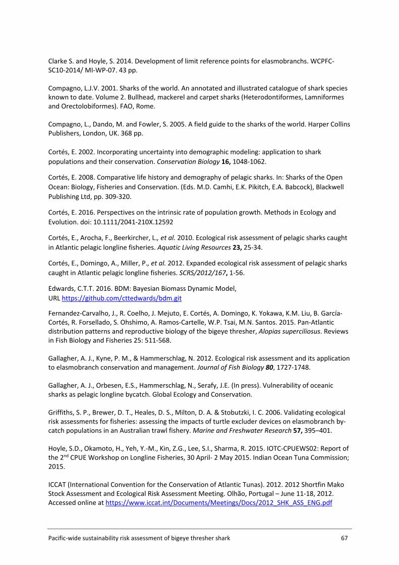
Pacific-wide sustainability risk assessment of bigeye thresher shark 67
Clarke S. and Hoyle, S. 2014. Development of limit reference points for elasmobranchs. WCPFC-SC10-2014/ MI-WP-07. 43 pp. Compagno, L.J.V. 2001. Sharks of the world. An annotated and illustrated catalogue of shark species known to date. Volume 2. Bullhead, mackerel and carpet sharks (Heterodontiformes, Lamniformes and Orectolobiformes). FAO, Rome. Compagno, L., Dando, M. and Fowler, S. 2005. A field guide to the sharks of the world. Harper Collins Publishers, London, UK. 368 pp. Cortés, E. 2002. Incorporating uncertainty into demographic modeling: application to shark populations and their conservation. Conservation Biology 16, 1048-1062.
Cortés, E. 2008. Comparative life history and demography of pelagic sharks. In: Sharks of the Open Ocean: Biology, Fisheries and Conservation. (Eds. M.D. Camhi, E.K. Pikitch, E.A. Babcock), Blackwell Publishing Ltd, pp. 309-320.
Cortés, E. 2016. Perspectives on the intrinsic rate of population growth. Methods in Ecology and Evolution. doi: 10.1111/2041-210X.12592
Cortés, E., Arocha, F., Beerkircher, L., et al. 2010. Ecological risk assessment of pelagic sharks caught in Atlantic pelagic longline fisheries. Aquatic Living Resources 23, 25-34.
Cortés, E., Domingo, A., Miller, P., et al. 2012. Expanded ecological risk assessment of pelagic sharks caught in Atlantic pelagic longline fisheries. SCRS/2012/167, 1-56.
Edwards, C.T.T. 2016. BDM: Bayesian Biomass Dynamic Model, URL https://github.com/cttedwards/bdm.git
Fernandez-Carvalho, J., R. Coelho, J. Mejuto, E. Cortés, A. Domingo, K. Yokawa, K.M. Liu, B. García-Cortés, R. Forsellado, S. Ohshimo, A. Ramos-Cartelle, W.P. Tsai, M.N. Santos. 2015. Pan-Atlantic distribution patterns and reproductive biology of the bigeye thresher, Alopias superciliosus. Reviews in Fish Biology and Fisheries 25: 511-568. Gallagher, A. J., Kyne, P. M., & Hammerschlag, N. 2012. Ecological risk assessment and its application to elasmobranch conservation and management. Journal of Fish Biology 80, 1727-1748. Gallagher, A. J., Orbesen, E.S., Hammerschlag, N., Serafy, J.E. (In press). Vulnerability of oceanic sharks as pelagic longline bycatch. Global Ecology and Conservation. Griffiths, S. P., Brewer, D. T., Heales, D. S., Milton, D. A. & Stobutzki, I. C. 2006. Validating ecological risk assessments for fisheries: assessing the impacts of turtle excluder devices on elasmobranch by-catch populations in an Australian trawl fishery. Marine and Freshwater Research 57, 395–401. Hoyle, S.D., Okamoto, H., Yeh, Y.-M., Kin, Z.G., Lee, S.I., Sharma, R. 2015. IOTC-CPUEWS02: Report of the 2nd CPUE Workshop on Longline Fisheries, 30 April- 2 May 2015. Indian Ocean Tuna Commission; 2015. ICCAT (International Convention for the Conservation of Atlantic Tunas). 2012. 2012 Shortfin Mako Stock Assessment and Ecological Risk Assessment Meeting. Olhão, Portugal – June 11-18, 2012. Accessed online at https://www.iccat.int/Documents/Meetings/Docs/2012_SHK_ASS_ENG.pdf
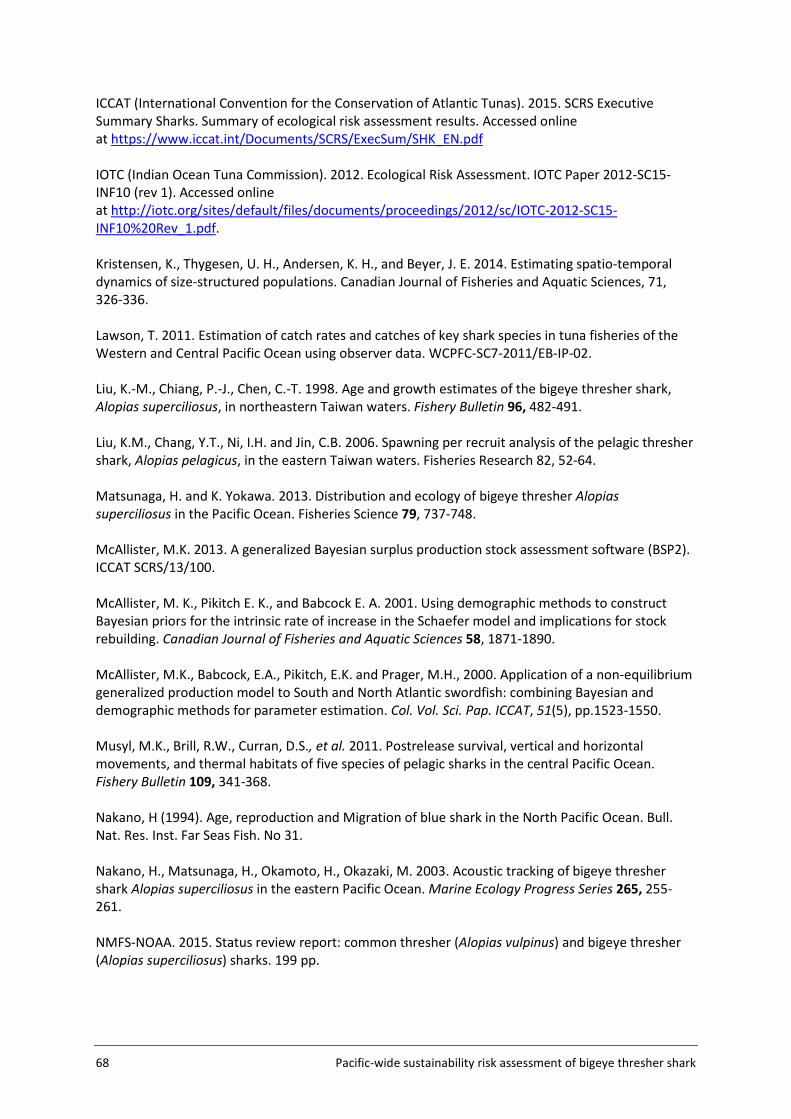
68 Pacific-wide sustainability risk assessment of bigeye thresher shark
ICCAT (International Convention for the Conservation of Atlantic Tunas). 2015. SCRS Executive Summary Sharks. Summary of ecological risk assessment results. Accessed online at https://www.iccat.int/Documents/SCRS/ExecSum/SHK_EN.pdf IOTC (Indian Ocean Tuna Commission). 2012. Ecological Risk Assessment. IOTC Paper 2012-SC15-INF10 (rev 1). Accessed online at http://iotc.org/sites/default/files/documents/proceedings/2012/sc/IOTC-2012-SC15-INF10%20Rev_1.pdf. Kristensen, K., Thygesen, U. H., Andersen, K. H., and Beyer, J. E. 2014. Estimating spatio-temporal dynamics of size-structured populations. Canadian Journal of Fisheries and Aquatic Sciences, 71, 326-336. Lawson, T. 2011. Estimation of catch rates and catches of key shark species in tuna fisheries of the Western and Central Pacific Ocean using observer data. WCPFC-SC7-2011/EB-IP-02. Liu, K.-M., Chiang, P.-J., Chen, C.-T. 1998. Age and growth estimates of the bigeye thresher shark, Alopias superciliosus, in northeastern Taiwan waters. Fishery Bulletin 96, 482-491. Liu, K.M., Chang, Y.T., Ni, I.H. and Jin, C.B. 2006. Spawning per recruit analysis of the pelagic thresher shark, Alopias pelagicus, in the eastern Taiwan waters. Fisheries Research 82, 52-64. Matsunaga, H. and K. Yokawa. 2013. Distribution and ecology of bigeye thresher Alopias superciliosus in the Pacific Ocean. Fisheries Science 79, 737-748. McAllister, M.K. 2013. A generalized Bayesian surplus production stock assessment software (BSP2). ICCAT SCRS/13/100. McAllister, M. K., Pikitch E. K., and Babcock E. A. 2001. Using demographic methods to construct Bayesian priors for the intrinsic rate of increase in the Schaefer model and implications for stock rebuilding. Canadian Journal of Fisheries and Aquatic Sciences 58, 1871-1890. McAllister, M.K., Babcock, E.A., Pikitch, E.K. and Prager, M.H., 2000. Application of a non-equilibrium generalized production model to South and North Atlantic swordfish: combining Bayesian and demographic methods for parameter estimation. Col. Vol. Sci. Pap. ICCAT, 51(5), pp.1523-1550. Musyl, M.K., Brill, R.W., Curran, D.S., et al. 2011. Postrelease survival, vertical and horizontal movements, and thermal habitats of five species of pelagic sharks in the central Pacific Ocean. Fishery Bulletin 109, 341-368. Nakano, H (1994). Age, reproduction and Migration of blue shark in the North Pacific Ocean. Bull. Nat. Res. Inst. Far Seas Fish. No 31. Nakano, H., Matsunaga, H., Okamoto, H., Okazaki, M. 2003. Acoustic tracking of bigeye thresher shark Alopias superciliosus in the eastern Pacific Ocean. Marine Ecology Progress Series 265, 255-261. NMFS-NOAA. 2015. Status review report: common thresher (Alopias vulpinus) and bigeye thresher (Alopias superciliosus) sharks. 199 pp.
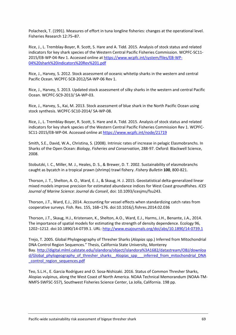
Pacific-wide sustainability risk assessment of bigeye thresher shark 69
Polacheck, T. (1991). Measures of effort in tuna longline fisheries: changes at the operational level. Fisheries Research 12:75–87. Rice, J., L. Tremblay-Boyer, R. Scott, S. Hare and A. Tidd. 2015. Analysis of stock status and related indicators for key shark species of the Western Central Pacific Fisheries Commission. WCPFC-SC11-2015/EB-WP-04-Rev 1. Accessed online at https://www.wcpfc.int/system/files/EB-WP-04%20shark%20indicators%20Rev%201.pdf Rice, J., Harvey, S. 2012. Stock assessment of oceanic whitetip sharks in the western and central Pacific Ocean. WCPFC-SC8-2012/SA-WP-06 Rev 1. Rice, J., Harvey, S. 2013. Updated stock assessment of silky sharks in the western and central Pacific Ocean. WCPFC-SC9-2013/ SA-WP-03. Rice, J., Harvey, S., Kai, M. 2013. Stock assessment of blue shark in the North Pacific Ocean using stock synthesis. WCPFC-SC10-2014/ SA-WP-08. Rice, J., L. Tremblay-Boyer, R. Scott, S. Hare and A. Tidd. 2015. Analysis of stock status and related indicators for key shark species of the Western Central Pacific Fisheries Commission Rev 1. WCPFC-SC11-2015/EB-WP-04. Accessed online at https://www.wcpfc.int/node/21719 Smith, S.E., David, W.A., Christina, S. (2008). Intrinsic rates of increase in pelagic Elasmobranchs. In Sharks of the Open Ocean: Biology, Fisheries and Conservation, 288-97. Oxford: Blackwell Science, 2008. Stobutzki, I. C., Miller, M. J., Heales, D. S., & Brewer, D. T. 2002. Sustainability of elasmobranchs caught as bycatch in a tropical prawn (shrimp) trawl fishery. Fishery Bulletin 100, 800-821. Thorson, J. T., Shelton, A. O., Ward, E. J., & Skaug, H. J. 2015. Geostatistical delta-generalized linear mixed models improve precision for estimated abundance indices for West Coast groundfishes. ICES Journal of Marine Science: Journal du Conseil, doi: 10.1093/icesjms/fsu243. Thorson, J.T., Ward, E.J., 2014. Accounting for vessel effects when standardizing catch rates from cooperative surveys. Fish. Res. 155, 168–176. doi:10.1016/j.fishres.2014.02.036 Thorson, J.T., Skaug, H.J., Kristensen, K., Shelton, A.O., Ward, E.J., Harms, J.H., Benante, J.A., 2014. The importance of spatial models for estimating the strength of density dependence. Ecology 96, 1202–1212. doi:10.1890/14-0739.1. URL: http://www.esajournals.org/doi/abs/10.1890/14-0739.1 Trejo, T. 2005. Global Phylogeography of Thresher Sharks (Alopias spp.) Inferred from Mitochondrial DNA Control Region Sequences.” Thesis, California State University, Monterey Bay. http://digital.mlml.calstate.edu/islandora/object/islandora%3A1682/datastream/OBJ/download/Global_phylogeography_of_thresher_sharks__Alopias_spp___inferred_from_mitochondrial_DNA_control_region_sequences.pdf Teo, S.L.H., E. Garcia Rodriguez and O. Sosa-Nishizaki. 2016. Status of Common Thresher Sharks, Alopias vulpinus, along the West Coast of North America. NOAA Technical Memorandum (NOAA-TM-NMFS-SWFSC-557), Southwest Fisheries Science Center, La Jolla, California. 198 pp.
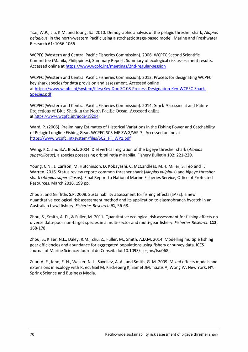
70 Pacific-wide sustainability risk assessment of bigeye thresher shark
Tsai, W.P., Liu, K.M. and Joung, S.J. 2010. Demographic analysis of the pelagic thresher shark, Alopias pelagicus, in the north-western Pacific using a stochastic stage-based model. Marine and Freshwater Research 61: 1056-1066. WCPFC (Western and Central Pacific Fisheries Commission). 2006. WCPFC Second Scientific Committee (Manila, Philippines), Summary Report. Summary of ecological risk assessment results. Accessed online at https://www.wcpfc.int/meetings/2nd-regular-session WCPFC (Western and Central Pacific Fisheries Commission). 2012. Process for designating WCPFC key shark species for data provision and assessment. Accessed online at https://www.wcpfc.int/system/files/Key-Doc-SC-08-Process-Designation-Key-WCPFC-Shark-Species.pdf WCPFC (Western and Central Pacific Fisheries Commission). 2014. Stock Assessment and Future Projections of Blue Shark in the North Pacific Ocean. Accessed online at https://www.wcpfc.int/node/19204 Ward, P. (2006). Preliminary Estimates of Historical Variations in the Fishing Power and Catchability of Pelagic Longline Fishing Gear. WCPFC-SC3-ME SWG/WP-7. Accessed online at https://www.wcpfc.int/system/files/SC2_FT_WP1.pdf Weng, K.C. and B.A. Block. 2004. Diel vertical migration of the bigeye thresher shark (Alopias superciliosus), a species possessing orbital retia mirabilia. Fishery Bulletin 102: 221-229. Young, C.N., J. Carlson, M. Hutchinson, D. Kobayashi, C. McCandless, M.H. Miller, S. Teo and T. Warren. 2016. Status review report: common thresher shark (Alopias vulpinus) and bigeye thresher shark (Alopias superciliosus). Final Report to National Marine Fisheries Service, Office of Protected Resources. March 2016. 199 pp. Zhou S. and Griffiths S.P. 2008. Sustainability assessment for fishing effects (SAFE): a new quantitative ecological risk assessment method and its application to elasmobranch bycatch in an Australian trawl fishery. Fisheries Research 91, 56-68. Zhou, S., Smith, A. D., & Fuller, M. 2011. Quantitative ecological risk assessment for fishing effects on diverse data-poor non-target species in a multi-sector and multi-gear fishery. Fisheries Research 112, 168-178. Zhou, S., Klaer, N.L., Daley, R.M., Zhu, Z., Fuller, M., Smith, A.D.M. 2014. Modelling multiple fishing gear efficiencies and abundance for aggregated populations using fishery or survey data. ICES Journal of Marine Science: Journal du Conseil. doi:10.1093/icesjms/fsu068. Zuur, A. F., Ieno, E. N., Walker, N. J., Saveliev, A. A., and Smith, G. M. 2009. Mixed effects models and extensions in ecology with R; ed. Gail M, Krickeberg K, Samet JM, Tsiatis A, Wong W. New York, NY: Spring Science and Business Media.
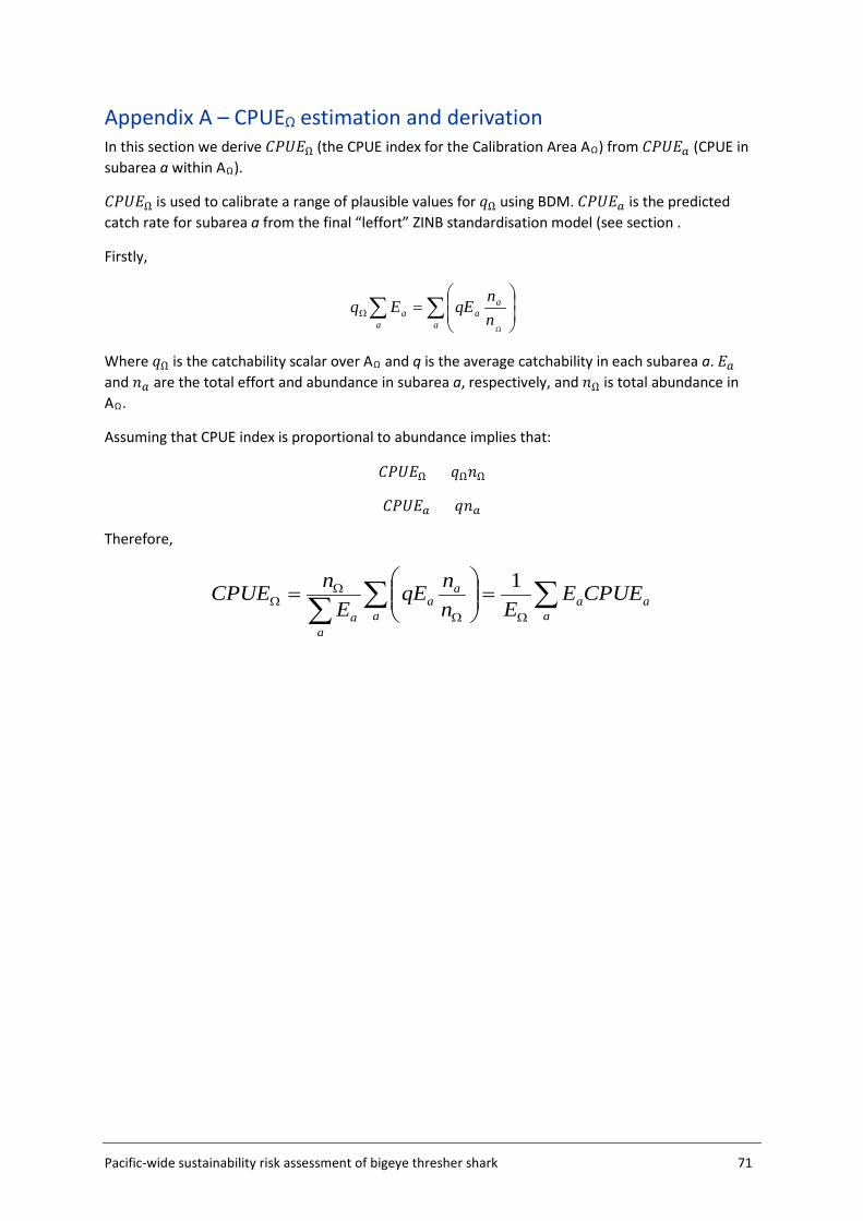
Pacific-wide sustainability risk assessment of bigeye thresher shark 71
Appendix A – CPUEΩ estimation and derivation In this section we derive 𝐶𝐶𝐶𝐶𝐶𝐶𝐶𝐶Ω (the CPUE index for the Calibration Area AΩ) from 𝐶𝐶𝐶𝐶𝐶𝐶𝐶𝐶𝑠𝑠 (CPUE in subarea a within AΩ).
𝐶𝐶𝐶𝐶𝐶𝐶𝐶𝐶Ω is used to calibrate a range of plausible values for 𝑞𝑞Ω using BDM. 𝐶𝐶𝐶𝐶𝐶𝐶𝐶𝐶𝑠𝑠 is the predicted catch rate for subarea a from the final “leffort” ZINB standardisation model (see section .
Firstly,
∑∑
=
Ω
Ωa
aa
aa n
nqEEq
Where 𝑞𝑞Ω is the catchability scalar over AΩ and q is the average catchability in each subarea a. 𝐶𝐶𝑠𝑠 and 𝑛𝑛𝑠𝑠 are the total effort and abundance in subarea a, respectively, and 𝑛𝑛Ω is total abundance in AΩ.
Assuming that CPUE index is proportional to abundance implies that:
𝐶𝐶𝐶𝐶𝐶𝐶𝐶𝐶Ω = 𝑞𝑞Ω𝑛𝑛Ω
𝐶𝐶𝐶𝐶𝐶𝐶𝐶𝐶𝑠𝑠 = 𝑞𝑞𝑛𝑛𝑠𝑠
Therefore,
∑∑∑ ΩΩ
ΩΩ =
=
aaa
a
aa
aa
CPUEEEn
nqEE
nCPUE 1
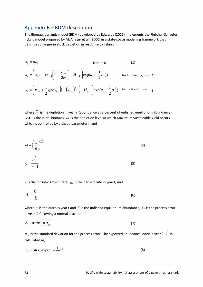
72 Pacific-wide sustainability risk assessment of bigeye thresher shark
Appendix B – BDM description The Biomass dynamic model (BDM) developed by Edwards (2016) implements the Fletcher-Schaefer hybrid model proposed by McAllister et al. (2000) in a state-space modelling framework that describes changes in stock depletion in response to fishing,:
00 µε=x 0for =t (1)
)21exp(
21 2
11
11 pttx
ttt Hx
rxxx σεϕ
−
−
−+= −
−−− ϕ<> txt and 0for (2)
( )( ) )21exp(1
21 2
11
111 pttn
tttt Hxxgrxx σεϕ −
−−+= −
−
−−− ϕ≥> txt and 0for (3)
where tx is the depletion in year t (abundance as a percent of unfished equilibrium abundance); u is the initial biomass; ϕ is the depletion level at which Maximum Sustainable Yield occurs,
which is controlled by a shape parametern , and
11
1 −
=
n
nϕ (4)
1
1
−=
−
nng
nn
(5)
r is the intrinsic growth rate. tH is the harvest rate in year t, and
KC
H tt = (6)
where tC is the catch is year t and K is the unfished equilibrium abundance, tε is the process error in year t following a normal distribution:
( )2,0 normal~ pt σε (7)
pσ is the standard deviation for the process error. The expected abundance index in year t , tI is
calculated as,
)21exp(ˆ 2
ottt qKxI σξ −= (8)
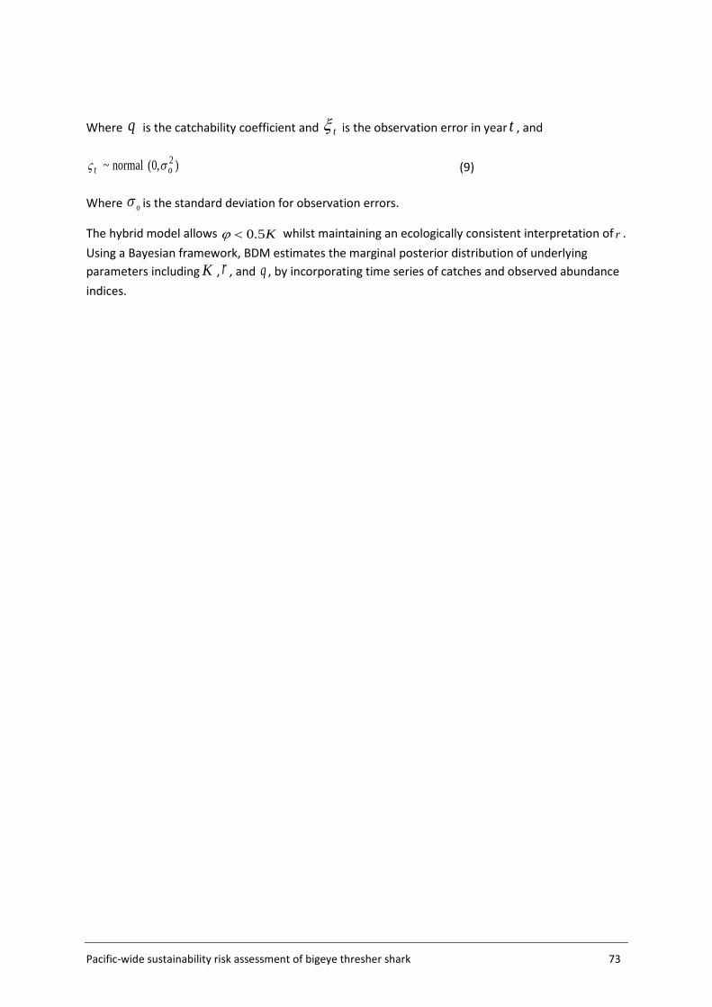
Pacific-wide sustainability risk assessment of bigeye thresher shark 73
Where q is the catchability coefficient and tξ is the observation error in year t , and
),0( normal~ 2ot σς (9)
Where oσ is the standard deviation for observation errors.
The hybrid model allows K5.0<ϕ whilst maintaining an ecologically consistent interpretation of r . Using a Bayesian framework, BDM estimates the marginal posterior distribution of underlying parameters including K , r , and q , by incorporating time series of catches and observed abundance indices.
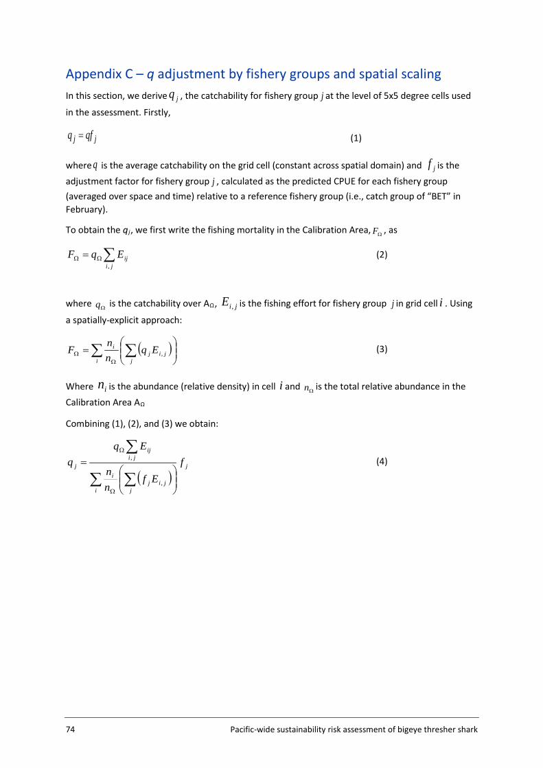
74 Pacific-wide sustainability risk assessment of bigeye thresher shark
Appendix C – q adjustment by fishery groups and spatial scaling In this section, we derive jq , the catchability for fishery group j at the level of 5x5 degree cells used
in the assessment. Firstly,
jj qfq = (1)
where q is the average catchability on the grid cell (constant across spatial domain) and jf is the adjustment factor for fishery group j , calculated as the predicted CPUE for each fishery group (averaged over space and time) relative to a reference fishery group (i.e., catch group of “BET” in February).
To obtain the qj, we first write the fishing mortality in the Calibration Area, ΩF , as
∑ΩΩ =ji
ijEqF,
(2)
where Ωq is the catchability over AΩ, jiE , is the fishing effort for fishery group j in grid cell i . Using
a spatially-explicit approach:
( )∑ ∑
=
ΩΩ
i jjij
i Eqnn
F , (3)
Where in is the abundance (relative density) in cell i and Ωn is the total relative abundance in the Calibration Area AΩ
Combining (1), (2), and (3) we obtain:
( )j
i jjij
i
jiij
j fEf
nn
Eqq
∑ ∑
∑
=
Ω
Ω
,
, (4)
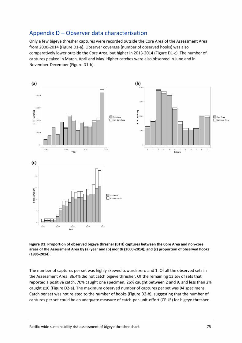
Pacific-wide sustainability risk assessment of bigeye thresher shark 75
Appendix D – Observer data characterisation Only a few bigeye thresher captures were recorded outside the Core Area of the Assessment Area from 2000-2014 (Figure D1-a). Observer coverage (number of observed hooks) was also comparatively lower outside the Core Area, but higher in 2013-2014 (Figure D1-c). The number of captures peaked in March, April and May. Higher catches were also observed in June and in November-December (Figure D1-b).
Figure D1: Proportion of observed bigeye thresher (BTH) captures between the Core Area and non-core areas of the Assessment Area by (a) year and (b) month (2000-2014); and (c) proportion of observed hooks (1995-2014).
The number of captures per set was highly skewed towards zero and 1. Of all the observed sets in the Assessment Area, 86.4% did not catch bigeye thresher. Of the remaining 13.6% of sets that reported a positive catch, 70% caught one specimen, 26% caught between 2 and 9, and less than 2% caught ≥10 (Figure D2-a). The maximum observed number of captures per set was 94 specimens. Catch per set was not related to the number of hooks (Figure D2-b), suggesting that the number of captures per set could be an adequate measure of catch-per-unit-effort (CPUE) for bigeye thresher.
(a)
(b)
(c)
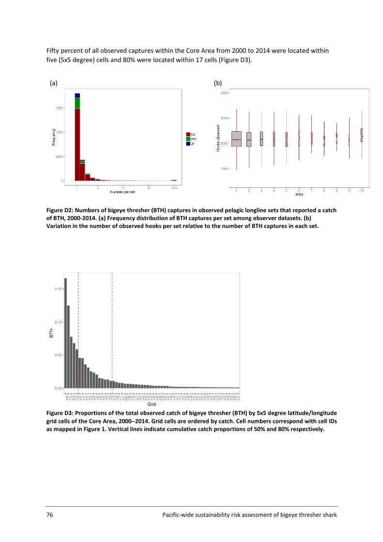
76 Pacific-wide sustainability risk assessment of bigeye thresher shark
Fifty percent of all observed captures within the Core Area from 2000 to 2014 were located within five (5x5 degree) cells and 80% were located within 17 cells (Figure D3).
Figure D2: Numbers of bigeye thresher (BTH) captures in observed pelagic longline sets that reported a catch of BTH, 2000-2014. (a) Frequency distribution of BTH captures per set among observer datasets. (b) Variation in the number of observed hooks per set relative to the number of BTH captures in each set.
Figure D3: Proportions of the total observed catch of bigeye thresher (BTH) by 5x5 degree latitude/longitude grid cells of the Core Area, 2000−2014. Grid cells are ordered by catch. Cell numbers correspond with cell IDs as mapped in Figure 1. Vertical lines indicate cumulative catch proportions of 50% and 80% respectively.
(a)
(b)
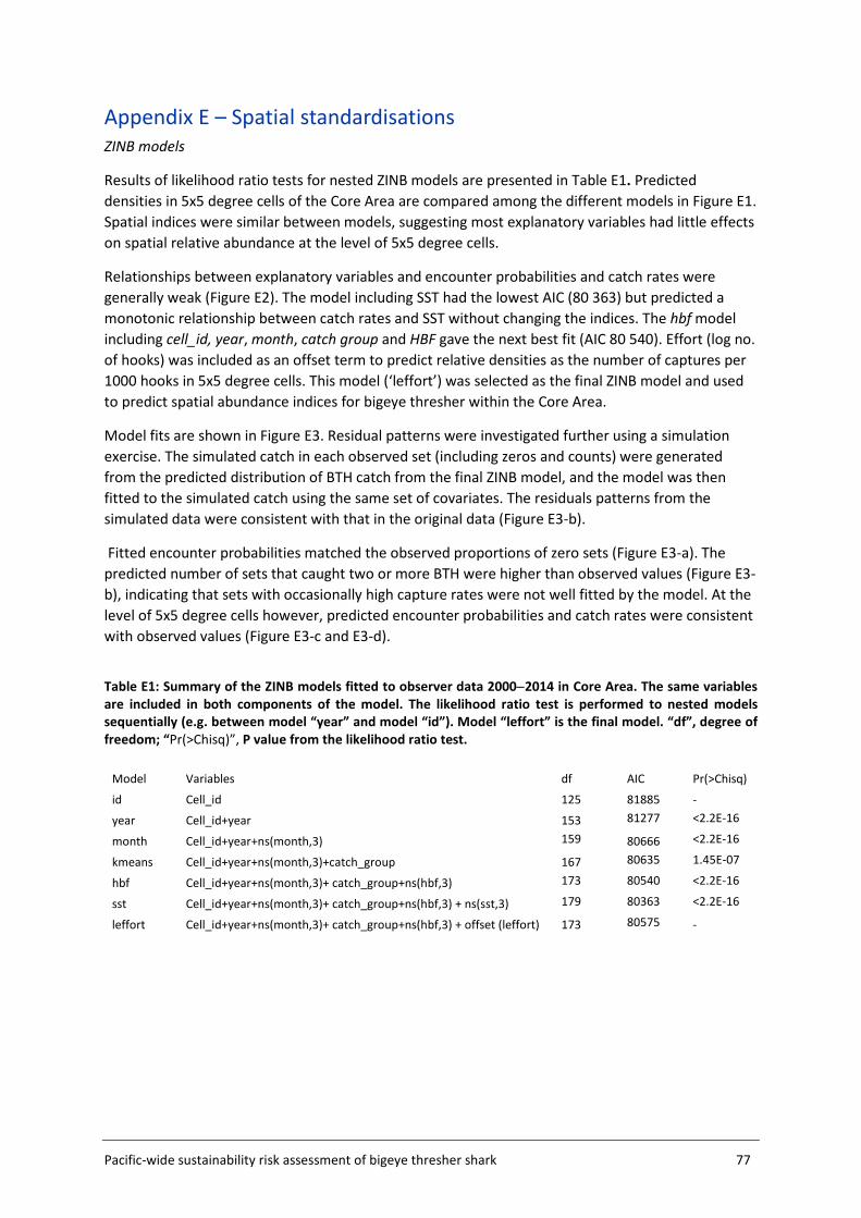
Pacific-wide sustainability risk assessment of bigeye thresher shark 77
Appendix E – Spatial standardisations ZINB models
Results of likelihood ratio tests for nested ZINB models are presented in Table E1. Predicted densities in 5x5 degree cells of the Core Area are compared among the different models in Figure E1. Spatial indices were similar between models, suggesting most explanatory variables had little effects on spatial relative abundance at the level of 5x5 degree cells.
Relationships between explanatory variables and encounter probabilities and catch rates were generally weak (Figure E2). The model including SST had the lowest AIC (80 363) but predicted a monotonic relationship between catch rates and SST without changing the indices. The hbf model including cell_id, year, month, catch group and HBF gave the next best fit (AIC 80 540). Effort (log no. of hooks) was included as an offset term to predict relative densities as the number of captures per 1000 hooks in 5x5 degree cells. This model (‘leffort’) was selected as the final ZINB model and used to predict spatial abundance indices for bigeye thresher within the Core Area.
Model fits are shown in Figure E3. Residual patterns were investigated further using a simulation exercise. The simulated catch in each observed set (including zeros and counts) were generated from the predicted distribution of BTH catch from the final ZINB model, and the model was then fitted to the simulated catch using the same set of covariates. The residuals patterns from the simulated data were consistent with that in the original data (Figure E3-b).
Fitted encounter probabilities matched the observed proportions of zero sets (Figure E3-a). The predicted number of sets that caught two or more BTH were higher than observed values (Figure E3-b), indicating that sets with occasionally high capture rates were not well fitted by the model. At the level of 5x5 degree cells however, predicted encounter probabilities and catch rates were consistent with observed values (Figure E3-c and E3-d).
Table E1: Summary of the ZINB models fitted to observer data 2000−2014 in Core Area. The same variables are included in both components of the model. The likelihood ratio test is performed to nested models sequentially (e.g. between model “year” and model “id”). Model “leffort” is the final model. “df”, degree of freedom; “Pr(>Chisq)”, P value from the likelihood ratio test.
Model Variables df AIC Pr(>Chisq)
id Cell_id 125 81885 -
year Cell_id+year 153 81277 <2.2E-16
month Cell_id+year+ns(month,3) 159 80666 <2.2E-16
kmeans Cell_id+year+ns(month,3)+catch_group 167 80635 1.45E-07
hbf Cell_id+year+ns(month,3)+ catch_group+ns(hbf,3) 173 80540 <2.2E-16
sst Cell_id+year+ns(month,3)+ catch_group+ns(hbf,3) + ns(sst,3) 179 80363 <2.2E-16
leffort Cell_id+year+ns(month,3)+ catch_group+ns(hbf,3) + offset (leffort) 173 80575 -
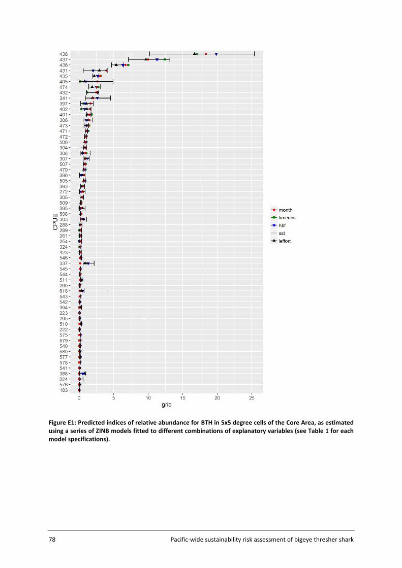
78 Pacific-wide sustainability risk assessment of bigeye thresher shark
Figure E1: Predicted indices of relative abundance for BTH in 5x5 degree cells of the Core Area, as estimated using a series of ZINB models fitted to different combinations of explanatory variables (see Table 1 for each model specifications).
Pacific-wide sustainability risk assessment of bigeye thresher shark 79
(a)
(b)
(c)
(d)
Figure E2: Relationships between encounter probabilities (in logit space) and BTH catch rates (in log space) in Core Area cells (2000−2014) as related to (a) catch group; (b) HBF (shallow sets (HBF <15) and deep sets (HBF ≥15)); (c) fishing duration at night (hours in darkness); and (d) wire trace (“U” represents unknown).
Residuals diagnostics for the final ZINB model are presented in Figure E4. Predicted catch rates by explanatory variables are shown in Figure E5. Highest catch rates occurred between March and May and again in November-December, and were associated with catch group ‘BET’.
80 Pacific-wide sustainability risk assessment of bigeye thresher shark
(a)
(b)
(c)
(d)
Figure E3: Predicted vs observed encounter probabilities and numbers of BTH per set for the final ZINB model “leffort” fitted to observer data in the Core Area, 2000−2014. (a) overall proportion of sets with zero catch (the bars on the left) and overall proportion of sets with positive catch); (b) distribution of catch per set; (c) encounter probabilities in each grid cell; (d) catch per set for in each grid cell.
Pacific-wide sustainability risk assessment of bigeye thresher shark 81
(a)
(b)
Figure E4: Residuals diagnostics for (a) the final ZINB (leffort) model fitted to Core Area observer data for the period 2000-2014; and (b) the same model fitted to simulated BTH catch data based on the predicted catch distribution derived from the final model. Pearson Residuals vs fitted values (top-left panel in both (a) and (b)); Observed catch vs fitted catch (top-right); Pearson Residuals by 5x5 degree cell (bottom-left); Pearson Residuals by year (bottom-right).
82 Pacific-wide sustainability risk assessment of bigeye thresher shark
Figure E5: Predicted CPUE (number of BTH per 1000 hooks) by covariate for the final ZINB model “leffort” fitted to observer data 2000−2014 in Core Area. Geostatistical delta-GLMM models
Estimated variance parameters for the three fitted delta-GLMM models are presented in Table E2. Spatial variability in encounter probabilities was greater than the spatial variability in positive catch rates. In the spatial model, density was correlated over a longer distance on the longitudinal axis (East-West plane) than on the North-South axis (Figure E6).
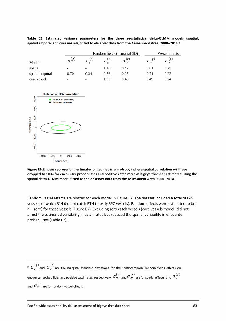
Pacific-wide sustainability risk assessment of bigeye thresher shark 83
Table E2: Estimated variance parameters for the three geostatistical delta-GLMM models (spatial, spatiotemporal and core vessels) fitted to observer data from the Assessment Area, 2000−2014. 5
Random fields (marginal SD) Vessel effects
Model )( p
εσ )(r
εσ )( p
ϖσ )(r
ϖσ )( p
vσ )(r
vσ
spatial - - 1.16 0.42 0.81 0.25 spatiotemporal 0.70 0.34 0.76 0.25 0.71 0.22 core vessels - - 1.05 0.43 0.49 0.24
Figure E6:Ellipses representing estimates of geometric anisotropy (where spatial correlation will have dropped to 10%) for encounter probabilities and positive catch rates of bigeye thresher estimated using the spatial delta-GLMM model fitted to the observer data from the Assessment Area, 2000−2014. Random vessel effects are plotted for each model in Figure E7. The dataset included a total of 849 vessels, of which 314 did not catch BTH (mostly SPC vessels). Random effects were estimated to be nil (zero) for these vessels (Figure E7). Excluding zero catch vessels (core vessels model) did not affect the estimated variability in catch rates but reduced the spatial variability in encounter probabilities (Table E2).
5
)( pεσ and
)(rεσ are the marginal standard deviations for the spatiotemporal random fields effects on
encounter probabilities and positive catch rates, respectively. )( p
ϖσ and)(r
ϖσ are for spatial effects; and )( p
vσ
and )(r
vσ are for random vessel effects.
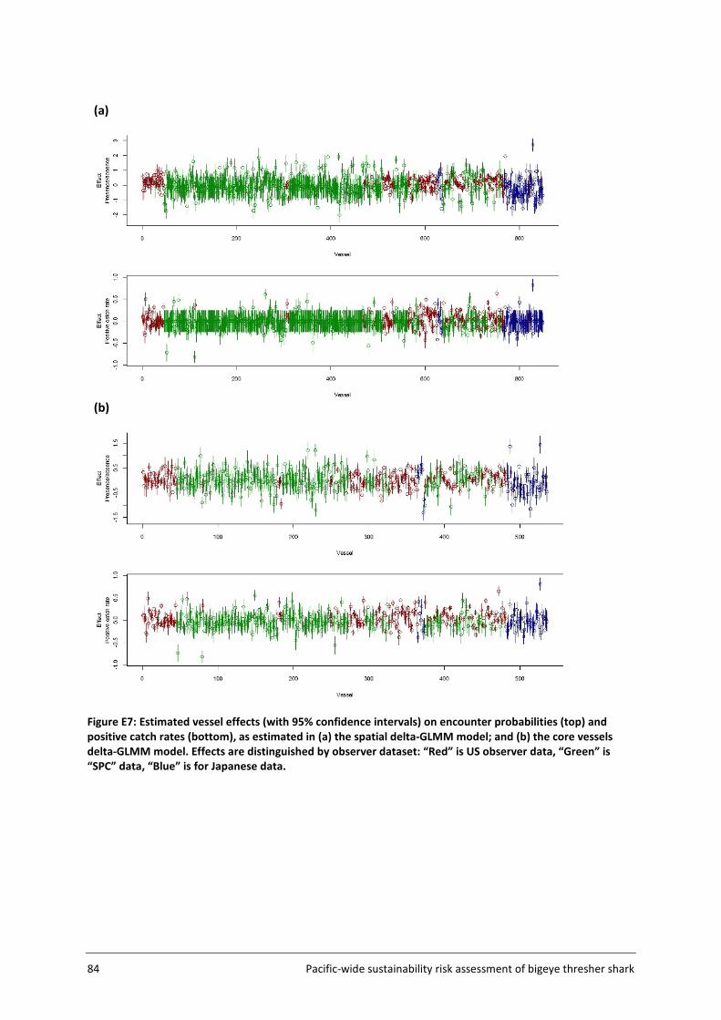
84 Pacific-wide sustainability risk assessment of bigeye thresher shark
Figure E7: Estimated vessel effects (with 95% confidence intervals) on encounter probabilities (top) and positive catch rates (bottom), as estimated in (a) the spatial delta-GLMM model; and (b) the core vessels delta-GLMM model. Effects are distinguished by observer dataset: “Red” is US observer data, “Green” is “SPC” data, “Blue” is for Japanese data.
(a)
(b)
Pacific-wide sustainability risk assessment of bigeye thresher shark 85
Appendix F – q calibration Results and sensitivities Time series of abundance and predicted abundance indices associated with the range of
Ωq values used in the assessment are shown in Figure F1. BDM-estimated depletion showed a similar trend among initial biomass level assumptions (Figure F1−a). Predicted abundance indices were consistent with the fitted index (Figure F1-b).
Posterior estimates for K with alternative prior bounds are shown in Figure F2. The use of bounds based on blue shark assessments (WCPFC 2016) resulted a much wider range of K being retained, but with decreasing probabilities for higher values (Figure F2-a). The mode of the posterior distributions was similar among the three assumed upper bound values. Posterior estimates for r were similar for these runs (Figure F2-b) and retained a range of values of r similar to the constructed prior (shown in Figure 23, section 4.4) (Figure F2).
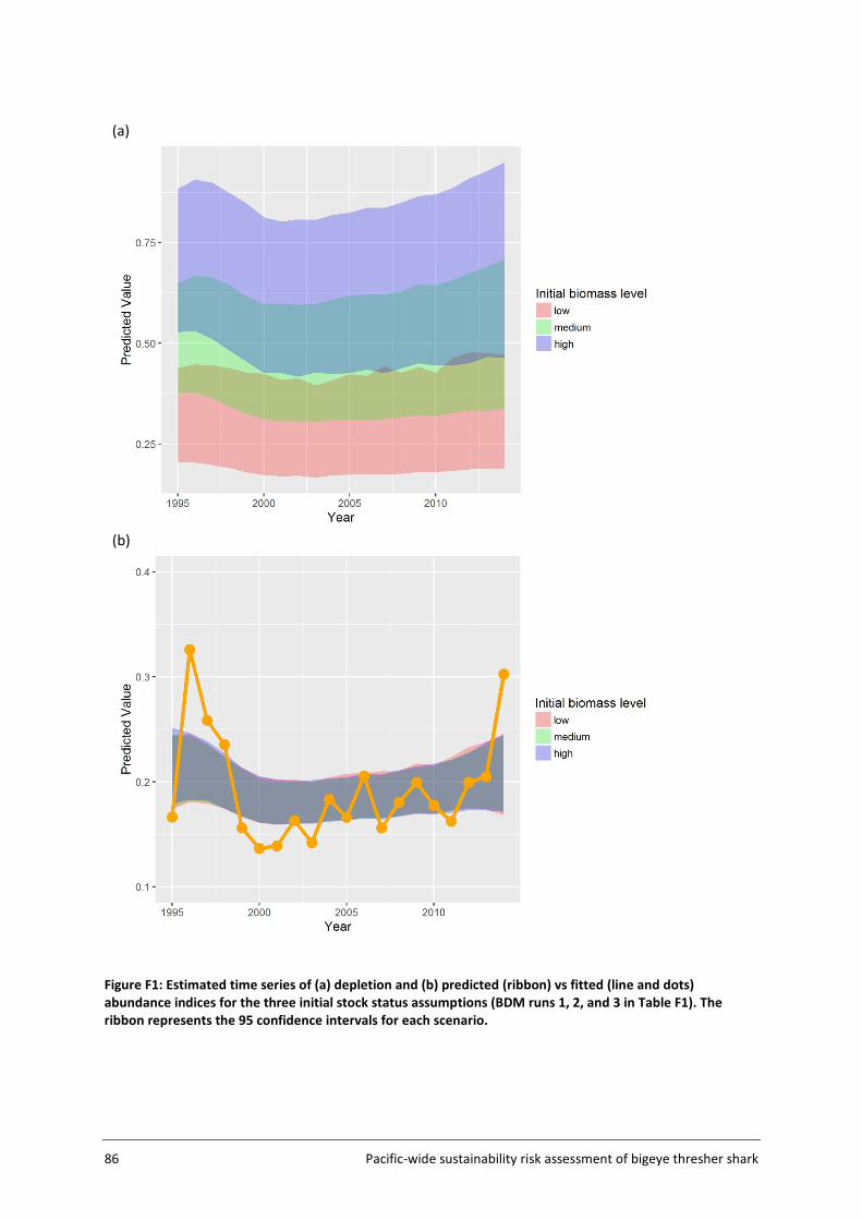
86 Pacific-wide sustainability risk assessment of bigeye thresher shark
(a)
(b)
Figure F1: Estimated time series of (a) depletion and (b) predicted (ribbon) vs fitted (line and dots) abundance indices for the three initial stock status assumptions (BDM runs 1, 2, and 3 in Table F1). The ribbon represents the 95 confidence intervals for each scenario.
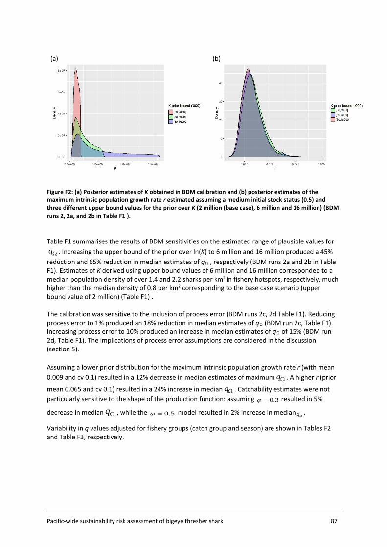
Pacific-wide sustainability risk assessment of bigeye thresher shark 87
(a)
(b)
Figure F2: (a) Posterior estimates of K obtained in BDM calibration and (b) posterior estimates of the maximum intrinsic population growth rate r estimated assuming a medium initial stock status (0.5) and three different upper bound values for the prior over K (2 million (base case), 6 million and 16 million) (BDM runs 2, 2a, and 2b in Table F1 ). Table F1 summarises the results of BDM sensitivities on the estimated range of plausible values for
Ωq . Increasing the upper bound of the prior over ln(K) to 6 million and 16 million produced a 45% reduction and 65% reduction in median estimates of qΩ , respectively (BDM runs 2a and 2b in Table F1). Estimates of K derived using upper bound values of 6 million and 16 million corresponded to a median population density of over 1.4 and 2.2 sharks per km2 in fishery hotspots, respectively, much higher than the median density of 0.8 per km2 corresponding to the base case scenario (upper bound value of 2 million) (Table F1) . The calibration was sensitive to the inclusion of process error (BDM runs 2c, 2d Table F1). Reducing process error to 1% produced an 18% reduction in median estimates of qΩ (BDM run 2c, Table F1). Increasing process error to 10% produced an increase in median estimates of qΩ of 15% (BDM run 2d, Table F1). The implications of process error assumptions are considered in the discussion (section 5). Assuming a lower prior distribution for the maximum intrinsic population growth rate r (with mean 0.009 and cv 0.1) resulted in a 12% decrease in median estimates of maximum Ωq . A higher r (prior
mean 0.065 and cv 0.1) resulted in a 24% increase in median Ωq . Catchability estimates were not particularly sensitive to the shape of the production function: assuming 3.0=ϕ resulted in 5%
decrease in median Ωq , while the 5.0=ϕ model resulted in 2% increase in medianΩq .
Variability in q values adjusted for fishery groups (catch group and season) are shown in Tables F2 and Table F3, respectively.
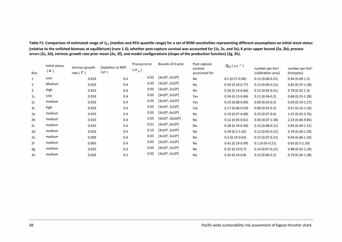
88 Pacific-wide sustainability risk assessment of bigeye thresher shark
Table F1: Comparison of estimated range of Ωq (median and 95% quantile range) for a set of BDM sensitivities representing different assumptions on initial stock status (relative to the unfished biomass at equilibrium) (runs 1-3); whether post-capture survival was accounted for (1s, 2s, and 3s); K prior upper bound (2a, 2b); process errors (2c, 2d), intrinsic growth rate prior mean (2e, 2f), and model configurations (shape of the production function) (2g, 2h).
Run
Initial status ( u )
Intrinsic growth rate ( r )
Depletion at MSY (ϕ )
Process error ( pσ )
Bounds of K prior Post-capture survival accounted for
Ωq ( 510− ) number per Km2
(calibration area) number per Km2
(hotspots)
1 Low 0.033 0.4 0.05 [3x10⁴, 2x10⁶] No 0.5 (0.27-0.96) 0.15 (0.08-0.21) 0.94 (0.49-1.3)
2 Medium 0.033 0.4 0.05 [3x10⁴, 2x10⁶] No 0.34 (0.19-0.77) 0.13 (0.06-0.21) 0.82 (0.37-1.28)
3 High 0.033 0.4 0.05 [3x10⁴, 2x10⁶] No 0.26 (0.14-0.66) 0.12 (0.05-0.21) 0.78 (0.32-1.3)
1s Low 0.033 0.4 0.05 [3x10⁴, 2x10⁶] Yes 0.34 (0.13-0.84) 0.11 (0.04-0.2) 0.68 (0.25-1.28)
2s medium 0.033 0.4 0.05 [3x10⁴, 2x10⁶] Yes 0.23 (0.08-0.69) 0.09 (0.03-0.2) 0.59 (0.19-1.27)
3s high 0.033 0.4 0.05 [3x10⁴, 2x10⁶] Yes 0.17 (0.06-0.59) 0.09 (0.03-0.2) 0.57 (0.16-1.26)
2a medium 0.033 0.4 0.05 [3x10⁴, 6x10⁶] No 0.19 (0.07-0.68) 0.23 (0.07-0.6) 1.41 (0.42-3.76)
2b medium 0.033 0.4 0.05 [3x10⁴, 16x106] No 0.12 (0.03-0.61) 0.36 (0.07-1.58) 2.23 (0.46-9.85)
2c medium 0.033 0.4 0.01 [3x10⁴, 2x10⁶] No 0.28 (0.18-0.58) 0.15 (0.08-0.21) 0.95 (0.49-1.31)
2d medium 0.033 0.4 0.10 [3x10⁴, 2x10⁶] No 0.39 (0.2-1.02) 0.12 (0.05-0.21) 0.76 (0.29-1.29)
2e medium 0.009 0.4 0.05 [3x10⁴, 2x10⁶] No 0.3 (0.19-0.63) 0.15 (0.07-0.21) 0.94 (0.46-1.29)
2f medium 0.065 0.4 0.05 [3x10⁴, 2x10⁶] No 0.42 (0.19-0.99) 0.1 (0.05-0.21) 0.63 (0.3-1.29)
2g medium 0.033 0.3 0.05 [3x10⁴, 2x10⁶] No 0.32 (0.19-0.7) 0.14 (0.07-0.21) 0.88 (0.42-1.29)
2h medium 0.033 0.5 0.05 [3x10⁴, 2x10⁶] No 0.35 (0.19-0.8) 0.13 (0.06-0.2) 0.79 (0.36-1.28)
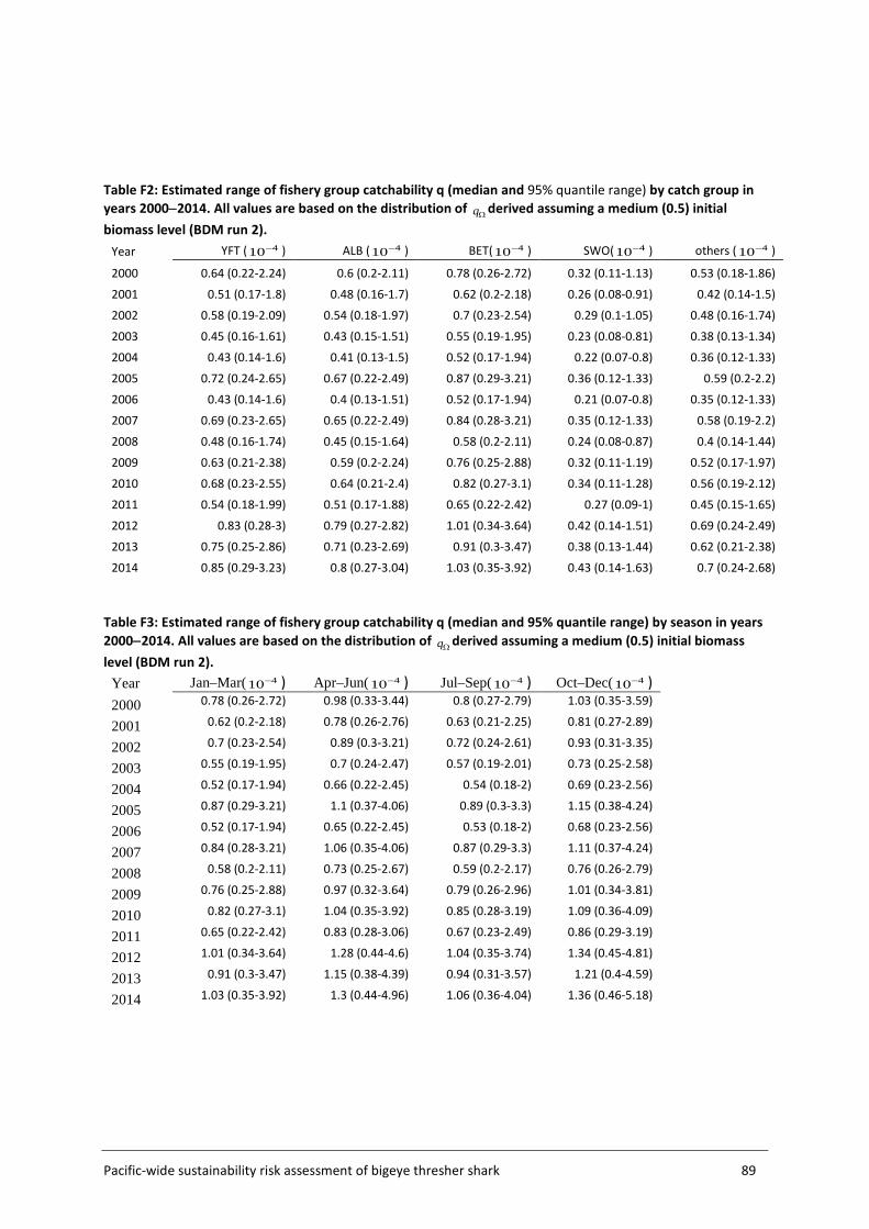
Pacific-wide sustainability risk assessment of bigeye thresher shark 89
Table F2: Estimated range of fishery group catchability q (median and 95% quantile range) by catch group in years 2000−2014. All values are based on the distribution of Ωq derived assuming a medium (0.5) initial biomass level (BDM run 2).
Year YFT ( 410− ) ALB ( 410− ) BET( 410− ) SWO( 410− ) others ( 410− )
2000 0.64 (0.22-2.24) 0.6 (0.2-2.11) 0.78 (0.26-2.72) 0.32 (0.11-1.13) 0.53 (0.18-1.86)
2001 0.51 (0.17-1.8) 0.48 (0.16-1.7) 0.62 (0.2-2.18) 0.26 (0.08-0.91) 0.42 (0.14-1.5)
2002 0.58 (0.19-2.09) 0.54 (0.18-1.97) 0.7 (0.23-2.54) 0.29 (0.1-1.05) 0.48 (0.16-1.74)
2003 0.45 (0.16-1.61) 0.43 (0.15-1.51) 0.55 (0.19-1.95) 0.23 (0.08-0.81) 0.38 (0.13-1.34)
2004 0.43 (0.14-1.6) 0.41 (0.13-1.5) 0.52 (0.17-1.94) 0.22 (0.07-0.8) 0.36 (0.12-1.33)
2005 0.72 (0.24-2.65) 0.67 (0.22-2.49) 0.87 (0.29-3.21) 0.36 (0.12-1.33) 0.59 (0.2-2.2)
2006 0.43 (0.14-1.6) 0.4 (0.13-1.51) 0.52 (0.17-1.94) 0.21 (0.07-0.8) 0.35 (0.12-1.33)
2007 0.69 (0.23-2.65) 0.65 (0.22-2.49) 0.84 (0.28-3.21) 0.35 (0.12-1.33) 0.58 (0.19-2.2)
2008 0.48 (0.16-1.74) 0.45 (0.15-1.64) 0.58 (0.2-2.11) 0.24 (0.08-0.87) 0.4 (0.14-1.44)
2009 0.63 (0.21-2.38) 0.59 (0.2-2.24) 0.76 (0.25-2.88) 0.32 (0.11-1.19) 0.52 (0.17-1.97)
2010 0.68 (0.23-2.55) 0.64 (0.21-2.4) 0.82 (0.27-3.1) 0.34 (0.11-1.28) 0.56 (0.19-2.12)
2011 0.54 (0.18-1.99) 0.51 (0.17-1.88) 0.65 (0.22-2.42) 0.27 (0.09-1) 0.45 (0.15-1.65)
2012 0.83 (0.28-3) 0.79 (0.27-2.82) 1.01 (0.34-3.64) 0.42 (0.14-1.51) 0.69 (0.24-2.49)
2013 0.75 (0.25-2.86) 0.71 (0.23-2.69) 0.91 (0.3-3.47) 0.38 (0.13-1.44) 0.62 (0.21-2.38)
2014 0.85 (0.29-3.23) 0.8 (0.27-3.04) 1.03 (0.35-3.92) 0.43 (0.14-1.63) 0.7 (0.24-2.68) Table F3: Estimated range of fishery group catchability q (median and 95% quantile range) by season in years 2000−2014. All values are based on the distribution of Ωq derived assuming a medium (0.5) initial biomass level (BDM run 2).
Year Jan–Mar( 410− ) Apr–Jun( 410− ) Jul–Sep( 410− ) Oct–Dec( 410− ) 2000 0.78 (0.26-2.72) 0.98 (0.33-3.44) 0.8 (0.27-2.79) 1.03 (0.35-3.59)
2001 0.62 (0.2-2.18) 0.78 (0.26-2.76) 0.63 (0.21-2.25) 0.81 (0.27-2.89)
2002 0.7 (0.23-2.54) 0.89 (0.3-3.21) 0.72 (0.24-2.61) 0.93 (0.31-3.35)
2003 0.55 (0.19-1.95) 0.7 (0.24-2.47) 0.57 (0.19-2.01) 0.73 (0.25-2.58)
2004 0.52 (0.17-1.94) 0.66 (0.22-2.45) 0.54 (0.18-2) 0.69 (0.23-2.56)
2005 0.87 (0.29-3.21) 1.1 (0.37-4.06) 0.89 (0.3-3.3) 1.15 (0.38-4.24)
2006 0.52 (0.17-1.94) 0.65 (0.22-2.45) 0.53 (0.18-2) 0.68 (0.23-2.56)
2007 0.84 (0.28-3.21) 1.06 (0.35-4.06) 0.87 (0.29-3.3) 1.11 (0.37-4.24)
2008 0.58 (0.2-2.11) 0.73 (0.25-2.67) 0.59 (0.2-2.17) 0.76 (0.26-2.79)
2009 0.76 (0.25-2.88) 0.97 (0.32-3.64) 0.79 (0.26-2.96) 1.01 (0.34-3.81)
2010 0.82 (0.27-3.1) 1.04 (0.35-3.92) 0.85 (0.28-3.19) 1.09 (0.36-4.09)
2011 0.65 (0.22-2.42) 0.83 (0.28-3.06) 0.67 (0.23-2.49) 0.86 (0.29-3.19)
2012 1.01 (0.34-3.64) 1.28 (0.44-4.6) 1.04 (0.35-3.74) 1.34 (0.45-4.81)
2013 0.91 (0.3-3.47) 1.15 (0.38-4.39) 0.94 (0.31-3.57) 1.21 (0.4-4.59)
2014 1.03 (0.35-3.92) 1.3 (0.44-4.96) 1.06 (0.36-4.04) 1.36 (0.46-5.18)
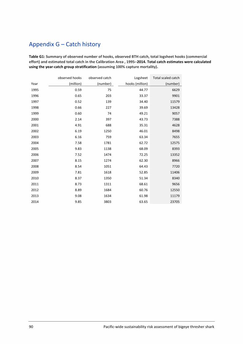
90 Pacific-wide sustainability risk assessment of bigeye thresher shark
Appendix G – Catch history Table G1: Summary of observed number of hooks, observed BTH catch, total logsheet hooks (commercial effort) and estimated total catch in the Calibration Area , 1995−2014. Total catch estimates were calculated using the year-catch group stratification (assuming 100% capture mortality).
observed hooks observed catch Logsheet Total scaled catch
Year (million) (number) hooks (million) (number)
1995 0.59 75 44.77 6629
1996 0.65 203 33.37 9901
1997 0.52 139 34.40 11579
1998 0.66 227 39.69 13428
1999 0.60 74 49.21 9057
2000 2.14 397 43.73 7388
2001 4.91 688 35.31 4628
2002 6.19 1250 46.01 8498
2003 6.16 759 63.34 7655
2004 7.58 1781 62.72 12575
2005 9.83 1138 68.09 8393
2006 7.52 1474 72.25 13352
2007 8.15 1274 62.30 8966
2008 8.54 1051 64.43 7720
2009 7.81 1618 52.85 11406
2010 8.37 1350 51.34 8340
2011 8.73 1311 68.61 9656
2012 8.89 1684 60.76 12550
2013 9.08 1634 61.98 11179
2014 9.85 3803 63.65 23705
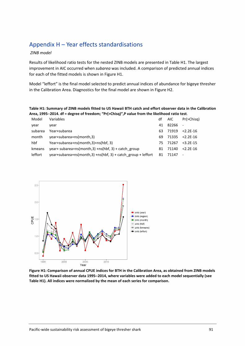
Pacific-wide sustainability risk assessment of bigeye thresher shark 91
Appendix H – Year effects standardisations ZINB model
Results of likelihood ratio tests for the nested ZINB models are presented in Table H1. The largest improvement in AIC occurred when subarea was included. A comparison of predicted annual indices for each of the fitted models is shown in Figure H1.
Model “leffort” is the final model selected to predict annual indices of abundance for bigeye thresher in the Calibration Area. Diagnostics for the final model are shown in Figure H2.
Table H1: Summary of ZINB models fitted to US Hawaii BTH catch and effort observer data in the Calibration Area, 1995−2014. df = degree of freedom; “Pr(>Chisq)”,P value from the likelihood ratio test.
Model Variables df AIC Pr(>Chisq) year year 41 82266 - subarea Year+subarea 63 71919 <2.2E-16 month year+subarea+ns(month,3) 69 71335 <2.2E-16 hbf Year+subarea+ns(month,3)+ns(hbf, 3) 75 71267 <3.2E-15 kmeans year+ subarea+ns(month,3) +ns(hbf, 3) + catch_group 81 71140 <2.2E-16 leffort year+subarea+ns(month,3) +ns(hbf, 3) + catch_group + leffort 81 71147 -
Figure H1: Comparison of annual CPUE indices for BTH in the Calibration Area, as obtained from ZINB models fitted to US Hawaii observer data 1995−2014, where variables were added to each model sequentially (see Table H1). All indices were normalized by the mean of each series for comparison.
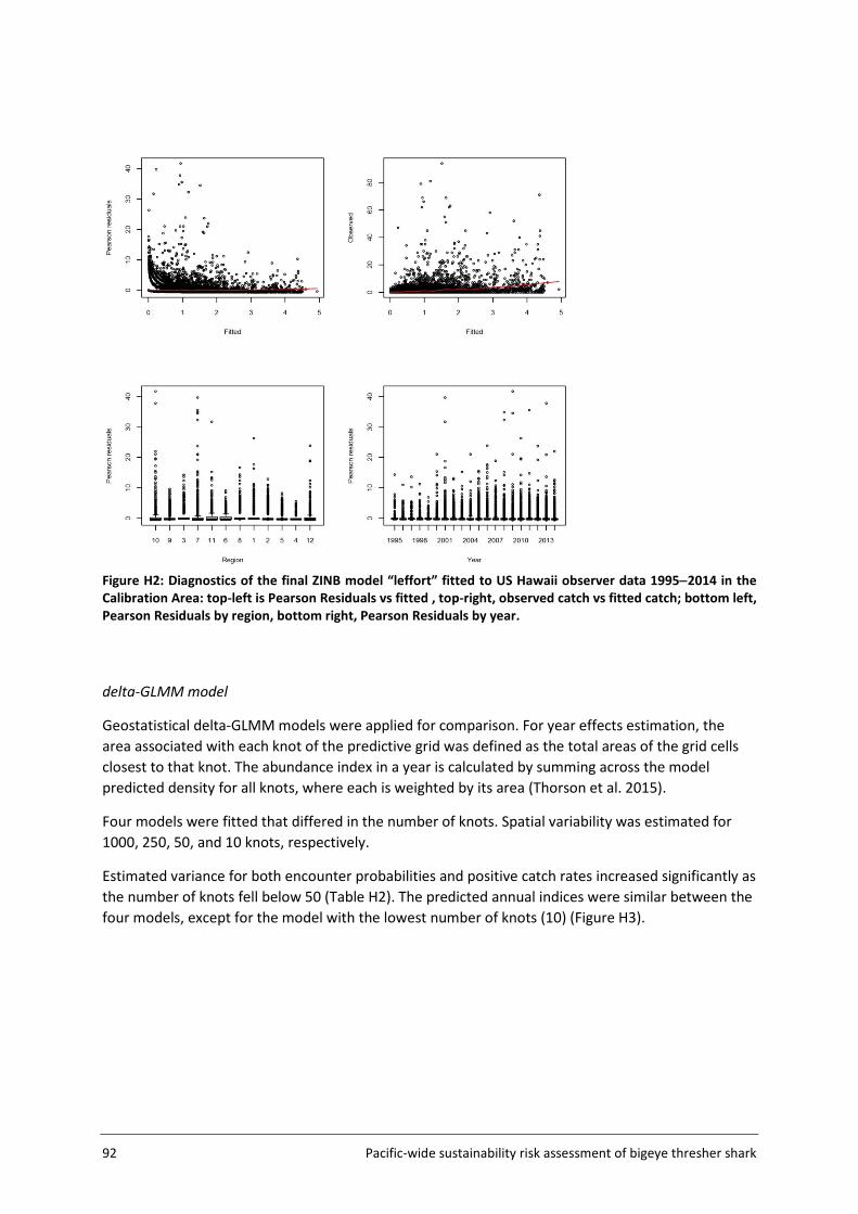
92 Pacific-wide sustainability risk assessment of bigeye thresher shark
Figure H2: Diagnostics of the final ZINB model “leffort” fitted to US Hawaii observer data 1995−2014 in the Calibration Area: top-left is Pearson Residuals vs fitted , top-right, observed catch vs fitted catch; bottom left, Pearson Residuals by region, bottom right, Pearson Residuals by year. delta-GLMM model
Geostatistical delta-GLMM models were applied for comparison. For year effects estimation, the area associated with each knot of the predictive grid was defined as the total areas of the grid cells closest to that knot. The abundance index in a year is calculated by summing across the model predicted density for all knots, where each is weighted by its area (Thorson et al. 2015).
Four models were fitted that differed in the number of knots. Spatial variability was estimated for 1000, 250, 50, and 10 knots, respectively.
Estimated variance for both encounter probabilities and positive catch rates increased significantly as the number of knots fell below 50 (Table H2). The predicted annual indices were similar between the four models, except for the model with the lowest number of knots (10) (Figure H3).
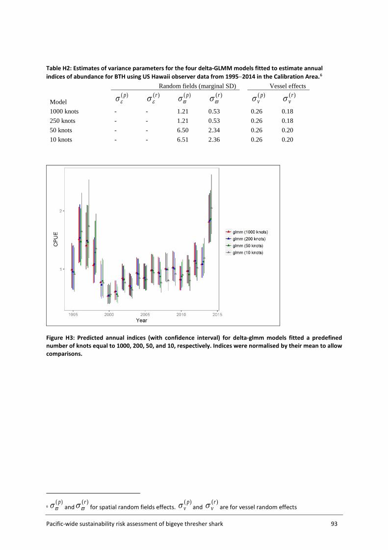
Pacific-wide sustainability risk assessment of bigeye thresher shark 93
Table H2: Estimates of variance parameters for the four delta-GLMM models fitted to estimate annual indices of abundance for BTH using US Hawaii observer data from 1995−2014 in the Calibration Area.6
Random fields (marginal SD) Vessel effects
Model )( p
εσ )(r
εσ )( p
ϖσ )(r
ϖσ )( p
vσ )(r
vσ
1000 knots - - 1.21 0.53 0.26 0.18 250 knots - - 1.21 0.53 0.26 0.18 50 knots - - 6.50 2.34 0.26 0.20 10 knots - - 6.51 2.36 0.26 0.20
Figure H3: Predicted annual indices (with confidence interval) for delta-glmm models fitted a predefined number of knots equal to 1000, 200, 50, and 10, respectively. Indices were normalised by their mean to allow comparisons.
6 )( p
ϖσ and)(r
ϖσ for spatial random fields effects. )( p
vσ and )(r
vσ are for vessel random effects
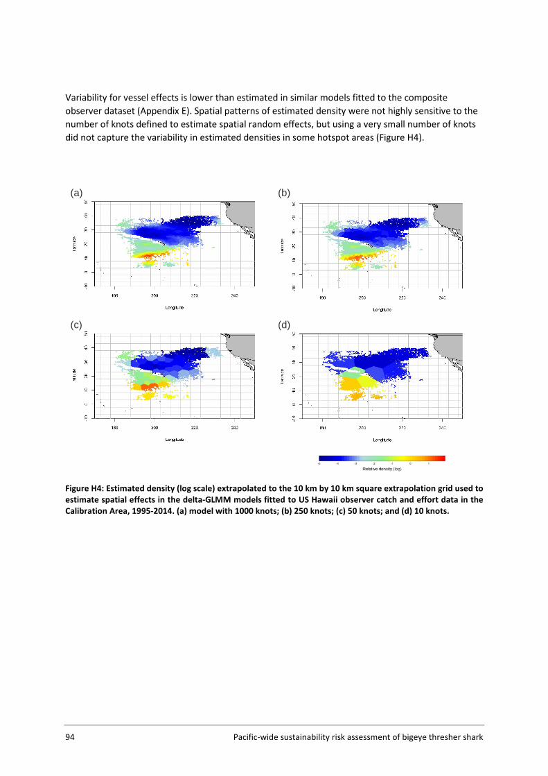
94 Pacific-wide sustainability risk assessment of bigeye thresher shark
Variability for vessel effects is lower than estimated in similar models fitted to the composite observer dataset (Appendix E). Spatial patterns of estimated density were not highly sensitive to the number of knots defined to estimate spatial random effects, but using a very small number of knots did not capture the variability in estimated densities in some hotspot areas (Figure H4).
(a)
(b)
(c)
(d)
Figure H4: Estimated density (log scale) extrapolated to the 10 km by 10 km square extrapolation grid used to estimate spatial effects in the delta-GLMM models fitted to US Hawaii observer catch and effort data in the Calibration Area, 1995-2014. (a) model with 1000 knots; (b) 250 knots; (c) 50 knots; and (d) 10 knots.
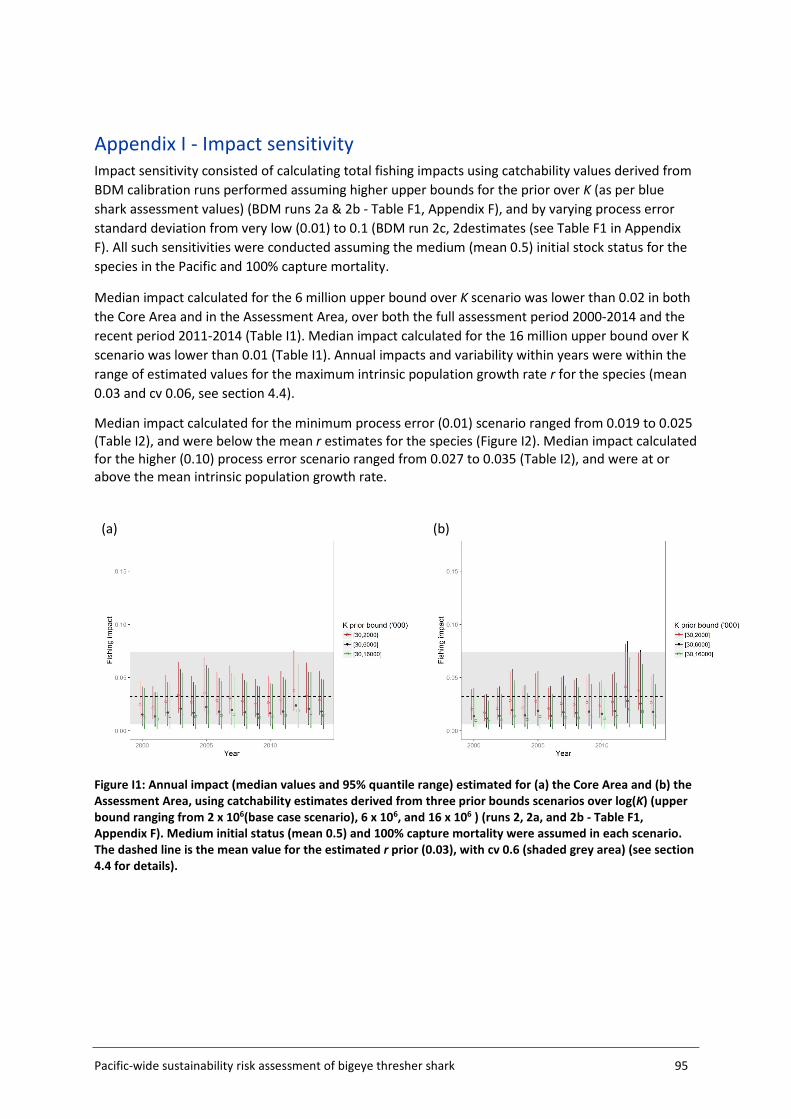
Pacific-wide sustainability risk assessment of bigeye thresher shark 95
Appendix I - Impact sensitivity Impact sensitivity consisted of calculating total fishing impacts using catchability values derived from BDM calibration runs performed assuming higher upper bounds for the prior over K (as per blue shark assessment values) (BDM runs 2a & 2b - Table F1, Appendix F), and by varying process error standard deviation from very low (0.01) to 0.1 (BDM run 2c, 2destimates (see Table F1 in Appendix F). All such sensitivities were conducted assuming the medium (mean 0.5) initial stock status for the species in the Pacific and 100% capture mortality.
Median impact calculated for the 6 million upper bound over K scenario was lower than 0.02 in both the Core Area and in the Assessment Area, over both the full assessment period 2000-2014 and the recent period 2011-2014 (Table I1). Median impact calculated for the 16 million upper bound over K scenario was lower than 0.01 (Table I1). Annual impacts and variability within years were within the range of estimated values for the maximum intrinsic population growth rate r for the species (mean 0.03 and cv 0.06, see section 4.4).
Median impact calculated for the minimum process error (0.01) scenario ranged from 0.019 to 0.025 (Table I2), and were below the mean r estimates for the species (Figure I2). Median impact calculated for the higher (0.10) process error scenario ranged from 0.027 to 0.035 (Table I2), and were at or above the mean intrinsic population growth rate.
(a)
(b)
Figure I1: Annual impact (median values and 95% quantile range) estimated for (a) the Core Area and (b) the Assessment Area, using catchability estimates derived from three prior bounds scenarios over log(K) (upper bound ranging from 2 x 10⁶(base case scenario), 6 x 10⁶, and 16 x 106 ) (runs 2, 2a, and 2b - Table F1, Appendix F). Medium initial status (mean 0.5) and 100% capture mortality were assumed in each scenario. The dashed line is the mean value for the estimated r prior (0.03), with cv 0.6 (shaded grey area) (see section 4.4 for details).
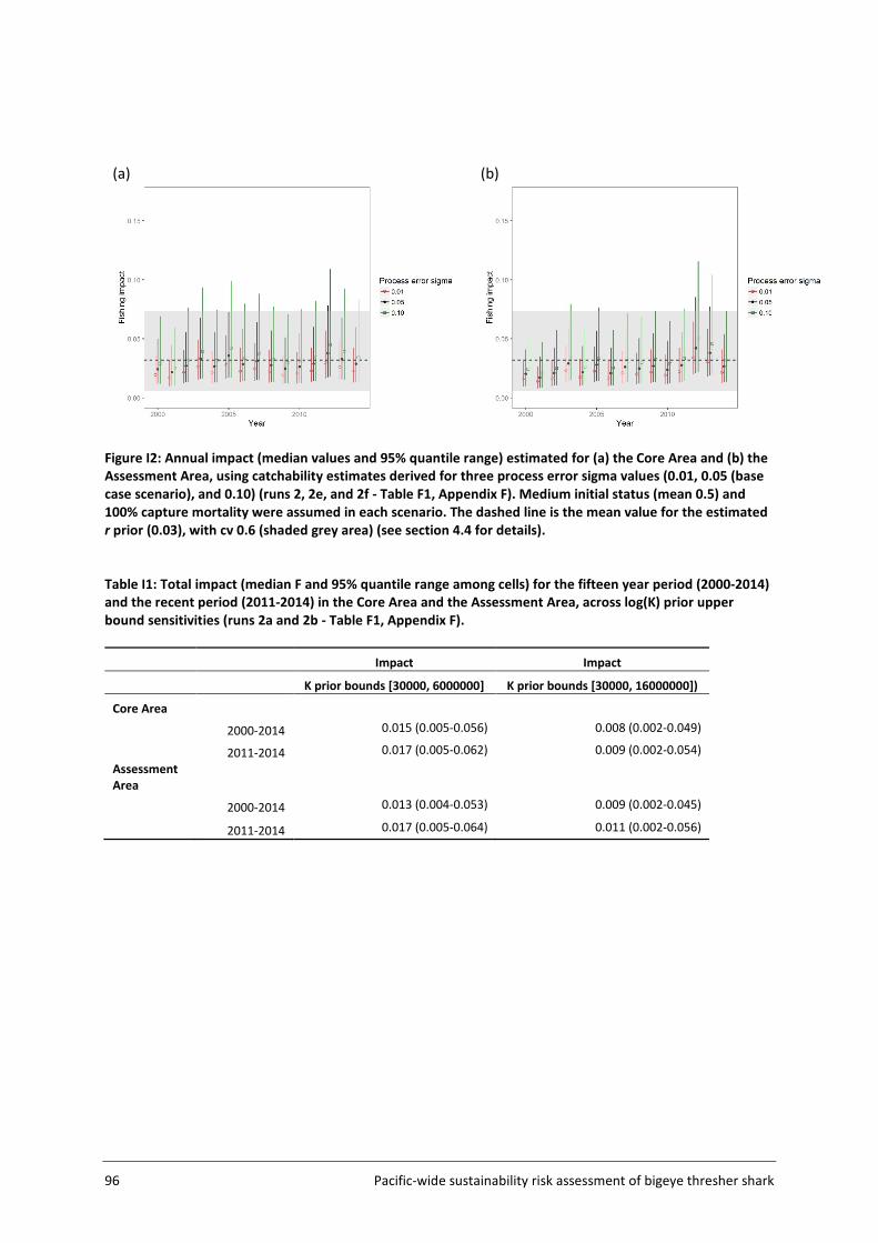
96 Pacific-wide sustainability risk assessment of bigeye thresher shark
(a)
(b)
Figure I2: Annual impact (median values and 95% quantile range) estimated for (a) the Core Area and (b) the Assessment Area, using catchability estimates derived for three process error sigma values (0.01, 0.05 (base case scenario), and 0.10) (runs 2, 2e, and 2f - Table F1, Appendix F). Medium initial status (mean 0.5) and 100% capture mortality were assumed in each scenario. The dashed line is the mean value for the estimated r prior (0.03), with cv 0.6 (shaded grey area) (see section 4.4 for details). Table I1: Total impact (median F and 95% quantile range among cells) for the fifteen year period (2000-2014) and the recent period (2011-2014) in the Core Area and the Assessment Area, across log(K) prior upper bound sensitivities (runs 2a and 2b - Table F1, Appendix F).
Impact Impact
K prior bounds [30000, 6000000] K prior bounds [30000, 16000000])
Core Area
2000-2014 0.015 (0.005-0.056) 0.008 (0.002-0.049)
2011-2014 0.017 (0.005-0.062) 0.009 (0.002-0.054) Assessment Area
2000-2014 0.013 (0.004-0.053) 0.009 (0.002-0.045)
2011-2014 0.017 (0.005-0.064) 0.011 (0.002-0.056)
Pacific-wide sustainability risk assessment of bigeye thresher shark 97
Table I2: Total impact (median F and 95% quantile range among cells) for the fifteen year period (2000-2014) and the recent period (2011-2014) in the Core Area and the Assessment Area, across process error sensitivities (runs 2c and 2d - Table F1, Appendix F).
Impact Impact
Process error sigma 0.01 Process error sigma 0.10
Core Area
2000-2014 0.021 (0.012-0.045) 0.029 (0.013-0.085)
2011-2014 0.023 (0.014-0.049) 0.033 (0.015-0.093) Assessment Area
2000-2014 0.019 (0.01-0.045) 0.027 (0.012-0.077)
2011-2014 0.025 (0.013-0.056) 0.035 (0.015-0.097)
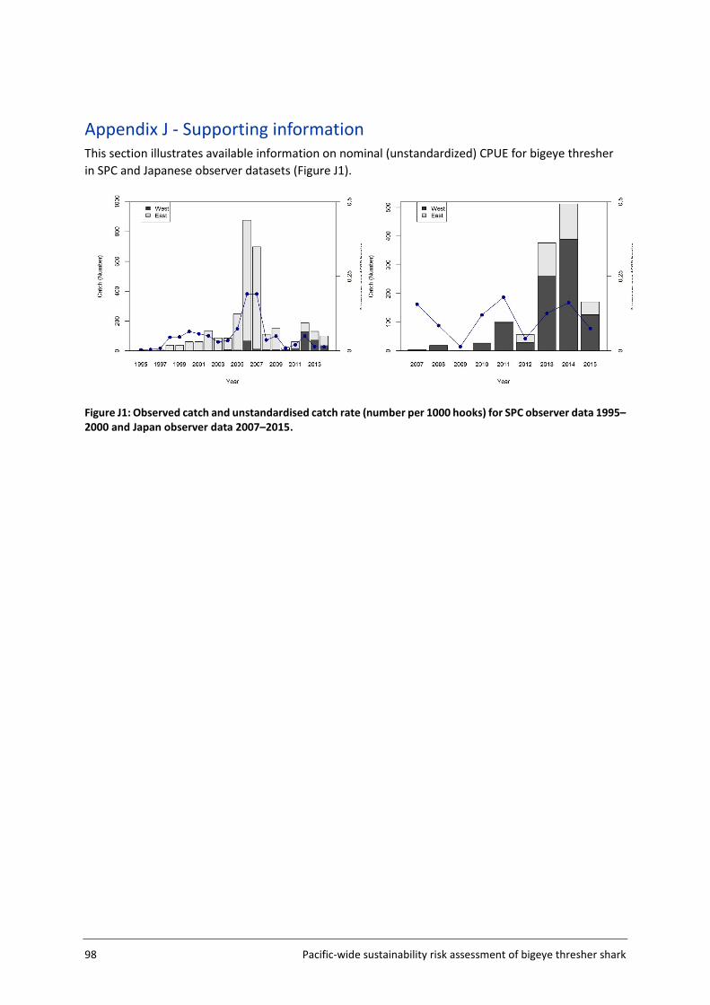
98 Pacific-wide sustainability risk assessment of bigeye thresher shark
Appendix J - Supporting information This section illustrates available information on nominal (unstandardized) CPUE for bigeye thresher in SPC and Japanese observer datasets (Figure J1).
Figure J1: Observed catch and unstandardised catch rate (number per 1000 hooks) for SPC observer data 1995–2000 and Japan observer data 2007–2015.


![CMM 2008-01 [Bigeye and Yellowfin] CONSERVATION AND MANAGEMENT MEASURE FOR BIGEYE AND YELLOWFIN TUNA IN THE WESTERN AND CENTRAL PACIFIC OCEAN Conservation and Management Measure 2008-01](https://img.pdfslide.net/doc/110x75/55cf995c550346d0339cfa56/cmm-2008-01-bigeye-and-yellowfin-conservation-and-management-measure-for.jpg)


![SCIENTIFIC COMMITTEE TENTH REGULAR SESSION … [BET Assessment]_rev1... · STOCK ASSESSMENT OF BIGEYE TUNA IN THE WESTERN AND CENTRAL PACIFIC OCEAN ... 1 Introduction ... , but should](https://img.pdfslide.net/doc/110x75/5b5c7a1d7f8b9a68368cd900/scientific-committee-tenth-regular-session-bet-assessmentrev1-stock-assessment.jpg)