Package ‘lawstat’ - The Comprehensive R Archive … 5 Arguments x the numeric vector of data values from the sample 1. y the numeric vector of data values from the sample 2. alpha

Package ‘lawstat’November 23, 2017

Type Package

Title Tools for Biostatistics, Public Policy, and Law

Version 3.2

Date 2017-11-22

Depends R (>= 2.6.0), Kendall, mvtnorm, VGAM

Suggests fBasics

License GPL (>= 2)

DescriptionStatistical tests widely utilized in biostatistics, public policy, and law. Along with the well-known tests for equality of means and variances, randomness,measures of relative variability etc, the package contains new robust tests of symmetry,omnibus and directional tests of normality, and their graphical counterparts such asRobust QQ plot; a robust trend tests for variances etc. All implemented tests and methodsare illustrated by simulations and real-life examples from legal statistics, economics,and biostatistics.

NeedsCompilation no

Author Joseph L. Gastwirth [aut],Yulia R. Gel [aut],W. L. Wallace Hui [aut],Vyacheslav Lyubchich [aut, cre],Weiwen Miao [aut],Kimihiro Noguchi [aut]

Maintainer Vyacheslav Lyubchich <[email protected]>

Repository CRAN

Date/Publication 2017-11-23 14:01:33 UTC

R topics documented:bartels.test . . . . . . . . . . . . . . . . . . . . . . . . . . . . . . . . . . . . . . . . . . 2bias . . . . . . . . . . . . . . . . . . . . . . . . . . . . . . . . . . . . . . . . . . . . . 3blackhire . . . . . . . . . . . . . . . . . . . . . . . . . . . . . . . . . . . . . . . . . . 4brunner.munzel.test . . . . . . . . . . . . . . . . . . . . . . . . . . . . . . . . . . . . . 4

1

2 bartels.test

cd . . . . . . . . . . . . . . . . . . . . . . . . . . . . . . . . . . . . . . . . . . . . . . 6cmh.test . . . . . . . . . . . . . . . . . . . . . . . . . . . . . . . . . . . . . . . . . . . 7data1963 . . . . . . . . . . . . . . . . . . . . . . . . . . . . . . . . . . . . . . . . . . . 9gini.index . . . . . . . . . . . . . . . . . . . . . . . . . . . . . . . . . . . . . . . . . . 10j.maad . . . . . . . . . . . . . . . . . . . . . . . . . . . . . . . . . . . . . . . . . . . . 11laplace.test . . . . . . . . . . . . . . . . . . . . . . . . . . . . . . . . . . . . . . . . . 12levene.test . . . . . . . . . . . . . . . . . . . . . . . . . . . . . . . . . . . . . . . . . . 13lnested.test . . . . . . . . . . . . . . . . . . . . . . . . . . . . . . . . . . . . . . . . . 16lorenz.curve . . . . . . . . . . . . . . . . . . . . . . . . . . . . . . . . . . . . . . . . . 19ltrend.test . . . . . . . . . . . . . . . . . . . . . . . . . . . . . . . . . . . . . . . . . . 21michigan . . . . . . . . . . . . . . . . . . . . . . . . . . . . . . . . . . . . . . . . . . 24mma.test . . . . . . . . . . . . . . . . . . . . . . . . . . . . . . . . . . . . . . . . . . . 25neuhauser.hothorn.test . . . . . . . . . . . . . . . . . . . . . . . . . . . . . . . . . . . 26nig.parameter . . . . . . . . . . . . . . . . . . . . . . . . . . . . . . . . . . . . . . . . 29popdata . . . . . . . . . . . . . . . . . . . . . . . . . . . . . . . . . . . . . . . . . . . 30pot . . . . . . . . . . . . . . . . . . . . . . . . . . . . . . . . . . . . . . . . . . . . . . 31rjb.test . . . . . . . . . . . . . . . . . . . . . . . . . . . . . . . . . . . . . . . . . . . . 32rlm.test . . . . . . . . . . . . . . . . . . . . . . . . . . . . . . . . . . . . . . . . . . . 33robust.mmm.test . . . . . . . . . . . . . . . . . . . . . . . . . . . . . . . . . . . . . . 35rqq . . . . . . . . . . . . . . . . . . . . . . . . . . . . . . . . . . . . . . . . . . . . . . 36runs.test . . . . . . . . . . . . . . . . . . . . . . . . . . . . . . . . . . . . . . . . . . . 38sj.test . . . . . . . . . . . . . . . . . . . . . . . . . . . . . . . . . . . . . . . . . . . . 40symmetry.test . . . . . . . . . . . . . . . . . . . . . . . . . . . . . . . . . . . . . . . . 41zuni . . . . . . . . . . . . . . . . . . . . . . . . . . . . . . . . . . . . . . . . . . . . . 43

Index 44

bartels.test Ranked Version of von Neumann’s Ratio Test for Randomness

Description

This function performs the Bartels test for randomness which is based on the ranked version of vonNeumann’s ratio (RVN). Users can choose whether to test against two-sided, negative or positivecorrelation. NAs from the data are omitted.

Usage

bartels.test(y, alternative = c("two.sided", "positive.correlated","negative.correlated"))

Arguments

y a numeric vector of data values.

alternative a character string specifying the alternative hypothesis, must be one of "two.sided"(default), "negative.correlated", or "positive.correlated".

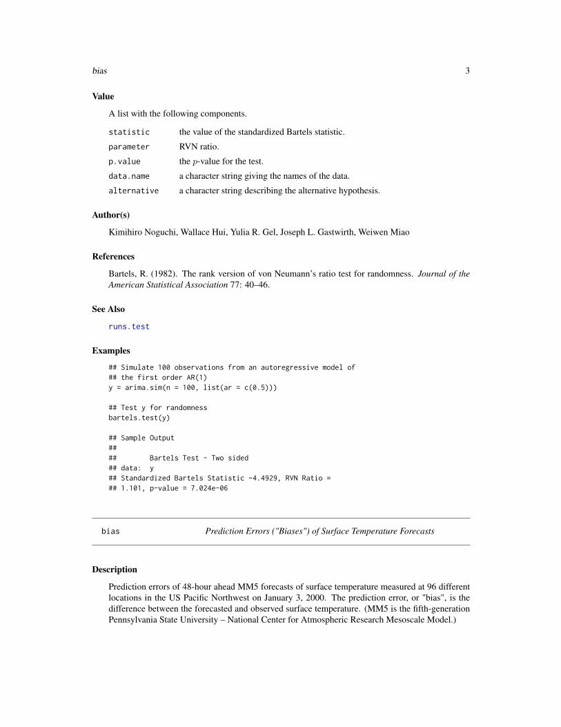
bias 3

Value

A list with the following components.

statistic the value of the standardized Bartels statistic.

parameter RVN ratio.

p.value the p-value for the test.

data.name a character string giving the names of the data.

alternative a character string describing the alternative hypothesis.

Author(s)

Kimihiro Noguchi, Wallace Hui, Yulia R. Gel, Joseph L. Gastwirth, Weiwen Miao

References

Bartels, R. (1982). The rank version of von Neumann’s ratio test for randomness. Journal of theAmerican Statistical Association 77: 40–46.

See Also

runs.test

Examples

## Simulate 100 observations from an autoregressive model of## the first order AR(1)y = arima.sim(n = 100, list(ar = c(0.5)))

## Test y for randomnessbartels.test(y)

## Sample Output#### Bartels Test - Two sided## data: y## Standardized Bartels Statistic -4.4929, RVN Ratio =## 1.101, p-value = 7.024e-06

bias Prediction Errors ("Biases") of Surface Temperature Forecasts

Description

Prediction errors of 48-hour ahead MM5 forecasts of surface temperature measured at 96 differentlocations in the US Pacific Northwest on January 3, 2000. The prediction error, or "bias", is thedifference between the forecasted and observed surface temperature. (MM5 is the fifth-generationPennsylvania State University – National Center for Atmospheric Research Mesoscale Model.)

4 brunner.munzel.test

Usage

bias

Source

Data have been kindly provided by the research group of Professor Clifford Mass in the De-partment of Atmospheric Sciences at the University of Washington. Detailed information aboutthe Pacific Northwest prediction effort and the associated data archive can be found online atwww.atmos.washington.edu/mm5rt/info.html and www.atmos.washington.edu/marka/pnw.html, respectively.

blackhire Hiring data for eight professions and two races

Description

Number of black and white candidates (hired or rejected) for eight professions.

Usage

blackhire

Format

An array with 2 rows by 2 columns by 8 levels.

References

Gastwirth, J. L. (1984). Statistical methods for analyzing claims of employment discrimination.Industrial and Labor Relations Review 38(1): 75–86.

brunner.munzel.test The Brunner–Munzel Test for Stochastic Equality

Description

This function performs the Brunner–Munzel test for stochastic equality of two samples, which isalso known as the Generalized Wilcoxon Test. NAs from the data are omitted.

Usage

brunner.munzel.test(x, y, alternative = c("two.sided", "greater","less"), alpha = 0.05)

www.atmos.washington.edu/mm5rt/info.html

www.atmos.washington.edu/marka/pnw.html

www.atmos.washington.edu/marka/pnw.html

brunner.munzel.test 5

Arguments

x the numeric vector of data values from the sample 1.

y the numeric vector of data values from the sample 2.

alpha significance level, default is 0.05 for 95% confidence interval.

alternative a character string specifying the alternative hypothesis, must be one of "two.sided"(default), "greater" or "less". User can specify just the initial letter.

Value

A list containing the following components:

statistic the Brunner–Munzel test statistic.

parameter the degrees of freedom.

conf.int the confidence interval.

p.value the p-value of the test.

data.name a character string giving the name of the data.

estimate an estimate of the effect size, i.e., P (X < Y ) + 0.5 ∗ P (X = Y )

Note

There exist discrepancies with Brunner and Munzel (2000) because there is a typo in the paper. Thecorrected version is in Neubert and Brunner (2007) (e.g., compare the estimates for the case studyon pain scores). The current R function follows Neubert and Brunner (2007).

Author(s)

Wallace Hui, Yulia R. Gel, Joseph L. Gastwirth, Weiwen Miao. This function was updated with thehelp of Dr. Ian Fellows

References

Brunner, E. and Munzel, U. (2000). The nonparametric Behrens-Fisher problem: asymptotic theoryand a small-sample approximation. Biometrical Journal 42: 17–25.

Neubert, K. and Brunner, E. (2007). A Studentized permutation test for the non-parametric Behrens-Fisher problem. Computational Statistics and Data Analysis 51: 5192–5204.

Reiczigel, J., Zakarias, I., and Rozsa, L. (2005). A bootstrap test of stochastic equality of twopopulations. The American Statistician 59: 1–6.

See Also

wilcox.test, pwilcox

6 cd

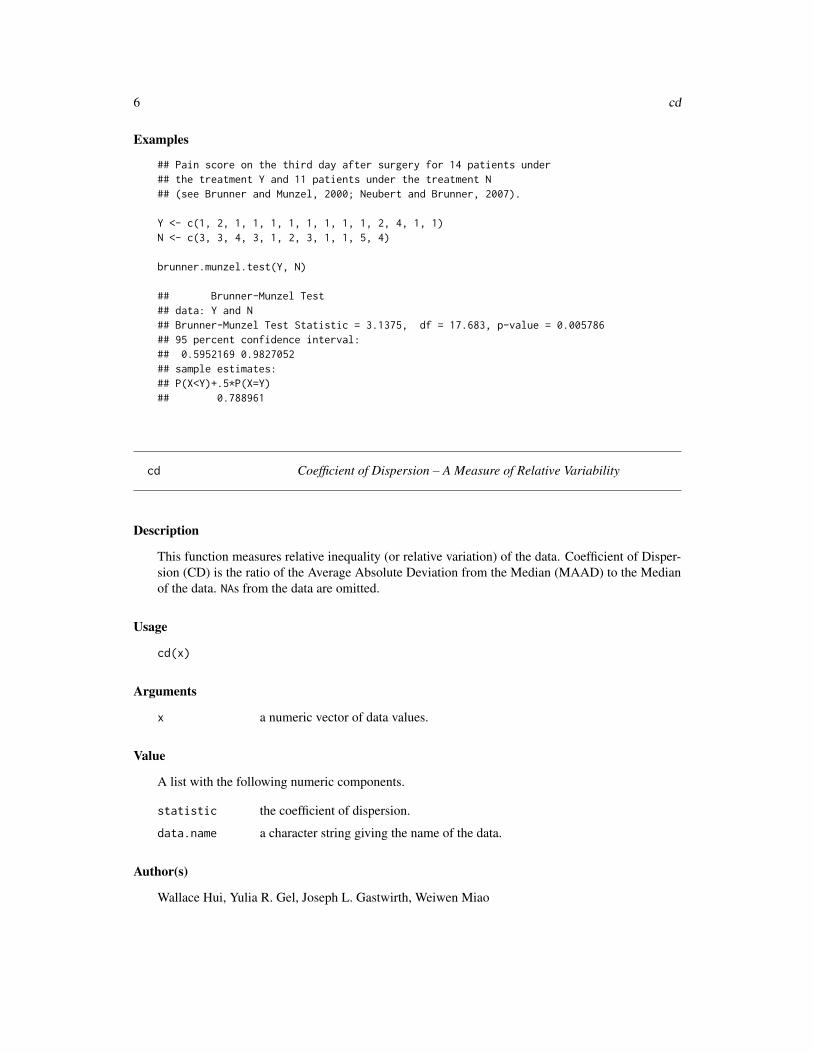
Examples

## Pain score on the third day after surgery for 14 patients under## the treatment Y and 11 patients under the treatment N## (see Brunner and Munzel, 2000; Neubert and Brunner, 2007).

Y <- c(1, 2, 1, 1, 1, 1, 1, 1, 1, 1, 2, 4, 1, 1)N <- c(3, 3, 4, 3, 1, 2, 3, 1, 1, 5, 4)

brunner.munzel.test(Y, N)

## Brunner-Munzel Test## data: Y and N## Brunner-Munzel Test Statistic = 3.1375, df = 17.683, p-value = 0.005786## 95 percent confidence interval:## 0.5952169 0.9827052## sample estimates:## P(X<Y)+.5*P(X=Y)## 0.788961

cd Coefficient of Dispersion – A Measure of Relative Variability

Description

This function measures relative inequality (or relative variation) of the data. Coefficient of Disper-sion (CD) is the ratio of the Average Absolute Deviation from the Median (MAAD) to the Medianof the data. NAs from the data are omitted.

Usage

cd(x)

Arguments

x a numeric vector of data values.

Value

A list with the following numeric components.

statistic the coefficient of dispersion.


Author(s)

Wallace Hui, Yulia R. Gel, Joseph L. Gastwirth, Weiwen Miao

cmh.test 7

References

Bonett, D. G. and Seier, E. (2005). Confidence interval for a coefficient of dispersion in nonnormaldistributions. Biometrical Journal 48(1): 144–148.

Gastwirth, J. L. (1988). Statistical Reasoning in Law and Public Policy Vol 1. Academic Press,Boston, Toronto.

See Also

gini.index, j.maad

Examples

## The Baker v. Carr Case: one-person-one-vote decision.## Measure of Relative Inequality of Population data in 33 districts## of the Tennessee Legislature in 1900 and 1972. See## popdata (see Gastwirth, 1988).

data(popdata)cd(popdata[,"pop1900"])

## Measures of Relative Variability - Coefficient of Dispersion#### data: popdata[, "pop1900"]## Coefficient of Dispersion = 0.1673

cd(popdata[,"pop1972"])

## Measures of Relative Variability - Coefficient of Dispersion#### data: popdata[, "pop1972"]## Coefficient of Dispersion = 0.0081

cmh.test The Cochran-Mantel-Haenszel Chi-square Test

Description

This function performs the Cochran-Mantel-Haenszel (CMH) procedure. The CMH procedure testshomogeneity of population proportions after taking into account other factors. This procedure iswidely used in various law cases, in particular, on equal employment and discrimination, as well inbiological and phamaceutical studies.

Usage

cmh.test(x)

Arguments

x a numeric 2 x 2 x k array of data values.

8 cmh.test

Details

The test is based on the CMH procedure discussed by Gastwirth, 1984. The data should be inputin a array of 2 rows x 2 columns x k levels. The output includes the Mantel-Haenszel Estimate, thepooled Odd Ratio, and the Odd Ratio between the rows and columns at each level. The Chi-squareTest of Significance tests if there is an interaction or association between rows and columns.

The null hypothesis is that the pooled Odd Ratio is equal to 1, i.e., there is no interaction betweenrows and columns. For more details see Gastwirth (1984).

Notice that cmh.test can be viewed as a subset of mantelhaen.test, in the sense that cmh.test is fora 2 by 2 by k table without continuity correction whereas mantelhaen.test allows for a larger table,and for a 2 by 2 by k table, it has an option of performing continuity correction or not. However, inview of Gastwirth (1984), continuity correction is not recommended as it tends to overestimate thep-value.

Value

A list with class htest containing the following components:

MH.ESTIMATE the value of the Cochran-Mantel-Haenszel Estimate.

OR Pooled Odd Ratio of the data.

ORK vector of Odd Ratio of each level

cmh the test statistic.

df degrees of freedom.


method type of test was performed.


Author(s)

Min Qin, Wallace W. Hui, Yulia R. Gel, Joseph L. Gastwirth

References

Gastwirth, J. L.(1984) Statistical Methods for Analyzing Claims of Employment Discrimination,Industrial and Labor Relations Review, Vol. 38, No. 1. (October 1984), pp. 75-86.

See Also

mantelhaen.test

Examples

## Sample Salary Data

data(blackhire)cmh.test(blackhire)

data1963 9

## Sample Output#### Mantel-Haenszel Chi-square Test#### data: blackhire## Mantel-Haenszel Estimate = 0.477, Chi-squared = 145.840, df = 1.000, p-value = 0.000,## Pooled Odd Ratio = 0.639, Odd Ratio of level 1 = 1.329, Odd Ratio of level 2 = 0.378, Odd## Ratio of level 3 = 0.508, Odd Ratio of level 4 = 0.357, Odd Ratio of level 5 = 0.209, Odd## Ratio of level 6 = 0.412, Odd Ratio of level 7 = 0.250, Odd Ratio of level 8 = 0.820#### Note: P-value is significant and we should reject the null hypothesis.

data1963 Population data of ratio of number of senators and representatives topopulation size in 1963

Description

The dataset of ratio of number of senators and representatives to population size in 13 districts inthe United States in 1963 (Gastwirth, 1972).

Usage

data1963

Format

A data frame with 13 observations on the following 3 variables.

pop1963 population data in 1963

sen1963 Number of senators in each district in 1963

rep1963 Number of representatives in each district in 1963

Source

Gastwirth, J. L.(1972) The Estimation of the Lorenz Curve and Gini Index, The Review of Eco-nomics and Statistics, Vol. 54, No. 3. (August 1972), pp. 306-316.

References


10 gini.index

gini.index Measures of Relative Variability - Gini Index

Description

This function measures relative inequality (or relative variation) of the data using the Gini Index.NAs from the data are omitted.

Usage

gini.index(x)

Arguments

x the input data.

Value


statistic The Gini Index of the data.

parameter the mean difference of a set of numbers.


Author(s)


References

Gastwirth, J. L.(1988) Statistical Reasoning in Law and Public Policy Vol 1, Boston; Toronto, Aca-demic Press.

Gini, C. Variabilita e mutabilita (1912) Reprinted in Memorie di metodologica statistica (Ed. PizettiE, Salvemini, T. Rome: Libreria Eredi Virgilio Veschi (1955). English translation in Metron,2005,63,(1) 3-38

See Also

cd, j.maad, lorenz.curve

j.maad 11

Examples

## The Baker v. Carr Case: one-person-one-vote decision.## Measure of Relative Inequality of Population data in 33 districts## of the Tennessee Legislature in 1900 and 1972. See## popdata (see Gastwirth (1988)).

data(popdata)gini.index(popdata[,"pop1900"])

## Measures of Relative Variability - Gini Index#### data: popdata[, "pop1900"]## Gini Index = 0.1147, delta = 3389.765

gini.index(popdata[,"pop1972"])

## Measures of Relative Variability - Gini Index#### data: popdata[, "pop1972"]## Gini Index = 0.0055, delta = 1297.973

j.maad MAAD estimated Robust Standard Deviation

Description

This function computes the average absolute deviation from the sample median, which is a consis-tent robust estimate of the population standard deviation for normality distribution data. NAs fromthe data are omitted.

Usage

j.maad(x)

Arguments


Value


J Robust Standard Deviation J

Author(s)


12 laplace.test

References

Gastwirth, J. L.(1982) Statistical Properties of A Measure of Tax Assessment Uniformity, Journal ofStatistical Planning and Inference 6, 1-12.

See Also

cd, gini.index, rqq, rjb.test, sj.test

Examples

## Simulate 100 observations: using rnorm()## for normally distributed data, X=N(0,1)x = rnorm(100)j.maad(x)

## Sample Output#### MAAD estimated J = 0.9194124302405 for data x

laplace.test Goodness-of-fit tests for the Laplace distribution

Description

The function returns five goodness-of-fit test statistics for the Laplace distribution. The four statis-tics are: A2 (Anderson-Darling), W2 (Cramer-von Mises), U2 (Watson), D (Kolmogorov-Smirnov),and V (Kuiper). By default, NAs are omitted. This function requires the VGAM package.

Usage

laplace.test(y)

Arguments


Value


A2 the Anderson-Darling statistic.

W2 the Cramer-von Mises statistic.

U2 the Watson statistic.

D the Kolmogorov-Smirnov statistic.

V the Kuiper statistic.

levene.test 13

Author(s)

Kimihiro Noguchi, Yulia R. Gel

References

Puig, P. and Stephens, M. A. (2000). Tests of fit for the Laplace distribution, with applications.Technometrics 42, 417-424.

Stephens, M. A. (1986). Tests for the Uniform Distribution, in Goodness-of-Fit techniques, eds. R.B. D’Agostino and M. A. Stephens, New York: Marcel Dekker, chapter 8.

See Also

plaplace (in VGAM package)

Examples

## Differences in flood levels example taken from Puig and Stephens (2000)library(VGAM)y<-c(1.96,1.97,3.60,3.80,4.79,5.66,5.76,5.78,6.27,6.30,6.76,7.65,7.84,7.99,8.51,9.18,10.13,10.24,10.25,10.43,11.45,11.48,11.75,11.81,12.33,12.78,13.06,13.29,13.98,14.18,14.40,16.22,17.06)laplace.test(y)$D

## [1] 0.9177726## The critical value at the 0.05 significance level is approximately 0.906.## Thus, the null hypothesis would be rejected at the 0.05 level.## For the tables of critical values, see Stephens (1986) or Puig and Stephens (2000).

levene.test Levene’s Test of Equality of Variances

Description

The function performs the following tests for equality of the k population variances: classical Lev-ene’s test, the robust Brown-Forsythe Levene-type test using the group medians and the robustLevene-type test using the group trimmed mean. More robust versions of the test using the correc-tion factor or structural zero removal method are also available. Two options for calculating criticalvalues, namely, approximated and bootstrapped, are available. Instead of the ANOVA statistic sug-gested by Levene, the Kruskal-Wallis ANOVA may also be applied using this function. By default,NAs from the data are omitted.

Usage

levene.test(y, group, location=c("median", "mean", "trim.mean"), trim.alpha=0.25,bootstrap = FALSE, num.bootstrap=1000, kruskal.test=FALSE,correction.method=c("none","correction.factor","zero.removal","zero.correction"))

14 levene.test

Arguments


group factor of the data.

location the default option is "median" corresponding to the robust Brown-Forsythe Levene-type procedure; "mean" corresponds to the classical Levene’s procedure, and"trim.mean" corresponds to the robust Levene-type procedure using the grouptrimmed means.

trim.alpha the fraction (0 to 0.5) of observations to be trimmed from each end of ’x’ beforethe mean is computed.

bootstrap the default option is FALSE, i.e., no bootstrap; if the option is set to TRUE, thefunction performs the bootstrap method described in Lim and Loh (1996) forLevene’s test.

num.bootstrap number of bootstrap samples to be drawn when the bootstrap option is set toTRUE; the default value is 1000.

kruskal.test use of Kruskal-Wallis statistic. The default option is FALSE, i.e., the usualANOVA statistic is used in place of Kruskal-Wallis statistic.

correction.method

procedures to make the levene’s test more robust; the default option is "none";"correction.factor" applies the correction factor described by O’Brien (1978)and Keyes and Levy (1997); "zero.removal" performs the structural zero re-moval method by Hines and Hines (2000); "zero.correction" performs a com-bination of O’Brien’s correction factor and the Hines-Hines structural zero re-moval method (Noguchi and Gel, 2009); note that the options "zero.removal"and "zero.correction" are only applicable when the location is set to "median";otherwise, "none" is applied.

Details

Levene (1960) proposed a test for homogeneity of variances in k groups which is based on theANOVA statistic applied to absolute deviations of observations from the corresponding group mean.The robust Brown-Forsythe version of the Levene-type test substites the group mean by the groupmedian in the classical Levene statistic. The third option is to consider ANOVA applied to theabsolute deviations of observations from the group trimmed mean instead of the group means.

Value


statistic the value of the test statistic.


method type of test performed.

data.name a character string giving the name of the data.non.bootstrap.p.value

the p-value of the test without bootstrap method; i.e. the p-value using the ap-proximated critical value.

levene.test 15

Note

modified from a response posted by Brian Ripley to the R-help e-mail list.

Author(s)

Kimihiro Noguchi, W. Wallace Hui, Yulia R. Gel, Joseph L. Gastwirth, Weiwen Miao

References

Boos, D. D. and Brownie, C. (1989). Bootstrap methods for testing homogeneity of variances.Technometrics 31, 69-82.

Brown, M. B. and Forsythe, A.B. (1974). Robust tests for equality of variances. Journal of theAmerican Statistical Association, 69, 364-367.

Gastwirth, J. L., Gel, Y. R., and Miao, W. (2009). The Impact of Levene’s Test of Equality of Vari-ances on Statistical Theory and Practice. Statistical Science, 24(3), 343-360.

Hines, W. G. S. and Hines, R. J. O. (2000). Increased power with modified forms of the Levene(med) test for heterogeneity of variance. Biometrics 56, 451-454.

Hui, W., Gel, Y. R., and Gastwirth, J. L. (2008). lawstat: an R package for law, public policy andbiostatistics. Journal of Statistical Software 28, Issue 3.

Keyes, T. K. and Levy, M. S. (1997). Analysis of Levenes test under design imbalance. Journal ofEducational and Behavioral Statistics 22, 845-858.

Kruskal, W. H. and Wallis, W. A. (1952). Use of ranks in one-criterion variance analysis. Journalof the American Statistical Association 47, 583-621.

Levene, H. (1960). Robust Tests for Equality of Variances, in Contributions to Probability andStatistics, ed. I. Olkin, Palo Alto, CA: Stanford Univ. Press.

Lim,T.-S., Loh, W.-Y. (1996) A comparison of tests of equality of variances Computational Statis-tical \& Data Analysis 22, 287-301.

Noguchi, K. and Gel, Y. R. (2009) Combination of Levene-type tests and a finite-intersection methodfor testing equality of variances against ordered alternatives. Working paper, Department of Statis-tics and Actuarial Science, University of Waterloo.

O’Brien, R. G. (1978). Robust techniques for testing heterogeneity of variance effects in factorialdesigns. Psychometrika 43, 327-344.

See Also

neuhauser.hothorn.test, lnested.test, ltrend.test, mma.test, robust.mmm.test

16 lnested.test

Examples

data(pot)levene.test(pot[,"obs"], pot[,"type"], location="median", correction.method="zero.correction")

## modified robust Brown-Forsythe Levene-type test based on the absolute deviations## from the median with modified structural zero removal method and correction factor#### data: pot[,"obs"]## Test Statistic = 6.5673, p-value = 0.001591

## Bootstrap version of the test. The calculation may take up a few minutes## depending on the number of bootstrap sampling.

levene.test(pot[,"obs"], pot[,"type"], location="median", correction.method="zero.correction",bootstrap=TRUE,num.bootstrap=500)

## bootstrap modified robust Brown-Forsythe Levene-type test based on the absolute## deviations from the median with structural zero removal method and correction factor#### data: pot[, "obs"]## Test Statistic = 6.9577, p-value = 0.001

lnested.test Test for a monotonic trend in variances

Description

The function performs a test for a monotonic trend in variances. The test statistic is based on acombination of the finite intersection approach and the classical Levene procedure (using the groupmeans), the modified Brown-Forsythe Levene-type procedure (using the group medians) or themodified Levene-type procedure (using the group trimmed means). More robust versions of the testusing the correction factor or structural zero removal method are also available. Two options forcalculating critical values, namely, approximated and bootstrapped, are available. By default, NAsfrom the data are omitted.

Usage

lnested.test(y, group, location = c("median", "mean", "trim.mean"),tail = c("right","left","both"), trim.alpha = 0.25,bootstrap = FALSE, num.bootstrap = 1000,correction.method = c("none","correction.factor","zero.removal","zero.correction"),correlation.method = c("pearson","kendall","spearman"))

Arguments


lnested.test 17



tail the default option is "right", corresponding to an increasing trend in variances asthe one-sided alternatives; "left" corresponds to a decreasing trend in variances,and "both" corresponds to any (increasing or decreasing) monotonic trend invariances as the two-sided alternatves.



num.bootstrap number of bootstrap samples to be drawn when bootstrap is set to TRUE; thedefault value is 1000.

correction.method

procedures to make the ltrend test more robust; the default option is "none";"correction.factor" applies the correction factor described by O’Brien (1978)and Keyes and Levy (1997); "zero.removal" performs the structural zero re-moval method by Hines and Hines (2000); "zero.correction" performs a com-bination of O’Brien’s correction factor and the Hines-Hines structural zero re-moval method (Noguchi and Gel, 2009); note that the options "zero.removal"and "zero.correction" are only applicable when the location is set to "median";otherwise, "none" is applied.

correlation.method

measures of correlation; the default option is "pearson", the usual correlationcoefficient which is equivalent to the t-test; nonparametric measures of correla-tion such as "kendall" (Kendall’s tau) or "spearman" (Spearman’s rho) may alsobe chosen, in which case, two libraries, Hmisc and Kendall, are required.

Value

A list with the following vector components.

T the statistic and p-value of the test based on the Tippett p-value combination.

F the statistic and p-value of the test based on the Fisher p-value combination.

N the statistic and p-value of the test based on the Liptak p-value combination.

L the statistic and p-value of the test based on the Mudholkar-George p-value com-bination.

Each of the vector components contains the following numeric components.

statistic the value of the test statistic expressed in terms of correlation (Pearson, Kendall,or Spearman).



18 lnested.test

data.name a character string giving the name of the data.non.bootstrap.statistic

the statistic of the test without bootstrap method.non.bootstrap.p.value

the p-value of the test without bootstrap method.

Author(s)


References


Brown, M. B. and Forsythe, A. B. (1974). Robust tests for equality of variances. Journal of theAmerican Statistical Association 69, 364-367.

Gastwirth, J. L., Gel, Y. R., and Miao, W. (2008). The Impact of Levene’s Test of Equality ofVariances on Statistical Theory and Practice. Working paper, Department of Statistics, GeorgeWashington University.






Mudholkar, G. S., McDermott, M. P., and Mudholkar, A. (1995). Robust finite-intersection tests forhomogeneity of ordered variances. Journal of Statistical Planning and Inference 43, 185-195.



lorenz.curve 19

See Also

neuhauser.hothorn.test, levene.test, ltrend.test, mma.test, robust.mmm.test

Examples

data(pot)lnested.test(pot[,"obs"], pot[,"type"], location="median", tail="left",correction.method="zero.correction")$N

## lnested test based on the modified Brown-Forsythe Levene-type procedure using the## group medians with modified structural zero removal method and correction factor## (left-tailed with Pearson correlation coefficient)#### data: pot[, "obs"]## Test Statistic (N) = 4.905, p-value = 0.0002618

lnested.test(pot[,"obs"], pot[,"type"], location="median", tail="left",correction.method="zero.correction",bootstrap=TRUE,num.bootstrap=500)$N

## bootstrap lnested test based on the modified Brown-Forsythe Levene-type procedure## using the group medians with modified structural zero removal method and correction## factor (left-tailed with Pearson correlation coefficient)#### data: pot[, "obs"]## Test Statistic (N) = 4.9936, p-value = 0.000207

lorenz.curve Lorenz Curve

Description

This function plots the Lorenz curve that is a graphical representation of the cumulative distributionfunction. A user can choose for the Lorenz curve with single (default) or multiple weighting ofdata, for example, taking into account for single or multiple legislature representatives.

The input data should be a data frame with 2 columns. The first column will be treated as datavector, and the second column to be treated as a weight vector. Alternatively, data and weight canbe entered as separate one-column vectors.

Usage

lorenz.curve(data, weight=NULL, mul=FALSE, plot.it=TRUE,main=NULL, xlab=NULL, ylab=NULL, xlim=c(0,1), ylim=c(0,1), ... )

20 lorenz.curve

Arguments

data input data. If the argument is an array, a matrix, a data.frame, or a list with twoor more columns, then the first column will be a treated as a data vector, andthe second column to be treated as a weight vector. A separate weight vector isthen ignored and not required. If the argument is a single column vector, then auser must enter a separate single-column weight vector. NA or character is notallowed.

weight single column vector contains factors of single or multiple weights. Ignored ifalready included in the data argument. NA or character is not allowed.

mul logical value indicates whether the Lorenz Curve with multiple weight is to beplotted. Default is single.

plot.it logical value indicates whether the Lorenz Curve should be plotted on screen.Default is to plot.

main Title of Lorenz Curve. Only required if user wants to override the default value.

xlab label of x-axis. Only required if user wants to override the default value.

ylab label of y-axis. Only required if user wants to override the default value.

xlim plotting range of x-axis. Only required if user wants to override the defaultvalue.

ylim plotting range of y-axis. Only required if user wants to override the defaultvalue.

... other graphical parameters to be passed to the plot function.

Value

x Culmulative fraction of the data argument.

y Culmulative fraction of the weight argument.

gini The Gini index of the input data.relative.mean.dev

Relative Mean Deviation of the input data.

L(1/2) Median of the culmulative fraction sum of the data.

Author(s)

Man Jin, Wallace W. Hui, Yulia R. Gel, Joseph L. Gastwirth

References


See Also

gini.index

ltrend.test 21

Examples

## Population Data of ratio of number of senators (second column) and## representatives (third column) to population size (first column) in 1963## First column is treated as data argument.

data(data1963)

## Single weight Lorenz Curve using number of senators as weight argument.lorenz.curve(data1963)

## Multiple weight Lorenz Curve using number of senators as weight argument.lorenz.curve(data1963, mul=TRUE)

## Multiple weight Lorenz Curve using number of representatives## as weight argument.lorenz.curve(data1963[,"pop1963"], data1963[,"rep1963"], mul=TRUE)

ltrend.test Test for a linear trend in variances

Description

The function performs a test for a linear trend in variances. The test statistic is based on the classicalLevene procedure (using the group means), the modified Brown-Forsythe Levene-type procedure(using the group medians) or the modified Levene-type procedure (using the group trimmed means).More robust versions of the test using the correction factor or structural zero removal method arealso available. Two options for calculating critical values, namely, approximated and bootstrapped,are available. By default, NAs from the data are omitted.

Usage

ltrend.test(y, group, score=NULL, location = c("median", "mean", "trim.mean"),tail = c("right","left","both"), trim.alpha = 0.25,bootstrap = FALSE, num.bootstrap = 1000,correction.method = c("none","correction.factor","zero.removal","zero.correction"),correlation.method = c("pearson","kendall","spearman"))

Arguments



score weights to be used in testing increasing/decreasing trend in group variances,"score" coincides by default with "group"; it can be chosen as a linear, quadraticor any other monotone function.

22 ltrend.test






correction.method

procedures to make the ltrend.test more robust; the default option is "none";"correction.factor" applies the correction factor described by O’Brien (1978)and Keyes and Levy (1997); "zero.removal" performs the structural zero re-moval method by Hines and Hines (2000); "zero.correction" performs a com-bination of O’Brien’s correction factor and the Hines-Hines structural zero re-moval method (Noguchi and Gel, 2009); note that the options "zero.removal"and "zero.correction" are only applicable when the location is set to "median";otherwise, "none" is applied.

correlation.method

measures of correlation; the default option is "pearson", the usual correlationcoefficient which is equivalent to the t-test; nonparametric measures of correla-tion such as "kendall" (Kendall’s tau) or "spearman" (Spearman’s rho) may alsobe chosen, in which case, two libraries, Hmisc and Kendall, are required.

Value


statistic the value of the test statistic expressed in terms of correlation (Pearson, Kendall,or Spearman).




t.statistic the value of the test statistic from Student’s t-test.non.bootstrap.p.value


log.p.value the log of the p-value

log.q.value the log of the (one minus the p-value).

ltrend.test 23

Author(s)


References


Brown, M. B. and Forsythe, A. B. (1974). Robust tests for equality of variances. Journal of theAmerican Statistical Association, 69, 364-367.

Gastwirth, J. L., Gel, Y. R., and Miao, W. (2008). The Impact of Levene’s Test of Equality ofVariances on Statistical Theory and Practice. Working paper, Department of Statistics, GeorgeWashington University.








See Also

neuhauser.hothorn.test, levene.test, lnested.test, mma.test, robust.mmm.test

Examples

data(pot)ltrend.test(pot[,"obs"], pot[,"type"], location="median", tail="left",

24 michigan

correction.method="zero.correction")

## ltrend test based on the modified Brown-Forsythe Levene-type procedure using the## group medians with modified structural zero removal method and correction factor## (left-tailed with Pearson correlation coefficient)#### data: pot[, "obs"]## Test Statistic (Correlation) = -0.1929, p-value = 0.0001735


ltrend.test(pot[,"obs"], pot[,"type"], location="median", tail="left",correction.method="zero.correction",bootstrap=TRUE,num.bootstrap=500)

## bootstrap ltrend test based on the modified Brown-Forsythe Levene-type procedure## using the group medians with modified structural zero removal method and correction factor## (left-tailed with Pearson correlation coefficient)#### data: pot[, "obs"]## Test Statistic (Correlation) = -0.1929, p-value = 0.0002

michigan Dioxin Levels for Counties in the Upper Peninsula of Michigan

Description

Data contains 16 observations of the Dioxin Levels for counties in the Upper Peninsula of Michigan

Usage

michigan

Format

A univariate data set with 16 observations

Source

The Environmental Protection Agency (EPA) of the State of Michigan

mma.test 25

mma.test Mudholkar-McDermott-Aumont test for ordered variances for normalsamples

Description

The function performs a test for a monotonic trend in variances for normal samples. The test statisticis based on a combination of the finite intersection approach and the classical F (variance ratio) test.By default, NAs are omitted.

Usage

mma.test(y,group,tail=c("right","left","both"))

Arguments




Value











Author(s)


26 neuhauser.hothorn.test

References

Mudholkar, G. S., McDermott, M. P., & Aumont, J. (1993). Testing homogeneity of ordered vari-ances. Metrika 40, 271-281.

See Also

neuhauser.hothorn.test, levene.test, lnested.test, ltrend.test, robust.mmm.test

Examples

data(pot)mma.test(pot[,"obs"], pot[,"type"], tail="left")$N

## Mudholkar et al. (1993) test (left-tailed)#### data: pot[, "obs"]## Test Statistic (N) = 9.9429, p-value = 1.028e-12

neuhauser.hothorn.test

Neuhauser-Hothorn double contrast test for a monotonic trend in vari-ances

Description

The function performs a test for a monotonic trend in variances. The test statistic suggested byNeuhauser and Hothorn (2000) is based on the classical Levene procedure (using the group means),the modified Brown-Forsythe Levene-type procedure (using the group medians) or the modifiedLevene-type procedure (using the group trimmed means). More robust versions of the test using thecorrection factor or structural zero removal method are also available. Two options for calculatingcritical values, namely, approximated and bootstrapped, are available. By default, NAs from thedata are omitted. This function requires the mvtnorm package.

Usage

neuhauser.hothorn.test(y, group, location = c("median", "mean", "trim.mean"),tail = c("right","left","both"), trim.alpha = 0.25,bootstrap = FALSE, num.bootstrap = 1000,correction.method = c("none","correction.factor","zero.removal","zero.correction"))

Arguments



neuhauser.hothorn.test 27






correction.method

procedures to make the ltrend test more robust; the default option is "none";"correction.factor" applies the correction factor described by O’Brien (1978)and Keyes and Levy (1997); "zero.removal" performs the structural zero re-moval method by Hines and Hines (2000); "zero.correction" performs a com-bination of O’Brien’s correction factor and the Hines-Hines structural zero re-moval method (Noguchi and Gel, 2009); note that the options "zero.removal"and "zero.correction" are only applicable when the location is set to "median";otherwise, "none" is applied.

Value





data.name a character string giving the name of the data.non.bootstrap.p.value


Author(s)


References


28 neuhauser.hothorn.test

Brown, M. B. and Forsythe, A. B. (1974). Robust tests for equality of variances. Journal of theAmerican Statistical Association, 69, 364-367.




Neuhauser, M. and Hothorn, L. A. (2000). Location-scale and scale trend tests based on Levene’stransformation. Computational Statistics and Data Analysis 33, 189-200.



See Also

levene.test, lnested.test, ltrend.test, mma.test, robust.mmm.test

Examples

library(mvtnorm)data(pot)neuhauser.hothorn.test(pot[,"obs"], pot[,"type"], location="median", tail="left",correction.method="zero.correction")

## double contrast test based on the absolute deviations from the median with## group medians with modified structural zero removal method and correction factor## (left-tailed)#### data: pot[, "obs"]## Test Statistic = -3.6051, p-value = 0.0003021


neuhauser.hothorn.test(pot[,"obs"], pot[,"type"], location="median", tail="left",correction.method="zero.correction", bootstrap=TRUE, num.bootstrap=500)

## bootstrap double contrast test based on the absolute deviations from the median with## modified structural zero removal method and correction factor

nig.parameter 29

## (left-tailed)#### data: pot[, "obs"]## Test Statistic = -3.6051, p-value = 0.0001

nig.parameter Generating parameters for the normal inverse Gaussian (NIG) distri-bution

Description

The function produces four parameters, alpha (tail heavyness), beta (asymmetry), delta (scale), andmu (location) from the four variables, mean, variance, kurtosis, and skewness.

Usage

nig.parameter(mean=mean, variance=variance, kurtosis=kurtosis, skewness=skewness)

Arguments

mean mean of the NIG distribution.

variance variance of the NIG distribution.

kurtosis excess kurtosis of the NIG distribution.

skewness skewness of the NIG distribution.

Details

The parameters are generated on three conditions: 1. $3*kurtosis > 5*skewness^2$, 2. $skewness> 0$, and 3. $variance > 0$.

Value


alpha tail-heavyness parameter of the NIG distribution.

beta asymmetry parameter of the NIG distribution.

delta scale parameter of the NIG distribution.

mu location parameter of the NIG distribution.

Author(s)


30 popdata

References

Atkinson, A. C. (1982). The simulation of generalized inverse Gaussian and hyperbolic randomvariables. SIAM Journal on Scientific and Statistical Computing 3, 502-515.

Barndorff-Nielsen O., Blaesild, P. (1983). Hyperbolic distributions. In Encyclopedia of StatisticalSciences, Eds., Johnson N.L., Kotz S. and Read C.B., Vol. 3, pp. 700-707. New York: Wiley.


See Also

rnig (in fBasics package)

Examples

library(fBasics)test<-nig.parameter(0,2,5,1)random<-rnig(1000000,alpha=test$alpha,beta=test$beta,mu=test$mu,delta=test$delta)mean(random)## [1] 0.0003896483var(random)## [1] 2.007351kurtosis(random)## [1] 5.085051## attr(,"method")## [1] "excess"skewness(random)## [1] 1.011352## attr(,"method")## [1] "moment"

popdata Population data in 33 districts of the Tennessee Legislature in 1900,1960 and 1972

Description

The Baker v. Carr Case: one-person-one-vote decision. Measure of Relative Inequality of Popula-tion data in 33 districts of the Tennessee Legislature in 1900, 1960 and 1972 (Gastwirth, 1988).

Usage

popdata

pot 31

Format

A data frame with 33 observations on the following 3 variables.




Source

Gastwirth, J. L.(1988) Statistical Reasoning in Law and Public Policy Vol 1, Boston; Toronto,Academic Press.

References

Gastwirth, J. L.(1988) Statistical Reasoning in Law and Public Policy Vol 1, Boston; Toronto,Academic Press.

pot Apertures of chupa-pots from three Philippine communities

Description

The apertures of the chupa pots from the three Philippine locations: Dalupa (ApDl), Dangtalan(ApDg) and Paradijon (ApP).

Usage

pot

Format

A multivariate data set with 343 observations on 2 variables: apertures and locations.

Details

Archaeologists are concerned with the effect that increasing economic activity had on older civi-lizations. Economic growth and its related economic specialization led to the "standardization hy-pothesis", i.e. increased production of an item would lead to its becoming more uniform. Kvamme,Stark and Longacre (1996) focused on earthenware, chupa-pots from three Philippine communitiesthat differ in the way they organize ceramic production. In Dangtalan, pottery is primarily madefor household use; in Dalupa there is a non-market barter economy where potters exchange theirworks. In the village of Paradijon, near the Provincial capital, full-time pottery specialists sell theiroutput to shopkeepers for sale to the general public.

Source

The data are kindly provided by Professor Kvamme.

32 rjb.test

References

Kvamme, K.L., Stark, M.T. and Longacre, M.A. (1996). Alternative Procedures for AssessingStandardization in Ceramic Assemblages. American Antiquity,61, 116-126.

rjb.test Test of Normailty - Robust Jarque Bera Test

Description

This function performs the robust and classical Jarque-Bera tests of normality.

Usage

rjb.test(x, option = c("RJB", "JB"),crit.values = c("chisq.approximation", "empirical"), N = 0)

Arguments


option The choice of the test must be "RJB" (default) or "JB".

crit.values a character string specifying how the critical values should be obtained, i.e. ap-proximated by the chisq-distribution (default) or empirically.

N number of Monte Carlo simulations for the empirical critical values

Details

The test is based on a joint statistic using skewness and kurtosis coefficients. The Robust Jarque-Bera (RJB) is the robust version of the Jarque-Bera (JB) test of normality. In particular, RJB utilizesthe robust standard deviation (namely the Average Absolute Deviation from the Median (MAAD))to estimate sample kurtosis and skewness (default option). For more details see Gel and Gastwirth(2006). Users can also choose to perform the classical Jarque-Bera test (see Jarque, C. and Bera, A(1980)).

Value







Note

Modified from ’jarque.bera.test’ (in ’tseries’ package).

rlm.test 33

Author(s)

W. Wallace Hui, Yulia R. Gel, Joseph L. Gastwirth, Weiwen Miao

References


Gel, Y. R. and Gastwirth, J. L. (2008) A robust modification of the Jarque-Bera test of normality,Economics Letters 99, 30-32.

Jarque, C. and Bera, A. (1980) Efficient tests for normality, homoscedasticity and serial indepen-dence of regression residuals, Economics Letters 6, 255-259.

See Also

sj.test, rqq, jarque.bera.test (in tseries package).

Examples

## Normally distributed datax = rnorm(100)rjb.test(x)

## Sample Output#### Robust Jarque Bera Test#### data: x## X-squared = 0.962, df = 2, p-value = 0.6182

## Using zuni datadata(zuni)rjb.test(zuni[,"Revenue"])

## Robust Jarque Bera Test#### data: zuni[, "Revenue"]## X-squared = 54595.63, df = 2, p-value < 2.2e-16

rlm.test Robust L1 Moment-Based (RLM) Goodness-of-Fit Test for the LaplaceDistribution

34 rlm.test

Description

This function performs the robust test for the Laplace distribution. Two options for calculatingcritical values, namely, approximated with chisq distribution and empirical, are available.

Usage

rlm.test(x, crit.values = c("chisq.approximation", "empirical"), N = 0)

Arguments


crit.values a character string specifying how the critical values should be obtained, i.e.,approximated by the chisq-distribution (default) or empirical.


Details

The test is based on a joint statistic using skewness and kurtosis coefficients. In particular, RLMuses the Average Absolute Deviation from the Median (MAAD), a robust estimate of standarddeviation.

Value







Author(s)

Kimihiro Noguchi, W. Wallace Hui, Yulia R. Gel

References


Gel, Y. R. (2009) Test of fit for a Laplace distribution against heavier tailed alternatives, Workingpaper.

See Also

sj.test, rjb.test, rqq, jarque.bera.test (in tseries package).

robust.mmm.test 35

Examples

## Laplace distributed datax = rexp(100)-rexp(100)rlm.test(x)

## Sample Output#### Robust L1 moment-based goodness-of-fit test using a Chi-squared approximated## critical values#### data: x## Chi-squared statistic = 0.3945, df = 2, p-value = 0.821

robust.mmm.test Robust Mudholkar-McDermott-Mudholkar test for ordered variances

Description

The function performs a test for a monotonic trend in variances. The test statistic is based on a com-bination of the finite intersection approach and the two-sample t-test using Miller’s transformation.By default, NAs are omitted.

Usage

robust.mmm.test(y,group,tail=c("right","left","both"))

Arguments




Value







36 rqq





Author(s)


References

Mudholkar, G. S., McDermott, M. P., & Mudholkar, A. (1995). Robust finite-intersection tests forhomogeneity of ordered variances. Journal of Statistical Planning and Inference 43, 185-195.

See Also

neuhauser.hothorn.test, levene.test, lnested.test, ltrend.test, mma.test

Examples

data(pot)robust.mmm.test(pot[,"obs"], pot[,"type"], tail="left")$N

## Mudholkar et al. (1995) test (left-tailed)#### data: pot[, "obs"]## Test Statistic (N) = 7.4079, p-value = 8.109e-08

rqq Test of Normality using RQQ plots

Description

This function produces the robust quantile-quantile (RQQ) and classical quantile-quantile (QQ)plots for graphical assessment of normality and optionally adds a line, or a QQ line, to the producedplot. The QQ line may be chosen to be a 45 degree line or to pass through the first and third quartilesof the data. NAs from the data are omitted. Graphical parameters may be given as arguments to’rqq’.

Usage

rqq(y, plot.it = TRUE, square.it=TRUE, scale = c("MAD", "J", "classical"),location = c("median", "mean"), line.it = FALSE,line.type = c("45 degrees", "QQ"), col.line = 1, lwd = 1,outliers=FALSE, alpha=0.05, ...)

rqq 37

Arguments

y the input data.

plot.it logical. Should the result be plotted?

square.it Logical. Should the plot scales be square?. True is the default.

scale the choice of a scale estimator, i.e. the classical or robust estimate of the standarddeviation.

location the choice of a location estimator, i.e. the mean or median.

line.it logical. Should the line be plotted? No line is the default.

line.type If line.it=TRUE, the choice of a line to be plotted, i.e. the 45 degree line or theline passing through the first and third quartiles of the data.

col.line the color of the line (if plotted).

lwd the line width (if plotted).

outliers logical. Should the outliers be listed in the output?

alpha significance level of outliers. If outliers=TRUE, then all observations that areless than the 100*alpha-th standard normal percentile or greater than the 100*(1-alpha)-th standard normal percentile will be listed in the output.

... Other parameters from plot

Details

An RQQ plot is a modified QQ plot where data are robustly standardized by the median and robustmeasure of spread (rather than mean and classical standard deviation as in the basic QQ plots) andthen are plotted against the expected standard normal order statistics (see Gel, Miao and Gastwirth,2005). Under normality, the plot of the standardized observations should follow the 45 degrees line,or QQ line. Both the median and robust standard deviation are significantly less sensitive to outliersthan mean and classical standard deviation and therefore are more preferable in many practicalsituations to assess graphically deviations from normality (if any). We choose median and MADas a robust measure of location and spread for our RQQ plots since this standardization typicallyprovides a clearer graphical diagnostics of normality. In particular, deviations from the QQ line areusually more noticeable in RQQ plots in the case of outliers and heavy tails. Users can also chooseto plot the "45 Degrees" line or the "1st and 3rd Quantile" line. No line is default.

Value


x The x coordinates of the points that were/would be plotted

y The original ’y’ vector, i.e., the corresponding y coordinates including ’NA’s.

Author(s)

W. Wallace Hui, Yulia R. Gel, Joseph L. Gastwirth, Weiwen Miao

38 runs.test

References


Gel, Y. R., Miao, W. and Gastwirth, J. L. (2005) The Importance of Checking the Assumptions Un-derlying Statistical Analysis: Graphical Methods for Assessing Normality, Jurimetrics J. 46, 3-29.

Weisberg, S. (2005) Applied linear regression, 3rd Ed, John Wiley \& Sons, Hoboken, N.J.

See Also

rjb.test, sj.test, qqnorm, qqplot, qqline

Examples

## Simulate 100 observations: using rnorm() for## normally distributed data, Y=N(0,1)y = rnorm(100)rqq(y)

## Using michigan datadata(michigan)rqq(michigan)

runs.test Runs Test for Randomness

Description

This function performs the runs test for randomness. Users can choose whether to plot the correla-tion graph or not, and whether to test against two-sided, negative or positive correlation. NAs fromthe data are omitted.

Usage

runs.test(y, plot.it = FALSE, alternative = c("two.sided","positive.correlated", "negative.correlated"))

Arguments


plot.it logical flag. If ’TRUE’, then the graph will be plotted. If ’FALSE’, then it is notplotted.

alternative a character string specifying the alternative hypothesis, must be one of "two.sided"(default), "negative.correlated" or "positive.correlated".

runs.test 39

Details

On the graph observations which are less than the sample median are represented by letter "A" inred color, and observations which are greater or equal to the sample median are represented by letter"B" in blue color.

Value

A list with the following components.

statistic the value of the standardized Runs statistic.

p.value the p-value for the test.

data.name a character string giving the names of the data.

alternative a character string describing the alternative hypothesis.

Author(s)


References

Mendenhall, W (1982), Statistics for Management and Economics, 4th Ed., 801-807, DuxburyPress, Boston.

See Also

bartels.test

Examples

##Simulate 100 observations from an autoregressive model## of the first order (AR(1))y = arima.sim(n = 100, list(ar = c(0.5)))

##Test y for randomnessruns.test(y)

## Sample Output#### Runs Test - Two sided## data: y## Standardized Runs Statistic = -2.8142, p-value = 0.004889

40 sj.test

sj.test Test of Normality - SJ Test

Description

This function performs the robust directed test of normality which is based on the ratio of theclassical standard deviation s to the robust standard deviation J (Average Absolute Deviation fromthe Median (MAAD)) of the sample data.

Usage

sj.test(x, crit.values = c("t.approximation", "empirical"), N = 0)

Arguments


crit.values a character string specifying how the critical values should be obtained, i.e. ap-proximated by the t-distribution (default) or empirically.


Value


statistic the standardized test statistic

p.value the p-value.

parameter the ratio of the classical standard deviation S to the robust standard deviation J.


Author(s)


References


Gel, Y. R., Miao, W., and Gastwirth, J. L. (2007) Robust Directed Tests of Normality Against HeavyTailed Alternatives. Computational Statistics and Data Analysis 51, 2734-2746.

See Also

rqq, rjb.test, jarque.bera.test (in tseries package)

symmetry.test 41

Examples

data(bias)sj.test(bias)

## Test of Normality - SJ Test#### data: bias## Standardized SJ Statistic = 2.5147, ratio of S to J = 1.068, p-value = 0.0216

symmetry.test Test of Symmetry

Description

This function performs test for symmetry about an unknown median. Users can choose between theCabilio-Masaro test (Cabilio and Masaro, 1996), the Mira test (Mira, 1999), or the MGG test (Miao,Gel, and Gastwirth, 2006); and using asymptotic distribution of respective statistics or a distributionfrom m-out-of-n bootstrap. Additionally to the general distribution asymmetry, the function allowsto test for negative or positive skeweness (see the argument side). NAs from the data are omitted.

Usage

symmetry.test(x, option = c("MGG", "CM", "M"), side = c("both", "left", "right"),boot = TRUE, B = 1000, q = 8/9)

Arguments

x data to be tested for symmetry.option test statistic to be applied. Options include statistic by Miao, Gel, and Gastwirth

(2006) (default), Cabilio and Masaro (1996), and by Mira (1999).side choice from the three possible alternative hypotheses: general distribution asym-

metry (side="both", default), left skewness (side="left"), or right skewness(side="right").

boot logical value indicates whether m-out-of-n bootstrap will be used to obtain crit-ical values (default), or asymptotic distribution of the chosen statistic.

B number of bootstrap replications to perform (default is 1000).q scalar from 0 to 1 to define a set of possible m for the m-out-of-n bootstrap. De-

fault q = 8/9. Possible m are then set as the values unique(round(n*(q^j))greater than 4, where n = length(x) and j = c(0:20).

Details

If the bootstrap option is used (boot = TRUE), a bootstrap distribution is obtained for each candidatesubsample size m. Then, a heuristic method (Bickel et al., 1997; Bickel and Sakov, 2008) is usedfor the choice of optimal m. Particularly, we use the Wasserstein metric (Ruschendorf, 2001) tocalculate distances between different bootstrap distributions and select m, which corresponds to theminimal distance.

42 symmetry.test

Value

A list of class htest containing the following components:

method name of the method.

data.name name of the data.

statistic value of the test statistic.

p.value p-value of the test.

alternative alternative hypothesis.

estimate bootstrap optimal m (given in the output only if bootstrap was used, i.e., boot = TRUE).

Author(s)

Joseph L. Gastwirth, Yulia R. Gel, Wallace Hui, Vyacheslav Lyubchich, Weiwen Miao, XingyuWang (in alphabetical order)

References

Bickel, P. J., Gotze, F., and van Zwet, W. R. (1997). Resampling fewer than n observations: gains,losses, and remedies for losses. Statistica Sinica 7: 1–31.

Bickel, P. J. and Sakov, A. (2008). On the choice of m in the m out of n bootstrap and confidencebounds for extrema. Statistica Sinica 18: 967–985.

Cabilio, P. and Masaro, J. (1996). A simple test of symmetry about an unknown median. TheCanadian Journal of Statistics, 24(3): 349–361. DOI: 10.2307/3315744

Lyubchich, V., Wang, X., Heyes, A., and Gel, Y. R. (2016). A distribution-free m-out-of-n boot-strap approach to testing symmetry about an unknown median. Computational Statistics and DataAnalysis 104: 1–9. DOI: 10.1016/j.csda.2016.05.004

Miao, W., Gel, Y. R., and Gastwirth, J. L. (2006). A new test of symmetry about an unknown median.In: A. Hsiung, C.-H. Zhang, and Z. Ying (Eds.) Random Walk, Sequential Analysis and RelatedTopics — A Festschrift in Honor of Yuan-Shih Chow. World Scientific Publisher, Singapore, pp.199–214. DOI: 10.1142/9789812772558_0013

Mira, A. (1999). Distribution-free test for symmetry based on Bonferroni’s measure. Journal ofApplied Statistics, 26(8): 959–972. DOI: 10.1080/02664769921963

Ruschendorf, L. (2001). Wasserstein metric. In: M. Hazewinkel (Ed.) Encyclopedia of Mathemat-ics. Springer, Berlin.

Examples

data(zuni) #run ?zuni to see the data descriptionsymmetry.test(zuni[,"Revenue"], boot = FALSE)

## Symmetry test by Miao, Gel, and Gastwirth (2006)#### data: zuni[, "Revenue"]## Test statistic = 5.0321, p-value = 4.851e-07## alternative hypothesis: the distribution is asymmetric.

http://dx.doi.org/10.2307/3315744

http://dx.doi.org/10.1016/j.csda.2016.05.004

http://dx.doi.org/10.1142/9789812772558_0013

http://dx.doi.org/10.1080/02664769921963

zuni 43

zuni The Zuni data from the law case: Zuni Public School v. United StatesDepartment of Education

Description

Number of students and available revenue per pupil in each school district in New Mexico

Usage

zuni

Format

A multivariate time series with 89 observations on 4 variables: District, Revenue and Mem (numberof students). The object is of class "mts".

Details

The Zuni data come from a law case "The Zuni Public School District No. 89, Gallup-McKinleyCounty Public School District No. 1, Petitioners v. United States Department of Education" con-cerning whether the revenue per pupil data satisfied a standard for "equal" expenditures per-pupilin a state. This classification determines whether most of the federal money given to the state underthe law goes to the state or to the local school districts.

Source

Gastwirth, J. L. (2006). A Sixty Million Dollar Statistical Issue Arising in the Interpretation andCalculation of a Measure of Relative Disparity Mandated by Law: Zuni Public School District 89v. U.S. Department of Education. (working paper, Department of Statistics, George WashingtonUniversity).

Examples

data(zuni)hist(zuni[,"Revenue"], br=40, col="blue", main="The Zuni Revenue")

Index

∗Topic datasetsbias, 3blackhire, 4data1963, 9michigan, 24popdata, 30pot, 31zuni, 43

∗Topic distributionbartels.test, 2j.maad, 11runs.test, 38symmetry.test, 41

∗Topic dplotlorenz.curve, 19

∗Topic htestbartels.test, 2brunner.munzel.test, 4cd, 6cmh.test, 7gini.index, 10laplace.test, 12levene.test, 13lnested.test, 16ltrend.test, 21mma.test, 25neuhauser.hothorn.test, 26nig.parameter, 29rjb.test, 32rlm.test, 33robust.mmm.test, 35runs.test, 38sj.test, 40symmetry.test, 41

∗Topic nonparametricbrunner.munzel.test, 4

∗Topic robustrqq, 36

∗Topic ts

sj.test, 40

bartels.test, 2, 39bias, 3blackhire, 4brunner.munzel.test, 4

cd, 6, 10, 12cmh.test, 7

data1963, 9

gini.index, 7, 10, 12, 20

j.maad, 7, 10, 11

laplace.test, 12levene.test, 13, 19, 23, 26, 28, 36lnested.test, 15, 16, 23, 26, 28, 36lorenz.curve, 10, 19ltrend.test, 15, 19, 21, 26, 28, 36

michigan, 24mma.test, 15, 19, 23, 25, 28, 36

neuhauser.hothorn.test, 15, 19, 23, 26, 26,36

nig.parameter, 29

popdata, 30pot, 31

rjb.test, 12, 32, 34, 38, 40rlm.test, 33robust.mmm.test, 15, 19, 23, 26, 28, 35rqq, 12, 33, 34, 36, 40runs.test, 3, 38

sj.test, 12, 33, 34, 38, 40symmetry.test, 41

zuni, 43

44

Documents

Package ‘lawstat’ - The Comprehensive R Archive … 5 Arguments x the numeric vector of data values from the sample 1. y the numeric vector of data values from the sample 2. alpha